Python - TutorialEueung Mulyana

http://eueung.github.io/EL5244/py-tutbased on the material at CS231n@Stanford | Attribution-ShareAlike CC BY-SA

1 / 42

Agenda1. Python Review2. Numpy3. SciPy4. Matplotlib

2 / 42

Python Review

3 / 42

Agenda1. Python Review

Basic Data TypesContainersFunctionsClasses

2. Numpy3. SciPy4. Matplotlib

4 / 42

x = 3print type(x) # Prints "<type 'int'>"print x # Prints "3"print x + 1 # Addition; prints "4"print x - 1 # Subtraction; prints "2"print x * 2 # Multiplication; prints "6"print x ** 2 # Exponentiation; prints "9"x += 1print x # Prints "4"x *= 2print x # Prints "8"y = 2.5print type(y) # Prints "<type 'float'>"print y, y + 1, y * 2, y ** 2 # Prints "2.5 3.5 5.0 6.25"

t = Truef = Falseprint type(t) # Prints "<type 'bool'>"print t and f # Logical AND; prints "False"print t or f # Logical OR; prints "True"print not t # Logical NOT; prints "False"print t != f # Logical XOR; prints "True"

Basic Data TypesNumbers

Integers and floats work as you wouldexpect from other languagesDoes not have unary increment (x++) ordecrement (x--) operatorsOther: built-in types for long integersand complex numbers

BooleansPython implements all of the usualoperators for Boolean logic, but usesEnglish words rather than symbols (&&, ||,etc.):

5 / 42

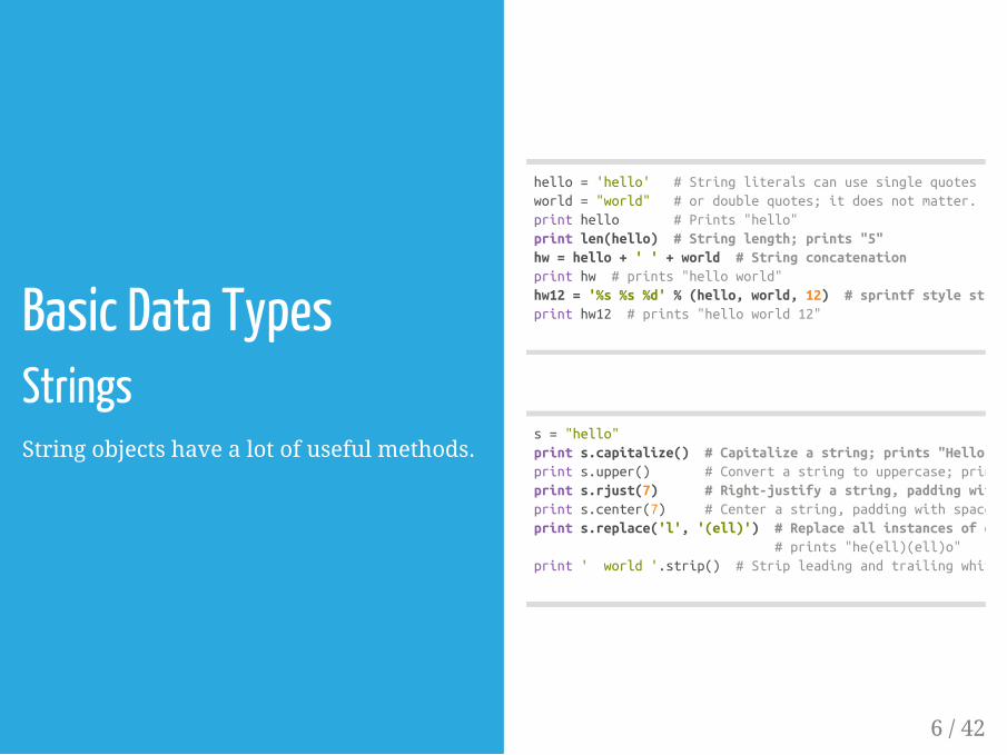
Basic Data TypesStringsString objects have a lot of useful methods.

hello = 'hello' # String literals can use single quotesworld = "world" # or double quotes; it does not matter.print hello # Prints "hello"print len(hello) # String length; prints "5"hw = hello + ' ' + world # String concatenationprint hw # prints "hello world"hw12 = '%s %s %d' % (hello, world, 12) # sprintf style string formattingprint hw12 # prints "hello world 12"

s = "hello"print s.capitalize() # Capitalize a string; prints "Hello"print s.upper() # Convert a string to uppercase; prints "HELLO"print s.rjust(7) # Right-justify a string, padding with spaces; prints " hello"print s.center(7) # Center a string, padding with spaces; prints " hello "print s.replace('l', '(ell)') # Replace all instances of one substring with another; # prints "he(ell)(ell)o"print ' world '.strip() # Strip leading and trailing whitespace; prints "world"

6 / 42

xs = [3, 1, 2] # Create a listprint xs, xs[2] # Prints "[3, 1, 2] 2"print xs[-1] # Negative indices count from the end of the list; prints "2"xs[2] = 'foo' # Lists can contain elements of different typesprint xs # Prints "[3, 1, 'foo']"xs.append('bar') # Add a new element to the end of the listprint xs # Prints x = xs.pop() # Remove and return the last element of the listprint x, xs # Prints "bar [3, 1, 'foo']"

Container TypesPython includes several built-in containertypes: lists, dictionaries, sets, and tuples.

ListsA list is the Python equivalent of an array,but is resizeable and can contain elementsof different types.

7 / 42

ContainersLists - SlicingIn addition to accessing list elements one ata time, Python provides concise syntax toaccess sublists; this is known as slicing

Lists - LoopingYou can loop over the elements of a list.

If you want access to the index of eachelement within the body of a loop, use thebuilt-in enumerate function.

nums = range(5) # range is a built-in function that creates a list of integersprint nums # Prints "[0, 1, 2, 3, 4]"print nums[2:4] # Get a slice from index 2 to 4 (exclusive); prints "[2, 3]"print nums[2:] # Get a slice from index 2 to the end; prints "[2, 3, 4]"print nums[:2] # Get a slice from the start to index 2 (exclusive); prints "[0, 1]"print nums[:] # Get a slice of the whole list; prints ["0, 1, 2, 3, 4]"print nums[:-1] # Slice indices can be negative; prints ["0, 1, 2, 3]"nums[2:4] = [8, 9] # Assign a new sublist to a sliceprint nums # Prints "[0, 1, 8, 9, 4]"

animals = ['cat', 'dog', 'monkey']for animal in animals: print animal# Prints "cat", "dog", "monkey", each on its own line.# ------animals = ['cat', 'dog', 'monkey']for idx, animal in enumerate(animals): print '#%d: %s' % (idx + 1, animal)# Prints "#1: cat", "#2: dog", "#3: monkey", each on its own line

8 / 42

nums = [0, 1, 2, 3, 4]squares = []for x in nums: squares.append(x ** 2)print squares # Prints [0, 1, 4, 9, 16]

nums = [0, 1, 2, 3, 4]squares = [x ** 2 for x in nums]print squares # Prints [0, 1, 4, 9, 16]

nums = [0, 1, 2, 3, 4]even_squares = [x ** 2 for x in nums if x % 2 == 0]print even_squares # Prints "[0, 4, 16]"

ContainersLists - List ComprehensionsWhen programming, frequently we wantto transform one type of data into another -> LC.

List comprehensions can also containconditions.

9 / 42

ContainersDictionariesA dictionary stores (key, value) pairs,similar to a Map in Java or an object inJavascript.

Dicts - LoopingIt is easy to iterate over the keys in adictionary.

If you want access to keys and theircorresponding values, use the iteritemsmethod.

d = {'cat': 'cute', 'dog': 'furry'} # Create a new dictionary with some dataprint d['cat'] # Get an entry from a dictionary; prints "cute"print 'cat' in d # Check if a dictionary has a given key; prints "True"d['fish'] = 'wet' # Set an entry in a dictionaryprint d['fish'] # Prints "wet"# print d['monkey'] # KeyError: 'monkey' not a key of dprint d.get('monkey', 'N/A') # Get an element with a default; prints "N/A"print d.get('fish', 'N/A') # Get an element with a default; prints "wet"del d['fish'] # Remove an element from a dictionaryprint d.get('fish', 'N/A') # "fish" is no longer a key; prints "N/A"

d = {'chicken': 2, 'cat': 4, 'spider': 8}for animal in d: legs = d[animal] print 'A %s has %d legs' % (animal, legs)# Prints "A chicken has 2 legs", "A spider has 8 legs", "A cat has 4 legs"

d = {'chicken': 2, 'cat': 4, 'spider': 8}for animal, legs in d.iteritems(): print 'A %s has %d legs' % (animal, legs)# Prints "A chicken has 2 legs", "A spider has 8 legs", "A cat has 4 legs"

10 / 42

nums = [0, 1, 2, 3, 4]

even_num_to_square = {x: x ** 2 for x in nums if x % 2 == 0}

print even_num_to_square # Prints "{0: 0, 2: 4, 4: 16}"

ContainersDicts - Dictionary ComprehensionsThese are similar to list comprehensions,but allow you to easily constructdictionaries.

11 / 42

ContainersSetsA set is an unordered collection of distinctelements.

animals = {'cat', 'dog'}print 'cat' in animals # Check if an element is in a set; prints "True"print 'fish' in animals # prints "False"

animals.add('fish') # Add an element to a setprint 'fish' in animals # Prints "True"

print len(animals) # Number of elements in a set; prints "3"animals.add('cat') # Adding an element that is already in the set does nothingprint len(animals) # Prints "3"

animals.remove('cat') # Remove an element from a setprint len(animals) # Prints "2"

12 / 42

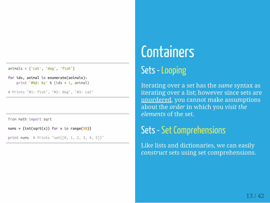
animals = {'cat', 'dog', 'fish'}

for idx, animal in enumerate(animals): print '#%d: %s' % (idx + 1, animal)

# Prints "#1: fish", "#2: dog", "#3: cat"

from math import sqrt

nums = {int(sqrt(x)) for x in range(30)}

print nums # Prints "set([0, 1, 2, 3, 4, 5])"

ContainersSets - LoopingIterating over a set has the same syntax asiterating over a list; however since sets areunordered, you cannot make assumptionsabout the order in which you visit theelements of the set.

Sets - Set ComprehensionsLike lists and dictionaries, we can easilyconstruct sets using set comprehensions.

13 / 42

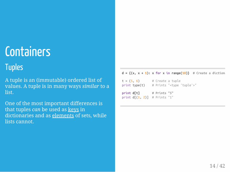
ContainersTuplesA tuple is an (immutable) ordered list ofvalues. A tuple is in many ways similar to alist.

One of the most important differences isthat tuples can be used as keys indictionaries and as elements of sets, whilelists cannot.

d = {(x, x + 1): x for x in range(10)} # Create a dictionary with tuple keys

t = (5, 6) # Create a tupleprint type(t) # Prints "<type 'tuple'>"

print d[t] # Prints "5"print d[(1, 2)] # Prints "1"

14 / 42

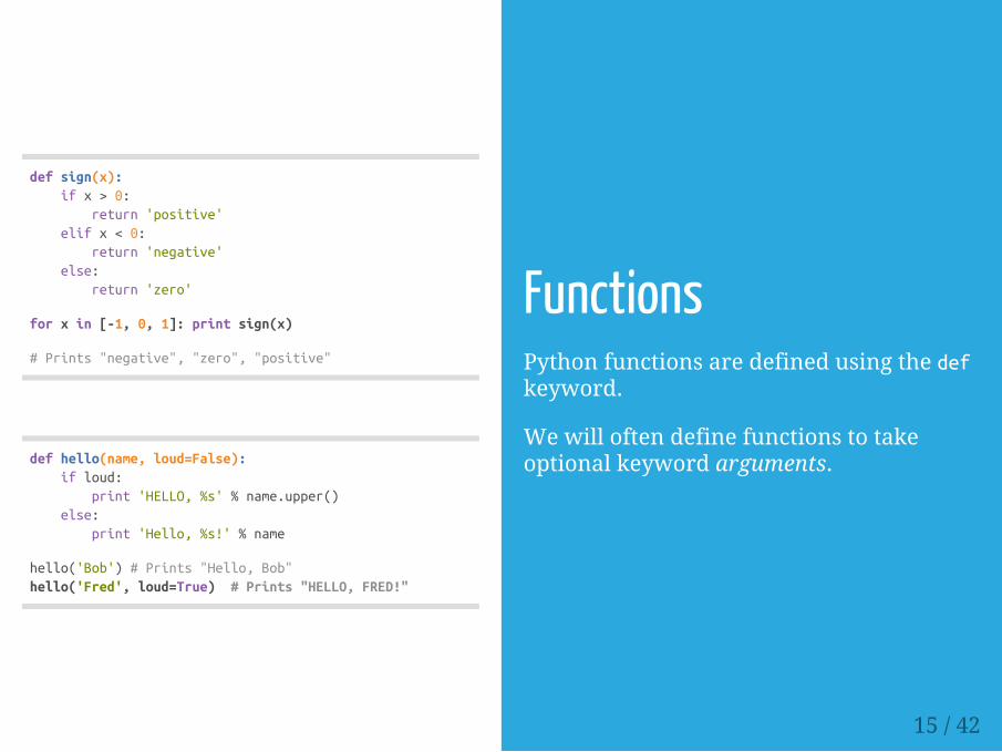
def sign(x): if x > 0: return 'positive' elif x < 0: return 'negative' else: return 'zero'

for x in [-1, 0, 1]: print sign(x)

# Prints "negative", "zero", "positive"

def hello(name, loud=False): if loud: print 'HELLO, %s' % name.upper() else: print 'Hello, %s!' % name

hello('Bob') # Prints "Hello, Bob"hello('Fred', loud=True) # Prints "HELLO, FRED!"

FunctionsPython functions are defined using the defkeyword.

We will often define functions to takeoptional keyword arguments.

15 / 42

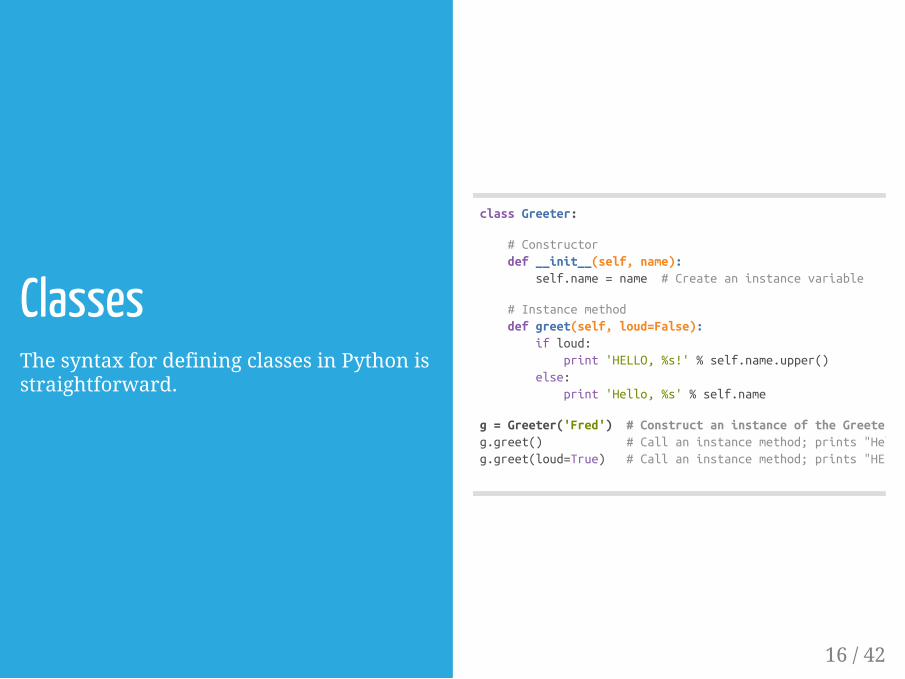
ClassesThe syntax for defining classes in Python isstraightforward.

class Greeter:

# Constructor def __init__(self, name): self.name = name # Create an instance variable

# Instance method def greet(self, loud=False): if loud: print 'HELLO, %s!' % self.name.upper() else: print 'Hello, %s' % self.name

g = Greeter('Fred') # Construct an instance of the Greeter classg.greet() # Call an instance method; prints "Hello, Fred"g.greet(loud=True) # Call an instance method; prints "HELLO, FRED!"

16 / 42

Numpy

17 / 42

Agenda1. Python Review2. Numpy

ArraysArray IndexingDatatypesArray MathBroadcasting

3. SciPy4. Matplotlib

18 / 42

import numpy as np

a = np.array([1, 2, 3]) # Create a rank 1 arrayprint type(a) # Prints "<type 'numpy.ndarray'>"print a.shape # Prints "(3,)"print a[0], a[1], a[2] # Prints "1 2 3"a[0] = 5 # Change an element of the arrayprint a # Prints "[5, 2, 3]"

b = np.array([[1,2,3],[4,5,6]]) # Create a rank 2 arrayprint b.shape # Prints "(2, 3)"print b[0, 0], b[0, 1], b[1, 0] # Prints "1 2 4"

# -----a = np.zeros((2,2)) # Create an array of all zerosprint a # Prints "[[ 0. 0.] # [ 0. 0.]]"

b = np.ones((1,2)) # Create an array of all onesprint b # Prints "[[ 1. 1.]]"

c = np.full((2,2), 7) # Create a constant arrayprint c # Prints "[[ 7. 7.] # [ 7. 7.]]"

d = np.eye(2) # Create a 2x2 identity matrixprint d # Prints "[[ 1. 0.] # [ 0. 1.]]"

e = np.random.random((2,2)) # Create an array filled with random valuesprint e # Might print "[[ 0.91940167 0.08143941] # [ 0.68744134 0.87236687]]"

NumpyNumpy is the core library for scientificcomputing in Python. It provides a high-performance multidimensional arrayobject (MATLAB style), and tools forworking with these arrays.

ArraysA numpy array is a grid of values, allof the same type, and is indexed by atuple of nonnegative integers.The number of dimensions is the rankof the array; the shape of an array is atuple of integers giving the size of thearray along each dimension.We can initialize numpy arrays fromnested Python lists, and accesselements using square brackets.Numpy also provides many functionsto create arrays.

19 / 42

NumpyArray Indexing - SlicingNumpy offers several ways to index intoarrays.

Similar to Python lists, numpy arrays canbe sliced.

Since arrays may be multidimensional, youmust specify a slice for each dimension ofthe array.

import numpy as np

# Create the following rank 2 array with shape (3, 4)# [[ 1 2 3 4]# [ 5 6 7 8]# [ 9 10 11 12]]a = np.array([[1,2,3,4], [5,6,7,8], [9,10,11,12]])

# Use slicing to pull out the subarray consisting of the first 2 rows# and columns 1 and 2; b is the following array of shape (2, 2):# [[2 3]# [6 7]]b = a[:2, 1:3]

# A slice of an array is a view into the same data, so modifying it# will modify the original array.

print a[0, 1] # Prints "2"b[0, 0] = 77 # b[0, 0] is the same piece of data as a[0, 1]print a[0, 1] # Prints "77"

20 / 42

import numpy as np

# Create the following rank 2 array with shape (3, 4)# [[ 1 2 3 4]# [ 5 6 7 8]# [ 9 10 11 12]]a = np.array([[1,2,3,4], [5,6,7,8], [9,10,11,12]])

# Two ways of accessing the data in the middle row of the array.# Mixing integer indexing with slices yields an array of lower rank,# while using only slices yields an array of the same rank as the# original array:row_r1 = a[1, :] # Rank 1 view of the second row of a row_r2 = a[1:2, :] # Rank 2 view of the second row of a

print row_r1, row_r1.shape # Prints "[5 6 7 8] (4,)"print row_r2, row_r2.shape # Prints "[[5 6 7 8]] (1, 4)"

# We can make the same distinction when accessing columns of an array:col_r1 = a[:, 1]col_r2 = a[:, 1:2]

print col_r1, col_r1.shape # Prints "[ 2 6 10] (3,)"print col_r2, col_r2.shape # Prints "[[ 2] # [ 6] # [10]] (3, 1)"

NumpyArray Indexing - SlicingYou can also mix integer indexing withslice indexing.

However, doing so will yield an array oflower rank than the original array.

Note that this is quite different from theway that MATLAB handles array slicing.

21 / 42

NumpyArray Indexing - Integer ArrayIndexingWhen you index into numpy arrays usingslicing, the resulting array view willalways be a subarray of the original array.

In contrast, integer array indexing allowsyou to construct arbitrary arrays using thedata from another array.

import numpy as np

a = np.array([[1,2], [3, 4], [5, 6]])

# An example of integer array indexing.# The returned array will have shape (3,) and print a[[0, 1, 2], [0, 1, 0]] # Prints "[1 4 5]"

# The above example of integer array indexing is equivalent to this:print np.array([a[0, 0], a[1, 1], a[2, 0]]) # Prints "[1 4 5]"

# When using integer array indexing, you can reuse the same# element from the source array:print a[[0, 0], [1, 1]] # Prints "[2 2]"

# Equivalent to the previous integer array indexing exampleprint np.array([a[0, 1], a[0, 1]]) # Prints "[2 2]"

22 / 42

import numpy as np

a = np.array([[1,2], [3, 4], [5, 6]])

bool_idx = (a > 2) # Find the elements of a that are bigger than 2; # this returns a numpy array of Booleans of the same # shape as a, where each slot of bool_idx tells # whether that element of a is > 2.

print bool_idx # Prints "[[False False] # [ True True] # [ True True]]"

# We use boolean array indexing to construct a rank 1 array# consisting of the elements of a corresponding to the True values# of bool_idxprint a[bool_idx] # Prints "[3 4 5 6]"

# ---

# We can do all of the above in a single concise statement:print a[a > 2] # Prints "[3 4 5 6]"

NumpyArray Indexing - Boolean ArrayIndexingBoolean array indexing lets you pick outarbitrary elements of an array.

Frequently this type of indexing is used toselect the elements of an array that satisfysome condition.

23 / 42

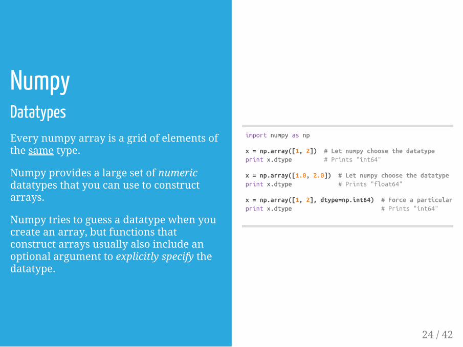
NumpyDatatypesEvery numpy array is a grid of elements ofthe same type.

Numpy provides a large set of numericdatatypes that you can use to constructarrays.

Numpy tries to guess a datatype when youcreate an array, but functions thatconstruct arrays usually also include anoptional argument to explicitly specify thedatatype.

import numpy as np

x = np.array([1, 2]) # Let numpy choose the datatypeprint x.dtype # Prints "int64"

x = np.array([1.0, 2.0]) # Let numpy choose the datatypeprint x.dtype # Prints "float64"

x = np.array([1, 2], dtype=np.int64) # Force a particular datatypeprint x.dtype # Prints "int64"

24 / 42

import numpy as np

x = np.array([[1,2],[3,4]], dtype=np.float64)y = np.array([[5,6],[7,8]], dtype=np.float64)

# Elementwise sum; both produce the array# [[ 6.0 8.0]# [10.0 12.0]]print x + yprint np.add(x, y)

# Elementwise difference; both produce the array# [[-4.0 -4.0]# [-4.0 -4.0]]print x - yprint np.subtract(x, y)

# Elementwise product; both produce the array# [[ 5.0 12.0]# [21.0 32.0]]print x * yprint np.multiply(x, y)

# Elementwise division; both produce the array# [[ 0.2 0.33333333]# [ 0.42857143 0.5 ]]print x / yprint np.divide(x, y)

# Elementwise square root; produces the array# [[ 1. 1.41421356]# [ 1.73205081 2. ]]print np.sqrt(x)

NumpyArray MathBasic mathematical functions operateelementwise on arrays, and are availableboth as operator overloads and asfunctions in the numpy module

25 / 42

NumpyArray MathNote that unlike MATLAB, * is elementwisemultiplication, not matrix multiplication.

We instead use the dot function to computeinner products of vectors, to multiply avector by a matrix, and to multiplymatrices.

dot is available both as a function in thenumpy module and as an instance methodof array objects

import numpy as np

x = np.array([[1,2],[3,4]])y = np.array([[5,6],[7,8]])

v = np.array([9,10])w = np.array([11, 12])

# Inner product of vectors; both produce 219print v.dot(w)print np.dot(v, w)

# Matrix / vector product; both produce the rank 1 array [29 67]print x.dot(v)print np.dot(x, v)

# Matrix / matrix product; both produce the rank 2 array# [[19 22]# [43 50]]print x.dot(y)print np.dot(x, y)

26 / 42

import numpy as np

x = np.array([[1,2],[3,4]])

print np.sum(x) # Compute sum of all elements; prints "10"

print np.sum(x, axis=0) # Compute sum of each column; prints "[4 6]"print np.sum(x, axis=1) # Compute sum of each row; prints "[3 7]"

import numpy as np

x = np.array([[1,2], [3,4]])print x # Prints "[[1 2] # [3 4]]"print x.T # Prints "[[1 3] # [2 4]]"

# Note that taking the transpose of a rank 1 array does nothing:v = np.array([1,2,3])

print v # Prints "[1 2 3]"print v.T # Prints "[1 2 3]"

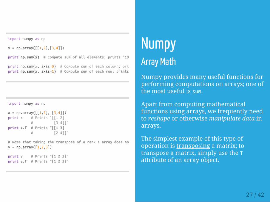
NumpyArray MathNumpy provides many useful functions forperforming computations on arrays; one ofthe most useful is sum.

Apart from computing mathematicalfunctions using arrays, we frequently needto reshape or otherwise manipulate data inarrays.

The simplest example of this type ofoperation is transposing a matrix; totranspose a matrix, simply use the Tattribute of an array object.

27 / 42

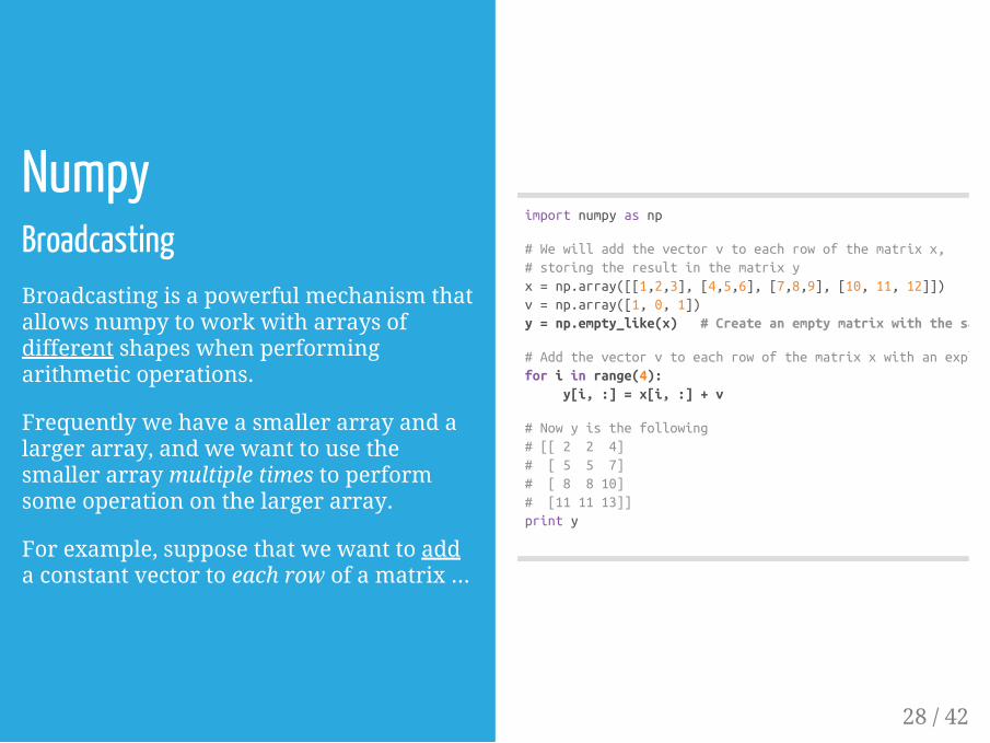
NumpyBroadcastingBroadcasting is a powerful mechanism thatallows numpy to work with arrays ofdifferent shapes when performingarithmetic operations.

Frequently we have a smaller array and alarger array, and we want to use thesmaller array multiple times to performsome operation on the larger array.

For example, suppose that we want to adda constant vector to each row of a matrix ...

import numpy as np

# We will add the vector v to each row of the matrix x,# storing the result in the matrix yx = np.array([[1,2,3], [4,5,6], [7,8,9], [10, 11, 12]])v = np.array([1, 0, 1])y = np.empty_like(x) # Create an empty matrix with the same shape as x

# Add the vector v to each row of the matrix x with an explicit loopfor i in range(4): y[i, :] = x[i, :] + v

# Now y is the following# [[ 2 2 4]# [ 5 5 7]# [ 8 8 10]# [11 11 13]]print y

28 / 42

import numpy as np

# We will add the vector v to each row of the matrix x,# storing the result in the matrix yx = np.array([[1,2,3], [4,5,6], [7,8,9], [10, 11, 12]])v = np.array([1, 0, 1])

vv = np.tile(v, (4, 1)) # Stack 4 copies of v on top of each otherprint vv # Prints "[[1 0 1] # [1 0 1] # [1 0 1] # [1 0 1]]"y = x + vv # Add x and vv elementwiseprint y # Prints "[[ 2 2 4] # [ 5 5 7] # [ 8 8 10] # [11 11 13]]"

NumpyBroadcastingThis works... however when the matrix x isvery large, computing an explicit loop inPython could be slow.

Note that adding the vector v to each rowof the matrix x is equivalent to forming amatrix vv by stacking multiple copies of vvertically, then performing elementwisesummation of x and vv.

29 / 42

NumpyBroadcastingNumpy broadcasting allows us to performthis computation without actually creatingmultiple copies of v. Consider this version,using broadcasting.

The line y = x + v works even though x hasshape (4, 3) and v has shape (3,) due tobroadcasting.

This line works as if v actually had shape(4, 3), where each row was a copy of v, andthe sum was performed elementwise.

import numpy as np

# We will add the vector v to each row of the matrix x,# storing the result in the matrix yx = np.array([[1,2,3], [4,5,6], [7,8,9], [10, 11, 12]])v = np.array([1, 0, 1])

y = x + v # Add v to each row of x using broadcastingprint y # Prints "[[ 2 2 4] # [ 5 5 7] # [ 8 8 10] # [11 11 13]]"

30 / 42

import numpy as np

# Compute outer product of vectorsv = np.array([1,2,3]) # v has shape (3,)w = np.array([4,5]) # w has shape (2,)

# To compute an outer product, we first reshape v to be a column# vector of shape (3, 1); we can then broadcast it against w to yield# an output of shape (3, 2), which is the outer product of v and w:# [[ 4 5]# [ 8 10]# [12 15]]print np.reshape(v, (3, 1)) * w

# Add a vector to each row of a matrixx = np.array([[1,2,3], [4,5,6]])# x has shape (2, 3) and v has shape (3,) so they broadcast to (2, 3),# giving the following matrix:# [[2 4 6]# [5 7 9]]print x + v# .....

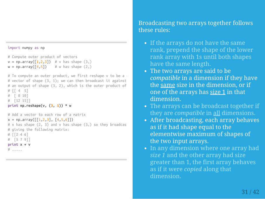
Broadcasting two arrays together followsthese rules:

If the arrays do not have the samerank, prepend the shape of the lowerrank array with 1s until both shapeshave the same length.The two arrays are said to becompatible in a dimension if they havethe same size in the dimension, or ifone of the arrays has size 1 in thatdimension.The arrays can be broadcast together ifthey are compatible in all dimensions.After broadcasting, each array behavesas if it had shape equal to theelementwise maximum of shapes ofthe two input arrays.In any dimension where one array hadsize 1 and the other array had sizegreater than 1, the first array behavesas if it were copied along thatdimension.

31 / 42

NumpyBroadcastingFunctions that support broadcasting areknown as universal functions.

Broadcasting typically makes your codemore concise and faster, so you shouldstrive to use it where possible.

# .....# Add a vector to each column of a matrix# x has shape (2, 3) and w has shape (2,).# If we transpose x then it has shape (3, 2) and can be broadcast# against w to yield a result of shape (3, 2); transposing this result# yields the final result of shape (2, 3) which is the matrix x with# the vector w added to each column. Gives the following matrix:# [[ 5 6 7]# [ 9 10 11]]print (x.T + w).T

# Another solution is to reshape w to be a row vector of shape (2, 1);# we can then broadcast it directly against x to produce the same# output.print x + np.reshape(w, (2, 1))

# Multiply a matrix by a constant:# x has shape (2, 3). Numpy treats scalars as arrays of shape ();# these can be broadcast together to shape (2, 3), producing the# following array:# [[ 2 4 6]# [ 8 10 12]]print x * 2

32 / 42

SciPy

33 / 42

Agenda1. Python Review2. Numpy3. SciPy

Image OperationsMATLAB FilesDistance between Points

4. Matplotlib

34 / 42

from scipy.misc import imread, imsave, imresize

# Read an JPEG image into a numpy arrayimg = imread('assets/cat.jpg')print img.dtype, img.shape # Prints "uint8 (400, 248, 3)"

# We can tint the image by scaling each of the color channels# by a different scalar constant. The image has shape (400, 248, 3);# we multiply it by the array [1, 0.95, 0.9] of shape (3,);# numpy broadcasting means that this leaves the red channel unchanged,# and multiplies the green and blue channels by 0.95 and 0.9# respectively.img_tinted = img * [1, 0.95, 0.9]

# Resize the tinted image to be 300 by 300 pixels.img_tinted = imresize(img_tinted, (300, 300))

# Write the tinted image back to diskimsave('assets/cat_tinted.jpg', img_tinted)

SciPyNumpy provides a high-performancemultidimensional array and basic tools tocompute with and manipulate thesearrays.

SciPy builds on this, and provides a largenumber of functions that operate on numpyarrays and are useful for different types ofscientific and engineering applications.

Image OperationsSciPy provides some basic functions towork with images.

For example, it has functions to readimages from disk into numpy arrays, towrite numpy arrays to disk as images, andto resize images.

35 / 42

SciPyMATLAB FilesThe functions scipy.io.loadmat andscipy.io.savemat allow you to read andwrite MATLAB files.

Distance between PointsSciPy defines some useful functions forcomputing distances between sets ofpoints.

The function scipy.spatial.distance.pdistcomputes the distance between all pairs ofpoints in a given set.

A similar function(scipy.spatial.distance.cdist) computesthe distance between all pairs across twosets of points.

import numpy as npfrom scipy.spatial.distance import pdist, squareform

# Create the following array where each row is a point in 2D space:# [[0 1]# [1 0]# [2 0]]x = np.array([[0, 1], [1, 0], [2, 0]])print x

# Compute the Euclidean distance between all rows of x.# d[i, j] is the Euclidean distance between x[i, :] and x[j, :],# and d is the following array:# [[ 0. 1.41421356 2.23606798]# [ 1.41421356 0. 1. ]# [ 2.23606798 1. 0. ]]d = squareform(pdist(x, 'euclidean'))print d

36 / 42

Matplotlib

37 / 42

Agenda1. Python Review2. Numpy3. SciPy4. Matplotlib

PlottingSubplotsImages

38 / 42

import numpy as npimport matplotlib.pyplot as plt

# Compute the x and y coordinates for points on a sine curvex = np.arange(0, 3 * np.pi, 0.1)y = np.sin(x)

# Plot the points using matplotlibplt.plot(x, y)plt.show() # You must call plt.show() to make graphics appear.

import numpy as npimport matplotlib.pyplot as plt

# Compute the x and y coordinates for points on sine and cosine curvesx = np.arange(0, 3 * np.pi, 0.1)y_sin = np.sin(x)y_cos = np.cos(x)

# Plot the points using matplotlibplt.plot(x, y_sin)plt.plot(x, y_cos)plt.xlabel('x axis label')plt.ylabel('y axis label')plt.title('Sine and Cosine')plt.legend(['Sine', 'Cosine'])plt.show()

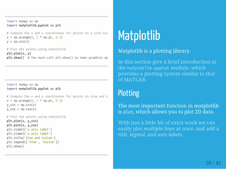
MatplotlibMatplotlib is a plotting library.

In this section give a brief introduction tothe matplotlib.pyplot module, whichprovides a plotting system similar to thatof MATLAB.

PlottingThe most important function in matplotlibis plot, which allows you to plot 2D data.

With just a little bit of extra work we caneasily plot multiple lines at once, and add atitle, legend, and axis labels.

39 / 42

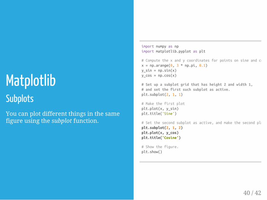
MatplotlibSubplotsYou can plot different things in the samefigure using the subplot function.

import numpy as npimport matplotlib.pyplot as plt

# Compute the x and y coordinates for points on sine and cosine curvesx = np.arange(0, 3 * np.pi, 0.1)y_sin = np.sin(x)y_cos = np.cos(x)

# Set up a subplot grid that has height 2 and width 1,# and set the first such subplot as active.plt.subplot(2, 1, 1)

# Make the first plotplt.plot(x, y_sin)plt.title('Sine')

# Set the second subplot as active, and make the second plot.plt.subplot(2, 1, 2)plt.plot(x, y_cos)plt.title('Cosine')

# Show the figure.plt.show()

40 / 42

import numpy as npfrom scipy.misc import imread, imresizeimport matplotlib.pyplot as plt

img = imread('assets/cat.jpg')img_tinted = img * [1, 0.95, 0.9]

# Show the original imageplt.subplot(1, 2, 1)plt.imshow(img)

# Show the tinted imageplt.subplot(1, 2, 2)

# A slight gotcha with imshow is that it might give strange results# if presented with data that is not uint8. To work around this, we# explicitly cast the image to uint8 before displaying it.plt.imshow(np.uint8(img_tinted))plt.show()

MatplotlibImagesYou can use the imshow function to showimages.

41 / 42

ENDEueung Mulyana

http://eueung.github.io/EL5244/py-tutbased on the material at CS231n@Stanford | Attribution-ShareAlike CC BY-SA

42 / 42