raman - nc state physics · raman induced resonance ima ging of trapped a toms b y thomas alan sa v...
TRANSCRIPT

Copyright c 1998 by Thomas Alan SavardAll rights reserved

Raman Induced Resonance Imaging of
Trapped Atoms
by
Thomas Alan Savard
Department of PhysicsDuke University
Date:Approved:
Dr. John E. Thomas, Supervisor
Dr. Berndt M�uller
Dr. Bob D. Guenther
Dr. Daniel J. Gauthier
Dr. Joshua E. S. Socolar
Dissertation submitted in partial ful�llment of therequirements for the degree of Doctor of Philosophy
in the Department of Physicsin the Graduate School of
Duke University
1998

abstract
(Physics)
Raman Induced Resonance Imaging of
Trapped Atoms
by
Thomas Alan Savard
Department of PhysicsDuke University
Date:Approved:
Dr. John E. Thomas, Supervisor
Dr. Berndt M�uller
Dr. Bob D. Guenther
Dr. Daniel J. Gauthier
Dr. Joshua E. S. Socolar
An abstract of a dissertation submitted in partial ful�llment ofthe requirements for the degree of Doctor of Philosophy
in the Department of Physicsin the Graduate School of
Duke University
1998

Abstract
This dissertation describes the development of the �rst neutral atom trap-
ping apparatus at Duke University and Raman induced resonance imaging of
trapped atoms|an imaging technique which provides three-dimensional in-
formation about the atomic spatial distribution in the trap. The design and
operating principles of the 6Li atom source, laser sources, multi-coil Zeeman
slower, and magneto-optic trap used in the experiment are explained. Using
Raman induced resonance imaging, the atomic spatial distribution in the
magneto-optic trap is imaged with 12�m resolution. Changes to the exper-
iment will yield a resolution of 5�m|rivaling the best resolution achieved
in previous two-dimensional imaging experiments|without the expense of
large aperture optics and high resolution cameras.
The position distribution of atoms is acquired by inducing Raman transi-
tions between lithium's ground state hyper�ne levels. The quadrupole mag-
netic �eld of the MOT causes the Raman transition strength and Raman
resonance frequency to vary with position. By measuring the response of
the atomic distribution at di�erent Raman pulse frequencies, a spectrum is
obtained which depends on the position distribution of the atoms.
iv

ABSTRACT v
Previous images of trapped atoms used CCD cameras to record uores-
cence or phase contrast images of the atomic spatial distribution. Because the
CCD camera measures only two-dimensional information, the entire depth
of the trap was averaged onto a single plane. In Raman induced resonance
imaging of the MOT, the number of atoms in concentric ellipsoidal shells
is measured. Consequently, Raman induced resonance imaging is ideally
suited for probing small centrally located density variations within high den-
sity atomic spatial distributions, a regime in which two-dimensional imaging
with a camera is unsuitable.
In this dissertation, Raman induced resonance imaging is used to deter-
mine the size of the atomic distribution and it's o�set relative to the MOT's
magnetic �eld zero point. The center of the atomic cloud is found to be sub-
stantially shifted from the magnetic �eld zero point of the trap. In addition,
the work presented here signi�cantly advances the development of single-
shot Raman transient imaging techniques that will have wide applications to
fundamental measurements of ultracold trapped atoms.

Acknowledgments
I would �rst like to thank John Thomas for all his guidance and enthusiasm
in the completion of this work. John was always there with a thoughtful
word of encouragement or a brilliant insight whenever I needed it. I have
learned quantum mechanics, machining, mathematics, plumbing, and even
some motivational psychology from John|all of which I hope to make use
of in the future.
I also must thank Jack Netland, my high school physics teacher, who �rst
introduced me to physics. The fun and enthusiasm he brought to the science
classroom had a signi�cant impact on my decision to study physics.
Dean Langley, my advisor at St. John's University, sparked my interest
in optics and gave me my �rst signi�cant research opportunity. Thank you
for giving me the opportunity and fostering my desire to explore.
While at Duke I have had the privilege to work with many wonderful
people. I would like to thank all those who graduated from my group before
me: Pat, Kevin, Je�, Allan, Carl, Mike, and Zhao. They showed me most
of what I know in the lab and didn't give me too hard of a time when I did
things wrong. I would especially like to thank Carl Schnurr who has been a
vi

ACKNOWLEDGMENTS vii
great friend (and sometimes counselor) over the years.
If it weren't for all the help I've had in recent years from Ken O'Hara,
Mike Gehm, and especially Stephen Granade, this project would never have
been completed. Ken worked with me in the early days and end days of
the experiment and built the diode laser and MOT magnet controller (the
Hummer) used in the experiment. Mike assisted in a variety of ways, ei-
ther in by assembling parts of the Hummer, staying late with me to run the
experiment, or drawing up some the �gures for this dissertation. For most
of the last year, Stephen assisted me daily in running the experiment (even
on Christmas Eve!) or by machining some brackets for who knows what.
Stephen also got the camera system working and wrote the computer pro-
grams for the data analysis. I also want to thank Chris Baird who helped
me build the slower. I couldn't have had a better crew helping me with this
experiment!
Adam Wax and Zehuang Lu, although not directly involved with my ex-
periment, provided invaluable assistance in times of need. Adam's expertise
in heterodyne detection was frequently called upon during the some of the
initial experiments and he was always willing to lend a helping hand or optic.
During my desperate attempts to �x our ailing dye laser in December, Lu
gave us his own dye pump when ours went bad (yes, Coherent, they do go
bad!) Their sel essness during the diÆcult months of the experiment is very
much appreciated.
I would also like to thank the Samir Bali who provided insight into dif-

ACKNOWLEDGMENTS viii
ferent aspects of the experiment, especially toward its conclusion.
Richard Poole, now retired, showed me, with great patience, how to safely
use the instruments in the machine shop. With his guidance, I gained the
skills to create the apparatus for my experiment. I'm sorry new students
won't get to learn from him. I hope he enjoys his retirement free from the
distractions of ying bits and chuck keys!
Thanks also to my friends back home|Mike, Scott, and Darin| and
my friends and classmates at Duke. Thanks especially to Mike Bergmann,
fellow Minnesotan, Johnnie, and Dukie, who helps keep alive the memories
of comfortable summers and unbearable winters back in Minnesota.
My parents and family all deserve thanks for keeping me optimistic and
encouraging me to pursue my dreams. That's two dreams accomplished,
now, and many more to go!
Most importantly, I wish to thank my wife, Lynda, for all her love and
support through graduate school. Her patience, faith, and music kept me
sane, especially during the last few months. I look forward to spending more
time with her and becoming the president of her fan club!

For Lynda, with love
ix

Contents
Abstract iv
Acknowledgments vi
List of Figures xiv
List of Tables xviii
1 Introduction 1
1.1 Motivation for the Current Work . . . . . . . . . . . . . . . . 3
1.2 Raman Induced Resonance Imaging . . . . . . . . . . . . . . . 10
1.2.1 Description of Raman Induced ResonanceImaging . . . . . . . . . . . . . . . . . . . . . . . . . . 10
1.2.2 Spatial Resolution . . . . . . . . . . . . . . . . . . . . 13
Spectral Resolution . . . . . . . . . . . . . . . . . . . . 13
Velocity-Limited Resolution . . . . . . . . . . . . . . . 15
Acceleration-Limited Resolution . . . . . . . . . . . . . 16
1.2.3 The Spatial Resolution Function . . . . . . . . . . . . . 17
1.3 Overview of the Current Work . . . . . . . . . . . . . . . . . . 18
x

CONTENTS xi
1.4 Organization of the Dissertation . . . . . . . . . . . . . . . . . 22
2 Raman Transitions in Magnetic Fields 23
2.1 Raman Transitions in a Three level Atom . . . . . . . . . . . . 25
2.1.1 The Three-Level Amplitude Equations . . . . . . . . . 26
2.1.2 Reduction to a Two-Level System . . . . . . . . . . . . 28
2.1.3 The Final State Probability . . . . . . . . . . . . . . . 31
2.2 Raman Transitions of 6Li Atoms in a Magnetic Field . . . . . 34
2.2.1 Multiple Two-Level Systems . . . . . . . . . . . . . . . 34
2.2.2 Magnetic Field Dependence of the Raman Spectrum . 38
2.2.3 Raman Spectrum of 6Li in a Magnetic Field . . . . . . 45
3 Properties of Lithium 47
3.1 Physical Properties . . . . . . . . . . . . . . . . . . . . . . . . 48
3.2 Thermodynamic Properties . . . . . . . . . . . . . . . . . . . 49
3.3 Electromagnetic Properties . . . . . . . . . . . . . . . . . . . . 52
3.3.1 Energy Level Structure . . . . . . . . . . . . . . . . . . 52
3.3.2 Optical Transition Strength . . . . . . . . . . . . . . . 54
3.3.3 Optical Rabi Frequency . . . . . . . . . . . . . . . . . 54
3.3.4 Dipole Moment Matrix Elements . . . . . . . . . . . . 56
3.3.5 Raman Rabi Frequencies . . . . . . . . . . . . . . . . . 59
3.3.6 The E�ect of Magnetic Fields on the Raman Transitions 64
4 Cooling and Trapping Apparatus 68

CONTENTS xii
4.1 The Oven . . . . . . . . . . . . . . . . . . . . . . . . . . . . . 69
4.2 The Vacuum System . . . . . . . . . . . . . . . . . . . . . . . 75
4.2.1 Vacuum System Components . . . . . . . . . . . . . . 75
4.2.2 Vacuum System Procedures . . . . . . . . . . . . . . . 79
Daily Operation . . . . . . . . . . . . . . . . . . . . . . 80
Startup Procedures and Bakeout . . . . . . . . . . . . 81
Shutdown Procedure . . . . . . . . . . . . . . . . . . . 84
4.3 The Lasers . . . . . . . . . . . . . . . . . . . . . . . . . . . . . 85
4.4 Multi-Coil Zeeman Slower . . . . . . . . . . . . . . . . . . . . 88
4.4.1 Background . . . . . . . . . . . . . . . . . . . . . . . . 88
4.4.2 Magnet Design . . . . . . . . . . . . . . . . . . . . . . 97
4.4.3 Slower Current Supplies . . . . . . . . . . . . . . . . . 102
4.4.4 Coil Con�guration . . . . . . . . . . . . . . . . . . . . 107
4.4.5 The atom's trajectory . . . . . . . . . . . . . . . . . . 109
4.4.6 Required Optical Fields . . . . . . . . . . . . . . . . . 113
4.4.7 Observation of Slow Atoms . . . . . . . . . . . . . . . 115
4.5 Magneto-Optic Trap . . . . . . . . . . . . . . . . . . . . . . . 118
4.5.1 Background and Required Optical Fields . . . . . . . . 119
4.5.2 The Magnets . . . . . . . . . . . . . . . . . . . . . . . 122
4.5.3 Optical Detection of the MOT . . . . . . . . . . . . . . 130
5 The Imaging Experiment 134
5.1 Optical Layout . . . . . . . . . . . . . . . . . . . . . . . . . . 136

CONTENTS xiii
5.2 Pulse Timing and Data Acquisition . . . . . . . . . . . . . . . 146
5.3 Experimental Procedures . . . . . . . . . . . . . . . . . . . . . 152
6 Results 161
6.1 Analysis of the Central Lineshape and the Resolution . . . . . 164
6.2 Calculating a Theoretical Spectrum . . . . . . . . . . . . . . . 168
6.3 The Measured Raman Spectra . . . . . . . . . . . . . . . . . . 182
7 Conclusion 197
7.1 Summary . . . . . . . . . . . . . . . . . . . . . . . . . . . . . 198
7.2 Future of Raman Imaging in Traps . . . . . . . . . . . . . . . 200
A The Transition Dipole Moments 206
Bibliography 209
Biography 217

List of Figures
1.1 The atomic distribution is sampled in shells of constant mag-netic �eld strength. . . . . . . . . . . . . . . . . . . . . . . . . 8
1.2 Schematic of Raman induced resonance imaging. . . . . . . . . 11
1.3 Energy level diagram of the Raman transition. . . . . . . . . . 12
2.1 Non-resonant Raman transitions in a three-level atom. . . . . 26
2.2 Possible Raman transitions within the J = 1=2 ground stateof 6Li in the presence of a magnetic �eld. . . . . . . . . . . . . 35
2.3 Tuning of the Raman transitions in a magnetic �eld. . . . . . 39
2.4 The e�ect of the magnetic �eld on the quantization axis in theatom's frame. . . . . . . . . . . . . . . . . . . . . . . . . . . . 41
3.1 Steady state number of trapped atoms for alkalis in a vaporcell MOT. . . . . . . . . . . . . . . . . . . . . . . . . . . . . . 51
3.2 Energy level diagram of 6Li. . . . . . . . . . . . . . . . . . . . 53
3.3 Transition dipole moments of the D2 line in6Li. . . . . . . . . 57
3.4 Transition dipole moments of the D1 line in6Li. . . . . . . . . 58
3.5 Energy level diagram of a 6Li Raman transition. . . . . . . . . 60
3.6 6Li Raman transitions in a magnetic �eld. . . . . . . . . . . . 66
4.1 A schematic of the apparatus used to cool and trap the atoms. 68
xiv

LIST OF FIGURES xv
4.2 The oven. . . . . . . . . . . . . . . . . . . . . . . . . . . . . . 71
4.3 Schematic diagram of the vacuum system. . . . . . . . . . . . 76
4.4 The trapping region. . . . . . . . . . . . . . . . . . . . . . . . 78
4.5 Photons absorbed and spontaneously emitted by an atom. . . 89
4.6 The number of atoms leaving the oven with speed v and di-rection (�; �). . . . . . . . . . . . . . . . . . . . . . . . . . . . 94
4.7 An atom's trajectory before, during, and after deceleration inrelation to the trapping volume. . . . . . . . . . . . . . . . . . 95
4.8 Coil geometry and wire wrapping eÆciency. . . . . . . . . . . 98
4.9 The multi-coil Zeeman slower. . . . . . . . . . . . . . . . . . . 101
4.10 A diagram of the slower current supply. . . . . . . . . . . . . . 103
4.11 The circuit mask for the slower current supply. . . . . . . . . . 104
4.12 The circuit mask for the slower main board. . . . . . . . . . . 106
4.13 Magnetic �eld pro�les of the slower coils. . . . . . . . . . . . . 107
4.14 Desired and measured magnetic �eld pro�les. . . . . . . . . . . 108
4.15 Slower �eld used in imaging experiment. . . . . . . . . . . . . 110
4.16 Atomic trajectories in the slower. . . . . . . . . . . . . . . . . 111
4.17 Rate of atoms entering and leaving the slower as a function ofvelocity. . . . . . . . . . . . . . . . . . . . . . . . . . . . . . . 112
4.18 Velocity distributions with a weak slowing beam. . . . . . . . 113
4.19 Schematic for measuring the rate of atoms entering the trap-ping region at a speci�c velocity. . . . . . . . . . . . . . . . . . 116
4.20 Fluorescence signal from a slowed atomic beam. . . . . . . . . 117
4.21 Atoms slowed to trapping velocities. . . . . . . . . . . . . . . . 118

LIST OF FIGURES xvi
4.22 The schematic diagram for a magneto-optic trap. . . . . . . . 119
4.23 A one-dimensional energy diagram for an atom in a MOT. . . 120
4.24 The positions of the MOT magnets. . . . . . . . . . . . . . . . 124
4.25 The schematic diagram for a MOT magnet current supply. . . 125
4.26 The circuit board layout for the MOT current supply. . . . . . 126
4.27 The circuit board layout for the MOT magnet main controllerboard. . . . . . . . . . . . . . . . . . . . . . . . . . . . . . . . 127
4.28 The uorescence of the MOT captured by a CCD camera. . . 132
4.29 The absorption of the MOT captured by a CCD camera. . . . 133
5.1 A schematic of the four steps used to generate a point in theRaman spectrum. . . . . . . . . . . . . . . . . . . . . . . . . 135
5.2 The layout of the modulators for creating the MOT beams. . . 139
5.3 Schematic of the MOT beam optical elements. . . . . . . . . 140
5.4 The Raman imaging experiment showing MOT beams and theadditional Raman and pump/probe beams. . . . . . . . . . . . 142
5.5 The optical layout for the imaging experiment. . . . . . . . . . 145
5.6 The timing of the pulses during the imaging experiment. . . . 146
5.7 The experimentally measured time dependence of the uores-cence caused by a single series of imaging pulses. . . . . . . . . 150
5.8 The steps followed in measuring a Raman spectrum. . . . . . . 153
5.9 The experimentally measured uorescence spectrum of 6Li. . . 154
6.1 A typical Raman spectrum shows �ve peaks. . . . . . . . . . . 163
6.2 The magnetic independent resonance determines the spectralresolution. . . . . . . . . . . . . . . . . . . . . . . . . . . . . . 165

LIST OF FIGURES xvii
6.3 The fractional power variation in the tunable Raman �eld. . . 178
6.4 Calculated spectra for di�erent spatial distributions. . . . . . . 181
6.5 Two di�erent Raman spectra taken with di�erent trap laserbeam detunings. . . . . . . . . . . . . . . . . . . . . . . . . . . 183
6.6 Additional Raman spectra taken with di�erent trap laser beamdetunings. . . . . . . . . . . . . . . . . . . . . . . . . . . . . . 184
6.7 Fluorescence images of the trap taken with di�erent trap laserbeam detunings. . . . . . . . . . . . . . . . . . . . . . . . . . . 185
6.8 Fits of the di�erent Raman spectra when the Raman pulsearea is a �tting parameter. . . . . . . . . . . . . . . . . . . . . 187
6.9 Additional �ts of Raman spectra when the Raman pulse areais a �tting parameter. . . . . . . . . . . . . . . . . . . . . . . . 188
6.10 The 1/e trap size along the major axes as a function of traplaser beam detuning. . . . . . . . . . . . . . . . . . . . . . . . 189
6.11 The o�set of the trap with respect to the magnetic �eld zero. . 190
6.12 The 1/e constant density surface of the MOT. . . . . . . . . . 193
6.13 The density in the x� y plane at z = 600 �m. . . . . . . . . . 194
6.14 The density in the y � z plane at x = 0 �m. . . . . . . . . . . 195
6.15 The density in the x� z plane at y = 0 �m. . . . . . . . . . . 196
7.1 The energy level diagram for Raman transient imaging. . . . . 202
7.2 A schematic for optical heterodyne detection. . . . . . . . . . 203
7.3 The free-induction decay signal from atoms loaded into theMOT. . . . . . . . . . . . . . . . . . . . . . . . . . . . . . . . 204

List of Tables
3.1 Raman Rabi frequency magnitudes. . . . . . . . . . . . . . . . 64
3.2 Raman resonance frequency shifts in a magnetic �eld. . . . . . 67
4.1 Nozzle temperature gradient. . . . . . . . . . . . . . . . . . . . 73
4.2 The free spectral range (FSR) of the tuning elements in thedye laser. . . . . . . . . . . . . . . . . . . . . . . . . . . . . . 86
4.3 Slower coil currents used in verifying the �tting procedure. . . 108
4.4 Slower coil currents used in the imaging experiment. . . . . . . 110
4.5 Physical parameters for the MOT coils. . . . . . . . . . . . . . 122
4.6 The MOT coil currents used during the imaging experiment. . 123
5.1 The laser beams required in the imaging experiment. . . . . . 137
5.2 Typical MOT beam powers. . . . . . . . . . . . . . . . . . . . 141
6.1 The �tting parameters used in the calculated spectra. . . . . . 180
xviii

Chapter 1
Introduction
In 1997, the Royal Swedish Academy of Sciences awarded the Nobel Prize in
Physics to William Phillips, Stephen Chu, and Claude Cohen-Tannoudji for
the development of techniques to optically cool and trap atoms. Even though
their accomplishments are relatively recent|the �rst three-dimensional cool-
ing was reported by Chu et al. in 1985 [1]|their pioneering research in opti-
cal forces [1{15] has already led to a profound impact in atomic physics and
beyond.
For example, the realization of Bose condensates in trapped atoms has
provided low temperature physics with a novel quantum degenerate uid [16{
22] and led to the creation of the �rst atom laser [23]. Optical tweezers, which
are based on the light forces used to cool and trap atoms, are routinely used
in the biological sciences to manipulate intracellular objects being examined
under microscope. In addition, optical lattices, which con�ne atoms in the
periodic potentials created by optical standing waves, demonstrate long range
order and may improve our understanding of more complex systems in solid
1

CHAPTER 1. INTRODUCTION 2
state physics [24{27]. Moreover, in nuclear physics, the measurement of par-
ity nonconserving transition rates in trapped francium isotopes will explore
the electroweak interaction [28,29]. Because trapped atoms provide high den-
sity samples, small inhomogeneous broadening, and long interaction times to
the researcher, they are an excellent medium for the study of fundamental
interactions.
Regardless of the context in which trapped atoms are being studied, one
of the most important properties to measure is the atoms' position distribu-
tion. For a practical application, consider atoms trapped in a conservative
potential. The atoms' position distribution determines the mean energy and
temperature of the atoms. In another application, at low enough tempera-
tures, the position distribution provides an interesting means of exploring the
quantum statistics of fermions and bosons [30{36]. Thus, the position dis-
tribution can be a simple diagnostic or a highly physical means of observing
some of the deepest features of quantum mechanics.
This dissertation describes Raman induced resonance imaging of trapped
atoms|a technique which provides three-dimensional information about the
sample of trapped atoms. A combination of laser beams and magnetic �elds
is used to create a magneto-optic trap (MOT) [9]. The magnetic �eld used
to create the trap is, in turn, used to create spatially dependent Raman
transition strengths and resonance frequencies. When the trapped atoms are
probed with a laser beam that induces Raman transitions, the response of
the sample depends on the atomic spatial distribution. During the imag-

CHAPTER 1. INTRODUCTION 3
ing experiment described herein, this response is measured and is used to
describe the atomic spatial distribution with 12�m resolution. Changes to
the experiment will yield a resolution of 5�m|rivaling the best resolution
achieved in previous two-dimensional imaging experiments|without the ex-
pense of large aperture optics and high resolution cameras. Raman induced
resonance imaging is ideally suited for probing small centrally located den-
sity variations within high density atomic spatial distributions, a regime in
which two-dimensional imaging with a camera is unsuitable. Moreover, since
Raman induced resonance imaging measures the atomic spatial distribution
with respect to the magnetic �eld zero of the trap, the technique should prove
useful in experiments which are sensitive to magnetic �elds.
1.1 Motivation for the Current Work
Currently, the spatial distributions of trapped atoms are measured with
charge-coupled device (CCD) cameras. In traps which make use of the spon-
taneous photon scattering force, the atoms emit a considerable amount of
uorescence which provides a simple mechanism for measuring the spatial
distribution. The uorescence is imaged onto a CCD camera which gen-
erates a two dimensional plot of intensity. For low atomic densities, the
intensity measurement of each pixel represents the density of atoms inte-
grated along the pixel's line of sight. Density measurements of this type
have been performed in a number of experiments [37{43]. However, under

CHAPTER 1. INTRODUCTION 4
certain circumstances, these techniques possess a number of disadvantages.
First, at densities of 1011 atoms=cc such as those acquired in magneto-
optic traps (MOT) [9, 13, 37, 39, 41, 43, 44] the distribution in the MOT can
become optically thick and signi�cantly attenuate the lasers that provide the
trapping force. Under these conditions, the uorescence of the atoms in the
center of the distribution will be less intense than that of the atoms at the
edge. As a result, the atoms in the center of the trap will not contribute
equally to the line of site density measured by the pixel. When the densi-
ties become so high that the MOT is noticeably optically thick, the most
interesting spatial distributions develop [37, 41, 43].
Townsend et al. review the three density regimes attainable in standard
MOTs [41]. At low densities, the MOT behaves like an ideal gas con�ned
in a harmonic potential with two di�erent spring constants. As such, the
MOT possesses a Gaussian density distribution. The two spring constants
are due to the quadrupole magnetic �eld that is used to create a MOT. Along
one axis of the MOT, the quadrupole magnetic �eld creates a magnetic �eld
gradient that is twice as steep as it is along the other two axes. Using the
equipartition theorem, the nominal radius r of the atomic distribution along
a particular axis is predicted and measured [37, 39, 41] to go as
r =
rkBT
�(1.1)
where kB is the Boltzmann constant, T is the temperature of the distribution,

CHAPTER 1. INTRODUCTION 5
and � is the spring constant. Thus, in this regime, the trap should have an
ellipsoidal shape with the minor and major axes related byp2. In this
regime, the size of the cloud remains the same regardless of the number
of trapped atoms. This low density behavior has been observed by two
groups [37, 41].
The low densities described above rarely occur in a typical MOT. Under
most circumstances, the density in the MOT is high enough that interac-
tions between the atoms diminish the ideal gas behavior. The interactions
are caused by radiation trapping forces [37] which occur when photons are
scattered from multiple atoms in the trap. Because the scattered photons
from one atom exert radiation pressure on nearby atoms, the atomic density
cannot increase inde�nitely. As more and more atoms are added to the trap,
the trap size increases with an approximately uniform maximum density.
Rather than having a Gaussian spatial distribution, the distribution has a
at pro�le and is approximately spherical. Sesko et al. [37] used uorescent
imaging to measure this type of distribution, but Townsend et al. [41] noted
that the atomic distribution is well approximated by a Gaussian unless small
magnetic gradients are applied and trap laser frequency detunings are small.
At low trap detunings, however, the condition that photons scatter multi-
ple times in the medium is equivalent to the atoms possessing a minimum
amount of optical thickness. Consequently, CCD uorescence measurements
in this regime with small trap detunings may be unreliable.
The third regime for MOT spatial distributions occurs at high densities,

CHAPTER 1. INTRODUCTION 6
large magnetic �eld gradients and large trap frequency detunings. Using
numerical analysis, two groups [45, 46] predicted that a two component dis-
tribution will exist in the MOT in this regime. A spatially narrow and dense
distribution which arises from strong polarization gradient [14] forces should
exist in the low magnetic �eld region at the center of the trap, surrounded by
a large distribution with a much lower density. Two-dimensional uorescence
measurements by Townsend et al. [41] and Petrich et al. [43] indicated the
two-component behavior of the distributions at large detunings and magnetic
�eld gradients.
The size of the central distribution along an axis of the MOT is deter-
mined by the frequency dependence of the polarization gradient force which
peaks sharply as a function of detuning. In the presence of the magnetic
�eld of the MOT, the Zeeman shift of the cooling transitions determines the
detuning at a particular point in space. Thus, at some small distance from
the trap center, there is a sharp peak in the con�ning force of the MOT. If
the polarization gradient force peaks at a detuning of �p, the radius of the
narrow distribution in that direction will be given by
�BdBi
dxixi = �h�p (1.2)
where �B is the Bohr magneton, dBi=dxi is the magnetic �eld gradient along
the i axis, and xi is the displacement. In this regime, since the gradient along
one axis of the MOT is twice as high as along the others, the minor and major

CHAPTER 1. INTRODUCTION 7
axes of the atomic distribution are related by a factor of two. Townsend et
al. observed the appropriate scaling between the axes of the central feature
in a MOT over a limited set of data. This regime is characterized by high
densities and optical thickness which Townsend et al. cited as a limit in their
theory and measurement methods.
The problems of optical thickness in uorescence measurements may be
somewhat alleviated by the phase contrast techniques [47] implemented in
imaging optically thick Bose condensates [19, 48, 49]. However, this method
still uses a CCD camera which integrates the depth of the atomic distribution
onto a single plane of information. Small centrally located features may be
indistinguishable when averaged in this way.
Helmerson et al. [50] performed the only known previous imaging exper-
iment in which the atomic distribution was not measured using line of sight
averaging and a CCD camera. They used laser spectroscopy to measure a
one-dimensional distribution of atoms in a superconducting magnetic trap.
The atoms in the large 25 cm long trap had Zeeman shifts which varied over
600MHz. By measuring the absorption of a weak probe laser as a function
of frequency, the spatial distribution of the atoms was measured. In this
technique, the doppler shift limits the resolution to approximately 3:5mm.
While this method provided adequate resolution for the large trap in their
experiment, the resolution is clearly inadequate for most traps in use today
which have diameters less than their resolution.
Raman induced resonance imaging possesses high resolution and over-

CHAPTER 1. INTRODUCTION 8
Cloud of atomsin the MOT
Shell of constant|B|
r0
Figure 1.1: The atomic distribution is sampled in shells of constant mag-netic �eld strength. The center of the atomic distribution may be o�set fromthe center of the shells.
comes both the limitations imposed by optically thick samples and line of
sight averaging. Resonance imaging is performed with a series of pulses and
only a small fraction of the atoms interact with a given pulse. Thus, the
e�ective depth of the atoms is considerably reduced so that optical thick-
ness becomes negligible. In addition, the shape of the atomic distributions
that are sampled by each pulse need not be planar. Rather, the sampling
shape may be implemented to more accurately match the symmetry of the
distribution being measured.
In this dissertation, an optically thick sample of atoms in a magneto-
optic trap is imaged using Raman induced resonance imaging. Because the
quadrupole magnet �eld of the MOT is used for the imaging, the atoms
are sampled in ellipsoidal shells, as shown in Figure 1.1. This new method
of imaging trapped atoms allows one to measure spatial distributions that

CHAPTER 1. INTRODUCTION 9
are inaccessible to uorescence measurements and inconvenient to measure
using line of sight methods. In addition, the atomic spatial distribution is
measured with respect to the magnetic �eld zero of the trap thereby providing
important information for experiments which are sensitive to magnetic �elds.
The resolution of the technique demonstrated here is 12�m which is
equivalent to the best resolution [41] obtained in the uorescence measure-
ments. Changes to the experiment described in this dissertation should yield
resolutions of 5�m which is limited by the motion of atoms in the trap.
With colder atoms, the resolution reaches a limit of 510 �A which can only
be improved by increasing the magnetic �eld gradient in the MOT. In con-
trast, the best resolution obtained using the phase contrast imaging tech-
niques [19, 48, 49] is 4� 5�m which is near the practical resolution limit
imposed on aperture-limited classical optical techniques.
The resonance imaging technique presented in this dissertation can be
directly applied to other traps with quadrupole magnetic �elds. In particular,
a new high-�eld-gradient quadrupole magnetic trap developed by Vuletic
et al. adiabatically compresses the atoms in a MOT into a ball less than
200�m in diameter [51]. Because of the extremely large magnetic �elds used
in this trap, absorptive and uorescence measurements with a CCD camera
are not feasible. In the 3�105G=cm gradient of their trap, the resonance
imaging would have a resolution of 157 nm immediately after the atoms are
adiabatically compressed into the trap. For cooled atoms in their trap, the
Raman induced resonance imaging resolution approaches 30 nm. Moreover,

CHAPTER 1. INTRODUCTION 10
the spatial extent of the wavefunction for atoms con�ned in the ground state
of their trap is much less than an optical wavelength. Consequently, if most of
the atoms are cooled to the ground state, spatial imaging will require the sub-
optical resolution attainable by the techniques developed in this dissertation.
1.2 Raman Induced Resonance Imaging
Previous experiments by our group demonstrated Raman Induced Resonance
Imaging (RIRI) in a number of atomic beam experiments [52{54]. Three
theoretical papers [36, 55, 56] as well as two review papers [34, 35] have been
published on RIRI as well.
1.2.1 Description of Raman Induced Resonance
Imaging
To understand how RIRI works, it is worthwhile to review standard resonance
imaging techniques. In resonance imaging, an atomic spatial distribution is
initially in one initial state jii, as shown in Figure 1.2. The energy of another
state, called the �nal state jfi is shifted using a force �eld. For example, in
the �gure, the �nal state is shifted by a magnetic �eld gradient. This causes
the transition frequency between jii and jfi, !0(x), to vary in space. If an
excitation pulse of frequency ! with the appropriate intensity and duration
interacts with the atoms, the atoms located at the place where ! = !0(x)
can be placed into the �nal state. In the �gure, this location is denoted by

CHAPTER 1. INTRODUCTION 11
f
i
AtomicDistributionω ω0(x)
x0
∆x
Magnetic FieldGradient
B(x)
Figure 1.2: Schematic of Raman induced resonance imaging.
x0. The number of atoms in the �nal state is detected after the excitation
pulse. The number of atoms detected corresponds to the number of atoms in
the initial state at x0 before the pulse. If the atomic distribution is recreated
in the initial state, and the excitation pulse is repeated with a di�erent !, a
di�erent set of atoms will be detected in the �nal state corresponding to a
di�erent resonant location x0.
By repeatedly measuring the sample at di�erent excitation frequencies,
the number of atoms that originated in the initial state can be expressed
as a function of excitation frequency. Since the resonant location is a well-
de�ned function of excitation frequency, x0(!; !0), the spatial distribution
of the atoms can be determined. As shown in Figure 1.2, the resolution
of the imaging technique is given by �x which is simply the width of the
distribution that is excited at a particular x0. The resolution is discussed in

CHAPTER 1. INTRODUCTION 12
I
i
f
∆
ω2ω1
ωω0(x)
Figure 1.3: Energy level diagram of the Raman transition.
Section 1.2.2.
Raman induced resonance imaging operates with the same principles. Es-
sentially, the only di�erence between Raman and standard resonance imaging
is the method used to create the excitation pulse. As shown in Figure 1.3,
the excitation pulse is created by combining two optical �elds of frequency !1
and !2. The di�erence in the frequency of the two �elds, called the Raman
di�erence frequency, acts as the excitation frequency ! of the pulse. In the
�gure, the di�erence frequency is given by ! = !1 � !2. The Raman transi-
tion, a two-photon process, proceeds through state jIi which is o�-resonant
with !1 and !2 by the detuning �.
Like most forms of resonance imaging, Raman induced resonance imaging
uses a series of Raman pulses with di�erent ! to map out a spatial distribu-
tion. We \scan" the Raman transition frequency ! in order to measure the
spatial distribution. Scanning is straightforward in an atomic beam because
the spatial distribution in the beam remains essentially constant in the lab
frame. Perturbations applied to the distribution as a result of the measure-

CHAPTER 1. INTRODUCTION 13
ment process are carried downstream. New atoms continually repopulate the
interesting spatial distribution.
Raman induced resonance imaging may be used in a MOT because the
MOT possesses a large trap depth and can also be rapidly recycled. In the
lithium MOT, the trap depth is at least 0:5K. Although the atoms absorb
photons during the measurement process, the perturbation is on the order of
a few microkelvin, and is negligible compared to the depth of the trap. Con-
sequently, the MOT recycles nearly instantaneously, in a few microseconds.
1.2.2 Spatial Resolution
Three factors limit the spatial resolution of RIRI: spectral resolution, motion
of atoms during the Raman transition, and di�raction of the atoms due to
localization. I will present heuristic derivations for each of these limits in
this section. The precise results depend on the speci�cs of the particular
experiment.
Spectral Resolution
The spectral resolution of the Raman transition is one of the three factors
limiting the spatial resolution, �x, of RIRI. The e�ective linewidth of the
Raman transition and the bandwidth of the Raman �elds determine the
spectral resolution. Because we choose long-lived ground states for jii andjfi, the transition is free from traditional radiative broadening. However, if
the detuning from the excited state, �, is too small, thus allowing incoherent

CHAPTER 1. INTRODUCTION 14
transitions from the ground states to the excited states, this long lifetime
reduces to the incoherent transition time. Usually, we make the detuning
large enough to prevent signi�cant population of the excited state. In this
limit, the bandwidth of the Raman transition is negligible.
We reduce the bandwidth of the Raman �elds using three techniques.
First, because the Raman �elds copropagate, the Doppler shift due to the
atomic motion cancels in !, the Raman di�erence frequency. Secondly, we
use the same light source and nominal path lengths for both Raman �elds
so that frequency jitter from the laser source cancels in the Raman di�er-
ence frequency. Finally, to create the di�erence frequency, we use standard
stable acousto-optic modulators which have a typical stability of 1 kHz in
100MHz [57]. Because the di�erence frequency is so stable, the duration
T of the Raman pulse usually determines the spectral resolution �! as a
consequence of Fourier's theorem. Thus,
�! � 1=T (1.3)
The spatial resolution due to the spectral resolution can be determined
by noting that when the energy shift of jfi varies linearly with position, as
shown in Figure 1.2, the energy gradient exerts a uniform force F on jfi.Thus, the spatial tuning rate of the Raman resonance frequency is given by
the quantity F=h which has units of Hz/cm. It describes how quickly the
Raman transition resonance frequency changes as a function of position along

CHAPTER 1. INTRODUCTION 15
the measurement axis. By noting that
�! =F
�h�x; (1.4)
the spatial resolution for a pulse of length T can be written as
�x = �xsp =�h
FT: (1.5)
Velocity-Limited Resolution
Atomic motion during the Raman pulses also a�ects the spatial resolution. If
the atoms have a velocity vx along the measurement axis during the Raman
pulse, they will move a distance vxT during the the measurement. Atoms
which were initially out of the resonant region may move into the resonant
region during this time. Consequently, the minimum velocity limited resolu-
tion �xvel is given by �xvel = vxT . In this limit, lower velocities and shorter
measurement times produce better resolution. However, (1.5) shows that T
cannot be made arbitrarily short because the spectral resolution limit will
eventually dominate the spatial resolution. By setting �xvel = �xsp, one can
solve for the ideal measurement time Tvel to determine the actual velocity
limited resolution.
Tvel =
��h
vxF
�1=2
: (1.6a)

CHAPTER 1. INTRODUCTION 16
Using (1.6a) in the expression for �xvel gives
�xvel =
�vx�h
F
�1=2
: (1.6b)
Acceleration-Limited Resolution
The third limiting factor in the spatial resolution occurs due to di�raction.
The di�raction limit is caused by the acceleration of the atoms due to F
during the measurement process. By localizing the atoms, we necessarily
perturb them with a force. During the measurement time T the atom moves
a distance due to acceleration given by FT 2=2m, where m is the mass of
the atom. Again, the shorter we make T the better, until the spectroscopic
resolution is reached. Following the same analysis used in the velocity limit,
Tacc =
�2�hm
F 2
�1=3
(1.7a)
�xacc =
��h2
2mF
�1=3
: (1.7b)
The most fundamental limit to the spatial resolution is the acceleration
limit. For a given spatial tuning rate, the acceleration limit is determined
for a particular atom. The velocity limited resolution also depends on the
spatial tuning rate but may be improved using an atomic beam with better
collimation or by additional cooling of atoms in a trap.
In the acceleration limit, Raman Induced Resonance Imaging can, under

CHAPTER 1. INTRODUCTION 17
certain circumstances, be uncertainty-principle limited. To see this, consider
the case when the spatially varying potential only shifts one state in the
transition; in this case, assume only jfi is shifted. Consequently, the force
F will act only on the atom after it is has made the transition from jii tojfi. Because the atom can make the transition to jfi anytime during the
duration, T , of the measurement, there is a net uncertainty in the atom's
momentum after the measurement, given by �p = FT . If the resolution is
given by the spectroscopic limit which has been set equal to the velocity-
and di�raction-limited resolutions in (1.6) and (1.7), the uncertainty in the
position is given by �x = �h=FT . Thus, the uncertainty product is
�p�x � FT�h
FT= �h: (1.8)
For Gaussian Raman pulses, the full quantum mechanical calculation in
Ref. [55] shows that (1.8) reduces to �p�x = �h=2 in the ideal case.
1.2.3 The Spatial Resolution Function
For Raman Induced Resonance Imaging, the probability for the atom to be
in the �nal state Pf after the Raman pulse takes a general form. If x is the
measurement axis, this probability is given by [52, 53, 56]
Pf(!) =
Zdpx
ZdxR(!; x; px)Wi(x; px) (1.9)

CHAPTER 1. INTRODUCTION 18
where ! is the Raman di�erence frequency, Wi(x; px) is the phase space
distribution of the atoms in the initial state, and R(!; x; px) is the resolution
function. For each !, there is some x = x0 where the resolution function
peaks sharply. The frequency distribution of the Raman pulses and the
shape of the potential gradient determines the exact shape of R(!; x; px).
Since the resolution of the technique may be limited by either the velocity
of the atoms or the acceleration of the atoms during the measurement, the
momentum of the atoms is necessarily included in R and the complete phase
space density Wi(x; px) is needed.
Experimentally, we measure the the �nal state population as a function
of the Raman di�erence frequency. Through careful characterization of the
gradient potential, we can relate the Raman di�erence frequency to the spa-
tial measurement axis. Since the �nal state population is proportional to
the probability Pf(!), the measurements of the �nal state represent this
probability as ! is scanned through the possible resonance frequencies.
Given the potential gradient, we can calculate the resolution function,
R(!; x; px). With this resolution function, we can �nd Wi(x; px) with a reso-
lution determined by R(!; x; px) by �tting the calculated Pf(Æ) to the data.
1.3 Overview of the Current Work
In the current work, Raman Induced Resonance Imaging (RIRI) is used to
measure the spatial distribution of lithium atoms in magneto-optic trap.

CHAPTER 1. INTRODUCTION 19
The atoms originate in an atomic beam with a most probable velocity of
1680m=s. The atoms with velocities below 1100m=s are decelerated using
counterpropagating radiation to a �nal velocity near 40m=s. The slow atoms
propagate into a magneto-optic trap (MOT) which binds and cools them to
approximately 350�K and an average velocity of 1m=s. When the number
of trapped atoms reaches an equilibrium, the atomic distribution is measured
using resonance imaging in the quadrupole magnetic �eld provided by the
MOT.
While imaging the atoms, the laser beams used in the MOT are momen-
tarily turned o�. After the atoms are placed into the initial imaging state,
the jF = 1=2i ground state, a Raman pulse with a particular di�erence fre-
quency induces Raman transitions to the �nal state, the jF = 3=2i groundstate. Due the magnetic �eld dependence of the Raman transitions, described
in Chapter 2, only atoms in the region with the appropriate magnetic �eld
strength make the transition to the �nal state.
The quadrupole magnetic �eld of the MOT creates ellipsoidal shells of
constant �eld strength in position space as shown in Figure 1.1. Imbalances
between the laser beams used to make the (MOT) frequently cause the atomic
cloud to be o�set from the magnetic �eld zero of the MOT as shown. The
thickness of each shell corresponds to the resolution, �x. After the atoms
in the shell are placed in the �nal state, they are detected using resonance
uorescence. Immediately after the uorescence of the �nal state is recorded,
the MOT trapping beams are turned back on to recycle the trap and the

CHAPTER 1. INTRODUCTION 20
MOT quickly returns to it's original shape. This measurement process is
repeated for di�erent Raman di�erence frequencies, thereby measuring the
uorescence corresponding to the number of atoms in each ellipsoidal shell
in the MOT.
The spectrum of the �nal state uorescence as function of Raman dif-
ference frequency is compared to a calculated expression for the spectrum.
This calculated expression is in the form of the �nal state probability (1.9)
de�ned in Section 1.2.3. The resolution function de�ned by (1.9) is derived
for an arbitrary magnetic �eld in Chapter 2 and determined speci�cally for
the quadrupole �eld of the MOT in Chapter 6. Based on the operating pa-
rameters of the magneto-optic trap, the expected form of the atomic density
function is used to calculate the theoretical spectrum. Then, this calculated
spectrum is �t to the experimentally measured Raman spectrum to obtain
spatial information about the atomic cloud. The sensitivity of the Raman
spectrum to the atomic spatial distribution allows the size and o�set of the
trapped atom cloud to be determined. The o�set of the cloud is measured
relative to the magnetic �eld zero of the trap.
Our group was required to learn and apply a signi�cant amount of tech-
nology to accomplish this experiment. These technologies included:
ultra-high vacuum (UHV) systems A UHV system with ultimate pres-
sures near 5�10�11 torr provides long trap decay times for this and
future experiments.

CHAPTER 1. INTRODUCTION 21
a non-standard laser dye Since the cooling transition in lithium occurs
at 671 nm, an initially troublesome, yet eventually worthwhile, non-
standard dye is required to achieve signi�cant power (over 700mW) at
this wavelength.
a multi-coil Zeeman slower A Zeeman slower permitted deceleration of
a lithium beam for loading into a magneto-optic trap. The slower
decelerates atoms from 1100m=s to 40m=s.
a magneto-optic trap (MOT) The MOT, the workhorse of almost every
trapping experiment, captures � 108 atoms and cools them to a few
hundred microkelvin and average velocities of 1m=s.
The work presented here represents an excellent technique for imaging
traps which can be recycled quickly like the MOT. Since the technique may
be applied to optically thick atomic distributions, Raman induced resonance
imaging o�ers a method of probing dense traps for which traditional uo-
rescence trap imaging is unsuitable. In addition, resonance imaging allows
one to measure the atomic distribution by sampling with a resolution func-
tion that matches the trap symmetry. Since this avoids averaging the image
across the depth of the trap, Raman induced resonance imaging is particu-
larly useful in exploring small density variations at the center of the atomic
distribution.

CHAPTER 1. INTRODUCTION 22
1.4 Organization of the Dissertation
This dissertation is comprised of seven chapters and one appendix. In Chap-
ter 2, the �nal state probability (1.9) is calculated for a distribution of 6Li
atoms in an arbitrary magnetic �eld. This is the �rst calculation of a resolu-
tion function that includes multiple Raman transitions and the prospect of
three-dimensional imaging. Chapter 3 explains why we chose lithium, specif-
ically 6Li, to use in the experiment. Then, the relevant thermodynamic and
electromagnetic properties of lithium and their implications are discussed.
In Chapter 4, the cooling and trapping apparatus is described. The chap-
ter details the vacuum system, laser systems, multi-coil Zeeman slower, and
magneto-optic trap used in the experiment. The apparatus and procedures
used in the imaging phase of the experiment are described in Chapter 5. The
results of the imaging experiment are presented and analyzed in Chapter 6.
There, the general expression for the �nal state probability derived in Chap-
ter 2 is applied to the speci�c quadrupole �eld of the MOT. An expression
for the atomic density distribution is found by �tting the calculated spectra
to the data. In Chapter 7, the results of the dissertation are summarized
and future applications of Raman induced imaging are discussed. Finally,
Appendix A details how the transition dipole moment matrix elements pre-
sented in Chapter 3 were calculated.

Chapter 2
Raman Transitions in Magnetic
Fields
In the experiment described in Chapter 5, Raman induced resonance imag-
ing is used to measure the spatial distribution of atoms in a magneto-optic
trap (MOT). The quadrupole magnetic �eld of the MOT, described in Sec-
tion 4.5.2, creates spatially varying Zeeman shifts which correlate the Raman
transition frequency of a particular atom with it's location in the magnetic
�eld. Before the measurement, all of the atoms are in one internal state,
denoted the initial state. Then, a Raman pulse induces transitions in some
atoms from the initial state to a �nal state. The Raman pulse contains two
optical frequencies, the di�erence of which is called the Raman di�erence
frequency. Only those atoms with a Raman transition frequency near the
Raman di�erence frequency make the transition to the �nal state. After the
Raman pulse, the number of atoms in the �nal state is detected using res-
onance uorescence. This process is repeated for several Raman di�erence
frequencies, creating a Raman spectrum.
23

CHAPTER 2. RAMAN TRANSITIONS IN MAGNETIC FIELDS 24
The Raman spectrum contains information about the atomic spatial dis-
tribution. The number of atoms in the �nal state at each Raman di�erence
frequency is proportional to the probability that an atom made the transi-
tion. The general form for this probability is
Pf(!) =
Zdpx
ZdxR(!; x; px)Wi(x; px) (2.1)
as described in Section 1.2.3. The speci�c expression depends on the mag-
netic �eld strength and direction, the bandwidth of the Raman pulse, and
the spatial distribution of the atoms. In this chapter, an explicit expression
for the �nal state probability is derived. As a function of Raman di�erence
frequency, this probability is the Raman spectrum measured in the experi-
ment.
This theory chapter consists of two sections. In the �rst section, the semi-
classical amplitude equations for a Raman transition are derived. I treat
the center of mass motion of the atom classically because the experiment is
operated in the spectral resolution limit in which the bandwidth of the Raman
pulse and the Raman transition linewidth determine the resolution. Thus,
the atom's motion during the Raman pulse has a negligible e�ect on its �nal
state probability. At the end of the �rst section, an approximate expression
for the three-level atom Raman spectrum is obtained. The second section of
this chapter extends the probability derived in the �rst section to account
for the nonuniform magnetic �eld of the MOT and the spatial distribution

CHAPTER 2. RAMAN TRANSITIONS IN MAGNETIC FIELDS 25
of the atoms. The result is Raman spectrum in the form of (2.1).
2.1 Raman Transitions in a Three level Atom
Figure 2.1 depicts the energy levels and optical frequencies involved in the
Raman transition. The atom is initially in state jii. The Raman pulse
contains two optical �elds with frequencies !1 and !2 and couples jii to jfithrough the intermediate state jIi. As shown, the optical �elds are detunedfrom resonance with jIi by �1 and �2, respectively, which are approximately
equal. The initial and �nal state internal energies are given by �h!i and �h!f ,
respectively. The notation !nm implies !n � !m. Thus,
!fi = !f � !i (2.2)
!12 = !1 � !2: (2.3)
Using this picture, an approximate solution for the atom's �nal state proba-
bility is calculated. The resulting probability, expressed as a function of the
optical �eld strengths and the Raman detuning, Æ = !12�!fi, can be viewedas an expression of a three-level atom Raman spectrum.
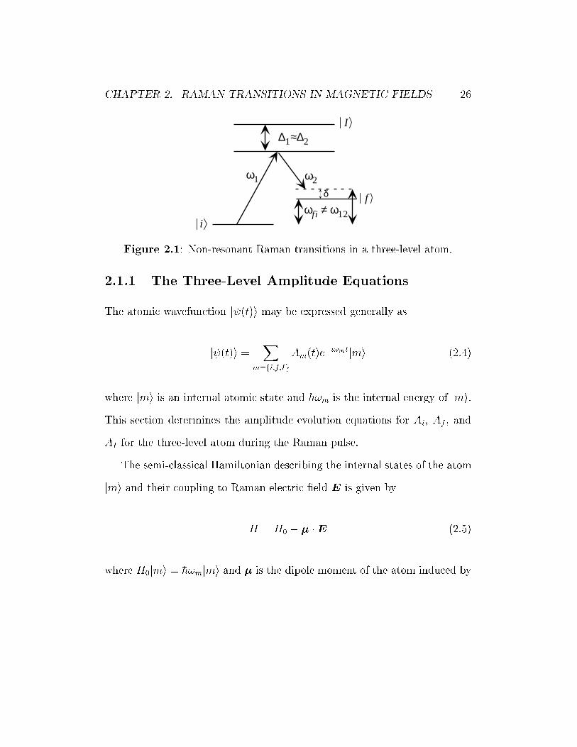
CHAPTER 2. RAMAN TRANSITIONS IN MAGNETIC FIELDS 26
I
i
f
∆1≈∆2
ω2ω1
δ
ωfi ≠ ω12
Figure 2.1: Non-resonant Raman transitions in a three-level atom.
2.1.1 The Three-Level Amplitude Equations
The atomic wavefunction j (t)i may be expressed generally as
j (t)i =X
m=fi;f;Ig
Am(t)e�i!mtjmi (2.4)
where jmi is an internal atomic state and �h!m is the internal energy of jmi.This section determines the amplitude evolution equations for Ai, Af , and
AI for the three-level atom during the Raman pulse.
The semi-classical Hamiltonian describing the internal states of the atom
jmi and their coupling to Raman electric �eld E is given by
H = H0 � � �E (2.5)
where H0jmi = �h!mjmi and � is the dipole moment of the atom induced by

CHAPTER 2. RAMAN TRANSITIONS IN MAGNETIC FIELDS 27
E. The electric �eld is described by
E =E1
2e�i!1t + c:c: +
E2
2e�i!2t + c:c: (2.6)
Due to a combination of selection rules and detuning, jii and jfi are onlycoupled to jIi via E1 and E2, respectively.
The wavefunction for the internal state of the atom must evolve according
to the Schr�odinger equation:
Hj (t)i = i�h@
@tj (t)i: (2.7)
By projecting the state hnj onto (2.7) and making the rotating wave ap-
proximation, we get the following equations of motion for the amplitudes:
_Ai(t) = ��1
2iAI(t)e
i�1t (2.8a)
_Af (t) = ��2
2iAI(t)e
i�2t (2.8b)
_AI(t) = �1
2iAi(t)e
�i�1t � 2
2iAf (t)e
�i�2t � �
2AI(t): (2.8c)
Here, �1 = !1 � !Ii and �2 = !2 � !If . Also in (2.8) are the optical Rabi
frequencies 1 = �Ii �E1=�h and 2 = �If �E2=�h. The �=2 term was added
heuristically in (2.8c) to provide a linewidth for the optical transitions and
to allow the population in the intermediate (excited) state to decay.

CHAPTER 2. RAMAN TRANSITIONS IN MAGNETIC FIELDS 28
2.1.2 Reduction to a Two-Level System
To reduce the three amplitude equations to two, we �rst assume a solution
to (2.8c) of the form AI(t) = a1(t)e�i�1t + a2(t)e
�i�2t. Inserting this into
(2.8c) and separating the di�erent frequency components gives
_a1(t) + a1(t)
��
2� i�1
�= �1
2iAi(t) (2.9a)
_a2(t) + a2(t)
��
2� i�2
�= �2
2iAf (t) (2.9b)
We assume that �1;�2 � n;�. Since a1 and a2 vary at rates on the order
of n, the optical Rabi frequencies, �1a1 � _a1 and �2a2 � _a2. Thus, we
may neglect the boxed terms to obtain an approximate expression for AI(t).
This approximate solution is
AI(t) � �Ai(t)1
2i��2� i�1
�e�i�1t � Af(t)2
2i��2� i�2
�e�i�2t: (2.10)
Inserting this approximate solution for AI(t) into (2.8a) and (2.8b) gives
_Ai(t) =�j1j2�2 + 4�2
1
��
2+ i�1
�Ai(t)� �
12
�2 + 4�22
��
2+ i�1
�Af (t)e
�i(�2��1)t
(2.11a)
_Af (t) =�j2j2�2 + 4�2
2
��
2+ i�2
�Af(t)� �
21
�2 + 4�21
��
2+ i�2
�Ai(t)e
�i(�1��2)t:
(2.11b)

CHAPTER 2. RAMAN TRANSITIONS IN MAGNETIC FIELDS 29
The �=2 terms in (2.11) describe spontaneous transitions from o� resonant
excitation of jIi. Because we have assumed that �1;�2 � �, we will neglect
these terms in the calculation of the Raman spectrum.
The light shift �m [58] and Raman Rabi frequency � are de�ned as
�m =jmj2�m
�2 + 4�2m
(2.12)
� = �2�12�2
�2 + 4�22
: (2.13)
In the limit where �1 � �2 � �� � these reduce to
�m =jmj24�
(2.14)
� = ��12
2�: (2.15)
Using (2.14) and (2.15), we can rewrite (2.11) as
_Ai(t) = �i�1Ai(t) +i�
2Af(t)e
iÆt (2.16a)
_Af(t) = �i�2Af(t) +i��
2Ai(t)e
�iÆt (2.16b)
where �1 ��2 = !12 � !fi � Æ, the Raman detuning.
The light shift terms in (2.16) simply cause a change in the Raman res-
onance frequency, as seen by replacing Ai(t) with ai(t)e�i�1t and Af(t) with
af(t)e�i�2t. After we perform this substitution, the amplitude equations be-

CHAPTER 2. RAMAN TRANSITIONS IN MAGNETIC FIELDS 30
come
_ai(t) =i�
2af (t)e
i(� �2��1 )t (2.17a)
_af (t) =i��
2ai(t)e
�i(� �2��1 )t: (2.17b)
For imaging experiments, the two light shifts be made equal everywhere in
the sample, making the boxed terms zero. This is accomplished by using an
intensity ratio for the optical �elds in the Raman pulse such that �1 = �2.
Without balanced light shifts in the sample, the �nite size of the Raman
pulse beam would lead to an unwanted spatial dependence in the Raman
transition frequency, in addition to the desired spatial dependency provided
by the applied potential.
Now that the intermediate state jIi has been adiabatically eliminated,
the Raman transition can be viewed in a two-level atom picture. Neglecting
the boxed terms in (2.17), the Hamiltonian which describes the two level
system is given by
H = H0 ���h�
2e�i!12tjiihf j+H:C:
�(2.18)
where H0 is still the internal atomic Hamiltonian as de�ned in (2.5). In
this expression for the two-level Hamiltonian, we see the Raman transition
operator. In Section 2.2, we consider rotations to this operator due to a ro-
tating quantization axis. The varying magnetic �eld direction in the MOT's

CHAPTER 2. RAMAN TRANSITIONS IN MAGNETIC FIELDS 31
quadrupole �eld leads to this rotation.
2.1.3 The Final State Probability
With (2.17), we may solve for the �nal state probability after the Raman
pulse, jAf(t ! 1)j2. First, we will solve the resonant Æ = 0 case to de-
termine how the �nal state probability depends on the Rabi frequency and
pulse duration. Then, using �rst order perturbation theory, we will solve the
non-resonant case to determine how the �nal state probability depends on
the detuning Æ. A combination of the two results provides an approximate
solution for the �nal state probability that simpli�es the numerical analysis.
If we set Æ = 0 in (2.17), the equations reduce to a simple set of di�erential
equations. Taking the time derivative of (2.17) with Æ = 0, we get
�ai(t) = i�
2a0f(t) (2.19a)
�af(t) = i��
2a0i(t): (2.19b)
Combining (2.17) and (2.19), the di�erential equation for the �nal state
amplitude becomes
�af(t) +j�j24af(t) = 0: (2.20)
With the initial condition that af (t) = 0, the solution is af (t) = sin(j�jt=2).For a square Raman pulse of length � in the interval (�1 < t < 1), the

CHAPTER 2. RAMAN TRANSITIONS IN MAGNETIC FIELDS 32
�nal state probability is given by
Pf(t!1) = jAf(t!1)j2 = sin2j�j�2: (2.21)
The quantity j�j� is known as the pulse area and quanti�es the coherent
transitions from jii to jfi. A pulse area of �=2 transfers half the population
of jii to jfi while a � pulse transfers all of it. For Raman Induced Resonance
Imaging, a � pulse is usually used to transfer all of the atoms to jfi at theresonant location.
The nonresonant solution may be solved exactly, but to simplify the anal-
ysis, we use perturbation theory and assume that ai(t) � 1. Then, (2.17b)
may be integrated. For a square Raman pulse of length � (centered at t = 0
for convenience), the solution is:
af(t!1) =
Z �=2
��=2
dt0i��t0
2e�iÆt
0
=i��
Æsin
�
2: (2.22)
so that
Pf(t!1) =� 2j�j24
sinc2�
2(2.23)
where
sinc x =sin x
x: (2.24)

CHAPTER 2. RAMAN TRANSITIONS IN MAGNETIC FIELDS 33
As one would expect, the nonresonant solution evaluated at Æ = 0 approx-
imately equals the resonant solution when j�j� � 1. Thus, for small pulse
areas, we may view (2.23) as the product of (2.21) with a sinc lineshape func-
tion that depends on the detuning Æ. However, Marable and Welch [59, 60]
found that for pulse areas as large as 4�, the lineshape remains approxi-
mately constant. Therefore, we will combine the resonant and nonresonant
solutions to form an approximate general solution given by
Pf(Æ) = sin2j�j�2
sinc2�
2(2.25)
Only the magnitude of the Raman Rabi frequency determines the value
of the �nal state probability. Rather than continuing to write the magnitude
notation, henceforth j�j will be replaced by � to denote the Rabi frequency
magnitude.
As a function of the Raman detuning, Æ, the �nal state probability in
(2.25) represents a Raman spectrum. We now have an approximate solution
for the �nal state probability as a function of pulse area and detuning. In the
next section, we will modify (2.25) for multilevel atoms in a spatially varying
magnetic �eld.

CHAPTER 2. RAMAN TRANSITIONS IN MAGNETIC FIELDS 34
2.2 Raman Transitions of 6Li Atoms in a
Magnetic Field
So far we have only considered the Raman transition in a simple three-level
atom. To image the atoms, perpendicular linearly polarized Raman �elds
are used to induce Raman transitions within 6Li's J = 1=2 ground state in
the quadrupole magnetic �eld of the MOT. In this section, I modify the �nal
state probability (2.25) to account for the multiple levels in lithium and the
presence of the magnetic �eld.
2.2.1 Multiple Two-Level Systems
The two levels in the 6Li ground state, as shown in Figure 2.2, are split by
228MHz. Each F -level contains 2F + 1 degenerate mF -levels. Thus, the
initial state jii contains two levels and the �nal state jfi contains four levels.The presence of a magnetic �eld removes the degeneracy of the mF levels
through the Zeeman shift as shown. The arrows denote the possible Raman
transitions from jii to jfi.The intermediate state jIi is the excited state J 0 = 3=2 level which con-
tains three F 0-levels. In this section, we will consider only how the multiple
initial and �nal states a�ect the �nal state probability. The e�ect of the
multiple intermediate states is treated in Section 3.3 where the Raman Rabi
frequencies and light shifts are calculated.
In general, the selection rule �m = 0;�1;�2 governs a Raman transition

CHAPTER 2. RAMAN TRANSITIONS IN MAGNETIC FIELDS 35
{ 228 MHzmF = -3/2 3/2-1/2
F = 3/2
F = 1/2
1/2
i
f
J = 1/2
J’ = 3/2 I 1/2
F’ = 3/25/2
{
Figure 2.2: Possible Raman transitions within the J = 1=2 ground state of6Li in the presence of a magnetic �eld.
since it is a two photon process where one photon is absorbed and one is
emitted. To understand why �m = �2 transitions are not allowed in 6Li (as
well as other J = 1=2 ground state atoms), we can consider the two-photon
process in terms of tensor operators. The combination of two one-photon
processes creates three possible tensor operators. The overall interaction is
a product of atom operators and �elds that yields either a scalar, vector, or
outer product operator. The scalar operator which is proportional to to E1 �E�
2is identically zero in this case since the polarizations of the electric �elds
are perpendicular. However, the rank-one vector operator is proportional to
E1�E�
2and is nonzero, leading to the Raman transitions shown in Figure 2.2.
In addition, a rank-two operator may also be formed which is proportional
to the outer product E1 E�
2. However, because the Raman transition
occurs within the J = 1=2 ground state, the rank two Raman transition is

CHAPTER 2. RAMAN TRANSITIONS IN MAGNETIC FIELDS 36
not allowed. The Raman Rabi frequency, as calculated in Section 3.3, for
the �m = �2 transitions is identically zero. This occurs because no vector
combination of 1/2 and 2 results in 1/2. Consequently, only �m = 0;�1transitions occur in the J = 1=2 ground state.
In the experiment, Raman transitions from jii = jF = 1=2i to jfi =jF = 3=2i are induced. As shown in the Figure 2.2, in the presence of the
magnetic �eld, these transitions occur at di�erent frequencies. If the mag-
netic �eld splits the Raman transition by more than the Raman transition
linewidth, only one transition is resonant for each atom at any particular Ra-
man di�erence frequency. In this limit, we may treat each Raman transition
as a separate two-level atom process.
In deriving (2.25), we made a number of assumptions about the two-
level process, most notably that the boxed light shift terms in (2.17) cancel
over the sample. In the multi-level picture shown in Figure 2.2, the Raman
�elds couple two initial states to four �nal states. To assure that the �nal
state probability only depends on the atom's position in the magnetic �eld,
the light shifts for each level must be equal. Since the experiment uses
linearly polarized optical �elds in the Raman pulse, this is remarkably easy
to accomplish.
The light shift of 6Li's ground states in the presence of linearly polarized
light is a scalar quantity and is independent of m. We can understand why
this occurs by exploring the physical mechanism of the light shift. The ex-
pressions for the light shift (2.14) and Raman Rabi frequency (2.15) show

CHAPTER 2. RAMAN TRANSITIONS IN MAGNETIC FIELDS 37
the similarity of the two processes. Whereas a Raman transition uses stimu-
lated absorption from one electric �eld and stimulated emission into another
�eld to couple two di�erent states, the light shift describes the e�ect of stimu-
lated absorption and emission from the same �eld on one state. Both Raman
transitions and the light shift occur as a result of two-photon processes.
If we consider the light shift in the tensor operator viewpoint, the scalar
behavior of the light shift is easily understood. As explained when we consid-
ered the rank-two Raman tensor operator, the rank-two light shift operator
cannot operate in the J = 1=2 basis. Since the light shift results from a two-
photon process from the same linearly polarized electric �eld, the rank-one
operator proportional to Em�E�
m is identically zero. Thus, only the scalar
operator formed from the dot product produces the light shift. Consequently,
the light shift is independent of mF . Thus, the light shifts of all the �nal
states are identical and the light shifts of all the initial states are identical.
To create equal light shifts for all of the �nal and initial states, the ratio
of the intensities of E1 and E2 are adjusted as described in Sections 2.1.2
and 3.3.
Since the light shifts of each state in every possible Raman transition can-
cel, the two-level probability (2.25) describes each transition independently
as long as the magnetic �eld is large enough to resolve each transition. For
an individual atom, this corresponds to the condition the Raman transitions
are separated in frequency more than the linewidth of the Raman transitions.
Since the magnitude of the MOT's quadrupole �eld continually increases over

CHAPTER 2. RAMAN TRANSITIONS IN MAGNETIC FIELDS 38
the range of the atomic distribution from a central magnetic �eld zero point,
the multiple two-level approximation holds as long as the atom is suÆciently
removed from the magnetic �eld zero.
In our experiments, atoms more than 18�m from the magnetic center
may be treated by this approximation. Note that the magnetic �eld center
does not necessarily correspond to the center of atomic distribution. Since
the radius of the atomic distribution is approximately 350�m, the fraction
of atoms that may not be treated in this approximation goes as (18=350)3
which is less than one percent. Consequently, the contribution these atoms
make to the �nal state population may be neglected in the calculation of the
Raman spectrum.
2.2.2 Magnetic Field Dependence of the Raman
Spectrum
The previous section explained why each of the Raman transitions shown in
Figure 2.2 may be treated independently. Before the measurement, the ini-
tial state is prepared by equally populating both jF = 1=2; mF = �1=2i andjF = 1=2; mF = 1=2i. Depending on the atom's position in the quadrupole
magnetic �eld, it may make any one of the Raman transitions shown in
Figure 2.2. Each transition has a separate Raman Rabi frequency and de-
tuning which depend on the atom's position in the magnetic �eld. Thus, the

CHAPTER 2. RAMAN TRANSITIONS IN MAGNETIC FIELDS 39
{ mF =
F = 3/2
F = 1/2i
f
J = 1/2 228 MHz3/2-1/2 1/2
10-1∆m =
γm,1/2 = 0 2/3 4/3
Figure 2.3: Tuning of the Raman transitions in a magnetic �eld.
probability expressed in (2.25) may be rewritten as
Pf(t!1; Æ) =1
2
Xi
sin2(�i(r)�
2) sinc2(
(Æ � ÆBi (r))�
2) (2.26)
where i is summed over each of the transitions. The factor of one-half occurs
because the atom may be in either initial state. The Raman Rabi frequen-
cies �i(r) depend on the direction of the magnetic �eld and the detunings
ÆBi (r) depend on the magnitude of the magnetic �eld. Since the number
of atoms that make the transition to the �nal state depends on both mag-
netic �eld direction and strength, the Raman spectrum contains more than
one-dimensional information.
The sum in (2.26) contains contributions from both initial states. To
explore the features of (2.26), it is instructive to �rst look at the contri-
bution to the �nal states from just one of the initial states. For now,
consider only atoms in the initial state jF = 1=2; mF = 1=2i as shown
in Figure 2.3. The possible transitions correspond to changes in mF of

CHAPTER 2. RAMAN TRANSITIONS IN MAGNETIC FIELDS 40
�m = �1; 0;+1. From this initial state, atoms can make transitions to
jF = 3=2; mF = �1=2; 1=2; 3=2i. Thus, the contribution to the �nal states
from jF = 1=2; mF = 1=2i may be written as
Pf(r; Æ) =1
2
Xm=� 1
2; 12; 32
sin2(�m;1=2(r)�
2) sinc2(
(Æ � ÆBm1=2(r))�
2) (2.27)
where m represents the mF of the �nal state.
The shifts of the Raman transitions in the presence of a magnetic �eld,
ÆBm;1=2(r), are calculated inSection 3.3 and may be expressed as
ÆBm;1=2(r) = m;1=2�BB(r)=�h (2.28)
where m;1=2 is given in Figure 2.3, �B is the Bohr magneton, and B(r) is the
magnitude of the magnetic �eld. From Figure 2.3, we can see that there is one
magnetic �eld independent Raman transition for m = �1=2. This Raman
transition maximizes its contribution to the spectrum (2.27) at Æ = 0. The
other two Raman transitions maximize their contributions to the spectrum
when the Raman detuning, Æ, is positive.
The e�ect of the magnetic �eld on the Raman Rabi frequencies, �m;1=2(r),
in (2.27) is a bit more subtle than the e�ect on the transition frequencies.
In the lab frame, the Raman �eld polarizations are de�ned as fx, yg. Therank one operator that forms from the cross product of these two �elds is
proportional to x � y = z which corresponds to the T 10 operator. Thus, in

CHAPTER 2. RAMAN TRANSITIONS IN MAGNETIC FIELDS 41
B B B
θφ
Figure 2.4: The e�ect of the magnetic �eld on the quantization axis in theatom's frame.
the absence of a magnetic �eld, this polarization combination causes �m = 0
transitions in the lab frame. However, the atoms may view these polarizations
as any perpendicular combination of �elds, such as fx, zg which causes both�m = �1 and �m = +1 transitions. Regardless of how the atom sees the
polarizations, the number of atoms that make the transition from F = 1=2
to F = 3=2 will be the same because the lab and atom frames are equivalent
in the absence of a magnetic �eld.
The presence of a local magnetic �eld serves to de�ne a quantization axis.
Figure 2.4 shows how the magnetic �eld determines the quantization axis in
the atom frame. The lab frame coordinates are unprimed and the atom frame
coordinates are primed. In the lab frame, the Raman �elds are polarized fx,yg and propagate along the z axis. If the local magnetic �eld B points
along z, the atom experiences the Raman �elds as de�ned in the lab. Thus,
an atom in this magnetic �eld is coupled to jfi by a �m = 0 transition.
However, if the local magnetic �eld points along the lab x direction, the
atom views the Raman �eld polarizations as fz', x'g. In this local �eld,

CHAPTER 2. RAMAN TRANSITIONS IN MAGNETIC FIELDS 42
jii is coupled to jfi by �m = �1 transitions. At an arbitrary local �eld
direction, the atoms make a combination of �m = 0;�1 transitions.The angles �(r) and �(r) in Figure 2.4 are de�ned with respect to the
lab frame coordinate system and depend on the direction of the local �eld at
the point of interest. The following expressions de�ne the the angles:
cos �(r) =Bz(r)p
(Bx(r)2 +By(r)2 +Bz(r)2)(2.29a)
sin �(r) =
pBx(r)2 +By(r)2p
Bx(r)2 +By(r)2 +Bz(r)2(2.29b)
cos�(r) =Bx(r)p
Bx(r)2 +By(r)2(2.29c)
sin�(r) =By(r)p
Bx(r)2 +By(r)2: (2.29d)
While the Raman �elds remain constant in the lab, the quantization axis
rotates by the angles de�ned in (2.29). Thus, we can determine the e�ective
�i;1=2(r) for the transitions in the atom frame by considering rotations of the
Raman transition operator as expressed in (2.18). Since we de�ne the Raman
polarizations as fx, yg in the lab, the unrotated operator makes �m = 0
transitions. For this �m = 0 transition the Raman Rabi frequency, as shown
in Section 3.3, is given by �1=2;1=2 = 2p2�0=9 where �0 is de�ned in (3.18).
Using the spherical tensor operator notation T (k; q) where l describes the
operator's rank and q describes the z-component of the operator's angular
momentum, we de�ne T (1; 0) = �1=2;1=2. In terms of the matrix elements in

CHAPTER 2. RAMAN TRANSITIONS IN MAGNETIC FIELDS 43
the rotated basis, T 0(1; q), T (1; 0) may be expressed as [61]
T (1; 0) =Xq
T 0(1; q)D1q;0(r) (2.30)
where
D1q;0(r) = (�1)q
�4�
3
�1=2
Y1;q(�(r); �(r)) (2.31)
and the Y1;q are the spherical harmonics. The angles �(r) and �(r) represent
the rotation of the quantization axis as shown in Figure 2.4 and are de�ned
by (2.29). Expanding (2.30) using (2.31), we get
T (1; 0) = T 0(1; 0) cos � +1p2T 0(1;�1) sin � + 1p
2T 0(1; 1) sin �: (2.32)
Since only the magnitude of the Raman Rabi frequency determines the �nal
state probability, all phase terms in �(r) are left out of the expression. Each
of the terms in (2.32) are operators which couple the initial state to one of
the three �nal states as shown in Figure 2.3. Since (2.32) must be true for
all �, setting � = 0 gives T 0(1; 0) = T (1; 0) = �1=2;1=2 = 2p2�0=9.
The Wigner-Eckart Theorem (A.1) can be used to determine the re-
maining matrix elements of the rotated T 0(1; q) operator that couple jF =
1=2; mF = 1=2i to the appropriate state in F = 3=2. Using (A.1) with
the known matrix element T 0(1; 0) = 2p2�0=9, the reduced operator can be
determined and is given by hF = 3=2jjT 0(1)jjF = 1=2i = 4p3�0=9. By reap-

CHAPTER 2. RAMAN TRANSITIONS IN MAGNETIC FIELDS 44
plying (A.1) with the reduced matrix element, we �nd that T 0(1;�1) = 2�0=9
and T 0(1; 1) = 2p3�0=9.
Using the results of the (2.32), expressions for the �i;1=2(r) in the rotated
frame may be written as
��1=2;1;2(r) =1p2T 0(1;�1) sin � =
p2
9�0 sin � (2.33a)
�1=2;1;2(r) = T 0(1; 0) cos � =2p2
9�0 cos � (2.33b)
�3=2;1;2(r) =1p2T 0(1; 1) sin � =
p6
9�0 sin �: (2.33c)
Expressions (2.27), (2.28) and (2.33) completely specify the contributions to
the �nal state from jF = 1=2; mF = 1=2i. The contributions from the other
initial state can be treated similarly using the results of Section 3.3 contained
in Tables 3.1 and 3.2.

CHAPTER 2. RAMAN TRANSITIONS IN MAGNETIC FIELDS 45
2.2.3 Raman Spectrum of 6Li in a Magnetic Field
Combining the contributions from both initial states gives the single atom
�nal state probability as a function of position:
P saf (r; Æ) = sin2(
p2
9
�0�
2sin �(r)) sinc2(�=2)
+1
2sin2(
p6
9
�0�
2sin �(r))
(sinc2
"(Æ � 4�B
3�hB(r))�
2
#
+ sinc2
"(Æ + 4�B
3�hB(r))�
2
#)
+1
2sin2(
2p2
9
�0�
2cos �(r))
(sinc2
"(Æ � 2�B
3�hB(r))�
2
#
+ sinc2
"(Æ + 2�B
3�hB(r))�
2
#)
(2.34)
where
sinc x =sin x
x: (2.35)
The expression for the �nal state probability (2.34) is given for one atom
at a particular position in the magnetic �eld. To determine the contribu-
tion to the probability from the entire spatial distribution, we must multi-
ply (2.34) by the atomic density n(r) and integrate over the volume of the
trapped atoms. Thus, the number of atoms that are detected in the �nal

CHAPTER 2. RAMAN TRANSITIONS IN MAGNETIC FIELDS 46
state is proportional to
P totf (Æ) =
Zd3rn(r)P sa
f (r; Æ) (2.36)
This expression for the spectrum is in the form of (2.1). By comparing
(2.36) and (2.1), we see that the resolution function for this experiment is
given by (2.34). Unlike the resolution function in previous Raman Induced
Imaging Experiments [52{54], (2.34) is dependent on two features of the
spatially varying magnetic �eld|direction and magnitude. This result will
be used in Chapter 6 to obtain three-dimensional information about the
spatial distribution of atoms in the MOT.

Chapter 3
Properties of Lithium
Before any trapping or imaging experiment could be designed, a suitable
atom had to be chosen for study. In addition to meeting the needs of the
current experiment, the chosen atom had to have the potential for accom-
plishing the long term goals of the laboratory, most notably the investigation
of ultracold neutral fermions. Considering both present and future experi-
ments, an atom was sought with the following properties:
� a transition easy to use for trapping and cooling with a wavelength
within the range of the lab's dye laser and commercial diode laser tech-
nology
� a fermionic isotope readily and cheaply available,
� a relatively low melting point (<700ÆC) suitable for an atomic beam,
� a relatively simple energy level structure.
Because the alkali atoms possess a closed two level cooling transition, they are
among the easiest atoms to cool and trap. In searching for a (radioactively)
47

CHAPTER 3. PROPERTIES OF LITHIUM 48
stable fermionic isotope of one of the alkali atoms, it was quickly determined
that lithium, enriched to 95% 6Li, was the cheapest available at $37 per gram.
Since lithium has a melting point of 179 ÆC, a cooling transition at 671 nm
within the range of our dye and commercial diode lasers, and a fairly simple
level structure, 6Li became the clear choice for the atom to use in this and
future experiments.
3.1 Physical Properties
Lithium is a silver colored alkali metal with atomic number 3. It is the lightest
of all metals and is very malleable at room temperature. Since lithium is an
alkali metal, it is a strong reducing agent and reacts violently with water.
In lithium's natural form, it is 92.5% 7Li (nuclear spin I = 3=2) and 7.5%
6Li (I = 1). The 6Li is purchased in ingot form, submerged in oil to protect
it from oxidation and moisture1. Before use, the surface coating of oil is
removed with petroleum ether. Once the lithium is clean, owing argon gas
over it prevents signi�cant contact with air until it is placed into the vacuum
system.
Although lithium has been used as a drug in a chloride form for treatment
of depression, in it's metal form it reacts strongly with skin moisture and is
toxic if ingested. Consequently, latex gloves were worn whenever it was
handled.
1The 95% enriched 6Li was purchased from U. S. Services, Inc., 19 Ox Bow Lane,Summit, New Jersey 07001.

CHAPTER 3. PROPERTIES OF LITHIUM 49
3.2 Thermodynamic Properties
Creating a vapor cell MOT for lithium was initially considered. The vapor
cell MOT works by capturing atoms from a vapor without the need of a
slowed atomic beam. Only atoms in the Maxwell-Boltzmann speed distri-
bution with velocities below vc, the maximum capture velocity of the MOT,
are trapped. The thermodynamic properties of the lithium vapor prohibited
this simpli�cation of the experiment as I will now show.
At low densities, we can model the number of trapped atoms, N , in a
vapor cell MOT using _N(t) = R� N , where R is the loading rate and is
the loss coeÆcient. The solution to this equation is
N(t) =R
(1� e� T ): (3.1)
If the atoms in the vapor are in a Maxwell-Boltzmann speed distribution,
the loading rate is given by [62]
R =n0V
2=3v4c2v3mp
(3.2)
where V is the trapping volume, n0 is the number density, and vmp is the
most probable speed of an atom, given by
vmp =
r2kT
m: (3.3)

CHAPTER 3. PROPERTIES OF LITHIUM 50
Because the losses in a vapor cell MOT at low densities are primarily due to
collisions with the untrapped atoms in the vapor [13], the loss coeÆcient is
given by
� n0�vmp (3.4)
where � is the cross section for the atom-ejecting collision to occur.
Using (3.1), (3.2), and (3.4), we can solve for the steady state number of
trapped atoms, Nss:
Nss =R
=V 2=3
2�
�vcvmp
�4
(3.5)
Surprisingly, Nss is independent of n0, the number density of the atoms in the
vapor. This occurs because both the loading rate, R, and the loss coeÆcient,
, are proportional to n0.
Figure 3.1 shows the steady state number of trapped atoms for di�erent
alkalis as a function of temperature (above their respective melting points)
using (3.5). For each alkali, V = 4:2 cm3 corresponding to 2 cm diameter laser
beams, vc = 35m=s, and � = 6:3�10�13 cm2 [13]. While the cross sections,
�, are not exactly equal for the di�erent atoms, they are approximately the
same order of magnitude.
The di�erences between the results for di�erent alkalis in this approxima-
tion are solely due to their di�erent thermal velocities at the same temper-
ature. For instance, at 200 ÆC, the thermal speed of 6Li is 1145m=s, while

CHAPTER 3. PROPERTIES OF LITHIUM 51
105
106
107
108
109
1010N
ss (
atom
s)
500400300200100T ( C)
133Cs 87Rb 39K 23Na 6Li
Figure 3.1: Steady state number of trapped atoms for alkalis in a vapor cellMOT.
the thermal speed of 133Cs is 243m=s. Since the di�erence in thermal speed
is due to the dependence on mass, the number of steady atoms scales as the
square of the atom's mass. Because 6Li is so light and consequently has a
high thermal velocity even at it's melting point, it does not make a good
candidate for a vapor cell MOT. All other parameters equal, a vapor cell
lithium MOT would capture all most three orders of magnitude fewer atoms
than a cesium vapor cell MOT.
Achieving the maximum density possible in a standard MOT is desirable
to maximize the imaging signal. The density maximizes near 1011 atoms=cc
in a standard MOT due to density dependent loss mechanisms [44]. Al-
though the capture volume can be a few cubic centimeters, once the atoms
are trapped, they are cooled and compressed to volumes on the order of

CHAPTER 3. PROPERTIES OF LITHIUM 52
1mm3. Thus, in order to achieve the maximum density, the MOT must
capture approximately 108 atoms. A lithium vapor cell MOT would not be
adequate.
A Zeeman slower allows one to decelerate an atomic beam and load the
slow atoms into a MOT. This increases the loading rate R without a propor-
tional increase in the loss rate , thus increasing the number of steady state
trapped atoms. The details of the slower are explained in Section 4.4.
3.3 Electromagnetic Properties
The electromagnetic properties of 6Li determine the wavelength of light re-
quired in the experiment, the intensities of the di�erent laser beams, the
magnetic �eld strengths for the slower and MOT, and the interpretation of
the imaging data.
3.3.1 Energy Level Structure
Figure 3.2 shows the energy level structure of 6Li [63]. The D1 and D2 lines
are separated by 10:05GHz. In this experiment, only the D2 line transitions
are used. The hyper�ne splitting of the ground state is 228:2MHz while the
D2 excited state levels are split by only 4:4MHz. Since the excited state
lifetime, � , is 27:2 ns and the linewidth is thus 1= (2��) = 5:8MHz, the
excited state energy levels are approximately degenerate.

CHAPTER 3. PROPERTIES OF LITHIUM 53
λ = 670.977 nm
I = 1
τ = 27.2 ns
22p3/2
22p1/2
22s1/2228.2MHz
a2 = -1.1MHz-5/2a2-a23/2a2
a1 = 152MHz
1/2a1
-a1
4.4MHz
10.05GHz
F’1/23/25/2
F
1/2
3/2
Figure 3.2: Energy level diagram of 6Li.
The closed cooling cycles in the level structure of 6Li are the
jF 0 = 5=2; mF 0 = �5=2i $ jF = 3=2; mF = �3=2i
transitions. Atoms in the endstates of the F 0 = 5=2 excited state can only
decay to the respective endstate of the F = 3=2 ground state. Once in the
mF = �3=2 state, excitation by �� circularly polarized light can only return
the atoms to the mF 0 = �5=2 endstate. Atoms can cycle between these two
levels inde�nitely, limited only by the purity of the circularly polarized light
and the local magnetic �eld direction.

CHAPTER 3. PROPERTIES OF LITHIUM 54
3.3.2 Optical Transition Strength
The optical transition strength is characterized by the transition dipole mo-
ment, �. For the closed endstate transitions, � � �0 can be calculated using
its relationship to the excited state lifetime, 1=� = 4k3�20=3�h, where �h is
Planck's constant and k = 2�=� is the wavenumber for the atomic transi-
tion. Solving for �0 and using � = 671 nm, we get
�0 =
r3�h
4k3�= 5:9�10�18 esu�cm or 5:9Debye. (3.6)
3.3.3 Optical Rabi Frequency
Using the transition dipole moment, � we can calculate the optical Rabi fre-
quency which is the rate at which the atoms are coherently cycled between
the excited and ground states when driven by resonant light. For ground
state jai and excited state jbi coupled by resonant light with �eld strength
E, the Rabi frequency is given by2
=hbj�Ejai
h
=�baE
h:
(3.7)
Here E is the electric �eld strength corresponding to the intensity
I =c
8�jEj2 erg=cm2 �s: (3.8)
2Unless otherwise indicated, all frequencies in this chapter will have units of Hz.

CHAPTER 3. PROPERTIES OF LITHIUM 55
Using c = 3�1010 cm=s and 1mW=mm2 = 106 erg=cm2 �s, the Rabi frequencycan be written in the more laboratory friendly form given by
(MHz) = 4:37� [Debye]qI [mW=mm2]: (3.9)
With jbi = jF 0 = 5=2; mF 0 = �5=2i and jai = jF = 3=2; mF = �3=2i for theclosed cooling transition, the Rabi frequency is
0 (MHz) =�0E
h= 4:37�0 [Debye]
qI [mW=mm2]
= 25:8pI [mW=mm2]: (3.10)
When the Rabi frequency 0 is much larger than the spontaneous decay
rate � = 1=� = 36�106 s�1 the transition is said to be saturated because
the atoms will spend approximately half their time in each state despite the
e�ect of spontaneous decay. In this regime, stimulated transitions repopulate
the excited state much faster than spontaneous emission can deplete it.
In the closed cooling cycle the atoms cannot decay to the lower hyper�ne
ground state so they remain coupled to the circularly polarized light. When
the transition is saturated, the uorescence from the excited state decay is
constant for several lifetimes, resulting in an easily detectable signal. The
bright uorescence is a characteristic of all alkalis (since they have a closed
cooling cycle) and is called photon bursting. The power per 6Li atom radiated

CHAPTER 3. PROPERTIES OF LITHIUM 56
during the photon burst is
P0 =�h!
2�=
hc
2��= 5:5�10�9mW: (3.11)
The factor of 2 in the denominator occurs because the atom only spends
half of its time in the excited state. By measuring the uorescence emitted
by the atoms during photon bursting and by dividing this by P0 we can
approximately determine the number atoms interacting with a resonant laser
beam.
3.3.4 Dipole Moment Matrix Elements
To determine Raman Rabi frequencies in the next section, the transition
dipole moments for all the transitions must be known. The dipole moment
for the cycling transition is calculated using (3.6). Because the other excited
states are optically coupled to multiple ground states, (3.6) cannot be used to
determine their transition dipole moments. To calculate the arbitrary matrix
element
h(J 0 = 3=2; I = 1)F 0; mF 0j�1qj(J = 1=2; I = 1)F;mF i
the Wigner-Eckart Theorem and momentum recoupling theory are used. The
details of the calculations are presented in Appendix A.
The results of the calculations are presented in Figures 3.3 and 3.4. All of

CHAPTER 3. PROPERTIES OF LITHIUM 57
3/21/2-1/2-3/2
3/21/2-1/2-3/2
5/23/21/2-1/2-3/2-5/2
3/21/2-1/2-3/2
1/2-1/2
1/2-1/2
3/21/2-1/2-3/2
1/2-1/2
1/2-1/2
3/21/2-1/2-3/2
D2 Transition Dipole Moments
(in terms of )
Figure 3.3: Transition dipole moments of the D2 line in6Li.

CHAPTER 3. PROPERTIES OF LITHIUM 58
1/2-1/2
1/2-1/2
3/21/2-1/2-3/2
1/2-1/2
1/2-1/2
3/21/2-1/2-3/2
3/21/2-1/2-3/2
3/21/2-1/2-3/2
D1 Transition Dipole Moments
(in terms of )
Figure 3.4: Transition dipole moments of the D1 line in6Li.

CHAPTER 3. PROPERTIES OF LITHIUM 59
the matrix elements, including the reduced elements, are expressed in units of
�0 = 5:9Debye. Due to symmetry, only half the matrix elements are shown.
The other half are related by r, which is either 1 or �1, depending on the
particular F-levels involved. For instance, from Figure 3.4 we see that
h(J 0 = 1
2)F 0 =
1
2; mF 0 =
1
2j�11j(J =
1
2)F =
1
2; mF = �1
2i
= (�1)h(J 0 = 1
2)F 0 =
1
2; mF 0 = �1
2j�1�1j(J =
1
2)F =
1
2; mF =
1
2i
= �1
3
r2
3�0 = �1
3
r2
35:9Debye = �1:61Debye
These matrix elements make it possible to calculate the Raman Rabi fre-
quencies.
3.3.5 Raman Rabi Frequencies
A three level atom theory for Raman transitions is presented in Section 2.1.
To calculate the Raman Rabi frequencies for a multi-level atom, one must
sum the Raman transition strength over the possible paths through all of the
intermediate states. The Raman Rabi frequency (2.15) becomes
� = �XI
hf j� �E2jIihIj� �E1jii2h2�I
: (3.12)
where jfi is the �nal state, jii is the initial state, jIi are the intermediatestates, and �I is the detuning from jIi.
In the experiment, Raman transitions are made within the ground state

CHAPTER 3. PROPERTIES OF LITHIUM 60
I1 = F’ = 3/2, mF’ = -1/2I2 = F’ = 1/2, mF’ = -1/2
228 MHz
ω0
∆
ω1
ω2
ω1
ω2
F = 3/2
F = 1/2
J’ = 3/2
mF = -3/2 -1/2 3/21/2
Figure 3.5: Energy level diagram of a 6Li Raman transition.
hyper�ne structure of 6Li, from jF = 1=2i to jF = 3=2i. The nearly degen-
erate J 0 = 3=2 levels act as intermediate states so all the �I are equal. The
contribution from the intermediate states in the J 0 = 1=2 level is negligible
because the Raman �elds are detuned 10GHz from the D1 line while only
approximately 118MHz from the D2 line.
Figure 3.5 shows an energy level diagram of a Raman transition between
jF = 1=2; mF = 1=2i and jF = 3=2; mF = �1=2i. The optical frequencies
in the Raman beam are !1 and !2 and �h!0 is the energy di�erence between
the �nal and intermediate state. Thus,
� = !1 � (!0 + 228MHz) = !2 � !0
� �118MHz in our experiments.

CHAPTER 3. PROPERTIES OF LITHIUM 61
In this example, the electric �eld polarizations are given by E1 = E1x and
E2 = E2z. We assume that a magnetic �eld along z prevents Raman tran-
sitions to jF = 3=2; mF = 3=2i, a condition explained later in this section.
For this transition, the Raman Rabi frequency is
� 1
2;�1
2
= �XI
hF = 32; mF = �1
2j� �E2jIihIj� �E1jF = 1
2; mF = 1
2i
2h2�I
= �E2E1
2h2�
1p2
XI
hF =3
2; mF = �1
2j�10jIihIj�11jF =
1
2; mF =
1
2i
= �E2E1
2h2�
1p2
�hF =
3
2; mF = �1
2j�10jF 0 =
3
2; mF 0 = �1
2i
� hF 0 =3
2; mF 0 = �1
2j�11jF =
1
2; mF =
1
2i
+ hF =3
2; mF = �1
2j�10jF 0 =
1
2; mF 0 = �1
2i
�hF 0 =1
2; mF 0 = �1
2j�11jF =
1
2; mF =
1
2i�;
and using the matrix elements in Figure 3.3
= ��20E2E1
2h2�
1p2
"�2
3p15
� 1
3
r5
3
!+
�� 1
3p3
��� 4
3p3
�#
= ��20E2E1
2h2�
p2
9: (3.13)
Arbitrary choices for the intensities of the E2 and E1 �elds a�ect the
Raman transition eÆciency because of the light shifts they cause on the
levels involved in the transition. As described in Chapter 2, unequal light
shifts on the initial and �nal states will change the resonance frequency of

CHAPTER 3. PROPERTIES OF LITHIUM 62
the Raman transition. To maximize the transition eÆciency over the entire
sample, we want to equalize the light shifts on both the initial and �nal
states. The light shift of a ground state in a multi-level atom is given by
modifying (2.14) to account for all the levels coupled to the state:
� =Xi
2i
4�i(3.14)
for j�j � i, where i is summed over every excited state coupled to the
ground state by the incident light, i is the Rabi frequency (3.7) for each
transition, and �i is the detuning from each excited state.
In the experiment, the detunings with respect to the D2 resonance are
much smaller than the �ne structure splitting, 10GHz for 6Li, so the light
shifts due to coupling with the D1 resonance are negligible. Since the D2
excited states are degenerate, the light shift of a 6Li ground state due to
linearly polarized light can be written as
�lin =20
6�(3.15)
where 0 is de�ned in (3.10) and � = ! � !res, the detuning of the laser
frequency ! from the resonance frequency !res. Because (3.15) arises from a
scalar operator and is independent of mF as described in Chapter 2, all the
hyper�ne levels shift uniformly. Also note that from (3.10), �lin is propor-
tional to the intensity.
The detuning of the Raman beams from the excited state in our exper-

CHAPTER 3. PROPERTIES OF LITHIUM 63
iment is centered at � = �118MHz. From Figure 3.5, the two Raman
frequencies are !1 = !0 + 110MHz and !2 = !0 � 118MHz. If I1 and I2 are
the intensities of the two Raman beams, then the condition for equal light
shifts on jii and jfi becomes
�i = �f
I1�118 +
I2�346 =
I1110
+I2
�118 (3.16)
where the denominators are determined by the detuning of the �elds from
the resonance frequency of each transition. Using this expression to solve for
the ratio of intensities, we �nd that
I2I1
=173
55� 3:1 (3.17)
will achieve equal light shifts on the F = 1=2 and the F = 3=2 ground
states. The higher frequency Raman �eld must be less intense than the
lower frequency Raman �eld.
If we set the ratio of intensities according to (3.17) we can rewrite the
Raman Rabi frequency we calculated in (3.13) asp2�0=9 where, using (3.10)
and � = �118MHz,
�0 = ��20E
21
2h2�
r173
55= � 2
0
2�
r173
55
= 5 (MHz) I1 [mW=mm2]: (3.18)

CHAPTER 3. PROPERTIES OF LITHIUM 64
f : F =3/2
i : F =1/2
-3 /2 -1 /2 1/2 3/2
1/2 — 29
2 29
69
-1/2 69
2 29
29
—
mF
Table 3.1: Raman Rabi frequency magnitudes.
Table 3.1 contains the magnitude of the Raman Rabi frequencies for transi-
tions from jF = 1=2i to jF = 3=2i in the ground state of 6Li using perpen-
dicular linearly polarized Raman beams. The magnitudes are given in units
of �0 which can be calculated for di�erent detunings and intensity ratios.
Within the ground state hyper�ne structure of 6Li, only Raman transi-
tions where �m = 0;�1 are allowed, as explained in Chapter 2. The matrix
element for a �m = �2 transition would be identically 0 because the mul-
tiple paths that the atom can take in the transition destructively interfere.
A �m = �2 would require a rank-2 operation on the initial state. However,
because the initial and �nal states are within the J = 1=2 basis, and vec-
tor addition of 1/2 and 2 cannot give 1/2, the �m = �2 transition is not
allowed. This result is addressed in more detail in Chapter 2.
3.3.6 The E�ect of Magnetic Fields on the Raman
Transitions
In the absence of a magnetic �eld, the Raman transitions are degenerate,
all occurring at di�erence frequencies of 228MHz. In the atom's coordinate

CHAPTER 3. PROPERTIES OF LITHIUM 65
system, perpendicular linearly polarized Raman beams can be viewed as
fx, yg, fx, zg, etc. polarized. These are equivalent pictures as long as no
magnetic �eld is present.
The imaging experiment is performed within the MOT's quadrupole mag-
netic �eld so the magnitude and direction of the magnetic �eld vary in space.
Although the two Raman beams do not specify a quantization axis, the di-
rection of the magnetic �eld does, as shown in Figure 3.6. In the lab frame,
the Raman beams are fx, yg polarized and propagate along the lab z axis.
In the atom's coordinate system, the z0 is determined by the local magnetic
�eld direction and the polarizations of the Raman beams are rotated accord-
ingly, as shown in Figure 3.6. Because of the change in quantization axis,
the direction of the magnetic �eld determines which Raman transitions are
allowed.
The Zeeman shift of the the initial state jF = 1=2; mF i and �nal state
jF = 3=2; mF i energy levels will determine the splitting of the Raman tran-
sitions. Each level shifts by
�E = gFmF�BB; (3.19)
where
gF =F (F + 1)� I(I + 1) + S(S + 1)
F (F + 1); (3.20)
�B is the Bohr magneton, and B is the magnitude of the magnetic �eld.

CHAPTER 3. PROPERTIES OF LITHIUM 66
B
F = 3/2
F = 1/2
δ = -2/3 δ = 2/3
B
F = 3/2
F = 1/2
δ = -4/3
δ = 4/3
δ = 0
Figure 3.6: 6Li Raman transitions in a magnetic �eld.

CHAPTER 3. PROPERTIES OF LITHIUM 67
f : F= 3/2
i : F=1/2
-3 /2 -1 /2 1/2 3/2
1/2 — 0 23
43
-1/2 - 43
- 23
0 —
mF
Table 3.2: Raman resonance frequency shifts in a magnetic �eld.
The values of the g-factors are g3=2 = 2=3 and g1=2 = �2=3. If m1 is the
z0-component of the angular momentum for the initial state and m2 is the
z0-component for the �nal state, the frequency shift of the Raman transition
due to the presence of the magnetic �eld is
ÆBm2;m1 =2
3
�BB
h(m2 +m1) (3.21)
m2 = f�3=2;�1=2; 1=2; 3=2g m1 = f�1=2; 1=2g: (3.22)
This creates six separate transitions. However, because there are two de-
generate transitions where Æ = 0, there are only �ve separate resonances.
Table 3.2 shows the frequency shift for each transition in units of �BB=h =
1:4B [G] (MHz).

Chapter 4
Cooling and Trapping
Apparatus
In order to trap lithium atoms, a signi�cant amount of apparatus was built.
An atomic beam system, ultra-high vacuum system, Zeeman slower [2, 3],
and magneto-optic trap (MOT) [4, 9] were built to create a sample of cold
trapped atoms. This chapter describes the separate pieces of the apparatus
used to slow and capture the lithium atoms.
As shown in Figure 4.1, an oven at the end of the vacuum system creates
an atomic beam. The atoms initially have an average velocity over 1600m=s.
When the atoms enter the Zeeman slower, radiation pressure is used to de-
Atomic BeamZeeman Slower
Atoms are decelerated
MOT
Slow moving atomsare capture by the trap
Oven Slowing Laser Beam
Figure 4.1: A schematic of the apparatus used to cool and trap the atoms.
68

CHAPTER 4. COOLING AND TRAPPING APPARATUS 69
celerate them. As the atom decelerates, the doppler shift of the slowing laser
beam continually changes. In order to keep the atoms in resonance with
the slowing beam, their resonance frequency is tuned by the Zeeman shift.
The Zeeman slower creates the spatially varying magnetic �eld and hence,
spatially varying atomic resonance frequency, that keeps the atoms in reso-
nance with the slowing beam while they decelerate. Atoms which are initially
travelling over 1100m=s are decelerated to velocities around 40m=s. Once
the atoms leave the slower, additional laser beams and magnets are used to
con�ne the atoms in a MOT. In the trap, the average velocity is reduced to
approximately 1m=s corresponding to a temperature of 350�K.
The �rst sections of this chapter discuss the most fundamental parts of
the trapping system|the atomic beam, vacuum system, and laser sources.
Then, the atom's deceleration in the Zeeman slower is explained. The last
section describes the MOT. In Chapter 5, I show how all of the apparatus is
used in the imaging experiment.
4.1 The Oven
First, I will explain how the beam of 6Li atoms is created. The beam orig-
inates in the oven at one end of the vacuum system. The oven melts the
lithium, which is solid at room temperature, to create a signi�cant vapor
pressure. The vapor exits the oven through a long collimating nozzle and
enters the multi-coil Zeeman slower.

CHAPTER 4. COOLING AND TRAPPING APPARATUS 70
To create the lithium vapor, the lithium was heated above it's melting
point of 179 ÆC. Above this temperature, the vapor pressure, P , of liquid
lithium is given by [64]
log10 P [torr] = 10:3454� 8345:57
T� 8:84�10�5T � 0:68106 log10 T (4.1)
where T is the temperature in degrees Kelvin. During most of the data
acquisition, the temperature of the oven was approximately 400 ÆC causing
a vapor pressure of
P = 9:2�10�5 torr: (4.2)
Using the ideal gas law, the number density of the atoms in the vapor is
n =P
kBT= 9:66�1018P [torr]
T [K]atoms=cc (4.3)
where kB is Boltzmann's constant. At T = 400 ÆC, this evaluates to
n0 = 1:3�1012 atoms=cc: (4.4)
As shown in Figure 4.2, the oven consists of a hot reservoir 2:5 in: tall
and 3=4 in: in diameter. The 1=32 in: wall thickness 316SS reservoir is sealed
at the bottom and welded at the top to a 1:33 in: con at mini- ange. A
6:25 in: long 1=4 in: od: tube is connected to the reservoir 1:25 in: from the

CHAPTER 4. COOLING AND TRAPPING APPARATUS 71
6Li
Ni Gasket
Screen
6.25"
2.5" 1.
25"
1.25"
.75"
—Thermocouples*
*a *b *c *d
Figure 4.2: The oven.
reservoir top. At the oven end, the nozzle tube has an aperture of 1=8 in:
and at the exit end the aperture was drilled out to 3=16 in. The collimation
angle provided by the nozzle is � = 0:125=6 = 21mr. Thinning of the nozzle
wall at the exit end allows a greater temperature gradient near the end of
the nozzle, helps prevent clogging from lithium condensation, and reduces
the heat ow out of the nozzle.
A nickel gasket is used between the anges that seal the reservoir. The
nickel gasket provides a better seal than copper when the ange is temper-
ature cycled repeatedly. Occasionally, oven temperatures were increased to
500 ÆC which is above the recommended speci�cations for the ange, and
both copper and silver-coated copper gaskets failed during these runs. In
addition, and more importantly, the nickel gasket is less reactive with the
lithium vapor in the oven.
The reservoir and nozzle are heated by nichrome wire. The wire is electri-

CHAPTER 4. COOLING AND TRAPPING APPARATUS 72
cally insulated from the stainless steel oven by a thin coating of Omegabond
400 High Temperature Air Set Cement, a thermally conducting cement. On
the reservoir, the greatest concentration of wire wrapping occurs between
the con at mini- ange and the nozzle. This should keep the mini- ange
relatively free of condensed 6Li which will allow us to re�ll the oven if neces-
sary. The concentration of wraps on the nozzle is highest at the oven end and
gradually reduces toward the output end to produce a temperature gradient
along the nozzle. After the wire was wrapped around the oven, additional
coats of cement were applied to hold it in place. The oven is enclosed in �re
brick to provide insulation from the local air temperature.
The oven was designed to recirculate the lithium that doesn't pass
through the collimating nozzle tube [65]. The �ne 316SS screen that lined
the nozzle and the temperature gradient in the nozzle causes the condensed
uncollimated lithium to wick back to the reservoir. However, no attempts
have been made to verify if this recirculation is working. Because the vacuum
system operates in the 10�11 torr range and can take over a week to restart,
the recirculating oven design was implemented to maximize the lifetime of
our oven.
Ideally the temperatures along the nozzle tube would be the highest at
the oven and gradually decrease until the temperature was slightly above the
melting point of lithium at the exit. Four thermocouples mounted on the
oven and along the nozzle tube, as shown in Figure 4.2, provide temperature
measurements during the experiment. Table 4.1 shows typical oven and

CHAPTER 4. COOLING AND TRAPPING APPARATUS 73
Thermocouple a b c dTemperature ÆC 360 405 429 256
Table 4.1: Nozzle temperature gradient.
nozzle temperatures when taking the imaging data.
The winding of the reservoir and oven is somewhat of an art. After the
second coat of cement is applied, no further adjustments in the wrapping can
be made. The nozzle and the reservoir were wound with separate wires and
the current through each heater is controlled separately which does provide
some di�erential control of the temperatures. However, in this particular
oven the temperature gradient is not ideal.
The two nichrome heating wires were powered by a Sorensen 40V-25A
power supply. During warmup, approximately 10A combined ows through
the wires. The current is divided using two high power MOSFETs with gate
voltages independently controlled. After the oven is warm, approximately
8A combined ows through the wires at approximately 20V.
With a nominal oven temperature around 400 ÆC, the mean free path of
the 6Li atom is much longer than any of the nozzle dimensions. The mean
free path, �A, can be calculated using [66]
�A =1p
2�kn0(4.5)
where �k is the collisional cross section for lithium and n0 is given by (4.4).
Using �k = 7:6�10�16 cm2 [66] and (4.4), we get a mean free path of �A =

CHAPTER 4. COOLING AND TRAPPING APPARATUS 74
7:1m. With the mean free path much longer than the dimensions of the
oven and nozzle, the source operates in the e�usive limit where collisions
with other atoms in the nozzle can be neglected.
An estimate of the oven lifetime may be calculated by considering the
ux of atoms leaving the oven reservoir. Since this lifetime estimate neglects
any recirculation provided by the nozzle, the actual oven lifetime should be
much longer. The ux from the oven reservoir into the nozzle is given by [67]
� =1
4n0�v (4.6)
where �v =p8kBT=(�m) = 1538m=s is the average speed of the atoms in
the reservoir. The number of atoms leaving the reservoir per second, _N is
given by
_N = �As =n0�vAs
4= 4�1015 atoms=s (4.7)
where As = 8mm2 is the area of the oven-nozzle aperture shown in Fig-
ure 4.2. After loading the oven, a procedure described in Section 4.2.2, the
oven contains 2{3 g of 6Li, so the oven lifetime at 400 ÆC is on the order of
2 years! Because the running temperature is lower than what was initially
planned, the recirculation provided by the nozzle is probably not necessary.
However, at 500 ÆC which was the temperature occasionally used in prelimi-
nary experiments, the oven lifetime lowers to just 3 weeks.

CHAPTER 4. COOLING AND TRAPPING APPARATUS 75
4.2 The Vacuum System
Now that I have described the relevant properties of the 6Li atom and how
the 6Li beam was created, I will discuss the components of the vacuum sys-
tem. While this preliminary experiment did not require the ultra-high vac-
uum (UHV) system that was built, future experiments will require the long
trapping times enabled by it.
4.2.1 Vacuum System Components
A schematic of the vacuum system is shown in Figure 4.3. The atoms exit
the oven nozzle and enter a 4 in: d: by 12 in: tall cylindrical pumping cham-
ber which has �ve additional ports. The bottom port connects through a
gate valve (A) to a 400 l=s turbopump which roughs out the vacuum sys-
tem to about 10�8 torr. A bellows valve (B) connects the turbopump to a
10:7 cu: ft:=min: mechanical pump which maintains the foreline pressure on
the turbopump and provides some additional roughing capacity.
A window is attached to the top port which provides a view of the atomic
beam uorescence. The presence or absence of uorescence allows us to
check the laser frequency and operation of the atomic beam. In addition, the
window provides a view of the slower beam scatter from the oven nozzle.
There are two side ports on the pumping chamber. One side port is
coupled to a UHV nude Bayard-Alpert ionization gauge and a 20 l=s triode
ion pump. The other side port was connected to a bakeable stainless steel seal

CHAPTER 4. COOLING AND TRAPPING APPARATUS 76
ovenpumpingchamber
viewport
to valve (C) and pressurerelief valve (D)
opposite side: 20 l/s ion pumpand UHV gauge
turbopump
valve (B)mechanical
pump
offset connection
trapping chamber
slower port
multi-coil slower
atomic beamgate valve(A)
Figure 4.3: Schematic diagram of the vacuum system.
bellows valve (C)1 followed by a 2PSI relief pressure valve (D), the opposite
end of which was an open connection for raising the vacuum system up to
atmospheric pressure.
Opposite the oven was the slower port. While all other anges in this
section of the vacuum system are coupled with regular copper gaskets, the
slower port is coupled with a 1=4 in: id: by 6 in: long copper tube mounted
within a solid copper gasket. These gaskets are normally sold for pinching o�
evacuated ion pumps for storage. In the current apparatus, the gasket and
tube lower the conductance between the oven and trapping region. This al-
lows the two regions to be di�erentially pumped as discussed in Section 4.2.2.
1Usually these valves are used in owing applications and are marked with an arrowindicating the preferred direction of the ow. The point of the arrow indicates the side ofthe bellows with the exposed lubricant. For HV and UHV vacuum system applications,only the other side of the valve should be exposed to the vacuum to prevent outgasing.

CHAPTER 4. COOLING AND TRAPPING APPARATUS 77
In the vacuum system, the slower is simply a long tube which provides
additional restriction for di�erential pumping. Connecting the slower and
the trapping region is a 3=4 in: od: nipple which is o�set from center on the
trapping side ange by 3=8 in. The o�set causes the unslowed portion of the
atomic beam to pass under the trap and reduces collisional losses from the
trap.
Figure 4.4 shows the trapping region of the experiment. It was designed
to accommodate both a large number viewports for optical access as well as
the space requirements for the MOT magnets as described in Section 4.5.2.
Consequently, in addition to the atomic beam entrance port and a pumping
port, the trapping region has 13 viewports. The pumping port leads to a
240 l=s ion pump and another UHV ionization gauge. The anti-re ection
coated viewport windows are made of 7056 Glass and mounted within a
2:75 in: ange. Since the windows are used in the UHV region, it is important
that they can withstand the thermal stresses involved in a 350 ÆC bakeout.
The port located at the end of the system provides optical access for the
slowing laser beam. Because the atomic beam hits the slowing window, a
�lm of lithium now coats it. To prevent this from occurring in the future,
that window must be continually heated to 200 ÆC, slightly above lithium's
melting point.
During assembly, we wore latex gloves to minimize the contamination of
skin oils in the system. Most of the vacuum system parts were cleaned at
the manufacturer. Any parts that were machined in house were cleaned and

CHAPTER 4. COOLING AND TRAPPING APPARATUS 78
C
16.25"
side view
top view
head-on view(from oven)
M: MOT portS: Slower PortP: Pump PortO: Atomic Beam PortG: Gauge Port
MM
M
MM
MM
M M
M
M
S
S
P
P
O
O
G
G
G
Figure 4.4: The trapping region.

CHAPTER 4. COOLING AND TRAPPING APPARATUS 79
welded at the Duke University Free Electron Laser Laboratory. When parts
must be cleaned in the lab, an ultrasonic cleaner is used with the following
series of solvents:
1. Alconox and distilled water
2. distilled water
3. acetone (two times)
4. methanol (two times).
All anges and gaskets are cleaned with acetone and methanol (in that order)
prior to assembly.
Silver plated bolts and ange nuts made the assembly much easier. Silver
plated bolts do not grab the anges or the threads in the nut, and are con-
sequently much easier to tighten. Although anti-seize lubricant may be used
for the same purpose, it is a potential contaminant to the vacuum system
and doesn't work nearly as well. Flange nuts contain a built in lock-washer
and do not need to be held by an additional wrench while tightening.
4.2.2 Vacuum System Procedures
Once the vacuum system was assembled, procedures were developed for using
it. In this section, I will describe how the system is operated on a daily basis
as well as the startup and shutdown procedures.

CHAPTER 4. COOLING AND TRAPPING APPARATUS 80
Daily Operation
When the system is under vacuum, but the experiment is not running, the
turbopump is kept o�. When on, the turbopump whines unpleasantly like
a jet engine. With a cold oven, the ion pumps maintain the pressure near
6�10�10 torr in the oven region and 6�10�11 torr in the trapping region.
Valve C is kept closed, keeping the system under vacuum.
Valves (A) and (B) must also be closed with the turbopump o� to prevent
the foreline pressure around 1mtorr inside the turbopump from reaching the
rest of the system. The mechanical pump is also turned o�, and must be
disconnected from valve (B) and let up to atmosphere to prevent oil from
siphoning toward the turbopump.
At least four hours before running the experiment, the mechanical and
turbopumps are restarted. First, the mechanical pump is reattached to
valve (B). Then, both pumps are started simultaneously. After about a 30 s
warmup period but before the turbopump has reached it's maximum speed,
valve (B) is opened. Since valve (A) is still closed, it only takes a few hours
for the turbopump to reach its minimum pressure of 5�10�9 torr.
About an hour before the experiment begins, the oven is warmed up. The
pressure in the pumping chamber gradually rises as the oven heats. When
the pressure reaches 10�8 torr, gate valve (A) is slowly opened. Once the
gate valve is open, the pressure in the pumping region drops to 5�10�9 torr,
the minimum pressure of the turbopump. Gradually, as the oven continues
to warm, the pressure rises to 10�8 torr again, where it remains during the

CHAPTER 4. COOLING AND TRAPPING APPARATUS 81
experiment. At this point, the temperature in the oven will have reached
the steady state values shown in Table 4.1. Due to di�erential pumping [68],
the pressure in the trapping region remains two orders of magnitude lower
at 10�10 torr.
When the experiment is concluded and the oven is shut o�, the pressure
in the pumping chamber rapidly drops to the minimum pressure of the tur-
bopump and the gate valve (A) is closed. If the experiment is to be run
the next day, the turbopump is left running. If not, valve (B) is closed, the
turbo and mechanical pumps are turned o�, and the mechanical pump is
disconnected from valve (B).
Startup Procedures and Bakeout
In this section, I will describe how the vacuum system is turned on from
atmospheric pressure, how ovens are loaded, and the procedures used to bake
out the system. Once running, the vacuum system rarely must be restarted
from atmospheric pressure.
Turning on the vacuum system requires valve (C) to be closed and valves
(A) and (B) open. First, the mechanical pump is started, followed imme-
diately afterward by the turbopump. Once the turbopump has reached its
maximum speed, after about 3min:, the pressure in the system is below
1mtorr and the ion pumps can be started. However, the ion pumps become
quickly saturated when turned on this way, and loose half of their pumping
speed [69]. A bakeout, discussed below, will restore the ion pumps to their

CHAPTER 4. COOLING AND TRAPPING APPARATUS 82
full pumping capacity. After about one hour of operation, the pressure in
the vacuum system drops to 10�6 torr.
To prepare the lithium for loading, it is cut into into pieces small enough
to �t through the aperture at the top of the oven. Lithium is very malleable,
but is easily cut by a sharp wire snipper. Once cut, it is dipped in petroleum
ether to remove the oils used in storing it. While preparing the lithium,
argon gas is owed over it to minimize contact with the nitrogen and water
in the air which react with it.
The vacuum system must be prepared for loading the oven as well. Argon
gas is connected to the open end of valve (D) with valve (C) open, and the
top of the oven is removed so that the argon gas exits the vacuum system
through the top of the oven. The clean chunks of lithium are quickly dropped
into the oven reservoir. The pressure of the argon gas should be fairly low
to prevent the light lithium from being blown out of the system. Once the
reservoir is full, usually with 1� 2 g of 6Li the oven is closed, valve (C) is
shut, and the argon is disconnected.
Although the lithium is cleaned with petroleum ether, it still acts like a
contaminant in the vacuum system. With fresh (but dirty) lithium in the
system, the vacuum system must be baked out.
First, the turbopump and mechanical pump are started as described ear-
lier. The ion pumps remain o�, initially. The pumping chamber, trapping
chamber, and all stainless steel vacuum tubes are heated to 250 ÆC2 and the
2In the initial bakeouts, the metal components in the vacuum system were heated to

CHAPTER 4. COOLING AND TRAPPING APPARATUS 83
gate valve and ion pumps to 150 ÆC. The multi-coil slower, described in Sec-
tion 4.4, is heated to 100 ÆC by running 8 amps through each of the coils
without any water or air cooling.
When the entire system is hot, the temperature of the oven is slowly
increased. Initially, the oven outgasses considerably. The pressure in the
oven region is monitored and kept near 10�5 torr while gradually increasing
the oven temperature. After a few hours, the pressure begins to fall and the
oven temperature reaches it's normal operating temperature (Table 4.1). At
this point the oven is turned up to 550 ÆC a few times for half-hour periods
over the course of 4� 5 hours.
Once the oven is clean, the oven is turned down to 200 ÆC and the ion
pumps are turned on. With the pressure in the vacuum system still near
10�6 torr, the ion pumps saturate after about 1 h [69] of operation. Since the
vacuum system takes longer than an hour to cool, shutting o� the bakeout
before the pressure drops further will lead to a clean system with saturated
ion pumps.
After the bakeout has continued for a few days (depending on the initial
state of the system) and the pressure has reached the 10�7 torr range in both
regions, the ion pump saturation time approaches 24 h. Then, the bakeout
can be terminated. During cooling, the ionization gauges must be degassed.
By the next day, the pressure in the oven pumping chamber will be near
350-375ÆC. Even though this is below the speci�ed maximum of 400 ÆC, the high tem-peratures caused some copper gaskets to fail. Bakeout temperatures of 250 ÆC suÆcientlyclean a system without hydrocarbon contamination [68].

CHAPTER 4. COOLING AND TRAPPING APPARATUS 84
7�10�10 torr and 10�10 torr in the trapping region.
After subsequent experimental runs, the pressure in the system continues
to drop. This is perhaps due to a cleaner oven and due to the gettering
properties of lithium which gradually plates the inside of the vacuum system.
The best pressures achieved without the oven on are 6�10�10 torr in the oven
region and 6�10�11 torr in the trapping region.
Shutdown Procedure
To prevent contamination of the vacuum system and additional bakeouts,
special precautions must be taken when shutting the vacuum system down.
First, the oven must be cool and the turbopump must be o� and no longer
spinning. Then, the ion pumps are shut o�. Argon gas is connected to the
open end of the 2 PSI relief valve and the pressure adjusted to open the
relief valve (which is 2 PSI above the local air pressure). Next, valve (C) is
opened and argon gas is allowed to pressurize the system. The pressure valve
closes because the vacuum system is swallowing the argon, therefore lowering
the pressure in the valve. When the relief valve opens again, the system is
pressurized slightly above the room pressure.
Then valve (A) is slowly opened. Once valve (A) is opened, the relief
valve closes again. After about 30 s, the relief valve opens again. Once that
occurs, valve (B) is slowly opened the system is purged with argon for a few
minutes. After purging, valve (B) is closed. Once the relief pressure valve
opens for a �nal time, valve (C) is closed and the argon is disconnected. The

CHAPTER 4. COOLING AND TRAPPING APPARATUS 85
vacuum system is left slightly overpressurized to prevent the lithium from
contamination.
The relief pressure valve (D) plays a critical role in bringing the system
up to atmospheric pressure. It allows one to crudely monitor the pressure
in the system and prevents too much overpressurization. While the current
valve has a relief pressure of 2 PSI, a lower relief pressure would be adequate
and less hazardous to fragile components like the windows.
4.3 The Lasers
Three lasers were used in the experiment. A Coherent Innova Model 310
Argon Ion Laser served as the workhorse of the optical system by pumping a
Coherent Model 699-21 Dye Laser. The third laser, only used as on occasional
diagnostic, was a PS011-00 CircuLaser Diode from Blue Sky Research. In
this section, I brie y describe the operation of these lasers.
The ion laser operates on the visible lines of argon and supplies 6W of
power to the dye laser in light regulation mode. With the aperture of the
argon-ion laser set at 8 [70], it provides a good Gaussian TEM00 mode for
pumping the dye laser. At this power and aperture setting, the ion laser tube
voltage and current are usually near 200V and 45A. Aside from occasional
cleaning, the ion laser does not require much maintenance.
The ion laser beam enters the dye laser and illuminates a thin stream of

CHAPTER 4. COOLING AND TRAPPING APPARATUS 86
Element Birefringent Filter Thin Etalon Thick EtalonFSR (GHz) 400 225 10
Table 4.2: The free spectral range (FSR) of the tuning elements in the dyelaser.
LD688 dye dissolved in 2-phenoxyethanol.3 So that the laser optics have the
appropriate re ectivity at 671 nm, the Coherent DCM dye optics are used in
the laser.
A ring cavity built around the dye stream ampli�es the uorescence from
the dye. The exact wavelength that is ampli�ed depends on the setting of
three elements: a birefringent �lter, and thick and thin etalons [71,72]. Each
of the tuning elements creates wavelength depend losses in the cavity. The
free spectral range (FSR) of each element is contained in Table 4.2. The
modes of the tuning elements, separated by their respective free spectral
ranges, are shifted in frequency by using knobs on the laser.
The longitudinal modes of the laser are separated by 150MHz and are
shifted by rotating a thin glass plate etalon mounted inside the cavity. Slight
rotation of the plate causes a small changes in the length of the ring cavity
which in turn changes the longitudinal mode spacing and location. By ad-
justing and overlapping the modes of the tuning elements and a longitudinal
mode, the desired wavelength may be selected.
The combination of LD688 dye and 2-phenoxyethanol solvent has a num-
ber of advantages over the traditional DCM-ethylene glycol combination [73].
3LD688 is purchased from Exciton, Inc. and 2-phenoxyethanol is purchased from PentaManufacturing.

CHAPTER 4. COOLING AND TRAPPING APPARATUS 87
Due to the mutagenicity of DCM, LD688 is much safer to use. Secondly,
DCM produces only 400mW of single mode power at 671 nm, the wave-
length of the lithium D2 line. However, the LD688 mixture produces over
700mW single mode at this wavelength. Also, because ethylene glycol is ex-
tremely hygroscopic, the DCM dye will deteriorate after mixing, even when
not in use. The lifetime of the LD688 mixture, however, depends mainly the
number of hours in operation.
To achieve the maximum output power, 1:17 g of LD688 is mixed into a
liter of 2-phenoxyethanol. Because this concentration nearly saturates the
dye, ultrasonic mixing for at least eight hours is required to fully dissolve the
dye. As with all dyes, the output power drops gradually with usage. The
LD688 mixture is replaced after about four weeks of daily operation which
corresponds to a �nal output power of 400mW.
While there are many advantages to using LD688 over DCM, the use of
LD688 does have some disadvantages. Because phenoxyethanol has a lower
heat capacity than ethylene glycol, the dye is more prone to overheating
where the pump laser is focussed into the dye stream. Consequently, the
focus of the pump beam may not be positioned at the dye stream as desired.
This causes the dye laser to output an astigmatic beam and makes alignment
of the laser much more diÆcult. The astigmatism of the dye laser beam is
corrected using anamorphic prisms located at the output of the laser.
The PS011-00 CircuLaser Diode consisted of a 30mW SDL-7311-G1 diode
with a microlens attached by Blue Sky Research. The microlens improves

CHAPTER 4. COOLING AND TRAPPING APPARATUS 88
the output quality of the laser by making the elliptical output of the SDL
diode more circular. This laser was used only when checking the operation
of the Zeeman slower.
An external di�raction grating which can be rotated by a piezoelectric
crystal provides single-mode frequency selection for this laser. The mode sep-
aration of the cavity formed by the di�raction grating is 3:8GHz. To tune
the laser to the appropriate wavelength, the angle of the di�raction grating
and the temperature of the laser is adjusted. The diode laser operates inside
a hermetically sealed, temperature stabilized box. The current [74], temper-
ature [75], and piezo-crystal controllers were based on designs developed by
D. Gauthier at Duke University.
4.4 Multi-Coil Zeeman Slower
In Section 3.2, I explain why a lithium MOT loaded from a slowed atomic
beam captures more atoms than a vapor cell MOT. Simply put, a vapor cell
MOT for lithium does not capture the maximum number of atoms. In this
section, the method used to decelerate the atomic beam and the required
apparatus are described.
4.4.1 Background
The radiation scattering force is used to decelerate atomic beams. As shown
in Figure 4.5, when an atom absorbs a photon from a laser beam, it's momen-

CHAPTER 4. COOLING AND TRAPPING APPARATUS 89
absorbed photon
scattered photon(random direction)
atom
Figure 4.5: Photons absorbed and spontaneously emitted by an atom.
tum changes by �hk in the direction of the laser beam. For 6Li, the momentum
change corresponds to a 10 cm=s change in the atom's velocity. If the excited
atom spontaneously decays it will emit the photon in a random direction.
While the momentum changes due to the random emission of photons av-
erages to zero, those due to absorption create a signi�cant force called the
scattering force. The magnitude of the scattering force is given �hk�sc, where
k is the photon wavevector and �sc is the rate at which photons are scattered
by the atom [76, 77].
Since the slower beam interacts with the closed cooling transition,
jF 0 = 5=2; mF 0 = 5=2i $ jF = 3=2; mF = 3=2i;
the scattering rate can be easily calculated using the density matrix in the
two-level atom approximation. If � is the excited state decay rate, the photon

CHAPTER 4. COOLING AND TRAPPING APPARATUS 90
scattering rate for a single atom is given by
�sc =�
2
s
1 + s+ 4(2��=�)2(4.8)
� = �0 = ! � !0 (4.9)
where s is the saturation parameter, ! is the laser frequency, !0 is the atomic
resonance frequency, and all the frequencies have units of Hz.. The saturation
parameter is given by
s = 2(2�)2=�2 = I=Isat (4.10)
where is the optical Rabi frequency as in (3.7) and (3.9), I is the laser
beam intensity given in (3.8), and Isat is the saturation intensity. For the
closed cooling transition in 6Li, Isat is
Isat =c�h�
3�3= 2:55mW=cm2 (4.11)
where � is the wavelength of a resonant beam and c is the speed of light.
Thus, the scattering force is
Fsc =�hk�
2
s
1 + s+ 4(2��=�)2(4.12)

CHAPTER 4. COOLING AND TRAPPING APPARATUS 91
If I � Isat then s� 1 and (4.12) becomes
Fmax =�hk�
2: (4.13)
This maximum of the scattering force corresponds to an acceleration amax
of 1:83�106m=s2 for 6Li, or nearly 200; 000 times the acceleration due to
gravity!
To slow an atomic beam, the laser beam counterpropagates with the
atomic beam, thereby opposing the atoms' motion. However, in the atom
frame, due to the Doppler shift, the detuning becomes � = �0+ v=�, where
v is the velocity of the atom. Consequently, if the atom is resonant with the
laser frequency at one velocity, as the atom slows, it will go out of resonance.
The change in velocity Æv imposed by this resonance limit is given by Æv � ��
and for 6Li is just 25m=s. In order to continually slow an atomic beam over
larger changes in velocity, the Doppler shift must be compensated.
References [27, 77, 78] discuss the methods researchers have developed to
compensate for the changing Doppler shift in slowing atomic beams. The two
most popular methods are chirping the laser frequency [79, 80] and Zeeman
tuning the atomic transition frequency [2]. Chirping the laser frequency to
compensate for the changing Doppler shift produces a pulsed source of slow
atoms and many atoms miss the slowing cycle. This experiment uses Zeeman
compensation which eÆciently produces a continuous source of slow atoms.

CHAPTER 4. COOLING AND TRAPPING APPARATUS 92
Incorporating the presence of the magnetic �eld into the detuning, we get
� = �0 + v=���B: (4.14)
In the presence of a magnetic �eld B, jF 0 = 5=2; mF 0 = 5=2i is shifted
by 2�BB=h and jF = 3=2; mF = 3=2i by �BB=h, where �B is the Bohr
magneton. Thus,
�B = 2�BB=h� �BB=h = �BB=h (4.15)
Since we want to create a magnetic �eld where the atom is resonant with the
laser while it slows down, i.e. � = 0, the expression for the magnetic �eld
as a function of position is
B(z) = h=�B(�0 + v(z)=�): (4.16)
If constant deceleration is assumed,
B(z) = h=�B(�0 +1
�
qv2i � 2az) (4.17)
where vi is the velocity of the atom at z = 0 and a is the constant deceleration.
For most slowers, a = �amax where :5 < � < :75 and amax is the acceleration
due to Fmax, (4.13).
The shape of B is determined by �, �0, the maximum initial velocity one

CHAPTER 4. COOLING AND TRAPPING APPARATUS 93
wishes to capture, vmaxz , and the desired �nal velocity, vf . The initial and
�nal velocity, through simple kinematics, determine the length l of the slower
which is given by l = (vmax 2z � v2f)=2a.
In some preliminary modeling of trap loading and loss rates using a slowed
6Li beam, for slower lengths under 50 cm, we found that the steady state
number of trapped atoms rises sharply [81]. Above 50 cm, the steady state
number of trapped atoms remains relatively constant. However, this model
assumes that the trapped atoms would be in the path of the atomic beam.
Consequently, any unslowed atoms in this model contribute to the trap loss
rates. The slower was built under this assumption, but in the current setup,
however, the MOT forms above the beam to prevent these losses due to
unslowed atoms colliding with trapped atoms.
We can determine the trap loading rate R by calculating the ux of atoms
slowed to the MOT's capture velocity by the Zeeman slower. As depicted in
Figure 4.6, the number of atoms leaving the oven per second with directions
given by � and � and speed v is [67]
d _Nv;�;� =n0As
�3=2�3ve�v
2=�2 cos �v2 sin �dv d� d� (4.18)
where As is the oven aperture area, � =p2kBT=m, and n0 is given by (4.4).
After transforming to cylindrical coordinates to match the symmetry of

CHAPTER 4. COOLING AND TRAPPING APPARATUS 94
θφ
OvenNozzle
As
Figure 4.6: The number of atoms leaving the oven with speed v and direc-tion (�; �).
the beam and integrating over �, we get
d _Nvr;vz =2n0As
�1=2�3vre
�v2r=�2
vze�v2z=�
2
dvr dvz: (4.19)
To integrate d _N we must consider the appropriate limits for vz and vr. Since
we are calculating the number of atoms slowed per second, the range of vz
is given by 0 < vz < vmaxz where vmax
z is the maximum velocity slowed. The
range of vr, however, will be the maximum of the trap capture velocity, vc,
and a collimation-limited radial velocity. Since we are calculating a lower
bound on the loading rate, we will use the lowest reasonable range for vr as
determined by the collimation limit.
Because the atom's axial velocity vz decreases as it moves through the
slower, the atom does not follow a straight trajectory through the slower.
Rather, the trajectory curves increasingly outward during deceleration, as
shown in Figure 4.7. To determine the range of vr for atoms that reach the
trapping region we must consider the time of ight of the atoms through

CHAPTER 4. COOLING AND TRAPPING APPARATUS 95
BeforeDuring
After
MOTCaptureVolume
r0
20 cm 50 cm 15 cmtb td ta
Atom’s Trajectory
Figure 4.7: An atom's trajectory before, during, and after deceleration inrelation to the trapping volume.
the slower. If r0 is the capture radius of the MOT, the limit on the radial
velocity is given by vmaxr = r0=(tb + td + ta) where ti are the trajectory times
(b)efore, (d)uring, and (a)fter deceleration which depends on vz. Numerical
methods may be used to integrate (4.19) with this limit on vr [81], but we are
calculating only an approximate loading rate here. The longest propagation
time gives the lowest vmaxr .
As is shown in Section 4.4.7, the slower decelerates atoms from 1100m=s
to 40m=s. The most signi�cant contribution to the loading rate comes from
the higher velocities since the vz distribution peaks near the average speed of
atoms in the reservoir, �v = 1538m=s. The travel time from the oven to the
trapping region for an 1100m=s atom will be dominated by the propagation
time ta after slowing since the atom will have an axial velocity of only 40m=s
during that time. Since the distance between the end of the slower and the
trapping volume is approximately 15 cm, the propagation time is approxi-
mately 3:75ms. To be conservative in the estimate of the loading rate, we
will double this propagation time. Since r0 is approximately 1 cm, we will

CHAPTER 4. COOLING AND TRAPPING APPARATUS 96
use vmaxr = r0=7:5ms = 1:3m=s.
Integrating (4.19) using vmaxz = 1100m=s and vmax
r = 1:3m=s for the
upper limits gives
R = _N(1� e�vmax 2z =�2)(1� e�v
max 2r =�2) = 1:7�109 atoms=s (4.20)
where _N is determined in (4.7) at a 400 ÆC oven temperature.
To determine the steady state number of trapped atoms, Nss, for the
slower-loaded trap, we need to estimate the trap loss rate (3.4). Lin et
al. measure a trap loss rate of 0:29 s�1 at a pressure of 3:5�10�9 torr [63].
Since is approximately proportional to pressure in (3.4) and the pressure in
our MOT region is approximately 10�10 torr, we expect a � 8:2�10�3 s�1.
Thus, for this slower-loaded trap, we get
Nss =R
= 2�1011 atoms (4.21)
in the MOT. This estimate for Nss is much larger than what is possible in
standard magneto-optic trap since density-dependent loss mechanisms cause
Nss to maximize near 108 atoms. However, this estimate does show that our
slower-loaded lithium MOT will perform much better than the vapor cell
lithium MOT, described in Section 3.2.

CHAPTER 4. COOLING AND TRAPPING APPARATUS 97
4.4.2 Magnet Design
Rather than building a single tapered coil to create the magnetic �eld in
(4.17), the slower was built with ten adjacent equal size coils. The multi-coil
slower provides additional exibility and solves a number of diÆcult design
issues inherent in a single-coil approach.
First, with identical currents in all ten coils and the slower's cooling
system o�, the slower acts as a bakeout heater for the portion of the vacuum
system it encloses. Since a single-coil Zeeman slower with a spatially varying
number of wraps has a nonuniform power dissipation, it is not ideal for use
as a heater. Another element must be incorporated into the magnet design
to facilitate bakeout. In a multi-coil slower, the additional heating element
is not necessary.
Winding the coils in the multi-coil Zeeman slower did not require as much
precision as winding a single-coil Zeeman slower because the current supplied
to each coil can compensate for errors in construction. Although ten constant
current power supplies were required, once the supply was designed, it was
easily replicated using circuit board etching technology.
Since the multi-coil slower can create the Doppler compensating magnetic
�eld at an arbitrary �0, no external magnetic o�set coils are needed for �nal
velocity selection. In addition, the �nal slowed velocity can be adjusted by
tweaking the �nal coil in the slowing process.
The ten-coil slower was modelled before it was built to make sure it
could generate the desired magnetic �eld (4.17) using power supplies already

CHAPTER 4. COOLING AND TRAPPING APPARATUS 98
z, z’
r
w
z=0 z’=0zpos
w
Rin
Rout
Rin
Rout
Coil Geometry Wire WrappingEfficiency
Figure 4.8: Coil geometry and wire wrapping eÆciency.
available in the lab. As can be seen in Figure 4.8, the current density, J , for
a spool of wire is given by
J =I
d2
�2p3
��
(4.22)
where I is the current in the coil, d is the diameter of the wire, and � is
the eÆciency of the winding. An � of 1 corresponds to the most eÆcient
winding for round wire. Despite good intentions, most coils end up with an
empirically determined � � �1, indicating ineÆcient winding.

CHAPTER 4. COOLING AND TRAPPING APPARATUS 99
The magnetic �eld B(z) along the axis of the coil is given by
B(z) =
Z Rout
Rin
dr
Z w=2
�w=2
dz0J�02
r2
[(z � (zpos + z0))2 + r2]3=2: (4.23)
Here, Rin(out) is the inner (outer) radius of the coil, w is the width of the coil,
�0 is the permeability of free space, and zpos is the position of the coil center
along the axis as shown in Figure 4.8. Performing this integral gives
B(z) =J�04
(a(z) ln
"2Rin +
pa(z)2 + 4R2
in
2Rout +pa(z)2 + 4R2
out
#
+ b(z) ln
"2Rout +
pb(z)2 + 4R2
out
2Rin +pb(z)2 + 4R2
in
#) (4.24a)
a(z) = 2zpos � 2z � w (4.24b)
b(z) = 2zpos � 2z + w (4.24c)
To determine the voltage required to drive the coil at the desired current,
the resistance of the coil must be calculated. Using the formula for a �nite
arithmetic series [82], for d� Rin; Rout the length, l, of wire used in the coil
is
l =�w
d2
�2p3
��
(Rout �Rin)(Rout +Rin): (4.25)
The resistance of the coil is then given by 4�(T )l=�d02 where d0 is the actual
diameter of the metal wire inside the insulation, and �(T ) is the temperature
dependent resistivity. For copper [83], �(T ) = �0(1 + �(T � 20 ÆC)) with

CHAPTER 4. COOLING AND TRAPPING APPARATUS 100
�0 = 1:7�10�8Ohm �m and � = 3:9�10�3 = ÆC. If a particular coil will
carry a signi�cant amount of current, it's temperature may rise 100 ÆC above
room temperature, changing it's resistance by more than 30%. By varying
the wire gauge and coil geometry, a set of coils was found with reasonable
voltage and current requirements.
The magnet wire used in the slower coils is 12AWG round copper heavy
coated Armored Poly-Thermaleze from Phelps Dodge, rated to 200 ÆC. Each
coil had approximately 390 winds, with an inner diameter of approximately
1:69 in:, an outer diameter of approximately 5 in:, and a width of 1:94 in.
Figure 4.9 shows a side view and cross sectional view of our multi-coil
Zeeman slower. Because it was unclear how diÆcult the UHV would be to
attain, the vacuum anges were mounted to the vacuum tube before the rest
of the coil was assembled. Consequently, the copper sheath and copper �ns
were assembled in halves before they were mounted to the vacuum tubing.
Since the cleaning procedures for UHV are not that diÆcult, it would have
been easier to assemble the sheath and �ns in one piece, simply slide the
assembly over the vacuum tube, and then weld the anges.
The vacuum system tubing is 1:5 in: od: and is mounted to 2:75 in: anges.
The 1=16 in: thick copper cooling �ns are soft-soldered to the 3=32 in: thick
copper sheath in order to provide cooling to the inner windings of the coils.
Each cooling �n was cooled on both sides by water owing through 1=4 in: od:
copper tubing, also attached by soft-solder. The copper assembly was tem-
porarily attached to the vacuum system using hose clamps until the coils

CHAPTER 4. COOLING AND TRAPPING APPARATUS 101
Copper Cooling Fins 2-3/4" Flange
2 in. Side View
Cross Section
Vacuum SystemWall
Cooling Fins
Water Lines
Copper Sheath
Figure 4.9: The multi-coil Zeeman slower.

CHAPTER 4. COOLING AND TRAPPING APPARATUS 102
were wound, permanently holding it in place. Additional cooling is provided
by three fans mounted above the slower coils.
The temperature is limited to 100 ÆC when baking out the slower because
soft-solder was used to join the copper pieces. Silver-solder which can with-
stand much higher temperatures would have been a better choice for bonding
the copper. Then, the bakeout temperature would be limited to 200 ÆC due
to the magnet wire.
The power for the coils was generated by four Sorenson 5V-100A supplies,
and one Sorenson 10V-120A supply. The power from supplies was divided
among the coils using ten identical adjustable current supplies of our own
design.
4.4.3 Slower Current Supplies
The schematic for one of the slower current supplies is shown in Figure 4.10
and the circuit board mask for the supply is shown in Figure 4.11. A �10Vreference voltage is divided by a front panel potentiometer and sent to a sum-
ming ampli�er which sums an optional front panel BNC voltage. The total
voltage is reduced by a factor of 25 and sent to an op-amp which maintains
an equal voltage, Vm, across a high-power :02 resistor. Changes in the
current in the coil apply negative feedback to the op-amp which counteracts
those changes. Vm is calibrated by an on-board potentiometer to measure
the current through the coil and sent to a central board for display.
The setting of a rotary switch connected to the central board determines

CHAPTER4.COOLINGANDTRAPPINGAPPARATUS
103
+— +
—
+— +
—
BNC200k
10kPot
200k
-10V
OP275A
8k
OP275B
100k
1N5406 0.02
OP275A OP275B
10kPot
Vm
Coil251N5406
Vdc
IRF143
Figure
4.10:Adiagram
oftheslow
ercurren
tsupply.

CHAPTER 4. COOLING AND TRAPPING APPARATUS 104
B
+15
PS
InM
agne
t Out
Dio
de
Mag
net I
nD
iode
Tra
nsis
tor
Out
Tra
nsis
tor
InD
iode
Vm
Res
isto
r O
ut
Res
isto
r In
G P
S ou
tD
iode
Figure 4.11: The circuit mask for the slower current supply.

CHAPTER 4. COOLING AND TRAPPING APPARATUS 105
which current is displayed on a panel-mounted backlit LCD. In addition to
running the display, the central board provides the �10V reference to each
supply along with power for the integrated circuits on each board. The circuit
board mask for the main board is shown in Figure 4.12. The transistors were
mounted on separate water cooled copper plates.
The 25 resistor in parallel with the coil was added to provide stability
to the circuit since the inductive load presented by the coil tended to cause
oscillations in the circuit. Even though we compensate for the parallel re-
sistor in our current measurement by adjusting the on-board potentiometer,
temperature dependencies of the coil and resistor may cause the current in
the coil to drift. To minimize this e�ect, we calibrated the coil current near
the operating current and after the electronics had warmed up.
The grounds between the ten supply boards di�er due to the high current
owing through the coils. As originally built, the displayed value of the
current changed by < :05A depending on the settings of the other coils. To
�x this, a probe was added to the display that references each coil current
measurement to the appropriate current supply ground.
Although there are a few minor problems with this circuit design, overall,
the current supplies perform quite well. Improvements to the circuits that
eliminate the problems described above are reported in Section 4.5.2.

CHAPTER4.COOLINGANDTRAPPINGAPPARATUS
106
-15 fromboard ps
+15 from board ps ground in/out +5 Vout
gate
to rotary
Figure
4.12:Thecircu
itmask
fortheslow
ermain
board
.

CHAPTER 4. COOLING AND TRAPPING APPARATUS 107
50
40
30
20
10
0Mag
net
ic F
ield
Pro
file
s (G
/A)
0.80.60.40.20.0Distance from Oven Nozzle (m)
Figure 4.13: Magnetic �eld pro�les of the slower coils.
4.4.4 Coil Con�guration
After winding the coils and completing the current supplies, the magnetic
�eld produced by each coil was measured using a Bell Model 620 Gaussmeter.
Figure 4.13 shows the magnetic �eld per amp for each of the coils. The data
taken by characterizing each of the ten coils is used in an eleven-parameter
function that is �t to the desired magnetic �eld. Ten of the parameters
returned by the �tting program determine the coil currents. The eleventh
parameter describes a simple shift in position axis. Because the z = 0 point
in (4.17) occurs when slowing begins, and z = 0 in the coil functions is at the
nozzle output, this o�set is necessary. Figure 4.14 shows the results of �tting
the coil currents to acheive a particular �eld. The desired magnetic �eld was
calculated using (4.17) with � = �1400MHz, a = :5amax, and vi = 900m=s.

CHAPTER 4. COOLING AND TRAPPING APPARATUS 108
-800
-600
-400
-200
0B
(G)
0.80.60.40.20.0Distance from Oven Nozzle (m)
Desired Magnetic Field Measured Magnetic Field
Figure 4.14: Desired and measured magnetic �eld pro�les.
Coil 0 1 2 3 4Current (A) -0.39 -1.08 -1.69 -2.36 -3.04Coil 5 6 7 8 9Current (A) -4.00 -4.62 -5.91 -7.57 -12.8
Table 4.3: Slower coil currents used in verifying the �tting procedure. Coil0 is the closest to the oven nozzle.
A �nal velocity is chosen which determines when the desired magnetic �eld
abruptly goes to zero, quickly taking the atom out of resonance with the
slowing beam. The �nal velocity in this example is 100m=s. After �tting to
the desired magnetic �eld, the coil currents were set to those returned by the
�t (see Table 4.3) and then the magnetic �eld in the slower was measured.
Figure 4.14 shows that the slower creates a �eld in excellent agreement with
the desired magnetic �eld.

CHAPTER 4. COOLING AND TRAPPING APPARATUS 109
The magnetic �eld could be veri�ed in this case because the vacuum
system had not yet been pumped down. When the vacuum system is closed,
preventing access with the gaussmeter, only the coil �eld data and the coil
currents are used to determine the slower's magnetic �eld.
In the example above, the slower is set to slow the atoms to 100m=s.
While this �nal velocity is considerably slower that the average velocity of
the atoms, it is not slow enough to e�ectively load the MOT which has a
capture velocity near 40m=s. Slowing the atoms to such low velocities is
signi�cantly more diÆcult. Because the acceleration of the atoms is near
2�106m=s2, atoms will reverse direction if slowed over an excess distance of
340�m, and they will be pushed back into the slower.
4.4.5 The atom's trajectory
To more accurately predict the �nal velocity of the atom, a computer pro-
gram, vtrack, was written to model the atom's axial trajectory as it travels
through the slower. Vtrack uses the standard Runge-Kutta and adaptive
stepsize methods found in Ref. [84] to integrate the atom's equations of
motion. The atom's acceleration is calculated using (4.12) where the de-
tuning (4.14) is dependent on the atom's velocity and it's position in the
magnetic �eld of the slower.
In the imaging experiment, �0 = �200MHz in the slower beam. With
a = :75amax, and a �nal velocity of 40m=s, the maximum velocity that can
be slowed is near 1075m=s. The desired and projected magnetic �elds in the

CHAPTER 4. COOLING AND TRAPPING APPARATUS 110
1000
800
600
400
200
0
B(G
)
0.80.60.40.20.0Distance from Oven Nozzle (m)
Desired Magnetic Field Field Produced by the
slower magnets
Figure 4.15: Slower �eld used in imaging experiment.
Coil 0 1 2 3 4Current (A) 13.73 10.48 9.51 8.49 7.53Coil 5 6 7 8 9Current (A) 6.79 5.33 4.12 2.90 -1.70 to -1.95
Table 4.4: Slower coil currents used in the imaging experiment.
slower are shown in Figure 4.15 and Table 4.4 shows the current in each coil.
In Figure 4.15 the the current in Coil 9 was set to 1:5A, although in actual
runs, the current in Coil 9 was peaked daily to maximize the MOT loading
rate.
In Figure 4.16 the velocity that causes the atomic transition to resonate
with the slowing beam is plotted as a function of the atom's position in
slower's magnetic �eld. In addition to the resonant velocity, several computed
trajectories are shown for di�erent saturation parameters (4.10). The atom's

CHAPTER 4. COOLING AND TRAPPING APPARATUS 111
1000
800
600
400
200
Vel
ocit
y (m
/s)
0.80.60.40.20.0Distance from Oven Nozzle (m)
Resonant Velocity s = 1 Trajectory s = 6 Trajectory s = 8 Trajectory
vf = 46 m/s
Figure 4.16: Atomic trajectories in the slower.
initial velocity is 1000m=s. As soon as the atom becomes resonant with the
slowing beam, it begins to slow. If the intensity of the slowing beam is too
low, small errors in the magnetic �eld allow the atom to escape the slowing
trajectory. Once the intensity of the slowing beam is large enough, the errors
in the magnetic �eld become negligible due to power broadening of the atom's
slowing transition. In this case, for s > 6:5 the atom will continue slowing
to the desired �nal velocity
A slower works by bunching the velocities between the maximum slowed
velocity and the �nal velocity. If the slower beam intensity is high enough, all
atoms with initial velocities vz such that 41 < vz < 1075m=s will be bunched
into the �nal velocity, 41m=s. Another program, vprofile, essentially runs
vtrack on a sequence of velocities. Combining the output of vprofile with

CHAPTER 4. COOLING AND TRAPPING APPARATUS 112
2.5
2.0
1.5
1.0
0.5
0.0
Rel
ativ
e #
of A
tom
s
25002000150010005000velocity (m/s)
Input Velocity Distribution Output Velocity Distribution
Peaks at 38 with a finalvelocity of 41 m/s
Maximum slowed initial velocity = 1091 m/s
Figure 4.17: Rate of atoms entering and leaving the slower as a function ofvelocity.
the initial thermal velocity distribution, the bunching e�ect of the slower is
easily seen.
Figure 4.17 shows the computed rate of atoms entering and leaving the
slower as a function of velocity. The input rate is calculated from (4.20)
assuming an atomic beam from a 400 ÆC oven, collimated to 20mr, and
normalized to peak at 1. The output rate shows that atoms with initial
velocities between 1091m=s and the �nal velocity, 41m=s, all exit the slower
at the �nal velocity.
Figure 4.18 shows the resulting rate of atoms leaving the slower as a
function of velocity with a saturation parameter s = 2. If the slower beam
is too weak, the atoms are bunched over a number of smaller velocity ranges

CHAPTER 4. COOLING AND TRAPPING APPARATUS 113
2.5
2.0
1.5
1.0
0.5
0.0
Rel
ativ
e #
of A
tom
s
25002000150010005000velocity (m/s)
Input Velocity Distribution Output Velocity Distribution
Figure 4.18: Velocity distributions with a weak slowing beam.
because errors in the magnetic �eld generated by the slower allow the atoms
to escape from the slowing trajectory. The number of atoms with an exit
velocity of the desired �nal velocity, 41m=s, is signi�cantly reduced.
In this section I have explained the methods and tools we use to determine
the slower coil currents and test their adequacy. The results indicate that an
intense slowing beam can be used to overcome errors in the slower's magnetic
�eld pro�le. In the next section, I will discuss additional properties of the
slowing beam.
4.4.6 Required Optical Fields
While the desire for an intense slowing beam arises out of the wish to com-
pensate for possible magnetic �eld errors, most of the other properties of the

CHAPTER 4. COOLING AND TRAPPING APPARATUS 114
slowing beam are chosen due to the multi-level nature of 6Li. In addition
to making the slowing beam intense, it is �+ circularly polarized, focused
gradually toward the oven nozzle, and detuned 200MHz to the red of the
cooling transition, jF = 3=2; mF = 3=2i $ jF 0 = 5=2; mF 0 = 5=2i.Atoms slowing from 1000m=s must do so using nearly 10,000 photons. If
the atom absorbs a photon of the wrong polarization, it may spontaneously
decay to a non-resonant ground state, terminating the deceleration process.
The presence of a strong magnetic �eld during most of the slowing process
along with a �+ polarization slowing beam keeps the majority of the atoms
cycling in the closed cooling transition. The magnetic �eld causes the excited
state energy levels to split, detuning the transitions that are coupled by the
photons with errant polarization.
As the atoms exit the oven, all the ground states of the atom are equally
populated. Since the magnetic �eld is small at the output of the oven, the
slowing beam is detuned from resonance with jF = 3=2i atoms by 200MHz
and with jF = 1=2i atoms by 428MHz. To encourage all of the atoms to
begin cycling in the cooling transition, the slowing laser beam is focused
from approximately 1 cm diameter at the input of the vacuum system to a
width of the nozzle diameter at the oven nozzle. Because the intensity in the
slowing beam becomes so large at the focus, the F = 1=2 atoms absorb a
few photons from the non-resonant �+ slowing beam. After a few cycles of
absorption and spontaneous emission, the majority of the atoms end up in
the jF = 3=2; mF = 3=2i ground state of the cooling transition.

CHAPTER 4. COOLING AND TRAPPING APPARATUS 115
The power in the slower beam depended mainly on the age of the dye
in the dye laser and ranged from 35� 60mW. Dipole forces, which arise
from the lightshift (2.14), necessitate using red-detuned light for the slowing
beam. Red-detuned light creates a dipole force which draws the atom into
the slower beam whereas blue-detuned light repels the atom from the beam.
The amount of red detuning, 200MHz, was chosen based on the available
acousto-optic modulators in the lab. The optical layout of the slower beam
and it's use in the imaging experiment are detailed in Chapter 5.
4.4.7 Observation of Slow Atoms
After the slower was installed and operational, only a few weeks were spent
trying to characterize it's behavior. This section contains the data showing
that the slower indeed produces slow atoms. In order to obtain this data,
the oven had to run at nearly 500 ÆC. To maintain the life of the oven, the
process of characterizing the slower was discontinued once slow atoms were
produced.
A schematic for measuring the rate of atoms entering the trapping region
of the MOT with a particular velocity v is shown in Figure 4.19. If the probe
has a frequency ! and the atomic resonance frequency is !0, due to the
doppler shift, only atoms with velocity v = �(!0�!)= cos �) will be resonantwith the probe.
In 6Li there are two resonance frequencies separated by 228MHz cor-
responding to atoms in either the jF = 3=2i or jF = 1=2i ground states.

CHAPTER 4. COOLING AND TRAPPING APPARATUS 116
Atomic Beam
Probe Laser
Trapping Volume
45…
Figure 4.19: Schematic for measuring the rate of atoms entering the trap-ping region at a speci�c velocity.
Consequently, the probe will cause uorescence in two velocity groups. How-
ever, the uorescence from atoms cycling between jF = 3=2i and the excited
state is signi�cantly brighter than the other transition's uorescence. There-
fore, only the e�ects on the uorescence from the resonant jF = 3=2i velocitygroup are signi�cant.
Since the probe was linearly polarized, we can assume that the resonant
atoms will emit a few photons before decaying to the non-resonant jF = 1=2istate. If we assume that the number of photons emitted is independent of
velocity, the uorescence measures the rate of atoms entering the probe region
at the resonant velocity. If the frequency of the probe beam is scanned, the
uorescence recorded as function probe frequency may be used to determine
the relative rates of atoms entering the trap at di�erent velocities. This
spectrum corresponds exactly with the calculated rates shown in Figures
4.17 and 4.18.

CHAPTER 4. COOLING AND TRAPPING APPARATUS 117
1500
1000
500
0
Flo
ure
scen
ce I
nte
nsi
ty (
arb.
un
it)
40003000200010000Velocity (m/s)
Final Velocity = 374 m/s
Figure 4.20: Fluorescence signal from a slowed atomic beam.
The uorescence signal from a slowed atomic beam is shown in Fig-
ure 4.20. The probe laser was the diode laser described in Section 4.3 and
the uorescence was measured with a photo-multiplier tube. For this data,
the coil currents were set to those in Table 4.3 and the magnetic �eld pro�le
is shown in Figure 4.14. The velocity bunching e�ect shown in Figure 4.17
is clearly shown in this data, with a signi�cant fraction of the atoms leaving
the slower at 374m=s.
Figure 4.21 shows atoms decelerated to trapping velocities. This data
was taken with a slower beam detuning of �200MHz and with the coils
set to the values in Table 4.4 which is how the slower operates during the
imaging experiments. The peak located near 0m=s indicates the presence of
trappable atoms.

CHAPTER 4. COOLING AND TRAPPING APPARATUS 118
0.5
0.4
0.3
0.2
0.1
0.0
Flu
ores
cen
ce I
nte
nsi
ty (
arb.
un
it)
300025002000150010005000Velocity (m/s)
Very Slow Moving Atoms
Figure 4.21: Atoms slowed to trapping velocities.
The peak shown is much smaller than that estimated by the vprofile
in Figure 4.17. The trajectories calculated for Figures 4.17 and 4.18 do not
include any dependence on radial velocity so the size of the slowing peaks are
exaggerated in those �gures. When atoms are slowed to such low velocities,
the divergence shown in Figure 4.7 signi�cantly a�ects the size of the slowed-
atom peak. Also, as shown in Figure 4.20, the probe volume was not matched
to the trapping volume which ampli�es the e�ect of divergence.
4.5 Magneto-Optic Trap
Once the atoms leave the slower, they are con�ned by a magneto-optic trap.
In this section, I will explain how the MOT operates and describe the appa-

CHAPTER 4. COOLING AND TRAPPING APPARATUS 119
I
Iσ−σ+
σ+
σ−
σ+ σ−
Magnet
Magnet
Cloud of Atoms
Laser Beam
Figure 4.22: The schematic diagram for a magneto-optic trap.
ratus that was built to implement it.
4.5.1 Background and Required Optical Fields
The standard MOT [9] consists of two gradient magnets and three sets of
counterpropagating laser beams, as shown in Figure 4.22. Each of the laser
beams exerts a scattering force on the atom. The laser beams are detuned
below resonance so that atoms moving toward any of the beams are deceler-
ated.
In addition to the damping force, the presence of the magnets creates a
spatially dependent force. Because the magnets are operated with opposing
currents, they create a quadrupole �eld. This quadrupole �eld is zero in the

CHAPTER 4. COOLING AND TRAPPING APPARATUS 120
mF’mF’
F = 0
F = 1
ω σ−σ+
1-1
0
-1
0 0
0
1
Energy
∆(z)
Figure 4.23: A one-dimensional energy diagram for an atom in a MOT.
center between the two magnets and increases approximately linearly in every
direction from the center. Due to the �� polarizations present in each beam,
the Zeeman shifts caused by the magnets provide a spatial dependence to
the scattering force. Consequently, the MOT both damps motion and exerts
a restoring force on the atoms.
To understand the spatial dependence of the force, consider the one-
dimensional energy diagram for an atom in a MOT as shown in Figure 4.23.
To simplify the diagram, the energy level structure of the atom has been
reduced to an F = 0 ground state and an F = 1 excited state. If an
atom is displaced in the direction of positive z, the mF 0 = 1 excited state
is shifted away from resonance with the laser while the mF 0 = �1 state is
shifted closer. Because the �+ beam does not couple to the mF 0 = �1 state,the atom preferentially absorbs photons from the �� beam. The di�erential
scattering force on the atom caused by the di�erence in absorption creates a

CHAPTER 4. COOLING AND TRAPPING APPARATUS 121
net force restoring the atom to the magnetic �eld center. A displacement in
any direction from the magnetic �eld center causes a restoring force on the
atom.
The energy level structure of lithium only adds a few complications to the
workings of the MOT. The mF 0 = �F 0 states in the example lead to forces
and the same holds true for 6Li. As an atom moves away from the center,
the di�erential absorption created by the Zeeman shifts will tend to push the
atom into the jF = 3=2; mF = �3=2i $ jF 0 = 5=2; mF 0 = �5=2i coolingtransition. Then, lithium behaves much like the atom in the example.
The trapping beam frequency is tuned to the red of the jF = 3=2; mF =
3=2i $ jF 0 = 5=2; mF 0 = 5=2i transition frequency. The linewidth of this
transition is 5:9MHz and the trapping frequency detuned below resonance
by 3.5{7.5 linewidths during the course of the experiment. In this slower
loaded trap, the most atoms are trapped at detunings of approximately
6.5 linewidths, or approximately �38MHz.
Due to the presence of the six laser beams in the MOT, the quantiza-
tion axis is not well de�ned in the center of the MOT. Consequently, excited
atoms may decay to the lower hyper�ne level (see Section 3.3). To return
these atoms to the trapping cycle, a repumping frequency is added to each
of the con�ning laser beams. The repumping frequency is upshifted by ap-
proximately 228MHz to resonate with the jF = 1=2i atoms. The details ofthe optical layout are presented in Chapter 5.

CHAPTER 4. COOLING AND TRAPPING APPARATUS 122
Coil Pair IR (in.) OR (in.) W (in.) D (in.) WG (AWG)Gradient 1.5 2.88 1.75 4 12Null A 13.2 14.68 1 3.5 14Null B 3 5.6 1 6.5 14
Table 4.5: Physical parameters for the MOT coils. IR = inner radius, OR= outer radius, W = coil width, D = distance from the MOT to the centerof the coil, WG = coil wire gauge.
4.5.2 The Magnets
Three pairs of electromagnets are used to adjust the magnetic �eld in the
MOT. Opposite currents ow through one pair, the MOT gradient magnets,
as shown in Figure 4.22. The other two pairs typically carry parallel currents
and provide a method of moving the magnetic �eld zero into the center of
the intersecting laser beams and nulling background magnetic �elds.
The coils were designed using the method described in Section 4.4.2. The
inner and outer radii, coil widths, distance from the center of the magnet to
the MOT, and wire gauges are shown in Table 4.5 for the pairs of magnets.
The gradient and B coils were wound on copper spools like the one shown
in Figure 4.8. Copper tubing, 1=4 in: dia., was soldered to these coils so that
they could be water cooled. The A coils were wound on a spool made of
plexiglass.
Figure 4.24 shows the position of the MOT magnets with respect to the
vacuum system. The on-axis magnetic �eld shapes of all the coils were mea-
sured using a Bell Model 620 Gaussmeter. Each gradient coil produces a
gradient per amp of 0:67G=A � cm axially and 0:35G=A � cm radially at the

CHAPTER 4. COOLING AND TRAPPING APPARATUS 123
Coil G1 G2 A1 A2Current (A) 25.1 24 0 .67
Table 4.6: The MOT coil currents used during the imaging experiment.
midpoint between the magnets. Coils A1 and A2 each contribute 2:5G=A
to a uniform �eld along the axis of the slower. The B coils each produce
0:85G=A. Pair A of the nulling coils allows one to shift the magnetic �eld
center along the slower axis while Pair B allows horizontal adjustments per-
pendicular to the slower axis. Vertical adjustments of the magnetic �eld
center are provided by using di�erent currents in the gradient magnets.
For the data presented in Chapter 6, the B coils were not used. The
settings of the gradient magnets and the Pair A coils are shown in Table 4.6.
With the currents for the gradient coils as indicated in the table, they com-
bine to produce a gradient of 33G=cm axially and 16:5G=cm radially where
the atoms are captured. It is easier to null the stray magnetic �elds (a pro-
cedure explained in Chapter 5) by using just one of the A coils, probably
due to the small residual gradient from the slower. However, because A2 has
such a large radius, it produces a negligible gradient when compared with
the MOT magnets.
The magnets were controlled with a set of current supply boards similar
to those used for controlling the slower magnets. The circuit board layout
for the main controller board is shown in Figure 4.27 and the layout for a
single current supply is shown in Figure 4.26.
Figure 4.25 contains the schematic diagram for a single current supply

CHAPTER 4. COOLING AND TRAPPING APPARATUS 124
side view
top view
head-on view(from oven)
G:Gradient MagnetA: Nulling Coils AB: Nulling Coils B
G1
G2
A2A1
A2A1
A2
B2B1
G1
G2
B2
G1
Figure 4.24: The positions of the MOT magnets.

CHAPTER4.COOLINGANDTRAPPINGAPPARATUS
125
1234
En A0 A1
DG409 +—
20kPot
-10V
BNC200k
20kPot
-10V
+— +
—
+—
Coil
Vdc
Vm
100k
100pF 200k
OP275A
MOT: 20kNull:8k
OP275B
OP275A
MOT: 1kNull: 50
MOT: 1nFNull: 220nF
1k10kPot
0.02MOT: 50WNull: 25W
RURU8060 MOT Only
OP275B
MOT: HGTG30N60C3Null: IRFP152
MOT: V271HA32Null: 38Z20
1N5406
Figure
4.25:Thesch
ematic
diagram
foraMOTmagn
etcurren
tsupply.

CHAPTER 4. COOLING AND TRAPPING APPARATUS 126
75% Scale
Gray linesindicatetop surfacetraces andjumpers
Figure 4.26: The circuit board layout for the MOT current supply.

CHAPTER 4. COOLING AND TRAPPING APPARATUS 127
Control Bitsand Enable
75% Scale
Gray linesindicatetop surfacetraces andjumpers
Figure 4.27: The circuit board layout for the MOT magnet main controllerboard.

CHAPTER 4. COOLING AND TRAPPING APPARATUS 128
circuit. Di�erences between the circuits for the gradient and nulling coils
are indicated in Figure 4.25. The digital En, A0, and A1 lines allow us
to quickly switch between di�erent current settings for each coil. The 10k
potentiometers which set the current settings are located on the front panel
of the supply box. The BNC input allows us to uniformly shift all the current
settings at once.
A servo loop monitored the voltage across a small 0:02 resistor. When
the current through a coil deviates, the voltage across the resistor changes,
and the servo loop responds with negative feedback to a transistor. The
voltage Vm is a measure of the current in the coils and sent to another board
for display.
This current supply improves upon the slower current supply in two im-
portant ways. First, in addition to the sending Vm to the main board for
display, each current supply's local ground is also sent to the main board.
Since the high current carried by the ground changes the local ground of each
supply, only the di�erential of Vm and the local ground correctly measures
the current. Since the slower supplies did not have this capability when built,
they had to be modi�ed after assembly to correctly display the current in
each coil.
Secondly, on the MOT supplies, there is no resistor in parallel with the
coils like on the slower coil supplies. The parallel resistor on the slower
coil was necessary to keep the servo loop stable, but may create thermal
drifts if the resistor and coil have di�erent temperature coeÆcients. In the

CHAPTER 4. COOLING AND TRAPPING APPARATUS 129
MOT supplies, the servo loop is stabilized by the capacitor and resistors in
the feedback. The capacitor must somehow provide appropriately phased
feedback to the loop. It does not seem to be operating by rolling back the
gain of the loop at high frequencies since the oscillations occur at much lower
frequencies than the RC time constant of the loop.
In the nulling coils, a standard high power MOSFET was used to adjust
the current owing through the coil. For the gradient coils, however, insu-
lated gate bipolar transistors (IGBTs) were used. IGBT's have extremely
low resistances when fully on, which was necessary for the high current gra-
dient magnets. Also, IGBT's have large minimum reverse voltage breakdown
limits. The 600V breakdown limit for the IGBT that was used is necessary
to rapidly shut o� the gradient magnets.
A rapid shut-o� for the gradient magnets will be important for future
experiments where the MOT's quadrupole �eld is undesirable. A varistor
(V271HA32) in parallel with the coil dissipates the energy when the gradient
coils are shut o�. A varistor is much like a Zener diode with a large break-
down voltage. Above a certain threshold current, normally in the milliamp
range, the voltage across a varistor will be constant. Thus, instead of the
coil's current decaying exponentially across a resistive load, the current de-
cays linearly across a varistor. The circuitry for the gradient magnets can
completely shut down the gradient coils from 24A to 0A in about 250�s.
While the circuitry can control the current owing in the gradient wires,
eddy currents in the apparatus signi�cantly e�ect how quickly the magnetic

CHAPTER 4. COOLING AND TRAPPING APPARATUS 130
�eld vanishes. Eddy currents within the copper spool of the gradient coils
lasted on the order of 20ms, almost two orders of magnitude longer than the
coil shut-o� time. After putting a thin radial slit through the each coil spool,
the eddy currents near the coils were signi�cantly reduced as measured by
the Bell gaussmeter. However, accurate measurement of the eddy currents
is not trivial. Pickup coils which measure the eddy current through mutual
inductance also change the dynamics of the eddy currents. Eddy currents
within the stainless steel vacuum system may limit the speed at which the
magnetic �eld at the atoms is reduced.
4.5.3 Optical Detection of the MOT
With approximately 108 atoms in the MOT, the uorescence is easily seen
by eye. To determine the approximate number of atoms in the MOT, the
uorescence of the MOT is measured with a calibrated photomultiplier tube
(PMT). This PMT also measures the uorescence of the atoms in the �nal
state at each measurement frequency during the imaging experiment. Occa-
sionally, a CCD camera is used to record uorescence and absorptive images
of the MOT.
A Hammamatsu 1894 PMT was optically coupled to the MOT through
an optical �ber. The PMT and �ber were calibrated by measuring the power
in a laser beam, attenuating the beam with calibrated neutral density �l-
ters, shining the beam into the end of the �ber, and measuring the current
generated by the attenuated beam. Using this method, we found that the

CHAPTER 4. COOLING AND TRAPPING APPARATUS 131
PMT-�ber combination has a current gain of � = 69A=W at 1000V bias. At
800V bias, the gain is � = 18:7A=W. The PMT has a maximum safe output
current of 30�A. The load on the PMT is 2 k which gives it a frequency
response near 2:5MHz and a maximum output voltage of 60mV.
The uorescence collection optics consist of two 10 cm focal length 3 cm
dia. lenses mounted approximately 15 cm from the MOT. The lenses are
mounted back to back so that the image distance of the combined lens system
was 7:5 cm. With the largest dimension of the MOT approximately 2mm,
the maximum image dimension is 1mm. The optical �ber with a 6:3mm
aperture was placed at the image distance for the lens pair.
Because of the presence of the repumping light in the MOT beams, the
atoms in the MOT were continually photon bursting. The voltage generated
by the PMT across the resistive load R per photon bursting atom is given
by
Va = P0��R (4.26)
where P0 = 5:5�10�9mW as determined in (3.11) and � is the solid angle
subtended by the detection system. The uorescence collecting lenses used
during the imaging experiment present a solid angle of � = 2:5�10�3 str
to the MOT. With a bias of 800V on the PMT, Va = 514 pV. The MOT
regularly captured 108 atoms as determined by this method.
A CCD camera is also used to record two-dimensional uorescence and

CHAPTER 4. COOLING AND TRAPPING APPARATUS 132
Figure 4.28: The uorescence of the MOT captured by a CCD camera.Each ruler division corresponds to 1=3mm.
absorptive pictures of the atoms in the MOT. However, by using these meth-
ods of observing the MOT, the entire depth of the MOT is averaged onto
a single measurement plane. Figure 4.28 shows one of the uorescence pic-
tures. The MOT is magni�ed 3� in this picture. At the bottom of the frame
is the shadow of a ruler which was in the image plane of the MOT. Conse-
quently, one division on the ruler corresponds to 1=3mm. The uorescence
picture shows that the MOT is shaped like an ellipsoid. The MOT is nar-
rower along the dimension that corresponds to the axial magnetic �eld of the
coils. The absorption picture, Figure 4.29, formed by sending a large 5�W
beam through the MOT, shows similar behavior.
The goal of the Raman induced resonance imaging experiment, discussed
in the next chapter, is to image the MOT based on the natural symmetry
of the trap. Rather than averaging the depth of the atoms onto a plane, the

CHAPTER 4. COOLING AND TRAPPING APPARATUS 133
Figure 4.29: The absorption of the MOT captured by a CCD camera. Eachruler division corresponds to 1=3mm.
magnetic resonance imaging probes the MOT in shells of constant magnetic
�eld strength.

Chapter 5
The Imaging Experiment
In the imaging experiment, a series of pulses are used to measure a Raman
spectrum which depends on the spatial distribution of atoms in the MOT.
In this chapter, I will describe the method used to measure the spectra. The
analysis of the spectra is presented in Chapter 6.
After the MOT has formed and the number of atoms has reached equilib-
rium, the four operations shown in Figure 5.1 are used to create each point
in the spectrum. First, the laser beams that form the MOT are momentarily
turned o�. At this point, atoms populate both hyper�ne levels of the ground
state. As explained in Chapter 2 , these states are used as the initial state
jii and �nal state jfi of the Raman transition. To put all of the atoms into
the initial state, an \optical pumping" beam is used. The optical pumping
beam, which is resonant with the atoms in the jF = 3=2i state, continuesplacing those atoms into an excited state until they decay to the nonresonant
jF = 1=2i ground state. With all of the atoms in the jF = 1=2i initial state,they are prepared for the Raman pulse.
134

CHAPTER 5. THE IMAGING EXPERIMENT 135
Step 1:When the MOT beamsare turned off, atomspopulate both states.
Step 2:The optical pumpingbeam places all theatoms into the initalstate.
Step 3:At specific locations with-in the distribution, theRaman pulse inducestransitions to the finalstate.
Step 4:Atoms in the final stateare detected by reso-nance fluorescence
Spatial Distribution
Figure 5.1: A schematic of the four steps used to generate a point in theRaman spectrum.

CHAPTER 5. THE IMAGING EXPERIMENT 136
After the optical pumping beam is turned o�, a Raman pulse with a
well-de�ned Raman di�erence frequency induces transitions from the initial
to the �nal state. Only the atoms located in a particular magnetic �eld and
hence, a particular set of points in space, are coupled to the jF = 3=2i state(see Section 3.3.6).
When the Raman pulse ends, the resonant optical pumping beam is
turned on again to probe atoms that made the transition to the �nal state.
The probe beam causes the jF = 3=2i atoms to uoresce. The magnitude
of the uorescence is proportional to the number of atoms in the �nal state.
Lenses capture this uorescence and focus it into an optical �ber which leads
to a photomultiplier tube (PMT). The voltage generated by the PMT is
recorded and the MOT beams are turned back on, reinstating the trapping
potential. Additional points in the spectra are determined by taking mea-
surements at a series of Raman di�erence frequencies.
5.1 Optical Layout
During the experiment, the laser frequency is referenced to the frequency of
the jF = 3=2i D2 resonance in6Li. Thus, the laser output frequency is at
the cooling transition frequency, de�ned as !0 throughout this chapter. To
perform this experiment, a number of di�erent laser beams are required|
many, but not all of them must be pulsed. The di�erent beams are listed in
Table 5.1 along with their frequencies and whether they are continuous (cw)

CHAPTER 5. THE IMAGING EXPERIMENT 137
Beam Frequency CW/Pulsedreference !0 cwslower !0 � 200MHz cwtrapping !0 � n pulsed
trap repumper !0 + 220MHz pulsedoptical pump/probe !0 pulsed
Raman !0 + 110MHz, !0 � 118MHz� Æ pulsed
Table 5.1: The laser beams required in the imaging experiment. n means afew optical transition linewidths, Æ is the Raman detuning from the magneticindependent Raman transition resonance frequency.
or pulsed. The beams are created using a combination of beamsplitters and
acousto-optic modulators.
The reference beam is used to lock the laser to !0, the transition fre-
quency of the jF = 3=2i resonance in the D2 line. To lock the laser, the
reference beam is sent into a separate vacuum system where it interacts with
another lithium beam. The oven and vacuum system for this atomic beam
are remnants from a previous experiment [59]. The laser is frequency modu-
lated and a locking circuit monitors the derivative of the uorescence signal
of the jF = 3=2i resonance. This uorescence is measured by an additional
photomultiplier tube. A servo loop [57] sends an error voltage to the laser
which minimizes the average derivative signal, keeping the laser locked to the
the cooling transition.
The cw slower beam, described in Section 4.4.6, is created by shifting the
original laser beam frequency by �200MHz with an acousto-optic modulator
(AOM). In general, to couple a laser beam into an acousto-optic modulator,
a 25 or 30 cm focal length lens focuses the input beam into the acousto-optic

CHAPTER 5. THE IMAGING EXPERIMENT 138
crystal. Inside the crystal, the light scatters o� of a sound wave created
by the rf energy supplied to the crystal by the AOM power supply. The
light may scatter into di�erent orders producing more than one output beam.
Typically, only the �rst order beam is used which is either upshifted or down-
shifted by the rf frequency of the modulator. After the modulator, the light
is recollimated using a lens with the same focal length as the input lens.
Once the slower laser beam has the correct frequency, it is �+ polarized by
a Glan-Thompson prism and a Babinet-Soleil compensator.
To create a MOT, three sets of counterpropagating laser beams must be
created as discussed in Section 4.5. Each set of beams must be appropriately
circularly polarized, as shown in Figure 4.22, and contain both the trapping
and repumping frequencies shown in Table 5.1.
The di�erent frequencies are created using acousto-optic modulators as
shown in Figure 5.2. A beam from the laser is passed two times through an
acousto-optic modulator. This shifts the frequency of the beam 220MHz to
the blue to provide the repumper frequency. Then, a part of this upshifted
beam is passed twice through a tunable modulator and shifted down by
a few linewidths more than 220MHz. This provides the tunable trapping
frequency in the MOT beams. The frequency of the tunable AOM is adjusted
by a voltage supplied to the AOM from a potentiometer that divides the
voltage across two 9V batteries. The repumper and trapping frequencies are
combined at the output of the second polarizing beamsplitter. By rotating
the half wave plate, di�erent ratios of trapping and repumping power may

CHAPTER 5. THE IMAGING EXPERIMENT 139
λ/n Waveplate
Polarizing Beamsplitter
Mirrors
Lenses
acousto-optic modulators
n
Iris
ω0
ω0 + 220 MHz
Input from laser
ω0 + 220MHz, ω0 - a few linewidthsOutput To Beamsplitters
Tunable Modulator
Fixed Freq. Modulator
Figure 5.2: The layout of the modulators for creating the MOT beams.

CHAPTER 5. THE IMAGING EXPERIMENT 140
T
Q MQ
σ+ σ-
MOT
Fast Axis of QInput Polarization
Q: Quarter Wave PlateM: MirrorT: 5 x Telescope
θ
Figure 5.3: Schematic of the MOT beam optical elements.
be selected.
Once the trapping and repumping frequencies are combined into a single
laser beam, the beam is sent to a polarizing beamsplitter which splits the
beam into two. If the polarization of the beam entering this beamsplitter
is rotated using a half-wave plate, the ratio of the power of the two output
beams is adjusted. A half-wave plate before the beamsplitter rotates the
polarization to create an output power ratio of 1:2. The more powerful beam
is split again using a standard beamsplitter. Thus, the three resulting beams
have roughly equal power and are used as the MOT beams.
Each of the MOT beams is then treated as shown in Figure 5.3. The
5� telescope expands the input beam to approximately 1 cm in diameter in
order to increase the capture volume of the MOT [13]. For a vertical in-
put polarization, to create �+ polarization, the fast axis of the �rst quarter
wave plate Q must be oriented at � = 45Æ with respect to the input polariza-
tion. An incorrect circular polarization will prevent the MOT from operating.
The orientation of the second quarter wave plate is arbitrary since two passes

CHAPTER 5. THE IMAGING EXPERIMENT 141
Beam Vertical Horizontal 1 Horizontal 2Trapping Beam Power (mW) 5.7 6.0 7.0Repumper Beam Power (mW) 1.6 0.73 0.95
Table 5.2: Typical MOT beam powers.
through it create a half wave of retardation which ips the polarization to ��.
The mirror M is aligned to retro-re ect the input beam, creating a counter-
propagating pair of beams. The combination of the two quarter wave plates
creates opposite circular polarizations in the counterpropagating beams, as
required. Each of the three input MOT beams is treated similarly. However,
since the gradient along the axis of the magnets is opposite in sign to the
radial gradient in order so satisfy r � B = 0, the orientation of the �rst
quarter wave plate for the beam along the axis of the magnets is rotated 90Æ
with respect to the orientation of the �rst quarter wave in the beams that
are o�-axis. An example of typical repumping and trapping beam powers in
each of the MOT beams is shown in Table 5.2. The MOT beam diameters
were approximately 1 cm.
The Raman resonance imaging experiment requires the Raman beam and
the pump/probe beam. These additions with respect to the MOT apparatus
are shown in Figure 5.4. The coordinate system for the experiment is also
shown in the �gure. The z axis is de�ned by the propagation direction of
the Raman beams, the x axis is the axis of the MOT gradient coils, and the
y axis is along the atomic beam.
The Raman beam contains an x polarized �eld and a y polarized �eld. To

CHAPTER 5. THE IMAGING EXPERIMENT 142
Raman Beam
I
Iσ−σ+
σ+
σ−
σ+ σ−
Magnet
Cloud of Atoms
Laser Beam
MOT BeamProbe/Pump Beam
Fluorescnence CollectionLenses
Figure 5.4: The Raman imaging experiment showing MOT beams and theadditional Raman and pump/probe beams.

CHAPTER 5. THE IMAGING EXPERIMENT 143
create the di�erent polarizations, a beam from the laser is passed through
a half wave plate and polarizing beamsplitter, creating x and y polarized
beams. The half wave plate rotates the polarization of the input beam and
allows one to vary the ratio of powers between the x and y components.
The y polarized beam is sent through a �xed 110MHz acousto-optic
modulator and the x polarized beam is sent through a tunable modulator.
The di�erence frequency of the two beams is adjustable by changing the
output frequency of the tunable modulator. A battery pack and the output
from a computer's digital to analog conversion board are added and supplied
to the tunable AOM, setting its frequency. The di�erence frequency of the
two beams is given by 228MHz + Æ where delta is de�ned as the Raman
detuning from resonance with the magnetic independent transition.
After the frequencies of the beams are shifted, they each go through their
own variable density �lter so that the power in each beam may be adjusted
independently. Then, the beams are recombined by a polarizing beamsplitter
and focused into a single-mode polarization preserving optical �ber.
At the output of the �ber, the Raman beams have identical spatial modes
and are perfectly overlapped. The spatial matching of both polarizations of
the Raman beam maintains a constant intensity ratio in the beam which is
necessary for cancelling the light shifts discussed in Section 2.1.2. In order
to sample the atoms in the MOT independently of their position within the
Raman beam, the diameter of the Raman beams should be much larger than
the size of the MOT. To accomplish this, a telescope expands the Raman
CHAPTER 5. THE IMAGING EXPERIMENT 144
beam after it emerges from the �ber. The determination of the Raman pulse
area is treated in Section 5.3.
The pumper/probe beam is used to place the atoms into the F = 1=2
initial state before the measurement and to probe the F = 3=2 �nal state
after the measurement. It pumps the atoms into the F = 1=2 state by
continually driving the F = 3=2 atoms into the excited state until the atoms
decay into the F = 1=2 state. This linearly polarized beam has a frequency
of !0 so that it is resonant with the F = 3=2 state. To create this beam,
a fraction of the slower beam, which is at a frequency of !0 � 200MHz,
is upshifted by 200MHz bringing it back into resonance. This convoluted
method for recreating the frequency of the laser is necessary to make the
pump/probe beam pulsable.
The probe beam's intensity was approximately �ve times the saturation
intensity of the transition as de�ned by (4.11). This ensures that the Zeeman
shifts of the probed state are negligible so that �nal state atoms are measured
equally wherever they are in the MOT's magnetic �eld. The power in this
beam is approximately 6mW and has a full-width half-maximum (FWHM)
diameter of 7mm which is much larger than the MOT. By using a large
beam, the probe intensity is approximately uniform over the volume of the
MOT.
The actual optical layout of the experiment is shown in Figure 5.5. The
optics are split over two tables due to the number of AOM's that are re-
quired for the experiment. The laser beams and their respective AOM's are

CHAPTER 5. THE IMAGING EXPERIMENT 145
A
From maindrawing
Inset A: Head-On View(from slower port)
From maindrawing
C/D
FE
PMT
Argon
Laser
Dye L
aser
To Wavemeter
Fabry-Perot
To inset A
Vacuum System
DiodeLaser
To inset A
Beam and AOM KeyA: referenceB: slowerC: MOT trappingD: MOT repumperE: optical pump/probeF: Raman
Lens
Mirror
AOM
Polarizing Beam Splitter
Beam Splitter
Glann-Thompson Prism
Waveplate
Variable Density Filter
Telescope
Optics LegendA
Loc
kin
g B
eam
Sys
tem
E
D
C
F FB
C/D
C/D
E
F
Babinet
FiberMount
Figure 5.5: The optical layout for the imaging experiment.

CHAPTER 5. THE IMAGING EXPERIMENT 146
Trigger
50403020100µs
MOT
On
Off
On
Off
On
Off
On
Off
On
Off
Pump/Probe
Raman Pulse
Probe Boxcar
MOT Boxcar
Figure 5.6: The timing of the pulses during the imaging experiment.
referenced by letter, and a legend explains the optical symbols.
5.2 Pulse Timing and Data Acquisition
The pulse timing is handled by two pulse generators from Stanford Research
Systems. The clock reference of one of the generators is used to drive the
other generator in order to keep them synchronized. The timing of the pulsed
laser beams is displayed in Figure 5.6.
At t = 0, the MOT beams go o�. Then, after a 4�s delay, the optical

CHAPTER 5. THE IMAGING EXPERIMENT 147
pumping pump/probe beam turns on for approximtely 15�s. Even though
optical pumping should take on the order of a few excited state lifetimes
which is 27 ns, longer optical pumping times are required in the MOT. The
longer pumping times are due to the high density of atoms. With approxi-
mately 108 atoms in the MOT, the density approaches 1011 atoms=cc. At this
density, the MOT signi�cantly attenuates the beam.
To see this, consider that the intensity as a function of depth x into the
atoms is approximated by
I(x) = I0e��x (5.1)
� = n�
where � is the absorption coeÆcient, n is the density of the atoms, � is
the absorption cross section, and I0 is the input intensity. For atoms, the
absorption cross section is a function of intensity (which we assume to be
independent of x for the cross section calculation) and is given by the photon
scattering rate, �sc (4.8), divided by the number of photons entering the
medium per unit area, I0=(�h!), where ! is the photon frequency. If I0 � Isat
where Isat (4.11) is the saturation intensity, the absorption cross section is
� =��h!
2I0(5.2)
where � is the excited state decay rate. For lithium, � = 37�106 s�1 and

CHAPTER 5. THE IMAGING EXPERIMENT 148
! = 2�c=671 nm. For the pumping beam, I0 = 12:5mW=cm2. Thus, the
absorption coeÆcient for the pumping beam is � = n� = 44 cm�1. Therefore,
even though the MOT is only 1mm thick, the beam is severely attenuated.
Consequently, optical pumping takes signi�cantly longer than a few exited
state lifetimes. If the beam is made more intense, o� resonant exitation of
the F = 1=2 state prevents the F = 3=2 state from being emptied.
Optical pumping also takes longer due to an e�ect called radiation trap-
ping. Because the density of atoms is so high, the photons which are emitted
by one atom are frequently absorbed by another atom. Whenever a photon is
reabsorbed by another atom, the population of the excited state does not de-
crease. Consequently the excited state decay rate of the sample's population
is signi�cantly decreased.
The Raman pulse begins 4�s after the optical pumping beam is turned
o�. Since the Raman pulse is composed of two frequencies, two AOMs must
be turned on simultaneouly. Even though the two AOMs receive the same
electronic pulse, di�erences in optical alignment vary their actual turn-on
times. This occurs because the rf pulse generates a sound wave which must
propagate through the AOM crystal in order to turn on a beam. If the input
laser beams are located at di�erent distances from their crystal's rf trans-
ducer, they will turn on at di�erent times. To synchronize the pulses, one
of the Raman AOMs is slid perpendicular to the laser beam while observing
the pulses in the Raman beam with an optical diode. By sliding the crystal,
the transducer's position relative to the laser beam is varied and the two

CHAPTER 5. THE IMAGING EXPERIMENT 149
separate pulses may be sychronized.
After an 8:8�s Raman pulse, the optical pumping beam is turned back on
to probe the �nal state. The uoresence from the �nal state atoms is detected
by the �ber and PMT apparatus described in Section 4.5.3. The voltage
across the PMT's 2 k load is measured by a Stanford Research Systems
boxcar averager. The probe boxcar timing graph in Figure 5.6 refers to this
boxcar which is triggered at the end of the Raman pulse. The boxcar's gate
delay and width are adjusted to measure only the peak of the �nal state
uorescence. This uorescence is assumed to be directly proportional to the
number of �nal state atoms.
Another boxcar is used to measure the MOT uorescence. The MOT
uorescence is monitored in order to make sure that the number of trapped
atoms remains constant during the imaging. This is necessary because oc-
casional bubbles in the dye laser cause sudden frequency jumps of the laser
which destroy the MOT.
Figure 5.7 shows the time dependent uoresence caused by the series of
imaging pulses as measured by an oscilloscope in parallel with the boxcar
input. Although the uorescence shown here was measured with di�erent
timings than that described by Figure 5.6, it shows the typical behavior.
When the MOT beams go o�, the uorescence drops quickly, indicating the
fast response of the PMT with the 2 k load.
After the optical pumping beam is turned on, the atoms decay to the
F = 1=2 state with a time constant of 1:67�s. As mentioned earlier, this

CHAPTER 5. THE IMAGING EXPERIMENT 150
1.2
1.0
0.8
0.6
0.4
0.2
0.0
Flu
ores
cen
ce (
arb.
un
it.)
40200-20-40Time (µs)
Both Raman Fields One Raman Field Absent
MOT beams go off
Optical pumping pulse
Raman Pulse Probe pulse and probe gate
MOT beams back on
MOT monitoring gate
Figure 5.7: The experimentally measured time dependence of the uores-cence caused by a single series of imaging pulses.
is much longer than the typical optical pumping time. During the imaging
experiment, even longer optical pumping times were observed.
The Raman pulse causes a small amount of uorescence as shown in the
�gure. This uoresence is due to o�-resonant transitions from the initial state
to the intermediate states of the Raman transition. Since the intermediate
states are excited states, the atoms uoresce when they decay from these
levels. The o�-resonant transitions originate from the intermediate state
lifetime in (2.11) and will become an important part of the data analysis in
Chapter 6.
After the Raman pulse, atoms that are located in the appropriate mag-
netic �eld will be in the �nal state. The next peak in the solid oscilloscope

CHAPTER 5. THE IMAGING EXPERIMENT 151
trace is due to the uorescence from these �nal state atoms during the probe
pulse. The solid curve shows the �nal state uorescence when both Raman
�elds are present in the Raman beam. The dotted curve shows the absence
of uorescence when one of the Raman beams is blocked. In this case, the
initial and �nal states are no longer coupled and none of the atoms make
a Raman transition. The position and width of the probe boxcar gate only
measures the PMT voltage during the peak of the �nal state uorescence.
After the probe pulse, the MOT beams come back on and the MOT
uoresence returns. The approximate timing of the MOT uorescence boxcar
gate is also indicated in Figure 5.7. During the 50�s duration of the pulse
sequence, atoms are not lost from the MOT as indicated by the identical
MOT uorescence levels before and after the single pulse sequence.
These pulse sequences are repeated at a 1 kHz repetition rate. The 50�s
period of the sequence at this repetition rate maintains the duty cycle of the
MOT potential at 95%. The �nal state and MOT uoresence measurements
from the four step imaging sequence are each ampli�ed and averaged over
three cycles by the boxcars. After at least three sequences, the same com-
puter that controls the tunable AOM in the Raman beam is used to read
and record the averaged output from the boxcars.
I have just described a four step sequence of pulses that is repeated three
times at a given Raman di�erence frequency to generate a single point of the
Raman spectrum. To generate a series of points, this process must be done
with a series of Raman di�erence frequencies. Figure 5.8 shows the owchart

CHAPTER 5. THE IMAGING EXPERIMENT 152
for measuring an entire Raman spectrum.
First, the computer is instructed to measure the Raman spectrum. The
computer then sets the frequency on the tunable Raman AOM to generate
the lowest Raman di�erence frequency in the spectrum. After waiting for at
least three of the pulse sequences, the computer reads the two voltages on the
boxcars corresponding to the �nal state and MOT uorescence intensities.
After all but the �rst point in the spectrum, the computer compares
the MOT uorescence with all previous measurements of the MOT uores-
cence in the current spectrum. If the MOT uorescence remains consistent
throughout, the computer measures the entire spectrum. If the MOT uo-
rescence changes signi�cantly due to a bubble in the dye laser, as discussed
above, the computer discards the spectrum, waits 30 s to allow the atomic
distribution to restore, and then attempts to measure the spectrum again.
5.3 Experimental Procedures
The procedures required to prepare the experiment before the imaging pro-
cess can begin are described in this section. After the oven and vacuum
pumps are turned on as described in Section 4.2.2, the dye laser is locked to
the jF = 3=2i resonance of the 6Li D2 line which is diagrammed Figure 3.2.
The frequency of the laser is brought to within 30GHz of the required fre-
quency using a wavemeter [85] which compares a helium neon laser's wave-
length to the dye laser's wavelength. The wavemeter displays the ratio r

CHAPTER 5. THE IMAGING EXPERIMENT 153
Measure Raman Spectrum
The computer sets the tunableAOM voltage to generate theRaman difference frequency
The four step pulse sequence continuallyexecutes at 1 kHz using the Raman differ-ence frequency set by the computer. Theboxcars average each fluorescent mea-
surement over three cycles.
The computer reads the voltage on eachboxcar corresponding to the final stateand MOT fluorescence intensity. The
computer verifies that the MOT fluores-cence remains at previous levels.
Spectrum measurement is finished.
If MOT fluorescenceremains steady
If MOT fluorescencechanges significantly
Wai
t 30
s f
or M
OT
to e
quil
ibra
te
repe
at f
or e
ach
poi
nt
in t
he
spec
tru
m
Figure 5.8: The steps followed in measuring a Raman spectrum.

CHAPTER 5. THE IMAGING EXPERIMENT 154
1.0
0.8
0.6
0.4
0.2
Flu
ores
cen
ce (
Arb
. Un
its)
-10 -8 -6 -4 -2 0 2Laser Frequency (GHz)
The fluorescence of the F = 3/2 state in the D2 line.
The D1 line.
Figure 5.9: The experimentally measured uorescence spectrum of 6Li.
given by
r =�HeNe
�dye(5.3)
where �laser is the wavelength in in air. For the D2 line, r = 0:943386 and
for the D1 line, r = 0:94336.
Once the laser is tuned to the D2 line as measured by the wavemeter, the
lithium oven in the locking vacuum system is turned on and warms up quickly.
The laser is set up to scan its frequency 30GHz while the uorescence of the
atoms in the locking atomic beam is measured.
Figure 5.9 shows an example of the uorescence spectrum of 6Li measured
by scanning the laser over approximately 13GHz. This measurement was

CHAPTER 5. THE IMAGING EXPERIMENT 155
intentionally o�set from the D2 line so that both lines could be seen. The
two peaks in each line correspond the 228MHz hyper�ne structere splitting of
the ground state. The tallest peak in Figure 5.9 corresponds to the F = 3=2
resonance in the D2 line and is the one used to lock the laser.
After the laser is locked to the line, the alignment of the acousto-optic
modulators is tweaked. While the AOMs' �rst order scattered power can
be peaked by adjusting the mirrors prior to the AOM, this causes misalign-
ment further down the laser beam's path. Instead, the AOM crystals are
slightly rotated until the best power output into the �rst order scatter is ob-
tained. By only rotating the crystal, gross misalignemt of the output beam
is avoided. Because the timing of the individual optical frequencies in the
Raman beams depends on the Raman AOMs alignment as mentioned earlier,
the synchronization of their timing must be veri�ed after this procedure.
After these preliminary alignment procedures are completed, the MOT
and slower magnet supplies are turned on. Usually, a cloud of trapped atoms
appears without signi�cant adjustment to any of the laser beams. At this
stage of the experiment, the MOT beams are running cw and the other
pulsable beams are o�. To maximize the number of trapped atoms, the
slower laser beam is adjusted �rst. By looking through the top port of the
oven pumping chamber (see Figure 4.3), the scatter from the slower laser
beam on the oven nozzle is minimized. This points the slower beam directly
into the nozzle. Then, the current in the �nal coil of the slower magnet is
adjusted to select the �nal slowed velocity that maximizes the steady state

CHAPTER 5. THE IMAGING EXPERIMENT 156
number of atoms in the trap, as discussed in Section 4.4.5. The number of
trapped atoms is observed by watching the MOT uorescence measured by
the PMT on an oscilloscope.
Once the slower laser beam and �nal magnet are adjusted, the MOT
trapping beams and MOT magnets are optimized. Since the MOT forms
under a wide range of conditions, the optimization of the MOT is determined
by watching the cloud dissipate when the gradient magnets are switched o�.
For a detailed description of the MOT magnets, see Section 4.5.2. The MOT
performs the best when the atomic cloud dissipates isotropically from the
original position of the trapped atoms. If the cloud moves abrubply or if the
cloud expands asymmetrically, further alignment is necessary.
Adjustment of the MOT beams and magnets occurs in two alternating
steps. First, the \bing" method is used to isolate where the MOT is forming
within the cross section of one trapping beam. A card with a small hole is
slowly moved across the beam. Another observer looks for the MOT to form
and says, \Bing!" with a volume appropriate to the magnitude of the MOT
uorescence as observed by eye. The loudest bing occurs when the aperture
in the card is located in the beam where the center of the MOT forms. By
noting the position of the aperture within the beam cross section, the beam
can be centered on the MOT.
After performing this procedure on one MOT beam, the magnets are
switched o� and the MOT dissipation is observed. If the MOT seems to
abruptly move in one direction, the other MOT magnets are used to move

CHAPTER 5. THE IMAGING EXPERIMENT 157
atomic cloud until the atoms expand from their trapped location. This is
repeated for each beam in turn until the MOT expands appropriately.
Next, the Raman beam is aligned so that it hits the trapped atoms. This
must be done with the MOT and Raman beams pulsing since, as shown
in Figure 5.5, the two beams are not designed to operate simultaneously.
The Raman beam is derived from the unshifted beam that emerges from the
MOT repumping beam AOM. When the MOT repumping AOM is o�, all of
the power in the input beam passes through unshifted. This beam is then
used to generate the Raman beam. Since the MOT beams and the Raman
beam are never on simultaneously during the experiment, this provided an
excellent method for multiplexing a signi�cant fraction of the laser power
into the di�erent beams.
With both beams pulsing, the Raman beam is adjusted until it perturbs
the atomic distribution. If no e�ect is observed by eye, the duty cycle of
the beams is adjusted to favor the Raman beam until it exerts a noticeable
in uence on the trapped atoms.
Once the Raman beam is approximately positioned, the Raman beam
is turned on cw, and the power transmission of each frequency component
through the �ber is maximized. The maximization is performed with the
voltage on the tunable Raman AOM set to 11:75V, the voltage which cor-
responds to the magnetic �eld independent Raman transition frequency and
the center of each Raman spectrum.
After the power transmission of each beam is optimized, the power in each

CHAPTER 5. THE IMAGING EXPERIMENT 158
beam is adjusted by moving the variable density �lters shown in Figure 5.5
using translation stages. The appropriate power in the y-polarized beam is
determined by the desired Raman pulse area, described in Section 2.1.3. For
a particular transition, the pulse area is given by
�k;j = �k;j� (5.4)
where j denotes the mF of the inital state, k denotes the mF of the �nal
state, �k;j is the Raman Rabi frequency, and � is the length of the pulse.
Since the expression for the Raman transition probability (2.36) does
not correctly describe atoms located in small magnetic �elds, as indicated
in Chapter 2, the Raman pulse area is set to 2� for those atoms in the
experiment. With this pulse area, the atoms that are untreated by the theory
never make the transition to the excited state and are not observed in the
spectrum. In small magnetic �elds, the pulse area is most easily calculated
by assuming fx, yg polarizations for the Raman beam which induces only
�m = 0 transitions. The �m = �2 are not allowed because the Raman
transition operator is rank one, as discussed in Section 2.2. In Table 3.1, the
Raman Rabi frequency for these transitions is given as
� 1
2; 12
= �� 1
2;� 1
2
=2p2
9�0 (5.5)
where �0 is de�ned in (3.18). Using (5.4) and (5.5), the desired intensity in

CHAPTER 5. THE IMAGING EXPERIMENT 159
the y-polarized beam is
Iy (mW=mm2) =9
2p2 � (5MHz)
: (5.6)
With the Raman pulse duration � = 8:8�s, the intensity of the y- polarized
beam is set to 0:072mW=mm2. The power corresponding to this intensity is
determined by the size of the Raman beam.
The size of the Raman beam is measured by a Hammamatsu linear diode
array. Mirrors are placed in the beam so that beam is measured at the same
propagation distance as the MOT. The FWHM size of the Raman beam is
h = 4:8mm horizontally and v = 3:6mm vertically, making it much larger
than the MOT. The y-polarized power required in the Gaussian Raman beam
is given by
Py =�hvIy4 ln 2
= 1:4mW: (5.7)
The power in the x-polarized beam is determined by the ratio expressed
in (3.17) so that the light shifts balance in the Raman transition. Thus,
Px = 3:1Py = 4:3mW.
With the powers set appropriately in the Raman beams, the four step
pulse sequence described earlier in this chapter is set up to repeat at 1 kHz.
While pulsing, the optical pumping beam is aligned by moving it to the posi-
tion which peaks the uorescence caused by it as shown in Figure 5.7. Then,
with the Raman di�erence frequency set to induce the magnetic independent

CHAPTER 5. THE IMAGING EXPERIMENT 160
transition, the Raman beam is slightly tweaked to maximize the uorescence
caused by the second optical pumping/probe pulse. This guarantees that
the optical pumping/probe and Raman beams are centered on the MOT.
After this �nal alignment procedure, the experiment is ready to measure the
Raman spectrum and image the atoms.

Chapter 6
Results
In this chapter, the Raman spectra measured using the methods detailed in
Chapter 5 are presented and analyzed. Using the expression for the Raman
spectrum in Chapter 2 (2.36), which describes the 6Li Raman transitions in
an arbitrary magnetic �eld, a theoretical spectrum for imaging in the speci�c
quadrupole �eld of the MOT is derived. This theoretical spectrum includes
parameters that depend on the position and size of the MOT within the
quadrupole �eld. By �tting the theoretical expression to the actual data, the
real size and position of the MOT are determined.
As derived in Chapter 2, the general expression for the spectrum is ex-
pressed as
P totf (Æ) =
Zd3r n(r)P sa
f (r; Æ) (6.1)
161

CHAPTER 6. RESULTS 162
where
P saf (r; Æ) = sin2(
p2
9
�0�
2sin �(r)) sinc2(�=2)
+1
2sin2(
p6
9
�0�
2sin �(r))
(sinc2
"(Æ � 4�B
3�hB(r))�
2
#
+ sinc2
"(Æ + 4�B
3�hB(r))�
2
#)
+1
2sin2(
2p2
9
�0�
2cos �(r))
(sinc2
"(Æ � 2�B
3�hB(r))�
2
#
+ sinc2
"(Æ + 2�B
3�hB(r))�
2
#):
(6.2)
Each of the terms in the resolution function (6.2) peaks where the argument
of the sinc squared function is zero. Also, note that the resolution function
is symmetric about Æ = 0. The quantity Æ is the Raman detuning from
resonance with the magnetic independent transition (Section 3.3.6). With
�ve terms in the resolution function, one would expect �ve peaks in the
Raman spectrum.
The example of a Raman spectrum, shown in Figure 6.1, clearly demon-
strates this symmetric �ve-peak behavior. The horizontal axis of the spec-
trum is the Raman detuning and the vertical axis is the uorescence of the
�nal state. The data in this graph is averaged over �fty spectra taken under
identical conditions. After averaging, the peak height is normalized to one.
The large narrow peak at Æ = 0 is the magnetic �eld independent tran-
sition resonance which is described by the �rst term in (6.2). Because the

CHAPTER 6. RESULTS 163
1.0
0.8
0.6
0.4
0.2
0.0Fin
al S
tate
Flu
ores
cen
ce (
arb.
un
it.)
50-5Raman Detuning, δ (MHz)
Magnetic field independent resonance
Narrow magnetic fielddependent resonance
Broad magnetic fielddependent resonance
Broad magnetic fielddependent resonance
Figure 6.1: A typical Raman spectrum shows �ve peaks.

CHAPTER 6. RESULTS 164
resonance is independent of the magnetic �eld gradient, the frequency width
of this peak depends only on the spectral resolution.
On either side of the central peak is the magnetic �eld dependent structure
which is described by the last four terms of (6.2). Within each side structure
are two resonances. The resonance that occurs at lower Raman detunings
is narrower, and a broader resonance occurs at larger Raman detunings as
expected from the form of the resolution function.
6.1 Analysis of the Central Lineshape and
the Resolution
In Section 1.2.2, the di�erent resolution limits of Raman induced resonance
imaging are de�ned. An analysis of the central lineshape shows that this
imaging experiment is limited by the spectral resolution.
Figure 6.2 shows an expanded view of the central resonance and the �t
lineshape function that is used to calculate the theoretical spectra later in this
chapter. The lobes on the edge of the lineshape result from the oscillatory
decay of the sinc squared function in the �rst term of (6.2). This sinc squared
term is also shown in Figure 6.2 for the pulse duration of 8:8�s as used in
the experiment.
However, as shown in the �gure, the sinc squared function is considerably
narrower than the measured lineshape. This is due to a subtle e�ect caused
by o�-resonant transitions to the intermediate state of the Raman transition

CHAPTER 6. RESULTS 165
1.0
0.8
0.6
0.4
0.2
0.0Fin
al S
tate
Flu
ores
cen
ce (
arb.
un
it.)
1.00.50.0-0.5Raman Detuning, δ (MHz)
Central Peak Data Central Peak Fit Lineshape The Sinc Squared Function
Figure 6.2: The magnetic independent resonance determines the spectralresolution.

CHAPTER 6. RESULTS 166
during the Raman pulse (see Figures 5.7 and 2.1). The o�-resonant transi-
tions from the initial and �nal states causes the population in those states
to decay with a �nite lifetime. This lifetime causes radiative broadening of
the Raman transition.
The transition rate out of either state can be calculated by keeping the �=2
terms in (2.11). For the Raman pulse used in this experiment as described in
Sections 3.3.5 and 5.3, the full width of the radiative linewidth of the Raman
transition is approximately 100 kHz. Consequently, the real lineshape in
Figure 6.2 corresponds to the convolution of the lorentzian from this radiative
broadening with the sinc squared spectral resolution of the square Raman
pulse.
Rather than using the convolution for the lineshape in the analysis, a
sum of two Gaussians is used to approximate the lineshape which simpli�es
the numerical analysis. The �t of the lineshape is comprised of a tall narrow
gaussian corresponding to the central lobe and a short broad gaussian that
approximates the area under the oscillatory decay. The 1/e half width of
the narrow gaussian is �f = 77 kHz. This spectral resolution corresponds
to a spatial resolution given by (1.5). Before the spatial resolution can be
calculated, the spatial tuning rate, discussed Section 1.2.2, which speci�es
how quickly the Raman transition tunes in the magnetic �eld, must be de-
termined.
As mentioned in Section 4.5.2, the MOT gradient magnets produce a
gradient of 33G=cm along the x axis of the experiment and a gradient of

CHAPTER 6. RESULTS 167
16:5G=cm along the y and z axes. (The axes are de�ned in Figure 5.4.) Since
the radius of gradient coils is much larger than the size of the atomic spatial
distribution, these gradients remain approximately constant over the entire
distribution. When the magnetic �eld points along the x axis of the experi-
ment as it tends to do for atoms o�-center along the x axis, sin �(r) � 1 and
the magnetic �eld dependent Raman transition that occurs tunes according
to (4=3)(�B=h)B (Section 3.3.6) where B is the magnitude of the magnetic
�eld. Therefore, the spatial tuning rate along the x axis is given by
Fxh
=4
3
�Bh33G=cm = 62MHz=cm: (6.3)
With this spatial tuning rate along the x axis and the1=e spectral resolution
of 77 kHz found by �tting the Gaussians to the lineshape, the half-width
spatial resolution �x along the x axis is given by
�x =h�f
Fx= 12:4�m: (6.4)
The resolution along the y axis is calculated similarly, but with a reduced
gradient. Thus, the resolution along the y axis is 25�m. Along the z axis,
the resolution is increased to 50�m because the Raman transition that tends
to occur with magnetic �elds along the z axis tunes only by (2=3)(�B=h)B. If
the Raman beam is changed so that it propagates along the symmetry axis of
the gradient magnets, the resolution would be 25�m in all three dimensions.
The velocity limited resolution is calculated using (1.6). Since the atoms

CHAPTER 6. RESULTS 168
are moving with a velocity of approximately 1m=s in the trap, the velocity
limited resolution along the x axis is 5�m. By simply increasing the detun-
ing from the intermediate state in the Raman pulse, the narrowness of the
Raman linewidth would be limited only by the length of the pulse. Thus, this
experiment could easily operate with the better velocity limited resolution.
With the Raman beams oriented to produce the symmetric resolution and
a larger detuning from the excited intermediate state, the velocity limited
resolution is 7�m in all three dimensions.
If the atoms are cooled before imaging, the velocity limited resolution
would decrease until it reached the acceleration limited resolution (1.7). The
acceleration limited resolution along the x axis is 509 nm. In the symmetric
tuning rate con�guration, the three dimensional resolution is 641 nm.
6.2 Calculating a Theoretical Spectrum
To evaluate the expression for the resolution function (6.2), the angle of
the quantization axes, �(r) and the magnetic �eld magnitude, B, must be
evaluated for the quadrupole �eld of the MOT. If we de�ne the zero of the
magnetic �eld to be the origin of the coordinate system, the expressions for
cos �(r), sin �(r), and B are simple to derive.
Near the center of the two coils that create the quadrupole magnetic �eld

CHAPTER 6. RESULTS 169
of the MOT, the magnetic �eld is approximated by [86]
B(r) = �(2xx+ yy + zz) (6.5)
where � is given by the radial gradient of 16:5G=cm. Therefore, the magni-
tude of the magnetic �eld is given by
B(r) = jB(r)j = �(4x2 + y2 + z2)1=2: (6.6)
Since the angle �(r) is measured with respect to the z axis the trigonometric
expressions in (6.2) are given by
cos �(r) =Bz
B=
z
(4x2 + y2 + z2)1=2(6.7a)
sin �(r) =
pB2x +B2
y
B=
(4x2 + y2)1=2
(4x2 + y2 + z2)1=2: (6.7b)
The expressions (6.6) and (6.7) completely specify the resolution function
(6.2) in the quadrupole magnetic �eld. To calculate a theoretical spectrum
(6.1), an expression for n(r), the atomic spatial distribution must be hypoth-
esized.
Most generally, the spatial distribution may be written as a Taylor expan-
sion of x, y, and z about r = 0. A convenient form for this Taylor expansion

CHAPTER 6. RESULTS 170
is [87]
n(r) =1X
m=0
1
m!(r � r)mn(0): (6.8)
However, this type of expansion rapidly leads to a large number of unknown
coeÆcients. In �tting a calculated spectrum to the data based on this ex-
pansion, it is unlikely that the parameters could be established with much
accuracy.
Since this is the �rst attempt at magnetic resonance imaging in a MOT,
we make some reasonable assumptions about the MOT to reduce the number
of �tting parameters. First, we make the assumption that the atomic spatial
distribution in the MOT is described by a Gaussian of the form
n(r) =1
�3=2uv2e�[(x�x0)2=u2+f(y�y0)2+(z�z0)2g=v2] (6.9)
where r0 = fx0; y0; z0g is the o�set of the MOT from the magnetic �eld
zero and fu; vg are the 1/e radii of the distribution. The o�sets are causedby intensity imbalances between the counterpropagating trapping beams in
the MOT. A Gaussian shape of this form is expected if the MOT acts as
an ideal gas that is trapped in a harmonic potential with di�erent restoring
forces along the minor and major axes of the MOT ellipsoid [41]. Indeed,
this ellipsoidal shape is seen in the laboratory (see Figures 4.28 and 4.29).
For large numbers of atoms, numerical studies and experiments have
shown that the MOT is comprised of a dense central core with a di�use outer

CHAPTER 6. RESULTS 171
region [41]. This behavior typically occurs when the detuning of the MOT
trapping frequency (Section 4.5.1) is larger than the optical Rabi frequency
of atoms in the trap. In this experiment, the detunings of the MOT trapping
frequency range from �20� 44MHz and the optical Rabi frequency in the
MOT is estimated at less than 16MHz. Thus, the atomic spatial distribution
in this experiment is assumed to be in this regime.
Although the di�use outer core may contain a signi�cant number of
atoms, the density of atoms in the the outer core is typically at least an
order of magnitude lower than that contained in the inner core [41]. Conse-
quently, in this analysis, the contribution to the signal from the outer core
is assumed to be negligible.
The presence of the dense inner core in this regime is due to a large
restoring force that results from complex interactions among the sublevels
of the hyper�ne ground states. These interactions are fundamentally related
to polarization gradient cooling in optical molasses [14]. As a function of
detuning, numerical analysis shows that the dissipative forces in polarization
gradient cooling are sharply peaked where the detuning is on the order of the
light shift of the ground state [46]. The spatial dependence of the detuning in
the MOT due to the quadrupole magnetic �eld causes the MOT's restoring
force to peak where the Zeeman shift is on the order of the light shift of the
ground states. The peak of the force de�nes the size of the minor and major
axes of the inner core.
Along the axes, the Zeeman shift is on the order of the ground state light

CHAPTER 6. RESULTS 172
shift �h� when
�B�u � �h� �B�
2v � �h� (6.10)
u � �h�
�B�v � 2�h�
�B�: (6.11)
Consequently, in the regime of large detunings and a large number of atoms,
the ratio of u : v is 1:2. Including this result in the expression for n(r) gives
n(r) =2
�3=2v3e�[4(x�x0)2+(y�y0)2+(z�z0)2]=v2 : (6.12)
A comparison of n(r) (6.12) and the trigonometric terms (6.7) suggests
that the expressions can be simpli�ed by changing to a scaled coordinate
system fx0; y0; z0g de�ned by
x0 = 2x y0 = y z0 = z (6.13a)
dx0dy0dz0 = 2dxdydz: (6.13b)
If we rewrite the density function as n0(r0) = n(r0)=2, the spectrum in the
new primed coordinate system is given by
P totf (Æ) = 2
Zd3r0 n(r0)P sa
f (r0; Æ)
=
Zd3r0 n0(r0)P sa
f (r0; Æ)
(6.14)

CHAPTER 6. RESULTS 173
where the trigonometric terms in P saf (r0; Æ) (6.2) are written as
cos �(r0) =z0
(x0 2 + y0 2 + z0 2)1=2= cos �0 (6.15a)
sin �(r0) =(x0 2 + y0 2)1=2
(x0 2 + y0 2 + z0 2)1=2= sin �0 (6.15b)
and
n0(r0) =1
�3=2v3e�jr
0�r0
0j2=v2 : (6.16)
Also, the magnitude of the magnetic �eld (6.6) may written as
B(r0) = �jr0j = �r0 (6.17)
Thus, in the regime where the minor and major axes of the MOT ellipsoid
di�er by a factor of two, the expression for the spectrum may be easily
integrated in spherical coordinates. Unless speci�cally stated, the coordinate
system henceforth is the scaled system and the primes will no longer be
explicitly indicated.
Of the three integration variables (r; �; �) in (6.14), the integral over �
is treated �rst. The only � dependence in the spectrum occurs in jr � r0j2.The angle � is de�ned as the angle between the x axis and the projection
of the magnetic �eld onto the x-y plane as shown in Figure 2.4. Expanding

CHAPTER 6. RESULTS 174
jr � r0j2 gives
jr � r0j2 = r2 + r20 � 2rr0r � r0 (6.18a)
r � r0 = sin � sin �0 cos(�� �0) + cos � cos �0 (6.18b)
where �0 and �0 denote the direction that the spatial distribution is o�set
from the zero of the magnetic �eld. Performing the � integral directly on
n(r; �; �) (6.16) gives
n(r; �) =2
�1=2v3e�r
2
0=v2e�r
2=v2e(2rr0=v2) cos � cos �0I0[(2rr0=v
2) sin � sin �0]
(6.19)
where I0 is the zeroth order of the modi�ed Bessel function of the �rst kind.
Note that the �0 dependence is no longer present in (6.19) due to the spherical
symmetry we have assumed.
The r integration of the magnetic �eld dependent terms in (6.14) may be
performed by making a delta function approximation for the lineshape. As
mentioned in the discussion of Figure 6.1, the lineshape of the sinc squared
function when convoluted with the lorentzian Raman lineshape gives a line-
shape that may be approximated by two Gaussians. From �tting to the
central peak, the two Gaussians are found to have the form
g(Æ) = �0e�Æ2=�2
0 + �1e�Æ2=�2
1 (6.20)

CHAPTER 6. RESULTS 175
where �0 = 0:87, �1 = 0:15, �0 = 0:077MHz, and �1 = 0:22MHz. Note that
the lineshape at Æ = 0 evaluates to � 1 just as the sinc squared function
does.
Due to the narrow lineshape, the broad magnetic �eld dependent contri-
butions are resonant only at particular r as determined by Æ. In the scaled
coordinate system, each magnetic �eld dependent term has the form
r2 sin �n(r; �)f(�)��0e
�(� �B�r
h)2=�2
0 + �1e�(�
�B�r
h)2=�2
1
�(6.21)
where f(�) contains the appropriate sine squared term and is the �2=3 or�4=3 tuning rate of the Raman transition. The r2n(r; �) factor varies much
more slowly in r than the sharply peaked lineshape function. Therefore,
to approximate the r integral, we will assume that r is a constant equal
to Æh=(�b� ) in the slowly varying factor. The o�set due to the Raman
detuning Æ in the Gaussians of the magnetic �eld dependent terms allows
r to be integrated from �1 to 1 for detunings larger than the linewidth
which is where these terms contribute as shown in Figure 6.1. Performing
the r integral on the magnetic �eld dependent terms gives
r2p(jÆj)a0 3
sin �n(rp= ; �)f(�) (6.22)
rp(jÆj) = hjÆj�B�
a0 =hp�
�B�(�0�0 + �1�1): (6.23)
Because we have made the delta function approximation in deriving (6.22),

CHAPTER 6. RESULTS 176
only the terms in (6.2) with positive (negative) Raman tuning factors con-
tribute for positive (negative) Raman detunings. Because the magnetic �eld
independent term has no radial dependence in its lineshape, we cannot use
the delta function approximation to evaluate that term.
As discussed in Section 5.3, the intensity and timing � of the Raman pulse
is set so that 2p2�0�=9 = 2�. Using this as well as (6.19), (6.20), (6.22),
and (6.23), the spectrum (6.14) may be written as
P totf = g(Æ)
Z 1
0
dr
Z �
0
d�r2 sin � n(r; �) sin2(�
2sin �)
+1
2r2p(jÆj)a0
Z �
0
d� sin �
"�3
4
�3
n(3
4rp(jÆj); �) sin2(
p3
2� sin �)
+
�3
2
�3
n(3
2rp(jÆj); �) sin2(� sin �)
#(6.24)
In an ideal experiment, this spectrum (6.14) would completely represent the
signal.
However, the non-ideal behavior of the tunable Raman acousto-optic
modulator (AOM) obliges us to modify (6.24). As this AOM is tuned to
select di�erent Raman detunings, Æ, the power output of the AOM and the
alignment of the AOM's output into the Raman beam optical �ber changes
slightly. The resulting power variation causes three e�ects.
First, because the ratio of the intensities of the two Raman �elds is crit-
ical to balancing the light shifts of the initial and �nal states, the power
change in one Raman �eld will unbalance the light shifts. This e�ectively

CHAPTER 6. RESULTS 177
causes the Raman detuning to be a nonlinear function of the tunable Raman
�eld frequency. However, due to the low intensity Raman �elds used in this
experiment, this e�ect creates a nonlinearity of less than 0.1% and will be
neglected.
The second e�ect arises from the calculation of the Raman Rabi frequency.
Because the Raman Rabi frequency is proportional to the square root of
each Raman �eld intensity, the Raman Rabi frequency will change slightly
as a function of Raman detuning due to the power variation in the tuned
beam. To compensate for this, each Raman pulse area in (6.24), which is
proportional to the Raman Rabi frequency, is modi�ed according to
�eff ! �effp1 + �(Æ) (6.25)
where �eff is the e�ective pulse area and �(Æ) is the fractional variation in
the tunable Raman �eld power. A graph of �(Æ) is shown in Figure 6.3.
A third e�ect occurs due to the o� resonant spontaneous transitions to
the excited intermediate states of the Raman transition. When the atoms in
the excited states decay, some of them decay to the �nal state. If the power
in the Raman beam remained constant as function of Raman detuning, the
background signal would remain constant and would be subtracted from the
spectrum in the normalization procedure. Because the background signal
varies slightly as a function of detuning, a term proportional to �(Æ) must be
added to (6.24).

CHAPTER 6. RESULTS 178
-0.20
-0.15
-0.10
-0.05
0.00
Fra
ctio
nal
Pow
er V
aria
tion
50-5Raman Detuning, δ (MHz)
Figure 6.3: The fractional power variation in the tunable Raman �eld.

CHAPTER 6. RESULTS 179
Thus, the entire �tting function is given by
P totf = w0 + w1�(Æ)
+ w2g(Æ)
Z 1
0
dr
Z �
0
d�r2 sin � n(r; �) sin2(�
2w3
p1 + �(Æ) sin �)
+1
2r2p(jÆj)a0
Z �
0
d� sin �
"�3
4
�3
n(3
4rp(jÆj); �) sin2(
p3
2w3
p1 + �(Æ)� sin �)
+
�3
2
�3
n(3
2rp(jÆj); �) sin2(�w3
p1 + �(Æ) sin �)
#(6.26a)
where
n(r; �) =2
�1=2w34
e�w2
5=w2
4e�r2=w2
4e(2rw5=w2
4) cos � cosw6I0[(2rw5=w
24) sin � sinw6]
(6.26b)
rp(jÆj) = hjÆj�B�
a0 =hp�
�B�(�0�0 + �1�1) (6.26c)
and wi are the �tting parameters. The meaning of each �tting parameter is
shown in Table 6.1.
Additional �tting parameters are included in n so that the radial displace-
ment and direction of the atomic distribution with respect to the magnetic
�eld zero and the distribution's size may be determined. To account for pos-
sible errors in the measurement of the Raman beam size and power, another
parameter, w3, allows the �tting routine to vary the pulse area.
The theoretical spectra are integrated using Romberg integration [84]. In
this method of integration, trapezoidal integration is successively performed

CHAPTER 6. RESULTS 180
Fitting Parameter Meaningw0 y-axis o�setw1 variable background scalingw2 spectrum scalingw3 pulse area adjustment (� 1)w4 cloud size (v)w5 cloud radial o�set (r0)w6 cloud o�set direction (�0)
Table 6.1: The �tting parameters used in the calculated spectra.
with an increasing number of points. The result of each trapezoidal inte-
gration is stored as function of the resolution that was used to evaluate the
integrand. As more points are used, the resolution becomes smaller, tend-
ing toward zero. Romberg integration uses the results of the trapezoidal
integration and extrapolates them to an in�nitesimal (� 0) stepsize.
Figure 6.4 shows how the calculated spectra vary as the physical param-
eters for the trapped cloud are changed. The reference spectra is calculated
for a trapped atom cloud centered on the magnetic �eld zero with 1/e major
axes radii of 0:5mm. The asymmetries due to the tunable Raman AOM were
minimized for these calculated spectra. The heights of the central resonance
due to the magnetic �eld independent transition are normalized to one for
each plot.
As the trapped cloud size decreases, in a) of Figure 6.4, the spectral width
of the Raman resonance decreases. As the trap becomes smaller, the atoms
become concentrated in the low �eld regions of the quadrupole magnetic �eld.
Consequently, the Raman transition resonance frequencies are spread over a

CHAPTER 6. RESULTS 181
0.20
0.15
0.10
0.05
0.00
-4 -2 0 2 4Raman Detuning, δ (MHz)
Reference v = 0.4 mm v = 0.3 mm
Fin
al S
tate
Flu
ores
cen
ce(a
rb. u
nit
)a) Changing the cloud radius
0.20
0.15
0.10
0.05
0.00
-4 -2 0 2 4Raman Detuning, δ (MHz)
Reference Offset = 0.3 mm Offset = 0.6 mm
Fin
al S
tate
Flu
ores
cen
ce(a
rb. u
nit
)
b) Offsets along the x-axis
0.20
0.15
0.10
0.05
0.00
-4 -2 0 2 4Raman Detuning, δ (MHz)
Reference Offset = 0.3 mm Offset = 0.6 mm
Fin
al S
tate
Flu
ores
cen
ce(a
rb. u
nit
)
c) Offsets along the z-axis
Figure 6.4: Calculated spectra for di�erent spatial distributions: a) thesize of the cloud is varied, b) the trap is o�set along the x-axis, c) the trapis o�set along the z-axis. The Reference plot was calculated for a trappedatom cloud centered on the magnetic �eld zero with 1/e major axes radiiof 0:5mm. For each plot, the central magnetic �eld independent transitionpeak is normalized to one.

CHAPTER 6. RESULTS 182
smaller frequency range.
When the trap is o�set along the x-axis, the �m = �1 transitions oc-
cur preferentially, as described in Section 2.2. These transitions include
the magnetic �eld independent transitions and those that tune according
to �4�BB=3h. Consequently, the �2�BB=3h peaks are deemphasized as thetrap is displaced along the x-axis in b) of Figure 6.4.
In c) of Figure 6.4, the trap is displaced along the z-axis. These displace-
ments emphasize the �m = 0 transitions that tune according to �2�BB=3h.As the o�set increases, the �m = 0 transition peaks become more distin-
guishable from the other magnetic �eld dependent transitions. However, the
�m = 0 transitions do not become signi�cantly taller because the transition
is also broadened as the trap is displaced.
6.3 The Measured Raman Spectra
Four di�erent experimentally measured spectra and their �tting functions
are shown in Figures 6.5 and 6.6. In the calculated spectra, the pulse area
parameter w3 was held constant at 1 which assumes an accurate measurement
of the pulse area. The �ts in Figures 6.5 and 6.6 improve signi�cantly, as
discussed below, when the pulse area is allowed to vary within the accuracy of
the pulse area measurement (see Figures 6.8 and 6.9). The spectra in Figures
6.5 and 6.6 were taken at di�erent trap laser beam detunings which a�ects
the size of the trap. As the detuning increases, the MOT becomes larger. In

CHAPTER 6. RESULTS 183
1.2
1.0
0.8
0.6
0.4
0.2
0.0
Fin
al S
tate
Flu
ores
cen
ce (
arb.
un
it.)
50-5Raman Detuning, δ (MHz)
Fit Data
a)
1.0
0.8
0.6
0.4
0.2
0.0
Fin
al S
tate
Flu
ores
cen
ce (
arb.
un
it.)
50-5Raman Detuning, δ (MHz)
Fit Data
b)
Figure 6.5: Two di�erent Raman spectra taken with di�erent trap laserbeam detunings: a) � = �3:4 , b) � = �4:7 ; = 5:9MHz.

CHAPTER 6. RESULTS 184
1.0
0.8
0.6
0.4
0.2
0.0
Fin
al S
tate
Flu
ores
cen
ce (
arb.
un
it.)
50-5Raman Detuning, δ (MHz)
Fit Data
a)
1.0
0.8
0.6
0.4
0.2
0.0
Fin
al S
tate
Flu
ores
cen
ce (
arb.
un
it.)
50-5Raman Detuning, δ (MHz)
Fit Data
b)
Figure 6.6: Additional Raman spectra taken with di�erent trap laser beamdetunings: a) � = �6:2 , b) � = �7:6 ; = 5:9MHz.

CHAPTER 6. RESULTS 185
mm mm
a) b)
d)c)
Figure 6.7: Fluorescence images of the trap taken with di�erent trap laserbeam detunings: a) � = �3:4 , b) � = �4:7 , c) � = �6:2 , d) � = �7:6 ; = 5:9MHz.
Figure 6.7, uorescence pictures of the trap at these di�erent detunings show
this general trend, although their two-dimensional view is averaged over the
depth of the trap. As one would expect, the spectra in Figures 6.5 and 6.6
get broader for larger MOT sizes because the atoms are spread over a larger
and larger range of magnetic �eld strengths.
The calculated spectra made a better �t to the measured spectra at larger
MOT detunings. Since we assumed that the sizes of the minor and major
axes of the central feature in the MOT|a feature which is indiscernible in
the uorescence pictures|are related by a ratio of 1:2, the increasingly better

CHAPTER 6. RESULTS 186
�ts at larger detunings indicate that the approximation becomes more valid
at larger trap laser beam detunings.
When the Raman pulse area parameter w3 is allowed to vary as a �tting
parameter, the �ts to the data become noticeably better at the lower trap
laser beam detunings, as shown in Figures 6.8 and 6.9. For the spectrum
taken with the lowest trap detuning, the �tting routine reduced the calculated
Raman pulse area to 85% of its measured value, which was the minimum
allowed by the constraints we placed on w3. For larger trap detunings, the
�tting routine returned a Raman pulse area which was 90% of its measured
value. An error of up to 15% in an experimentally determined Raman pulse
area is reasonable.
The 1/e trap sizes along the major axes are shown in Figure 6.10 for the
di�erent trap laser beam detunings. The solid line shows the results when
the pulse area is constrained to 1, and the dashed line shows the results when
the �tting routine is allowed to vary the pulse area. Both methods for �tting
the data indicate the same trends and approximately the same cloud sizes.
The error bars denote the square root of the appropriate diagonal matrix
element of the covariance matrix determined by the �tting program. The
points in the averaged Raman spectra are weighted by the reciprocal of their
standard deviations during the �t. These weights are used by the �tting
routine to determine the errors in the �t parameters. As such, the errors
bars do not indicate the validity of the 1:2 axes size ratio model. However,
the error bars, which represent the sensitivity of the chi-squared to variations

CHAPTER 6. RESULTS 187
1.0
0.8
0.6
0.4
0.2
0.0
Fin
al S
tate
Flu
ores
cen
ce (
arb.
un
it.)
50-5Raman Detuning, δ (MHz)
Fit Data
a)
1.0
0.8
0.6
0.4
0.2
0.0
Fin
al S
tate
Flu
ores
cen
ce (
arb.
un
it.)
50-5Raman Detuning, δ (MHz)
Fit Data
b)
Figure 6.8: Fits of the di�erent Raman spectra when the Raman pulse areais a �tting parameter: a) � = �3:4 , b) � = �4:7 ; = 5:9MHz.

CHAPTER 6. RESULTS 188
1.0
0.8
0.6
0.4
0.2
0.0
Fin
al S
tate
Flu
ores
cen
ce (
arb.
un
it.)
50-5Raman Detuning, δ (MHz)
Fit Data
a)
1.0
0.8
0.6
0.4
0.2
0.0
Fin
al S
tate
Flu
ores
cen
ce (
arb.
un
it.)
50-5Raman Detuning, δ (MHz)
Fit Data
b)
Figure 6.9: Additional �ts of Raman spectra when the Raman pulse areais a �tting parameter: a) � = �6:2 , b) � = �7:6 ; = 5:9MHz.

CHAPTER 6. RESULTS 189
0.6
0.5
0.4
0.3
0.2
Maj
or A
xes
1/e
Siz
e (m
m)
7654Trap Beam Detuning (γ = 5.9 MHz)
Pulse area fixed (w3 = 1) Pulse area varied
Figure 6.10: The 1/e trap size along the major axes as a function of traplaser beam detuning. The error bars denote the square root of the appropriatediagonal matrix element of the covariance matrix determined by the �ttingprogram.

CHAPTER 6. RESULTS 190
0.8
0.7
0.6
0.5
Tra
p O
ffse
t (m
m)
7654Trap Beam Detuning (γ = 5.9 MHz)
Pulse area fixed (w3 = 1) Pulse area varied
Figure 6.11: The o�set of the trap with respect to the magnetic �eld zero.The error bars denote the square root of the appropriate diagonal matrixelement of the covariance matrix determined by the �tting program.
in the parameters, show that resonance imaging can accurately measure the
physical parameters of the trapped atom cloud.
As the detuning is increased, the trap increases in size as expected. From
the uorescent spectra shown in Figure 6.7, it appears that the trap contin-
ues to increase in size beyond a detuning of 6.5 linewidths. However, the size
determined by Raman induced resonance imaging shows that the trap size
decreases beyond this detuning. Perhaps this is due to an increasing domi-
nance in the spectra of the small dense central component of the distribution
at these detunings.
Figure 6.11 shows the trap o�set with respect to the zero of the magnetic
�eld between the MOT gradient coils. The o�set is considerable compared

CHAPTER 6. RESULTS 191
to the size of the trap. Both the �xed and adjustable Raman pulse area �ts
show the same general trends and magnitudes for the trap o�sets. The angle
of the o�set (�0 = w6) was calculated to be � 0 in each �t meaning that
the atoms are o�set along the axis of the Raman beam. The error bars in
these plots were calculated by the �tting routine as described in the previous
discussion of Figure 6.10.
These o�sets are due to imbalances in the intensity between the counter
propagating trapping beams. The intensity imbalance between one of the
input and output trapping beams was measured to be 10% with a power
meter. Because the center of the distribution will be located where the scat-
tering forces from the forward and backward going MOT beams are equal,
the center of the MOT shifts from the magnetic �eld zero to a nonzero mag-
netic �eld region where the forces are balanced. By equating the magnitude
of the scattering forces due to each beam, one can show that a ten percent
intensity imbalance easily leads to a trap o�set on the order of 1mm.
By using the values for r0, v, �0 returned from �tting the theoretical
spectrum to the data, the three dimensional density distribution of the MOT
can be visualized. Returning to the unscaled coordinate system in the lab,

CHAPTER 6. RESULTS 192
the density distribution is written as
n(x; y; z) =2
�3=2v3e�[4(x�x0)2+(y�y0)2+(z�z0)2]=v2 (6.27a)
x0 =1
2r0 sin �0 cos�0 (6.27b)
y0 = r0 sin �0 sin�0 (6.27c)
z0 = r0 cos �0: (6.27d)
Because the parameter �0 cannot be determined by using only one Raman
beam, we will assume � = 0. The 1/e constant density surface is plotted in
Figure 6.12 using (6.27) with the parameters r0 = 0:6mm, v = 0:376mm, and
�0 = 0 that were determined for the trap when the detuning is � = �7:6 .The origin is the magnetic �eld zero point centered between the two gradient
coils.
The two-dimensional cross sections of the three-dimensional density in
Figures 6.13, 6.14 and 6.15 show the o�set of the MOT and the scaling of
the minor and major axes of the trap. These �gures were also calculated with
the parameters determined from the spectra in which the trap laser beam
detuning was � = �7:6 .

CHAPTER 6. RESULTS 193
-0.2 00.2
0.4
0.60.8
-0.1
0
0.1
-0.2 00.2
0.4
0.60.8
z(mm)
x(mm)
y(mm)
Figure 6.12: The 1/e constant density surface of the MOT with the traplaser detuning set at � = �7:6 ; r0 = 0:6mm, v = 0:376mm, and �0 = 0.

CHAPTER 6. RESULTS 194
1200
0
480240
720960
600
-600
360120-120-360
-360
-120
120
360
600
x (µm)
y (µm)
z (µm)
Figure 6.13: The density in the x � y plane at z = 600 �m; r0 = 600 �m,v = 376 �m, and �0 = 0 as determined for the atomic distribution when thetrap laser beam was detuned by � = �7:6 .

CHAPTER 6. RESULTS 195
1200
0
480240
720960
600
-600
360120
-120-360
-360
-120
120
360
600
x (µm)
y (µm)
z (µm)
Figure 6.14: The density in the y � z plane at x = 0 �m; r0 = 600 �m,v = 376 �m, and �0 = 0 as determined for the atomic distribution when thetrap laser beam was detuned by � = �7:6 .

CHAPTER 6. RESULTS 196
1200
0
480240
720960
600
-600
360120-120-360
-360
-120
120
360
600
x (µm)
y (µm)
z (µm)
Figure 6.15: The density in the x � z plane at y = 0 �m; r0 = 600 �m,v = 376 �m, and �0 = 0 as determined for the atomic distribution when thetrap laser beam was detuned by � = �7:6 .

Chapter 7
Conclusion
This dissertation has demonstrated Raman induced resonance imaging of
atoms in an optically thick magneto-optic trap. Raman induced resonance
imaging is particularly suited to study optically thick atomic distributions
with high resolution. Since only a small fraction of the atoms are resonant
with a Raman pulse at a particular frequency, the e�ective optical thickness
of the atomic distribution is signi�cantly reduced. Fluorescence imaging,
the most common technique currently in use, is unsuitable for optically thick
samples because the beams that probe the sample are signi�cantly attenuated
within the trap.
Both uorescent imaging of MOTs and phase contrast imaging of Bose
Einstein condensates are two-dimensional techniques. Because the depth of
atomic density distributions is averages along the camera's line of sight, small
centrally located density variations are not easily detectable with these meth-
ods. Alternatively, by tailoring the sampling function of resonance imaging
to the symmetry of the distribution of interest, these density variations are
197

CHAPTER 7. CONCLUSION 198
more likely to be visible. In this experiment, the quadrupole magnetic �eld
of the MOT was used to create a spatially varying Raman resonance transi-
tion strength and frequency. Consequently, the atoms were imaged in thin
ellipsoidal shells which matches the symmetry of the MOT.
7.1 Summary
In this �rst resonance imaging experiment in traps, the resolution was 12�m
which matches the best resolution that has been obtained by two dimen-
sional uorescence imaging. Simple changes to the experiment will yield
7�m resolution in three dimensions, rivaling what has been obtained using
phase contrast imaging that employed expensive cameras and large diameter
optics.
In Chapter 2 of this dissertation, the e�ect of a non-uniform magnetic
�eld on the 6Li Raman transitions was explored. Using an approach that
may be generalized for other alkali atoms, an expression for the 6Li Raman
spectrum in a spatially varying magnetic �eld was derived. Consequently,
the theoretical techniques used in this chapter may be used to develop mag-
netic resonance imaging techniques for other atoms in di�erent magnetic �eld
con�gurations.
The theoretical results from Chapter 2 were applied to the measured Ra-
man spectra in Chapter 6. In deriving an expression for the Raman spectra
expected in this experiment, we made the assumption that the MOT con-

CHAPTER 7. CONCLUSION 199
tained a two component atomic density distribution. A small dense core of
atoms surrounded by a di�use outer region is expected when magneto-optic
traps are operated with large magnetic �eld gradients and large trap laser
beam detunings like those used in this experiment [41,45,46]. The dense core
is predicted to arise from strong polarization gradient forces which only have
a signi�cant spatial extent in the large detuning and large magnetic �eld
gradient regime. Because the strong polarization gradient forces are sharply
peaked at a particular Zeeman shift of the atom's resonance frequency, the
central core is predicted to have a ratio of 1:2 between the sizes of the axes
of the ellipsoidal atomic spatial distribution. The di�use outer region was
not expected to contribute signi�cantly to the signal and was neglected. The
1:2 axes size ratio was assumed for the central core and allowed us to make
signi�cant simpli�cations to the calculation.
At the smallest trap laser beam detunings used in the experiment, the
results of �tting the theory to the data indicated that the 1:2 size ratio
that was assumed for the axes may not be valid. For larger detuning, the
theory began to �t the data better. This may indicate that the density of
the central core only dominates the signal at the larger detuning or that the
two component regime is just beginning to form. Future analysis of the data
using di�erent or less rigid forms for the atomic density may yield answers
to these questions.
In addition, other regimes of high density MOT operation have shown
tendencies to yield non-Gaussian spatial distributions [37,41]. Due to forces

CHAPTER 7. CONCLUSION 200
that arise from multiple photon scattering events among the trapped atoms,
the density of atoms reaches a maximum. Once the maximum density of
atoms is reached, adding atoms to the trap only increases its size. As a result,
the center of the trap has a uniform density distribution. Using uorescent
imaging, two groups have detected this type of spatial distribution [37, 41]
under limited conditions. Because optical thickness limits the ability of the
uorescent techniques to observe the atoms in this regime, the ability of
the resonance imaging technique to probe thick samples should be useful in
exploring this system.
7.2 Future of Raman Imaging in Traps
While Raman induced resonance imaging is a viable technique for rapidly
recyclable traps like the MOT, in many traps, imaging the spatial distribution
by scanning the Raman di�erence frequency would be problematic. Some
traps require multiple cooling processes and may require more than a second
to recycle. Unfortunately, the recycling would most likely need to occur
between each scan point to eliminate perturbations in the spatial distribution
that are caused by the measurement process. The low duty cycle of many
traps recycling in this manner and the variations of the trap between scan
points would create a tedious and ambiguous measurement process.
So instead of using a scanning Raman di�erence frequency for measure-
ments in traps, we are developing a pulsed method for imaging the entire

CHAPTER 7. CONCLUSION 201
distribution in a single shot. Perturbations during the measurement pro-
cess will still disturb the trap signi�cantly and in some cases destroy it, but
this single-shot method will image the entire collection of atoms before the
perturbations signi�cantly a�ect the spatial distribution.
As in the resonance imagingmethod, atoms are prepared in an initial state
with a spatially varying Raman transition frequency to a �nal state. However,
when the Raman pulse is applied to the sample, the goal is not to transfer
the population from the initial to the �nal state as in resonance imaging, but
to create a superposition, or coherence, between those two states. By using
a short Raman pulse with enough bandwidth and the appropriate intensity,
a coherence can be created over the entire sample, regardless of an atom's
particular transition frequency. After the pulse, the Raman coherence of each
atom oscillates at it's particular resonance frequency.
In the absence of the potential energy gradient, the transition frequen-
cies would be identical for all the atoms, and the coherence from atom to
atom would remain in phase. However, the presence of the potential energy
gradient causes the transition frequencies to di�er in a spatially dependent
manner. Thus, the coherence from atom to atom will dephase after a time
corresponding to the bandwidth of the transition frequencies in the sample.
The coherences in the sample may be detected by using a weak probe
beam. Consider the energy level diagram in Figure 7.1. The Raman coher-
ence of atoms in the sample oscillates at !0(x). If a weak probe at frequency
!1 illuminates the sample and excites the jii to jIi transitions, the atoms

CHAPTER 7. CONCLUSION 202
i
f
ωRA(x) = ω1 − ω0(x)
ω0(x)
I∆
Figure 7.1: The energy level diagram for Raman transient imaging.
radiate at frequencies given by !RA(x) = !1 � !0(x).
Because the radiation from the atoms is oscillating at optical frequencies,
a technique called heterodyne detection must be used to measure the fre-
quency distribution of the radiation. A schematic of heterodyne detection is
shown in Figure 7.2. The radiation from the atoms is mixed with another
laser beam called the local oscillator. After mixing, a fraction of the electric
�eld from the atomic radiation and fraction from the local oscillator, ELO,
propagate together toward the detector. Since the resonance frequency for
the atoms varies in space, the atoms radiate a sum of electric �elds with
di�erent frequencies. The electric �eld from the atomic radiation that prop-
agates toward the detector after mixing with the local oscillator is given byPRAERA cos!RAt.
At the detector, the intensity I of the sum of both �elds goes as
I / hjXRA
ERA cos!RAt+ ELO cos!LOtj2i (7.1)
where the outer brackets indicate averaging over a few optical periods. Eval-

CHAPTER 7. CONCLUSION 203
DLocal Oscillator
Radiationfrom Atoms
Beamsplitter
Figure 7.2: A schematic for optical heterodyne detection.
uation of the intensity leads to a term which is proportional to
XRA
ERAELO cos(!RA � !LO)t: (7.2)
If the frequency of the local oscillator is chosen so that the (!RA � !LO) are
within the bandwidth of the detector, these oscillating terms will be detected.
Thus, the intensity at the detector will contain frequencies corresponding to
the atoms at each location in the distribution. The Fourier transform of the
time dependent intensity yields the spatial distribution of the atoms.
If one were to measure the intensity of the atomic radiation without in-
terfering it with the local oscillator, a time dependent intensity would still
be obtained and is given by I / hjPRAERA cos!RAtj2i. This signal is calleda free induction decay signal. Figure 7.3 shows the free induction decay sig-
nal of atoms loaded into the MOT. Although the atomic spatial distribution
cannot be obtained from this signal, its presence indicates that atoms are
radiating coherently. This coherent radiation is a necessary requirement for
transient imaging with heterodyne detection to be successful. The applica-

CHAPTER 7. CONCLUSION 204
0.022
0.021
0.020
0.019
0.018
0.017
0.016
Tra
nsi
ent
Sig
nal
In
ten
sity
(A
rb U
nit
s)
876543Time (µs)
Figure 7.3: The free-induction decay signal from atoms loaded into theMOT.
tion of the heterodyne technique to the coherent radiation detected in the
free induction decay signal is currently being developed.
In Raman induced transient imaging, instead of sampling the distribu-
tion by scanning the Raman di�erence frequency, the entire distribution is
measured in a single shot. Consequently, developing this technique should
prove useful for imaging atoms in traps where there is not a well de�ned
steady state distribution and in traps that cannot be quickly recycled. For
example, in addition to the interesting steady state behavior of the MOT at
high densities which could be explored by resonance imaging, MOT's occa-
sionally demonstrate intriguing time-dependent behavior. Researchers have

CHAPTER 7. CONCLUSION 205
intentionally misaligned the MOT trapping beams to create rotating clumps
of atoms around a central core [37, 38, 40]. The transient imaging technique
which takes a snapshot of the atoms is ideally suited for studying the dy-
namics of non-stationary spatial distributions.
The high resolution attainable by Raman imaging techniques makes their
continued development particularly important. In a resonance imaging ex-
periment performed by our group on an atomic beam, sub-optical resolution
of 200 nm was obtained [53]. In some trapping experiments, atomic spatial
patterns vary on sub-optical wavelength scales. In optical lattices, for ex-
ample, where the atoms are con�ned to the periodic potentials formed by
optical [24, 25] and infrared [26] standing waves, the entire distribution of
atoms is close to, if not, sub-optical. Consequently, probing the shape of the
distribution requires the ultra-high resolution attainable by Raman induced
imaging.
The Raman induced resonance imaging technique developed in this dis-
sertation will serve as the foundation for additional resonance experiments as
well as the transient techniques under development. Future applications of
Raman imaging techniques that we hope to explore include further studies
of the magneto-optic trap, imaging of atoms in a one-dimensional optical
lattice, the characterization of cold lithium fermions in a CO2 laser trap, and
single shot correlation measurements of quantum degenerate atoms.

Appendix A
The Transition Dipole
Moments
Calculating the arbitrary dipole moment
h(J 0; I = 1)F 0; mF 0j�1qj(J = 1=2; I = 1)F;mF i
requires using a combination of the Wigner-Eckart Theorem [61]:
hn0(J 0I)F 0; mF 0j�1qjn(JI)F;mF i
= (�1)F 0�mF 0
0B@ F 0 1 F
�mF 0 q m
1CA hn0(J 0I)F 0k�1kn(JI)F i (A.1)
and six-J symbol momentum recoupling relations. The Wigner-Eckart Theo-
rem allows one to calculate dipole moments for di�erentmF 0, andmF between
a set of �xed J 0, J , F 0, and F .
To determine the dipole moments between F 0 = 5=2 and F = 3=2 in the
D2 line, we �rst calculate the reduced matrix element using (3.6) and (A.1).
206

APPENDIX A. THE TRANSITION DIPOLE MOMENTS 207
For now, n0; n, and I = 1 are omitted for brevity:
h(J 0 = 3=2)F 0 = 5=2k�1k(J = 1=2)F = 3=2i
= (�1) 52� 5
2
h(J 0 = 32)F 0 = 5
2; mF 0 = 5
2j�11j(J = 1
2)F = 3
2; mF = 3
2i0
B@ 52
1 32
�52
1 32
1CA
=p6�0:
(A.2)
Once we have the reduced matrix element, we reapply (A.1) to determine
the other matrix elements between F 0 = 5=2 and F = 3=2. For example,
h(J 0 = 3
2)F 0 =
5
2; mF 0 = �1
2j�1�1j(J =
1
2)F =
3
2; mF =
1
2i
= (�1) 52��1
2
0B@5
21 3
2
12�1 1
2
1CA h(J 0 = 3=2)F 0 = 5=2k�1k(J = 1=2)F = 3=2i
=1p20
p6�0 =
r3
10�0
(A.3)
Only half of the matrix elements must be calculated since for 6Li and
other spin-1=2 particles:
hF 0; mF 0j�1qjF;mF i = rhF 0;�mF 0 j�1�qjF;�mF i (A.4a)
r = (�1)F 0+F : (A.4b)

APPENDIX A. THE TRANSITION DIPOLE MOMENTS 208
Once calculated, the magnitudes of the matrix elements may be checked
using the sum-rule
XmF 0 ;mF
jhF 0; mF 0j�1qjF;mF ij2 =jhF 0k�1qkF ij2
3(A.5)
for each q = 0;�1. All of the matrix elements we calculated were tested with
this sum rule.
For the other F 0 and F elements, we can use the following six-J reduc-
tion [61]:
h(J 0I)F 0k�1k(JI)F i
= (�1)J 0+I+F+1p(2F 0 + 1)(2F + 1)
8><>:J 0 I F 0
F 0 1 J
9>=>; hJ 0k�1kJi: (A.6)
This reduces the dipole moment matrix element to the J-basis so that all the
D2 matrix elements are calculable. Using the result of (A.2) we can solve
for hJ 0k�1kJi and use it to calculate the remaining F -basis reduced matrix
elements.
The J-basis reduced matrix element can be further reduced to the L-basis
by using (A.6). This then allows the calculation of the D1 matrix elements.
The results of the entire calculation are presented in Figures 3.3 and 3.4 on
pages 57 and 58.

Bibliography
[1] S. Chu, L. Hollberg, J.E. Bjorkholm, A. Cable, and A. Ashkin. Three-dimensional viscous con�nement and cooling of atoms by resonanceradiation pressure. Phys. Rev. Lett., 55:48{51, 1985.
[2] W. D. Philips and H. Metcalf. Laser deceleration of an atomic beam.Phys. Rev. Lett., 8:596{9, 1982.
[3] J. V. Prodan, W. D. Philips, and H. Metcalf. Laser production of a veryslow monoenergetic atomic beam. Phys. Rev. Lett., 49:1149{53,1982.
[4] A. L. Migdall, J. V. Prodan, W. D. Phillips, T. H. Bergeman, and H. J.Metcalf. First observation of magnetically trapped neutral atoms.Phys. Rev. Lett., 54:2596{9, 1985.
[5] W. D. Phillips, J. V. Prodan, and H. J. Metcalf. Laser cooling andelectromagnetic trapping of neutral atoms. J. Opt. Soc. Am. B,2:1751{67, 1985.
[6] P. D. Lett, R. N. Watts, C. I. Westbrook, W. D. Phillips, P. L. Gould,and H. J. Metcalf. Observation of atoms laser cooled below thedoppler limit. Phys. Rev. Lett., 61:169{72, 1988.
[7] P. D. Lett, W. D. Phillips, S. L. Rolston, C. E. Tanner, R. N. Watts, andC. I. Westbrook. Optical molasses. J. Opt. Soc. Am. B, 6:2084{107,1989.
[8] S. Chu, J. E. Bjorkholm, A. Ashkin, and A. Cable. Experimental ob-servation of optically trapped atoms. Phys. Rev. Lett., 57:314{17,1986.
209

BIBLIOGRAPHY 210
[9] E. L. Raab, M. Prentiss, A. Cable, S. Chu, and D. E. Pritchard. Trap-ping of neutral sodium atoms with radiation pressure. Phys. Rev.Lett., 59:2631{4, 1987.
[10] D. S. Weiss, E. Riis, Y. Shevy, P. J. Ungar, and S. Chu. Optical molassesand multilevel atoms: experiment. J. Opt. Soc. Am. B, 6:2072{83,1989.
[11] P. J. Ungar, D. S. Weiss, E. Riis, and S. Chu. Optical molasses andmultilevel atoms: theory. J. Opt. Soc. Am. B, 6:2058{71, 1989.
[12] M. Kasevich and S. Chu. Laser cooling below a photon recoil withthree-level atoms. Phys. Rev. Lett., 69:1741{4, 1992.
[13] K. E. Gibble, S. Kasapi, and S. Chu. Improved magneto-optic trappingin a vapor cell. Opt. Lett., 17:526{8, 1992.
[14] J. Dalibard and C. Cohen-Tannoudji. Laser cooling below the dopplerlimit by polarization gradients: simple theoretical models. J. Opt.Soc. Am. B, 6:2023{45, 1989.
[15] A. Aspect, E. Arimondo, R. Kaiser, N. Vansteenkiste, and C. Cohen-Tannoudji. Laser cooling below the one-photon recoil energy byvelocity- selective coherent population trapping: theoretical analy-sis. J. Opt. Soc. Am. B, 6:2112{24, 1989.
[16] M. H. Anderson, J. R. Ensher, M. R. Matthews, C. E. Wieman, andE. A. Cornell. Observation of Bose-Einstein condensation in a di-lute atomic vapor. Science, 269:198{201, 1995.
[17] K. B. Davis, M.-O. Mewes, M. R. Andrews, N. J. van Druten, D. S.Durfee, D. M. Kurn, and W. Ketterle. Bose-Einstein condensationin a gas of sodium atoms. Phys. Rev. Lett., 75:3969{73, 1995.
[18] C. C. Bradley, C. A. Sackett, J. J. Tollett, and R. G. Hulet. Evidenceof Bose-Einstein condensation in an atomic gas with attractive in-teractions. Phys. Rev. Lett., 75:1687{90, 1995.
[19] C. C. Bradley, C. A. Sackett, and R. G. Hulet. Bose-Einstein condensa-tion of lithium: observation of limited condensate number. Phys.Rev. Lett., 78:985{9, 1997.

BIBLIOGRAPHY 211
[20] M. R. Andrews, D. S. Durfee, S. Inouye, D. M. Stamper-Kurn, H.-J.Miesner, and W. Ketterle. Studies of Bose-Einstein condensates.J. Low Temp. Phys., 110:153{66, 1998.
[21] C. E. Wieman. The creation and study of Bose-Einstein condensationin a dilute atomic vapour. Philosophical Transactions of the RoyalSociety London, Series A, 355:2247{57, 1997.
[22] K. Burnett, editor. Ultracold Atoms and Bose-Einstein Condensation,volume 7 of OSA Trends in Optics and Photonics Series. OpticalSociety of America, Washington, D.C., 1996.
[23] M.-O. Mewes, M. R. Andrews, D. M. Kurn, D. S. Durfee, C. G.Townsend, and W. Ketterle. Output coupler for Bose-Einstein con-densed atoms. Phys. Rev. Lett., 78:582{5, 1997.
[24] G. Grynberg and C. Trich�e. Atoms in optical lattices. In Aspect et al.[88], pages 246{84.
[25] A. Hemmerich, M. Weidem�uller, and T. W. H�ansch. Atomic latticesbound by light. In Aspect et al. [88], pages 503{28.
[26] S. Friebel, C. D'Andrea, J. Walz, M. Weita, and T. W. H�ansch. CO2-laser optical lattice with cold rubidium atoms. Phys. Rev. A,57:R20{3, 1998.
[27] C. S. Adams and E. Riis. Laser cooling and trapping of neutral atoms.Prog. Quant. Electr., 21:1{79, 1997.
[28] Z.-T. Lu, K. L. Corwin, K. R. Vogel, C. E. Wieman, T. P. Dinneen,J. Maddi, and H. Gould. EÆcient collection of 221Fr into a vaporcell magneto-optical trap. Phys. Rev. Lett., 79:994{7, 1997.
[29] W. Z. Zhao, J. E. Simsarian, L. A. Orozco, W. Shi, and G. D. Sprouse.Measurement of the 7p 2P3=2 level lifetime in atomic francium.Phys. Rev. Lett., 78:4169{72, 1997.
[30] J.I. Cirac, M. Lewenstein, and P. Zoller. Quantum statistics of a lasercooled ideal gas. Phys. Rev. A, 72:2977{80, 1994.
[31] D.A. Butts and D.S. Rokhsar. Trapped fermi gases. Phys. Rev. A,55:4346{50, 1997.

BIBLIOGRAPHY 212
[32] L.I. Plimak and D.F. Walls. Nonclassical spatial and momentum distri-butions in a bose- condensed gas. Phys. Rev. A, 54:652{5, 1996.
[33] J. Schneider and H. Wallis. Mesoscopic Fermi gas in a harmonic trap.Phys. Rev. A, 57:1253{9, 1998.
[34] J. E. Thomas. Measuring the position of moving atoms with uncertainty-principle-limited precision. Contemporary Physics, 35:257{67,1994.
[35] J. E. Thomas and L. J. Wang. Precision position measurement of movingatoms. Phys. Rep., 262:311{66, 1995.
[36] J. E. Thomas and L. J. Wang. Quantum theory of correlated-atomic-position measurements by resonance imaging. Phys. Rev. A,49:558{69, 1994.
[37] D. W. Sesko, T. G. Walker, and C. E. Wieman. Behavior of neutralatoms in a spontaneous force trap. J. Opt. Soc. Am. B, 8:946{58,1991.
[38] T. Walker, D. Sesko, and C. Wieman. Collective behavior of opticallytrapped neutral atoms. Phys. Rev. Lett., 64:408{11, 1990.
[39] K. Lindquist, M. Stephens, and C. Wieman. Experimental and theo-retical study of the vapor-cell Zeeman optical trap. Phys. Rev. A,46:4082{90, 1992.
[40] V. S. Bagnato, L. G. Marcassa, M. Oria, G. I. Surdutovich, R. Vitlina,and S. C. Zilio. Spatial distribution of atoms in a magneto-opticaltrap. Phys. Rev. A, 48:3771{5, 1993.
[41] C. G. Townsend, N. H. Edwards, C. J. Cooper, K. P. Zetie, C. J. Foot,A. M. Steane, P. Szriftgiser, H. Perrin, and J. Dalibard. Phase-space density in the magneto-optical trap. Phys. Rev. A, 52:1423{40, 1995.
[42] J. A. Kim, K. I. Lee, H. R. Noh, W. Jhe, and M. Ohtsu. Atom trap inan axicon mirror. Opt. Lett., 22:117{19, 1997.

BIBLIOGRAPHY 213
[43] W. Petrich, M. H. Anderson, J. R. Ensher, and E. A. Cornell. Behaviorof atoms in a compressed magneto-optic trap. J. Opt. Soc. Am. B,11:1332{5, 1994.
[44] W. Ketterle, K. B. Davis, M. A. Jo�e, A. Martin, and D. E. Pritchard.High densities of cold atoms in a dark spontaneous-force opticaltrap. Phys. Rev. Lett., 70:2253, 1993.
[45] J. Werver, H. Wallis, and W. Ertmer. Atoms with anomalous zeemane�ect in a 1d-magneto-optical molasses. Optics Communications,94:525{9, 1992.
[46] A. M. Steane, G. Hillenbrand, and C. J. Foot. Polarization gradientcooling in a one-dimensional �+� �� con�guration for any atomictransition. J. Phys. B: At. Mol. Opt. Phys., 25:4721{43, 1992.
[47] E. Hecht. Optics. Addison-Wesley, Reading, MA, third edition, 1998.
[48] M. R. Andrews, M.-O. Mewes, N. J. Van Druten, D. S. Durfee, D. M.Kum, and W. Ketterle. Direct, nondestructive observation of aBose condensate. Science, 273:84{7, 1996.
[49] M. R. Andrews, C. G. Townsend, H.-J. Miesner, D. S. Durfee, D. M.Kurn, and W. Ketterle. Observation of interference between twoBose condensates. Science, 275:637{41, 1997.
[50] K. Helmerson, A. Martin, and D. E. Pritchard. Laser and rf spectroscopyof mangetically trapped neutral atoms. J. Opt. Soc. Am. B, 9:483{92, 1992.
[51] V. Vuletic, T. Fischer, M. Praeger, T. W. H�ansch, and C. Zimmermann.Microscopic magnetic quadrupole trap for neutral atoms with ex-treme adiabatic compression. Phys. Rev. Lett., 80:1634{7, 1998.
[52] K. D. Stokes, C. Schnurr, J. R. Gardner, M. Marable, G. R. Welch, andJ. E. Thomas. Precision position measurement of moving atomsusing optical �elds. Phys. Rev. Lett., 67:1997{2000, 1991.
[53] J. R. Gardner, M. L. Marable, G. R. Welch, and J. E. Thomas. Sub-optical wavelength position measurement of moving atoms usingoptical �elds. Phys. Rev. Lett., 70:3404{7, 1993.

BIBLIOGRAPHY 214
[54] M. L. Marable, T. A. Savard, and J. E. Thomas. Adaptive atom-opticsin atom interferometry. Opt. Comm., 135:14{18, 1997.
[55] J. E. Thomas. Uncertainty-limited position measurement of movingatoms using optical �elds. Opt. Lett., 14:1186{8, 1989.
[56] J. E. Thomas. Quantum theory of atomic position measurement usingoptical �elds. Phys. Rev. A, 42:5652{66, 1990.
[57] J. R. Gardner. Ultra-High Resolution Atom Imaging in a Light-ShiftGradient. PhD thesis, Duke University, 1993.
[58] C. Cohen-Tannoudji, J. Dupont-Roc, and G. Grynberg. Atom-PhotonInteractions: Basic Processes and Applications. John Wiley &Sons, New York, 1992.
[59] M. L. Marable. Adaptive Resonance Imaging and All-Optical Interfer-ometry. PhD thesis, Duke University, 1995.
[60] G. R. Welch. Private communication.
[61] A. R. Edmonds. Angular Momentum in Quantum Mechanics. PrincetonUniversity Press, Princeton, NJ, 1974.
[62] C. Monroe, W. Swann, H. Robinson, and C. Wieman. Very cold trappedatoms in a vapor cell. Phys. Rev. Lett., 65:1571{4, 1991.
[63] Z. Lin, K. Shimizu, M. Zhan, F. Shimizu, and H. Takuma. Laser coolingand trapping of Li. Jpn. J. Appl. Phys., 30:L1324{6, 1991.
[64] A. N. Nesmeyanov. Vapor Pressure of the Chemical Elements. ElsevierPublishing Company, Amsterdam, 1963.
[65] R. Hulet. Private communication.
[66] L. V�alyi. Atom and Ion Sources. Wiley, New York, 1977.
[67] G. Scoles. Atomic and Molecular Beam Methods. Oxford UniversityPress, New York, 1987.
[68] J. H. Moore, C. C. Davis, and M. A. Coplan. Building Scienti�c Ap-paratus: A Practical Guide to Design and Construction. Addison-Wesley Publishing Company, Reading, MA, 1989.

BIBLIOGRAPHY 215
[69] Varian Vacuum Products. Varian Vacuum Products Catalog, 1995-96.
[70] Coherent Laser Group, Palo Alto. Operator's Manual: The CoherentINNOVA 310/320 Series Ion Laser, 1990.
[71] Coherent Laser Division, Palo Alto. Coherent CR-699-21 Ring DyeLaser Manual, 1981.
[72] Coherent Laser Corp., Palo Alto. Coherent CR-699-21/03 Scienti�cService Manual, 1980.
[73] P. Hammond and D. Cooke. Continuous-wave dye lasers in the DCMregion. Appl. Opt., 31:7095{9, 1992. In this paper, LD688 dye isreferred to as D3.
[74] H. Concannon. Two-Photon Raman Gain in a Laser-Driven PotassiumVapor. PhD thesis, Duke University, 1996.
[75] D. Sukow. Experiment Control of Instabilities and Chaos in Fast Dy-namical Systems. PhD thesis, Duke University, 1997.
[76] V. S. Letokhov and V. G. Minogin. Laser radiation pressure on freeatoms. Phys. Rep., 73:1{65, 1981.
[77] H. Metcalf and P. van der Straten. Cooling and trapping of neutralatoms. Phys. Rep., 244:203{86, 1994.
[78] C. J. Foot. Laser cooling and trapping of atoms. Contemporary Physics,32:369{81, 1991.
[79] V. I. Balykin, V. S. Letokhov, and V. I. Mushin. Observation of free Naatom cooling in a resonant laser �eld at scanning frequency. JETPLett., 29:560{4, 1979.
[80] W. Ertmer, R. Blatt, J. L. Hall, and M. Zhu. Laser manipulation ofatomic beam velocities: Demonstration of stopped atoms and ve-locity reversal. Phys. Rev. Lett., 54:996{9, 1985.
[81] C. A. Baird. Design and characterization of a multi-coil Zeeman slower.Master's thesis, Duke University, 1996.

BIBLIOGRAPHY 216
[82] M. R. Spiegel. Mathematical Handbook of Formulas and Tables.Schaum's Outline Series. McGraw-Hill Book Company, New York,1968.
[83] R. Serway. Physics for Scientists and Engineers|with Modern Physics.Saunders College Publishing, Fort Worth, third edition, 1990.
[84] W. H. Press et. al. Numerical Recipes in C: The Art of Scienti�c Com-puting. Cambridge University Press, New York, second edition,1992.
[85] X. Hui-Rong, S. V. Benson, and T. W. H�ansch. A 'toy train' wavemeter.Laser Focus, 55, 1981.
[86] T. Bergman, G. Erez, and H.J. Metcalf. Magnetostatic trapping �eldsfor neutral atoms. Phys. Rev. A, 35:1535{ 46, 1987.
[87] G. Arfken. Mathematical Methods for Physicists. Academic Press, NewYork, third edition, 1985.
[88] A. Aspect, W. Barletta, and R. Bonifacio, editors. Coherent and Collec-tive Interactions of Particles and Radiation Beams, Proceedings ofthe International School of Physics Enrico Fermi. Italian PhysicalSociety, 1995.

Biography
Thomas Alan Savard was born in Edina, Minnesota on June 30, 1969. He
grew up in Apple Valley and Brooklyn Park, Minnesota and graduated from
Osseo Senior High School in 1987. He majored in physics at St. John's Uni-
versity in Collegeville, Minnesota and graduated Egregia Cum Laude in 1991
with All-College Honors with Distinction in Physics. In the fall of 1991, he
enrolled in the graduate physics program at Duke University with a Townes-
Perkin Elmer Fellowship. While at Duke, he also received the Walter Gordy
Fellowship for his work in optical physics under the direction of Professor
John E. Thomas. His research at Duke University focused on developing
techniques for imaging ultracold atomic vapors. In 1994, he married Lynda,
whom he had met while attending St. John's University. He received his
A.M. in 1995 and a Ph.D. in 1998, both in Physics.
Publications
T. A. Savard, K. M. O'Hara, S. R. Granade, M. E. Gehm, J. E. Thomas.Raman Induced Magnetic Resonance Imaging of Trapped Atoms in aMOT, 1998 Annual Meeting of the Division of Atomic, Molecular, andOptical Physics (DAMOP) (May 1998)
217

BIOGRAPHY 218
T.A. Savard, K.M. O'Hara, and J.E. Thomas. Laser-noise-induced heatingin far-o� resonance optical traps. Physical Review A, 56(2):R1095{8,1997.
T. A. Savard, K. M. O'Hara, and J. E. Thomas. Laser Noise InducedHeating in Far O� Resonance Optical Traps, conference on QuantumElectronics and Laser Science QELS ' 97 (May 1997)
T. A. Savard, C. A. Baird, K. M. O'Hara and J. E. Thomas. A Multi-coilZeeman Slower, conference on Quantum Electronics and Laser ScienceQELS ' 97 (May 1997)
M.L. Marable, T.A. Savard, and J.E. Thomas. Adaptive atom-optics inatom interferometry. Optics Communications, 135(1-3):14{18, 1997.
C. Schnurr, T.A. Savard, L.J. Wang, and J.E. Thomas. Atomic wave-function imaging via optical coherence. Physical Review Letters,74(8):1331{4, 1995.
C. Schnurr, T. Savard, L.J. Wang, and J.E. Thomas. Detection of atomicinterference through collective radiation. Optics Letters, 20(4):413{15,1995.
M. L. Marable, T. A. Savard, and J. E. Thomas. Adaptive Imaging ofAtomic Interference Patterns, conference on Quantum Electronics andLaser Science QELS ' 95, Technical Digest Series 16, 156 (May, 1995)
Z. Pan, T. Savard, and J.P. Wicksted. Raman studies of crystalline andamorphous poly(p-phenylene sul�de) �lms. Journal of Raman Spec-troscopy, 23(11):615{19, 1992.
T. Savard, Z. Pan, J. P. Wicksted. Raman Spectroscopy of Amorphousand Crystalline Poly-(p-phenylene sul�de), Meeting of the AmericanPhysical Society, San Antonio, TX (January 1991)