recent results from ew fits · 2018-07-23 · jens erler (if-unam & jgu mainz) higgs hunting...
TRANSCRIPT

Jens Erler (IF-UNAM & JGU Mainz)
Higgs Hunting 2018
Paris, France
July 23–25, 2018
Recent results from EW fits
Key Observables and Inputs
Gauge Couplings at Lower Energies
Electroweak Fits
Conclusions
Outline
�2

Key observables and inputs

MZ = 91.1876 ± 0.0021 GeV (error no longer negligible)
ΓZ, σhad and hadronic-to-leptonic BRs provide only αs constraints not limited by theory
forward-backward and left-right asymmetries∝ Ae ~ 1 – 4 sin2θW(MZ) have strong sensitivity tosin2θW = g´2∕(g2 + g´2) ALEPH, DELPHI, L3 & OPAL, Phys. Rept. 427 (2006)
Z pole
�4

10 100 1000 10000MH [GeV]
0.230 0.230
0.231 0.231
0.232 0.232
0.233 0.233
0.234 0.234
0.235 0.235
sin2 θ
eff(e
)
ALR(had)
AFB(b)
sin2θW within the SM
�5
sin2θW & MW most precise derived quantities in EW sector:
Standard Model: key test of EW symmetry breaking
Higgs sector: predict MH and compare with LHC
3 σ conflict: between most precise LEP and SLC results

0.228 0.229 0.230 0.231 0.232 0.233 0.234 0.235
AFB(e)AFB(µ)AFB(τ)AFB(b)AFB(c)AFB(s)AFB(q)P(τ)PFB(τ)ALR(had)ALR(lep)ALR,FB(µ)ALR,FB(τ)CDF (e)CDF (µ)D0 (e)D0 (µ)ATLAS (e)ATLAS (µ)CMS (e)CMS (µ)LHCb (µ)QW(e)QW(p)QW(Cs)
LEPSLCTevatronLHClow energyworld averageSM
�6
sin2θW measurements
0.23149 ± 0.000130.23154 ± 0.00003post ICHEP 2018:
Tevatron:0.23148 ± 0.00033
LHC:0.23131 ± 0.00033
LEP & SLC:0.23153 ± 0.00016

0.228 0.229 0.230 0.231 0.232 0.233 0.234 0.235
AFB(e)AFB(µ)AFB(τ)AFB(b)AFB(c)AFB(s)AFB(q)P(τ)PFB(τ)ALR(had)ALR(lep)ALR,FB(µ)ALR,FB(τ)CDF (e)CDF (µ)D0 (e)D0 (µ)ATLAS (e)ATLAS (µ)CMS (e)CMS (µ)LHCb (µ)QW(e)QW(p)QW(Cs)
LEPSLCTevatronLHClow energyworld averageSM
�7

Z-Zʹ mixing: modification of Z vector coupling
oblique parameters: STU (also need MW and ΓZ)
new amplitudes: off- versus on-Z pole measurements (e.g. Zʹ)
dark Z: renormalization group evolution (running)�8
sin2θW beyond the SM

80.2 80.3 80.4 80.5 80.6
MW [GeV]
ATLAS
D0 Run II
D0 Run I
CDF Run II
CDF Run I
OPAL
L3
DELPHI
ALEPH
LEPTevatronLHCworld averageSM
MW measurements
�9
80.358 ± 0.004 GeV80.379 ± 0.012 GeV

mt measurements
�10
central value
statistical error
systematic error
total errorTevatron 174.30 0.35 0.54 0.64
ATLAS 172.51 0.27 0.42 0.50CMS 172.43 0.13 0.46 0.48
CMS Run 2 172.25 0.08 0.62 0.63grand
average172.74 0.11 0.31 0.33
mt = 172.74 ± 0.25uncorr. ± 0.21corr. ± 0.32QCD GeV = 172.74 ± 0.46 GeV
somewhat larger shifts and smaller errors conceivable in the future Butenschoen et al., PRL 117 (2016); Andreassen & Schwartz, JHEP 10 (2017)
2.8 σ discrepancy between lepton + jet channels from DØ and CMS Run 2
indirectly from EW fit: mt = 176.4 ± 1.8 GeV (2 σ) Freitas & JE (PDG 2018)
JE, EPJC 75 (2015)

top “pole mass measurements”
�11
ECM analysis value uncertainty
DØ 1.96 TeV inclusive σ (tt) 172.8 3.3
ATLAS 7+8 TeV inclusive σ (tt) 172.9 2.6
CMS 7+8 TeV inclusive σ (tt) 173.8 1.8
CMS 13 TeV inclusive σ (tt) 170.6 2.7
DØ 1.96 TeV differential pt 169.1 2.5
ATLAS 7 TeV differential σ(tt+1jet) 173.7 2.2
CMS 8 TeV differential σ(tt+1jet) 169.9 4.1
ATLAS 8 TeV e± μ∓ σ(tt) 173.2 1.6
average 172.9 1.0
2 σ difference to EW fit mt = 176.4 ± 1.8 GeV reduces to 1.7 σ

�12
MW – mt
170 171 172 173 174 175 176 177 178 179 180
mt [GeV]
80.35
80.36
80.37
80.38
80.39
80.40M
W [G
eV]
direct (1σ)
indirect (1σ)
all data (90%)
Freitas & JE (PDG 2018)
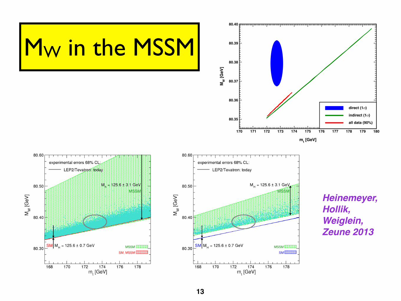
Figure 6: Prediction for MW as a function of mt. The left plot shows all points allowed byHiggsBounds, the middle one requires Mh to be in the mass region 125.6 ± 3.1 GeV, whilein the right plot MH is required to be in the mass region 125.6 ± 3.1 GeV. The color codingis as in Figs. 1 and 4. In addition, the blue points are the parameter points for which thestops and sbottoms are heavier than 500 GeV and squarks of the first two generations andthe gluino are heavier than 1200 GeV.
sleptons, charginos and neutralinos, as analyzed above.
While so far we have compared the various predictions with the current experimentalresults for MW and mt, we now discuss the impact of future improvements of these mea-surements. For the W boson mass we assume an improvement of a factor three comparedto the present case down to �MW = 5 MeV from future measurements at the LHC and aprospective Linear Collider (ILC) [118], while for mt we adopt the anticipated ILC accuracyof �mt = 100 MeV [119]. For illustration we show in Fig. 7 again the left plot of Fig. 4,assuming the mass of the light CP-even Higgs boson h in the region 125.6 ± 3.1 GeV, butsupplement the gray ellipse indicating the present experimental results for MW and mt withthe future projection indicated by the red ellipse (assuming the same experimental centralvalues). While currently the experimental results for MW and mt are compatible with thepredictions of both models (with a slight preference for a non-zero SUSY contribution), theanticipated future accuracies indicated by the red ellipse would clearly provide a high sen-sitivity for discriminating between the models and for constraining the parameter space ofBSM scenarios.
As a further hypothetical future scenario we assume that a light scalar top quark hasbeen discovered at the LHC with a mass of mt1
= 400 ± 40 GeV, while no other newparticle has been observed. As before, for this analysis we use an anticipated experimentalprecision of �MW = 5 MeV (other uncertainties have been neglected in this analysis).Concerning the masses of the other SUSY particles, we assume lower limits of 300 GeVon both sleptons and charginos, 500 GeV on other scalar quarks of the third generationand of 1200 GeV on the remaining colored particles. We have selected the points from our
19
�13
Heinemeyer, Hollik, Weiglein, Zeune 2013
MW in the MSSM
170 171 172 173 174 175 176 177 178 179 180
mt [GeV]
80.35
80.36
80.37
80.38
80.39
80.40
MW
[GeV
]
direct (1σ)
indirect (1σ)
all data (90%)

mc
�14
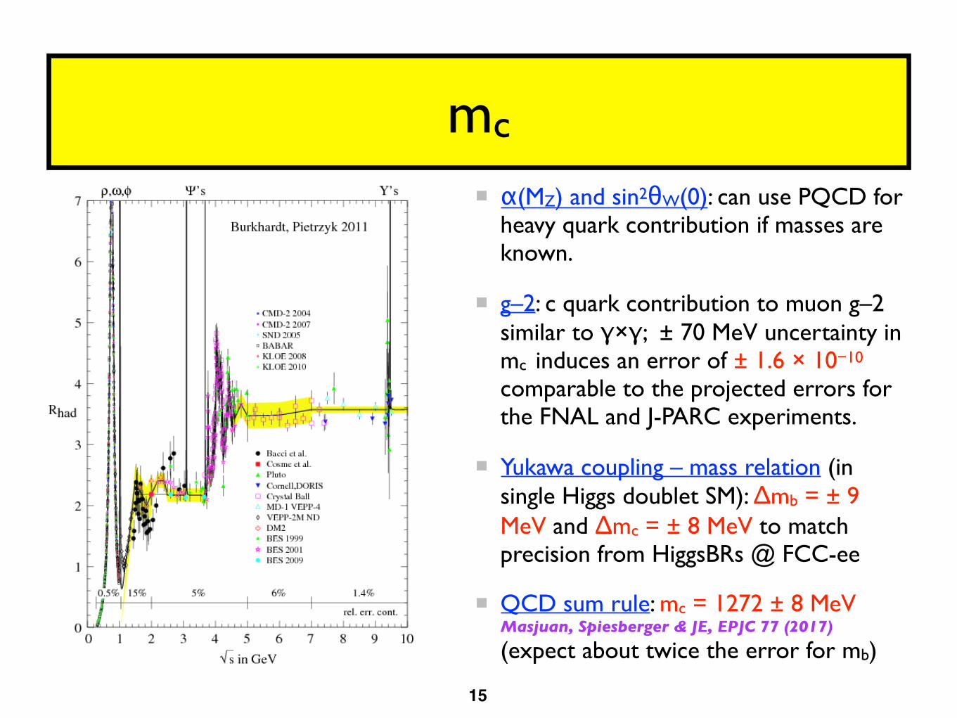
α(MZ) and sin2θW(0): can use PQCD for heavy quark contribution if masses are known.
g–2: c quark contribution to muon g–2 similar to γ×γ; ± 70 MeV uncertainty in mc induces an error of ± 1.6 × 10⁻¹⁰comparable to the projected errors for the FNAL and J-PARC experiments.
Yukawa coupling – mass relation (in single Higgs doublet SM): Δmb = ± 9 MeV and Δmc = ± 8 MeV to match precision from HiggsBRs @ FCC-ee
QCD sum rule: mc = 1272 ± 8 MeV Masjuan, Spiesberger & JE, EPJC 77 (2017) (expect about twice the error for mb)
mc
�15
α(MZ) and sin2θW(0): can use PQCD for heavy quark contribution if masses are known.
g–2: c quark contribution to muon g–2 similar to γ×γ; ± 70 MeV uncertainty in mc induces an error of ± 1.6 × 10⁻¹⁰comparable to the projected errors for the FNAL and J-PARC experiments.
Yukawa coupling – mass relation (in single Higgs doublet SM): Δmb = ± 9 MeV and Δmc = ± 8 MeV to match precision from HiggsBRs @ FCC-ee
QCD sum rule: mc = 1272 ± 8 MeV Masjuan, Spiesberger & JE, EPJC 77 (2017) (expect about twice the error for mb)

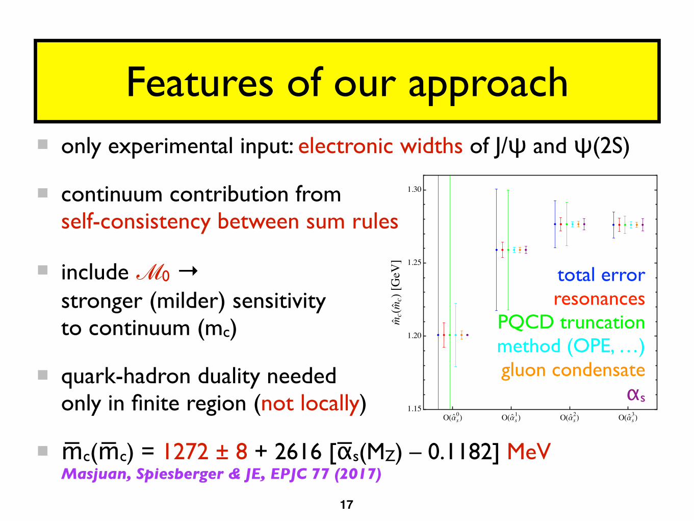
only experimental input: electronic widths of J/ψ and ψ(2S)
continuum contribution from self-consistency between sum rules
include ℳ0 → stronger (milder) sensitivity to continuum (mc)
quark-hadron duality neededonly in finite region (not locally)
mc(mc) = 1272 ± 8 + 2616 [αs(MZ) – 0.1182] MeVMasjuan, Spiesberger & JE, EPJC 77 (2017)
2.0 2.5 3.0 3.5 4.0 4.5 5.02.0
2.5
3.0
3.5
4.0
4.5
5.0
s @GeVD
RHsL 3.74 3.76 3.78 3.80 3.82
2.02.53.03.54.04.5
Features of our approach
�16
only experimental input: electronic widths of J/ψ and ψ(2S)
continuum contribution from self-consistency between sum rules
include ℳ0 → stronger (milder) sensitivity to continuum (mc)
quark-hadron duality neededonly in finite region (not locally)
mc(mc) = 1272 ± 8 + 2616 [αs(MZ) – 0.1182] MeVMasjuan, Spiesberger & JE, EPJC 77 (2017)
Features of our approach
�17
OHas0L OHas1L OHas2L OHas3L1.15
1.20
1.25
1.30
mcHm
cL@GeVD
total errorresonances
PQCD truncationmethod (OPE, …) gluon condensate
αs

Gauge Couplings at Lower Energies

ττ result includes leptonic branching ratios
ℬτs = 0.0292 ± 0.0004 (∆S = –1) PDG 2018
S(mτ, MZ) = 1.01907 ± 0.0003 JE, Rev. Mex. Fis. 50 (2004)
δNP = 0.003 ± 0.009 (within OPE & OPE breaking) based on (controversial) Boito et al., PRD 85 (2012) & PRD 91 (2015); Davier et al., EPJC 74 (2014); Pich & Rodríguez-Sánchez, PRD 94 (2016)
αs from τ decays
�19
1. Electroweak model and constraints on new physics 23
of new physics contributions. By far the most precise observable discussed here is theanomalous magnetic moment of the muon (the electron magnetic moment is measured toeven greater precision and can be used to determine α, but its new physics sensitivity issuppressed by an additional factor of m2
e/m2µ, unless there is a new light degree of freedom
such as a dark Z [165] boson). Its combined experimental and theoretical uncertainty iscomparable to typical new physics contributions.
The extraction of αs from the τ lifetime [166] is standing out from other determinationsbecause of a variety of independent reasons: (i) the τ -scale is low, so that uponextrapolation to the Z scale (where it can be compared to the theoretically cleanZ lineshape determinations) the αs error shrinks by about an order of magnitude;(ii) yet, this scale is high enough that perturbation theory and the operator productexpansion (OPE) can be applied; (iii) these observables are fully inclusive and thus freeof fragmentation and hadronization effects that would have to be modeled or measured;(iv) duality violation (DV) effects are most problematic near the branch cut but therethey are suppressed by a double zero at s = m2
τ ; (v) there are data [37,167] to constrainnon-perturbative effects both within and breaking the OPE; (vi) a complete four-looporder QCD calculation is available [160]; (vii) large effects associated with the QCDβ-function can be re-summed [168] in what has become known as contour improvedperturbation theory (CIPT). However, while there is no doubt that CIPT shows fasterconvergence in the lower (calculable) orders, doubts have been cast on the method by theobservation that at least in a specific model [169], which includes the exactly knowncoefficients and theoretical constraints on the large-order behavior, ordinary fixed orderperturbation theory (FOPT) may nevertheless give a better approximation to the fullresult. We therefore use the expressions [43,159,160,170],
ττ = !1 − Bs
τ
Γeτ + Γµ
τ + Γudτ
= 290.75 ± 0.36 fs, (1.49)
Γudτ =
G2F m5
τ |Vud|2
64π3 S (mτ ,MZ)
!
1 +3
5
m2τ − m2
µ
M2W
"
×
#1 +
αs (mτ )
π+ 5.202
α2s
π2 + 26.37α3
s
π3 + 127.1α4
s
π4 +$απ
%85
24−
π2
2
&+ δNP
', (1.50)
and Γeτ and Γµ
τ can be taken from Eq. (1.6) with obvious replacements. The relativefraction of decays with ∆S = −1, Bs
τ = 0.0292 ± 0.0004, is based on experimentaldata since the value for the strange quark mass, $ms(mτ ), is not well known andthe QCD expansion proportional to $m2
s converges poorly and cannot be trusted.S(mτ ,MZ) = 1.01907 ± 0.0003 is a logarithmically enhanced EW correction factor withhigher orders re-summed [171]. δNP collects non-perturbative and quark-mass suppressedcontributions, including the dimension four, six and eight terms in the OPE, as well asDV effects. One group finds the slightly conflicting values δNP = −0.004± 0.012 [172] andδNP = 0.020 ± 0.009 [173], based on OPAL [37] and ALEPH [167] τ spectral functions,respectively. These can be combined to yield the average δNP = 0.0114± 0.0072. Another
April 8, 2018 22:12

dominant uncertainty from PQCD truncation(FOPT vs. CIPT vs. geometric continuation)
αS(4)(mτ) = 0.323+0.018–0.014
αS(5)(MZ) = 0.1184+0.0020–0.0018
updated from Luo & JE, PLB 558 (2003) in Freitas & JE (PDG 2018)
αs from τ decays
�20
1. Electroweak model and constraints on new physics 23
of new physics contributions. By far the most precise observable discussed here is theanomalous magnetic moment of the muon (the electron magnetic moment is measured toeven greater precision and can be used to determine α, but its new physics sensitivity issuppressed by an additional factor of m2
e/m2µ, unless there is a new light degree of freedom
such as a dark Z [165] boson). Its combined experimental and theoretical uncertainty iscomparable to typical new physics contributions.
The extraction of αs from the τ lifetime [166] is standing out from other determinationsbecause of a variety of independent reasons: (i) the τ -scale is low, so that uponextrapolation to the Z scale (where it can be compared to the theoretically cleanZ lineshape determinations) the αs error shrinks by about an order of magnitude;(ii) yet, this scale is high enough that perturbation theory and the operator productexpansion (OPE) can be applied; (iii) these observables are fully inclusive and thus freeof fragmentation and hadronization effects that would have to be modeled or measured;(iv) duality violation (DV) effects are most problematic near the branch cut but therethey are suppressed by a double zero at s = m2
τ ; (v) there are data [37,167] to constrainnon-perturbative effects both within and breaking the OPE; (vi) a complete four-looporder QCD calculation is available [160]; (vii) large effects associated with the QCDβ-function can be re-summed [168] in what has become known as contour improvedperturbation theory (CIPT). However, while there is no doubt that CIPT shows fasterconvergence in the lower (calculable) orders, doubts have been cast on the method by theobservation that at least in a specific model [169], which includes the exactly knowncoefficients and theoretical constraints on the large-order behavior, ordinary fixed orderperturbation theory (FOPT) may nevertheless give a better approximation to the fullresult. We therefore use the expressions [43,159,160,170],
ττ = !1 − Bs
τ
Γeτ + Γµ
τ + Γudτ
= 290.75 ± 0.36 fs, (1.49)
Γudτ =
G2F m5
τ |Vud|2
64π3 S (mτ ,MZ)
!
1 +3
5
m2τ − m2
µ
M2W
"
×
#1 +
αs (mτ )
π+ 5.202
α2s
π2 + 26.37α3
s
π3 + 127.1α4
s
π4 +$απ
%85
24−
π2
2
&+ δNP
', (1.50)
and Γeτ and Γµ
τ can be taken from Eq. (1.6) with obvious replacements. The relativefraction of decays with ∆S = −1, Bs
τ = 0.0292 ± 0.0004, is based on experimentaldata since the value for the strange quark mass, $ms(mτ ), is not well known andthe QCD expansion proportional to $m2
s converges poorly and cannot be trusted.S(mτ ,MZ) = 1.01907 ± 0.0003 is a logarithmically enhanced EW correction factor withhigher orders re-summed [171]. δNP collects non-perturbative and quark-mass suppressedcontributions, including the dimension four, six and eight terms in the OPE, as well asDV effects. One group finds the slightly conflicting values δNP = −0.004± 0.012 [172] andδNP = 0.020 ± 0.009 [173], based on OPAL [37] and ALEPH [167] τ spectral functions,respectively. These can be combined to yield the average δNP = 0.0114± 0.0072. Another
April 8, 2018 22:12

Dispersive approach:
α–1(MZ) = 128.947 ± 0.012 Davier et al., EPJC 77 (2017)
α–1(MZ) = 128.958 ± 0.016 Jegerlehner, arXiv:1711.06089
α–1(MZ) = 128.946 ± 0.015 Keshavarzi et al., arXiv:1802.02995
α–1(MZ) = 128.949 ± 0.010 Ferro-Hernández & JE, JHEP 03 (2018)
This value is converted from the MS scheme and uses both e+e– annihilation and τ decay spectral functions Davier et al., EPJC 77 (2017)
τ data corrected for γ-ρ mixing Jegerlehner & Szafron, EPJC 71 (2011)
PQCD for √s > 2 GeV (using mc & mb) Ferro-Hernández & JE, in preparation
α(MZ)
�21
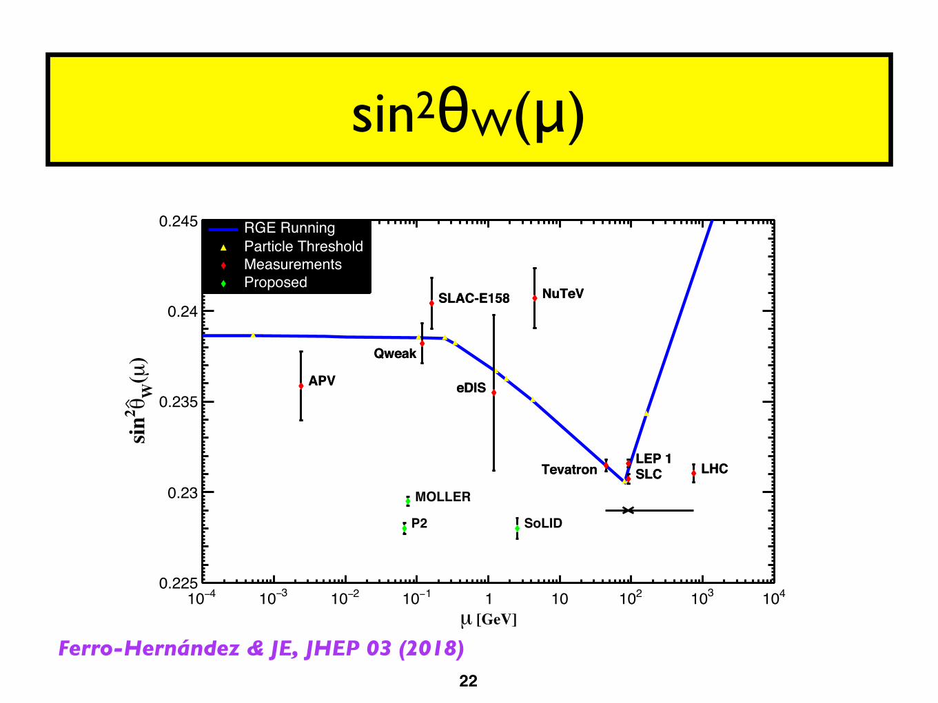
4−10 3−10 2−10 1−10 1 10 210 310 410 [GeV]µ
0.225
0.23
0.235
0.24
0.245
)µ(
Wθ2sin
LHC LEP 1 SLC Tevatron
eDIS
SLAC-E158
Qweak
APV
P2
MOLLER
SoLID
LHC LEP 1 SLC Tevatron
eDIS
SLAC-E158
Qweak
APV
RGE RunningParticle ThresholdMeasurementsProposed
sin2θW(μ)
�22
4−10 3−10 2−10 1−10 1 10 210 310 410 [GeV]µ
0.225
0.23
0.235
0.24
0.245
)µ(
Wθ2sin
LHC LEP 1 SLC Tevatron
NuTeV
eDIS
SLAC-E158
Qweak
APV
P2
MOLLER
SoLID
LHC LEP 1 SLC Tevatron
NuTeV
eDIS
SLAC-E158
Qweak
APV
RGE RunningParticle ThresholdMeasurementsProposed
Ferro-Hernández & JE, JHEP 03 (2018)
……. ……. …….

sin2θW(0): RGE
�23
JHEP03(2018)196
Energy range λ1 λ2 λ3 λ4
mt ≤ µ 920
28980
1455
920
MW ≤ µ < mt2144
625176
611
322
mb ≤ µ < MW2144
1522
51440
322
mτ ≤ µ < mb920
35
219
15
mc ≤ µ < mτ920
25
780
15
ms ≤ µ < mc12
12
536 0
md ≤ µ < ms920
25
13110
120
mu ≤ µ < md38
14
340 0
mµ ≤ µ < mu14 0 0 0
me ≤ µ < mµ14 0 0 0
Table 2. Coefficients entering the higher order RGE for the weak mixing angle.
with nq the number of active quarks and N ci = 3 the color factor for quarks. For leptons
one substitutes N ci = 1 and αs = 0, while Ki = 1 for bosons.
We can relate the RGE of α to that of sin2 θW since both, the γZ mixing tensor
ΠγZ and the photon vacuum polarization function Πγγ are pure vector-current correlators.
Including higher order corrections, the RGE for the Z boson vector coupling to fermion f ,
vf = Tf − 2Qf sin2 θW , where Tf is the third component of weak isospin of fermion f , is
then
µ2 dvfdµ2
=αQf
24π
!"
i
KiγiviQi + 12σ
#"
q
$#"
q
vq
$%. (2.4)
Eqs. (2.1) and (2.4) can be used [2] to obtain
s2(µ) = s2(µ0)α(µ)
α(µ0)+ λ1
&1− α(µ)
α(µ0)
'+
+α(µ)
π
&λ2
3ln
µ2
µ20
+3λ3
4ln
α(µ)
α(µ0)+ σ(µ0)− σ(µ)
', (2.5)
where the λi are known [2] constants given in table 2 and the explicit Ki dependence has
disappeared. The σ terms,
σ(µ) =λ4
33− 2nq
5
36
&(11− 24ζ3)
α2s(µ)
π2+ b
α3s(µ)
π3
', (2.6)
– 4 –
vf : Z vector coupling to fermion f
Ki : QCD factor known to O(αS4) Baikov et al., JHEP 07 (2012)
σ: singlet piece at O(αS3) and O(αS4) Baikov et al., JHEP 07 (2012)
γi : field type dependent constants Ramsey-Musolf & JE, PRD 72 (2005)
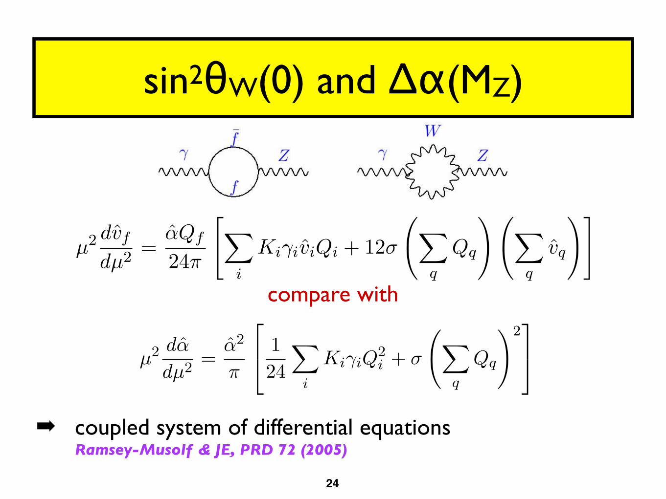
sin2θW(0) and Δα(MZ)
�24
JHEP03(2018)196
Energy range λ1 λ2 λ3 λ4
mt ≤ µ 920
28980
1455
920
MW ≤ µ < mt2144
625176
611
322
mb ≤ µ < MW2144
1522
51440
322
mτ ≤ µ < mb920
35
219
15
mc ≤ µ < mτ920
25
780
15
ms ≤ µ < mc12
12
536 0
md ≤ µ < ms920
25
13110
120
mu ≤ µ < md38
14
340 0
mµ ≤ µ < mu14 0 0 0
me ≤ µ < mµ14 0 0 0
Table 2. Coefficients entering the higher order RGE for the weak mixing angle.
with nq the number of active quarks and N ci = 3 the color factor for quarks. For leptons
one substitutes N ci = 1 and αs = 0, while Ki = 1 for bosons.
We can relate the RGE of α to that of sin2 θW since both, the γZ mixing tensor
ΠγZ and the photon vacuum polarization function Πγγ are pure vector-current correlators.
Including higher order corrections, the RGE for the Z boson vector coupling to fermion f ,
vf = Tf − 2Qf sin2 θW , where Tf is the third component of weak isospin of fermion f , is
then
µ2 dvfdµ2
=αQf
24π
!"
i
KiγiviQi + 12σ
#"
q
$#"
q
vq
$%. (2.4)
Eqs. (2.1) and (2.4) can be used [2] to obtain
s2(µ) = s2(µ0)α(µ)
α(µ0)+ λ1
&1− α(µ)
α(µ0)
'+
+α(µ)
π
&λ2
3ln
µ2
µ20
+3λ3
4ln
α(µ)
α(µ0)+ σ(µ0)− σ(µ)
', (2.5)
where the λi are known [2] constants given in table 2 and the explicit Ki dependence has
disappeared. The σ terms,
σ(µ) =λ4
33− 2nq
5
36
&(11− 24ζ3)
α2s(µ)
π2+ b
α3s(µ)
π3
', (2.6)
– 4 –
compare with
JHEP03(2018)196
boson γi fermion γi
real scalar 1 chiral fermion 4
complex scalar 2 Majorana fermion 4
massless gauge boson −22 Dirac fermion 8
Table 1. RGE contributions of different particle types, where the minus sign is indicative for theasymptotic freedom in non-Abelian gauge theories.
contains a brief discussion of various calculations of α(MZ)). Section 4 describes the
calculation of the singlet contribution to the weak mixing angle, with some details given in
appendix B. In section 5 the flavor separation (contributions of light and strange quarks)
is addressed and threshold masses are calculated. In section 6 theoretical uncertainties are
discussed in detail, and section 7 offers our final results and conclusions.
2 Renormalization group evolution
In an approximation in which all fermions are either massless and active or infinitely heavy
and decoupled, the RGE for the electromagnetic coupling in the MS scheme [24], α, can be
written in the form [2],
µ2 dα
dµ2=
α2
π
⎡
⎣ 1
24
∑
i
KiγiQ2i + σ
(∑
q
)2⎤
⎦ , (2.1)
where the sum is over all active particles in the relevant energy range. The Qi are the
electric charges, while the γi are constants depending on the field type and shown in
table 1. The Ki and σ contain higher-order corrections and are given by [25],
Ki = N ci
{1 +
3
4Q2
iα
π+
αs
π+
α2s
π2
[125
48− 11
72nq
]
+α3s
π3
[10487
1728+
55
18ζ3 − nq
(707
864+
55
54ζ3
)− 77
3888n2q
]
+α4s
4π4
[2665349
41472+
182335
864ζ3 −
605
16ζ4 −
31375
288ζ5
−nq
(11785
648+
58625
864ζ3 −
715
48ζ4 −
13325
432ζ5
)
−n2q
(4729
31104− 3163
1296ζ3 +
55
72ζ4
)+ n3
q
(107
15552+
1
108ζ3
)]}, (2.2)
and,
σ =α3s
π3
[55
216− 5
9ζ3
]+
α4s
π4
[11065
3456− 34775
3456ζ3 +
55
32ζ4 +
3875
864ζ5
− nq
(275
1728− 205
576ζ3 +
5
48ζ4 +
25
144ζ5
)], (2.3)
– 3 –
➡ coupled system of differential equations Ramsey-Musolf & JE, PRD 72 (2005)
sin2θW(0): result
�25
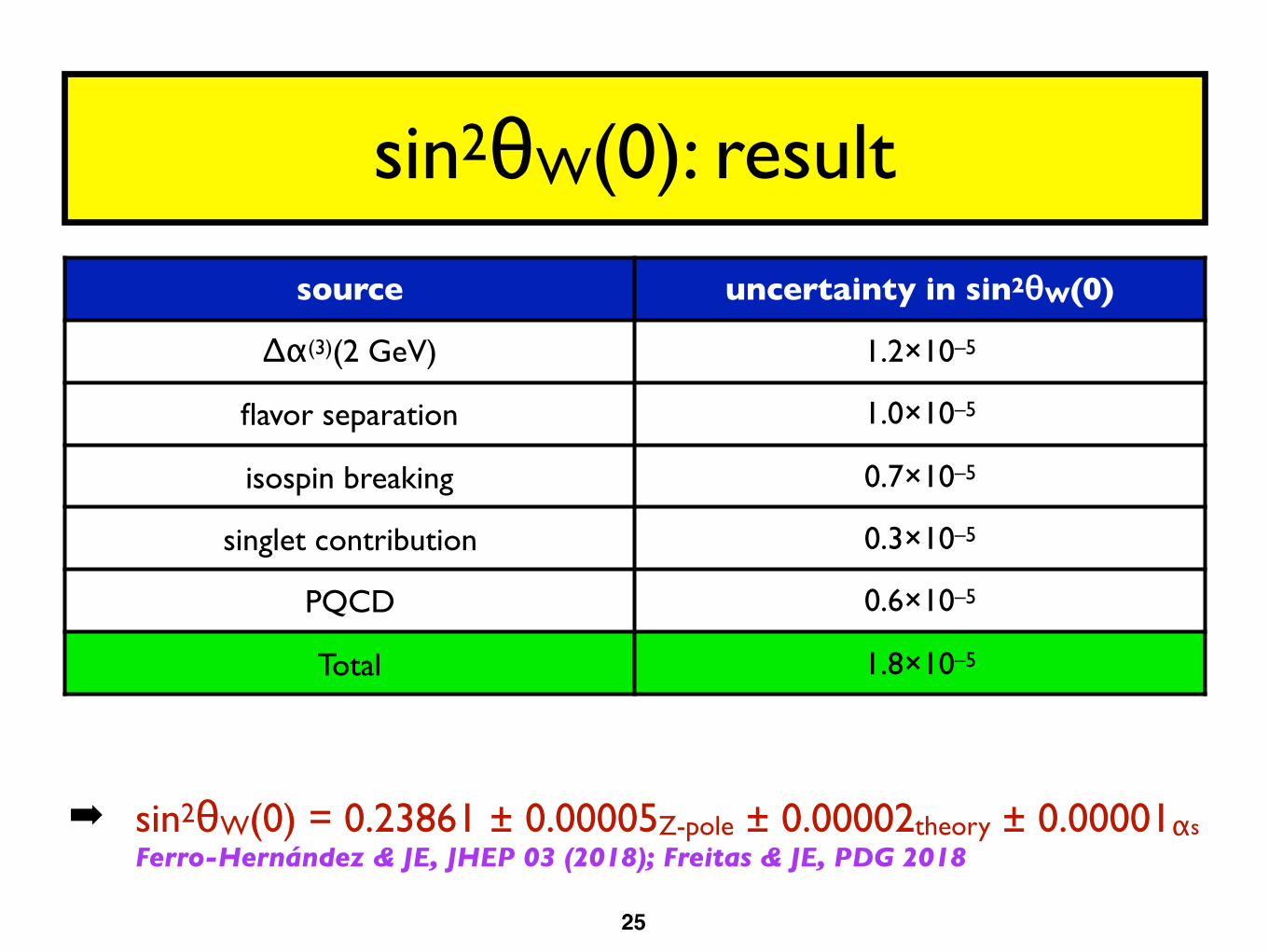
source uncertainty in sin2θW(0)
∆α(3)(2 GeV) 1.2×10⁻⁵
flavor separation 1.0×10⁻⁵
isospin breaking 0.7×10⁻⁵
singlet contribution 0.3×10⁻⁵
PQCD 0.6×10⁻⁵
Total 1.8×10⁻⁵
➡ sin2θW(0) = 0.23861 ± 0.00005Z-pole ± 0.00002theory ± 0.00001αs Ferro-Hernández & JE, JHEP 03 (2018); Freitas & JE, PDG 2018

Electroweak Fits
Performed with packageGlobal Analysis of Particle Properties
(GAPP)

Inputs
5 inputs needed to fix the bosonic sector of the SM: SU(3) × SU(2) × U(1) gauge couplings and 2 Higgs parameters
fine structure constant: α e.g. from the Rydberg constant (leaves ge–2 as derived quantity and extra SM test)
Fermi constant: GF from PSI (muon lifetime)
Z mass: MZ from LEP
Higgs mass: MH from the LHC
strong coupling constant: αs(MZ) is fit output ☛
�27

Standard global fit
�28
MH 125.14 ± 0.15 GeV
MZ 91.1884 ± 0.0020 GeV
mb(mb) 4.180 ± 0.021 GeV
∆αhad(3)(2 GeV) (59.0 ± 0.5)×10–4
mt(mt) 163.28 ± 0.44 GeV 1.00 –0.13 –0.28
mc(mc) 1.275 ± 0.009 GeV –0.13 1.00 0.45
αS(MZ) 0.1187 ± 0.0016 –0.28 0.45 1.00
other correlations small Freitas & JE, PDG 2018
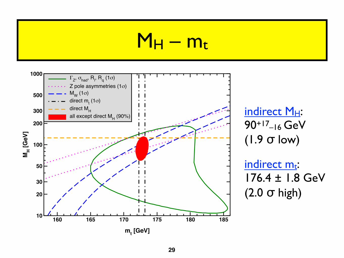
MH – mt
�29
160 165 170 175 180 185
mt [GeV]
10
20
30
50
100
200
300
500
1000
MH [G
eV]
ΓZ, σhad, Rl, Rq (1σ)Z pole asymmetries (1σ)MW (1σ)direct mt (1σ)direct MHall except direct MH (90%) indirect MH:
90+17–16 GeV (1.9 σ low)
indirect mt: 176.4 ± 1.8 GeV (2.0 σ high)

Oblique physics beyond the SM
STU describe corrections to gauge-boson self-energies
T breaks custodial SO(4)
a multiplet of heavy degenerate chiral fermions contributes ΔS = NC∕3π ∑i [t3Li − t3Ri]2
extra degenerate fermion family yields ΔS = 2∕3π ≈ 0.21
S and T (U) correspond to dimension 6 (8) operators�30�30
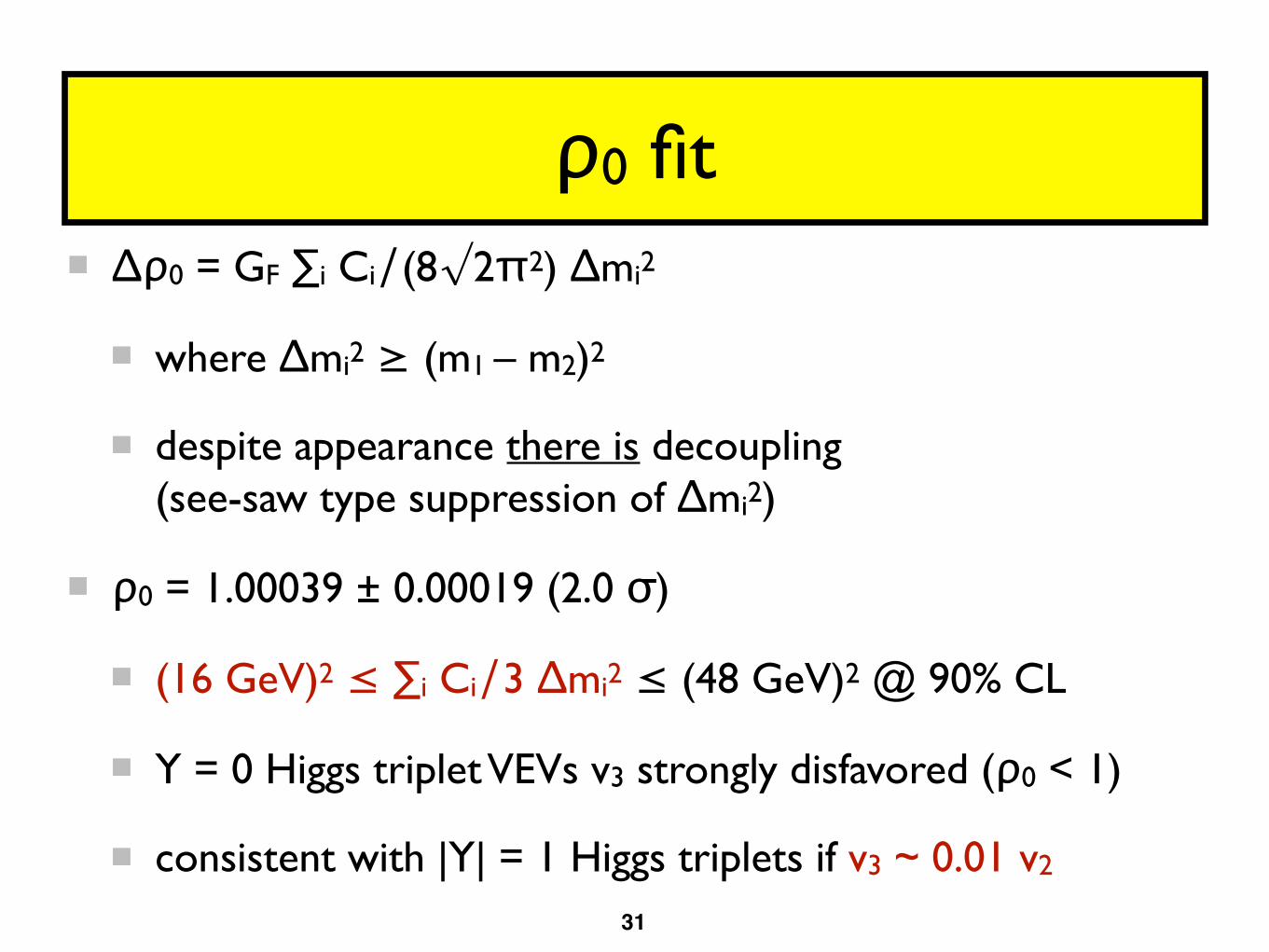
∆ρ0 = GF ∑i Ci∕(8√2π2) ∆mi2
where ∆mi2 ≥ (m1 – m2)2
despite appearance there is decoupling (see-saw type suppression of ∆mi2)
ρ0 = 1.00039 ± 0.00019 (2.0 σ)
(16 GeV)2 ≤ ∑i Ci∕3 ∆mi2 ≤ (48 GeV)2 @ 90% CL
Y = 0 Higgs triplet VEVs v3 strongly disfavored (ρ0 < 1)
consistent with |Y| = 1 Higgs triplets if v3 ~ 0.01 v2
ρ0 fit
�31

S parameter rules out QCD-like technicolor models
S also constrains extra degenerate fermion families:
➡ NF = 2.75 ± 0.14 (assuming T = U = 0)
compare with Nν = 2.991 ± 0.007 from ΓZ
S fit
�32

S and T
�33
-1.5 -1.0 -0.5 0 0.5 1.0 1.5S
-1.0
-0.5
0
0.5
1.0
T
ΓZ, σhad, Rl, Rq
asymmetriese & ν scatteringMW
APVall (90% CL)SM prediction
S 0.02 ± 0.07
T 0.06 ± 0.06
∆χ2 – 4.2
MKK ≳ 3.2 TeV in warped extra dimension models
MV ≳ 4 TeV in minimal composite Higgs models Freitas & JE (PDG 2018)

The SM is 50 years old and in great health — immortal?
ICHEP 2018: new ATLAS result based on 8 TeV data
sin2θW = 0.23140 ± 0.00036
agrees well with SM and world average
small tension in MW
surely only 2 σ … but in a very special observable
simplest possibility: ρ0 > 1
Precision in sin2θW (AFB) & MW and future polarized e– scattering experiments at low Q2 challenge theory → needs major global effort
Conclusions
�34

Backups
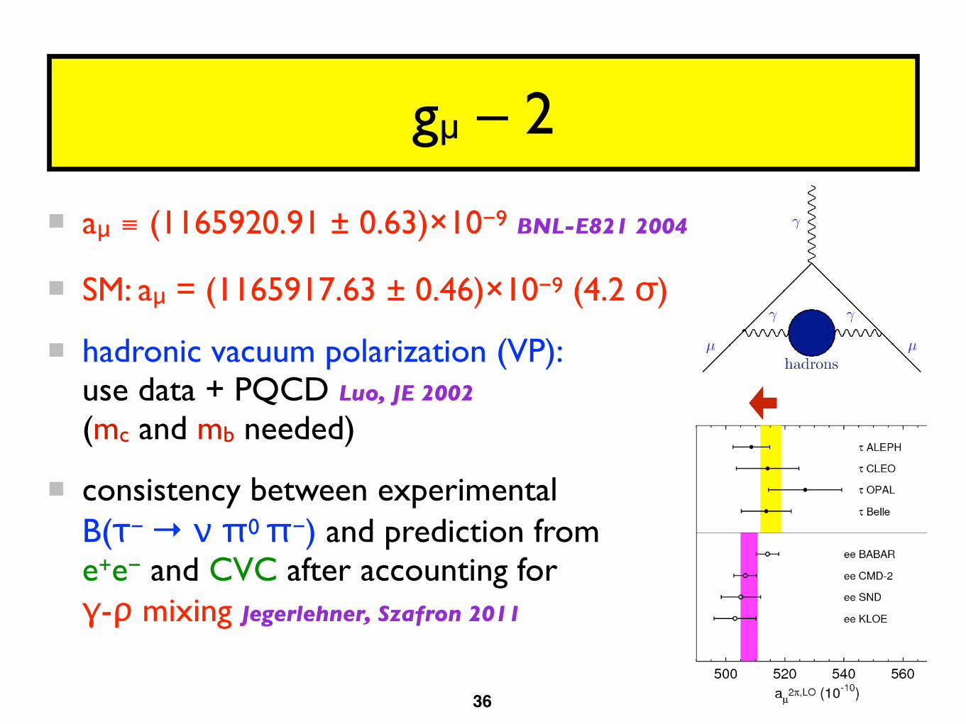
aμ ≡ (1165920.91 ± 0.63)×10−9 BNL-E821 2004
SM: aμ = (1165917.63 ± 0.46)×10−9 (4.2 σ)
hadronic vacuum polarization (VP): use data + PQCD Luo, JE 2002 (mc and mb needed)
consistency between experimental B(τ− → ν π0 π−) and prediction from e+e− and CVC after accounting for γ-ρ mixing Jegerlehner, Szafron 2011
�36
gµ – 2
�36
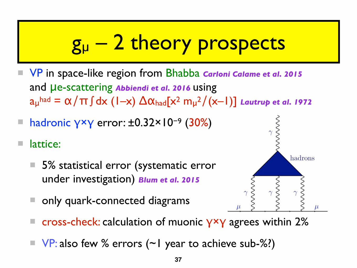
VP in space-like region from Bhabba Carloni Calame et al. 2015
and μe-scattering Abbiendi et al. 2016 using aμhad = α∕π∫dx (1–x) Δαhad[x2 mμ2∕(x–1)] Lautrup et al. 1972
hadronic γ×γ error: ±0.32×10⁻⁹ (30%)
lattice:
5% statistical error (systematic error under investigation) Blum et al. 2015
only quark-connected diagrams
cross-check: calculation of muonic γ×γ agrees within 2%
VP: also few % errors (~1 year to achieve sub-%?)�37
gµ – 2 theory prospects
�37

gμ–2 hadronic effects
�38
aμhad,LO = (69.31 ± 0.34)×10–9 Davier et al., EPJC 77 (2017)
aμhad,LO = (68.81 ± 0.41)×10–9 Jegerlehner, EPJ Web Conf. 166 (2018)
aμhad,LO = (68.88 ± 0.34)×10–9 (incl. τ data) Jegerlehner, EPJ Web Conf. 166 (2018)
aμhad,LO = (69.33 ± 0.25)×10–9 Keshavarzi et al., arXiv:1802.02995
aμhad,NLO = (–1.01 ± 0.01)×10–9 (anti-correlated with aμhad,LO) Krause, PLB 390 (1997)
aμhad,NNLO = (0.124 ± 0.001)×10–9 Kurz et al., EPJ Web Conf. 118 (2016)
aμhad,LBLS (α3) = (1.05 ± 0.33)×10–9 (mc treatment!) Toledo-Sánchez & JE, PRL 97 (2006)
aμhad,LBLS (α4) = (0.03 ± 0.02)×10–9 Colangelo et al., PLB 735 (2014)
aμ (exp.) – aμ (SM) = (2.55 ± 0.77)×10–9 (3.3 σ) Freitas & JE, PDG 2018

STU fit
�39
S 0.02 ± 0.10 1.00 0.92 –0.66
T 0.07 ± 0.12 0.92 1.00 –0.86
U 0.00 ± 0.09 –0.66 –0.86 1.00
sin2θW(MZ) 0.23113 ± 0.00014
αS(MZ) 0.1189 ± 0.0016
MKK ≳ 3.2 TeV in warped extra dimension models
MV ≳ 4 TeV in minimal composite Higgs models Freitas & JE (PDG 2018)
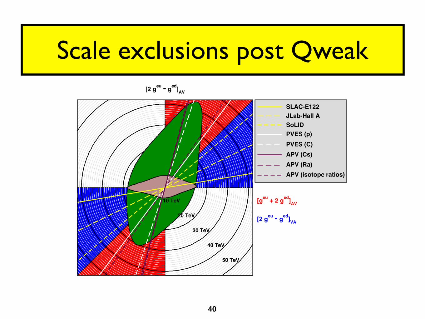
Scale exclusions post Qweak
�40
[2 geu - ged]AV
[geu + 2 ged]AV
[2 geu - ged]VA
10 TeV
20 TeV
30 TeV
40 TeV
50 TeV
SLAC-E122JLab-Hall ASoLIDPVES (p)PVES (C)APV (Cs)APV (Ra)APV (isotope ratios)

�41
-1 -0.9 -0.8 -0.7 -0.6 -0.5 -0.4 -0.3 -0.2 -0.1 0
[2 geu- ged]AV
0
0.1
0.2
0.3
0.4
0.5
0.6
0.7
0.8
0.9
1
[geu+ 2 ged]AV
APVQweakeDISall dataSM
-0.76 -0.74 -0.72 -0.70 -0.68
0.46
0.48
0.50
0.52
-1 -0.9 -0.8 -0.7 -0.6 -0.5 -0.4 -0.3 -0.2 -0.1 0
[2 geu- ged]AV
-0.5
-0.4
-0.3
-0.2
-0.1
0
0.1
0.2
0.3
0.4
0.5
[2 geu- ged]VA
Qweak + APVSLAC-E122JLab-Hall Aall dataSM
-0.76 -0.74 -0.72 -0.70 -0.68
-0.22
-0.20
-0.18
-0.16
-0.14
-0.12
-0.10
-0.08
[2 geu - ged]AV
[geu + 2 ged]AV
[2 geu - ged]VA
10 TeV
20 TeV
30 TeV
40 TeV
50 TeV
SLAC-E122JLab-Hall ASoLIDPVES (p)PVES (C)APV (Cs)APV (Ra)APV (isotope ratios)
Compositenessscales from
low energies
�41

Scale exclusions pre-SoLID / P2
�42
[2 geu - ged]AV
[2 geu - ged]VA
10 TeV
20 TeV
30 TeV
40 TeV
50 TeV
JLab-Hall ASoLIDSLAC-E122

Effective couplings
�43
-0.72 -0.715 -0.71 -0.705
[2 geu - ged]AV
0.485
0.49
0.495
0.5
[geu
+ 2
ged
] AV
P2 (1.7% H asymmetry)P2 (0.3% C asymmetry)2018 (all data)2018 + P2 (H target)2018 + P2 (H + C targets)Standard Model prediction
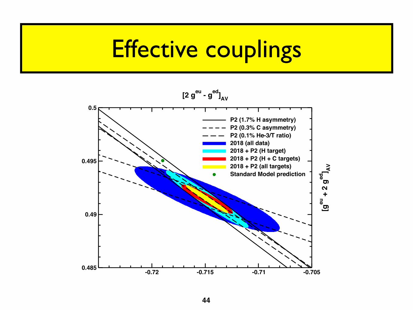
Effective couplings
�44
-0.72 -0.715 -0.71 -0.705
[2 geu - ged]AV
0.485
0.49
0.495
0.5
[geu
+ 2
ged
] AV
P2 (1.7% H asymmetry)P2 (0.3% C asymmetry)P2 (0.1% He-3/T ratio)2018 (all data)2018 + P2 (H target)2018 + P2 (H + C targets)2018 + P2 (all targets)Standard Model prediction

sin2θW(0): RGE solution
�45
λi : rational numbers depending on active particle content of the EFT
theory uncertainty from RGE running ~ 1.6×10⁻⁶ (negligible)
theory error from b and c matching ~ 3×10⁻⁶ (again using mc & mb)
we recycle the on-shell result for α(2 GeV) Davier et al., EPJC 77 (2017)
→ scheme conversion introducing 4.8×10⁻⁶ uncertainty
total uncertainty from PQCD ~ 6×10⁻⁶ in sin2θW(0) ≡ s2
JHEP03(2018)196
Energy range λ1 λ2 λ3 λ4
mt ≤ µ 920
28980
1455
920
MW ≤ µ < mt2144
625176
611
322
mb ≤ µ < MW2144
1522
51440
322
mτ ≤ µ < mb920
35
219
15
mc ≤ µ < mτ920
25
780
15
ms ≤ µ < mc12
12
536 0
md ≤ µ < ms920
25
13110
120
mu ≤ µ < md38
14
340 0
mµ ≤ µ < mu14 0 0 0
me ≤ µ < mµ14 0 0 0
Table 2. Coefficients entering the higher order RGE for the weak mixing angle.
with nq the number of active quarks and N ci = 3 the color factor for quarks. For leptons
one substitutes N ci = 1 and αs = 0, while Ki = 1 for bosons.
We can relate the RGE of α to that of sin2 θW since both, the γZ mixing tensor
ΠγZ and the photon vacuum polarization function Πγγ are pure vector-current correlators.
Including higher order corrections, the RGE for the Z boson vector coupling to fermion f ,
vf = Tf − 2Qf sin2 θW , where Tf is the third component of weak isospin of fermion f , is
then
µ2 dvfdµ2
=αQf
24π
!"
i
KiγiviQi + 12σ
#"
q
$#"
q
vq
$%. (2.4)
Eqs. (2.1) and (2.4) can be used [2] to obtain
s2(µ) = s2(µ0)α(µ)
α(µ0)+ λ1
&1− α(µ)
α(µ0)
'+
+α(µ)
π
&λ2
3ln
µ2
µ20
+3λ3
4ln
α(µ)
α(µ0)+ σ(µ0)− σ(µ)
', (2.5)
where the λi are known [2] constants given in table 2 and the explicit Ki dependence has
disappeared. The σ terms,
σ(µ) =λ4
33− 2nq
5
36
&(11− 24ζ3)
α2s(µ)
π2+ b
α3s(µ)
π3
', (2.6)
– 4 –

use of result for α(2 GeV) needs singlet piece isolation ∆disc α(2 GeV)
then ∆disc s2 = (s2 ± 1∕20) ∆disc α(2 GeV) = (– 6 ± 3)×10–6
step function ⇒ singlet threshold mass msdisc ≈ 350 MeV
sin2θW(0): singlet separation
�46
JHEP03(2018)196
Figure 1. Examples of a connected (top) and a disconnected (bottom) Feynman diagram.
and bottom quark vector-current correlators amount to about 9 × 10⁻⁶ and −9 × 10⁻⁶,
respectively. Taking these as conservative bounds on the unknown higher-order terms and
combining them in quadrature results in an estimated truncation error of ±1.3×10⁻⁵ in α.
The matching conditions of s2 and α can also be related [2],
sin2 θW (mf )− =
α(mf )−
α(mf )+sin2 θW (mf )
+ +QiTi
2Q2i
!1−
α(mf )−
α(mf )+
". (2.9)
Applying the numerical analysis of the previous paragraph to eq. (2.9), we find 2.4× 10⁻⁶
and −1.4× 10⁻⁶, respectively, and we estimate a truncation error related to the matching
of about ±3× 10⁻⁶ in s2.
For completeness we recall that integrating out the W± bosons induces the one-loop
matching condition [2, 28],1
α+=
1
α− +1
6π. (2.10)
For s2 this implies
sin2 θW (MW )+ = 1− α(MW )+
α(MW )−cos2 θW (MW )−. (2.11)
3 Implementation of experimental input
The perturbative treatment of the previous section cannot be applied at hadronic energy
scales and experimental input is required. This is usually taken from R(s), i.e., the cross
section σ(e+e− → hadrons) normalized to σ(e+e− → µ+µ−). Additional information on
R(s) is encoded in hadronic τ decay spectral functions [32]. The traditional method to
– 6 –
JHEP03(2018)196
Figure 2. Scale dependence of the singlet contribution to ∆α (solid line) and its step functionapproximation (dashed line).
in the perturbative regime. Also shown in figure 2 is the step function approximation of
∆discα(q), with the step defined as the value of q where it reaches half of its asymptotic
value in eq. (4.10). We interpret this as the value where the strange quark decouples from
singlet diagrams, so that mdiscs ∼ 350MeV. Our central value of ms to be derived in the next
section, ms = 342MeV, is numerically very close to this providing evidence for mdiscs ≈ ms.
Eq. (4.9) and eq. (4.10) refer to quantities in the MS and on-shell schemes, respectively,
and in general these may differ. However, since we are working here in the three quark
theory and the sum of the charges of three light quarks vanishes, the change of schemes is
trivial. We can therefore use eq. (4.10) in eq. (4.9) and obtain,
∆discs2 = (−0.6± 0.3)× 10−5, (4.11)
where the uncertainty combines the errors from eq. (4.9) and the one induced by the lattice
calculation [23].
5 Flavor separation
In this section we perform a flavor separation of the contributions of up-type from down-
type quarks, or — given that up and down quarks are linked by the approximate strong
isospin symmetry — a separation of s from u and d quarks. Our strategy consists of
first using exclusively the experimental electro-production data as tabulated in ref. [16] to
constrain the contribution ∆sα of the strange quark to ∆α. We then exploit the lattice
gauge theory results in refs. [18, 19] to confirm and refine the purely data driven analysis.
Then we introduce the threshold mass mq of a quark q as the value of the ’t Hooft scale
where the QCD contribution to the corresponding decoupling relation becomes trivial. mc
and mb are treated in perturbation theory, while for u, d, and s quarks we derive bounds
using phenomenological and theoretical constraints.
– 10 –
Ferro-Hernández & JE, JHEP 03 (2018)adapted from lattice gμ–2 calculation
RBC/UKQCD, PRL 116 (2016)

use of result for α(2 GeV) also needs isolation of strange contribution ∆sα
left column assignment assumes OZI rule
expect right column to originate mostly from strange current (ms > mu,d)
quantify expectation using averaged ∆s(gμ–2) from lattices as Bayesian prior RBC/UKQCD, JHEP 04 (2016); HPQCD, PRD 89 (2014)
∆sα(1.8 GeV) = (7.09 ± 0.32)×10–4 (threshold mass ms = 342 MeV ≈ msdisc)
sin2θW(0): flavor separation
�47
strange quark external current ambiguous external current
Φ KK (non – Φ)
KKπ [almost saturated by Φ(1680)] KK2π, KK3π
ηΦ KKη, KKω