reinforcement learning, yet another introduction. part...
TRANSCRIPT
Reinforcement Learning,yet another introduction.
Part 2/3: Prediction problems
Emmanuel Rachelson (ISAE - SUPAERO)

Introduction Model-based prediction Monte-Carlo Temporal Differences TD(λ )
Quiz!
What’s an MDP?
{S,A,p, r ,T}Deterministic, Markovian, Stationary policies?
At least one is optimal
Evaluation equation?
Qπ(s,a) = r(s,a)+ γ ∑s′∈S
p(s′|s,π(s))Qπ(s′,π(s′))
Value Iteration?
Repeat Vn+1(s) = maxa∈A
{r(s,a)+ γ ∑
s′∈Sp(s′|s,a)V ∗n (s)
}
2 / 29

Introduction Model-based prediction Monte-Carlo Temporal Differences TD(λ )
Quiz!
What’s an MDP?
{S,A,p, r ,T}
Deterministic, Markovian, Stationary policies?
At least one is optimal
Evaluation equation?
Qπ(s,a) = r(s,a)+ γ ∑s′∈S
p(s′|s,π(s))Qπ(s′,π(s′))
Value Iteration?
Repeat Vn+1(s) = maxa∈A
{r(s,a)+ γ ∑
s′∈Sp(s′|s,a)V ∗n (s)
}
2 / 29

Introduction Model-based prediction Monte-Carlo Temporal Differences TD(λ )
Quiz!
What’s an MDP?
{S,A,p, r ,T}Deterministic, Markovian, Stationary policies?
At least one is optimal
Evaluation equation?
Qπ(s,a) = r(s,a)+ γ ∑s′∈S
p(s′|s,π(s))Qπ(s′,π(s′))
Value Iteration?
Repeat Vn+1(s) = maxa∈A
{r(s,a)+ γ ∑
s′∈Sp(s′|s,a)V ∗n (s)
}
2 / 29

Introduction Model-based prediction Monte-Carlo Temporal Differences TD(λ )
Quiz!
What’s an MDP?
{S,A,p, r ,T}Deterministic, Markovian, Stationary policies?
At least one is optimal
Evaluation equation?
Qπ(s,a) = r(s,a)+ γ ∑s′∈S
p(s′|s,π(s))Qπ(s′,π(s′))
Value Iteration?
Repeat Vn+1(s) = maxa∈A
{r(s,a)+ γ ∑
s′∈Sp(s′|s,a)V ∗n (s)
}
2 / 29

Introduction Model-based prediction Monte-Carlo Temporal Differences TD(λ )
Challenge!
Estimate the travel time to D, when in A, B, C ?
3 / 29
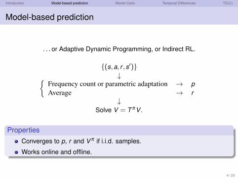
Introduction Model-based prediction Monte-Carlo Temporal Differences TD(λ )
Model-based prediction
. . . or Adaptive Dynamic Programming, or Indirect RL.
{(s,a, r ,s′)}↓{
Frequency count or parametric adaptation → pAverage → r
↓Solve V = T πV .
PropertiesConverges to p, r and V π if i.i.d. samples.
Works online and offline.
4 / 29
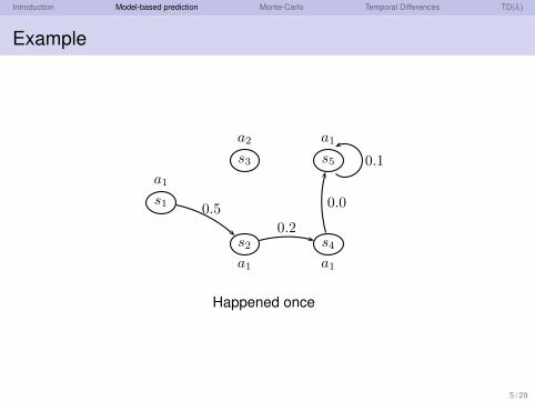
Introduction Model-based prediction Monte-Carlo Temporal Differences TD(λ )
Example
s1
s2
s3
s4
s5
a1
a1
a2
a1
a1
0.5
0.2
0.0
0.1
Happened once
5 / 29
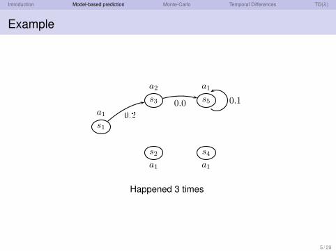
Introduction Model-based prediction Monte-Carlo Temporal Differences TD(λ )
Example
s1
s2
s3
s4
s5
a1
a1
a2
a1
a10.2 0.0 0.1
Happened 3 times
5 / 29
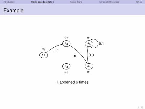
Introduction Model-based prediction Monte-Carlo Temporal Differences TD(λ )
Example
s1
s2
s3
s4
s5
a1
a1
a2
a1
a10.2 0.1 0.0
0.1
Happened 6 times
5 / 29
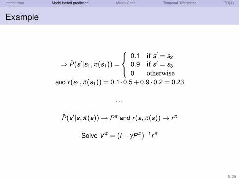
Introduction Model-based prediction Monte-Carlo Temporal Differences TD(λ )
Example
⇒ P̂(s′|s1,π(s1)) =
0.1 if s′ = s2
0.9 if s′ = s3
0 otherwiseand r(s1,π(s1)) = 0.1 ·0.5+0.9 ·0.2 = 0.23
. . .
P̂(s′|s,π(s))→ Pπ and r(s,π(s))→ rπ
Solve V π = (I− γPπ)−1rπ
5 / 29
Introduction Model-based prediction Monte-Carlo Temporal Differences TD(λ )
Model-based prediction
Incremental version: straightforward
Does not require full episodes for model updates
Requires maintaining a memory of the model
Has to be adapted for continuous domains
Requires many resolutions of V π = T πV π
6 / 29

Introduction Model-based prediction Monte-Carlo Temporal Differences TD(λ )
Question
And without a model ?
7 / 29
Introduction Model-based prediction Monte-Carlo Temporal Differences TD(λ )
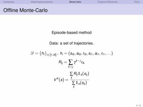
Offline Monte-Carlo
Episode-based method
Data: a set of trajectories.
D = {hi}i∈[1,N] , hi = (si0,ai0, ri0,si1,ai1, ri1, . . .)
Rij = ∑k≥j
γk−j rik
V π(s) =∑ij
Rij1s(sij)
∑ij1s(sij)
8 / 29
Introduction Model-based prediction Monte-Carlo Temporal Differences TD(λ )
Example
s1
s2
s3
s4
s5
a1
a1
a2
a1
a1
0.5
0.2
0.0
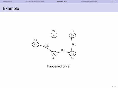
Happened once
9 / 29
Introduction Model-based prediction Monte-Carlo Temporal Differences TD(λ )
Example
s1
s2
s3
s4
s5
a1
a1
a2
a1
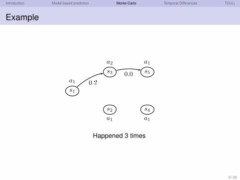
a10.2 0.0
Happened 3 times
9 / 29
Introduction Model-based prediction Monte-Carlo Temporal Differences TD(λ )
Example
s1
s2
s3
s4
s5
a1
a1
a2
a1
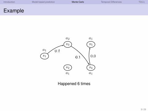
a10.2 0.1 0.0
Happened 6 times
9 / 29

Introduction Model-based prediction Monte-Carlo Temporal Differences TD(λ )
Example
V π(s3) =3 ·0.0+6 ·0.1
3+6=
115
9 / 29

Introduction Model-based prediction Monte-Carlo Temporal Differences TD(λ )
Offline Monte-Carlo
Requires finite-length episodes
Requires to remember full episodes
Online version ?
10 / 29

Introduction Model-based prediction Monte-Carlo Temporal Differences TD(λ )
Online Monte-Carlo
After each episode, update each encountered state’s value.Episode: h = (s0,a0, r0, . . .)
Rt = ∑i>t
γi−t rt
V π(st)← V π(st)+α [Rt −V π(st)]
11 / 29

Introduction Model-based prediction Monte-Carlo Temporal Differences TD(λ )
Example
Driving home!
12 / 29
Introduction Model-based prediction Monte-Carlo Temporal Differences TD(λ )
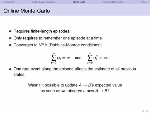
Online Monte-Carlo
Requires finite-length episodes.
Only requires to remember one episode at a time.
Converges to V π if (Robbins-Monroe conditions):
∞
∑t=0
αt = ∞ and∞
∑t=0
α2t < ∞.
One rare event along the episode affects the estimate of all previousstates.
Wasn’t it possible to update A→ D’s expected valueas soon as we observe a new A→ B?
13 / 29

Introduction Model-based prediction Monte-Carlo Temporal Differences TD(λ )
TD(0)
With each sample (st ,at , rt ,st+1):
V π(st)← V π(st)+α [rt + γV π(st+1)−V π(st)]
14 / 29

Introduction Model-based prediction Monte-Carlo Temporal Differences TD(λ )
Example
Driving home!
15 / 29
Introduction Model-based prediction Monte-Carlo Temporal Differences TD(λ )
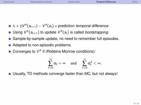
rt + γV π(st+1)−V π(st) = prediction temporal difference
Using V π(st+1) to update V π(st) is called bootstrapping
Sample-by-sample update, no need to remember full episodes.
Adapted to non-episodic problems.
Converges to V π if (Robbins-Monroe conditions):
∞
∑t=0
αt = ∞ and∞
∑t=0
α2t < ∞.
Usually, TD methods converge faster than MC, but not always!
16 / 29

Introduction Model-based prediction Monte-Carlo Temporal Differences TD(λ )
TD(λ )
Can we have the advantages of both MC and TD methods?
What’s inbetween TD and MC?
TD(0): 1-sample update with bootstrappingMC: ∞-sample update no bootstrapping
inbetween: n-sample update with bootstrapping
17 / 29
Introduction Model-based prediction Monte-Carlo Temporal Differences TD(λ )
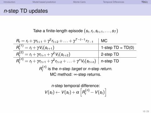
n-step TD updates
Take a finite-length episode (st , rt ,st+1, . . . ,sT )
Rt = rt + γrt+1 + γ2rt+2 + . . .+ γT−t−1rT−1 MC
R(1)t = rt + γVt(st+1) 1-step TD = TD(0)
R(2)t = rt + γrt+1 + γ2Vt(st+2) 2-step TD
R(n)t = rt + γrt+1 + γ2rt+2 + . . .+ γnVt(st+n) n-step TD
R(n)t is the n-step target or n-step return.
MC method: ∞-step returns.
n-step temporal difference:
V (st)← V (st)+α
[R(n)
t −V (st)]
18 / 29

Introduction Model-based prediction Monte-Carlo Temporal Differences TD(λ )
n-step TD updates
Converge to the true V π , just like TD(0) and MC methods.
Needs to wait for n steps to perform updates.
Not really used but useful for what follows.
19 / 29

Introduction Model-based prediction Monte-Carlo Temporal Differences TD(λ )
Mixing n-step and m-step returns
Consider Rmixt = 1
3 R(2)t + 2
3 R(4)t .
V (st)← V (st)+α[Rmix
t −V (st)]
Converges to V π as long as the weights sum to 1!
20 / 29

Introduction Model-based prediction Monte-Carlo Temporal Differences TD(λ )
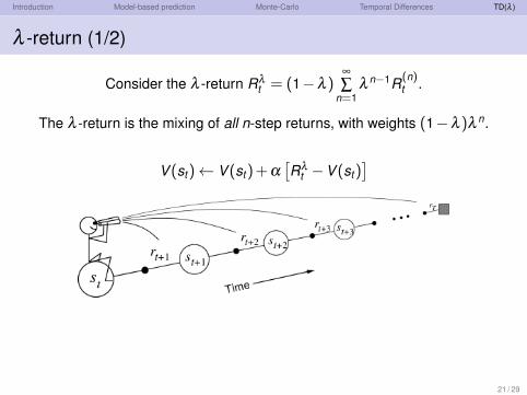
λ -return (1/2)
Consider the λ -return Rλt = (1−λ )
∞
∑n=1
λ n−1R(n)t .
The λ -return is the mixing of all n-step returns, with weights (1−λ )λ n.
21 / 29
Introduction Model-based prediction Monte-Carlo Temporal Differences TD(λ )
λ -return (1/2)
Consider the λ -return Rλt = (1−λ )
∞
∑n=1
λ n−1R(n)t .
The λ -return is the mixing of all n-step returns, with weights (1−λ )λ n.
V (st)← V (st)+α[Rλ
t −V (st)]
21 / 29

Introduction Model-based prediction Monte-Carlo Temporal Differences TD(λ )
λ -return (1/2)
Consider the λ -return Rλt = (1−λ )
∞
∑n=1
λ n−1R(n)t .
The λ -return is the mixing of all n-step returns, with weights (1−λ )λ n.
On a finite length episode of length T , ∀k > 0, R(T−t+k)t = Rt .
Rλt = (1−λ )
T−t−1
∑n=1
λn−1R(n)
t +(1−λ )∞
∑n=T−t
λn−1R(n)
t
= (1−λ )T−t−1
∑n=1
λn−1R(n)
t +(1−λ )λT−t−1
∞
∑n=T−t
λn−T+tR(n)
t
= (1−λ )T−t−1
∑n=1
λn−1R(n)
t +(1−λ )λT−t−1
∞
∑k=0
λk R(T−t+k)
t
= (1−λ )T−t−1
∑n=1
λn−1R(n)
t +λT−t−1Rt
21 / 29
Introduction Model-based prediction Monte-Carlo Temporal Differences TD(λ )
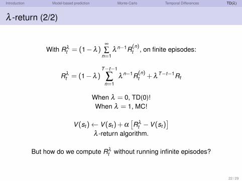
λ -return (2/2)
With Rλt = (1−λ )
∞
∑n=1
λ n−1R(n)t , on finite episodes:
Rλt = (1−λ )
T−t−1
∑n=1
λn−1R(n)
t +λT−t−1Rt
When λ = 0, TD(0)!When λ = 1, MC!
V (st)← V (st)+α[Rλ
t −V (st)]
λ -return algorithm.
But how do we compute Rλt without running infinite episodes?
22 / 29

Introduction Model-based prediction Monte-Carlo Temporal Differences TD(λ )
Eligibility traces
Eligibity trace of state s: et(s).
et(s) =
{γλet−1(s) if s 6= st
γλet−1(s)+1 if s = st
If no visit to a state, exponential decay.
→ et(s) measures how old the last visit to s is.
23 / 29
Introduction Model-based prediction Monte-Carlo Temporal Differences TD(λ )
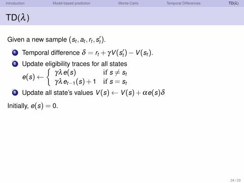
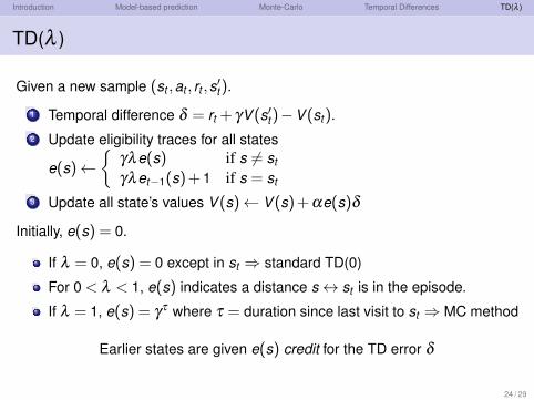
TD(λ )
Given a new sample (st ,at , rt ,s′t).
1 Temporal difference δ = rt + γV (s′t)−V (st).2 Update eligibility traces for all states
e(s)←{
γλe(s) if s 6= st
γλet−1(s)+1 if s = st
3 Update all state’s values V (s)← V (s)+αe(s)δ
Initially, e(s) = 0.
If λ = 0, e(s) = 0 except in st ⇒ standard TD(0)
For 0 < λ < 1, e(s) indicates a distance s↔ st is in the episode.
If λ = 1, e(s) = γτ where τ = duration since last visit to st ⇒ MC method
Earlier states are given e(s) credit for the TD error δ
24 / 29
Introduction Model-based prediction Monte-Carlo Temporal Differences TD(λ )
TD(λ )
Given a new sample (st ,at , rt ,s′t).
1 Temporal difference δ = rt + γV (s′t)−V (st).2 Update eligibility traces for all states
e(s)←{
γλe(s) if s 6= st
γλet−1(s)+1 if s = st
3 Update all state’s values V (s)← V (s)+αe(s)δ
Initially, e(s) = 0.
If λ = 0, e(s) = 0 except in st ⇒ standard TD(0)
For 0 < λ < 1, e(s) indicates a distance s↔ st is in the episode.
If λ = 1, e(s) = γτ where τ = duration since last visit to st ⇒ MC method
Earlier states are given e(s) credit for the TD error δ
24 / 29

Introduction Model-based prediction Monte-Carlo Temporal Differences TD(λ )
TD(1)
TD(1) implements Monte Carlo estimation on non-episodic problems!
TD(1) learns incrementally for the same result as MC
25 / 29
Introduction Model-based prediction Monte-Carlo Temporal Differences TD(λ )
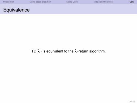
Equivalence
TD(λ ) is equivalent to the λ -return algorithm.
26 / 29
Introduction Model-based prediction Monte-Carlo Temporal Differences TD(λ )
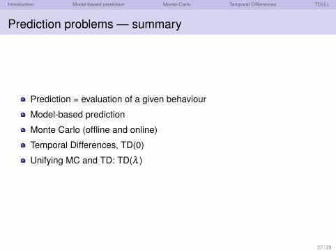
Prediction problems — summary
Prediction = evaluation of a given behaviour
Model-based prediction
Monte Carlo (offline and online)
Temporal Differences, TD(0)
Unifying MC and TD: TD(λ )
27 / 29

Introduction Model-based prediction Monte-Carlo Temporal Differences TD(λ )
Going further
Best value of λ?
Other variants?
Very large state spaces?
Continuous state spaces?
Value function approximation?
28 / 29

Introduction Model-based prediction Monte-Carlo Temporal Differences TD(λ )
Next class
Control
1 Online problems1 Q-learning2 SARSA
2 Offline learning1 (fitted) Q-iteration2 (least squares) Policy Iteration
29 / 29