relative astrometry and orbit determination

Madeleine Burheim

Lund ObservatoryLund University

Relative Astrometry andOrbit Determination

Degree project of 15 higher education creditsJune 2014

Supervisor: David Hobbs

Lund ObservatoryBox 43SE-221 00 LundSweden

2014-EXA88

Populärvetenskaplig sammanfattning

Att bestämma omloppsbanan för en komet kan svara på många frågor om vårt solsystem, och även resten av universum. Idag använder vi oss av olika algoritmer för att preliminärt kunna beräkna omloppsbanor hos bland annat kometer, men vad krävs egentligen för att få ett någorlunda korrekt resultat? Det finns ett antal olika metoder för att bestämma omloppsbanan hos en komet, men alla är grundade i den äldsta grenen av astronomin; astrometri, vars syfte är att mäta positioner och rörelser hos olika himlakroppar. Astrometrin sträcker sig långt före Galileos tid och har utvecklats avsevärt genom åren. Idag använder vi särskilda satelliter avsedda för att samla in information om bl. a kometer, vilket är vad en stor del av detta projekt kommer handla om.

Den metod jag har använt mig av för att beräkna omloppsbana för en komet är den så kallade Gauss metoden. Denna metod går ut på att vi känner till kometens position vid tre olika datum och därifrån, genom ett datorprogram, beräknar banans parametrar, kometens så kallade banelement. För mindre än tre kända datum fungerar inte denna metod, men det är även viktigt att vi använder ”rätt” datum. Väljer vi datum med för liten separation kommer vårt resultat inte att bli särskilt korrekt. Vi måste alltså använda datum med större separation för att få ett så bra resultat som möjligt på våra banelement.

I rapporten har jag upprepat processen för två aktuella kometer; C/2011 L4 PANSTARRS och C/2012 S1 ISON, för vilka jag i sin tur har beräknat banelementen utifrån olika kända datum. De resultat jag fått fram för de båda kometernas banor har jag jämfört med värden från Minor Planet Center, för att få en uppfattning om kvaliteten av mina resultat, och hur det program jag använde hade kunnat förbättras och utvecklas.

Contents

1 An Introduction to Astrometry 11.1 Photographic Imaging and CCDs . . . . . . . . . . . . . . . . . . . . . . 31.2 Calibrations of Plates and CCDs . . . . . . . . . . . . . . . . . . . . . . 61.3 Least Squares Adjustment . . . . . . . . . . . . . . . . . . . . . . . . . . 71.4 The FOTO Program . . . . . . . . . . . . . . . . . . . . . . . . . . . . . 9

1.4.1 Results from the FOTO Program . . . . . . . . . . . . . . . . . . 9

2 Orbit Determination 122.1 Kepler and His Laws of Planetary Motions . . . . . . . . . . . . . . . . . 12

2.1.1 Kepler’s Equations . . . . . . . . . . . . . . . . . . . . . . . . . . 122.2 Determining an Orbit from Two Position Vectors . . . . . . . . . . . . . 15

2.2.1 The Sector-Triangle Ratio . . . . . . . . . . . . . . . . . . . . . . 152.3 Orbital Elements . . . . . . . . . . . . . . . . . . . . . . . . . . . . . . . 162.4 Methods for Determining the Orbit . . . . . . . . . . . . . . . . . . . . . 18

2.4.1 The Shortened Gauss Method . . . . . . . . . . . . . . . . . . . . 182.4.2 The Comprehensive Gaussian Procedure . . . . . . . . . . . . . . 19

3 Using the GAUSS Program to Obtain the Orbital Elements 223.1 Results from the GAUSS program . . . . . . . . . . . . . . . . . . . . . . 22

4 Concluding remarks 33

A Images of Comet PANSTARRS 35

B Images of Comet ISON 36

i

1 An Introduction to Astrometry

For more than two thousand years positions of celestial object have been measured, abranch within astronomy we call astrometry. Throughout history, astrometry has beenused within widely spread fields, from maritime navigation to the understanding of thescale of our solar system, and the motion of the Earth through space, and it provides themeans to a deeper understanding of the universe as a whole.

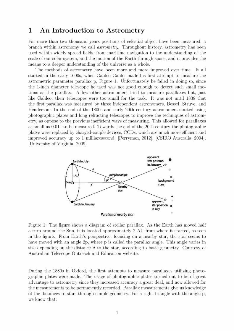
The methods of astrometry have been more and more improved over time. It allstarted in the early 1600s, when Galileo Galilei made his first attempt to measure theastrometric parameter parallax p, Figure 1. Unfortunately he failed in doing so, sincethe 1-inch diameter telescope he used was not good enough to detect such small mo-tions as the parallax. A few other astronomers tried to measure parallaxes but, justlike Galileo, their telescopes were too small for the task. It was not until 1838 thatthe first parallax was measured by three independent astronomers, Bessel, Struve, andHenderson. In the end of the 1800s and early 20th century astronomers started usingphotographic plates and long refracting telescopes to improve the techniques of astrom-etry, as oppose to the previous inefficient ways of measuring. This allowed for parallaxesas small as 0.01” to be measured. Towards the end of the 20th century the photographicplates were replaced by charged-couple devices, CCDs, which are much more efficient andimproved accuracy up to 1 milliarcsecond, [Perryman, 2012], [CSIRO Australia, 2004],[University of Virginia, 2009].

Figure 1: The figure shows a diagram of stellar parallax. As the Earth has moved halfa turn around the Sun, it is located approximately 2 AU from where it started, as seenin the figure. From Earth’s perspective, focusing on a nearby star, the star seems tohave moved with an angle 2p, where p is called the parallax angle. This angle varies insize depending on the distance d to the star, according to basic geometry. Courtesy ofAustralian Telescope Outreach and Education website.

During the 1880s in Oxford, the first attempts to measure parallaxes utilizing photo-graphic plates were made. The usage of photographic plates turned out to be of greatadvantage to astrometry since they increased accuracy a great deal, and now allowed forthe measurements to be permanently recorded. Parallax measurements give us knowledgeof the distances to stars through simple geometry. For a right triangle with the angle p,we know that:

1

sin p =1AU

d(1.1)

where 1 AU is the approximate average distance from Earth to the Sun, and d is thedistance to the star, as seen in figure 1. Since the distance to a star (other than ourSun), from the Earth, is very large, the intermediate angle, the parallax, becomes small.Using small-angle approximations for such an angle in radians, we get that sin p ≈ p.This means that our equation for small angles like parallaxes can be written as:

p =1

d[pc][′′]

where p is the parallax angle. Here the distance d is given in the astronomical unit parsec,pc, which is defined as the distance to a star with a parallax of one arcsecond. One parsecis approximately 3.3 light-years.

However, if we want to know how the stars move through space in relation to eachother we turn to another astrometric parameter, proper motion µ. Proper motion can beseen as the angular changes in the two coordinates right ascension α and declination δ,as follows,

µα = α′ − α µδ = δ′ − δ

where these two components can be combined into the total proper motion,

µ2 = µ2α + µ2

δ + cos2 δ (1.2)

However, years of observations of the motion of the wanted star, in relation to the back-ground stars, are required to calculate the proper motion of the star. One of the first todiscover the proper motion, in 1718, was the English scientist Edmund Halley. Compar-ing with older records of stellar position he noticed that some stars had moved slightlyrelative to the rest.

Astrometric observations are often used in our solar system, where it is mainly used totrack near-Earth objects. Images are taken regularly to make it possible to observe howa specific object in the solar system moves relative to the fixed stars in the background.

One type of near-Earth object constantly under observation are comets. Cometaryastronomy stretches back over two millennia to the times of ancient Greece and Rome, andeven further back to the Chaldeans of the Neo-Babylonian empire. However, comets havealways fascinated mankind and up until the 1700s they were regarded with superstitionand mysticism due to their, at the time, unpredictable motions and strange and varyingshapes. So far positional measurements had been made of comets and, when Newtondiscovered the law of gravity, these measurements could be used to accurately determinethe motions, orbits, distances, and even dimensions of these mysterious objects, as couldbe done for any of the celestial bodies. When the orbits of some comets had beendetermined it was clear that, just like the planets, these objects move around the Sun inorbits in the forms of the conic-sections.

In the early 19th century the unique and brilliant mathematician Carl Friedrich Gauss,who had developed a strong interest in astronomy, had gotten the idea of a new way ofdetermining the orbit of a comet or a planet. He applied his ideas for the first time ondetermining the orbit of Ceres using a set of three observations each time. His method

2

left a small residual error in the middle observation of each set, but these errors werewithout doubt smaller than those of his colleagues. To minimize the residuals Gaussapplied a so called least-squares adjustment to his calculated values, a numerical methodwhich will be described later in this document, [Vaccari, 2000], [Marsden, 1977].

A big breakthrough within astrometry was made in the late 1900s when the Hipparcossatellite (short for High Precision Parallax Collecting Satellite) was launched by theEuropean Space Agency (ESA). So far only ground based telescopes had been used forastrometric observations, but these were now facing barriers in improving the accuracyof the measurements. The main reason for these limitations was the effects of the Earth’satmosphere, other limitations were due to the gravitational and thermal impacts on theinstruments and the lack of an all-sky view. A solution to this problem was a space basedtelescope. The Hipparcos satellite operated between 1989 and 1993 and has revolutionizedthe field of astrometry, and thus astronomy as a whole. Hipparcos allowed for accuratedetermination of proper motions and parallaxes of stars, and thus determination of stellardistances.

A successor to Hipparcos is the The Gaia satellite, yet to be launched. Gaia originally anacronym for Global Astrometric Interferometer for Astrophysics, but due to redesign it nolonger uses interferometry for determining stellar positions and the acronym was dropped.Gaia will be used to make a 3D map of the Milky Way and give further information on theformation and evolution, and composition of the Galaxy. Gaia will, for a period of fiveyears, measure the physical properties, such as temperature, luminosity and composition,about 1% of all the stars in our Galaxy, as well as their positions and motions throughspace.

Global astrometry is used to measure positions and proper motions based on a singlefundamental reference frame for the whole sky. In global space astrometry we do notneed to consider the Earth’s rotation and orientation, the deformation and distortion ofthe surface of the earth, which much simplifies the problem. However, we do need toconsider the calibration of the telescope, and gravitational interaction of the solar systembodies, etc.

Differential astrometry is used to determine the position and motion of a celestial ob-ject over a smaller section of the sky relative to the surrounding objects, typically starslocated a few degrees away. The astrometric measurements, apart from position, arethe parallax, and proper motion. This project will be focused on differential astrometry,which is useful for measuring the orbits of comets [Festou et al., 1993].

In short, global astrometry is a “scan” of the whole sky, whereas differential astrom-etry only scans a section of the sky.

1.1 Photographic Imaging and CCDs

As mentioned above the simplified method to image the selected section of the sky usingphotographic plates has quite recently been replaced by the use of aCCD camera and apersonal computer, a method which makes it a lot easier to both take and store images.Nonetheless, in this section I will briefly explain the method of photographic plates, sincethe astrometric principle is the same for the two methods.

3

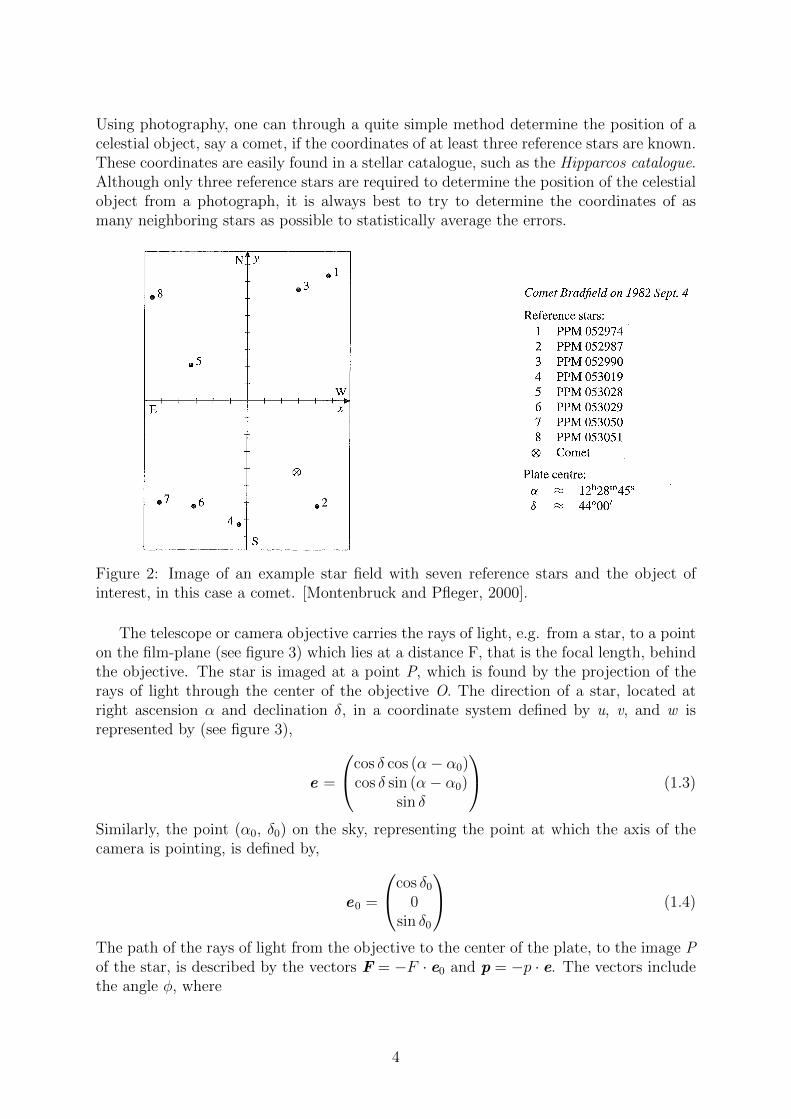
Using photography, one can through a quite simple method determine the position of acelestial object, say a comet, if the coordinates of at least three reference stars are known.These coordinates are easily found in a stellar catalogue, such as the Hipparcos catalogue.Although only three reference stars are required to determine the position of the celestialobject from a photograph, it is always best to try to determine the coordinates of asmany neighboring stars as possible to statistically average the errors.

Figure 2: Image of an example star field with seven reference stars and the object ofinterest, in this case a comet. [Montenbruck and Pfleger, 2000].

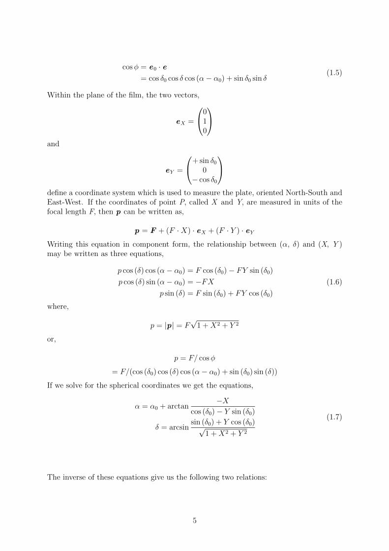
The telescope or camera objective carries the rays of light, e.g. from a star, to a pointon the film-plane (see figure 3) which lies at a distance F, that is the focal length, behindthe objective. The star is imaged at a point P, which is found by the projection of therays of light through the center of the objective O. The direction of a star, located atright ascension α and declination δ, in a coordinate system defined by u, v, and w isrepresented by (see figure 3),

e =

cos δ cos (α− α0)cos δ sin (α− α0)

sin δ

(1.3)

Similarly, the point (α0, δ0) on the sky, representing the point at which the axis of thecamera is pointing, is defined by,

e0 =

cos δ0

0sin δ0

(1.4)

The path of the rays of light from the objective to the center of the plate, to the image Pof the star, is described by the vectors F = −F · e0 and p = −p · e. The vectors includethe angle φ, where

4

cosφ = e0 · e= cos δ0 cos δ cos (α− α0) + sin δ0 sin δ

(1.5)

Within the plane of the film, the two vectors,

eX =

010

and

eY =

+ sin δ0

0− cos δ0

define a coordinate system which is used to measure the plate, oriented North-South andEast-West. If the coordinates of point P, called X and Y, are measured in units of thefocal length F, then p can be written as,

p = F + (F ·X) · eX + (F · Y ) · eYWriting this equation in component form, the relationship between (α, δ) and (X, Y )may be written as three equations,

p cos (δ) cos (α− α0) = F cos (δ0)− FY sin (δ0)

p cos (δ) sin (α− α0) = −FXp sin (δ) = F sin (δ0) + FY cos (δ0)

(1.6)

where,

p = |p| = F√

1 +X2 + Y 2

or,

p = F/ cosφ

= F/(cos (δ0) cos (δ) cos (α− α0) + sin (δ0) sin (δ))

If we solve for the spherical coordinates we get the equations,

α = α0 + arctan−X

cos (δ0)− Y sin (δ0)

δ = arcsinsin (δ0) + Y cos (δ0)√

1 +X2 + Y 2

(1.7)

The inverse of these equations give us the following two relations:

5

Figure 3: A chosen star field is represented on a photographic plate.The coordinates (α, δ) are translated into coordinates on the plate (X, Y ).[Montenbruck and Pfleger, 2000].

X = − cos (δ) sin (α− α0)

cos (δ0) cos (δ) cos (α− α0) + sin (δ0) sin (δ)

Y = −sin (δ0) cos (δ) cos (α− α0)− cos (δ0) sin (δ)

cos (δ0) cos (δ) cos (α− α0) + sin (δ0) sin (δ)

(1.8)

1.2 Calibrations of Plates and CCDs

X and Y are described as standard coordinates, since they are not dependent on the focallength of the employed optics. They refer to a system of coordinates which is orientedexactly parallel to the meridian that passes through the center of the photographic plate(α0, δ0). The measured coordinates x and y only have to be divided by the focal lengthF to obtain the standard coordinates, if this coordinate system is also to be used as thebasis for the plate reduction:

X = x/F

Y = y/F

After correcting for rotated axes, optical errors, possible tilt or distortion of the film, thestandard coordinates are generally expressed as:

X = a · x+ b · y + c

Y = d · x+ e · y + f(1.9)

where a, b, c, d, e, and f are known as the plate constants. These constants allowconversion between the (x, y) and (X, Y ) coordinates. The plate constants must bedetermined using reference stars. We need to know the equatorial coordinates (αi, δi)i=1,2,3

of at least three reference stars, giving us the following three equations:

6

X1 = x1 · a+ y1 · b+ c

X2 = x2 · a+ y2 · b+ c

X3 = x3 · a+ y3 · b+ c

(1.10)

in order to solve for a, b, and c. The same can be done for d, e, and f using the equationsfor Yi. Since measurements of stellar coordinates are never completely free from errors,we want to use as many reference stars as possible to determine the plate constants. Thisgives us a set of equations of the form:

X1 = x1 · a+ y1 · b+ c

. . .

Xn = xn · a+ yn · b+ c

(1.11)

where n > 3, for the three desired plate constants. However, this set of equations isoverdetermined and thus may not be solved uniquely. We therefore use a reductionprocedure called the least squares adjustment, in order to avoid this problem,[Montenbruck and Pfleger, 2000], [van Altena, 2013].

1.3 Least Squares Adjustment

For an overdetermined system, a system with more equations than unknowns, an approx-imate solution is needed. A method used to obtain such a solution is called the methodof least squares. Least squares is mostly used in data fitting and can be either linear ornon-linear, the first option is used in statistical regression analysis.

The goal of a least squares approximation is to minimize the difference between theactual observed value and the fit. These differences are called residuals and we writethem as (o - c), the observed value minus the calculated value, based on a model ofthe problem. We define the chi-squared equation as the residuals over the formal errors,summed over all i observations:

χ2 =n∑i=1

(o− cσ

)2 (1.12)

Writing the residuals into a vector y, we can express it with a matrix multiplication, asin the following equation:

Ax = y (1.13)

where A is our so called observation matrix, which describes how much the positionchanges on the plate/CCD if either the right ascension α or declination δ would beslightly altered. The x in our equation is a matrix which represents the change in rightascension and declination, which are our unknowns.

If the residuals, in eq 1.13, are minimized, that is when they are as close to zero aspossible, the unknowns can be obtained.

We now want to solve for x and this is done by multiplying with the transpose of thematrix A,

ATAx = ATy (1.14)

7

This gives a symmetric matrix known as the normal matrix, N, which we define asN = ATA, and b = ATy, so we can rewrite the equation as,

Nx = b (1.15)

From here it’s easier to solve for out unknowns x, which can now be written as,

x = N−1b (1.16)

which tells us how much the object has moved in right ascension and declination respec-tively. There are some standard algorithms for solving equation 1.14. Examples are SVD(Singular Value Decomposition), Cholesky decomposition, etc, [Tapley et al., 2004].

8

1.4 The FOTO Program

The FOTO program [Montenbruck and Pfleger, 2000] is a computer program, writtenin C++, which allows us to get fairly accurate positions of stars, comets, or minorplanets using photographic plates of the sky. Before actually using the program, someof the brighter stars will have been needed to be identified, with the help of a starchart. Although, in this thesis I have used the already chosen example reference stars,seen in [Montenbruck and Pfleger, 2000]. In this way, the approximate coordinates ofthe field that is covered by the plate can be determined. The equatorial coordinatesof the chosen reference stars may be found in a star catalogue, the one used in thisexample is the PPM (Position and Proper Motion) star catalogue. In order to help getmore accurate measurements the reference stars should be as point-like as possible, andevenly distributed throughout the plate. Now, to get the positions of the reference stars,as well as the object of interest, a transparent millimetre grid, oriented approximatelyNorth-South, is put over an enlargement of the image. Ultimately, to be able to calculatethe standard coordinates, the right ascension and declination of the plate center aredetermined. These values can be taken from a star atlas, since they are not required tobe completely accurate, given that errors in the coordinates of the plate center do nothave a big effect on position determination.

The known data are put into a data file Foto.dat, its first line containing the rightascension and declination of the plate center. After this follows details of the individualobjects on the plate, where reference stars which are to be used to determine the plateconstants are designate with an asterisk (*). After the name of the object, the measuredcoordinates x, y (in mm) are given. For the reference stars, also their equatorial coordi-nates α (h,m,s), δ (,’,”) are added. The Getinp function is used to read and store thesevalues, after which the standard coordinates of the reference stars are determined. Turn-ing this around, we can say that, the standard coordinates and the equatorial coordinatesof the objects on the plate are determined from the measured coordinates.

When the program is run we get our plate constants, a, b, c, d, e, and f, followed by theeffective focal length and the image scale. After these we get the measured coordinates(x, y) for all the objects, as well as the calculated standard coordinates (X, Y ) andthe equatorial coordinates, α and δ. The errors in the positions are also displayed (in”). Something that would be interesting to examine is whether it is possible to use anynumber of reference stars in the input file, and still get a stable result. Or, if the resultdecreases with decreasing number of reference stars and vice versa.

Repeated measurements over time give more values of the equatorial coordinates, α andδ, which can be used in order to calculate the parallax and proper motion of a celestialobject and determine its orbit around the Sun. This technique can be used to determinecometary orbits, provided that the plate constants for the photographic plate are knownalong with the measured coordinates of some reference stars. The program will thus giveus the standard coordinates for the comet as well as the equatorial coordinates, that areneeded when determining the orbit, which is the topic of the next section.

1.4.1 Results from the FOTO Program

As an example to show how this program works, I am using the example presented inAstronomy on the Personal Computer, 4th ed., by O. Montenbruck and T. Pfleger, 2000,[Montenbruck and Pfleger, 2000]. Here the goal is to obtain the equatorial coordinates

9

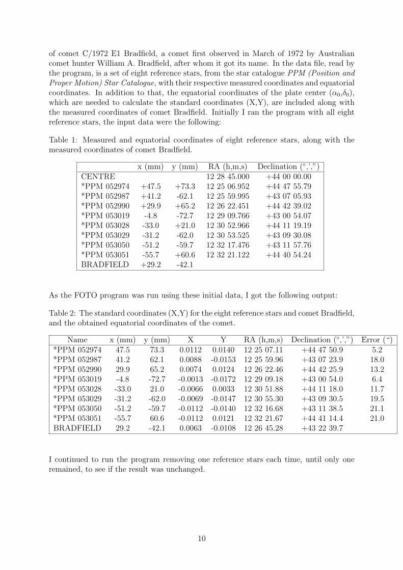
of comet C/1972 E1 Bradfield, a comet first observed in March of 1972 by Australiancomet hunter William A. Bradfield, after whom it got its name. In the data file, read bythe program, is a set of eight reference stars, from the star catalogue PPM (Position andProper Motion) Star Catalogue, with their respective measured coordinates and equatorialcoordinates. In addition to that, the equatorial coordinates of the plate center (α0,δ0),which are needed to calculate the standard coordinates (X,Y), are included along withthe measured coordinates of comet Bradfield. Initially I ran the program with all eightreference stars, the input data were the following:

Table 1: Measured and equatorial coordinates of eight reference stars, along with themeasured coordinates of comet Bradfield.

x (mm) y (mm) RA (h,m,s) Declination (,’,”)CENTRE 12 28 45.000 +44 00 00.00*PPM 052974 +47.5 +73.3 12 25 06.952 +44 47 55.79*PPM 052987 +41.2 -62.1 12 25 59.995 +43 07 05.93*PPM 052990 +29.9 +65.2 12 26 22.451 +44 42 39.02*PPM 053019 -4.8 -72.7 12 29 09.766 +43 00 54.07*PPM 053028 -33.0 +21.0 12 30 52.966 +44 11 19.19*PPM 053029 -31.2 -62.0 12 30 53.525 +43 09 30.08*PPM 053050 -51.2 -59.7 12 32 17.476 +43 11 57.76*PPM 053051 -55.7 +60.6 12 32 21.122 +44 40 54.24BRADFIELD +29.2 -42.1

As the FOTO program was run using these initial data, I got the following output:

Table 2: The standard coordinates (X,Y) for the eight reference stars and comet Bradfield,and the obtained equatorial coordinates of the comet.

Name x (mm) y (mm) X Y RA (h,m,s) Declination (,’,”) Error (“)*PPM 052974 47.5 73.3 0.0112 0.0140 12 25 07.11 +44 47 50.9 5.2*PPM 052987 41.2 62.1 0.0088 -0.0153 12 25 59.96 +43 07 23.9 18.0*PPM 052990 29.9 65.2 0.0074 0.0124 12 26 22.46 +44 42 25.9 13.2*PPM 053019 -4.8 -72.7 -0.0013 -0.0172 12 29 09.18 +43 00 54.0 6.4*PPM 053028 -33.0 21.0 -0.0066 0.0033 12 30 51.88 +44 11 18.0 11.7*PPM 053029 -31.2 -62.0 -0.0069 -0.0147 12 30 55.30 +43 09 30.5 19.5*PPM 053050 -51.2 -59.7 -0.0112 -0.0140 12 32 16.68 +43 11 38.5 21.1*PPM 053051 -55.7 60.6 -0.0112 0.0121 12 32 21.67 +44 41 14.4 21.0BRADFIELD 29.2 -42.1 0.0063 -0.0108 12 26 45.28 +43 22 39.7

I continued to run the program removing one reference stars each time, until only oneremained, to see if the result was unchanged.

10

I gathered the obtained equatorial coordinates for comet Bradfield from each run intable 3:

Table 3: Equatorial coordinates of the comet, using one reference star less each time.The two last runs gave the output “Error”.

Nr. of reference stars RA Declination8 12 26 45.28 +43 22 39.77 12 26 45.11 +43 22 32.86 12 26 45.11 +43 22 32.85 12 26 45.42 +43 22 32.44 12 26 45.44 +43 22 30.83 12 26 45.38 +43 22 32.32

ERROR1

Unfortunately the program didn’t give any hints about the errors in the coordinates ofthe comet, but from the obtained result we can clearly see that the equatorial coordinatesare more or less the same, with some small changes, except for the last two runs whichgave the output ERROR, for which I had only used one and two reference stars. So, theconclusion which can be made from this is that it is required to have a minimum of threeobservations, corresponding to a total of six coordinates, to determine the equatorialcoordinates of a comet, from a photographic plate or a CCD. This is in agreement withwhat I have mentioned in section 1.1, where the standard coordinates for the referencestars as well as the comet are derived.

Once the equatorial coordinates of a comet are known, it is possible to move on tocalculating its orbital elements, and hence determining its orbit. The orbital elements,and how to derive them, are explained in the next section.

11

2 Orbit Determination

Classically, in orbit determination, the aim is to find the orbital elements of a planet,comet, or a minor planet using the smallest possible number of observed positions. Anobservation made from Earth, at a specific time, gives us two spherical coordinates, eitherequatorial (right ascension α and declination δ) or ecliptic (ecliptic longitude and lati-tude). If we want to obtain six orbital elements, we need the same number of independentobservational values, corresponding to three observations.

2.1 Kepler and His Laws of Planetary Motions

In the beginning of the 17th century a German mathematician by the name of JohannesKepler derived a set of equations to describe the motion of bodies moving in our solarsystem. Such orbits are thus called Keplarian orbits. At Kepler’s time astronomy wasa mathematical branch within the liberal arts, subjects that were considered essentialfor every urban citizen, and not a branch within physics. However Kepler described hisastronomical work as ’celestial physics’ and developed during his lifetime three laws todescribe the motions of solar system planets and the shapes of their orbits.

2.1.1 Kepler’s Equations

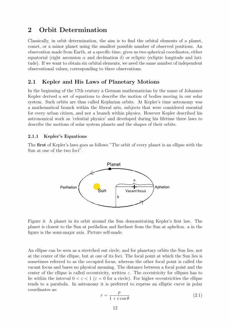
The first of Kepler’s laws goes as follows ”The orbit of every planet is an ellipse with theSun at one of the two foci”.

Figure 4: A planet in its orbit around the Sun demonstrating Kepler’s first law. Theplanet is closest to the Sun at perihelion and furthest from the Sun at aphelion. a in thefigure is the semi-major axis. Picture self-made.

An ellipse can be seen as a stretched out circle, and for planetary orbits the Sun lies, notat the center of the ellipse, but at one of its foci. The focal point at which the Sun lies issometimes referred to as the occupied focus, whereas the other focal point is called thevacant focus and bares no physical meaning. The distance between a focal point and thecenter of the ellipse is called eccentricity, written ε. The eccentricity for ellipses has tolie within the interval 0 < ε < 1 (ε = 0 for a circle). For higher eccentricities the ellipsetends to a parabola. In astronomy it is preferred to express an elliptic curve in polarcoordinates as:

r =p

1 + e cos θ(2.1)

12

where p is the semi-latus rectum, and (r, θ) are the polar coordinates, r being the distancefrom the focus. For a planet moving in an orbit around the Sun, r is the distance fromthe planet to the Sun and θ is defined to be the angle that runs from the current positionof the planet to the point at which the planet is closest to the Sun. The distance is thesmallest at perihelion, where θ = 0, and is the largest at aphelion, θ = 90. We canwrite this as two equations,

rmin =p

1 + e, rmax =

p

1− e (2.2)

The semi-major axis of the ellipse is defined as the arithmetic mean between these two:

a =rmin + rmax

2=

p

1− e2(2.3)

Similarly, the semi-minor axis is defined by the geometric mean between rmin and rmax:

b =√rminrmax =

p√1− e2

(2.4)

The semi-latus rectum p in these equations is defined as the harmonic mean between thetwo distances:

1

rmin− 1

p=

1

p− 1

rmax(2.5)

giving the following relation:pa = rminrmax = b2 (2.6)

and the eccentricity is defined as the coefficient of variation between rmin and rmax:

e =rmax − rminrmax + rmin

(2.7)

Finally, the area of the ellipse is defined as,

A = πab (2.8)

where for a circle (e = 0), r = p = rmin = rmax = a = b giving the area A = πr2.

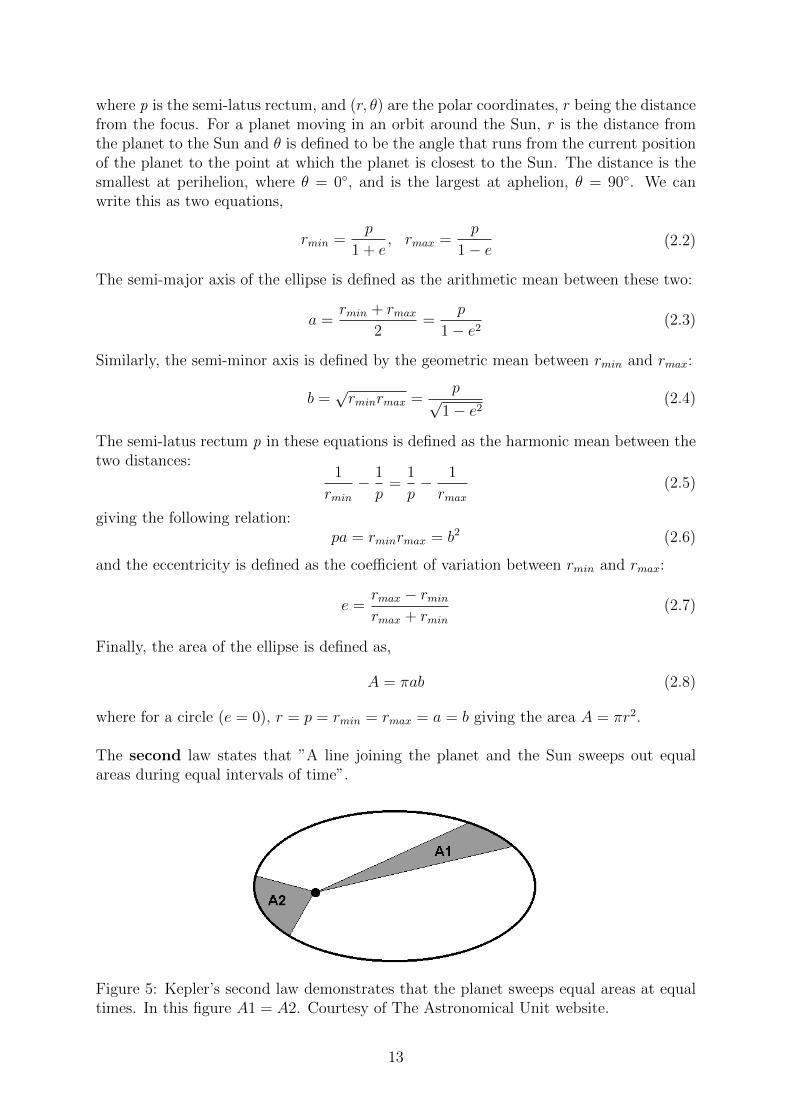
The second law states that ”A line joining the planet and the Sun sweeps out equalareas during equal intervals of time”.

Figure 5: Kepler’s second law demonstrates that the planet sweeps equal areas at equaltimes. In this figure A1 = A2. Courtesy of The Astronomical Unit website.

13

During a small time interval dt a planet moving in an elliptical orbit will sweep out asmall triangle with baseline r and hight rdθ. The area of this small triangle will then be:

dA =1

2· r · rdθ (2.9)

The areal velocity, that is the rate at which the area is swept out by the planet, is thus:

dA

dt=

1

2r2dθ

dt(2.10)

Since the planet moves in an elliptical orbit around the Sun, the distance r from theplanet to the Sun varies along the orbit. From equation (2.10) we see that the planetthen has to move faster when it is closer to the Sun, in order to sweep equal areas atequal times.

From equation (2.8) we know that the area of an elliptical orbit is A = πab, and theperiod of the orbit must therefore satisfy,

πab = P · 1

2r2θ (2.11)

where θ = dθ/dt.

The third of Kepler’s laws says that ”The square of the orbital period of a planet isproportional to the cube of the semi-major axis of its orbit”.

According to the third law by Kepler we have the following relationship:

P 2 ∝ a3 (2.12)

where P is the orbital period and a is the semi-major axis. Since this relationship shouldbe valid for each planet in our solar system we may write:

P 2planet

a3planet

=P 2Earth

a3Earth

= 1yr2

AU3(2.13)

which is the constant of proportionality, for a sidereal year (yr) and astronomical unit(AU).

In the case of a circular orbit, where the semi-major axis is equal to the radius of theorbit, this law is written as,

P 2 =4π2

GMR3 (2.14)

where P is the period, G is the gravitational constant, M is the mass of the most massivebody, and R is the radius, that is distance between the two centers of mass.

In practise, the rotation is about the barycenter of the two bodies, neither one with itscenter of mass exactly at one focus of an ellipse. However, the two orbits are both ellipsesand share a common focus at the barycenter. For a large mass ratio between the twoobjects, the barycenter may lie inside the more massive object, [Wikipedia, 2014].

14

2.2 Determining an Orbit from Two Position Vectors

In general, when describing the orbit for a planet or a comet, the orbital elements areused, since they give a quite clear understanding of the individual values. However, formodern orbit determination we use another method, depending on our knowledge of theposition and velocity of the object in question, at a specific instant. An alternative is touse, at least, two different positions on the orbit and the corresponding times. For thissecond technique of determining an orbit, the Gauss’s method is employed. Using thismethod the orbit may be described by two known position vectors ra and rb at times taand tb, in order to calculate the orbital elements.

The most difficult part of determining an orbit is the intermediate step of calculatingthe sector-triangle. I am presenting here a description of how this is done, where I havefollowed the method described in the Astronomy on the Personal Computer 4th ed., byO. Montenbruck and T. Pfleger, 2000, [Montenbruck and Pfleger, 2000].

2.2.1 The Sector-Triangle Ratio

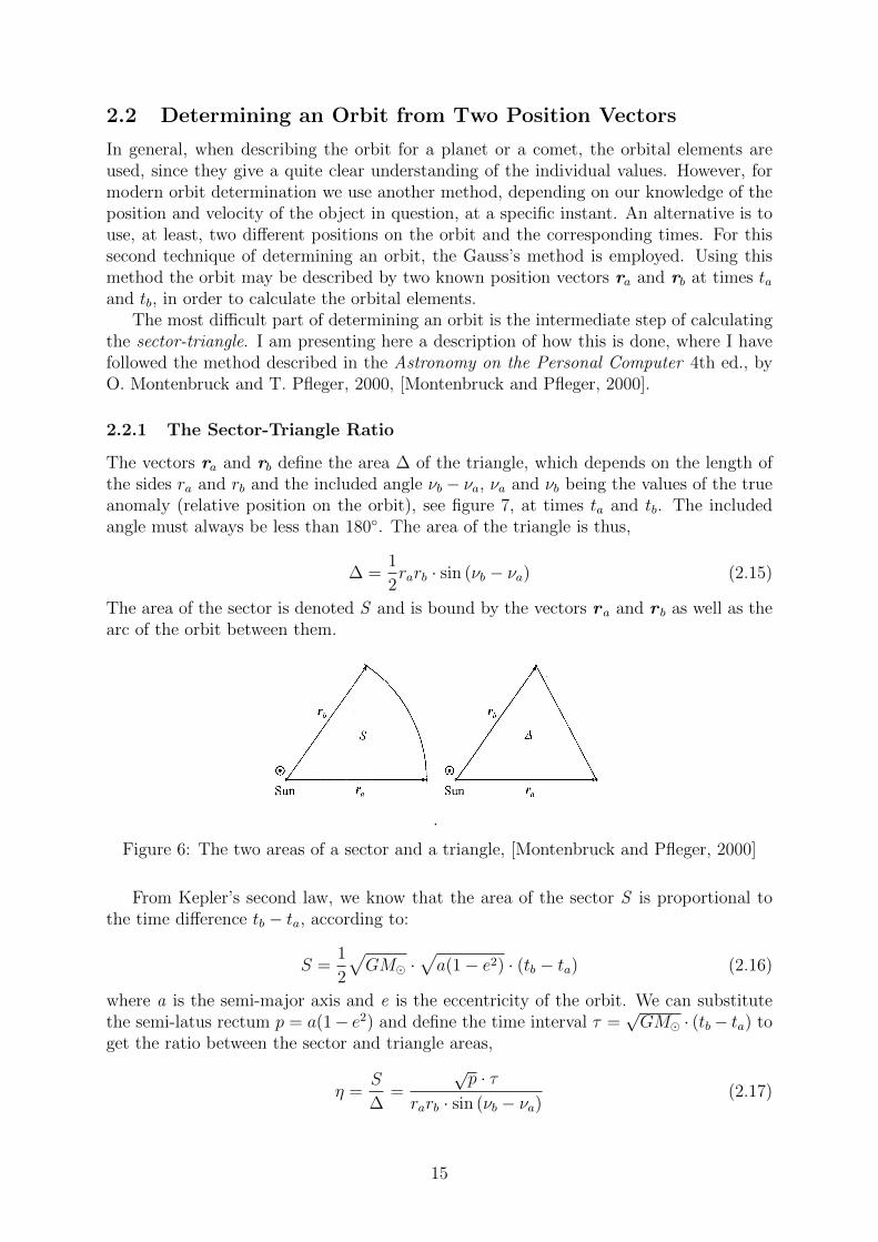
The vectors ra and rb define the area ∆ of the triangle, which depends on the length ofthe sides ra and rb and the included angle νb − νa, νa and νb being the values of the trueanomaly (relative position on the orbit), see figure 7, at times ta and tb. The includedangle must always be less than 180. The area of the triangle is thus,

∆ =1

2rarb · sin (νb − νa) (2.15)

The area of the sector is denoted S and is bound by the vectors ra and r b as well as thearc of the orbit between them.

.

Figure 6: The two areas of a sector and a triangle, [Montenbruck and Pfleger, 2000]

From Kepler’s second law, we know that the area of the sector S is proportional tothe time difference tb − ta, according to:

S =1

2

√GM ·

√a(1− e2) · (tb − ta) (2.16)

where a is the semi-major axis and e is the eccentricity of the orbit. We can substitutethe semi-latus rectum p = a(1− e2) and define the time interval τ =

√GM · (tb− ta) to

get the ratio between the sector and triangle areas,

η =S

∆=

√p · τ

rarb · sin (νb − νa)(2.17)

15

In trying to eliminate the semi-latus rectum p the equations for the two-body problemare utilized. Thence, we cannot write η as a solvable algebraic equation and must applythe following transcendental equation,

η = 1 +m

η2·W (

m

η2− l) (2.18)

where,

m =τ 2√

2(rarb + ra · r b)3

l =ra + rb

2√

2(rarb + ra · r b)− 1

2

(2.19)

and,

W (w) =

2g − sin (2g)

sin3 (g), g = 2 arcsin

√w 0 < w < 1

4

3+

4 · 63 · 5

w +4 · 6 · 83 · 5 · 7

w2 + ... w ≈ 0

sinh (2g)− 2g

sinh3 (g), g = 2 arsinh

√−w w < 0

(2.20)

2.3 Orbital Elements

The orbit of a celestial body is restricted to a plane that is determined by the Sun andtwo points ra and rb through which it passes. The unit vectors, both lying in the orbitalplane, are defined as,

ea =ra|ra|

e0 =r0|r0|

(2.21)

where r0 = rb − (rb · ea)ea. Taking the cross product of the two vectors we get theGaussian vector R, perpendicular to the orbital plane and normalized to unit length. Ris directed to the ecliptic longitude l = Ω − 90and latitude b = 90 − i, where Ω is theso called ascending node and i is the inclination. The Gaussian vector R is defined as:

R =

RX

RY

RZ

=

+ cos (90 − i) cos (Ω− 90)+ cos (90 − i) sin (Ω− 90)

+ sin (90 − i)

=

+ sin i sin Ω− sin i cos Ω

+ cos i

The ascending node and the inclination can thus be expressed in terms of the componentsof the vector R as follows,

Ω = 90 + arctan (Ry

Rx

) = arctan (−Rx

Ry

) (2.22)

i = 90 − arcsin (Rz) (2.23)

In order to calculate the other orbital elements we need the sector-triangle ratio, whichis described in the previous section. From this we get the semi-latus rectum p = (2·∆·η

τ)2

in terms of the triangle area ∆,

16

∆ =1

2rarb · sin(νb − νa) =

1

2rar0 (2.24)

Here ra and r b are the two vectors defining the area. To determine the eccentricity e,

Figure 7: The image shows the orbital elements of a planet. The same parameters areused for any solar system object, including minor planets and comets. Ω is the longitudeof the ascending node, ω is the argument of perihelion, where π = Ω +ω, Ω and ω actingin different planes, is the longitude of perihelion. ν is the true anomaly, and i is theinclination of the planetary orbit to the ecliptic. Courtesy of A. Roberge, John HopkinsUniversity, First Year Seminar Paper, May 5, 1997.

i.e. the shape, of the orbit we use the equation for the conic section,

r =p

1 + e · cos ν(2.25)

where we solve for e cos ν.

The eccentricity may be expressed in terms of the true anomaly at time ta: νa =arctan ( e·sin (νa)

e·cos (νa)) giving,

e =√

(e · cos (νa))2 + (e · sin (νa))2 (2.26)

Now that we know both the semi-latus rectum and the eccentricity, we can determine thesemi-major axis and the perihelion distance,

a =p

1− e2(2.27)

q =p

1 + e(2.28)

From the distance between the argument of latitude and the true anomaly, we get thelongitude of perihelion as well as the argument of perihelion,

π = ua − νa + Ω (2.29)

ω = ua − νa (2.30)

17

The last orbital element to be determined is the time of perihelion passage or the peri-helion date, which is defined as when the object passes closest to the Sun. This we can

calculate if we know the orbital period T = 2π√

a3

GM⊙ and the mean anomaly Ma and is

given by,

tp = ta −Ma√GM⊙a3

(2.31)

where the mean anomaly is obtained from Kepler’s equation:

Ma = Ea − e · sinEa (2.32)

In this equation Ea is the eccentric anomaly.We have now defined all the parameters which determine the orbit of a solar system

object.

2.4 Methods for Determining the Orbit

There are various methods for determining the orbit of a comet, what will be mentionedhere is the so called Gauss method.

2.4.1 The Shortened Gauss Method

The distance from the comet to Earth is written ρ, and the geocentric position of thecomet is thus given by,

ρe = R + r (2.33)

where r is the comet’s position relative to the Sun, R is the geocentric position of theSun, and e is a unit vector directed towards the comet from Earth. In order to determinethe orbit of a comet at least three observations e1, e2, e3 must be available. In additionwe assume that the coordinates of the Sun R1, R2 and R3 at the times of observationt1 < t2 < t3 are known. From these data we want to try to calculate the distances ρ1, ρ2

and ρ3 at these different times. When we know these we can determine the heliocentricpositions, and thus get the orbital elements. All the points lie in a single plane alongwith the Sun, for an unperturbed Keplerian motion. This allows us to write one positionvector as a combination of the other two, for example,

r 2 = n1r 1 + n3r 3 (2.34)

This is the fundamental equation of the Gauss method and is called the equation of theorbital plane. The factors n1 and n3 can be expressed in terms of the areas of the triangles,figure 8, bounded by the vectors r 1, r 2, and r 3, that is,

n1 =∆1

∆2

n3 =∆3

∆2

(2.35)

For small arcs of the orbit we can replace the triangle areas with the corresponding sectorareas, which are proportional to the time intervals τi. The factors can thus be written as,

n1 ≈τ1

τ2

n3 ≈τ3

τ2(2.36)

18

Now that we know approximate values for n1 and n3 we can calculate the geocentricdistances using the following three equations:

ρ1 =1

n1D(n1D11 −D12 + n3D13)

ρ2 =1

−D(n1D21 −D22 + n3D23)

ρ3 =1

n3D(n1D31 −D32 + n3D33)

(2.37)

Here D = e1 · d 1 = e2 · d 2 = e3 · d 3 and Dij = d i ·Rj, where the vectors di are definedas d1 = e2 × e3, d2 = e3 × e1, and d3 = e1 × e2.

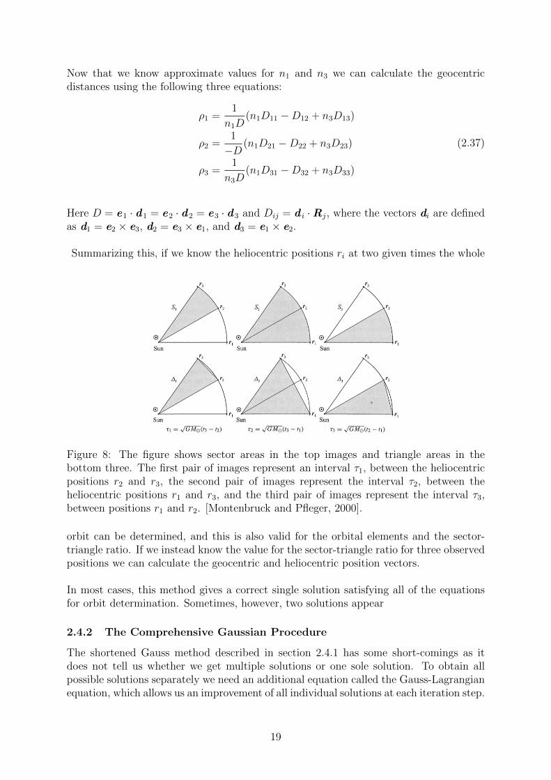
Summarizing this, if we know the heliocentric positions ri at two given times the whole

Figure 8: The figure shows sector areas in the top images and triangle areas in thebottom three. The first pair of images represent an interval τ1, between the heliocentricpositions r2 and r3, the second pair of images represent the interval τ2, between theheliocentric positions r1 and r3, and the third pair of images represent the interval τ3,between positions r1 and r2. [Montenbruck and Pfleger, 2000].

orbit can be determined, and this is also valid for the orbital elements and the sector-triangle ratio. If we instead know the value for the sector-triangle ratio for three observedpositions we can calculate the geocentric and heliocentric position vectors.

In most cases, this method gives a correct single solution satisfying all of the equationsfor orbit determination. Sometimes, however, two solutions appear

2.4.2 The Comprehensive Gaussian Procedure

The shortened Gauss method described in section 2.4.1 has some short-comings as itdoes not tell us whether we get multiple solutions or one sole solution. To obtain allpossible solutions separately we need an additional equation called the Gauss-Lagrangianequation, which allows us an improvement of all individual solutions at each iteration step.

19

The Gauss-Lagrangian equation is derived from improved approximations of the triangle-area ratios. These were formulated by Johann Franz Encke, one of Gauss’s students, andlook like the following,

n1 =τ1

τ2

+1

6τ1τ3(1 +

τ1

τ2

) · 1

r32

n3 =τ3

τ2

+1

6τ1τ3(1 +

τ3

τ2

) · 1

r32

(2.38)

However, we still do not know the distance r2. Inserting equation 2.38 along with thefollowing expressions,

ρ0 = − 1

D(n10D21 −D22 + n30D23) σ = +

1

D(µ1D21 + µ3D23) (2.39)

wheren10 =

τ1

τ2

n30 =τ3

τ2

µ1 =1

6τ1τ3(1 +

τ1

τ2

) µ3 =1

6τ1τ3(1 +

τ3

τ2

)(2.40)

into the relation for the geocentric distance ρ2 in equation 2.37 we get,

ρ2 = ρ0 −σ

r32

(2.41)

from which r2 can be derived.However, from equation 2.33 we get the following relation for r2,

r 2 = ρ2e2 −R2

representing the Sun-Earth-Planet triangle, from which we get the relationship,

r2 =√

(ρ2 − γR22)2 +R2

2(1− γ2) (2.42)

where γ = e2 · R2

R2.

Combining the two relations for the heliocentric distance r2 we get the so calledGauss-Lagrangian equation,

3

√σ

ρ0 − ρ2

=√

(ρ2 − γR22)2 +R2

2(1− γ2) (2.43)

From this we can determine the unknowns ρ2 and r2. When we know r2, the triangle-arearatios n1 and n3 can be calculated and thus also the geocentric distances ρ1 and ρ3, andtogether with ρ2 we can also calculate our heliocentric position vectors r 1,2,3.

Doing so for each (ρi, ri) pair we end up with, at most, three different orbits which cor-respond to the different observations. Now, when solving this Gauss-Lagrangian equationwe need to find the intersection of the two equation,

r(ρ) = 3

√σ

ρ0 − rhor(ρ) =

√(ρ− γR2)2 +R2(1− γ2) (2.44)

20

where, for small parts of an orbit, σ ≈ ρ0R3.

In the Gauss program a function called SolveGL is used for the computation of the Gauss-Lagrangian equation, giving up to three solutions, that is three different values for ρ. Thenegative solutions, however, are eliminated since they have no physical reality.

Due to Encke’s approximations, the Gauss-Lagrangian equation doesn’t provide exactsolutions of the orbit determination problem. If we, on the other hand, use these ap-proximations along with the iteration of the triangle-area ratios in the shortened Gaussmethod, we obtain a much better result.

So, for the comprehensive Gaussian orbit determination method we use three observa-tions (e1, e2, e3), along with the Sun’s corresponding geocentric coordinates (R1, R2,R3), and time intervals (τ1, τ2, τ3). To correct for the triangle-area ratios, the last twoequations in equation 2.40 are used as initial an approximation. The next step is tocalculate ρ0 and σ and, for these values solve the Gauss-Lagrangian equation. From thiswe get three possible solutions for the geocentric distance ρ2, where the first solutionis chosen in order to calculate the heliocentric distance r2. The triangle-area ratios inequation 2.38 are thereafter calculated along with the geocentric distances in equation2.37. Using equation 2.33 we get the corresponding heliocentric position vectors.

As an initial estimate for the correction terms for the trianle-area ratios, µ1 = (τ1τ3/6)(1+τ1/τ2) and µ3 = (τ1τ3/6)(1 + τ3/τ2) are used.

In order to solve the Gauss-Lagrangian equation, the values of ρ0 and σ are firstcalculated. From solving the equation the first of three obtained solutions for ρ2 ischosen. Once our ρ2 is known we can calculate the corresponding heliocentric distancer2.

The triangle-area ratios are calculated using equation 2.38 and using 2.37 also thegeocentric distances (ρ1, ρ2, ρ3).

From equation 2.33 the heliocentric position vectors (r1, r2, r3) can now be calculated.For every two heliocentric position vectors and corresponding interval τ , the sector-

triangle ratios (η1, η2, η3) are calculated using equation (2.18).Improved values for µ1 and µ3 can now be acquired for the correction terms for the

triangle-area ratios.

This procedure is repeated until no significant changes appear in µ1, µ3, as well as in therest of the values. When the values for µ1 and µ3 no longer show any significant changes,r1 and r3, along with τ2, can be used to calculate the orbital elements.

Should the Gauss-Lagrangian equation show more than one solution, the whole processhas to be repeated based on the second or third solution for ρ2. Here, it may be necessaryto consider the plausibility of some of the orbit solutions and eliminate the extreme values.In very doubtful cases, a fourth observation may be utilized in order to identify the correctorbit of the comet, from a set of multiple solutions.

21

3 Using the GAUSS Program to Obtain the Orbital

Elements

The orbital elements, which have been presented in section (2.3), can be attained using aprogram written in C++ called the GAUSS program, [Montenbruck and Pfleger, 2000].The program is based on the comprehensive Gaussian method described in section 2.4.2,and requires values for right ascension and declination from three observations to de-termine an orbit. These coordinates are put into the program on three lines, followedby the equinox related to the observed positions and the equinox that is wanted for thespecification of the achieved orbital elements.

These elements are calculated in the ecliptic coordinate system, since they shouldalways be relative to the ecliptic. The equinox can therefore be chosen independently.

3.1 Results from the GAUSS program

For this project I have been using data, taken from the Minor Planets Center website, fortwo comets; C/2011 L4 PANSTARRS and C/2012 S1 ISON, to try to find their respectiveorbital elements. The reason I chose these particular targets is that they were passingclose to the Sun and were therefore of great interest during the time of my project. TheGAUSS program does not, however, take into account the ephemerides of the solar systemplanets. Since a massive planet like Jupiter might have a noticeable impact on the orbitof a comet, the results obtained from running the program are not always correct. Istarted off by using known equatorial coordinates for comet C/2011 L4 PANSTARRS. Aset of three data points, containing the knowledge of the date on which they were taken,along with the comet’s right ascension (RA), in units (h,m,s) and declination (in units(,’,”), are inserted into the program. Using the comprehensive Gaussian procedure, asexplained above, the program first transforms the inserted equatorial coordinates intoecliptic coordinates, and thereafter gives the orbital elements of the chosen comet. Iinitially made the assumption that the accuracy of the results would depend on theseparation of the chosen dates, where the result would be poor for dates very closetogether and better for dates that were more spread. To test this I am using both closedates as well as more spread ones. To be able to see the accuracy in my results, and ifmy hypothesis was correct, I’ve looked at data from the Minor Planet Center website,in order to compare the orbital elements stated there with the ones I obtained using theGAUSS program, and from this make some conclusions.

C/2011 L4 PANSTARRS

For comparison and determination of the validity of the results obtained from runningthe program with different input data, orbital element data from the IAU Minor PlanetCenter website is also included. The data found online for C/2011 L4 PANSTARRS are:

22

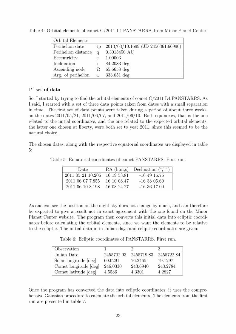
Table 4: Orbital elements of comet C/2011 L4 PANSTARRS, from Minor Planet Center.

Orbital ElementsPerihelion date tp 2013/03/10.1699 (JD 2456361.66990)Perihelion distance q 0.3015450 AUEccentricity e 1.00003Inclination i 84.2083 degAscending node Ω 65.6658 degArg. of perihelion ω 333.651 deg

1st set of data

So, I started by trying to find the orbital elements of comet C/2011 L4 PANSTARRS. AsI said, I started with a set of three data points taken from dates with a small separationin time. The first set of data points were taken during a period of about three weeks,on the dates 2011/05/21, 2011/06/07, and 2011/06/10. Both equinoxes, that is the onerelated to the initial coordinates, and the one related to the expected orbital elements,the latter one chosen at liberty, were both set to year 2011, since this seemed to be thenatural choice.

The chosen dates, along with the respective equatorial coordinates are displayed in table5:

Table 5: Equatorial coordinates of comet PANSTARRS. First run.

Date RA (h,m,s) Declination (,’,”)2011 05 21 10.206 16 19 53.81 -16 49 16.762011 06 07 7.855 16 10 08.47 -16 38 05.602011 06 10 8.198 16 08 24.27 -16 36 17.00

As one can see the position on the night sky does not change by much, and can thereforebe expected to give a result not in exact agreement with the one found on the MinorPlanet Center website. The program then converts this initial data into ecliptic coordi-nates before calculating the orbital elements, since we want the elements to be relativeto the ecliptic. The initial data in in Julian days and ecliptic coordinates are given:

Table 6: Ecliptic coordinates of PANSTARRS. First run.

Observation 1 2 3Julian Date 2455702.93 2455719.83 2455722.84Solar longitude [deg] 60.0291 76.2465 79.1297Comet longitude [deg] 246.0330 243.6940 243.2784Comet latitude [deg] 4.5586 4.3301 4.2827

Once the program has converted the data into ecliptic coordinates, it uses the compre-hensive Gaussian procedure to calculate the orbital elements. The elements from the firstrun are presented in table 7:

23

Table 7: Orbital elements of comet PANSTARRS. First run.

Orbital ElementsPerihelion date tp 2013/04/11.881 (JD 2456394.381)Perihelion distance q 0.407582 AUSemi-major axis a -41.669404 AUEccentricity e 1.009781Inclination i 111.0487 degAscending node Ω 63.7618 degLong. of perihelion π 32.7989 degArg. of perihelion ω 329.0371 deg

By comparing the numbers of this result to those of the orbital elements presented intable 4, all elements seem to agree rather well since they only differ by some unit digits,with an exception in inclination, which differs with more than that. This could tell usthat, at that point, the comet may not have passed close to any of the more massiveplanets, so that its orbit had not been perturbed.

2nd set of data

After the first run I proceeded by using a set of data points slightly less separated thanthe first ones. These data points were all taken in April of 2012, on three following days;2012/04/22, 2012/04/23, and 2012/04/24. The initial dates and equatorial coordinatesare presented in table 8:

Table 8: Equatorial coordinates of comet PANSTARRS. Second run.


In this table we can clearly see that the planet has not had time to make any significantchanges in position, so we can expect a poor result as an output for these initial data.Also these coordinates are converted onto an ecliptic reference frame, to be read by theprogram, the dates presented in Julian days:

Table 9: Ecliptic coordinates of PANSTARRS. Second run.

Observation 1 2 3Julian Date 2456039.79 2456040.75 2456042.18Solar longitude [deg] 32.5535 33.4843 34.8826Comet longitude [deg] 253.7319 253.5838 253.3531Comet latitude [deg] -2.8905 -2.9358 -3.0054

As the program was run using this set of data are presented, I got the following valuesfor the orbital elements:

24

Table 10: Orbital elements of comet PANSTARRS. Second run.


As we see when comparing to the orbital elements from the Minor Planet Center in table4, it is quite clear that the results from this run are in very bad agreement with those.The reason that comes to mind for this is the selection of such close dates, since to get astatistically good value it is favorable to select separated values.

3rd set of data

I then moved on to using coordinates from later the same year (2012), but with somemore separation in time, compared to the previous two runs. The dates I used here are;2012/07/23, 2012/08/21, and 2012/10/01. The initial equatorial coordinates were:

Table 11: Equatorial coordinates of comet PANSTARRS. Third run.


We see here that the change in position is a bit more than in the previous run, and cantherefore expect slightly better values this time. The data in ecliptic coordinates are asfollows:

Table 12: Ecliptic coordinates of PANSTARRS. Third run.

Observation 1 2 3Julian Date 2456132.40 2456160.61 2456201.50Solar longitude [deg] 121.4105 148.4429 188.2126Comet longitude [deg] 231.8871 229.6928 232.8041Comet latitude [deg] -7.0313 -7.7452 -8.8809

Using these coordinates in the program I got the following values for the orbital elementsof the comet PANSTARRS:

25

Table 13: Orbital elements of comet PANSTARRS. Third run.

Orbital ElementsPerihelion date tp 2013/03/10.269 (JD 2456361.769)Perihelion distance q 0.299959 AUSemi-major axis a 182.822052 AUEccentricity e 0.998359Inclination i 85.0523 degAscending node Ω 65.8012 degLong. of perihelion π 39.6705 degArg. of perihelion ω 333.8693 deg

We see here that, compared to the pervious run, the orbital elements are a lot closer tothose from the Minor Planet Center, in table 4, which is likely to be due to the largerseparation of dates.

4th set of data

Next, I was using positions taken during the first half of 2013. The separation of theseis about the same as in the previous set. The equatorial coordinates for the dates2013/03/31, 2013/04/28, and 2013/05/07 are:

Table 14: Equatorial coordinates of comet PANSTARRS. Fourth run.

Date RA (h,m,s) Declination (,’,”)2013 03 31 3.9390 00 31 40.04 35 27 40.62013 04 28 21.483 00 13 58.40 65 22 23.02013 05 07 1.8430 00 00 10.83 72 18 39.1

We now see, compared to the previous runs, that the comet has changed its positionsignificantly, with emphasis on the declination. When the program transformed theseinitial equatorial coordinates into ecliptic coordinates the following output was obtained:

Table 15: Ecliptic coordinates of PANSTARRS. Fourth run.


We I ran the program with this set of initial data I got two solutions for the orbitalelements of the comet. The first solution is:

26

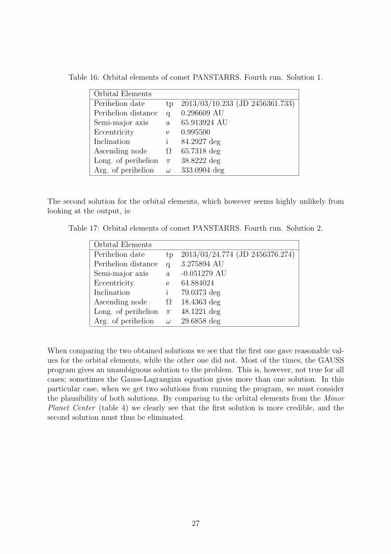
Table 16: Orbital elements of comet PANSTARRS. Fourth run. Solution 1.


The second solution for the orbital elements, which however seems highly unlikely fromlooking at the output, is:

Table 17: Orbital elements of comet PANSTARRS. Fourth run. Solution 2.


When comparing the two obtained solutions we see that the first one gave reasonable val-ues for the orbital elements, while the other one did not. Most of the times, the GAUSSprogram gives an unambiguous solution to the problem. This is, however, not true for allcases; sometimes the Gauss-Lagrangian equation gives more than one solution. In thisparticular case, when we get two solutions from running the program, we must considerthe plausibility of both solutions. By comparing to the orbital elements from the MinorPlanet Center (table 4) we clearly see that the first solution is more credible, and thesecond solution must thus be eliminated.

27

C/2012 S1 ISON

From here I moved on to inserting data from another comet, C/2012 S1 ISON, into theGAUSS program, to get its orbital elements. Also here, I compared my output data tothe one found on the Minor Planet Center website, to check its validity. Because of themore recent discovery of this comet, as compared to the one from PANSTARRS, lessdata was available on the Minor Planet Center. I therefore considered it sufficient to usethree sets of initial data for this comet, starting from data taken with a small separationin time, and moving on to more separated dates. By doing so, I could test if my initialhypothesis was correct.

Also for comet ISON, I have included data from the IAU Minor Planet Center website,for comparison with the data I obtained from the GAUSS program. The orbital elementsfor this comet found there are the following:

Table 18: Orbital elements for comet C/2012 S1 ISON, from Minor Planet Center.

Orbital ElementsPerihelion date tp 2013/11/28.87041Perihelion distance q 0.0124527 AUEccentricity e 1.0000Inclination i 62.36426 degAscending node Ω 295.65952 degArg. of perihelion ω 345.56137 deg

1st set of data

The first set of equatorial coordinates that I used for comet C/2012 S1 ISON were takenon three following days, in September 2012; 2012/09/21, 2012/09/22, and 2012/09/23.These coordinates are presented in table 19:

Table 19: Equatorial coordinates of comet ISON. First run.

Date RA (h,m,s) Declination (,’,”)2012 09 21 19.156 08 12 51.77 +27 50 13.42012 09 22 04.211 08 13 09.15 +27 49 56.92012 09 23 10.434 08 13 37.82 +27 49 32.4

During this small period of time the comet has not moved very much, so the result wemay expect is not in quite accordance with the comparison values in table 18. The initialcoordinates in ecliptic coordinates are as follows:

28

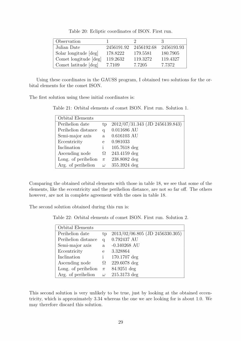
Table 20: Ecliptic coordinates of ISON. First run.


Using these coordinates in the GAUSS program, I obtained two solutions for the or-bital elements for the comet ISON.

The first solution using these initial coordinates is:

Table 21: Orbital elements of comet ISON. First run. Solution 1.


Comparing the obtained orbital elements with those in table 18, we see that some of theelements, like the eccentricity and the perihelion distance, are not so far off. The othershowever, are not in complete agreement with the ones in table 18.

The second solution obtained during this run is:

Table 22: Orbital elements of comet ISON. First run. Solution 2.


This second solution is very unlikely to be true, just by looking at the obtained eccen-tricity, which is approximately 3.34 whereas the one we are looking for is about 1.0. Wemay therefore discard this solution.

29

2nd set of data

Next I used initial values where the first two were a bit more separated in time. The datathis time were taken on the following days: 2012/01/28, 2012/09/22, and 2012/09/23.The equatorial coordinates for the comet on these dates were:

Table 23: Equatorial coordinates of comet ISON. Second run.


Due to the bigger separation of the two first dates we may expect better values of theorbital elements. These initial coordinates transformed into ecliptic coordinates are:

Table 24: Ecliptic coordinates of ISON. Second run.


The orbital elements I obtained from this second set of position data for comet ISON arethe following:

Table 25: Orbital elements of comet ISON. Second run.

Orbital ElementsPerihelion date tp 2013/05/02.710 (JD 2456415.210)Perihelion distance q [AU] 0.437822Semi-major axis a [AU] -0.905001Eccentricity e 1.483781Inclination i 167.4451 degAscending node Ω 248.5172 degLong. of perihelion π 148.9737 degArg. of perihelion ω 260.4565 deg

In contrast to what I predicted, these values are in slightly less agreement with those intable 18, in spite of the larger separation in time between the two first data points. It’sdifficult to say exactly what may have caused such bad values. One explanation might bethe influence of a planet’s gravitational pull, causing perturbations of the orbit. Anothermight be due to a bad initial guess made by the program, based on the initial observations,since the separation between the second and third date is very small compared to theseparation between the first two dates. Because of this the fitting mainly considers twodata points leading to a poor approximation of the orbit. The eccentricity obtained here,

30

in any case, seems to be that of a hyperbola, whereas the one in table 18 is that of aparabolic orbit, so the conclusion that can be made is that this is not a good solution.

Figure 9: C/2012 S1 ISON, Jan 28, 2012. Image taken from NASA; JPL Small-BodyDatabase Browser.

Figure 10: C/2012 S1 ISON, Sep 22, 2012. Image taken from NASA; JPL Small-BodyDatabase Browser.

Since the comet does not pass very close to Jupiter, as seen in figures 9 and 10, theperturbations might not be so much due to the gravitational pull of the planet, but causedby other parameters, most likely within the program itself.

3rd set of data

The third and last run I did, using positional data from comet ISON, I used coordinatesfrom the following dates: 2012/09/23, 2012/09/21, and 2011/12/28. Due to the smallrange of data available for comet ISON when I did this project, these were the mostseparated dates I could find, giving the following equatorial coordinates:

Table 26: Equatorial coordinates of comet ISON. Third run.


Since these positions are slightly more separated than the previous ones I expected abetter result for the orbital elements of the comet. These positions in ecliptic coordinates

31

Table 27: Ecliptic coordinates of ISON. Third run.


are:

Finally, the orbital elements I achieved when running the GAUSS program with theseinitial positions are the following:

Table 28: Orbital elements of comet ISON. Third run.


As expected, these orbital elements much closer to those from the Minor Planet Center(table 18), with some exceptions in perihelion date and inclination. The most obviousreason for the improved results is the bigger separation in time for the chosen coordinates.

32

4 Concluding remarks

From the results obtained using the FOTO program to get the equatorial coordinates ofa comet, we learn that it is necessary to know the coordinates of at least three referencestars. A way to explore this program more would be to use a variety of reference stars,for different comets. But, for the purpose of showing its stability for a different numberof reference stars, the example included in this thesis is sufficient.

The GAUSS program gives fairly accurate values of the orbital elements. There are,however, some disadvantages to the program. First of all, it is programmed to take onlythree initial observations, so the accuracy cannot really be increased. Secondly, it doesnot include the planets’ ephemerides, which may cause perturbation on the orbit if thecomet passes within a planet’s gravitational field. Measuring after the comet has passedclose to a planet may give bad values. Thirdly, the program makes an initial guess basedon the chosen observations, and depending on the quality of this guess the quality ofthe output values vary. The program does not give formal errors of the obtained orbitalelements either, which makes it hard to estimate the precision of the different solutions.

In order to get better solutions it would be favorable to add more than three initialobservations to the program. This would mean that the code be rewritten, to take morethan three observations. Another suggestion is using a program which is already pro-grammed to take more than three observations, and which gives the user the option toinclude the planetary ephemerides. It would also be easier to determine the accuracy ofan obtained solution, if the formal errors were given along with it.

Overall, the GAUSS program, presented in [Montenbruck and Pfleger, 2000], gives afairly good solution to the orbital elements, but is, somewhat based on luck when itcomes to choosing initial observations. Some of the solutions did, however, give veryaccurate values of the orbital elements of the two comets, at times, showing that theprogram can be quite sufficient for orbit determination of solar system objects. I havelearned a lot from this project, not only about astrometry as a field of research, but alsohow to obtain the equatorial coordinates of a solar system object, in this case a comet,and from there calculate its orbital elements. From observing the motions of comets,one may get a deeper knowledge of the physical characteristics of these objects, and thuslearn a bit more about our universe as a whole.

33

References

[CSIRO Australia, 2004] CSIRO Australia (2004). Brief history of astrometry.

[Festou et al., 1993] Festou, M., H., R., and R.M., W. (1993). History on comets - i.Astronomy and Astrophysics Reviews, 4:363–447.

[Marsden, 1977] Marsden, B. (1977). Carl friedrich gauss, astronomer. Journal of theRoyal Astronomical Society of Canada, 71:309–322.

[Montenbruck and Pfleger, 2000] Montenbruck, O. and Pfleger, T. (2000). Astronomy onthe Personal Computer.

[Perryman, 2012] Perryman, M. (2012). The history of astrometry. arXiv:1209.3563v1[physics.hist-ph].

[Tapley et al., 2004] Tapley, B., Schutz, B., and Born, G. (2004). Statistical Orbit De-termination.

[University of Virginia, 2009] University of Virginia (2009). History of astrometric mea-surements in astronomy.

[Vaccari, 2000] Vaccari, M. (2000). B. the historical developement of astrometry.

[van Altena, 2013] van Altena, W. (2013). Astrometry for Astrophysics: Methods, Mod-els, and Applications.

[Wikipedia, 2014] Wikipedia (2014). Kepler’s laws of planetary motion — wikipedia, thefree encyclopedia.

34

A Images of Comet PANSTARRS

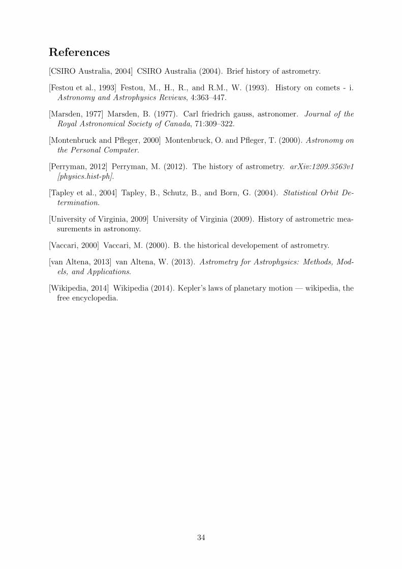
Figure 11: C/2011 L4 PANSTARRS, Nov 12, 2013. Image taken from NASA; JPLSmall-Body Database Browser.

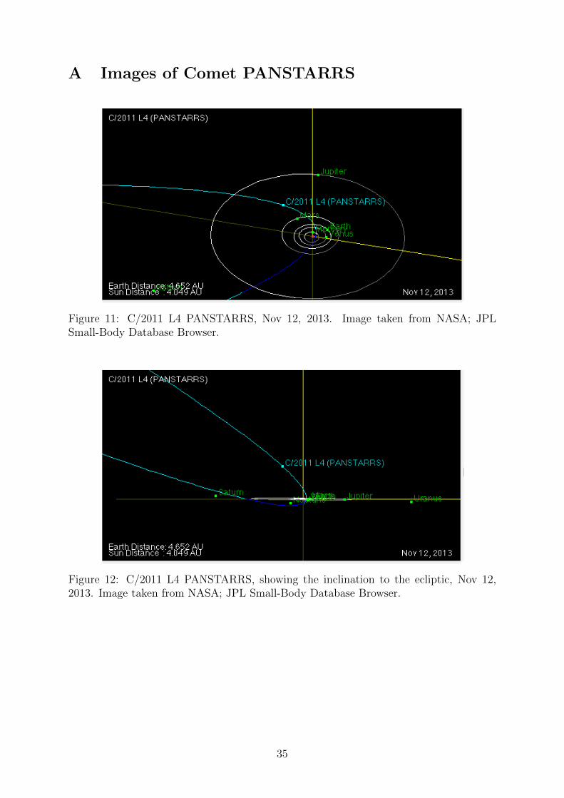
Figure 12: C/2011 L4 PANSTARRS, showing the inclination to the ecliptic, Nov 12,2013. Image taken from NASA; JPL Small-Body Database Browser.

35

B Images of Comet ISON

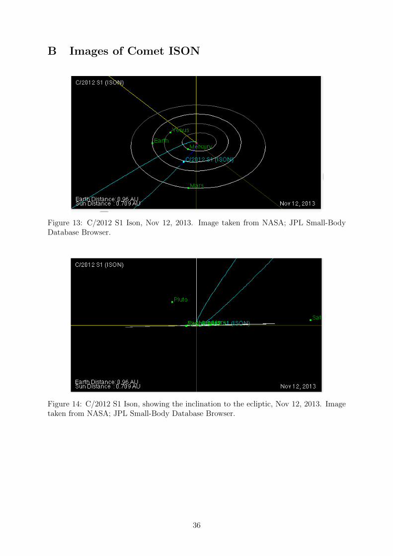
Figure 13: C/2012 S1 Ison, Nov 12, 2013. Image taken from NASA; JPL Small-BodyDatabase Browser.

Figure 14: C/2012 S1 Ison, showing the inclination to the ecliptic, Nov 12, 2013. Imagetaken from NASA; JPL Small-Body Database Browser.

36

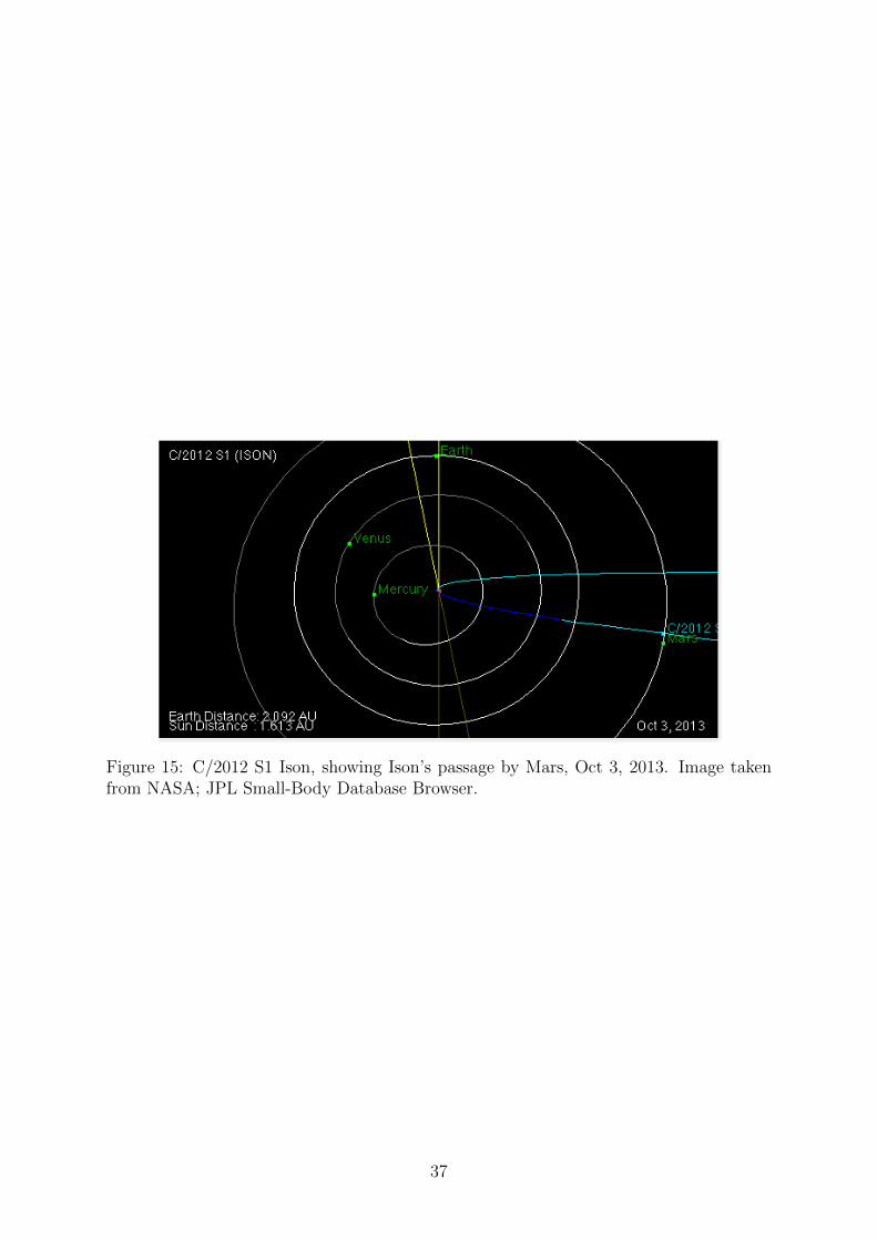
Figure 15: C/2012 S1 Ison, showing Ison’s passage by Mars, Oct 3, 2013. Image takenfrom NASA; JPL Small-Body Database Browser.

37

relative astrometry and orbit determination

Documents