1

Reliable Surface Extraction from Point-Clouds using Scanner-Dependent Parameters

Hiroshi Masuda1, Ichiro Tanaka2, and Masakazu Enomoto3

1The University of Tokyo, masuda@sys.t.u-tokyo.ac.jp

2Tokyo Denki University, tanaka@cck.dendai.ac.jp 3The University of Tokyo, eno@nakl.t.u-tokyo.ac.jp

ABSTRACT

Phase-based and time-of-flight laser scanners can be used to capture dense point-clouds of industrial plants. Our goal is to reconstruct 3D models of components in industrial plants. For robustly extracting surfaces, the standard deviation of residuals in surface fitting has large impact on the result. The standard deviation is one of basic parameters in the least-squares, robust estimate, region growing, and RANSAC. However, it is not easy to estimate the standard deviations of fitting errors in a wide range of field, because the standard deviations vary in a point-cloud, according to the sizes, distances, and materials of scanned objects. In this paper, we investigate the distributions of residuals in surface fitting using experimental data, and derive prediction functions of the standard deviations for measurement errors. Our experimental result shows that our prediction functions are effective for reliably extracting surfaces of diverse sizes, distances, and materials.

Keywords: point-cloud, surface extraction, as-built modeling, point processing. DOI: 10.3722/cadaps.2011.xxx-yyy

1 INTRODUCTION

Mid/long-range laser scanners have been widely used to measure large-scale environment mainly in the field of terrestrial surveying. Recently, these scanners are significantly improved in the quality and measurement speed, and they come into use in other fields for measuring factories, power plants, heavy goods, buildings, transportation infrastructure, and so on. Large facilities require repetitive maintenance and renovation in their long lifecycles. So, as-built 3D modeling based on point-clouds is very important in maintenance and asset management, because model-based simulation is effective for reducing the maintenance cost.

Two types of laser scanners are commonly used for surveying large-scale environment. One is the time-of-flight scanner, which measures the round-trip travel time of the laser pulses. This type of scanner can measure a wide range of field, but measurement speed is not very fast. The other type is the phase-based laser scanner, which radiates continuous modulated laser pulses and calculates distances using the phase difference between the emitted and received signals. The phase-based scanners cover only a mid-range of distance, but the measurement speed is ten times faster than the time-of-flight scanners.

We consider that the phase-based laser scanners are more suitable for acquiring point-clouds of industrial plants, because the mid-range is enough to cover the scales of most industrial plants, and quick scanning is very important for industrial plant surveys in order to avoid disturbing operations. While the maximum measurement distance of the early phase-based scanner is 57 meters, the ones of the latest phase-based scanners are more than 150 meters. Although there is no common definition of the mid-range scanners, we consider the mid-range as the distance approximately from 1 m to 30 m in this paper.

In this paper, we discuss surface extraction from point-clouds of industrial plants. When we extract surfaces from point-clouds, we often use segmentation and surface fitting techniques.

2

Segmentation techniques are used to find regions with continuous surfaces, of continuous curvatures, or of the same equations [1-5]. Surface fitting techniques are used determine the surface equations by using the least-squares method [6], the robust estimate [7-8], or the RANSAC method [9-10]. Segmentation and surface fitting are often used in a complementary manner [6].

In both segmentation and surface fitting, thresholds and weight values have large impact on the result. However, it is not easy to optimize these parameters in the case of reverse engineering for industrial plants. Compared to the case of mechanical parts, difficulty arises because of the diversity of sizes and distances of components included in industrial plants. In previous works, adaptive thresholds are calculated using point density [11-12] or principal component analysis [4-5] using neighbor points, but these methods do not always produce good estimates, when point-clouds are very noisy and the component sizes and distances are not uniform [13].

In surface extraction, the values of point spacing and the standard deviation of residuals are especially important; the point spacing is used for segmenting continuous regions, and the standard deviation of fitting errors is used for thresholds of RANSAC and region growing. If these values can be stably estimated, the reliability of surface fitting will be greatly improved.

In this paper, we discuss how point spacing and the standard deviation can be estimated using parameters that are dependent on measurement and scanners. We derive point spacing using measurement conditions, and derive the standard deviation based on experimental results.

In the following section, we will explain point-spacing and the standard deviations in surface extraction. In Section 3, we describe our experiments to derive properties of point-clouds and then we discuss how to estimate the standard deviation. In Section 4, we explain surface extraction, and finally we conclude in Section 5.

2 PARAMETERS FOR SURFACE EXTRACTION

The standard deviation of residuals and the point spacing play important roles in segmentation and surface fitting for point-clouds. In this Section, we discuss these parameters.

2.1 Estimation of Point Spacing for Segmentation

First, we consider generating mesh models by connecting neighbor points. In mid/long-range scanners, the directions of laser beams are controlled by the azimuth angle q and the zenith angle f , and coordinates are measured at regular angle intervals, as shown in Fig. 1. Therefore, mesh models can be easily generated by connecting adjacent points in the sequence of points along the azimuth and the zenith angles.

Polygons in a mesh model are generated only when the lengths of edges are less than a certain threshold. The threshold depends on the distance from the laser scanner. Fortunately, mid/long-range scanners output coordinates in the scanner-centered coordinate system, and we can calculate the distance from the scanner for point p as | |p . In addition, the angle spacing is constant during each scanning.

When the angle spacing φΔ is given and φ θΔ = Δ , we can estimate the point-spacing is of point

ip , as shown in Fig. 2:

2| || ( , ) |i

ii i

s φΔ=pp n

, (2.1)

where in is the normal vector at point ip , and the angle spacing φΔ is very small. The normal vector

can be estimated using neighbor points of ip [11, 14].

When the distance between two adjacent points are more than a certain threshold, the two points are regarded as ones on different surfaces. We define the threshold as ik s× , where k is a noise factor.

Fig 15 shows a segmentation result based on the threshold with 1 . 2k = .

3

(a) The azimuth angle and zenith angle. (b) Points at the regular angle intervals.

Fig. 1: Measurement by mid/long-range laser scanners.

Fig. 2: Estimation of point spacing.

2.2 Standard Deviation of Residuals in Surface Fitting

In surface fitting, coefficients of a surface equation are calculated by using point samples. The least-squares method is often used for surface fitting, but the least-squares method produces the maximum likelihood result only when the residuals follow the normal distribution and their standard deviations are known at all points [15]. The standard deviation can be ignored in the least-squares method only when the standard deviation is uniform at all points. However, the standard deviations are not uniform in the case of point-clouds of objects of various sizes, distances, and materials. Therefore, the following questions are raised, when surface equations are calculated:

• Do the residuals follow the normal distribution? • How can the standard deviation of residuals be estimated at each point?

Sun et. al [16] discussed noise distribution in the case of the triangular-based scanner, which is used to measure small objects in short ranges. However, the characteristics of mid/long-range scanners may be quite different from the ones of the triangle-based scanners. For example, typical triangular-based scanners use slit laser light, and adjacent points on the same slit light are correlated. On the other hand, mid/long-range scanners are based on the completely different measurement principle, and each point is separately measured using the round-trip laser light reflected from distant objects. Typically, the noise levels of mid/long-range scanners are much larger than the ones of triangle-based scanners.

First we will show why the standard deviations are important for extracting surfaces. We describe a surface equation as:

( | ) 0s =p a , (2.2)

where p is a coordinate ( , , )x y z , and a is a set of coefficients 1 2{ , ,. . , }ma a a . We suppose that points

{ }ip (i=1,2,..n) are given, and coefficients 1 2{ , ,. . , }ma a a are unknown. The residual of each point ip is

represented as | ( | ) |i ir s= p a .

When the distribution of residuals is known and the probability density function is described as ( )f r , we can calculate the probability density function P of point samples { }ip :

0( )

nii

P f r=

= P . (2.3)

4

The maximum likelihood coefficients a are calculated by maximizing Eqn. (2.3). This maximization is equivalent to the minimization of:

− log f (ri )i=0

n

∑ = ρ(ri )i=0

n

∑ →min , (2.4)

where ( ) log ( )r f rr ｺ - .

If ( )f r is the normal distribution:

2 21( ) e x p ( 2 )

2f r r σ

πσ= − , (2.5)

Eqn. (2.3) can be described as:

(ri /σ i )2 →min

i=0

n

∑ . (2.6)

When the standard deviation is uniform and it is independent of the residuals, Eqn. (2.6) is equivalent to the well-known least-squares method:

ri2 →min

i=0

n

∑ (if σ i = const.) . (2.7)

In order to derive Eqn. (2.7), we introduced two assumptions: the normal distribution and the uniform standard deviation. However, we have to confirm whether these two assumptions are satisfied. If the first assumption is not satisfied, the least-squared method may not be adequate for calculating surface equations. If the second assumption is not satisfied, we have to consider how to estimate the standard deviation at each point.

2.3 Region Growing and RANSAC

The region growing and RANSAC are powerful tools for detecting surfaces in a point-cloud. In the both methods, each point is checked whether it satisfies a certain surface equation or not. For this, we have to determine threshold values regarding distances from the surface. When the distribution is the normal distribution and the standard deviation is given, we can easily estimate the optimal threshold, because the ratios of points within k σ− are known in the case of the normal distribution, as shown in Fig. 3. This means that we can easily determine threshold values of the region growing and RANSAC if the distribution is the normal distribution and the standard deviation is known.

Fig. 3: Rate of points within k-σ in normal distribution.

3 EXPERIMENTS FOR STANDARD DEVIATION

In this Section, we confirm the assumption of the normal distribution and discuss how to estimate the standard deviation of residuals. We propose a prediction function for the standard deviations of

5

residuals, and derive the scanner-dependent parameters of the prediction function based on the experimental results. We evaluated three-types of laser scanners in our experiments.

3.1 Experiment - I

First, we performed experiments by using Z+F Imager 5003 [17] at the gymnastic hall of Tokyo Denki University (Fig. 4). Imager 5003 is an early model of phase-based scanners and the accuracy level is not high compared to the state-of-arts scanners. The purpose of this experiment is to investigate the distribution of measurement errors and to see if its standard deviation is constant.

We measured a whiteboard shown in Fig. 5. The whiteboard was measured iteratively while changing distance d , as shown in Fig. 6. Then, we manually selected points near the center of the whiteboard from each point-cloud, and fitted a plane equation to the elected points. The measurement speed was 500 thousand points per second.

The residual is defined at each point as:

| ( , ) |i ir = −n p q , (3.1)

where q is a point on the plane, and n is the normal vector. We calculated the standard deviation of

fitting errors for each point-cloud as:

2

1

1 ( )n

ii

r rn

σ=

= −∑ , (3.1)

where r is the average of fitting errors, and n is the number of selected points near the center of the whiteboard.

Fig. 4: Field for Experiment - I.

(a) Whiteboard (b) Measurement of whiteboard

Fig. 5: Measurement of planar whiteboard.

6

Fig. 6: Scanner and whiteboard

3.2 Measurement Errors at Different Distances

The distance between the scanner and the whiteboard was changed from 3 m to 30 m. The whiteboard is positioned so that the angle between the laser beam and the plane normal was nearly perpendicular.

Fig. 7 shows the experimental result of the relation between the distance and the standard deviation of fitting errors. In this result, fitting errors increase according to the distance. The characteristic feature of this scanner is that the gradient changes between 10 m and 12 m.

Fig. 8 shows the ratios of points within 1-σ , 2-σ , and 3-σ . The dashed lines indicate the ratios for the normal distribution, which are shown in Fig. 3. This result indicates that the fitting errors follow the normal distribution. In the case of 3-σ , the rates at all distances are less than the one of the normal distribution. This suggests that the point-clouds may have a certain number of outliers.

Fig. 9 shows 2χ tests for normality at different distances. In these tests, we eliminated points out of 3-σ and made histograms with 20 tabs between 0 and 3-σ . The all cases can be accepted as the normal distribution at the significance level of 5% (P=0.05) .

As a result of this experiment, we can conclude that: • The standard deviations of residuals increase according to the distance; • The measurement errors of points on a plane follow the normal distribution; • The least-squares method of Eqn. (2.6) can produce the maximum likelihood estimate if

small rate of outliers are eliminated.

Fig. 7: Relation between distance and standard deviation.

7

Fig. 8: Ratio of points within k-σ : dashed red lines show the ratios of the normal distribution.

Distance [m]� P�

4� 0.15 �

8� 0.65 �

12� 0.43 �

16� 0.91 �

20� 0.60 �

24� 0.79 �

28� 0.97 �

Fig. 9: 2χ tests for normality

3.3 Reflectance Value and Measurement Error

Most mid/long-range scanners output the reflectance values as well as the coordinate for each point. The reflectance value represents the strength of the reflected laser beam, and is influenced by distances, irradiation angles, and material properties.

We investigated the relationship between reflectance values and measurement errors. We represent the reflectance value of point ip as iα , which is normalized in [0, 1].

Here, we assume the following equation: mkσ α= , (3.3)

where k and m are the scanner-dependent parameters.

Fig. 10 shows that the double logarithmic chart of reflectance values and the standard deviation of measurement errors. The straight line is a regressive line, which approximates Eqn. (3.3) by:

0 . 0 2 4 71 0 0 . 9 4 4 7k −= = , 0 . 6 1 3 6m = − , (3.4)

and we derive the predication function of this scanner as: 0 . 6 1 3 60 . 9 4 4 7σ α−= . (3.5)

Fig. 11 shows how well Eqn. (3.5) approximates the standard deviations of measurement errors. We defined the prediction error ratio as:

| ( _ ) ( _ ) | 1 0 0_

p r e d i c t e d me a s u r e dme a s u r e d

σ σσ

−× . (3.6)

8

The result shows that prediction errors are small and Eqn. (3.5) gives good criteria for measurement errors. One merit of this prediction function is that the estimation can be made only by the reflectance value at each point regardless of the distance.

Fig. 10: Double logarithmic chart of reflectance value and standard deviation.

Fig. 11: Prediction error ratio of the prediction function.

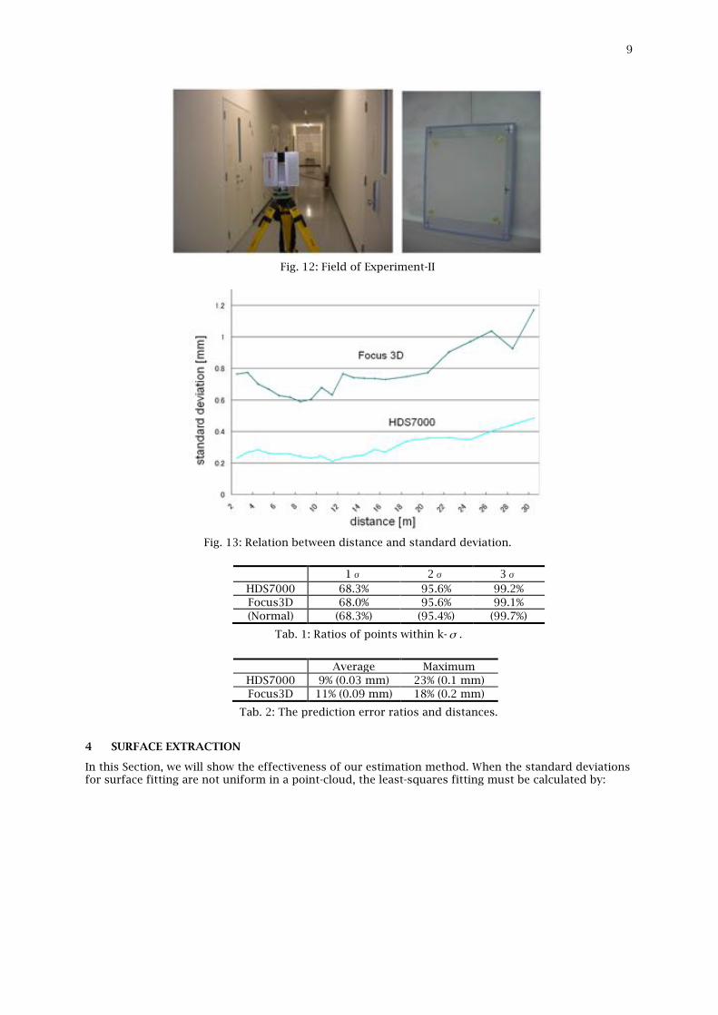
3.4 Experiment - II

Next we perform experiments by using HDS7000 [18] and Focus 3D [19] at the University of Tokyo (Fig. 12). These scanners are currently the state-of-the-art phase-based scanners. In this experiment, we also measured a whiteboard in the same way of Experiment-I. Each scanner has several precision levels determined by measurement speed. We used the level of 500 thousand points/sec, which is the same as Experiment-I.

Fig. 13 show experimental results. Residuals are much smaller than Imager 5003 and the increase rates are also much smaller. The ranges of standard deviations are [0.2, 0.5] for HDS 7000, and [0.6, 1.2] for Focus 3D.

We investigated the rates of k-σ in the both cases, as shown in Tab. 1. The result shows that ratios are consistent with the normal distribution.

We also investigated whether Eqn. (3.3) can be applied to these scanners. Tab. 2 shows the averages and the maximum values of the prediction error and the prediction error ratios. Since the differences are very small, we can conclude that Eqn. (3.3) produces good estimates of the standard deviations even for the latest phase-based scanners.

9

Fig. 12: Field of Experiment-II

Fig. 13: Relation between distance and standard deviation.

� 1� 2� 3� HDS7000 68.3% 95.6% 99.2% Focus3D 68.0% 95.6% 99.1% (Normal) (68.3%) (95.4%) (99.7%)

Tab. 1: Ratios of points within k-σ .

� Average Maximum

HDS7000 9% (0.03 mm) 23% (0.1 mm) Focus3D 11% (0.09 mm) 18% (0.2 mm)

Tab. 2: The prediction error ratios and distances.

4 SURFACE EXTRACTION

In this Section, we will show the effectiveness of our estimation method. When the standard deviations for surface fitting are not uniform in a point-cloud, the least-squares fitting must be calculated by:

10

s(pi )2

σ i2 →min

i=0

n

∑ . (4.1)

In this equation, iσ acts as the weight value; the larger the measurement error is, the smaller impact

the point has on the result.

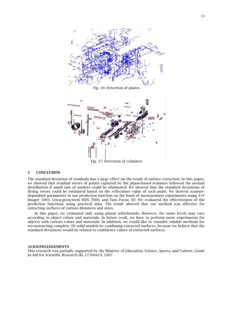
Fig. 14 is an example of point-cloud data, which consists of 33 million points. This point-cloud was captured by Z+F Imager 5003. The angle spacing is 0.036 degree both for the azimuth and the zenith angles. We use Eqn. (3.5) to estimate the standard deviation at each point.

Fig. 15 shows the continuous regions that have been segmented using the thresholds derived by Eqn. (2.1). Each region is shown in a different color. Our spacing parameters extract effectively the objects of various sizes and distances.

Fig. 16 and Fig. 17 show planes and cylinders extracted by the region growing method. The seed regions were randomly selected in each continuous region, and surface equations are calculated using Eqn. (4.1). The region growing requires the on/not-on check for each point. We used 2σ as the threshold. The result shows that our prediction function works well for extracting surfaces of various distances and sizes.

Fig. 14: Example point-cloud

Fig. 15: Detection of continuous regions

11

Fig. 16: Detection of planes

Fig. 17: Detection of cylinders

5 CONCLUSION

The standard deviation of residuals has a large effect on the result of surface extraction. In this paper, we showed that residual errors of points captured by the phase-based scanners followed the normal distribution if small rate of outliers could be eliminated. We showed that the standard deviations of fitting errors could be estimated based on the reflectance value of each point. We derived scanner-dependent parameters in our prediction function on the basis of measurement experiments using Z+F Imager 5003, Leica-geosystem HDS 7000, and Faro Focus 3D. We evaluated the effectiveness of the prediction functions using practical data. The result showed that our method was effective for extracting surfaces of various distances and sizes.

In this paper, we estimated only using planar whiteboards. However, the noise levels may vary according to object colors and materials. In future work, we have to perform more experiments for objects with various colors and materials. In addition, we would like to consider reliable methods for reconstructing complete 3D solid models by combining extracted surfaces, because we believe that the standard deviations would be related to confidence values of extracted surfaces. ACKNOWLEDGEMENTS This research was partially supported by the Ministry of Education, Science, Sports, and Culture, Grant-in-Aid for Scientific Research (B), 17360414, 2007.

12

REFERENCES

[1] Yang, M.; Lee, E.: Segmentation of measured point data using a parametric quadric surface approximation. Computer-Aided Design 31(7), 1999, 449–457.

[2] Mangan, A.P.; Whitaker, R.T.: Partitioning 3D surface meshes using watershed segmentation. IEEE Transactions on Visualization and Computer Graphics 5(4), 1999, 308–321.

[3] Shami, A.: A survey on mesh segmentation techniques, Computer Graphics Forum, 27(6), 2008, 1539-1556.

[4] Rusu, R., B.; Marton, Z., C.; Blodow, N.; Dolha, M.; Beetz, M.: Towards 3D Object Maps for Autonomous Household Robots , Proc. of the 20th IEEE International Conference on Intelligent Robots and Systems, 2007.

[5] Belton, D.; Lichti, D., D.: Classification and segmentation of terrestrial laser scanner point clouds using local variance information, ISPRS Symposium: Image Engineering and Vision Methodology, 2006, 44-49.

[6] Lukacs, G.; Marshall, A.D.; Martin, R.R.: Faithful least-squares fitting of spheres, cylinders, cones and tori for reliable segmentation. Proceedings, 5th European Conference on Computer Vision, 1998, 671–686.

[7] Stewart, C.V.: Robust Parameter Estimation in Computer Vision. SIAM Review 41(3), 1999, 513–537.

[8] Masuda, H.; Tanaka, I.: Extraction of Surface Primitives from Noisy Large-Scale Point-Clouds, Computer-Aided Design & Applications, 6(3), 2009, 47-57.

[9] Schnabel, R.; Wahl, R.; Klein, R.: Efficient RANSAC for Point-Cloud Shape Detection, Computer Graphics Forum, 26(2), 2007, 214-226.

[10] Torr, P. H. S.: MLESAC: A New Robust Estimator with Application to Estimating Image Geometry, Computer Vision and Image Understanding, 78, 2000, 138-156.

[11] Levin, D.: Mesh-independent surface interpolation. Geometric Modeling for Scientific Visualization, 2003, 37–49.

[12] Sharf, Q.; Sharf, A.; Wan, G.; Li, Y.; Mitra, N., Cohen-Or, D., Chen, B. : Non-local Scan Consolidation for 3D Urban Scenes, ACM Trans. Graph. 29(4), 2010, Article 94.

[13] Kersten, T., P.; Mechelke, K.; Geometric Accuracy Investigations of the Latest Terrestrial Laser Scanning Systems, Proc. of FIG Working Week, 2008.

[14] Mitra, N., J.; Nguyen, A.: Estimating Surface Normals in Noisy Point Cloud Data, Symposium on Computational Geometry'03, 2003, 322-328.

[15] Huber, P.J.: Robust Statistics. Wiley Series in Probability and Statistics, Wiley-Interscience, 2003. [16] Sun, X.; Rosin, P. L.; Martin R. R.: Noise Analysis and Synthesis for 3D Laser Depth Scanners,

Graphics Models 71, 2009, 34-48. [17] Technical Data IMAGER, http://www.zf-laser.com, Zoller-Fröhligh. [18] HDS7000 Datasheet, http://www.leica-geosystems.com, Leica-Geosystem. [19] FARO Laser Scanner Focus 3D Techsheet, http://www.faro.com, Faro.