http://optics.hanyang.ac.kr/~shsong송석호 (물리학과)

Field and Wave Electromagnetics, David K. ChengReviews on

(Week 1) 2. Vector Analysis3. Static Electric Fields

(Week 2) 4. Solution of Electrostatic Problems5. Steady Electric Currents

(Week 3) 6. Static Magnetic Fields7. Time-varying Fields: Faraday’s Law

Introduction to Electromagnetics, 3rd Edition, David J. Griffiths(Week 4-5) 7. Electrodynamics: Maxwell’s Equations(Week 6) 8. Conservation Laws(Week 7-8) 9. Electromagnetic Waves(Week 9-10) 10. Potentials and Fields(Week 11-12) 11. Radiation(Week 13-14) 12. Electrodynamics and Relativity

Chapter 4. Solution of Electrostatic

Problems한양대학교 전기공학과

정진욱

2

, V

V V

E D

E

2 2 22

2 2 2

2 2 3 1 3 1 2

1 2 3 1 1 1 2 2 2 3 3 3

In generalized coordinate,

1

x y z

h h h h h hh h h u h u u h u u h u

(Laplacian)

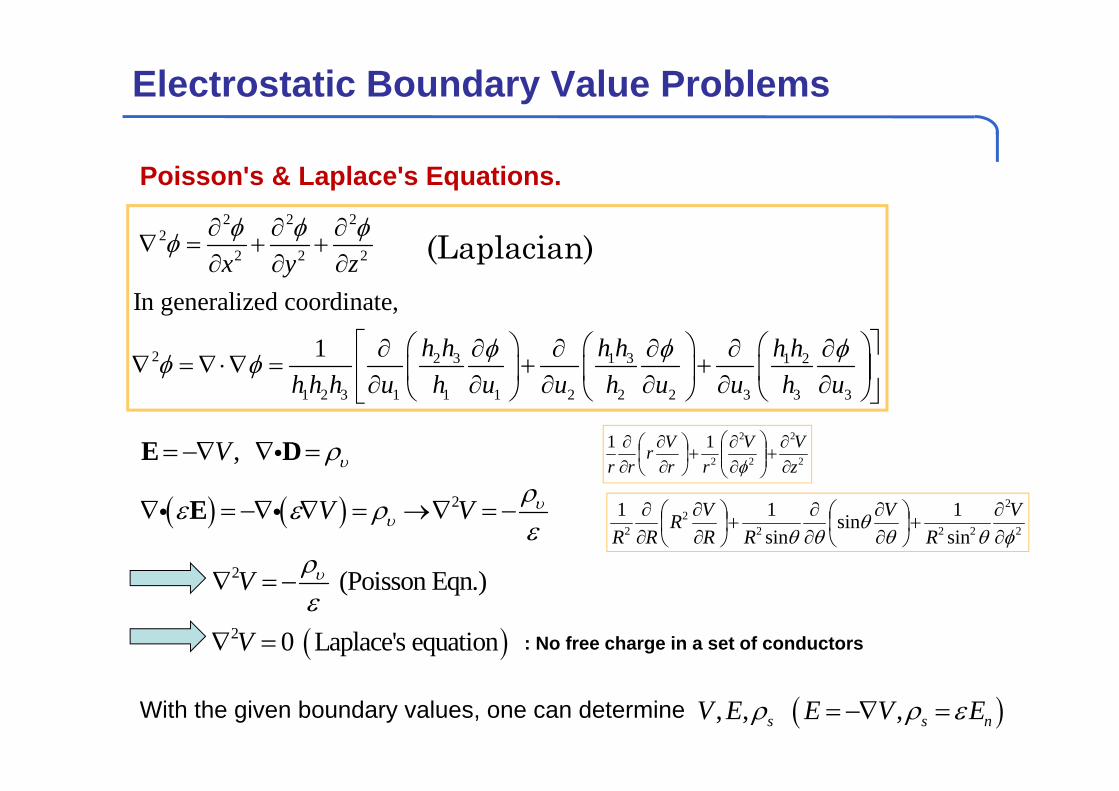
Electrostatic Boundary Value Problems

Poisson's & Laplace's Equations.

2 (Poisson Eqn.)V

2 0 Laplace's equationV : No free charge in a set of conductors

2

2

2

2

2

11zVV

rrVr

rr

2

2

2222

2 sin1sin

sin11

V

RV

RRVR

RR

With the given boundary values, one can determine , , ,s s nV E E V E

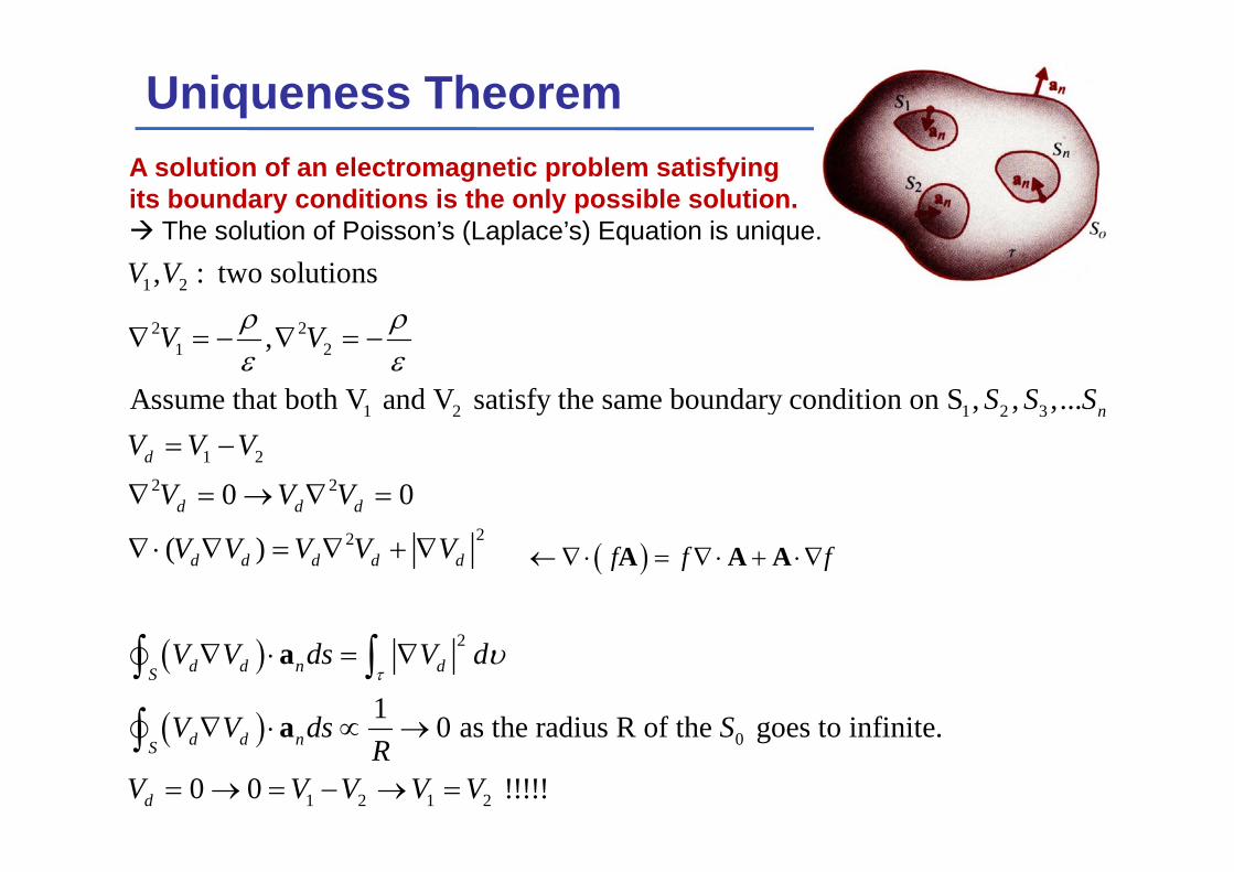
Uniqueness Theorem

1 2

2 21 2

1 2 1 2 3

1 22 2

22

2

, : two solutions

,

Assume that both V and V satisfy the same boundary condition on S , , ,...

0 0

( )

1

n

d

d d d

d d d d d

d d n dS

d d nS

V V

V V

S S SV V V

V V V

V V V V V

V V ds V d

V V dsR

a

a

0

1 2 1 2

0 as the radius R of the goes to infinite.

0 0 !!!!!d

S

V V V V V

A A Af f f

A solution of an electromagnetic problem satisfying its boundary conditions is the only possible solution. The solution of Poisson’s (Laplace’s) Equation is unique.

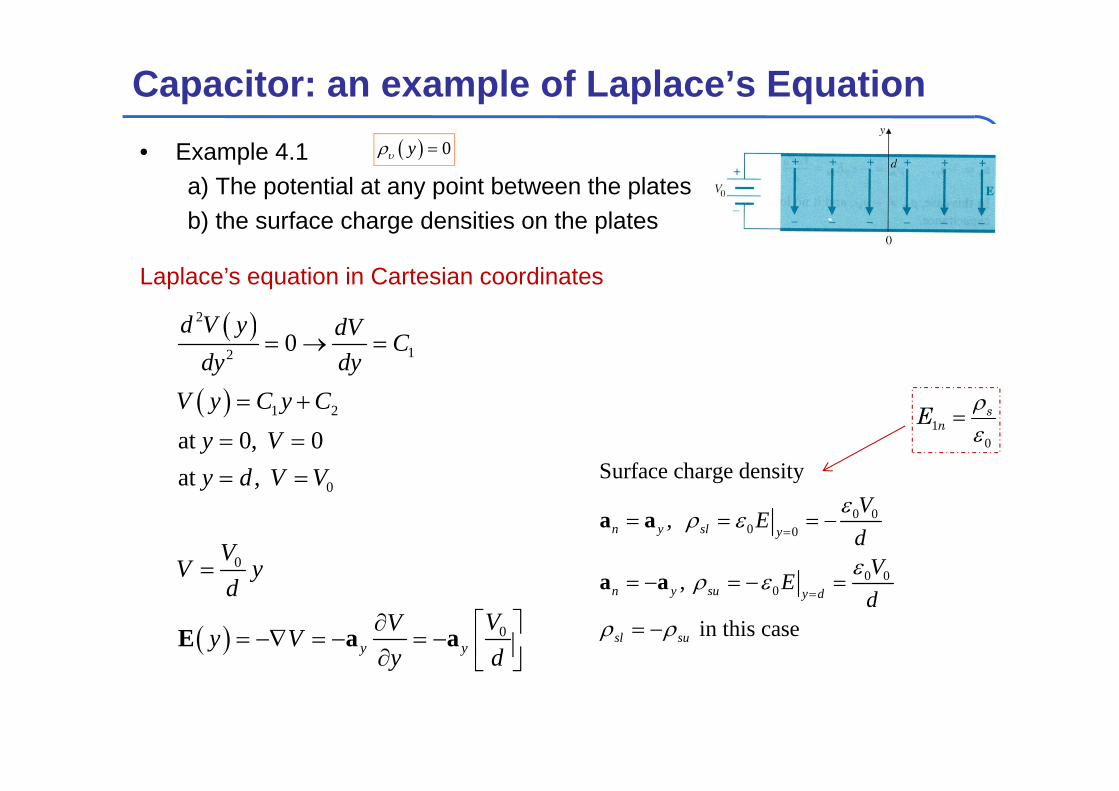
Capacitor: an example of Laplace’s Equation• Example 4.1

a) The potential at any point between the platesb) the surface charge densities on the plates

0 y

2

12

1 2

0

0

0

0

at 0, 0at ,

y y

d V y dV Cdydy

V y C y Cy Vy d V V

VV y

dVVy V

y d

E a a

0 00 0

0 00

Surface charge density

,

,

in this case

a a

a a

n y sl y

n y su y d

sl su

VE

dV

Ed

10

snE

Laplace’s equation in Cartesian coordinates

Electrostatic Boundary Value Problems

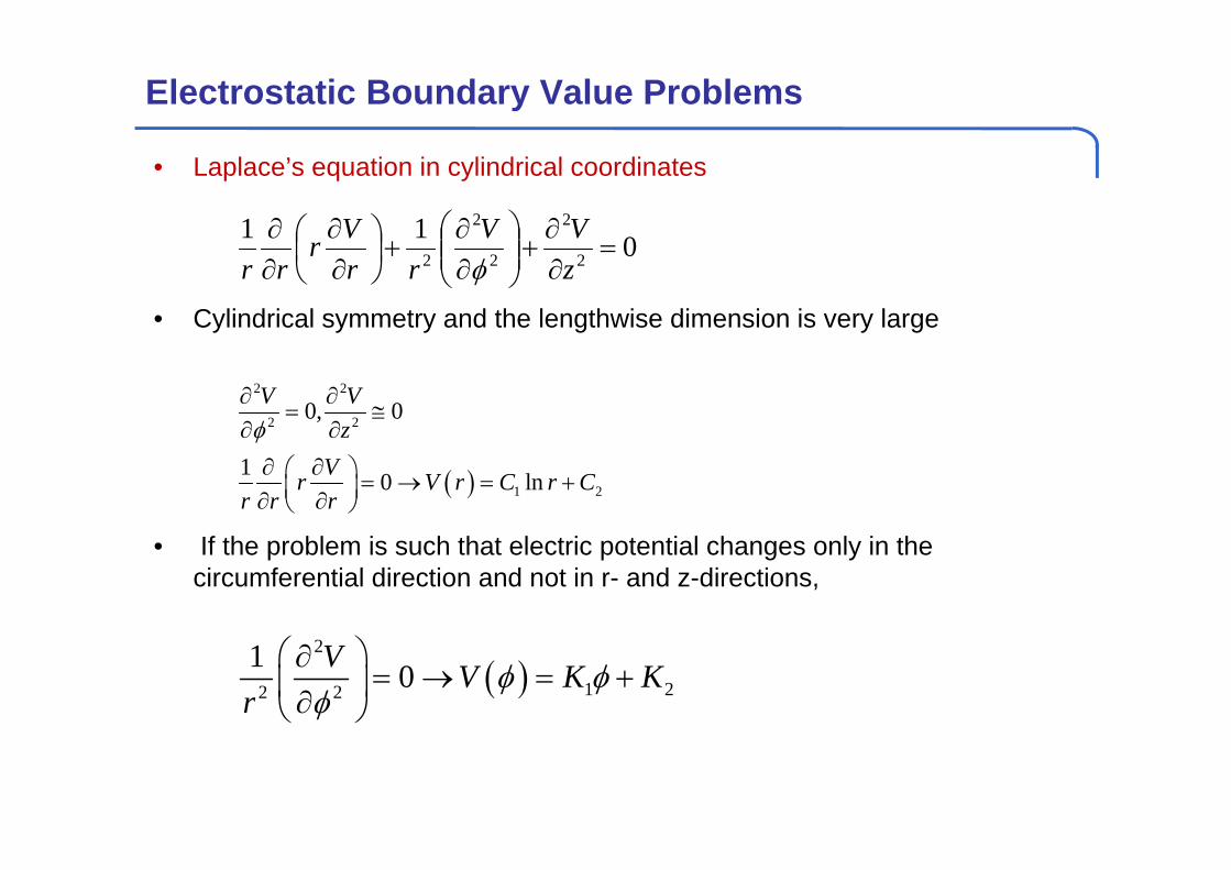
• Laplace’s equation in cylindrical coordinates

• Cylindrical symmetry and the lengthwise dimension is very large

• If the problem is such that electric potential changes only in the circumferential direction and not in r- and z-directions,

0112

2

2

2

2

zVV

rrVr

rr

2 2

2 2

1 2

0, 0

1 0 ln

V Vz

Vr V r C r Cr r r

2

1 22 2

1 0V V K Kr

Electrostatic Boundary Value Problems

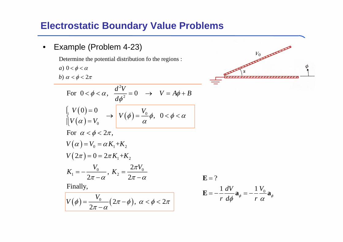
• Example (Problem 4-23)

aaE

E

011?

Vrd

dVr

Determine the potential distribution fo the regions : ) 0) 2

ab

2

2

0

0

0 1 2

1 2

0 01 2

0

For 0 , 0

0 0 , 0

For 2 , +

2 0 2 +2

, 2 2

Finally,

2 , 22

d V V A Bd

V VV

V V

V V K K

V K KV V

K K

VV

Electrostatic Boundary Value Problems

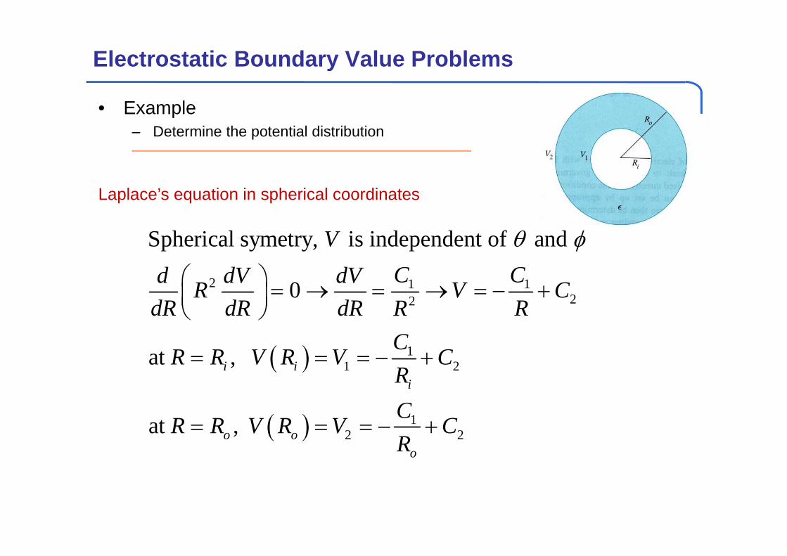
• Example – Determine the potential distribution

2 1 122

11 2

12 2

Spherical symetry, is independent of and

0

at ,

at ,

i ii

o oo

VC Cd dV dVR V C

dR dR dR RRC

R R V R V CRC

R R V R V CR

Laplace’s equation in spherical coordinates

Electrostatic Boundary Value Problems

0 1 2 0 2 11 2

0 0

01 2 0 2 1 0

0

,

1 ,

is independent of the dielectric constant of the insulating material

i i

i i

ii i

i

R R V V R V RVC C

R R R RR R

V R V V R V RV R R RR R R

V

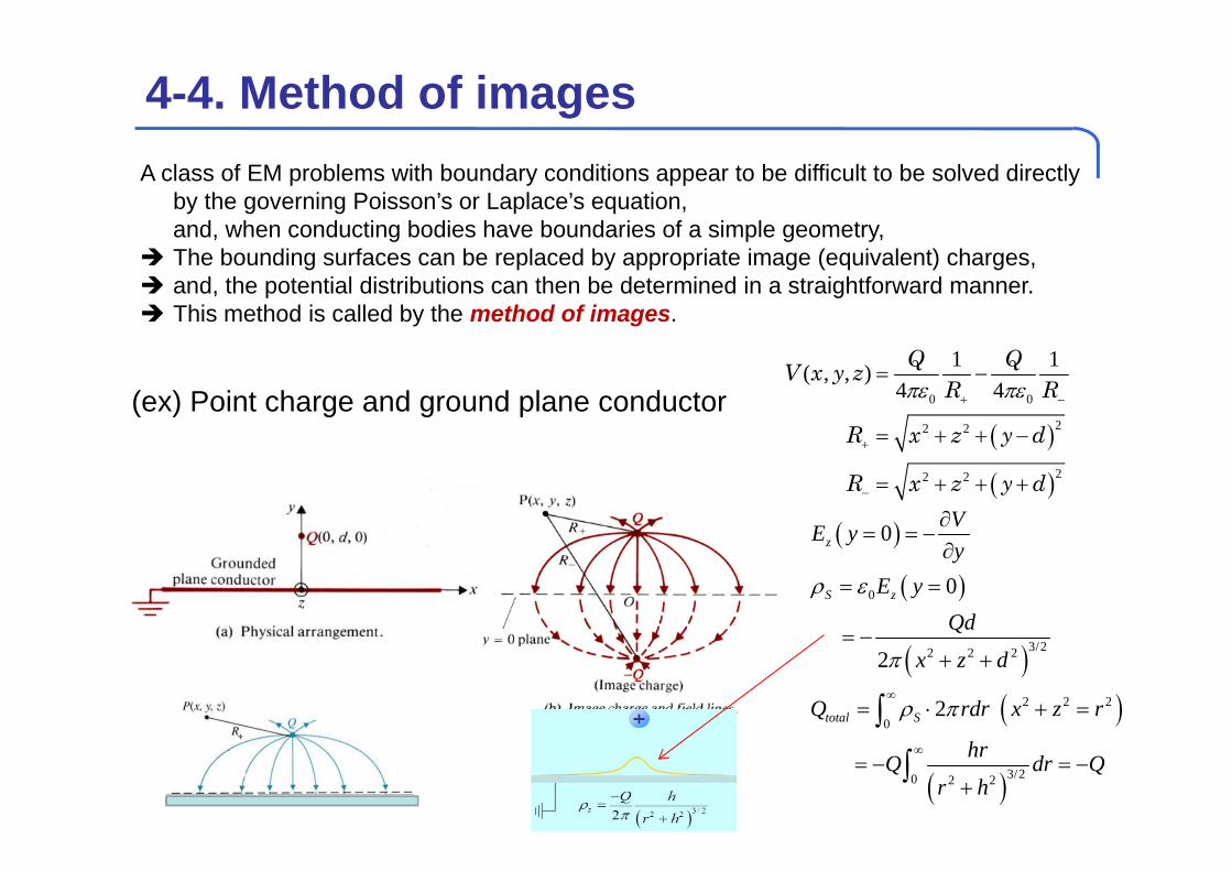
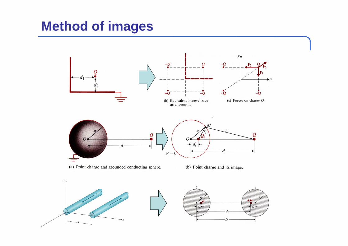
4-4. Method of images

(ex) Point charge and ground plane conductor

A class of EM problems with boundary conditions appear to be difficult to be solved directlyby the governing Poisson’s or Laplace’s equation,and, when conducting bodies have boundaries of a simple geometry,

The bounding surfaces can be replaced by appropriate image (equivalent) charges, and, the potential distributions can then be determined in a straightforward manner. This method is called by the method of images.

0 0

22 2

22 2

1 1( , , )4 4

Q QV x y zR R

R x z y d

R x z y d

0

3/22 2 2

2 2 2

0

3/20 2 2

0

0

2

2

z

S z

total S

VE yy

E yQd

x z d

Q rdr x z r

hrQ dr Qr h

Method of images

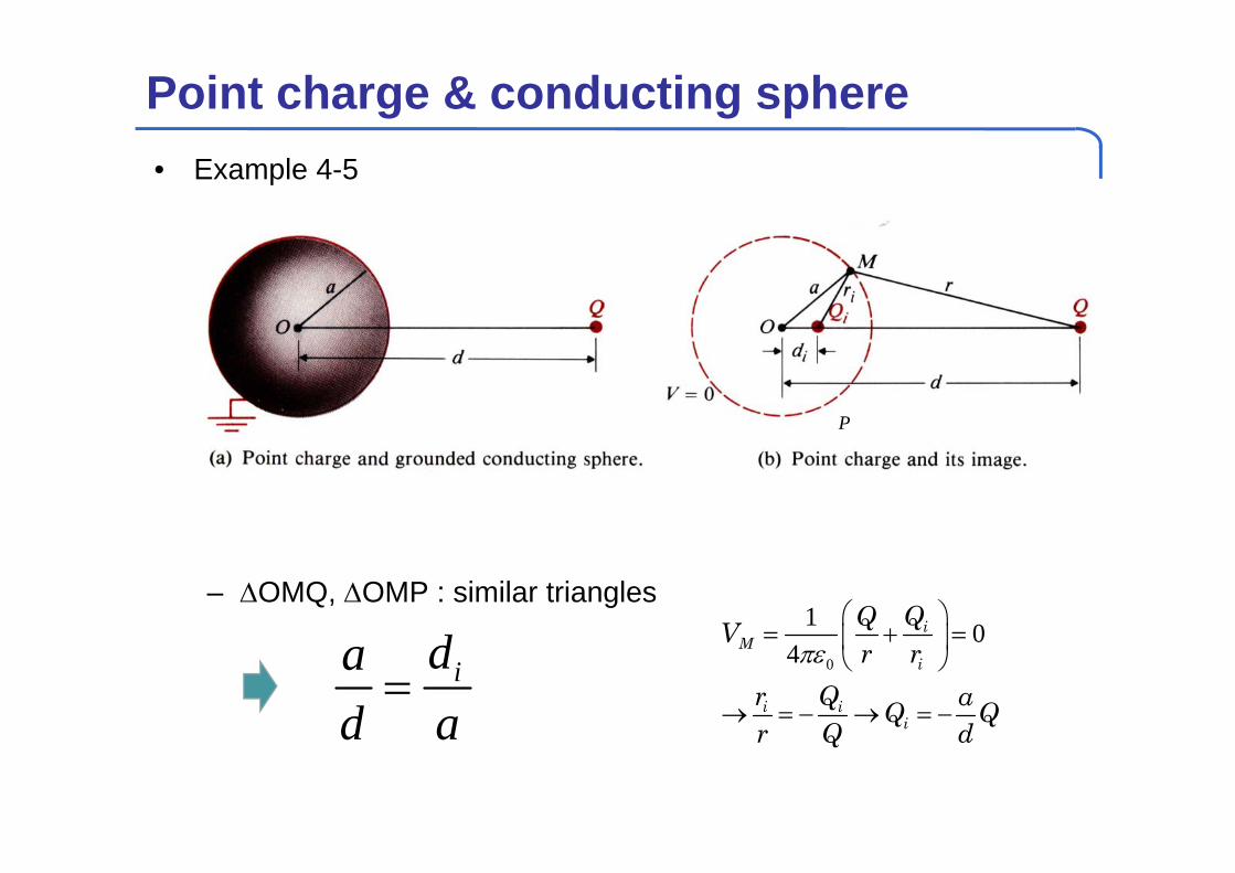
• Example 4-5

– OMQ, OMP : similar triangles

Point charge & conducting sphere

idad a

P

0

1 04

iM

i

i ii

QQVr r

r Q aQ Qr Q d

0

2 2 2 2

2 2 2 20

2

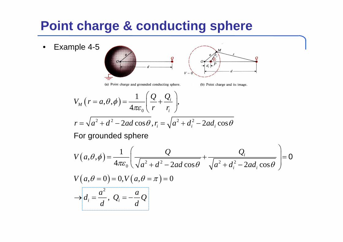
1, , ,4

2 cos , 2 cos

1, ,4 2 cos 2 cos

, 0 0, , 0

,

For grounded sphere

0

iM

i

i i i

i

i i

i i

QQV r ar r

r a d ad r a d ad

QQV aa d ad a d ad

V a V a

a ad Q Qd d

Point charge & conducting sphere• Example 4-5

P

0

2 2

22 22

2 2

0 3/ 22 2

2

1 1, ,4

2 cos ,

2 cos

,

,4 2 cos

s

ind

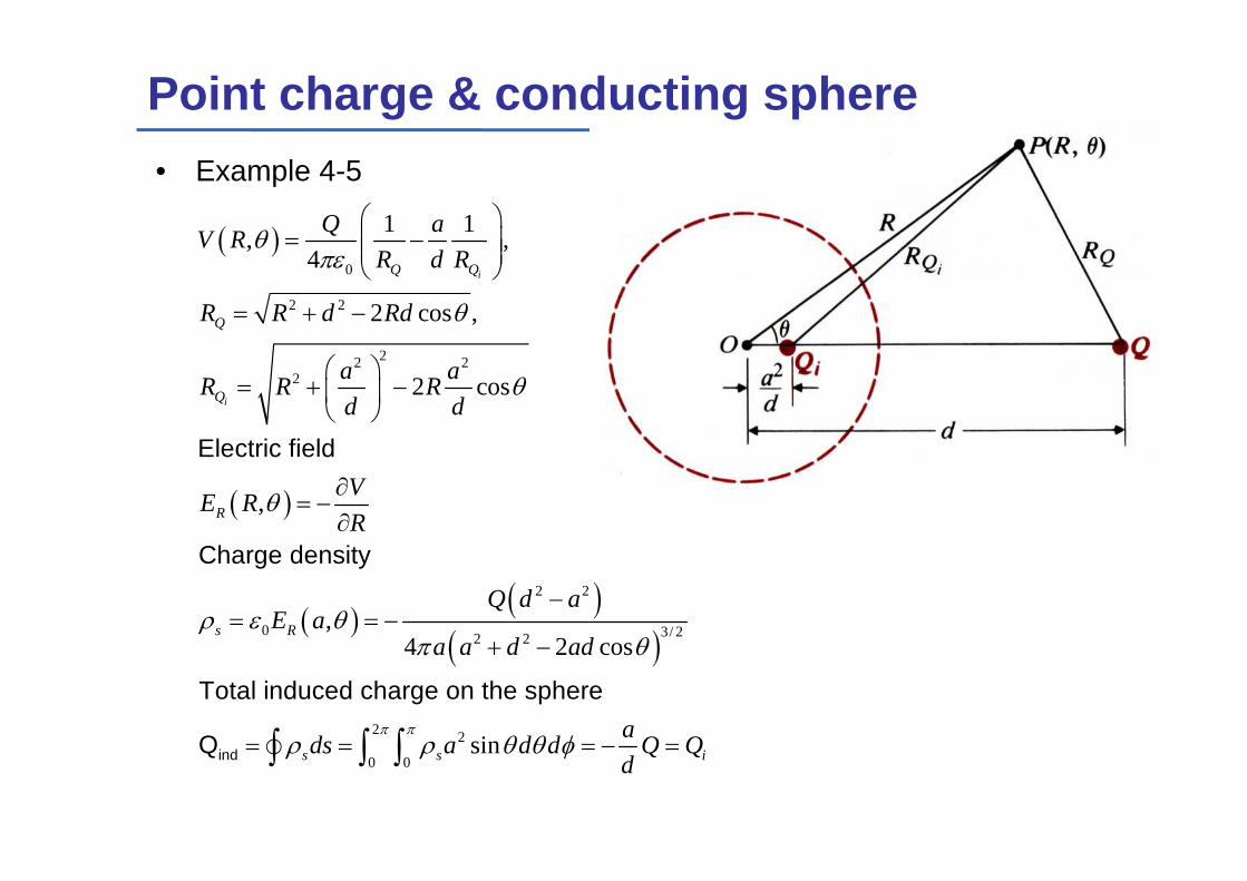
Electric field

Charge density

Total induced charge on the sphere

Q

i

i

Q Q

Q

Q

R

s R

s s

Q aV RR d R

R R d Rd

a aR R Rd d

VE RR

Q d aE a

a a d ad

ds a2

0 0in

i

ad d Q Qd

Point charge & conducting sphere• Example 4-5

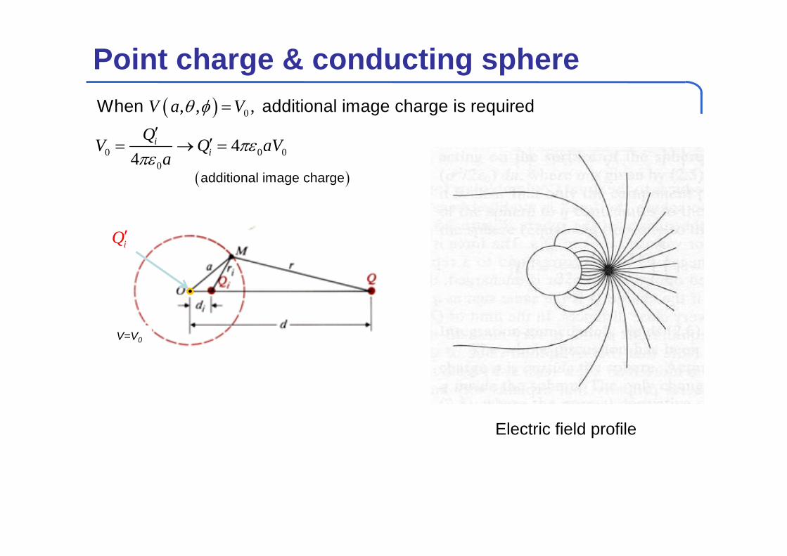
Point charge & conducting sphere 0

0 0 00

, , ,

44

ii

V a VQV Q aV

a

When additional image charge is required

Electric field profile

additional image charge

V=V0

iQ

Chapter 5Steady Electric Currents

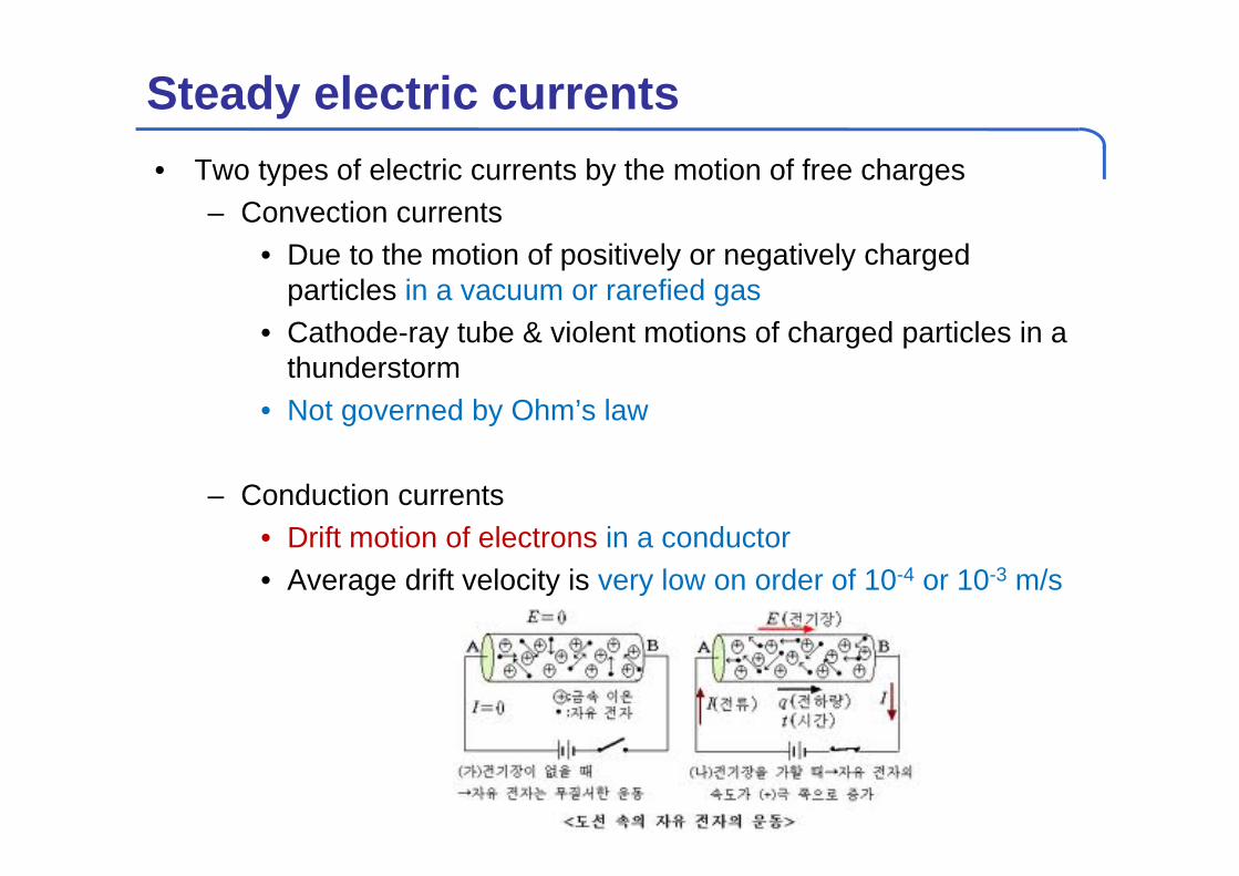
Steady electric currents• Two types of electric currents by the motion of free charges

– Convection currents• Due to the motion of positively or negatively charged

particles in a vacuum or rarefied gas• Cathode-ray tube & violent motions of charged particles in a

thunderstorm• Not governed by Ohm’s law

– Conduction currents• Drift motion of electrons in a conductor• Average drift velocity is very low on order of 10-4 or 10-3 m/s

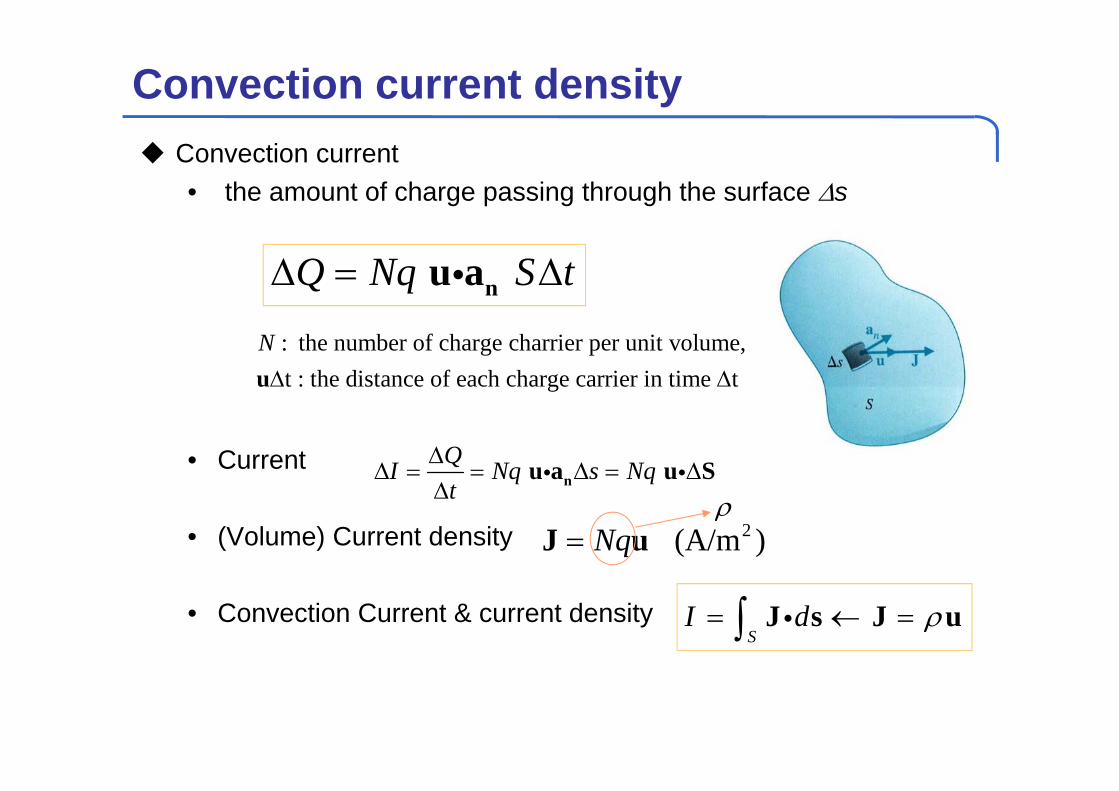
Convection current density Convection current

• the amount of charge passing through the surface s

• Current

• (Volume) Current density

• Convection Current & current density

: the number of charge charrier per unit volume, t : the distance of each charge carrier in time t

N u

Q Nq S t nu a

QI Nq s Nqt

nu a u S

2 (A/m )NqJ u

SI d J s J u

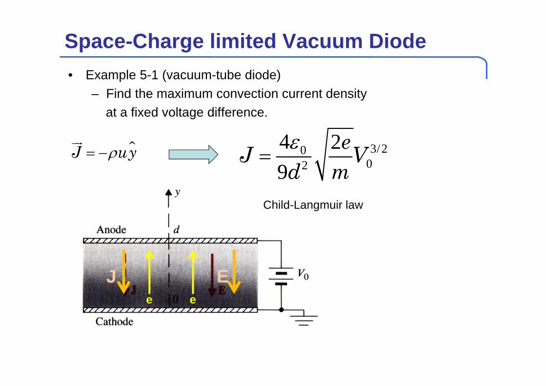
Space-Charge limited Vacuum Diode• Example 5-1 (vacuum-tube diode)

– Find the maximum convection current density at a fixed voltage difference.

3/2002

4 29

eJ Vd m

e e

J E

J uy

Child-Langmuir law

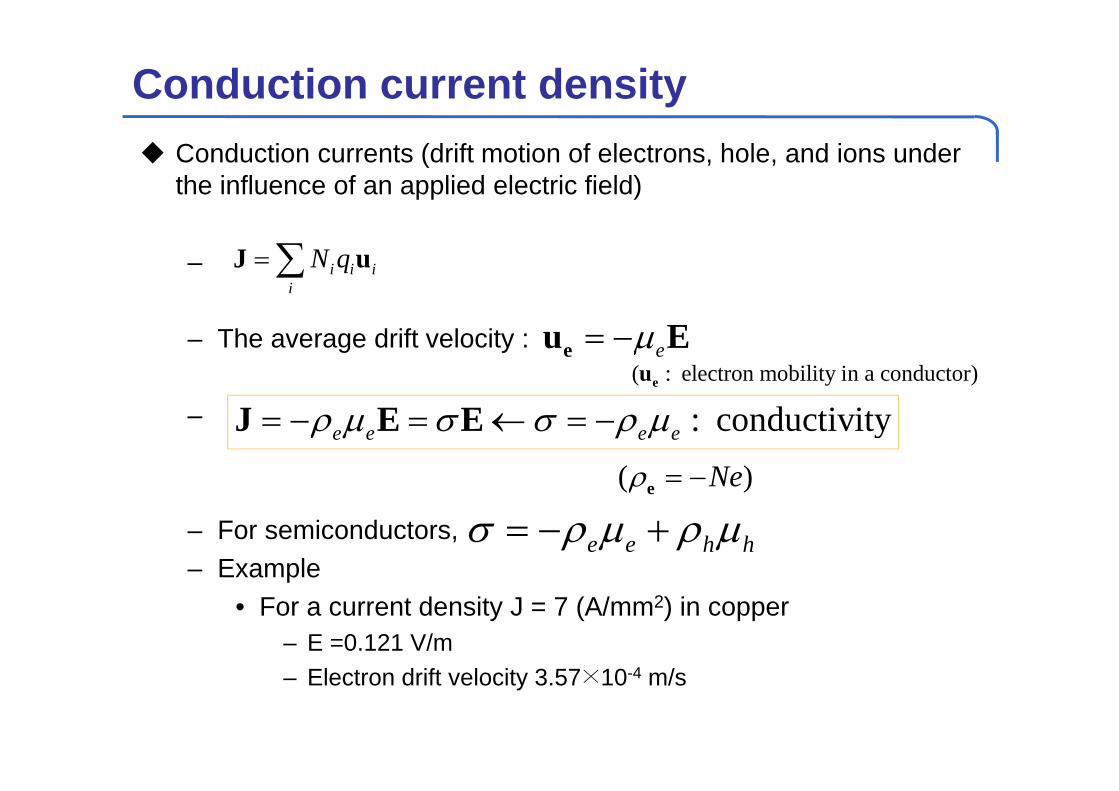
Conduction current density Conduction currents (drift motion of electrons, hole, and ions under

the influence of an applied electric field)

–

– The average drift velocity :

–

– For semiconductors, – Example

• For a current density J = 7 (A/mm2) in copper– E =0.121 V/m– Electron drift velocity 3.57×10-4 m/s

i i ii

N q J u

e eu E

: conductivitye e e e J E E

e e h h

( : electron mobility in a conductor)eu

( )Ne e

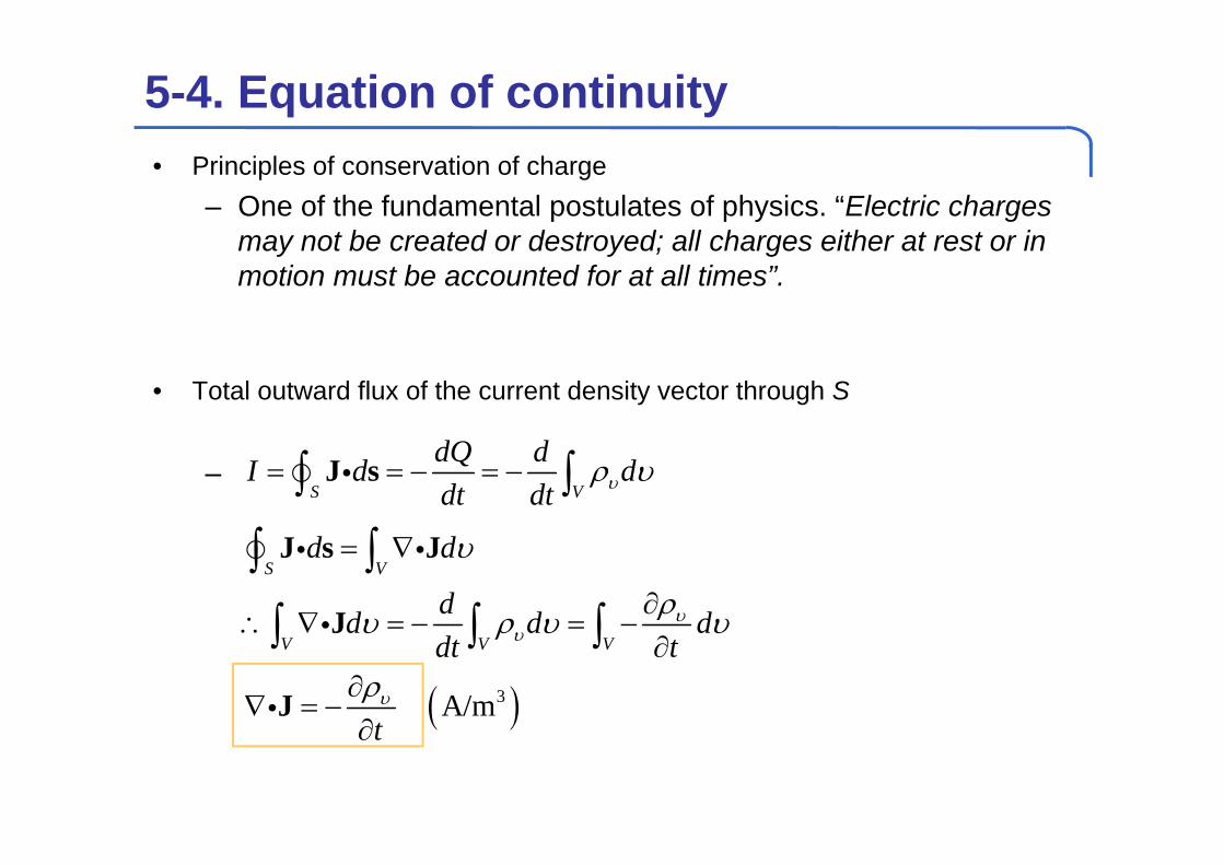
5-4. Equation of continuity• Principles of conservation of charge

– One of the fundamental postulates of physics. “Electric charges may not be created or destroyed; all charges either at rest or in motion must be accounted for at all times”.

• Total outward flux of the current density vector through S

–

3 A/m

S V

S V

V V V

dQ dI d ddt dt

d d

dd d ddt t

t

J s

J s J

J

J

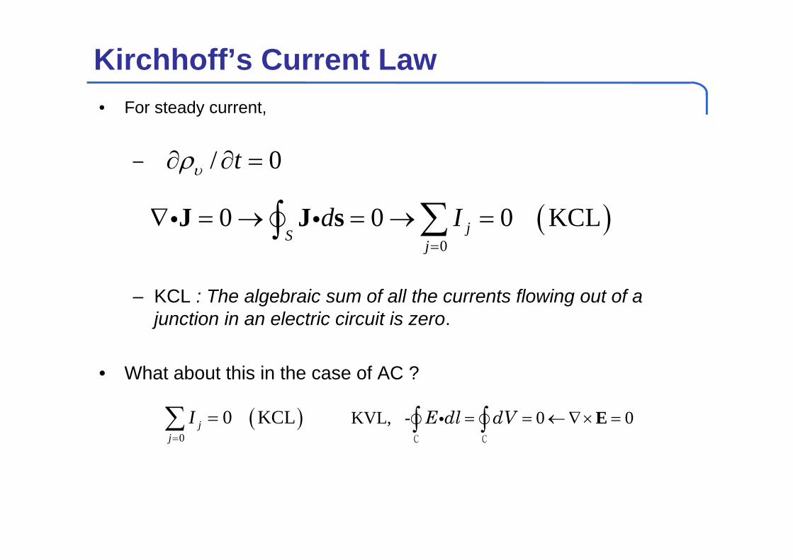
Kirchhoff’s Current Law• For steady current,

–

– KCL : The algebraic sum of all the currents flowing out of a junction in an electric circuit is zero.

• What about this in the case of AC ?

/ 0t

0

0 0 0 KCLjSj

d I

J J s

0

0 KCL

jj

I KVL, - 0 0E dl dV E C C

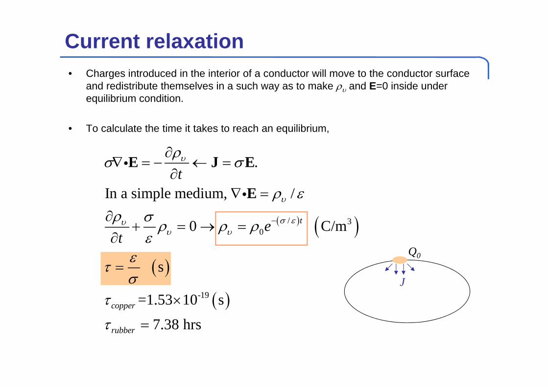
Current relaxation• Charges introduced in the interior of a conductor will move to the conductor surface

and redistribute themselves in a such way as to make and E=0 inside under equilibrium condition.

• To calculate the time it takes to reach an equilibrium,

/ 30

-19

.

In a simple medium, /

0 C/m

s

=1.53 10 s

7.38 hrs

t

copper

rubber

t

et

E J E

E

Q0

J

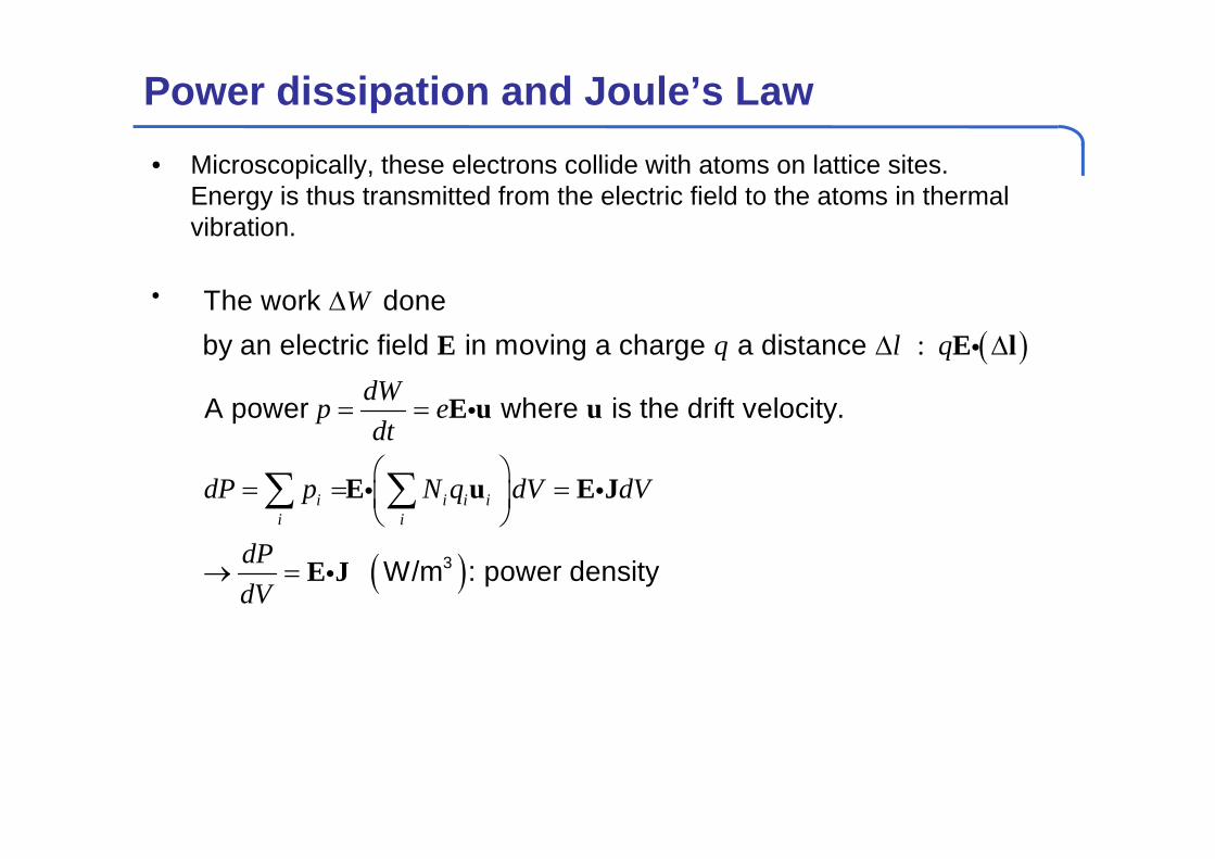
Power dissipation and Joule’s Law• Microscopically, these electrons collide with atoms on lattice sites.

Energy is thus transmitted from the electric field to the atoms in thermal vibration.

•

:

E E l

E u u

E u E J

E J

i i i ii i

Wq l q

dWp edt

dP p N q dV dV

dPdV

3

The work done by an electric field in moving a charge a distance

A power where is the drift velocity.

W/m : power density

2

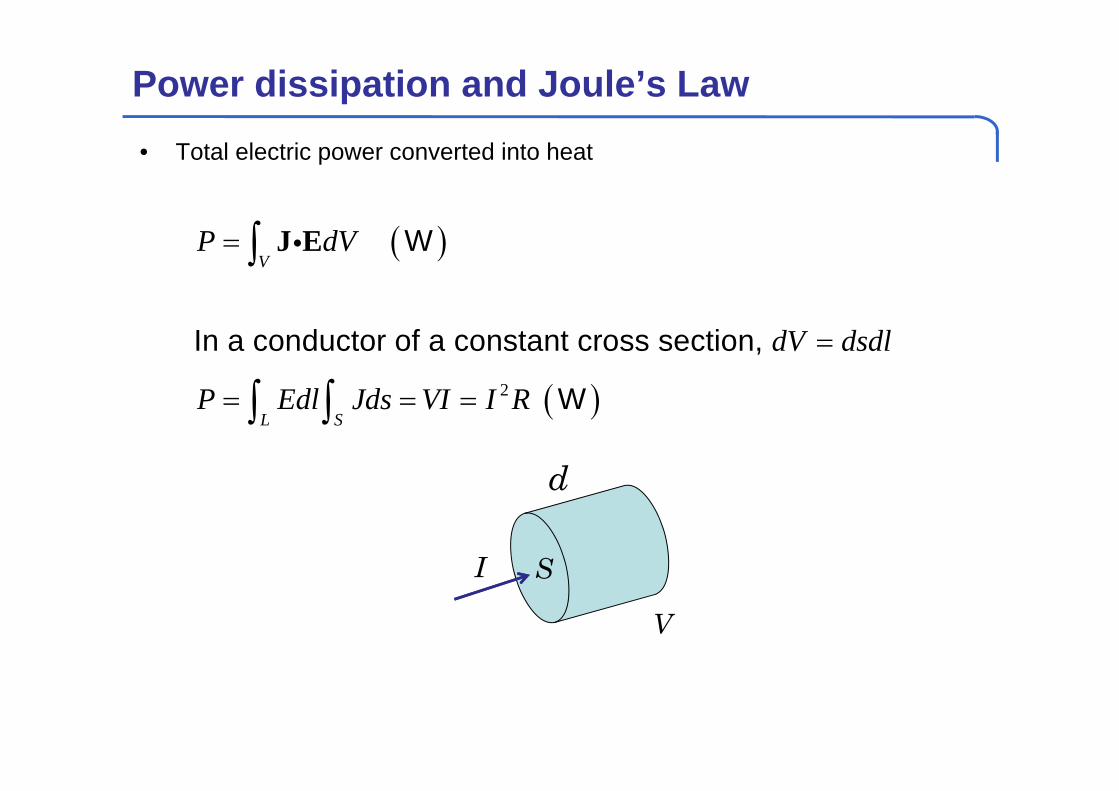
J EV

L S

P dV

dV dsdl

P Edl Jds VI I R

W

In a conductor of a constant cross section,

W

Power dissipation and Joule’s Law• Total electric power converted into heat

d

V

I S

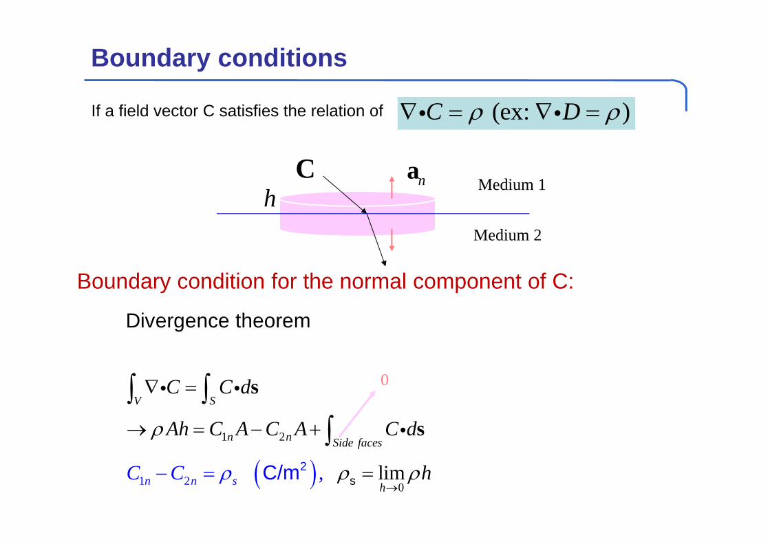
Boundary conditions

Boundary condition for the normal component of C:

1 2

01 2 l, im

V S

n n Side face

n s hn

s

C C d

Ah C A C A C

C

d

hC

s

s

2

s

Divergence theore

C m

m

/

0

naCMedium 1

Medium 2

h

If a field vector C satisfies the relation of (ex: )C D

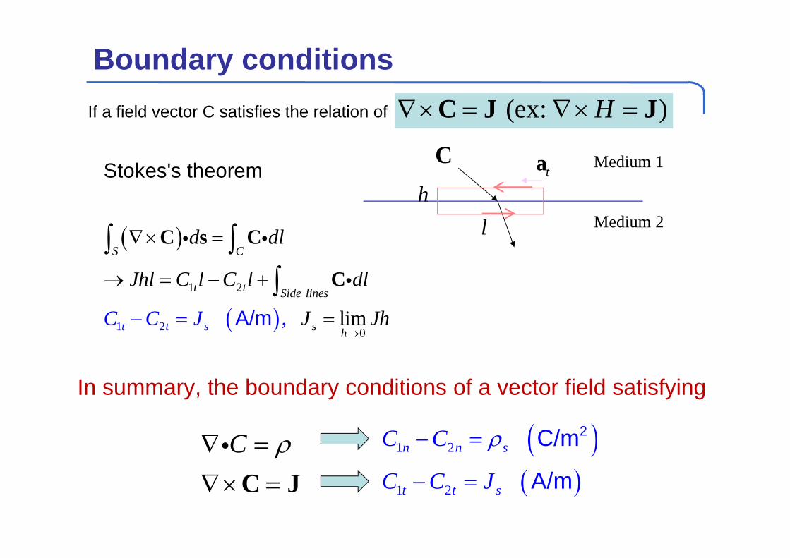
Boundary conditions(ex: )H C J J

2

1

1

02 lim,

S C

t t Side line

t t

s

s hs

d dl

Jhl C l C l dl

JC C J Jh

C s C

C

Stokes's th

A/

e

m

e

or m

Medium 2

taCh

l

Medium 1

1 2

1 2

n n s

t t s

C C

C C J

2 C/m

A/m

In summary, the boundary conditions of a vector field satisfying

If a field vector C satisfies the relation of

C C J

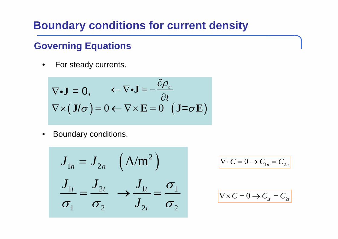
Governing Equations

• For steady currents.

• Boundary conditions.

21 2

1 2 1 1

1 2 2 2

A/m

n n

t t t

t

J J

J J JJ

0 0 = 0,

/ =

JJ E J E

Boundary conditions for current density

t

J

1 20 t tC C C

1 20 n nC C C

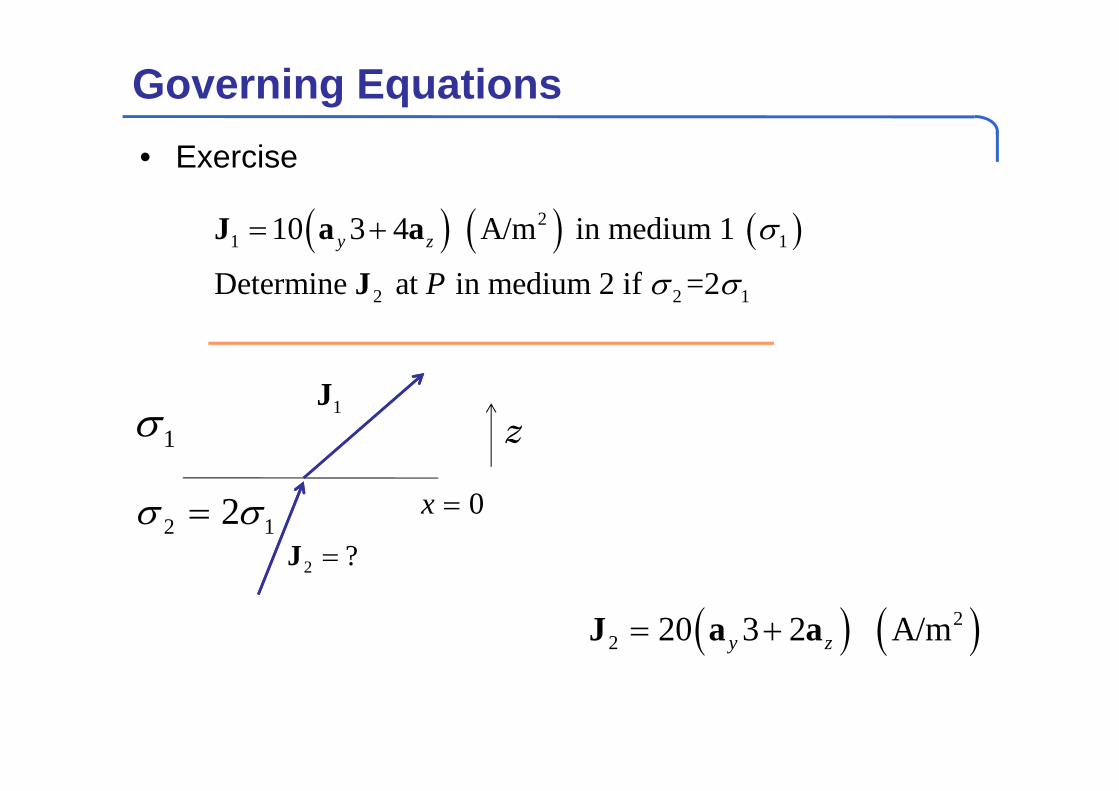
Governing Equations• Exercise

21 1

2 2 1

10 3 4 A/m in medium 1

Determine at in medium 2 if =2

J a a

Jy z

P

1

2 12 0x

22 20 3 2 A/my z J a a

1J

2 ?J

z

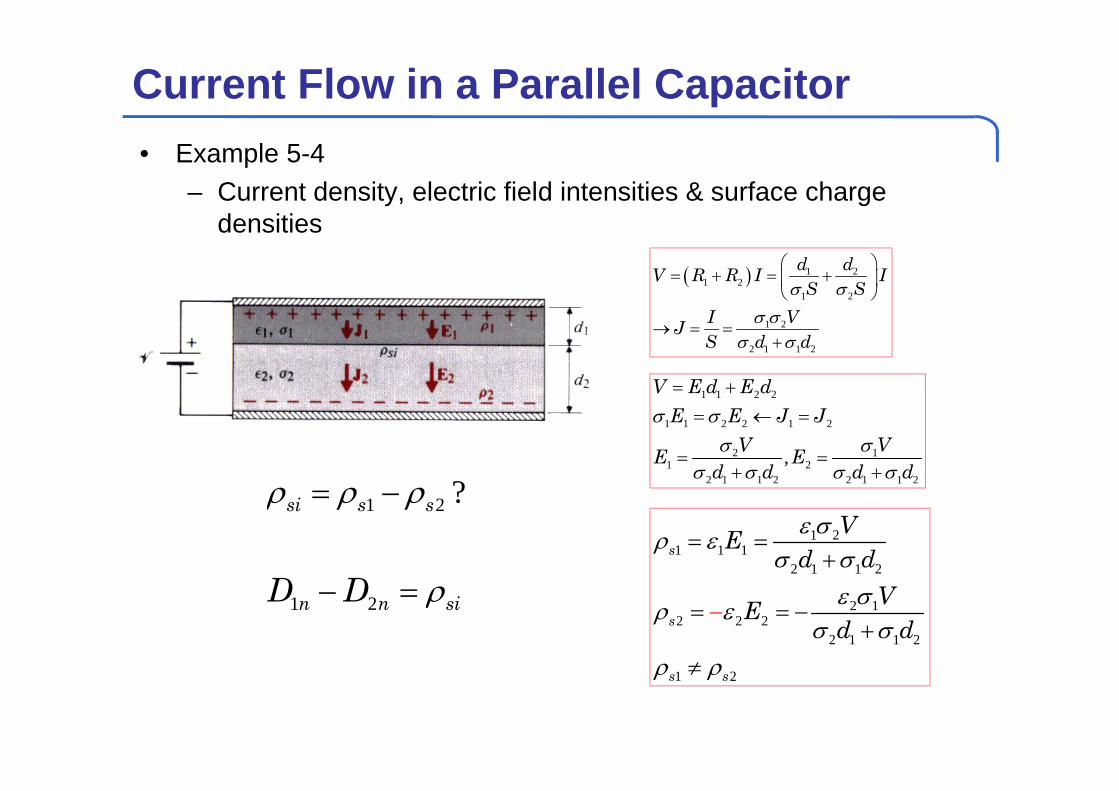
Current Flow in a Parallel Capacitor• Example 5-4

– Current density, electric field intensities & surface charge densities

1 21 2

1 2

1 2

2 1 1 2

d dV R R I IS S

VIJS d d

1 1 2 2

1 1 2 2 1 2

2 11 2

2 1 1 2 2 1 1 2

,

V E d E dE E J J

V VE Ed d d d

1 21 1 1

2 1 1 2

2 12 2 2

2 1 1 2

1 2

s

s

s s

VEd d

VEd d

1 2

1 2

?si s s

n n siD D

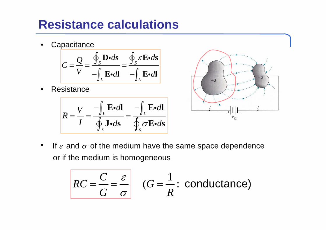
Resistance calculations• Capacitance

• Resistance

•

S S

L L

d dQCV d d

D s E s

E l E l

L L

s s

d dVRI d d

E l E l

J s E s

If and of the medium have the same space dependenceor if the medium is homogeneous

CRCG

1( :GR

conductance)

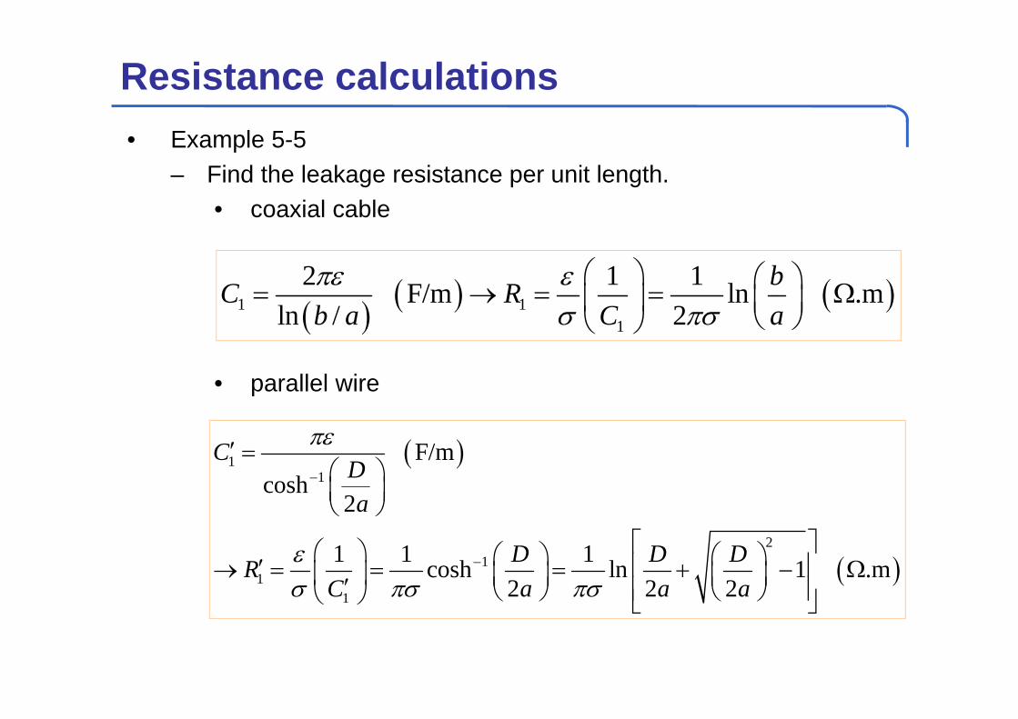
Resistance calculations• Example 5-5

– Find the leakage resistance per unit length.• coaxial cable

• parallel wire

1 11

2 1 1 F/m ln .mln / 2

bC Rb a C a

11

21

11

F/mcosh

2

1 1 1cosh ln 1 .m2 2 2

CDa

D D DRC a a a

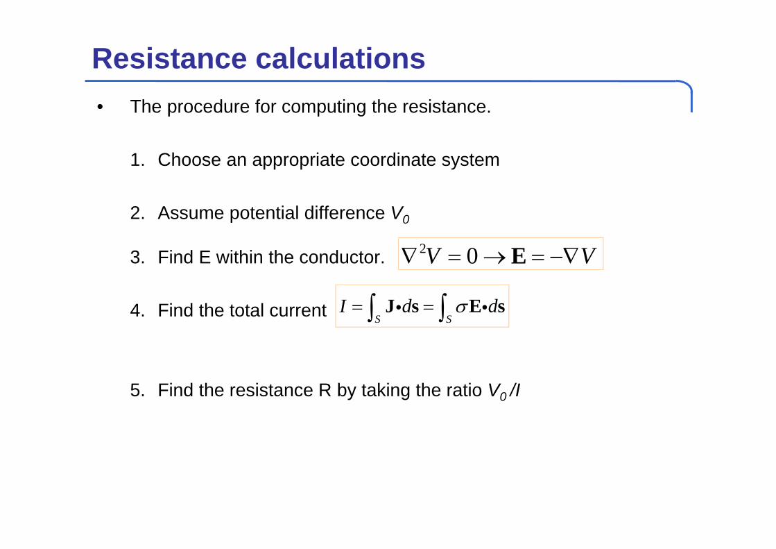
Resistance calculations• The procedure for computing the resistance.

1. Choose an appropriate coordinate system

2. Assume potential difference V0

3. Find E within the conductor.

4. Find the total current

5. Find the resistance R by taking the ratio V0 /I

S SI d d J s E s

2 0V V E

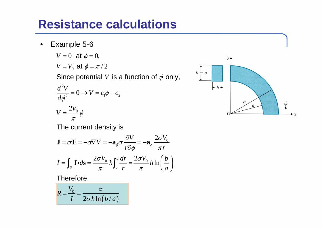
Resistance calculations• Example 5-6

0

2

1 22

0

0

0 0

0

0 0/ 2

0

2

2

2 2 ln

at , at

Since potential is a function of only,

The current density is

Therefore,

J E a a

J sb

S a

VV V

Vd V V c cd

VV

VVVr r

V Vdr bI d h hr a

VRI 2 ln /h b a