scalable computing
TRANSCRIPT

Scalable Computing:Practice and Experience
Scientific International Journalfor Parallel and Distributed Computing
ISSN: 1895-1767
⑦⑦⑦⑦
⑦⑦
t
Volume 19(1) March 2018
Editor-in-Chief
Dana Petcu
Computer Science Department
West University of Timisoara
and Institute e-Austria Timisoara
B-dul Vasile Parvan 4, 300223
Timisoara, Romania
Managinig and
TEXnical Editor
Silviu Panica
Computer Science Department
West University of Timisoara
and Institute e-Austria Timisoara
B-dul Vasile Parvan 4, 300223
Timisoara, Romania
Book Review Editor
Shahram Rahimi
Department of Computer Science
Southern Illinois University
Mailcode 4511, Carbondale
Illinois 62901-4511
Software Review Editor
Hong Shen
School of Computer Science
The University of Adelaide
Adelaide, SA 5005
Australia
Domenico Talia
DEIS
University of Calabria
Via P. Bucci 41c
87036 Rende, Italy
Editorial Board
Peter Arbenz, Swiss Federal Institute of Technology, Zurich,
Dorothy Bollman, University of Puerto Rico,
Luigi Brugnano, Universita di Firenze,
Giacomo Cabri, University of Modena and Reggio Emilia,
Bogdan Czejdo, Fayetteville State University,
Frederic Desprez, LIP ENS Lyon, [email protected]
Yakov Fet, Novosibirsk Computing Center, [email protected]
Giancarlo Fortino, University of Calabria,
Andrzej Goscinski, Deakin University, [email protected]
Frederic Loulergue, Northern Arizona University,
Thomas Ludwig, German Climate Computing Center and Uni-
versity of Hamburg, [email protected]
Svetozar Margenov, Institute for Parallel Processing and Bul-
garian Academy of Science, [email protected]
Viorel Negru, West University of Timisoara,
Moussa Ouedraogo, CRP Henri Tudor Luxembourg,
Marcin Paprzycki, Systems Research Institute of the Polish
Academy of Sciences, [email protected]
Roman Trobec, Jozef Stefan Institute, [email protected]
Marian Vajtersic, University of Salzburg,
Lonnie R. Welch, Ohio University, [email protected]
Janusz Zalewski, Florida Gulf Coast University,
SUBSCRIPTION INFORMATION: please visit http://www.scpe.org

Scalable Computing: Practice and Experience
Volume 19, Number 1, March 2018
TABLE OF CONTENTS
A Solution to Image Processing with Parallel MPI I/O and DistributedNVRAM Cache 1
Artur Malinowski, Pawe l Czarnul
SCALE-EA: A Scalability Aware Performance Tuning Framework forOpenMP Applications 15
Shajulin Benedict
GPU-based Acceleration of Methods based on Clock Matching Metricfor Large Scale 3D Shape Retrieval 31
Mohammed Benjelloun, El Wardani Dadi, El Mostafa Daoudi
Round Robin with Load Degree: An Algorithm for Optimal CloudletDiscovery in Mobile Cloud Computing 39
Ramasubbareddy Somula, Sasikala R
AutoAdmin: Automatic and Dynamic Resource Reservation AdmissionControl in Hadoop YARN Clusters 53
Zhengyu Yang, Janki Bhimani, Yi Yao, Cho-Hsien Lin, Jiayin Wang,
Ningfang Mi, Bo Sheng
An Optimized Density-based Algorithm for Anomaly Detection in HighDimensional Datasets 69
Adeel Shiraz Hashmi, Mohammad Najmud Doja, Tanvir Ahmad
c⃝ SCPE, Timisoara 2018

Scalable Computing: Practice and Experience
Volume 19, Number 1, pp. 1–14. http://www.scpe.org
DOI 10.12694/scpe.v19i1.1389ISSN 1895-1767c⃝ 2018 SCPE
A SOLUTION TO IMAGE PROCESSINGWITH PARALLEL MPI I/O AND DISTRIBUTED NVRAM CACHE
ARTUR MALINOWSKI AND PAWE L CZARNUL∗
Abstract. The paper presents a new approach to parallel image processing using byte addressable, non-volatile memory(NVRAM). We show that our custom built MPI I/O implementation of selected functions that use a distributed cache thatincorporates NVRAMs located in cluster nodes can be used for efficient processing of large images. We demonstrate performancebenefits of such a solution compared to a traditional implementation without NVRAM for various sizes of buffers used to readimage parts, process and write back to storage. We also show that our implementation benefits from overlapping reading subsequentimages while processing already loaded ones. We present results obtained in a cluster environment for three parallel implementationof blur, multipass blur and Sobel filters, for various NVRAM parameters such as latencies and bandwidth values.
Key words: image processing, high performance computing, NVRAM, distributed cache, Sobel, blur filter
AMS subject classifications. 68U10, 68W10
1. Introduction. For many customers the number of recorded megapixels is a key factor when choosingdigital cameras. Assuming that engineers properly matched the size of an image sensor to its resolution, it iscompletely justified – each pixel contains additional information that could be used in order to improve qualityof an image. The first affordable, commercially available digital cameras started from the resolution of aboutone megapixel, like Kodak DCS or NASA’s Nikon F4 that was used during Space Shuttle missions [26]. Themegapixel race led to about 20 megapixel sensors in modern smartphones and more than 50 megapixel sensorsin DSLR equipment for professional photographers. Some digital cameras take things even a step further, likethe recently announced Hasselblad device with effective resolution of 400 megapixels [11]. The scale grows evenbigger for specialized devices, such as Hawaii telescopes of the project Pan-STARRS that are equipped withsensors of a resolution more than one gigapixel [13].
Apart from better sensors, the final image resolution could be obtained by combining multiple smaller parts.The sharpest view of the Andromeda Galaxy, created by NASA/ESA using data from Hubble telescope, contains1.5 billion pixels [27]. This technique is useful not only in scientific research – in 2016 Bentley Motors createda 53 gigapixel photo only for demonstration of the companys commitment to technological innovation [38].
Large images are more difficult during processing. The size of a file could exceed the amount of RAMinstalled within a single node. Moreover, more demanding algorithms involve complex computations. It ispossible to offload some processing to GPU (compatible with GPGPU technologies, e.g. NVIDIA CUDA,OpenCL) or computational accelerators (e.g. Intel R⃝ Xeon Phi R⃝), but it may require many round trips betweena host memory and a device due to limited memory on such compute devices.
An alternative solution for high data volume (especially with multiple images) and demanding computationsis changing the processing application from running on a single node to the one distributed among severalnodes. With such an approach, an application designer can include all of the techniques and methods of HighPerformance Computing (HPC) in the application. It should be especially convenient for processing used inscientific applications, where developers are familiar with HPC tools and technologies.
Within this paper we propose a distributed architecture for a large image processing application based onHPC tools. The solution is created using Message Passing Interface (MPI), image file access is accelerated bya byte-addressable non-volatile RAM (NVRAM) distributed cache. Initially, the framework consists of threeexemplary image filters, but it can be easily extended further. A set of experiments proved that the architectureis capable to process large images (single or multiple) in reasonable time.
2. Related work and motivation. Firstly, parallel image processing, as a way to decrease executiontimes of image filtering, important in many fields, has been analyzed and used for many years already.
∗Faculty of Electronics, Telecommunications and Informatics, Gdansk University of Technology, Poland, [email protected], [email protected]
1
2 A. Malinowski, P. Czarnul
2.1. Parallel image processing. Parallel programming with Message Passing Interface (MPI) tradition-ally allows utilization of clusters but MPI-based programs can be also run successfully on powerful workstationswith multi- (such as Intel Xeon) and many-core processors (such as Intel Xeon Phi x200) or many-core copro-cessors (such as Intel Xeon Phi x100). Parallel image processing with MPI has been analyzed in many works.Paper [29] presents design and results of a C+MPI framework for low-level image processing, run on a clusterof up to 64 nodes connected with Myrinet. An example of a multi-baseline stereo vision application is usedfor which speed-ups up to around 10 have been obtained on 32 nodes. In work [28] authors demonstratedparallel extensions, also using MPI, to the Delft Image Processing LIBrary (DIPLIB) library. For geometricmean filters and larger window sizes and image sizes (15x15 for an 256x256 and 9x9 and 15x15 for 1024x1024images) the authors have obtained linear speed-ups up to 24 machines. Paper [33] introduced Parallel ImageProcessing Toolkit (PIPT) that uses MPI, with load balancing schemes in the framework for transparent dis-tribution of computations. Paper [2] deals with parallel image processing and considers data distribution forheterogeneous machines with scalability results for an active contour algorithm. Website [5] provides a C/C++with MPI implementation of several operations on images: contrast an image, filtering: smooth, blur, sharpen,mean removal, emboss as well as computing image entropy.
Other parallel programming APIs allowing execution on clusters have also been used for image processing.In paper [6] the authors extended the well known image processing tool GIMP with a possibility to use a clusterbased system for pipelined image processing. Paper [32] presents parallel processing of pressure-sensitive paintimages on a multiprocessor machine or a cluster with multiple nodes, however implemented with forks/pipesand TCP/IP.
Recently, parallel image processing with GPUs has been explored deeper in many fields, for example: plantgrowth analysis [30], medical applications such as cancer research [31] object recognition [35], embedded systems[4]. Several frameworks for image processing with GPUs have been developed [1, 16] along with a possibilityto perform GPU image processing from higher level systems such as MATLAB [10]. However, GPUs havelimitations in terms of maximum memory capacity – currently up to 16GB in the latest and expensive cardssuch as NVIDIA V100 or 12GB in NVIDIA Titan X. Consumer grade cards offer up to 8GB of memory. Inview of this, processing of very large images might require several communications over PCI Express and theoverall performance will suffer. Because of this, we explore the possibility of using NVRAM in parallel imageprocessing, especially in a cluster environment, in which NVRAMs from various nodes might offer even highercapacities.
2.2. NVRAM applications. Non-volatile byte-addressable memory has several potential advantagesthat make it an interesting solution in increasing performance of demanding applications [19]. These includebyte-addressability, sizes larger than RAM and persistence. There are several examples of applications analyzedin the literature.
One is low overhead checkpointing. Paper [14] proposes NVM-checkpoints for storing checkpoints locallyand remotely. Authors propose checkpointing based on a hybrid memory model. An application uses an NVMinterface for provision of information regarding checkpointed data. While data remains in RAM, it can be copiedto NVM. NVM is used for local and less frequent remote checkpoints. Apart from an NVM kernel manager,the provided NVM user library for handling checkpointed data: allocation, moving data from DRAM to NVMand restart. Checkpointing using NVRAM was also proposed by us in [7] where wrappers to MPI functionsfor use with NVRAM were proposed. We demonstrated that for expected performance characteristics of actualNVRAM devices (latencies and bandwidth) NVRAM based checkpointing performs considerably better than thetraditional disk based approach for applications such as the HPCCG benchmark and the PageRank algorithm.
In terms of storage oriented solutions, several contributions have been made. Paper [17] presents NVWALthat uses NVRAM for maintaining a write-ahead log that benefits from byte addressability of NVRAM, providesa transaction-aware persistency and shows that NVWAL provides considerably better performance for SQLitecompared to using flash memory. In paper [39] authors present Mojim which is a two-tier system where thefirst one contains a mirrored pair of nodes and the second tier encompasses secondary backup nodes withweakly consistent data copies. The system provides reliability and availability. The paper demonstrates that asolution with replication with non-volatile memory provides similar or better performance than a version withnon-volatile memory without replication. In paper [9] authors propose Phoenix (PHX) which is an NVRAM-

A Solution to Image Processing with Parallel MPI I/O and Distributed NVRAM Cache 3
bandwidth aware object store for persistent objects. What is interesting is the fact that it can use NVRAM andDRAM simultaneously as well as incorporate information such as bandwidths of devices, distances and energycosts. The authors have presented that their solution reduced checkpoint/restart times for three tested HPCbenchmarks such as GTC, CM1 and S3D HPC compared to NVRAM only solutions.
Work [18] demonstrates how NVRAM can be used in order to improve performance of a browser. Thisincludes making use of NVRAM for placement of files for startup. Furthermore, perceived performance isincreased through caching of web resources in NVRAM.
Another application that can benefit from NVRAM is online transaction processing. Paper [12] presentshow NVRAM can be used for a logging subsystem and justifies that it provides better performance to cost ratiothan replacing the whole storage with NVRAM.
Paper [8], on the other hand, provides a study of impact of NVRAM on a Breadth-First Search (BFS)graph traversal algorithm. An NVRAM simulator called PerMA has been used which allows to model latenciesand bandwidths of memory types from flash to RAM. The authors came to the conclusion that with sufficientconcurrency, with NVRAM the analyzed algorithm will be able to approach the performance of an in-memoryalgorithm.
In paper [15] authors investigate benefits from using NVRAM for large scale data intensive (I/O) applica-tions and demonstrated gains such as 3.85x I/O throughput and 1.6x for ort based data post processing over adisk only approach.
Paper [36] demonstrates benefits through an average of 2.7x performance improvement of the map phase ofMap Reduce from using NVRAM. Benchmarks and workloads included those from Intel HiBench and PUMA.Low level optimization of processing using NVRAM is analyzed in work [20] in which authors presents a softwarecache in which lines to be flushed are buffered first and flushed later. Cache size is adapted at run time.
So far image processing with NVRAM has been addressed to a certain degree in the literature in terms ofenergy efficiency. For instance, paper [25] presents that power consumption for parallel image processing canbe reduced greatly with the use of non-volatile memory. Work [37] presents energy efficient in memory machinelearning for image processing and corresponding benefits when using non-volatile memory.
2.3. Motivation and goal. Taking into account the aforementioned contributions, in this work we proposeto integrate usage of NVRAM for parallel image processing, especially large images, and demonstrate benefitsof this approach. With expected adoption of NVRAM in the nearest future, we believe that it will be an assetapplicable to a variety of fields and users.
3. Proposed solution.
3.1. Assumptions. From the HPC perspective, image processing could be regarded as performing a setof operations on a two-dimensional matrix in which each element corresponds to a pixel of a selected color. Inthe most straightforward approach an application performs the following steps:
1. The application opens an image file and reads an image as a matrix.2. The matrix is split into submatrices.3. Submatrices are assigned to processes (one to one or many to one depending on the processing paradigm)4. Each process reads required data, performs its computations on the assigned part and writes output.5. The application closes the file.
We believe that these steps make the application as simple as possible from a developer point of view. Oursolution sticks to this in order to make it easy to implement own image processing algorithms. On the otherhand, our solution uses NVRAM in an intermediate layer between files and the MPI I/O functions invokedwithin the application.
Such an approach should be efficient with images of a size limited to the sum of all RAM capacities in acluster. In such case a file is read once at the beginning of processing and written back after computations havebeen completed. The situation changes when the size of an image increases. The greater the size of a file, thesmaller image part can be processed at once and the application requires more read/write requests. Finally, theapplication that used to be computationally bound becomes data intensive and I/O operations appear to be abottleneck.
4 A. Malinowski, P. Czarnul
Taking everything into account, the task is to design the application as simple as possible, keeping in mindthat in order to provide good application performance, it is required to perform I/O operations efficiently.
3.2. Design of the solution. As a base for our application we used the C programming language andMPI which is the de facto standard for message passing parallel programming allowing to run applications onclusters but also within nodes with multi-core CPUs. Choosing MPI ensures a wide knowledge of a platformamong HPC application programmers – e.g. MVAPICH, one of most popular MPI implementation, declaresbeing used by more than 2,750 organizations1. Many MPI implementations also offer additional advantages likebuilt-in Infiniband integration, efficient process managers, several levels of threads support or dynamic processmanagement routines.
In order to provide file access for all nodes within a cluster, in a typical HPC environment a parallel filesystem (PFS) is used. Most popular PFSes provide POSIX support, but applications based on MPI can useMPI I/O – a set of functions that allow accessing a file in a way convenient for a programmer. Popular MPI I/Oimplementations also include many different optimizations, e.g. data sieving and two-phase I/O in ROMIO [34].
One of the conditions for comfortable file usage is the possibility to read and write a data chunk efficientlyindependently from its location and size. As we will show in experiments, performance of specific operationsin regular MPI I/O and PFS could be significantly improved using our byte-addressable NVRAM distributedcache [23].
The NVRAM cache, previously proposed by us, is a transparent component placed between an applicationand MPI I/O. Its transparency is achieved through reimplementing selected MPI I/O API, so no additionaleffort is needed from a developer. The most important requirements of this extension are installation of aNVRAM device in each node of a cluster and the size of a file limited to the sum of all NVRAM capacities. Asjustified in related work, NVRAM capacities are expected to far exceed RAM properties, so it should not be aproblem in the nearest future. The main distinguishing features of the cache are fully decentralized management,prefetching the whole file during opening, synchronizing the whole file during closing and keeping minimal meta-data. A set of tests with synthetic benchmarks and real-life applications like map searching, crowd simulationor graph processing proved I/O improved performance, especially for long running applications [21, 22, 23]. Anadditional feature of the cache that naturally benefits from NVRAM persistence is safety of the data duringprocessing [24]. The cache can also run using volatile RAM as its storage. Such a configuration forces reducingRAM available for the application and does not offer any fail-safe mechanisms, but can be successfully appliedin order to enhance the efficiency of I/O.
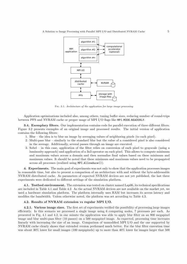
Figure 3.1 presents the most important architecture components and their dependencies. As previouslystated, image files are served by a PFS. An application accesses it using MPI I/O API. The NVRAM cache is atransparent component that improves efficiency of file access. Optionally, an application can use computationalaccelerators.
3.3. Performance optimization. According to the description of the NVRAM based cache, overheadfor opening and closing a file may have a significant impact on application execution time. In a typical HPCcase this issue is negligible – in long running applications the gain from faster data access fully compensates theinitialization and deinitialization phases. However, omitting this overhead for fast and simple image processingalgorithms would be noticeable. The proposed application is prepared to be used as a service that is able toprocess requested images one by one. The common idea in HPC used for avoidance of waiting for a data isoverlapping communication and computation. In our application we implemented a similar approach – imageprocessing overlaps with opening/closing a file.
Another important task was tuning the PFS. Our cluster was equipped both with Infiniband and 10Gb/sEthernet, so we were able to separate the application and the PFS traffic. Internal MPI communication wasbased on Infiniband, while our cache was connected to PFS using Ethernet. The OrangeFS setting that hasthe most impact on significant reduction of application execution time was turning off TroveSyncData option.It allowed to omit costly data synchronization after each operation at the cost of increased risk of loosing data.Instead of protection offered by OrangeFS we can use the fail-safe mode built into the NVRAM cache mechanismor take the risk – in the worst case the application will process a lost image once more.
1http://mvapich.cse.ohio-state.edu/
A Solution to Image Processing with Parallel MPI I/O and Distributed NVRAM Cache 5
Fig. 3.1. Architecture of the application for large image processing
Application optimizations included also, among others, tuning buffer sizes, reducing number of round-tripsbetween PFS and NVRAM cache or proper usage of MPI I/O flags like MPI MODE READONLY.
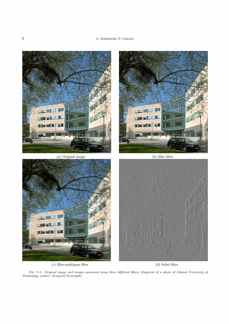
3.4. Exemplary filters. Our implementation contains code for parallel execution of three different filters.Figure 3.2 presents exemples of an original image and processed results. The initial version of applicationcontains the following filters:
1. Blur – the idea is to blur an image by averaging values of neighboring pixels (to each pixel).2. Multi-pass blur – similarly to the standard blur but the value of a considered pixel is also considered
in the average. Additionally, several passes through an image are executed.3. Sobel – in this case, application of the filter relies on conversion of each pixel to grayscale (using a
luminosity approach) and application of a 3x3 operator on each pixel. This allows to compute minimumand maximum values across a domain and then normalize final values based on these minimum andmaximum values. It should be noted that these minimum and maximum values need to be propagatedacross all processes (realized using MPI Allreduce()).
4. Experiments. The main goal of experiments was not only to show that the application processes imagesin reasonable time, but also to present a comparison of an architecture with and without the byte-addressableNVRAM distributed cache. As parameters of expected NVRAM devices are not yet published, the last threeexperiments were dedicated to different settings of the simulation platform.
4.1. Testbed environment. The extension was tested on cluster named Lap06, its technical specificationsare included in Table 4.1 and Table 4.2. As the actual NVRAM devices are not available on the market yet, weused a hardware simulation platform. The platform internally uses RAM but increases its access latency andmodifies the bandwidth. Unless otherwise noted, the platform was set according to Table 4.3.
4.2. Results of NVRAM extension vs regular MPI I/O.
4.2.1. Various image sizes. The first set of experiments verified the possibility of processing large imagesefficiently. In this scenario we processed a single image using 6 computing nodes, 7 processes per each. Aspresented in Fig. 4.1 and 4.2, in one minute the application was able to apply blur filter on an 800 megapixelimage and blur multi-pass filter (10 passes) on a 500 megapixel image. As expected, processing time increaseslinearly with increasing the size of an image. Comparison of unmodified MPI I/O and the one supported byNVRAM cache clearly shows that extended version performed much better. For the blur filter execution timewas about 30% lower for small images (100 megapixels) up to more than 40% lower for images larger that 500
6 A. Malinowski, P. Czarnul
(a) Original image (b) Blur filter
(c) Blur-multipass filter (d) Sobel filter
Fig. 3.2. Original image and images processed using three different filters (fragment of a photo of Gdansk University ofTechnology, author: Krzysztof Krzempek)

A Solution to Image Processing with Parallel MPI I/O and Distributed NVRAM Cache 7
Table 4.1Hardware used in performance tests
Number of computing nodes 6Number of PFS nodes 2CPU 2 x Intel R⃝ Xeon R⃝ E5-4620RAM 15GBNetwork 40Gb/s Infiniband, 10Gb/s EthernetStorage SSDNVRAM simulation 17GB, hardware simulation
Table 4.2Clusters’ software configuration
Operating system CentOS release 6.5MPI implementation MPICH 3.2PFS Orange-FS 2.9.6
Table 4.3NVRAM simulation platform parameters
additional latency before accessing the data 2000nsadditional latency before flushing the data on device 600nsmemory bandwidth divider 4
megapixels. According to previous expectations, less demanding algorithms like blur suffer from overhead foropening and closing a file. This issue does not occur with blur multi-pass – for this scenario we were able toobserve more than 90% reduction of the execution time.
Fig. 4.1. Image processing results, blur filter, 6 nodes, 42 processes, 512kB application buffers
4.2.2. Various number of images. The next set of tests was focused on testing effectiveness of overlap-ping image processing with opening/closing a file. In order to verify the approach we compared the proposedapplication running with multiple files and the same application, but executed for each single image sequentially.Results presented in Fig. 4.3 and 4.4 demonstrate reduced execution times for application with overlapping.

8 A. Malinowski, P. Czarnul
Fig. 4.2. Image processing results, blur multi-pass filter, 6 nodes, 42 processes, 512kB application buffers
Unfortunately, the gain from implementation of overlapping was lower that expected. For a relatively simplefilter – Sobel – we observed reduction of execution time at the level of 5%. More complicated algorithms likeblur multi-pass allow for saving more time – for test scenario illustrated in Fig. 4.4 it was about 10%.
Fig. 4.3. Image processing results, Sobel filter, 6 nodes, 42 processes, 512kB application buffer, each image of 1 gigapixel
4.2.3. Various buffer sizes. Although our NVRAM distributed cache is designed to work well withsmall data chunks (even with access to single bytes), the proposed application uses internal buffers. Two bufferslocated in RAM, one for read and one for write operations, prevent from too frequent file requests. Resultspresented in Fig. 4.5 and 4.6 prove that the NVRAM cache is prepared for serving even small data chunks.

A Solution to Image Processing with Parallel MPI I/O and Distributed NVRAM Cache 9
Fig. 4.4. Image processing results, blur multi-pass filter, 6 nodes, 42 processes, 512kB application buffer, each image of1 gigapixel
Results were similar both for simple and more demanding processing algorithms. With unmodified MPI I/O andrequests lower than 128kB the application is extremely slow, because the PFS is flooded with a large numberof requests incoming frequently. In our opinion, such a result is another argument for applying the proposedarchitecture – implementing buffers is an additional overhead for developers, especially for more complicated,non-linear image processing algorithms. The proposed solution allows to focus more on implementing algorithmsthemselves, rather than on difficult I/O optimization.
Fig. 4.5. Image processing results, Sobel filter, 6 nodes, 42 processes, image of 0.5 gigapixel

10 A. Malinowski, P. Czarnul
Fig. 4.6. Image processing results, blur filter, 6 nodes, 42 processes, image of 0.5 gigapixel
4.2.4. Scalability. One of the most important parameters of HPC applications is scalability regarded asthe potential of reducing execution time with increasing hardware resources, today most often the number ofa cluster nodes and consequently the number of CPUs and cores. It may seem that with processing multipleimages, the application does not require good scalability because it could be executed multiple times for eachimage independently. In practice, when the I/O is the bottleneck of the system, running many instances of adata intensive application may result in overloading of PFS.
Figure 4.7 shows application speedup while increasing the number of nodes. Unmodified MPI I/O doesnot scale well because the gain from higher computational power of greater number of nodes is insignificantwhen PFS is more and more overloaded. The speedup of execution with NVRAM cache is also far fromlinear, but still significant. Scalability is of the features of the distributed architecture of NVRAM cache. Thesolution is designed in such way that each node participates in serving read/write requests. With an increasingnumber of a file accesses from a higher number of processes, the extension has more nodes to process it, so theaverage number of requests per node is constant. Furthermore, better scalability results are expected for moredemanding algorithms with a higher ratio of computations to I/O.
4.2.5. Various NVRAM simulation parameters. As we do not have NVRAM based devices yet, weused a hardware simulation platform. Unknown properties of final devices result in necessity for testing solutionsfor many different configurations in the range of expected parameter values. Although NVRAM devices shouldoutperform today’s SSDs, we assumed pessimistic values at the level similar to announced SSD specifications(i.e. Intel R⃝ Optane R⃝ P4800X with typical latency of less than 10µs, up to 2400/2000MB/s read/write speedand 500k IOPS for random requests [3]). The following three tests were performed using the blur multi-passfilter.
Figure 4.8 presents comparison of execution times according to the memory bandwidth. Our nodes wereequipped with DDR3 1600Mhz memory units, the simulator allowed to divide the bandwidth by a certain factor.In the plot we can observe that this parameter does not have a significant impact on the proposed application– average growth of the execution time after reducing the bandwidth was less than 2.6%. With frequent, lowsize requests our application depends more on the access latency rather than bandwidth.
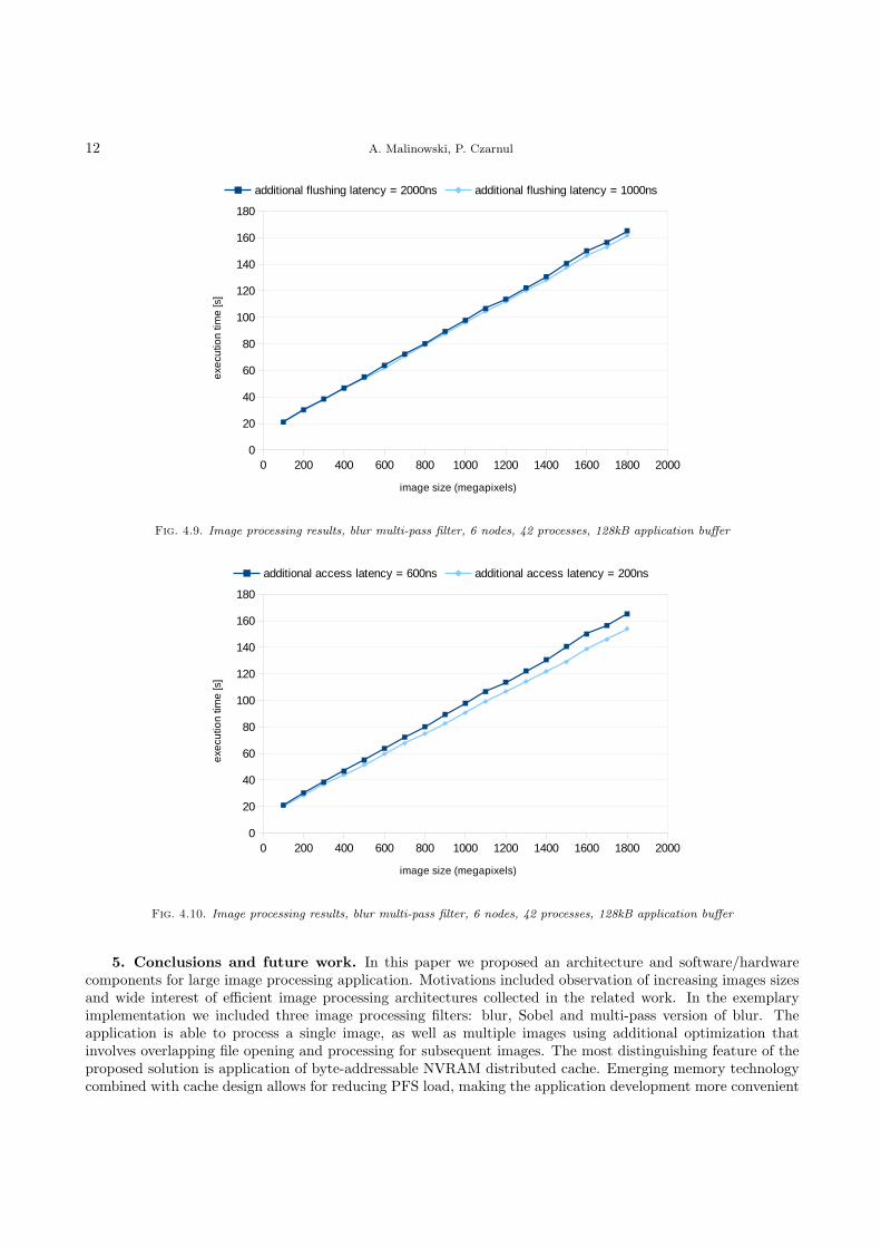
Results shown in Fig. 4.9 concern an additional delay required to flush the cached data onto the deviceto make it persistent. The plot is quite similar to the previous one – even when the additional latency beforeflushing the data was doubled, average execution time of the application grew up about 2%. This latency is

A Solution to Image Processing with Parallel MPI I/O and Distributed NVRAM Cache 11
Fig. 4.7. Image processing results, blur multi-pass filter, 512kB application buffers, image of 1.5 gigapixel
Fig. 4.8. Image processing results, blur multi-pass filter, 6 nodes, 42 processes, 128kB application buffer
added only for write accesses and in our application write operations are less common than reads.
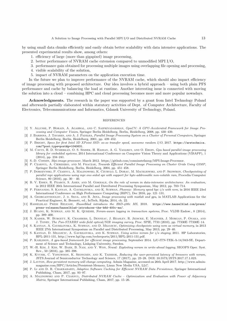
A much more visible impact on execution time is shown in Fig. 4.10. In this scenario we increased theadditional latency added for each memory request. Obtained results resulted in about 7% growth of processingtime.
Those three experiments proved that the impact of NVRAM parameters is significant in terms of executiontime, but insignificant when comparing the application with NVRAM cache and the one without. This leadsto the conclusion that if only NVRAM devices provide performance at the level of SSD devices or better, theproposed architecture will be more efficient using the proposed distributed cache.
12 A. Malinowski, P. Czarnul
Fig. 4.9. Image processing results, blur multi-pass filter, 6 nodes, 42 processes, 128kB application buffer
Fig. 4.10. Image processing results, blur multi-pass filter, 6 nodes, 42 processes, 128kB application buffer
5. Conclusions and future work. In this paper we proposed an architecture and software/hardwarecomponents for large image processing application. Motivations included observation of increasing images sizesand wide interest of efficient image processing architectures collected in the related work. In the exemplaryimplementation we included three image processing filters: blur, Sobel and multi-pass version of blur. Theapplication is able to process a single image, as well as multiple images using additional optimization thatinvolves overlapping file opening and processing for subsequent images. The most distinguishing feature of theproposed solution is application of byte-addressable NVRAM distributed cache. Emerging memory technologycombined with cache design allows for reducing PFS load, making the application development more convenient
A Solution to Image Processing with Parallel MPI I/O and Distributed NVRAM Cache 13
by using small data chunks efficiently and easily obtain better scalability with data intensive applications. Thepresented experimental results show, among others:
1. efficiency of large (more than gigapixel) image processing,2. better performance of NVRAM cache extension compared to unmodified MPI I/O,3. performance gain obtained for processing multiple images using overlapping file opening and processing,4. visible scalability of the solution,5. impact of NVRAM parameters on the application execution time.
In the future we plan to improve performance of the NVRAM cache, which should also impact efficiencyof image processing with proposed architecture. Our idea involves a hybrid approach – using both plain PFSperformance and cache by balancing the load at runtime. Another interesting issue is connected with movingthe solution into a cloud – combining HPC and cloud processing becomes more and more popular nowadays.
Acknowledgments. The research in the paper was supported by a grant from Intel Technology Polandand afterwards partially elaborated within statutory activities of Dept. of Computer Architecture, Faculty ofElectronics, Telecommunications and Informatics, Gdansk University of Technology, Poland.
REFERENCES
[1] Y. Allusse, P. Horain, A. Agarwal, and C. Saipriyadarshan, GpuCV: A GPU-Accelerated Framework for Image Pro-cessing and Computer Vision, Springer Berlin Heidelberg, Berlin, Heidelberg, 2008, pp. 430–439.
[2] J. Barbosa, J. Tavares, and A. J. Padilha, Parallel Image Processing System on a Cluster of Personal Computers, SpringerBerlin Heidelberg, Berlin, Heidelberg, 2001, pp. 439–452.
[3] P. Bright, Specs for first Intel 3D XPoint SSD: so-so transfer speed, awesome random I/O, 2017. https://arstechnica.
com/?post type=post&p=1040631.[4] M. Cavus, H. D. Sumerkan, O. S. Simsek, H. Hassan, A. G. Yaglikci, and O. Ergin, Gpu based parallel image processing
library for embedded systems, 2014 International Conference on Computer Vision Theory and Applications (VISAPP), 1(2014), pp. 234–241.
[5] S.-D. Cosmin, Mpi-image-processor, March 2012. https://github.com/cosminstefanxp/MPI-Image-Processor.[6] P. Czarnul, A. Ciereszko, and M. Fraczak, Towards Efficient Parallel Image Processing on Cluster Grids Using GIMP,
Springer Berlin Heidelberg, Berlin, Heidelberg, 2004, pp. 451–458.[7] P. Dorozynski, P. Czarnul, A. Malinowski, K. Czurylo, L. Dorau, M. Maciejewski, and P. Skowron, Checkpointing of
parallel mpi applications using mpi one-sided api with support for byte-addressable non-volatile ram, Procedia ComputerScience, 80 (2016), pp. 30 – 40.
[8] B. V. Essen, R. Pearce, S. Ames, and M. Gokhale, On the role of nvram in data-intensive architectures: An evaluation,in 2012 IEEE 26th International Parallel and Distributed Processing Symposium, May 2012, pp. 703–714.
[9] P. Fernando, S. Kannan, A. Gavrilovska, and K. Schwan, Phoenix: Memory speed hpc i/o with nvm, in 2016 IEEE 23rdInternational Conference on High Performance Computing (HiPC), Dec 2016, pp. 121–131.
[10] A. Georgantzoglou, J. d. Silva, and R. Jena, Image processing with matlab and gpu, in MATLAB Applications for thePractical Engineer, K. Bennett, ed., InTech, Rijeka, 2014, ch. 22.
[11] Hasselblad Press Release, Hasselblad introduces the H6D-400c MS, 2018. https://www.hasselblad.com/press/
press-releases/hasselblad-introduces-the-h6d-400c-ms/.[12] J. Huang, K. Schwan, and M. K. Qureshi, Nvram-aware logging in transaction systems, Proc. VLDB Endow., 8 (2014),
pp. 389–400.[13] N. Kaiser, W. Burgett, K. Chambers, L. Denneau, J. Heasley, R. Jedicke, E. Magnier, J. Morgan, P. Onaka, and
J. Tonry, The Pan-STARRS wide-field optical/NIR imaging survey, Proc. SPIE, 7733 (2010), pp. 77330E–77330E–14.[14] S. Kannan, A. Gavrilovska, K. Schwan, and D. Milojicic, Optimizing checkpoints using nvm as virtual memory, in 2013
IEEE 27th International Symposium on Parallel and Distributed Processing, May 2013, pp. 29–40.[15] S. Kannan, D. Milojicic, A. Gavrilovska, and K. Schwan, Using active nvram for i/o staging, 2011. HP Laboratories,
HPL-2011-131, http://www.hpl.hp.com/techreports/2011/HPL-2011-131.pdf.[16] P. Karlsson, A gpu-based framework for efficient image processing, September 2014. LiU-ITN-TEK-A-14/043-SE, Depart-
ment of Science and Technology, Linkping University, Sweden.[17] W.-H. Kim, J. Kim, W. Baek, B. Nam, and Y. Won, Nvwal: Exploiting nvram in write-ahead logging, SIGOPS Oper. Syst.
Rev., 50 (2016), pp. 385–398.[18] K. Kyusik, C. Yongwoon, K. Seongmin, and K. Taeseok, Reducing the user-perceived latency of browsers with nvram,
JSTS:Journal of Semiconductor Technology and Science, 17 (2017), pp. 23–28. DOI: 10.5573/JSTS.2017.17.1.023.[19] J. Layton, How persistent memory will change computing. Admin Magazine, accessed on 26th April 2017. http://www.admin-
magazine.com/HPC/Articles/Persistent-Memory, Linux New Media USA, LLC.[20] P. Li and D. R. Chakrabarti, Adaptive Software Caching for Efficient NVRAM Data Persistence, Springer International
Publishing, Cham, 2017, pp. 93–97.[21] A. Malinowski and P. Czarnul, Distributed NVRAM Cache – Optimization and Evaluation with Power of Adjacency
Matrix, Springer International Publishing, Cham, 2017, pp. 15–26.

14 A. Malinowski, P. Czarnul
[22] A. Malinowski, P. Czarnul, K. Czury lo, M. Maciejewski, and P. Skowron, Multi-agent large-scale parallel crowdsimulation, Procedia Computer Science, 108 (2017), pp. 917 – 926. International Conference on Computational Science,ICCS 2017, 12-14 June 2017, Zurich, Switzerland.
[23] A. Malinowski, P. Czarnul, P. Dorozynski, K. Czury lo, L. Dorau, M. Maciejewski, and P. Skowron, A Parallel MPII/O Solution Supported by Byte-addressable Non-volatile RAM Distributed Cache, in Position Papers of the 2016 Feder-ated Conference on Computer Science and Information Systems, vol. 9 of Annals of Computer Science and InformationSystems, PTI, 2016, pp. 133–140.
[24] A. Malinowski, P. Czarnul, M. Maciejewski, and P. Skowron, A Fail-Safe NVRAM Based Mechanism for EfficientCreation and Recovery of Data Copies in Parallel MPI Applications, in Information Systems Architecture and Technology:Proceedings of 37th International Conference on Information Systems Architecture and Technology – ISAT 2016 – PartII, Springer International Publishing, 2017, pp. 137–147.
[25] A. Mochizuki, N. Yube, and T. Hanyu, Design of a computational nonvolatile ram for a greedy energy-efficient vlsiprocessor, in IECON 2015 - 41st Annual Conference of the IEEE Industrial Electronics Society, Nov 2015, pp. 003283–003288.
[26] NASA, Space Shuttle Mission STS-48 Press Kit, 1991. https://science.ksc.nasa.gov/shuttle/missions/sts-48/
sts-48-press-kit.txt.[27] NASA/ESA, Hubbles High-Definition Panoramic View of the Andromeda Galaxy, 2015. http://www.spacetelescope.org/
images/heic1502a/.[28] C. Nicolescu and P. Jonker, Parallel low-level image processing on a distributed-memory system, Springer Berlin Heidel-
berg, Berlin, Heidelberg, 2000, pp. 226–233.[29] C. Nicolescu and P. Jonker, A data and task parallel image processing environment, Parallel Computing, 28 (2002), pp. 945
– 965.[30] A. Ozdemir and T. Altilar, Gpu based parallel image processing for plant growth analysis, in 2014 The Third International
Conference on Agro-Geoinformatics, Aug 2014, pp. 1–6.[31] A. Remnyi, S. Sznsi, I. Bndi, Z. Vmossy, G. Valcz, P. Bogdanov, S. Sergyn, and M. Kozlovszky, Parallel biomedical
image processing with gpgpus in cancer research, in 3rd IEEE International Symposium on Logistics and IndustrialInformatics, Aug 2011, pp. 245–248.
[32] W. Ruyten and W. E. Sisson, Message passing for parallel processing of pressure-sensitive paint images, in Users GroupConference (DOD UGC’04), 2004, June 2004, pp. 308–312.
[33] J. M. Squyres, A. Lumsdaine, and R. L. Stevenson, A toolkit for parallel image processing, in SPIE Annual Meeting, SanDiego, 1998.
[34] R. Thakur, W. Gropp, and E. Lusk, Data sieving and collective I/O in romio, Frontiers ’99 - Seventh Symposium OnFrontiers Massively Parallel Computation, Proc., (1999), pp. 182–189.
[35] K. Vincent, D. Nguyen, B. Walker, T. Lu, and T.-H. Chao, Gpu processing for parallel image processing and real-timeobject recognition, 2014.
[36] M. Wasi-ur Rahman, N. S. Islam, X. Lu, and D. K. D. Panda, Can non-volatile memory benefit mapreduce applications onhpc clusters?, in Proceedings of the 1st Joint International Workshop on Parallel Data Storage & Data Intensive ScalableComputing Systems, PDSW-DISCS ’16, Piscataway, NJ, USA, 2016, IEEE Press, pp. 19–24.
[37] H. Yu, Y. Wang, S. Chen, W. Fei, C. Weng, J. Zhao, and Z. Wei, Energy efficient in-memory machine learning for dataintensive image-processing by non-volatile domain-wall memory, in 2014 19th Asia and South Pacific Design AutomationConference (ASP-DAC), Jan 2014, pp. 191–196.
[38] M. Zhang, Bentley Used NASA Tech to Create This 53-Gigapixel Car Photo, 2016. PetaPixel, https://petapixel.com/2016/06/23/bentley-used-nasa-tech-create-53-gigapixel-photo-car/.
[39] Y. Zhang, J. Yang, A. Memaripour, and S. Swanson, Mojim: A reliable and highly-available non-volatile memory system,in Proceedings of the Twentieth International Conference on Architectural Support for Programming Languages andOperating Systems, ASPLOS ’15, New York, NY, USA, 2015, ACM, pp. 3–18.
Edited by: Dana PetcuReceived: Nov 6, 2017Accepted: Dec 23, 2017
Scalable Computing: Practice and Experience
Volume 19, Number 1, pp. 15–29. http://www.scpe.org
DOI 10.12694/scpe.v19i1.1390ISSN 1895-1767c⃝ 2018 SCPE
SCALE-EA: A SCALABILITY AWARE PERFORMANCE TUNING FRAMEWORK FOR
OPENMP APPLICATIONS
SHAJULIN BENEDICT∗
Abstract. HPC application developers, including OpenMP-based application developers, have stepped forward to endeavor thefuture design trends of exa-scale machines, such as, increased number of threads/cores, heterogeneous architectures, multiple levelsof memories, and so forth; and, they have initiated procedures to address application level challenges, such as, data-driven scalabilityissues, energy consumption requirements, data availability needs, and so forth. Despite the existence of manual performance tuningsolutions, users still deem it to be an intricate process. This paper proposes a scalability aware autotuning framework (SCALE-EA) that automatically identifies an efficient number of threads for OpenMP parallel regions using a Firefly Algorithm (FA) and anewly designed Modeling Assisted Firefly Algorithm (MAFA). MAFA of SCALE-EA was implemented in two approaches: ModelingAssisted Firefly Algorithm with Random Forest Modeling support (MAFA-RFM) and Modeling Assisted Firefly Algorithm withLinear Regression Modeling support (MAFA-LRM). The modeling and prediction algorithms of the proposed MAFA of SCALE-EAwere based on the execution time and the hardware performance events of code regions of OpenMP applications. Experiments wereconducted on two machines, namely, a Haswell based machine and an AMD Opteron based 48 core machine. The experimentalresults of the MAFA of SCALE-EA manifested the energy efficiencies of 31.21 to 77.3 percentage and the search time efficienciesof 5.53 to 32.56 percentage for candidate OpenMP applications such as CoMD, Arraybench, Taskbench, and Syncbench.
Key words: Auto Tuning, OpenMP Applications, Modeling and Scalability
AMS subject classifications. 68M20, 68W10
1. Introduction. High Performance Computing (HPC) application developments are invariably croppingup among various scientific domains, such as, High Energy Physics (HEP), bioinformatics, eyewear computing,visualizations, electronic automation, graph-based machine learning, and so forth. OpenMP based programmingmodel is indeed reaching out to become a prominent programming model among a sector of HPC applicationdevelopers owing to the adequate doctrine of standards (OpenMP 4.0 and 4.5), ease of use, controlled program-ming support, smooth applicability to programmers belonging to various scientific disciplines, and due to thenotion of having millions of cores in future exascale machines.
However, the realization of efficiently utilizing HPC applications in its present form for future large scalemachines requires innovative approaches to mitigate the following possible risky scenarios:
1. the performance of applications becomes more sensitive to data movement, data availability, data prove-nance, data management policies, and so forth – a future software-cum-hardware computing systemmust consider the massive storage options of machines, resiliency nature of applications, dynamic com-puting behavior of applications, and the dynamic nature of the data access patterns of applications (bigdata).
2. the current implementations of OpenMP applications might not have considered the design aspects ofemerging memory models (including data persistence of modern memory architectures), infrastructuralimprovements, future parallel data structures, and so forth.
3. the scalability of applications might get an impoverished lead as applications are usually not portedand tested for scalable machines.
4. the energy efficiency of applications could exhibit a daunting scenario when executed on machines withvarying degrees of parallelism – smaller or larger.
5. the current OpenMP application developers might not have quantified the possible uncertainties thatmight evolve due to the underlying future parallel software frameworks.
In short, to mitigate these challenges, programmers or developers have to diligently write scalable andenergy efficient parallel algorithms by employing the apt scalability features of programming languages and byconsidering the underlying requirements of machines. Vividly, OpenMP based application programmers haveto gain sophisticated knowledge on handling the newer OpenMP constructs in order to attain higher scalability,portability, and energy efficiency – for instances, the synchronization points of OpenMP applications, such as,
∗Indian Institute of Information Technology Kottayam, Kerala, India - 695016. ([email protected]) – Formerly theGuest Professor of Technical University Munich, Germany.
15

16 S. Benedict
OpenMP barrier constructs should be limited or enriched; the granularity of OpenMP parallel regions shouldbe optimized to achieve higher scalability; and, the programmers should efficiently utilize the OpenMP privatedata clauses in an application.
In general, the non-scalable and the energy/performance inefficient code regions of an application can beidentified and manually tuned. However, the manual tuning processes might laid down hefty responsibilities tousers – an intricate process. One solution that makes sense and intends to work in large scale HPC scenarios is toestablish an autotuning tool or a framework that automatically finds the non-scalable or energy inefficient partsof the code regions of applications and tunes them accordingly. Historically, a notion of framing autonomiccomputing systems was highly appreciated by researchers for decades [11, 29]. Moreover, researchers hadshown their keen interest in counteracting the scalability and the energy consumption issues of applications[2, 4, 15, 31] at various levels of computing systems so that the existing applications could be executed on futuremachines at ease.
Auto tuning, although a promising solution for tuning HPC applications, easily leads to voluminous com-binations of optimization options which might impede the search time of the tuning process. In addition, theautotuning process could inundate the search space with an immense volume of performance data, as autotuningsystems are, in general, self-aware, self-configurable [42], context-aware, and self-optimizable systems. In mostcases, the autotuning systems are guided in a single-objective or in a multi-objective modes of operations basedon pre-defined objectives, such as, minimizing energy consumption of code regions of applications, maximizingthe utilization of machines, minimizing the data movement to Dynamic Random Access Memory (DRAM), andso forth. Thus, there is an increasing need for autotuning solutions or frameworks that intelligently minimizesthe search time of the tuning processes.
This paper proposes the SCALE-EA framework, a Scalability-Aware performance tuning framework usingEnergyAnalyzer (EA), for OpenMP applications – EnergyAnalyzer tool is an online based energy consumptionanalysis tool for HPC applications. SCALE-EA automatically identifies the efficient number of threads forindividual parallel regions of OpenMP applications using FA and MAFA. The proposed FA and MAFA ofSCALE-EA improved the search time of the tuning process and enhanced the energy efficiency of applications.The proposed method was evaluated using several OpenMP applications / benchmarks, such as, CoMD fromthe co-design center of LLNL, USA [14], and OpenMP benchmarks from EPCC [17], on a Haswell processorbased HP-Zbook-15G machine and a 48 core HPProliant machine.
In succinct, the paper has the following contributions:
1. an SCALE-EA framework for automatically finding an efficient number of threads for the parallelregions of OpenMP applications was proposed.
2. FA and modeling assisted heuristic algorithms were implemented in SCALE-EA in order to reduce thesearch time of the tuning process. The modeling assisted heuristic algorithms were implemented intwo flavors: a) Modeling Assisted Firefly Algorithm using Linear Regression Modeling (MAFA-LRM)and b) Modeling Assisted Firefly Algorithm using Random Forest Modeling (MAFA-RFM). MAFAalgorithms are the modified versions of FA.
3. Experimental evaluations of the proposed SCALE-EA and its associated algorithms were carried outusing OpenMP applications, such as, Arraybench, Syncbench, Taskbench, and CoMD applications.
The rest of the paper is organized as follows. Section 2 presents existing autotuning frameworks andtheir solutions. Section 3 explains the proposed scalability-aware performance tuning framework for OpenMPapplications and Section 4 discusses the modified firefly algorithm which adds modeling support towards thesearch process. Section 5 manifests the proposed mechanism called the SCALE-EA framework. And, finally,Section 6 presents conclusions.
2. Related Works. HPC applications, specifically data-driven applications, are increasing in the scientificmarket from various scientific disciplines, such as, massive graphs, HEP, bioinformatics, healthcare, distributedmanufacturing, electronic automation, visualization applications (social networks), multi-physics simulations,and so forth. In the meantime, technological advances in hardware architectures are nearing exascale speedthrough co-design architectural designs, abundant General Purpose Graphical Processing Units (GPGPUs),hierarchical clustering of heterogeneous machines, and so forth. Despite the growth seen in the applicationsector and in the hardware architectural design sector of HPC, the performances of applications, including the

SCALE-EA: A Scalability Aware Performance Tuning Framework for OpenMP Applications 17
Fig. 3.1. SCALE-EA: Scalability Aware Performance AutoTuning Framework for OpenMP Applications
scalability and the energy efficiency of applications, should be concerned about by the researchers.
The HPC community, therefore, oriented their mindset to mitigate the effects of known performance issuesof large scale systems such as the dynamic nature of big data in applications (data sizes), heterogeneous hardwarearchitectures [7], energy consumption issues, scalability issues [22, 39], uncertainty of resources (including dataresources), and so forth [18].
In fact, the energy consumption issues of HPC applications should be addressed due to the scarcity of powersources (especially in the developing countries, such as, India), owing to the emission of carbon footprints [10]which lead to environmental hazards, and, due to the emerging power wall problem of dark silicons [31].
There exists a few standalone energy reduction mechanisms for HPC applications [28, 36, 21]. The most ofthe existing approaches are either manual [34] or application-centric.
Researchers have proposed autotuning frameworks/solutions [16, 23, 24, 25, 13] in order to achieve per-formance/energy improvements. Studies have also led a subset of researchers to frame autotuning solutionsat compile time [2, 9, 12, 27, 32] and a few others at run time of applications [37, 3, 40, 8]. In addition,a few autotuning solutions with more emphasis to IOs were designed in [5]. To improve the performance ofheterogeneous systems and applications, the authors of [6] have designed an autotuning solution. Additionally,tool developers are constantly finding mechanisms to assist application developers in terms of automaticallyimproving the performance efficiency of HPC applications.
To avoid the burdens caused due to the search time and the emergence of abundant performance data, afew researchers have utilized modeling mechanisms [26, 1] to forecast the performance issues of applicationsand to tune applications. In addition, modeling assisted automated systems have been successful in cloud anddistributed environments [30]. Recently, researchers have adopted autotuning using Domain Specific Languagesfor autotuning applications in ANTAREX project [13].
This paper proposed a combination of heuristics and modeling approach for the tuning process of OpenMPbased HPC applications. To do so, Firefly Algorithm (FA), a heuristic method, is modified with modelingalgorithms, such as, RFM and LRM, in this paper. A detailed description about the proposed SCALE-EAframework based on FA and MAFA algorithms is discussed in Section 3.
3. Scalability Aware AutoTuning using EnergyAnalyzer (SCALE-EA). SCALE-EA frameworkdoes scalability aware performance autotuning of OpenMP applications. The framework is built based onEnergyAnalyzer tool, an online based energy consumption analysis tool. This section explains the SCALE-EAframework and the entities involved in pursuing the performance aware autotuning mechanism for OpenMPapplications.

18 S. Benedict
3.1. SCALE-EA Framework Functionalities. The functionalities of the proposed SCALE-EA frame-work, the extensions made towards EnergyAnalyzer tool, are described as follows:
SSTranslator and its Extension. SSTranslator, an entity of EnergyAnalyzer tool, is extended to support theproposed SCALE-EA framework. It is a source-to-source translator which includes program statements, suchas,
#pragma start_user_region
---
#pragma end_user_region
These statements notify the Monitoring Manager entity of EnergyAnalyzer about the user-specified code re-gions of applications. The performance / energy consumption values of these user-specified regions are measuredusing the Monitoring Manager entity of EnergyAnalyzer at the runtime of applications.
The extended version of SSTranslator additionally identifies each parallel regions of OpenMP based appli-cations. These parallel regions are marked with two additional statements, such as,
omp_set_dynamic(0);
omp_set_num_threads(SCALEEA_NUM_THREADS_filename_n);
where n resembles the unique number for each omp parallel regions in an application and filename is thefilename representation of applications.
The line omp set dynamic(0) is automatically added before the omp parallel regions of OpenMP-basedapplications using the extended version of SSTranslator. This statement instructs compilers to disable dynamicallocation of threads. The variable SCALEEA NUM THREADS filename n is automatically defined at the initialstage of the file using #ifdef conditions of C/C++ definitions. This is mandatory for the proposed SCALE-EA framework as the framework would later assign the number of threads for each omp parallel regions. Theheuristics of SCALE-EA are responsible for assigning the values to these variables.
In addition, the line numbers for omp parallel regions and the file names of applications where the regionsbelong to are noticed in a separate .sst file (static source-to-source file) of the SCALE-EA framework.
Performance/Energy Measurements. After inserting the required statements for SCALE-EA, (for instances,the statements which would disable the dynamic allocation of threads to OpenMP applications and enable per-formance measurements), the application is compiled with the MMLibrary of EnergyAnalyzer. The MMLibraryof EnergyAnalyzer measures the performance values of the user-specified code regions of applications and storesthe performance values in EAPerfDB, a no-sql (Mongodb) based performance database of EnergyAnalyzer tool.
Heuristic Support. Selecting efficient numbers of threads for each omp parallel regions of OpenMP appli-cation is a time consuming task. Thus, SCALE-EA framework depends on heuristics which suggest efficientnumbers of threads for each omp parallel regions.
In this paper, Firefly Algorithm (FA) is applied in the SCALE-EA framework in order to find the efficientnumber of threads for OpenMP applications. In addition, the time spent for finding the efficient number ofthreads (the search time) is further reduced using the modified versions of FA – MAFA-RFM and MAFA-LRM.Detailed discussions on the Firefly Algorithm (FA) and MAFA can be found in Section 4.
4. FA and MAFA of SCALE-EA. In this paper, FA and a modified version of FA, namely, ModelingAssisted Firefly Algorithm (MAFA) are proposed for identifying an efficient number of threads for OpenMPapplications. MAFA is implemented in two approaches, namely, MAFA-RFM and MAFA-LRM. This sectiondescribes the FA and MAFA in detail.
4.1. Firefly Algorithm (FA). Firefly Algorithm (FA) is a meta-heuristic algorithm which is activelyutilized by a few researchers [41, 19, 35] in order to solve their real-world combinatorial optimizations problems.FA was developed in 2007 by Xin-She Yang at Cambridge University [41]. In fact, the idea of meta-heuristicsintrigued the real world problem solvers when compared to the classical optimization techniques for decadesowing to the algorithms’ problem independent nature – the classical optimization techniques find solutions basedon analytical models (continuous or differentiable functions).
FA, an iterative based heuristic technique or a population based meta-heuristics, was introduced in severalflavors, such as, adaptive, multi-objective, hybrid, DiscreteFA, and so forth. A wide survey of FA and its
SCALE-EA: A Scalability Aware Performance Tuning Framework for OpenMP Applications 19
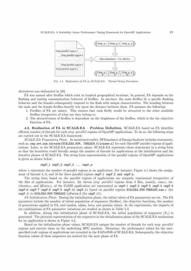
Fig. 4.1. Realization of FA in SCALE-EA – Thread String Formation
derivatives was elaborated in [20].FA was named after fireflies which exist in tropical geographical locations. In general, FA depends on the
flashing and mating communication behavior of fireflies. In succinct, the male fireflies lit a specific flashingbehavior and the females subsequently respond to the flash with unique characteristics. The bonding betweenthe male and the female fireflies heavily rely upon the distance between them. FA assumes the following:
1. Fireflies of FA are unisex. This ensures that each firefly would be attracted to the other availablefireflies irrespective of what sex they belong to.
2. The attractiveness of fireflies is dependent on the brightness of the fireflies, which is the the objectivefunction of FA.
4.2. Realization of FA in SCALE-EA – Problem Definition. SCALE-EA based on FA identifiesefficient number of threads for each omp parallel regions of OpenMP applications. To do so, the following stepsare carried out in the SCALE-EA framework:
SCALE-EA Preparatory Phase. As mentioned earlier, SSTranslator of EnergyAnalyzer includes statements,such as, omp set num threads(SCALEEA NUM THREADS filename n) for each OpenMP parallel regions of appli-cations. Later, in the SCALE-EA preparatory phase, SCALE-EA represents those statements in a string formso that the heuristics could literally assign the number of threads for applications at the initialization and theiterative phases of SCALE-EA. The string form representation of the parallel regions of OpenMP applicationsis given as shown below:
ompP_1 ompP_2 ompP_3 ... ompP_n
where n represents the number of parallel regions in an application. For instance, Figure 4.1 shows the assign-ment of threads 4, 8, and 16 for three parallel regions ompP 1 ompP 2 and ompP n.
The string form based on the parallel regions of applications are uniquely represented irrespective ofthe files of applications. For instance, the eleven omp parallel regions from 3 files, namely, eam.c, ini-tAtoms.c, and ljForce.c, of the CoMD application are represented as ompP 1 ompP 2 ompP 3 ompP 4 ompP 5
ompP 6 ompP 7 ompP 8 ompP 9 ompP 10 ompP 11 based on parallel regions SCALEEA NUM THREADS eam 1 (forompP 1) to SCALEEA NUM THREADS ljForce 2 (for ompP 11).
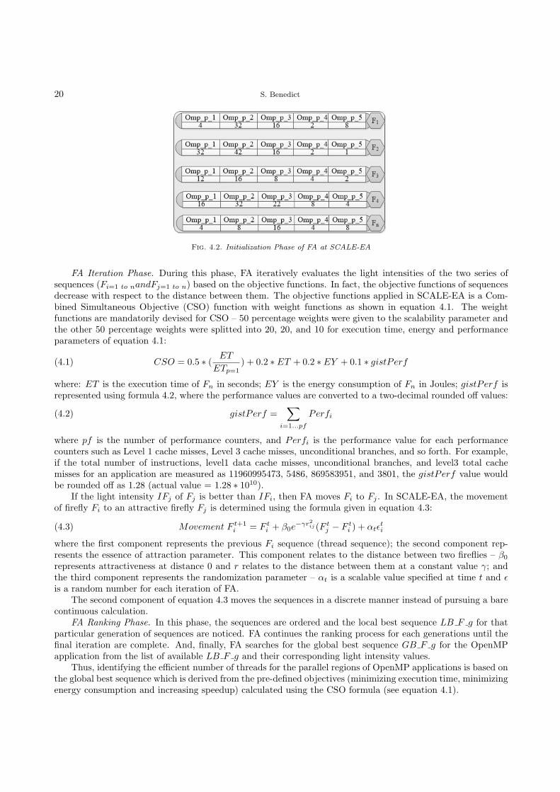
FA Initialization Phase. During the initialization phase, the initial values of FA parameters are set. The FAparamters include the number of initial population of sequences (fireflies), the objective functions, the numberof generations applied in FA, and epsilon, alpha, beta, and gamma values. In the experiments, the impacts ofsix combinations of FA parameter variations are studied as shown in Table 5.3.
In addition, during this initialization phase of SCALE-EA, the initial population of sequences (Fn) isgenerated. The pictorial representation of the sequences in the initialization phase of the SCALE-EA mechanismfor an application is shown in Figure 4.2.
Based on the initialization phase values, SCALE-EA assigns the number of threads for each omp parallel
regions and execute them on the underlying HPC machine. Meantime, the performance values for the user-specified code regions of applications are recorded in the EAPerfDB of SCALE-EA. Subsequently, the objectivefunction values of these sequences are noticed for the next phase of FA.
20 S. Benedict
Fig. 4.2. Initialization Phase of FA at SCALE-EA
FA Iteration Phase. During this phase, FA iteratively evaluates the light intensities of the two series ofsequences (Fi=1 to nandFj=1 to n) based on the objective functions. In fact, the objective functions of sequencesdecrease with respect to the distance between them. The objective functions applied in SCALE-EA is a Com-bined Simultaneous Objective (CSO) function with weight functions as shown in equation 4.1. The weightfunctions are mandatorily devised for CSO – 50 percentage weights were given to the scalability parameter andthe other 50 percentage weights were splitted into 20, 20, and 10 for execution time, energy and performanceparameters of equation 4.1:
CSO = 0.5 ∗ (ET
ETp=1
) + 0.2 ∗ ET + 0.2 ∗ EY + 0.1 ∗ gistPerf(4.1)
where: ET is the execution time of Fn in seconds; EY is the energy consumption of Fn in Joules; gistPerf isrepresented using formula 4.2, where the performance values are converted to a two-decimal rounded off values:
gistPerf =∑
i=1...pf
Perfi(4.2)
where pf is the number of performance counters, and Perfi is the performance value for each performancecounters such as Level 1 cache misses, Level 3 cache misses, unconditional branches, and so forth. For example,if the total number of instructions, level1 data cache misses, unconditional branches, and level3 total cachemisses for an application are measured as 11960995473, 5486, 869583951, and 3801, the gistPerf value wouldbe rounded off as 1.28 (actual value = 1.28 ∗ 1010).
If the light intensity IFj of Fj is better than IFi, then FA moves Fi to Fj . In SCALE-EA, the movementof firefly Fi to an attractive firefly Fj is determined using the formula given in equation 4.3:
Movement F t+1
i = F ti + β0e
−γr2ij (F tj − F t
i ) + αtϵti(4.3)
where the first component represents the previous Fi sequence (thread sequence); the second component rep-resents the essence of attraction parameter. This component relates to the distance between two fireflies – β0
represents attractiveness at distance 0 and r relates to the distance between them at a constant value γ; andthe third component represents the randomization parameter – αt is a scalable value specified at time t and ϵ
is a random number for each iteration of FA.The second component of equation 4.3 moves the sequences in a discrete manner instead of pursuing a bare
continuous calculation.FA Ranking Phase. In this phase, the sequences are ordered and the local best sequence LB F g for that
particular generation of sequences are noticed. FA continues the ranking process for each generations until thefinal iteration are complete. And, finally, FA searches for the global best sequence GB F g for the OpenMPapplication from the list of available LB F g and their corresponding light intensity values.
Thus, identifying the efficient number of threads for the parallel regions of OpenMP applications is based onthe global best sequence which is derived from the pre-defined objectives (minimizing execution time, minimizingenergy consumption and increasing speedup) calculated using the CSO formula (see equation 4.1).

SCALE-EA: A Scalability Aware Performance Tuning Framework for OpenMP Applications 21
Fig. 4.3. Modeling Assisted Firefly Algorithm (MAFA)
4.3. Modeling Assisted Firefly Algorithm (MAFA) – a modified FA. Although classical FA wouldreduce the time for searching the efficient number of threads in OpenMP applications, the search time of theSCALE-EA tuning process can further be improved using prediction models. Reducing the search time oftuning process is crucial while pursuing autotuning in large scale machines. For instance, an application with 9OpenMP parallel regions might have 134217728 number of combinations of thread sequences when experimentedwith 8 threads. This could deliberately issue hefty number of performance data for each combinations of threadsequences. SCALE-EA, thus, proposed a Modeling Assisted Firefly Algorithm (MAFA) in order to furtherreduce the search time of the SCALE-EA tuning process.
In MAFA, a few iterative portions of FA are executed and the other remaining iterative portions of FA arepredicted using prediction algorithms, such as, Random Forest Modeling (RFM) and Linear Regression Models(LRM). In the previous works, prediction algorithms were applied for predicting the efficient problem sizes [38]of applications at compile time. In this paper, these prediction algorithms are applied for the first time forassisting the search process of FA based meta-heuristics – i.e., a modified implementation of firefly algorithm.Based on the utility of RFM or LRM, MAFA is represented as MAFA-RFM and MAFA-LRM.
The working principle of MAFA is pictorially represented in flow chart (see Figure 4.3). In general, MAFAassumes the four phases as similar to FA – Preparatory, Initialization, Iteration, and Ranking phases. Duringthe initialization phase of MAFA, the initial parameters of FA are set; initialization population is defined; and,the maximum number of generations for the tests is initialized. Later, MAFA iteratively evaluates sequencesand their corresponding intensities (objective functions) for the pre-assigned number of generations as discussedin Section 3.
The modification adopted to FA resides in the iterative phase of MAFA. During the iteration phase of MAFA,all of the combinations of thread sequences that are suggested by FA are not executed. Thus, instead of executingand evaluating all of the combinations of sequences (the thread sequences of OpenMP applications), some ofthe combinations of thread sequences are executed and the others are predicted using prediction algorithms. Todo so, initially, the sequences are enrolled in the Training-Execute list (see Figure 4.3). This list ensures thatSCALE-EA executes the OpenMP application during the evaluation step of FA. After a few iterations, there aresufficient number of entries in the Training-Execute list (for instance, 100 entries in the Training-Execute list ofSCALE-EA), the next 30 percentage of the population in the FA generation is enrolled in the Testing-Predictlist of SCALE-EA.
If the sequence is listed in the Testing-Predict list of SCALE-EA, the OpenMP application with the corre-sponding thread sequence would not be compiled or executed in the underlying machine. Rather, the modeling-
22 S. Benedict
cum-prediction component of MAFA is invoked by SCALE-EA. During this step, the RFM/LRM predictionalgorithms model (and predict) the outcomes of sequences based on the performance counter values (based onthe experimental results) available in the EAPerfDB of SCALE-EA.
A detailed insights on the RFM and LRM algorithms are explained in the following paragraphs:Random Forest Modeling. RFM applies tree based technique for modeling the independent variables and
for predicting the dependent variables. It gains knowledge using ensemble learning methods; it predicts theunknown variables after a creation of the high variance of de-correlated trees was done. Thus, RFM has modelingand prediction phases for predicting the dependent variables in a regression form or in a classification form.
RFM undergoes two processes in the modeling phase, namely, the bagging and ensembling processes. Duringthe bagging process, random forest trees (RFTrees) are grown with high variances and they are grouped inseparate bags. The ensembling process of RFM ensures that there is enough information from the created treesto generate models. At the end of this phase, a model is created using RFM.
RFM, at the prediction phase, tries to reduce the noises of the generated trees of the modeling phase ofRFM. Testing data is utilized at this phase of RFM for the prediction process.
Linear Regression Modeling. LRM predicts the dependent variables based on the linear predictor functions.LRM suits well if the dependent function is mostly linear in nature as it attempts to find the best fitting line.In both the prediction cases (RFM and LRM), a squared error based calculation is utilized in order to find theerror.
5. Experimental Results. This section demonstrates the proposed mechanism, SCALE-EA, the scala-bility aware performance tuning of OpenMP applications framework using EnergyAnalyzer (EA) tool by: i)conducting a study on the impact of variants of FA parameters, ii) understanding the energy efficiencies ofFA and MAFA in SCALE-EA, and iii) analyzing the search time efficiencies of MAFA-LRM and MAFA-RFMbased tuning processes.
5.1. Experimental Setup. Experiments were conducted on two machines, namely, a HP-Zbook-15Gmachine – a Haswell processor based workstation – and a 48 core HPProliant machine. In all experiments, theEnergyAnalyzer tool was utilized to measure the energy / performance values for the code regions of applications.
The following OpenMP applications / benchmarks are considered to demonstrate the proposed SCALE-EAmechanism:
1. Arraybench: This benchmark suite of EPCC [17] is written in OpenMP-C and it consists of ten bench-marks which reflect the performance of shared memory architectures in terms of the impact due toarray operations of OpenMP applications. The array operations of OpenMP benchmarks are consid-ered based on the private clauses of OpenMP, such as, copyin, threadprivate, and so forth, within loopblocks. The thread private data that are operated within the functional blocks of Arraybench are inthe range of 3, 9, 27, 81, 243, 729, 2187, 6561, 19683, and 59049. The Arraybench application of thebenchmark suite consists of four OpenMP parallel regions.
2. Syncbench: This benchmark consists of nine OpenMP parallel regions which are responsible for studyingthe impact of utilizing synchronization points in OpenMP. In general, OpenMP applications can enterinto synchronization points at nine OpenMP constructs, such as, parallel regions, parallel for regions,barriers, single regions, critical regions, ordered sections, atomic regions, reduction states, and OpenMPlocks. The impacts of these synchronization points of OpenMP constructs could be analyzed usingSyncbench application.
3. Taskbench: Taskbench studies the effects of task creation and scheduling aspects of OpenMP 3.0. Forinstances, parallel task generation, master task generation, master task generation with busy slaves,conditional task generation, and so forth, are analyzed in Taskbench application. This benchmarkconsists of ten OpenMP parallel regions which could be tuned when executed on machines.
4. CoMD application: CoMD application [14] is an algorithmic representation of molecular dynamicssimulations. It was developed at the co-design center of LLNL, USA. For the tests, OpenMP version ofCoMD v.1.1 was utilized. This version of CoMD has eleven OpenMP parallel regions that are spreadacross the files, such as, eam.c (4 regions), initAtoms.c (5 regions), and ljForce.c (2 regions).
In experiments, SCALE-EA identified an efficient number of threads for the OpenMP parallel regions ofthe above mentioned applications based on the energy / performance values of user-specified regions of applica-

SCALE-EA: A Scalability Aware Performance Tuning Framework for OpenMP Applications 23
Table 5.1
OpenMP Applications and Parallel Regions
Application No.of Parallel Parallel User User region No.of Perf.regions region files region (lineNo) file Measurements
ArrayBench-3 to 4 arraybench.c lineNo: 46-88 arraybench.c 6ArrayBench-59049SynchBench 9 syncbench.c lineNo: 45-101 syncbench.c 6TaskBench 10 taskbench.c lineNo: 44-97 taskbench.c 6CoMD 4 eam.c lineNo: 119-136 CoMD.c 6
5 initAtoms.c2 ljForce.c
Table 5.2
Energy and Performance Values of OpenMP Applications
Application Energy ExecutionTime TOT INS L1 DCM BR UCN L3 TCM EA Time(Joules) (secs) (secs)
ArrayBench-3 16.04 0.395 1.05E+09 1.01E+07 2.80E+07 206 0.547ArrayBench-9 13.43 0.37 9.70E+08 7.19E+06 2.70E+07 181 0.541ArrayBench-27 15.27 0.363 8.60E+08 9.50E+06 2.70E+07 229 0.535ArrayBench-81 11.58 0.279 7.20E+08 7.60E+06 2.50E+07 201 0.448ArrayBench-243 14.29 0.349 9.20E+08 1.00E+07 2.40E+07 202 0.51ArrayBench-729 12.15 0.284 7.40E+08 8.30E+06 2.60E+07 254 0.43ArrayBench-2187 17.54 0.399 1.21E+09 4.60E+07 2.10E+07 279 0.56ArrayBench-6561 16.71 0.35 1.04E+09 7.30E+07 1.59E+07 246 0.68ArrayBench-19683 17.15 0.35 1.03E+09 6.79E+07 1.19E+07 373 0.537ArrayBench-59049 13.75 0.277 7.40E+08 5.08E+07 9.70E+06 533 0.44SynchBench 32.75 0.867 2.01E+09 1.30E+07 3.30E+07 262 1.02TaskBench 25.42 0.69 2.14E+09 9.60E+06 3.50E+07 247 0.846CoMD 285.99 7.845 5.41E+10 6.4E+07 9.8E+07 1.39E+07 8.23
tions. The number of parallel regions, the user-specified regions, and the number of performance measurementsundergone for OpenMP applications are listed in Table 5.1. The six performance measurements comprise offour hardware performance events (mentioned in the following section), the execution time in seconds, and theenergy consumption of the code regions of applications in Joules.
5.2. Performance and Energy Consumption Values. In order to study the efficiency of SCALE-EA, at first, applications were experimented without SCALE-EA and the performance / energy consumptionvalues of user-regions were recorded using EnergyAnalyzer tool. Table 5.2 shows the values obtained usingthe EnergyAnalyzer tool when the applications were experimented using eight threads for all parallel regionsof OpenMP applications. The EnergyAnalyzer tool measured energy consumption values in Joules and fourhardware performance events, such as, total number of instructions (TOT INS), data cache misses in level 1(L1 DCM), unconditional branches (BR UCN), and total cache misses in level 3 (L3 TCM).
From Table 5.2, it could be observed that CoMD application had the highest energy consumption valuewhen experimented with 8 threads (285.99 Joules). In this application, the total cache misses were in the orderof 107. The other applications had energy consumption values in the range of 11 to 32 Joules.
5.3. Impact of FA Parameters. In previous experiments, OpenMP applications were executed withoutFA or MAFA. In this subsection, experiments were conducted using the FA algorithm of SCALE-EA for studyingthe impacts of the variants of FA parameters.
In general, FA consists of seven parameters which control the performance of FA in terms of the convergencespeed of the algorithm. These seven parameters are named as number of generations, population size of

24 S. Benedict
Table 5.3
FA Parameters and their Variants
FA-Variant No.of Population Initial Epsilon Alpha Beta GammaGenerations Size Randomness
FA-Variant-1 10 10 0.1 0.009 0.5 0.5 0.0001FA-Variant-2 10 10 0.0001 0.009 1 1 0.0001FA-Variant-3 10 10 0.0001 0.009 0.5 0.5 0.0001FA-Variant-4 10 10 0.001 0.09 1 1 0.009FA-Variant-5 10 10 0.5 0.009 0.5 0.5 0.005FA-Variant-6 50 10 0.5 0.009 0.5 0.5 0.005
Fig. 5.1. FA Parameter variants and their Impacts on Energy / Search Time Efficiency on the Haswell Machine.
sequences, initial randomness, epsilon value, alpha value, beta value, and gamma value. The equations involvedto describe two fireflies (sequences) mate each other are discussed in the algorithmic section of this paper(see 4.1).
It is crucial to understand the impact of these FA parameters during the process of identifying the efficientnumber of threads for parallel regions of OpenMP applications. Thus, experiments were conducted usingArraybench 19683 benchmark with seven varying combinations of FA parameters as shown in Table 5.3 on twomachines in order to observe the impact of these parameters on the quality of observations.
It could be observed from Figure 5.1 that FA-Variant-4 achieved better energy consumption values at thereasonable amount of search time (3.841 Joules and 467.03 sec.) when compared to the others in the Haswellmachine. FA-Variant-6, which was experimented with 50 number of generations, recorded the highest searchtime. Similar was the case when execution time efficiency was considered for the 48-core machine (see Figure 5.2).FA-Variant-4 achieved only 2275.8 seconds of search time (represented as line in Figure 5.2) when comparedto FA-Variant-5 and FA-Variant-6 (2490.5 and 11969.5 seconds). The efficient number of threads identified bySCALE-EA when FA-Variant-4 was utilized in SCALE-EA was listed as 7, 10, 12, and 11 for the parallel regionsof Arraybench-19683 benchmark. It should be noticed that the energy measurements could not be performedfor the 48-core machine owing to the lack of RAPL counters in it.
In subsections 5.4 and 5.5, FA and MAFA based SCALE-EA were, therefore, experimented based on theFA-Variant-4 based parameter setting.
5.4. Energy Efficiency of OpenMP Applications – FA and MAFA. Fixing FA-Variant-4, SCALE-EA was executed for OpenMP applications using FA on the Haswell machine. SCALE-EA identified theefficient number of threads for parallel regions of applications as shown in Table 5.4. In addition, the energyconsumption values for the user-specified regions of OpenMP applications as identified by FA and MAFA aregiven in Figure 5.3. As seen in Figure 5.3, all the applications showed better energy improvements when FA

SCALE-EA: A Scalability Aware Performance Tuning Framework for OpenMP Applications 25
Fig. 5.2. FA Parameter variants and their Impacts on Exec.Time / Search Time Efficiency on 48core Machine.
Table 5.4
Optimal Number of Thread Sequence Identified using FA of SCALE-EA
Application Optimal Thread SequenceArrayBench-3 2 3 2 3ArrayBench-9 4 4 2 3ArrayBench-27 4 2 3 5ArrayBench-81 4 2 2 6ArrayBench-243 2 1 4 5ArrayBench-729 3 2 2 3ArrayBench-2187 5 2 2 5ArrayBench-6561 3 2 2 3ArrayBench-19683 3 2 2 3ArrayBench-59049 3 4 2 1SynchBench 6 3 4 2 4 5 2 5 5 2TaskBench 7 5 2 4 6 2 5 3 4 4CoMD 1 3 1 7 2 4 1 5 2 3 2
and MAFA were applied. For instance, CoMD observed better energy consumption value when the elevenOpenMP parallel regions of three files were automatically executed with 1 3 1 7 2 4 1 5 2 3 2 thread numbers –i.e., the parallel regions of eam.c were executed with 1, 3, 1, and 7 threads; the parallel regions of initAtoms.cwere executed with 2, 4, 1, 5, and 2 threads; and, the parallel regions of ljForce.c were executed with 3 and 2threads. Similarly, the other applications, such as, Arraybench-2187 and Syncbench showed improved energyconsumption values when experimented with SCALE-EA.
Figure 5.4 reveals the energy efficiencies of applications due to FA, MAFA-LRM and MAFA-RFM. The en-ergy efficiencies of applications due to FA and MAFA were compared with the normal executions of applicationsconstituting eight threads throughout the OpenMP parallel regions of applications. For instance, the energy ef-ficiencies of ArrayBench-3 while experimenting with FA, MAFA-LRM and MAFA-RFM were identified as 69.01,77.30, and 74.05 – i.e., Energy=16.04J for normal execution (all parallel regions with 8 threads), Energy=4.97Jfor FA, Energy=3.64J for MAFA-LRM, and Energy=4.161J for MAFA-RFM. Similarly, the experiments werecarried out for all test applications (see Figure 5.4).
As seen in Figure 5.4, the following points could be inferred:
1. FA and MAFA, in general, performed well while identifying the efficient number of threads for OpenMPapplications. In all experiments, the energy efficiencies achieved for the applications were from 31.21percentage (MAFA-LRM for CoMD application) to 78.51 percentage (MAFA-LRM for Arraybench-

26 S. Benedict
Fig. 5.3. Comparison of Energy Consumption Values – FA, MAFA-LRM, and MAFA-RFM
Fig. 5.4. Energy Efficiency of MAFA-LRM and MAFA-RFM based on FA
6561).2. MAFA-LRM could achieve better energy efficiency in applications, such as, Arraybench-3,27,243, and
Arraybench-6561. In some cases, FA produced better energy efficiency than the other two MAFAbased algorithms – see the results of Arraybench-9,81,729, 2187,59049, and Taskbench application inFigure 5.4.
5.5. Search Time Efficiency of MAFA. Although FA achieved better energy efficiencies in six OpenMPapplications (see the previous subsection), it resulted from challenging the search time of the tuning process.Figure 5.5 shows the search time efficiency of MAFA algorithms (MAFA-RFM and MAFA-LRM) with respectto FA. The points represented in the graph clearly manifests the inability of FA when compared to MAFA basedalgorithms – i.e., MAFA-RFM and MAFA-LRM outperformed traditional FA in terms of search time efficiency:MAFA-RFM reached up to 32.56 percentage of search time improvement for Arraybench-2187 when comparedto FA. It is also important to notice the improved energy consumption values achieved for Arraybench-2187application based on these algorithms (without-FA–16.71 (J); FA–4.72 (J); MAFA-LRM–3.59 (J); and MAFA-RFM–6.192 (J)). Vividly, MAFA based algorithms outperformed FA and without-FA in terms of energy efficiencyand search time efficiency when compared to the other approaches.
In addition, the efficiency chart of MAFA-RFM and MAFA-LRM with respect to FA is represented as a100 percentage stacked column chart (see Figure 5.5). As seen, the search time efficiency values of MAFA-RFMand MAFA-LRM for ArrayBench 3 had higher variations, while the values for CoMD had lower variations.
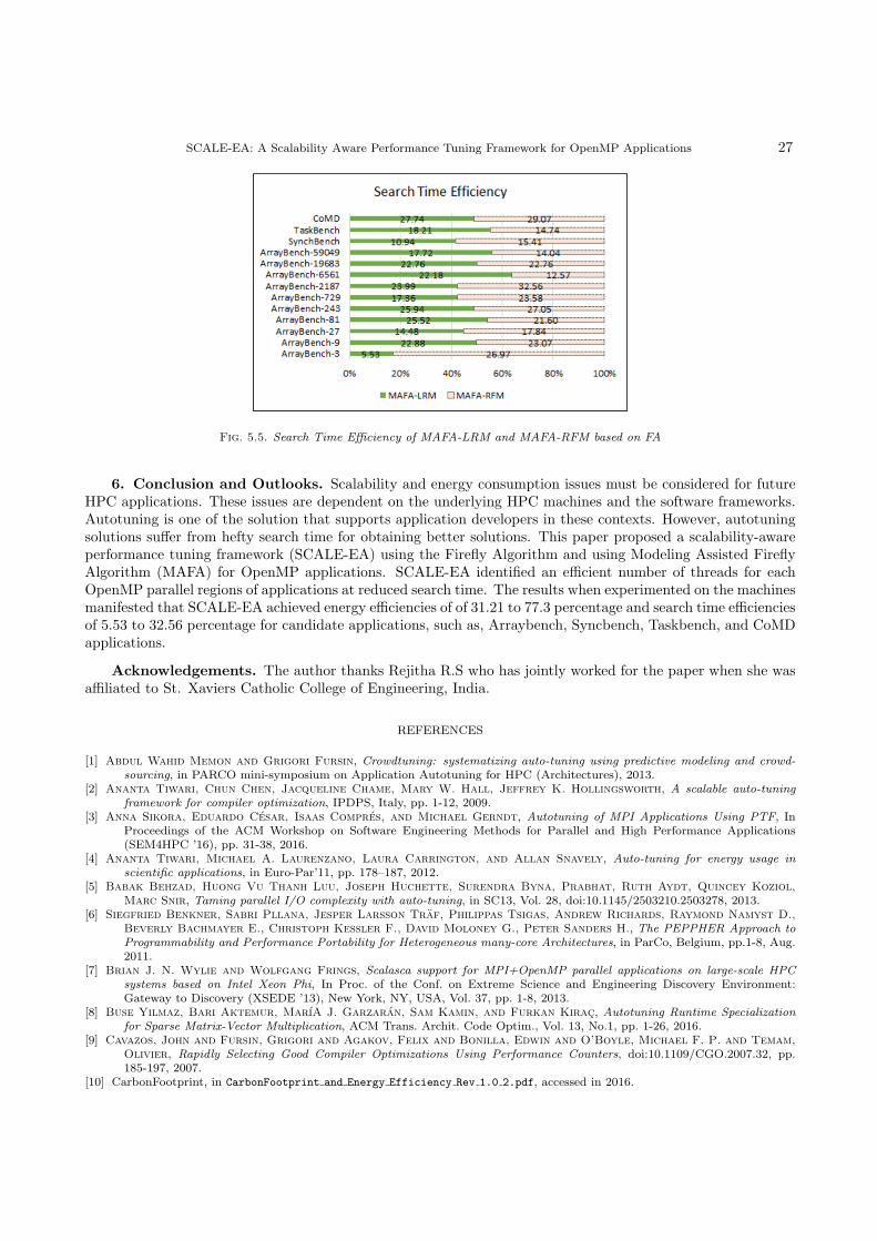
SCALE-EA: A Scalability Aware Performance Tuning Framework for OpenMP Applications 27
Fig. 5.5. Search Time Efficiency of MAFA-LRM and MAFA-RFM based on FA
6. Conclusion and Outlooks. Scalability and energy consumption issues must be considered for futureHPC applications. These issues are dependent on the underlying HPC machines and the software frameworks.Autotuning is one of the solution that supports application developers in these contexts. However, autotuningsolutions suffer from hefty search time for obtaining better solutions. This paper proposed a scalability-awareperformance tuning framework (SCALE-EA) using the Firefly Algorithm and using Modeling Assisted FireflyAlgorithm (MAFA) for OpenMP applications. SCALE-EA identified an efficient number of threads for eachOpenMP parallel regions of applications at reduced search time. The results when experimented on the machinesmanifested that SCALE-EA achieved energy efficiencies of of 31.21 to 77.3 percentage and search time efficienciesof 5.53 to 32.56 percentage for candidate applications, such as, Arraybench, Syncbench, Taskbench, and CoMDapplications.
Acknowledgements. The author thanks Rejitha R.S who has jointly worked for the paper when she wasaffiliated to St. Xaviers Catholic College of Engineering, India.
REFERENCES
[1] Abdul Wahid Memon and Grigori Fursin, Crowdtuning: systematizing auto-tuning using predictive modeling and crowd-sourcing, in PARCO mini-symposium on Application Autotuning for HPC (Architectures), 2013.
[2] Ananta Tiwari, Chun Chen, Jacqueline Chame, Mary W. Hall, Jeffrey K. Hollingsworth, A scalable auto-tuningframework for compiler optimization, IPDPS, Italy, pp. 1-12, 2009.
[3] Anna Sikora, Eduardo Cesar, Isaas Compres, and Michael Gerndt, Autotuning of MPI Applications Using PTF, InProceedings of the ACM Workshop on Software Engineering Methods for Parallel and High Performance Applications(SEM4HPC ’16), pp. 31-38, 2016.
[4] Ananta Tiwari, Michael A. Laurenzano, Laura Carrington, and Allan Snavely, Auto-tuning for energy usage inscientific applications, in Euro-Par’11, pp. 178–187, 2012.
[5] Babak Behzad, Huong Vu Thanh Luu, Joseph Huchette, Surendra Byna, Prabhat, Ruth Aydt, Quincey Koziol,
Marc Snir, Taming parallel I/O complexity with auto-tuning, in SC13, Vol. 28, doi:10.1145/2503210.2503278, 2013.[6] Siegfried Benkner, Sabri Pllana, Jesper Larsson Traf, Philippas Tsigas, Andrew Richards, Raymond Namyst D.,
Beverly Bachmayer E., Christoph Kessler F., David Moloney G., Peter Sanders H., The PEPPHER Approach toProgrammability and Performance Portability for Heterogeneous many-core Architectures, in ParCo, Belgium, pp.1-8, Aug.2011.
[7] Brian J. N. Wylie and Wolfgang Frings, Scalasca support for MPI+OpenMP parallel applications on large-scale HPCsystems based on Intel Xeon Phi, In Proc. of the Conf. on Extreme Science and Engineering Discovery Environment:Gateway to Discovery (XSEDE ’13), New York, NY, USA, Vol. 37, pp. 1-8, 2013.
[8] Buse Yilmaz, Bari Aktemur, MarıA J. Garzaran, Sam Kamin, and Furkan Kirac, Autotuning Runtime Specializationfor Sparse Matrix-Vector Multiplication, ACM Trans. Archit. Code Optim., Vol. 13, No.1, pp. 1-26, 2016.
[9] Cavazos, John and Fursin, Grigori and Agakov, Felix and Bonilla, Edwin and O’Boyle, Michael F. P. and Temam,
Olivier, Rapidly Selecting Good Compiler Optimizations Using Performance Counters, doi:10.1109/CGO.2007.32, pp.185-197, 2007.
[10] CarbonFootprint, in CarbonFootprint and Energy Efficiency Rev 1.0 2.pdf, accessed in 2016.

28 S. Benedict
[11] Cesar E., A. Moreno, J. Sorribes, E. Luque, Modeling Master/Worker applications for automatic performance tuning, inParallel Computing, Vol. 32, No. 78, pp. 568-589, 2006.
[12] Cheng Y., and Zeng Y., Automatic Energy Status Controlling with Dynamic Voltage Scaling in Power-Aware High Perfor-mance Computing Cluster, in proc. of 12th Int. Conf. on PDCAT, pp. 412 - 416, 2011.
[13] Cristina Silvano, Giovanni Agosta, Stefano Cherubin, Davide Gadioli, Gianluca Palermo, Andrea Bartolini, Luca
Benini, Jan Martinovic, Martin Palkovic, Katerina Slaninova, Joao Bispo, Joao M. P. Cardoso, Rui Abreu,
Pedro Pinto, Carlo Cavazzoni, Nico Sanna, Andrea R. Beccari, Radim Cmar, Erven Rohou, The ANTAREXapproach to autotuning and adaptivity for energy efficient HPC systems, in ACM International Conference on ComputingFrontiers, 2016.
[14] CoMD Application, from LLNL, USA, in http://www.exmatex.org/comd.html, accessed in Sep.2016.[15] Daniel A. Ellsworth, Allen D. Malony, Barry Rountree, Martin Schulz, POW: System-wide Dynamic Reallocation
of Limited Power in HPC, in Proc. of HPDC 2015, pp. 145-148, 2015.[16] Enes Bajrovic, Siegfried Benkner, Jir Dokulil, Martin Sandrieser, Autotuning of Pattern Runtimes for Accelerated
Parallel Systems, in Proc. of PARCO 2013, pp. 636-645, 2013.[17] EPCC OpenMP Benchmark suite, in https://www.epcc.ed.ac.uk/research/computing/performance-characterisation
-and-benchmarking/epcc-openmp-micro-benchmark-suite, accessed in Sep 2016.[18] Erika Abraham, Costas Bekas, Ivona Brandic, Samir Genaim, Einar Broch Johnsen, Ivan Kondov, Sabri Pllana,
and Achim Streit, Preparing HPC Applications for Exascale: Challenges and Recommendations, in ADPNA at NBiS, pp.1-6, 2015.
[19] Fister, I., Yang, X.S., Brest, J. and Fister Jr, I., Memetic self-adaptive firefly algorithm, in Swarm intelligence andbio-inspired computation: theory and applications, pp.73-102, 2013.
[20] Fister I., Yang X. S., Brest J., A comprehensive review of firefly algorithms, in Swarm and Evolutionary Computation,Vol. 13, pp. 34-46, 2013.
[21] Giorgio Luigi Valentini, Walter Lassonde, Samee Ullah Khan, Nasro Min-Allah, Sajjad A. Madani, Juan Li, Limin
Zhang, Lizhe Wang, Nasir Ghani, Joanna Kolodziej, Hongxiang Li, Albert Y. Zomaya, Cheng-Zhong Xu, Pavan
Balaji, Abhinav Vishnu, Fredric Pinel, Johnatan E. Pecero, Dzmitry Kliazovich, Pascal Bouvry, An overview ofenergy efficiency techniques in cluster computing systems, in Cluster Computing, Vol. No. 1, pp 315, 2013.
[22] Greg Faanes, Abdulla Bataineh, Duncan Roweth, Tom Court, Edwin Froese, Bob Alverson, Tim Johnson, Joe
Kopnick, Mike Higgins, and James Reinhard, Cray cascade: a scalable HPC system based on a Dragonfly network, InProceedings of the International Conference on High Performance Computing, Networking, Storage and Analysis (SC ’12),Los Alamitos, CA, USA, 9 pages, 2012.
[23] Guojing Cong, I-Hsin Chung, Hui-Fang Wen, David J. Klepacki, Hiroki Murata, Yasushi Negishi, Takao Moriyama:A Systematic Approach toward Automated Performance Analysis and Tuning, in IEEE Trans. Parallel Distrib. Syst., Vol.23, No. 3, pp. 426-435, 2012.
[24] Haihang You., Q. Liu, Z. Li, and S. Moore, The Design of an Auto-tuning I/O Framework on Cray XT5 System, in Proc.of Cray Users Group Conference (CUG’11) Alaska, May 2011.
[25] Jason Ansel, Shoaib Kamil, Kalyan Veeramachaneni, Jonathan Ragan-Kelley, Jeffrey Bosboom, Una-May
O’Reilly, and Saman Amarasinghe, OpenTuner: an extensible framework for program autotuning, In Proceedings ofthe 23rd international conference on Parallel architectures and compilation (PACT ’14), USA, pp. 303-316, 2014.
[26] Jee W. Choi, Amik Singh, and Richard W. Vuduc, Model-driven autotuning of sparse matrix-vector multiply on GPUs,In Proceedings of the 15th ACM SIGPLAN Symposium on Principles and Practice of Parallel Programming (PPoPP ’10),USA, pp. 115-126, 2010.
[27] Jordan, Herbert and Thoman, Peter and Durillo, Juan J. and Pellegrini, Simone and Gschwandtner, Philipp and
Fahringer, Thomas and Moritsch, Hans, A Multi-objective Auto-tuning Framework for Parallel Codes, Proc. of the Int.Conf. on HPC, Networking, Storage and Analysis, SC12, pp. 10:1-10:12, 2012.
[28] Knobloch M., Mohr B., and Minartz T., Determine energy-saving potential in wait-states of large-scale parallel programs,in Computer Sci. - Res. and Dev. pp. 1-9, 2011.
[29] Manish Parashar, Salim Hariri, Autonomic Computing: An Overview, in Unconventional Programming Paradigms, Vol.3566, LNCS, Springer, pp 257-269, 2005.
[30] Matthieu Doriera, Orcun Yildizc, Shadi Ibrahimc, Anne-Cecile Orgeried, Gabriel Antoniuc, On the energy footprintof I/O management in Exascale HPC systems, in FGCS, Vol. 62, pp. 17-28, 2016.
[31] Dark Silicon, in https://www.dagstuhl.de/en/program/calendar/semhp/?semnr=16052, 2016.[32] Pan Z. and Eigenmann R., Fast and effective orchestration of compiler optimizations for automatic performance tuning. In
Proc. of the Int. Symp. on Code Generation and Optimization, pages 319?332, 2006.[33] Prasanna Balaprakash, Stefan M. Wild, Boyanna Norris, SPAPT: Search Problems in Automatic Performance Tuning,
in Procedia Computer Science, Vol 9, pp. 1959 - 1968, 2012.[34] Robert Schone, Daniel Molka, and Michael Wern, Wake-up latencies for processor idle states on current x86 processors,
in Comput. Sci. Res. Dev. Vol. 30, pp. 219227, 2015.[35] Senthilnath J., Omkar S. N., Mani V., Clustering using firefly algorithm: performance study, in Swarm and Evolutionary
Computation, Vol. 1, No. 3, pp. 164-171, 2011.[36] Shajulin Benedict, Application of Energy Reduction Techniques using Niched Pareto GA of EnergyAnalzyer for HPC
Applications’, in 7th IEEE IC3 2014, http://dx.doi.org/10.1109/IC3.2014.6897234, 2014.[37] Shajulin Benedict, Threshold Acceptance Algorithm based Energy Tuning of Scientific Applications using EnergyAnalyzer,
ISEC2014, ACM publishers, 2014.[38] Shajulin Benedict, Rejitha R.S., Phillip G., Radu Prodan, Thomas Fahringer, Energy Prediction of OpenMP Ap-

SCALE-EA: A Scalability Aware Performance Tuning Framework for OpenMP Applications 29
plications using Random Forest Modeling Approach, in iWAPT2015 @ IPDPS 2015 DOI 10.1109/IPDPSW.2015.12, pp.1251-1260, 2015.
[39] Sukhyun Song and Jeffrey K. Hollingsworth, Computationcommunication overlap and parameter auto-tuning for scalableparallel 3-D FFT, in Journal of Computational Science, Vol. 14, pp. 3850, 2016.
[40] Weifeng Liu, Michael Gerndt, Bin Gong, Model-based MPI-IO tuning with Periscope tuning framework, Concurrency andComp.: Prac. and Exp., Vol. 28, No.1, pp: 3-20, 2016.
[41] Xin-She Yang, Firefly algorithm, stochastic test functions and design optimisation, in Int. Journal of Bioinspired Computa-tion, Vol. 2, No. 2, pp. 78-84, 2010.
[42] Yury Oleynik, Michael Gerndt, Joseph Schuchart, Per Gunnar Kjeldsberg, and Wolfgang E. Nagel, Run-TimeExploitation of Application Dynamism for Energy-Efficient Exascale Computing (READEX), CSE 2015, pp:347-350, 2015.
Edited by: Dana PetcuReceived: Oct 17, 2017Accepted: Dec 23, 2017


Scalable Computing: Practice and Experience
Volume 19, Number 1, pp. 31–38. http://www.scpe.org
DOI 10.12694/scpe.v19i1.1391ISSN 1895-1767c⃝ 2018 SCPE
GPU-BASED ACCELERATION OF METHODS BASED ON CLOCK MATCHING METRIC
FOR LARGE SCALE 3D SHAPE RETRIEVAL
MOHAMMED BENJELLOUN∗, EL WARDANI DADI†, AND EL MOSTAFA DAOUDI ‡
Abstract. In this paper, we exploit the potential of the GPU in order to accelerate the process of 3D shape retrieval in largedatabases. Indeed, the massive parallelism of the GPU offers a huge performance in much high-performance computing (HPC)applications. Our solution consists to accelerate the shape matching process of methods that use a specific similarity metric calledClock Matching (CM). This CM measure is used by view-based methods as an efficient solution to compare two 3D models evenif they are not presented in same pose and orientation by taking into account all possible poses in the matching phase. However,the increase in the number of comparisons has a strong influence on the execution time. Our challenge is to exploit the maximumbenefit of GPU computing resource by considering the difficulty of implementing the CM metric on GPU. Indeed, the descriptorof a given 3D object is organized using a specific data structure (hash table), where only the information whose values are notequal to zero appears in the feature vector, which makes the parallelization on GPU to be not trivial. Experiment results show areasonable benefit from the GPU approach.
Key words: GPU, 3D Shape retrieval, Clock Matching, CM-BOF, CM-VGG, 3D object.
AMS subject classifications. 68W10, 68P05
1. Introduction. Thanks to the current digitizing and modeling technologies, the number of accessibleand available 3D models on the web is increasing, which yielded large databases of 3D models. This has ledto the development of 3D shape retrieval systems [1, 7, 6, 9, 10, 12, 14, 15, 16] that, given a query object,retrieve similar 3D models. These systems work into two essentials phases which are shape indexing and shapematching. The first one consists to compute the descriptor of a given 3D object while the second one, consiststo compare the query object with the 3D models in the database. For most of 3D shape retrieval method, thek objects similar to the query are returned until the shape matching is done with the whole 3D objects in thedatabase. When the dataset size gets very large, the shape matching process becomes very challenging. Thechallenges come especially from the augmentation of computational time.
In order to accelerate the retrieval process, various content-based retrieval methods and approaches havebeen proposed in the literature [1, 2, 3, 4, 8, 14, 16]. Including sequential solutions [1, 4] and those based onhigh-performance computing, like multi-core [3]and GPU[2, 8], ... Despite the high-efficiency of HPC solutions,the problem is that there are a few works in the literature that implement the 3D shape retrieval under GPUenvironment, most of them are partial since they only concern the shape indexing phase [8].
To accelerate the shape matching phase we have already proposed a GPU-based implementation [2], of agiven 3D shape retrieval method called BF-SIFT [11]. The solution proposed in [2] is general and it can beapplied to several methods based on the same similarity metric which is KLD (Kullback-Leibler divergence),such as Euclidean distance.
In this paper, we propose a GPU-based implementation of a specific similarity metric called Clock Matching(CM). This similarity measure is used by two view-based methods which are CM-BOF proposed by [10], andCM-VGG presented in [14]. The only difference between the two methods is in the way they do shape indexing,the first one uses Bag-Of-Feature [5, 10, 11] while the second one uses the deep learning approach [14]. TheCM metric is the common point between them, its basic idea is to compare two 3D objects even if they arepresented in different poses and directions by doing a set of comparison according to 24 different poses still existfor a normalized model. This technique permits to overcome the problem of the alignment and the reflexion.However, the increase in the number of comparisons is a very critical point with a strong influence on theexecution time.
∗Department of Computer Science, Faculty of Engineering University of Mons, BELGIUM. ([email protected]).
†National School of Applied Sciences, LaRi Laboratory, University of Mohammed First, MOROCCO.([email protected]). Ques-tions, comments, or corrections to this document may be directed to that email address.
‡Faculty of Sciences, LaRi Laboratory, University of Mohammed First, MOROCCO.([email protected]).
31

32 M. Benjelloun, E. W. Dadi, E. M. Daoudi
Fig. 1.1. An example of the used two types of data,(a) Indexed structure,(b) Specific structure
Our challenge is to adapt the CM metric to be performed on GPU. Indeed, the difficulty of this implemen-tation is that the feature vector of a given 3D object is organized using a specific data structure cf. Figure 1.1.b,which makes the parallelization GPU to be not trivial. Note that as our contribution concerns not only theCM approach but it resolves the problem of how performing a metric between specific data-structure as a hashtable on the GPU.
The rest of the paper is organized as follows. Sect. 2 is devoted to the related works. In Sect. 3 we give abrief description of the Clock matching technique. Our proposed implementation is presented in Sect. 4. Sect. 5is devoted to the experimental results. We conclude the paper in Sect. 6.
2. Related works. 3D shape content-based retrieval in large datasets is an active research topic relatedto different fields such as computer vision and pattern recognition,... Indeed, large databases of multimediadata have become available on the web. However, when the dataset size gets very large, the retrieving processbecomes very challenging. The challenges come from storage, computation speed, and features representation.Various methods and techniques have been proposed in the literature to accelerate the process of retrieving[1, 2, 3, 4, 8, 14, 16]. The different solutions proposed can be classified into two categories:
• Solutions based on sequential approaches: as an example of these solutions, our proposed work [4],the idea is, for a classified database, we represent each class by a representative in order to orient theprocess of matching only in the classes of which its representative is the most similar to query. In otherwork [1], we have proposed an approach that can reduce the number of comparisons of the query in thedatabase.
• Solutions based on high-performance computing(HPC), for multi-core architecture, the idea presentedin [3] is to compare the query object simultaneously with P objects, where P is the number of processors.For GPU solutions, Wu [8] have proposed an implementation of SIFT algorithm, this solution is partialbecause it concerns only a step of shape indexing process and not the shape matching process. Toour knowledge, the only work that dealt with the shape matching process on GPU is [2], in which wehave proposed a GPU-based implementation of an existing method called BF-SIFT [11]. This solutionis general it can be applied to different well-known dissimilarity measurements such as Euclidean L2,Minkowski.
3. Description of the Clock Matching metric. The Clock matching is a specific similarity metricemployed for the first time by the CM-BOF [10] method to compare descriptors of two 3D objects. Recently,it’s used in SHREC’17 Track by the CM-VGG method [14]. The CM-BOF and CM-VGG are both view-basedmethods and the only difference between them is in the way that’s used to characterize the shape of a given 3Dobject. The first one uses the Bag-Of-Features approach [5, 10, 11] while the second one uses the deep learningapproach [14].
To characterize a given 3D object, these view-based methods capture a set of 2D view around its 3D shapeusing a virtual camera. Each 2D view is described as a feature vector of one dimension. Fortunately, for thetwo case, in CM-BOF and in CM-VGG, the feature vector produced is a very sparsely populated histogram,
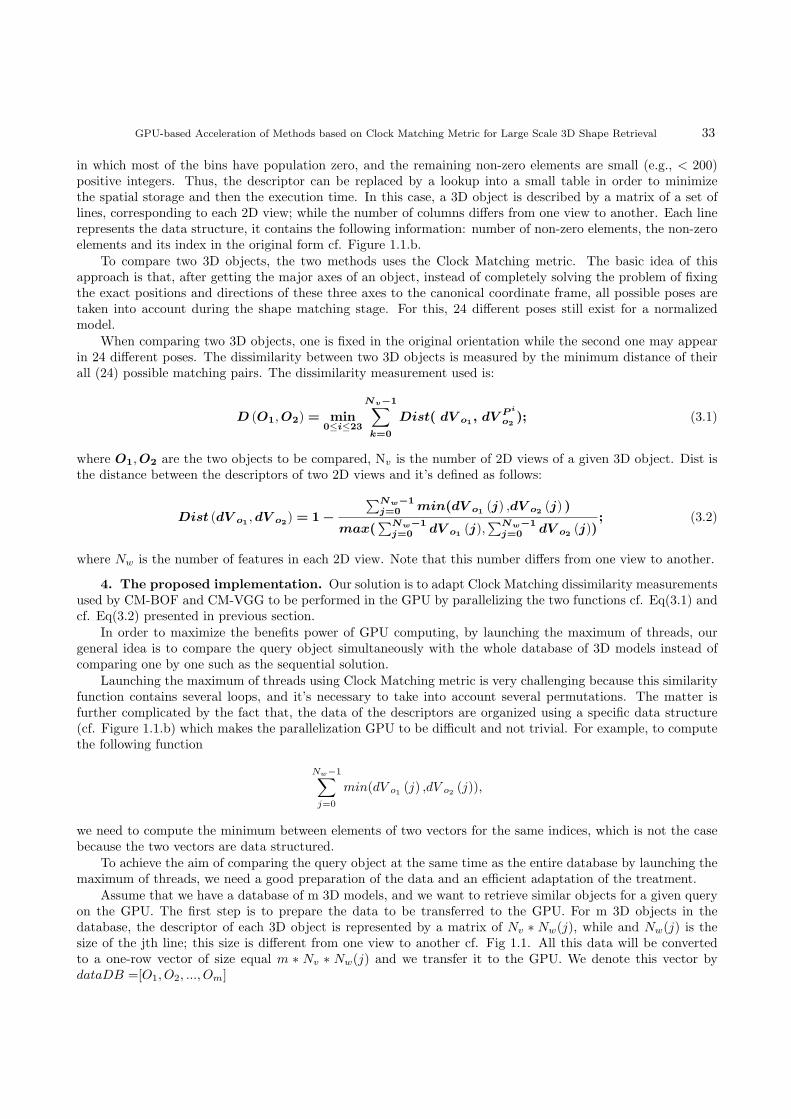
GPU-based Acceleration of Methods based on Clock Matching Metric for Large Scale 3D Shape Retrieval 33
in which most of the bins have population zero, and the remaining non-zero elements are small (e.g., < 200)positive integers. Thus, the descriptor can be replaced by a lookup into a small table in order to minimizethe spatial storage and then the execution time. In this case, a 3D object is described by a matrix of a set oflines, corresponding to each 2D view; while the number of columns differs from one view to another. Each linerepresents the data structure, it contains the following information: number of non-zero elements, the non-zeroelements and its index in the original form cf. Figure 1.1.b.
To compare two 3D objects, the two methods uses the Clock Matching metric. The basic idea of thisapproach is that, after getting the major axes of an object, instead of completely solving the problem of fixingthe exact positions and directions of these three axes to the canonical coordinate frame, all possible poses aretaken into account during the shape matching stage. For this, 24 different poses still exist for a normalizedmodel.
When comparing two 3D objects, one is fixed in the original orientation while the second one may appearin 24 different poses. The dissimilarity between two 3D objects is measured by the minimum distance of theirall (24) possible matching pairs. The dissimilarity measurement used is:
D (O1,O2) = min0≤i≤23
Nv−1∑
k=0
Dist( dV o1, dV P i
o2); (3.1)
where O1,O2 are the two objects to be compared, Nv is the number of 2D views of a given 3D object. Dist isthe distance between the descriptors of two 2D views and it’s defined as follows:
Dist (dV o1,dV o2
) = 1−
∑Nw−1
j=0min(dV o1
(j) ,dV o2(j) )
max(∑Nw−1
j=0dV o1
(j),∑Nw−1
j=0dV o2
(j)); (3.2)
where Nw is the number of features in each 2D view. Note that this number differs from one view to another.
4. The proposed implementation. Our solution is to adapt Clock Matching dissimilarity measurementsused by CM-BOF and CM-VGG to be performed in the GPU by parallelizing the two functions cf. Eq(3.1) andcf. Eq(3.2) presented in previous section.
In order to maximize the benefits power of GPU computing, by launching the maximum of threads, ourgeneral idea is to compare the query object simultaneously with the whole database of 3D models instead ofcomparing one by one such as the sequential solution.
Launching the maximum of threads using Clock Matching metric is very challenging because this similarityfunction contains several loops, and it’s necessary to take into account several permutations. The matter isfurther complicated by the fact that, the data of the descriptors are organized using a specific data structure(cf. Figure 1.1.b) which makes the parallelization GPU to be difficult and not trivial. For example, to computethe following function
Nw−1∑
j=0
min(dV o1 (j) ,dV o2 (j)),
we need to compute the minimum between elements of two vectors for the same indices, which is not the casebecause the two vectors are data structured.
To achieve the aim of comparing the query object at the same time as the entire database by launching themaximum of threads, we need a good preparation of the data and an efficient adaptation of the treatment.
Assume that we have a database of m 3D models, and we want to retrieve similar objects for a given queryon the GPU. The first step is to prepare the data to be transferred to the GPU. For m 3D objects in thedatabase, the descriptor of each 3D object is represented by a matrix of Nv ∗ Nw(j), while and Nw(j) is thesize of the jth line; this size is different from one view to another cf. Fig 1.1. All this data will be convertedto a one-row vector of size equal m ∗ Nv ∗ Nw(j) and we transfer it to the GPU. We denote this vector bydataDB =[O1, O2, ..., Om]

34 M. Benjelloun, E. W. Dadi, E. M. Daoudi
Regrouping all the data of m 3D objects as one vector will raise the problem of how to determinate thesize of each jth line corresponding to each 2D view. To overcome this problem, our idea is to keep the data ofthe query object in the original form without structuring it. In this case, the query object is represented by amatrix of size Nw ∗Nv while Nw is the size of the descriptor of each 2D view. Since the indexing process of theobject query is performed online, our solution that consists of keeping the initial form permits to reduce theexecution time allowed to the structuring process.
So, after transferring the dataDB to GPU, we transfer the data of query object as one vector of Nw ∗Nv
which we denote dataQuery.
To perform the shape matching on the GPU, by taking into account the exploiting of the maximum ofGPU computing power, our solution consists to separate the treatment of the two functions cf. Eq(3.1) and cf.Eq(3.2) as follows:
• Step 1: we calculate the function∑Nw−1
j=0min(dV o1 (j) ,dV o2 (j))
• Step 2: we calculate the function max(∑Nw−1
j=0dV o1 (j),
∑Nw−1
j=0dV o2 (j))
• Step 3: we calculate the distance: Dist (dV o1 , dV o2)• Step 4: we calculate the distance: D (O1, O2)• Step 5: we sort the obtained distance D.
Several kernels are used to calculate the different functions on GPU such as:
1. Kernel 1 is used to compute the minimum between pair of elements of two vectors2. Kernel 2 is used to compute the maximum between pair of elements of two vectors3. Kernel 3 is used to compute the sum of elements of a given vector.4. Kernel 4 is used to compute the division between pair of elements of two vectors
Each step of the five steps has its special adaptation on GPU. To clarify this, we will explain step by step.
4.1. Step 1. For the first step which is∑Nw−1
j=0min(dV o1 (j) ,dV o2 (j)), we use two kernels (kernel 1 and
kernel 2). The first one is to compute the minimum function and the second one to calculate the summation ofresults obtained by the first kernel.
4.1.1. The minimum function. Instead of computing the minimum between two descriptors one byone and sequentially, our solution is to compute this minimum function simultaneously and in the same timebetween query and all objects in the database. Our idea is to launch a m*Nv*Nw(j)*24 threads on GPU eachone will execute following instruction:
if(dataQuery[]<dataDB[])Result[]=dataQuery[ ]
elseResult[]=dataDB[]
The problem with launching these numbers of threads simultaneously is how to control access index tovector elements because the size of each row in the database is different from one line to another cf. Figure 1.1.For example, assume we have launched 18 threads to compute the minimum between the two vectors presentedin cf. Figure 1.1, for the first four threads there is no problem, each one will execute its instruction as follows:
Thread 1 Thread 2dataQuery[0]<dataDB[0]) dataQuery[1]<dataDB[1]
Thread 3 Thread 4dataQuery[2]<dataDB[2]) dataQuery[3]<dataDB[3]
The problem start with the second line of the matrix, it consists of determining the index that permits theaccess to the second line of query matrix. To overcome this problem our solution is to generate two vectors :
• The first one is to control the acces to information in dataDB, its size is equal to the size of the databasedata (m ∗ Nv ∗ Nw(j) ); we call it TableSize. Note that as this operation is performed offline. Thisvector is generated as follows:
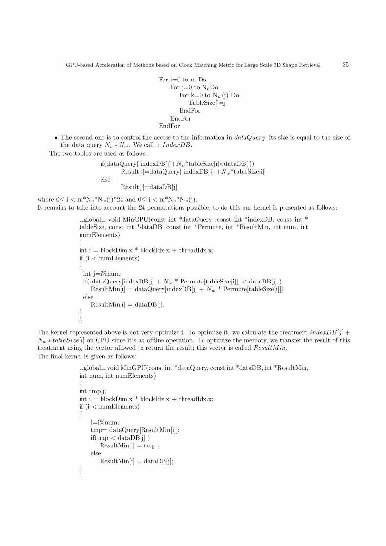
GPU-based Acceleration of Methods based on Clock Matching Metric for Large Scale 3D Shape Retrieval 35
For i=0 to m DoFor j=0 to NvDo
For k=0 to Nw(j) DoTableSize[]=j
EndForEndFor
EndFor
• The second one is to control the access to the information in dataQuery, its size is equal to the size ofthe data query Nv ∗Nw. We call it IndexDB.
The two tables are used as follows :
if(dataQuery[ indexDB[j]+Nw*tableSize[i]<dataDB[j])Result[j]=dataQuery[ indexDB[j] +Nw*tableSize[i]]
elseResult[j]=dataDB[j]
where 0≤ i < m*Nv*Nw(j)*24 and 0≤ j < m*Nv*Nw(j).
It remains to take into account the 24 permutations possible, to do this our kernel is presented as follows:
global void MinGPU(const int *dataQuery ,const int *indexDB, const int *tableSize, const int *dataDB, const int *Permute, int *ResultMin, int num, intnumElements){int i = blockDim.x * blockIdx.x + threadIdx.x;if (i < numElements){int j=i%num;if( dataQuery[indexDB[j] + Nw * Permute[tableSize[i]]] < dataDB[j] )
ResultMin[i] = dataQuery[indexDB[j] + Nw * Permute[tableSize[i]]];else
ResultMin[i] = dataDB[j];}}
The kernel represented above is not very optimized. To optimize it, we calculate the treatment indexDB[j] +Nw ∗ tableSize[i] on CPU since it’s an offline operation. To optimize the memory, we transfer the result of thistreatment using the vector allowed to return the result; this vector is called ResultMin.
The final kernel is given as follows:
global void MinGPU(const int *dataQuery, const int *dataDB, int *ResultMin,int num, int numElements){int tmp,j;int i = blockDim.x * blockIdx.x + threadIdx.x;if (i < numElements){
j=i%num;tmp= dataQuery[ResultMin[i]];if(tmp < dataDB[j] )
ResultMin[i] = tmp ;else
ResultMin[i] = dataDB[j];}}
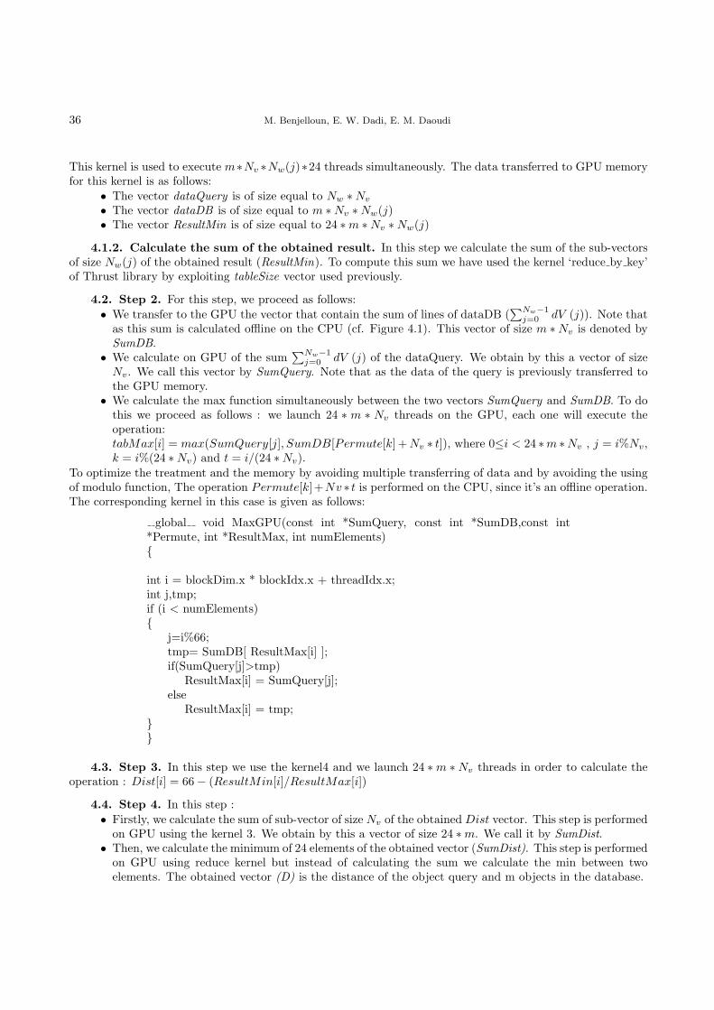
36 M. Benjelloun, E. W. Dadi, E. M. Daoudi
This kernel is used to execute m∗Nv ∗Nw(j)∗24 threads simultaneously. The data transferred to GPU memoryfor this kernel is as follows:
• The vector dataQuery is of size equal to Nw ∗Nv
• The vector dataDB is of size equal to m ∗Nv ∗Nw(j)• The vector ResultMin is of size equal to 24 ∗m ∗Nv ∗Nw(j)
4.1.2. Calculate the sum of the obtained result. In this step we calculate the sum of the sub-vectorsof size Nw(j) of the obtained result (ResultMin). To compute this sum we have used the kernel ‘reduce by key’of Thrust library by exploiting tableSize vector used previously.
4.2. Step 2. For this step, we proceed as follows:
• We transfer to the GPU the vector that contain the sum of lines of dataDB (∑Nw−1
j=0dV (j)). Note that
as this sum is calculated offline on the CPU (cf. Figure 4.1). This vector of size m ∗Nv is denoted bySumDB.
• We calculate on GPU of the sum∑Nw−1
j=0dV (j) of the dataQuery. We obtain by this a vector of size
Nv. We call this vector by SumQuery. Note that as the data of the query is previously transferred tothe GPU memory.
• We calculate the max function simultaneously between the two vectors SumQuery and SumDB. To dothis we proceed as follows : we launch 24 ∗ m ∗ Nv threads on the GPU, each one will execute theoperation:tabMax[i] = max(SumQuery[j], SumDB[Permute[k] +Nv ∗ t]), where 0≤i < 24 ∗m ∗Nv , j = i%Nv,k = i%(24 ∗Nv) and t = i/(24 ∗Nv).
To optimize the treatment and the memory by avoiding multiple transferring of data and by avoiding the usingof modulo function, The operation Permute[k]+Nv ∗ t is performed on the CPU, since it’s an offline operation.The corresponding kernel in this case is given as follows:
global void MaxGPU(const int *SumQuery, const int *SumDB,const int*Permute, int *ResultMax, int numElements){
int i = blockDim.x * blockIdx.x + threadIdx.x;int j,tmp;if (i < numElements){
j=i%66;tmp= SumDB[ ResultMax[i] ];if(SumQuery[j]>tmp)
ResultMax[i] = SumQuery[j];else
ResultMax[i] = tmp;}}
4.3. Step 3. In this step we use the kernel4 and we launch 24 ∗m ∗Nv threads in order to calculate theoperation : Dist[i] = 66− (ResultMin[i]/ResultMax[i])
4.4. Step 4. In this step :
• Firstly, we calculate the sum of sub-vector of size Nv of the obtained Dist vector. This step is performedon GPU using the kernel 3. We obtain by this a vector of size 24 ∗m. We call it by SumDist.
• Then, we calculate the minimum of 24 elements of the obtained vector (SumDist). This step is performedon GPU using reduce kernel but instead of calculating the sum we calculate the min between twoelements. The obtained vector (D) is the distance of the object query and m objects in the database.
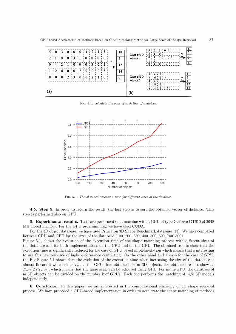
GPU-based Acceleration of Methods based on Clock Matching Metric for Large Scale 3D Shape Retrieval 37
Fig. 4.1. calculate the sum of each line of matrices.
100 200 300 400 500 600 700 800Number of objects
0.0
0.5
1.0
1.5
2.0
2.5
Exec
ution tim
e
GPUCPU
Fig. 5.1. The obtained execution time for different sizes of the database.
4.5. Step 5. In order to return the result, the last step is to sort the obtained vector of distance. Thisstep is performed also on GPU.
5. Experimental results. Tests are performed on a machine with a GPU of type GeForce GT610 of 2048MB global memory. For the GPU programming, we have used CUDA.
For the 3D object database, we have used Princeton 3D Shape Benchmark database [13]. We have comparedbetween CPU and GPU for the sizes of the database (100, 200, 300, 400, 500, 600, 700, 800).Figure 5.1, shows the evolution of the execution time of the shape matching process with different sizes ofthe database and for both implementations on the CPU and on the GPU. The obtained results show that theexecution time is significantly reduced for the case of GPU based implementation which means that’s interestingto use this new resource of high-performance computing. On the other hand and always for the case of GPU,the Fig Figure 5.1 shows that the evolution of the execution time when increasing the size of the database isalmost linear; if we consider Tm as the GPU time obtained for m 3D objects, the obtained results show asTm≈(2 ∗ Tm/2), which means that the large scale can be achieved using GPU. For multi-GPU, the database ofm 3D objects can be divided on the number k of GPUs. Each one performs the matching of m/k 3D modelsindependently.
6. Conclusion. In this paper, we are interested in the computational efficiency of 3D shape retrievalprocess. We have proposed a GPU-based implementation in order to accelerate the shape matching of methods

38 M. Benjelloun, E. W. Dadi, E. M. Daoudi
that use Clock Matching metric. This implementation exploits the maximum of the potential of the GPUand it permits to compare simultaneously, the query object with a large number of 3D models. This hasthe advantages of obtaining the retrieval results in a very short time, the thing that was well justified by theexperimental results. Experimental results show that the execution time is significantly reduced compared tothe execution on the CPU. Our proposed solution shows that the large-scale retrieval can be achieved usingGPU.
REFERENCES
[1] M. Benjelloun, E. W. Dadi, and E. M. Daoudi, New approach for efficiently retrieving similar 3D models based on reducingthe research space. International Journal of Imaging 01/2014; 13(2), pages 104-111.
[2] E. W. Dadi and E. M. Daoudi, GPU-Based for accelerating the BF-SIFT method for large-scale 3D shape retrieval, MultimediaComputing, and Systems (ICMCS), 2014 International Conference on, Marrakech, 2014, pages 38-41.
[3] E. W. Dadi, and E. M. Daoudi. Large Scale 3D Shape Retrieval Based on Multi-core Architectures, Lecture Notes in ComputerScience 7853, 2013, pages 295-299.
[4] E. W. Dadi, E. M. Daoudi, and C. Tadonki. Fast 3D shape retrieval method for classified databases, IEEE InternationalConference on Complex Systems (ICCS) 2012.
[5] J. Fehr, A. Streicher and H. Burkhardt, A Bag of Features Approach for 3D Shape Retrieval, Advances in Visual Com-puting, Lecture Notes in Computer Science, 2009, pages 34-43.
[6] T. A. Funkhouser, M. Kazhdan, P. Min, P. Shilane, Shape-based retrieval and analysis of 3D models, Communications ofthe ACM - 3d hard copy, Volume 48 Issue 6, June 2005, pages 58-64.
[7] Y. Gao, Q. Dai, M. Wang, N. Zhang, 3D model retrieval using weighted bipartite graph matching, Signal Processing: ImageCommunication Journal Volume 26 Issue 1, January, 2011, pages 39-47.
[8] C. Wu, A GPU Implementation of Scale Invariant Feature Transform (SIFT), http://cs.unc.edu/˜ccwu/siftgpu[9] A. Koutsoudis, C. Chamzas, 3D pottery shape matching using depth map images, Journal of Cultural Heritage, Journal of
Cultural Heritage, Volume 12, Issue 2, AprilJune 2011, pages 128-133.[10] Z. Lian, A. Godil, X. Sun and J. Xiao, CM-BOF: visual similarity-based 3D shape retrieval using Clock Matching and
Bag-of-Features, Journal of Machine Vision and Applications; Vol. 24 Issue 8, Nov 2013, p1685 ISBN 0932-8092.[11] R. Ohbuchi, K. Osada, T. Furuya, T. Banno, Salient Local Visual Features for Shape-Based 3D Model Retrieval, IEEE
International Conference on Shape Modeling and Applications (SMI08), Stony Brook University, June 4-6, 2008.[12] L. Pengjie, H. Ma, and A. Ming, Nonrigid 3D model retrieval using multi-scale local features, Proceedings of the 19th ACM
international conference on Multimedia - MM 11, 2011.[13] P. Shilane, P. Min, M. Kazhdan, and T. A. Funkhouser, The Princeton shape benchmark, in Shape Modeling and
Applications Conference, SMI2004, Genova, Italy, June 2004, IEEE, pp. 167178.[14] M. Savva, F. Yu, H. Su, A.Kanezaki, T. Furuya, R. Ohbuchi, Z. Zhou, R. Yu, S. Bai, X. Bai5, M. Aono, A. Tatsuma,
S. Thermos, A. Axenopoulos, G. Th. Papadopoulos, P. Daras, X. Deng, Z. Lian, B. Li, H. Johan, and Y. Lu,
S. Mk, SHREC17 Track Large-Scale 3D Shape Retrieval from ShapeNet Core55, Eurographics Workshop on 3D ObjectRetrieval 2017.
[15] J.W.H. Tangelder and R.C. Veltkamp, A survey of content based 3D shape retrieval methods, Multimedia Tools andApplications, vol. 39, no. 3, pp. 441471, Sept. 2008.
[16] R. C. Veltkamp, G. J. Giezeman, H. Bast, T. Baumbach, T. Furuya, J. Giesen, A. Godil, Z. Lian, R. Ohbuchi, W.
Saleem, SHREC10 Track: Large Scale Retrieval, Eurographics Workshop on 3D Object Retrieval 2010.
Edited by: Dana PetcuReceived: Oct 10, 2017Accepted: Feb 16, 2018
Scalable Computing: Practice and Experience
Volume 19, Number 1, pp. 39–51. http://www.scpe.org
DOI 10.12694/scpe.v19i1.1392ISSN 1895-1767c⃝ 2018 SCPE
ROUND ROBIN WITH LOAD DEGREE: AN ALGORITHM FOR OPTIMAL
CLOUDLET DISCOVERY IN MOBILE CLOUD COMPUTING
RAMASUBBAREDDY SOMULA∗AND SASIKALA R†
Abstract. Mobile devices have become essential in our daily lives but it has limited resources such as battery life, storage, andprocessing capacity. Offloading resource intensive task into the cloud is an efficient approach to improve battery utilization, storagecapacity and processing capabilities. Efficiently computing using cloud resources to process offloaded task in order to improveresponse time and reduce both tasks’ waiting time and latency problems is one of the main goals in mobile cloud computing(MCC). In order to improve user satisfaction and performance of the mobile application, a cloudlet framework concept has beendeveloped to reduce latency problems which improve response time. The cloudlet brings the cloud closer to the user to perform acomputational task. This article proposes a new balancing model among cloudlets in mobile cloud computing environment to findthe required resources and create an impact on performance. The efficient load balancing model makes mobile cloud computing moreattractive and improves user satisfaction. This paper introduces a Round Robin with Load degree algorithm for public cloudletsin mobile cloud computing using a switch mechanism to choose different approaches for different situations. This algorithm usesgame theory based load balancing approach to improve application response time in public mobile cloud environments.
Key words: public cloud; cloudlet, offloading, mobile cloud computing, load balancing model, game theory
AMS subject classifications. 68M14, 91A80
1. Introduction. Mobile cloud computing (MCC) can be viewed as a resource to fill the gap betweenlimited resources of mobile devices (MD) and computation requirement of MD. According to the definitionprovided by [9], mobile cloud computing is a task in which both computation and storage will happen outsideof smart device. The mobile cloud computing has attracted the attention of industries do to its benefits. Itreduces the efforts in developing application and also allows users to use the latest technology on demand basis(or) pay per use model. The MCC has three main components: mobile device, wireless connection, cloudinfrastructure where both data storage and processing power will be available. Computation offloading meansthat a computation part of mobile application is offloaded into remote cloud for execution in order to extendmobile device capabilities. Computation offloading can be sufficient when network connection is good and cloudprovides enough resources [31]. The cloud provides resource to MD with the help of network communication inheterogeneous environment [22].
The cloudlet is an emerging technology in mobile cloud computing that brings cloud near to mobile user(being like a data center in the box). The cloudlet is based on a cluster of physical machines which allowsnearby mobile users to use available resources [24]. It can be available around mobile users. Figure 1.1 depictsthe cloudlet architecture: a cloudlet is a kind of small scale server, associated with specific resources. This canbe accessed by mobile devices within specific range. The cloudlet provides cloud resources to users in a shorttime and with a certain level of throughputs [15].
The cloudlet can be composed of three layers: component layer, node layer and cloudlet layer. The compo-nent layer provides resources to higher layer through interface overlooked by execution environment. The nodecan be formed by running a node agent on one or more execution environments on the top of OS. Multiplenodes can be formed as cloudlet by a cloudlet agent [27].
The cloudlet can be efficient and scalable, but maintaining and processing a large number of incoming jobsconsistently is very difficult. Therefore, the researchers are paying attention to the load balancing problem.The behavior of the incoming jobs from mobile users is unpredictable and each cloudlet capabilities cannot beconstant (number of physical systems can always be changed). In order to improve the system performance andmaintain stability, controlling the workload distributed among cloudlets is very important.
Load balancing mechanisms can be classified into two types: static and dynamic [25]. In case of static,the mechanism is simple and does not consider nodes performance before distributing load into heterogeneousenvironment and handles nodes showing low load variation while dynamic mechanism uses nodes performance
∗School of Computer Science and Engineering (SCOPE), VIT University, Vellore, India ([email protected]).†School of Computer Science and Engineering (SCOPE), VIT University, Vellore, India.([email protected])
39

40 R. Somula, Sasikala R
Fig. 1.1. Cloudlet Architecture
while distributing work load. Dynamic nature algorithms are more complex than static nature algorithms. Thebehavior of dynamic scheme is changing according to node status or performance and brings additional cost.
In our model, the proposed method also follows dynamic load balancing as the load is distributed withprogression of time. The proposed model contains a cloudlet manager cloudlet agents. The cloudlet managerdirects the jobs from users to cloudlet. The cloudlet agent collects the information of cloudlet and updates thestatus in cloudlet manager. The dynamic model is using system status and decides the best balancing strategy.This process will influence other working nodes in cloudlet. The Load balancing model is mainly based on publiccloud environment. The cloudlets are distributed in geographical locations. The Cloudlet manager maintainsdistributed cloudlets and each cloudlet is assigned to one agent. The Cloudlet manager will select a cloudlet forincoming jobs and agent decides load balancing strategy. The existing algorithms allocate arriving jobs frommobile users to available cloudlets without knowing the status of the cloudlet. These makes jobs to wait forlong time in queue until other jobs get finished. To address this problem a new balancing algorithm is proposedin this paper. The proposed algorithm computes Load degree of each node in cloudlet to drive the incomingjobs to a particular cloudlet in geographical area.
2. Background. Ofloading mobile application into remote cloud to avoid limitation of mobile devices andincreases the performance of application was studied in [4, 23, 20, 19]. There are many mechanisms introducedto find when the task should offload on cloudlet [5, 8, 11, 26]. Usually, the model for offloading mobileapplication into remote cloud consists of components for both client and server. The client components work onmobile devices at client side whereas server components at remote cloud. The client side components monitornetwork performance, predicts the computational resources of mobile application and estimating time for localas well as remote execution times. By using this information the client components make decisions on how muchportion of the application to offload [7, 8]. The task offloading can be done by migrating VM from one cloudletto another cloudlet [13]. The recent works ThinkAir [17], cloudclone [7], proposed the concept of offloadingmobile application from single-machine execution into distributed execution environment automatically. Thestudy of the efficient model for offloading task solution to improve QoS of user application is done in [14]. Theusers are able to offload tasks into a cloudlet by selection, in the papers [28, 29], [6]. There are studies which aremainly focused to minimize revenue of service providers in cloud using linear programming model for offloading.
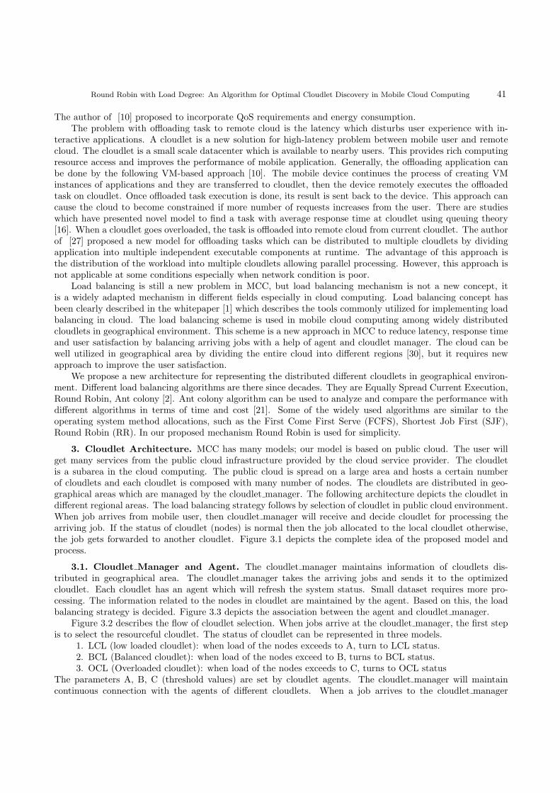
Round Robin with Load Degree: An Algorithm for Optimal Cloudlet Discovery in Mobile Cloud Computing 41
The author of [10] proposed to incorporate QoS requirements and energy consumption.The problem with offloading task to remote cloud is the latency which disturbs user experience with in-
teractive applications. A cloudlet is a new solution for high-latency problem between mobile user and remotecloud. The cloudlet is a small scale datacenter which is available to nearby users. This provides rich computingresource access and improves the performance of mobile application. Generally, the offloading application canbe done by the following VM-based approach [10]. The mobile device continues the process of creating VMinstances of applications and they are transferred to cloudlet, then the device remotely executes the offloadedtask on cloudlet. Once offloaded task execution is done, its result is sent back to the device. This approach cancause the cloud to become constrained if more number of requests increases from the user. There are studieswhich have presented novel model to find a task with average response time at cloudlet using queuing theory[16]. When a cloudlet goes overloaded, the task is offloaded into remote cloud from current cloudlet. The authorof [27] proposed a new model for offloading tasks which can be distributed to multiple cloudlets by dividingapplication into multiple independent executable components at runtime. The advantage of this approach isthe distribution of the workload into multiple cloudlets allowing parallel processing. However, this approach isnot applicable at some conditions especially when network condition is poor.
Load balancing is still a new problem in MCC, but load balancing mechanism is not a new concept, itis a widely adapted mechanism in different fields especially in cloud computing. Load balancing concept hasbeen clearly described in the whitepaper [1] which describes the tools commonly utilized for implementing loadbalancing in cloud. The load balancing scheme is used in mobile cloud computing among widely distributedcloudlets in geographical environment. This scheme is a new approach in MCC to reduce latency, response timeand user satisfaction by balancing arriving jobs with a help of agent and cloudlet manager. The cloud can bewell utilized in geographical area by dividing the entire cloud into different regions [30], but it requires newapproach to improve the user satisfaction.
We propose a new architecture for representing the distributed different cloudlets in geographical environ-ment. Different load balancing algorithms are there since decades. They are Equally Spread Current Execution,Round Robin, Ant colony [2]. Ant colony algorithm can be used to analyze and compare the performance withdifferent algorithms in terms of time and cost [21]. Some of the widely used algorithms are similar to theoperating system method allocations, such as the First Come First Serve (FCFS), Shortest Job First (SJF),Round Robin (RR). In our proposed mechanism Round Robin is used for simplicity.
3. Cloudlet Architecture. MCC has many models; our model is based on public cloud. The user willget many services from the public cloud infrastructure provided by the cloud service provider. The cloudletis a subarea in the cloud computing. The public cloud is spread on a large area and hosts a certain numberof cloudlets and each cloudlet is composed with many number of nodes. The cloudlets are distributed in geo-graphical areas which are managed by the cloudlet manager. The following architecture depicts the cloudlet indifferent regional areas. The load balancing strategy follows by selection of cloudlet in public cloud environment.When job arrives from mobile user, then cloudlet manager will receive and decide cloudlet for processing thearriving job. If the status of cloudlet (nodes) is normal then the job allocated to the local cloudlet otherwise,the job gets forwarded to another cloudlet. Figure 3.1 depicts the complete idea of the proposed model andprocess.
3.1. Cloudlet Manager and Agent. The cloudlet manager maintains information of cloudlets dis-tributed in geographical area. The cloudlet manager takes the arriving jobs and sends it to the optimizedcloudlet. Each cloudlet has an agent which will refresh the system status. Small dataset requires more pro-cessing. The information related to the nodes in cloudlet are maintained by the agent. Based on this, the loadbalancing strategy is decided. Figure 3.3 depicts the association between the agent and cloudlet manager.
Figure 3.2 describes the flow of cloudlet selection. When jobs arrive at the cloudlet manager, the first stepis to select the resourceful cloudlet. The status of cloudlet can be represented in three models.
1. LCL (low loaded cloudlet): when load of the nodes exceeds to A, turn to LCL status.2. BCL (Balanced cloudlet): when load of the nodes exceed to B, turns to BCL status.3. OCL (Overloaded cloudlet): when load of the nodes exceeds to C, turns to OCL status
The parameters A, B, C (threshold values) are set by cloudlet agents. The cloudlet manager will maintaincontinuous connection with the agents of different cloudlets. When a job arrives to the cloudlet manager
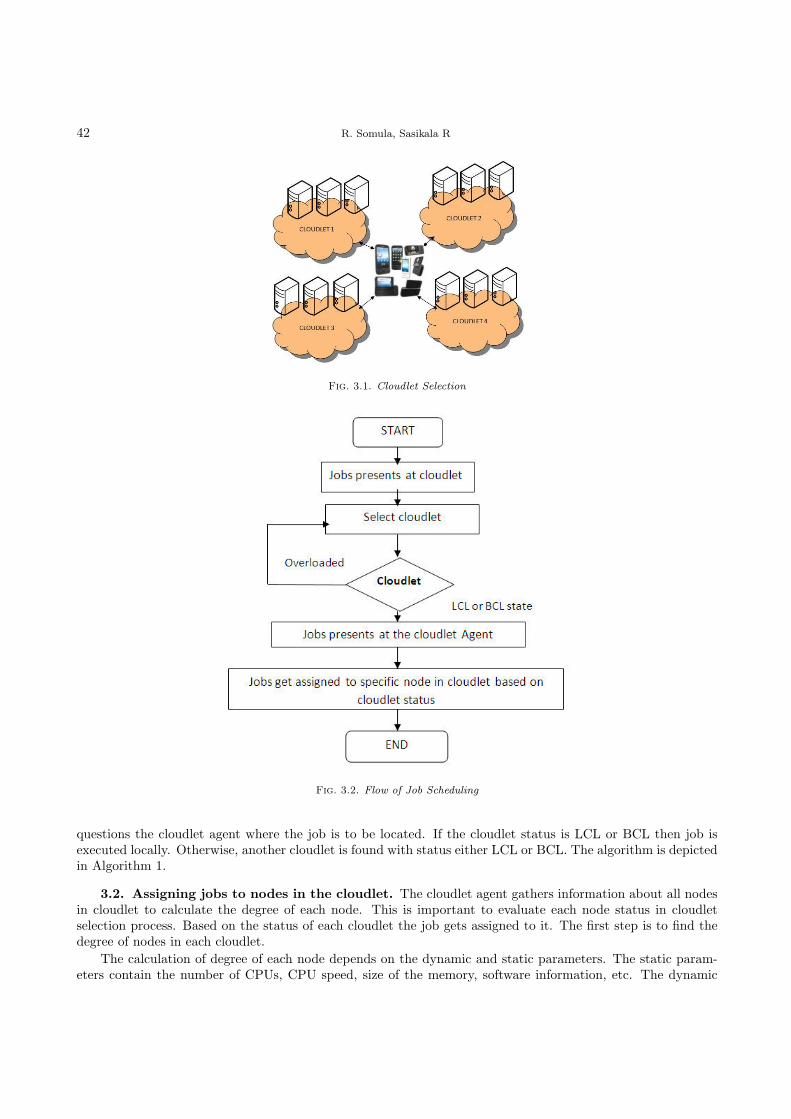
42 R. Somula, Sasikala R
Fig. 3.1. Cloudlet Selection
Fig. 3.2. Flow of Job Scheduling
questions the cloudlet agent where the job is to be located. If the cloudlet status is LCL or BCL then job isexecuted locally. Otherwise, another cloudlet is found with status either LCL or BCL. The algorithm is depictedin Algorithm 1.
3.2. Assigning jobs to nodes in the cloudlet. The cloudlet agent gathers information about all nodesin cloudlet to calculate the degree of each node. This is important to evaluate each node status in cloudletselection process. Based on the status of each cloudlet the job gets assigned to it. The first step is to find thedegree of nodes in each cloudlet.
The calculation of degree of each node depends on the dynamic and static parameters. The static param-eters contain the number of CPUs, CPU speed, size of the memory, software information, etc. The dynamic

Round Robin with Load Degree: An Algorithm for Optimal Cloudlet Discovery in Mobile Cloud Computing 43
Fig. 3.3. Cloudlet Management Architecture
Algorithm 1 Efficient Cloudlet Finding
1: begin
2: while job do
3: SearchPerfectCloudlet (job)4: if cloudlet State=LCL || Cloudlet State=BCL then
5: Send Job to Cloudlet6: else
7: Search for another Cloudlet;8: end if
9: end while
10: end
parameters contain data about usage ratios of CPU, memory, speed, network bandwidth, etc. The evaluationof load degree with different parameters is depicted in the following section.
The cloudlet Load degree values are input to the cloudlet agents for creating tables. Each cloudlet in mobilecloud computing maintains an agent that decides the status of the cloudlet based on values available in thetable. The table updating is done at particular periodic time T . When jobs arrives at cloudlet, the cloudletagent assigns the jobs to a particular node in cloudlet based on cloudlet load status. The cloudlet agent assignsjobs to another cloudlet if cloudlet is not having sufficient resources to handle the incoming jobs.
4. Cloudlet selection with load balancing algorithm. A load balancing mechanism is used to improvethe performance of mobile application by selecting resourceful cloudlet. There is no efficient load strategy tosatisfy all mobile users problems. Each load strategy has its own advantage in specific area. Multiple loadbalancing methods have been developed to solve the existing problem and improve existing solutions. In ourmodel, the load strategy method is changed according to the system status information. System informationcan always be changed based on the load balance method that has been adapted. In this model, simple methodscan be used for LCL state with complex method for BCL. This model mainly aims to select resourceful cloudletto reduce waiting time and improve the performance. An enhanced round robin method is used for LCL whileBCL uses game theory based load balancing method.
4.1. Load Balancing for LCL. When the cloudlet load status is LCL, the nodes in cloudlet are re-sourceful for handling the arriving jobs. Then the cloudlet processes the arriving jobs as fast as possible andalso a simple algorithm is used for scheduling different jobs to nodes. There are many simplest algorithms for

44 R. Somula, Sasikala R
Algorithm 2 Calculation of Load Degree
Step 1: Let the load parameter set B = {B1, B2, B3, . . . , Bm} with each Bi(1 ≤ i ≤ m,B ∈ [0, 1]) theparameter inside set can be static (or) dynamic. M denotes number of parameters.Step 2: Evaluate load degree of node as follows:
Load degree(N) =
m∑
i=1
AiBi
Ai(∑N
i=1Ai = 1) is representing weights of the jobs, it may differ every time. N represents current cloudlet.
Step 3: Calculate the size of the cloudlet from the node degree statistics with the formula
Load degreeavg(N) =
∑N
i=1Load degree(Ni)
n
The threshold Load degreehigh is applicable for various situations based on value of step 3. Where N isnumber of nodes in cloudlet.Step 4: The Cloudlet can be classified into three states as follows:LCL (Low loaded cloudlet): when there is no job to be processed then cloudlet turns to be LCL state.
Load degree(N) = 0
BCL (Balanced cloudlet): when a cloudlet is neither LCL nor OCL, then cloudlet turns to be BCL state.
0 < Load degree(N) = 0 ≤ Load degreehigh
OCL (Overloaded cloudlet): when cloudlet nodes are busy and unable to process incoming jobs then cloudletturns to be OCL state
Load degreehigh < Load degree(N)
scheduling arriving jobs such as round robin algorithm, weighted round robin algorithm, dynamic round robinalgorithm [18]. The Round robin (RR) scheduling strategy is the simplest algorithm for allocating jobs to theservers. RR will send all incoming jobs to queue inside the server but not the main status of each connection.RR scheduling methods consider every node in cloudlet equally so that equal chance is given for every node incloudlet to be chosen. However, in a cloudlet each node differs with respect to configuration and performance.RR can be improved by assigning arriving jobs based on load degree of each node. The incoming jobs getstored into the circular queue. The system goes through the queue over and over. Each cloudlet in public cloudmaintains a table for the load status of the nodes, based on which the nodes get placed in the table from lowload to high load. The order of the nodes in table will be changed based on status of the load status table.However, the inconsistency problem has been taken between read and write at refresh interval T . The jobskeep on arriving at cloudlet manger when load balancing table is being refreshed. This makes wrong cloudletselection and wrong order of cloudlets in the table. Since the table will have old data after getting refreshed,inconsistency problem will lead the arriving jobs to get assigned to wrong node in cloudlet. To address thisproblem, the cloudlet manager should maintain two load refresh tables: Table 1 and Table 2. A label calledread or write can be assigned to each table through flag. The read table contains information of load of thenodes in cloudlet which can be used by improved round robin based on load degree evolution. The write tablewill be updated with new load information. One table provides exact location of the node in the queue andother table is getting written with new information of the nodes. Both read and write labels will be exchangedto avoid inconsistency problem. Figure 4.1 sketches the inconsistency problem to be addressed by read andwrite tables.
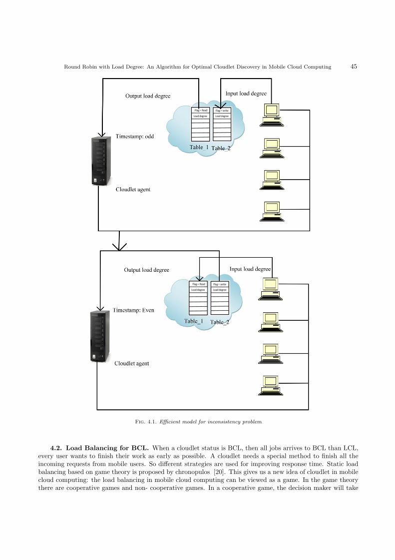
Round Robin with Load Degree: An Algorithm for Optimal Cloudlet Discovery in Mobile Cloud Computing 45
Fig. 4.1. Efficient model for inconsistency problem
4.2. Load Balancing for BCL. When a cloudlet status is BCL, then all jobs arrives to BCL than LCL,every user wants to finish their work as early as possible. A cloudlet needs a special method to finish all theincoming requests from mobile users. So different strategies are used for improving response time. Static loadbalancing based on game theory is proposed by chronopulos [20]. This gives us a new idea of cloudlet in mobilecloud computing: the load balancing in mobile cloud computing can be viewed as a game. In the game theorythere are cooperative games and non- cooperative games. In a cooperative game, the decision maker will take

46 R. Somula, Sasikala R
decision by discussing with other player or comparing each node with each other. In a non- cooperative gamethe decision is taken for his own benefit and the other players in the game will take their own decision. Thesystem will reach to Nash equilibrium where each player will make his/her own optimized decision and no playergets benefited by changing his or her own plan, while remaining players decisions are unchanged.
The game theory has been proposed by many studies to solve various problems and was adapted by differentareas. It is mainly introduced for distributed computing and later it has been popular in cloud computing too.A dynamic load balancing based on game theory is proposed by Aote and Khara [3]. In this method, usersbeing decision makers in non-cooperative game. Mobile cloud computing is integrated with multiple technolo-gies, networking, mobile computing and cloud computing. Mobile cloud computing is also viewed as distributedcomputing because this MCC technology is integrated with cloud computing. So the load balancing algorithmcan be viewed as a non-cooperative game. The players in the game are nodes and jobs. For instance there are’n’ nodes in current cloudlet with ’m’ arriving jobs. The following define this process:
βi: Each node processing ability, i= 1, 2, . . . , n
φj : Each job execution time
φ :∑N
j=1φj : total time of the entire cloudlet for processing φ <
∑n
i=1βi
Fji: Job j get assigned to node (∑n
i=1Fji) and 0 ≤ Fji ≤ 1
Finding appropriate value Fji is an important step. Grosu et al. [12] has proposed a model called best replyby using this model to evaluate Fji for each node with a greedy algorithm. The procedure will produce a Nashequilibrium to reduce response time of each job. The balancing mechanism changes according to the systemstatus information. Figure 4.2 depicts the proposed model.
Fig. 4.2. Proposed cloudlet selection model
4.3. Extended Round Robin Algorithm. We use the Algorithm 3 to find optimal cloudlet to processtasks coming from mobile users in MCC environment.
5. Performance Evaluation. In this section we describe how the proposed algorithm performs in variouswork loaded environments using cloudlets. The computing performance of proposed algorithm is compared with
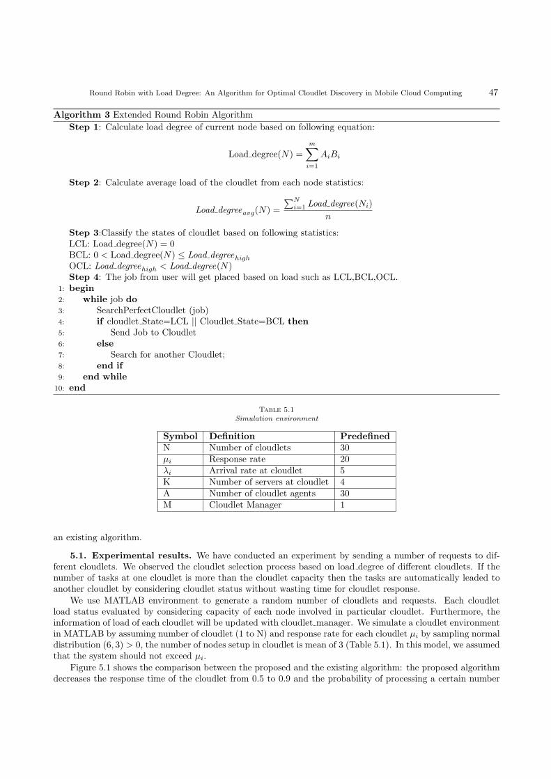
Round Robin with Load Degree: An Algorithm for Optimal Cloudlet Discovery in Mobile Cloud Computing 47
Algorithm 3 Extended Round Robin Algorithm
Step 1: Calculate load degree of current node based on following equation:
Load degree(N) =m∑
i=1
AiBi
Step 2: Calculate average load of the cloudlet from each node statistics:
Load degreeavg(N) =
∑N
i=1Load degree(Ni)
n
Step 3:Classify the states of cloudlet based on following statistics:LCL: Load degree(N) = 0BCL: 0 < Load degree(N) ≤ Load degreehighOCL: Load degreehigh < Load degree(N)Step 4: The job from user will get placed based on load such as LCL,BCL,OCL.
1: begin
2: while job do
3: SearchPerfectCloudlet (job)4: if cloudlet State=LCL || Cloudlet State=BCL then
5: Send Job to Cloudlet6: else
7: Search for another Cloudlet;8: end if
9: end while
10: end
Table 5.1
Simulation environment
Symbol Definition Predefined
N Number of cloudlets 30µi Response rate 20λi Arrival rate at cloudlet 5K Number of servers at cloudlet 4A Number of cloudlet agents 30M Cloudlet Manager 1
an existing algorithm.
5.1. Experimental results. We have conducted an experiment by sending a number of requests to dif-ferent cloudlets. We observed the cloudlet selection process based on load degree of different cloudlets. If thenumber of tasks at one cloudlet is more than the cloudlet capacity then the tasks are automatically leaded toanother cloudlet by considering cloudlet status without wasting time for cloudlet response.
We use MATLAB environment to generate a random number of cloudlets and requests. Each cloudletload status evaluated by considering capacity of each node involved in particular cloudlet. Furthermore, theinformation of load of each cloudlet will be updated with cloudlet manager. We simulate a cloudlet environmentin MATLAB by assuming number of cloudlet (1 to N) and response rate for each cloudlet µi by sampling normaldistribution (6, 3) > 0, the number of nodes setup in cloudlet is mean of 3 (Table 5.1). In this model, we assumedthat the system should not exceed µi.
Figure 5.1 shows the comparison between the proposed and the existing algorithm: the proposed algorithmdecreases the response time of the cloudlet from 0.5 to 0.9 and the probability of processing a certain number
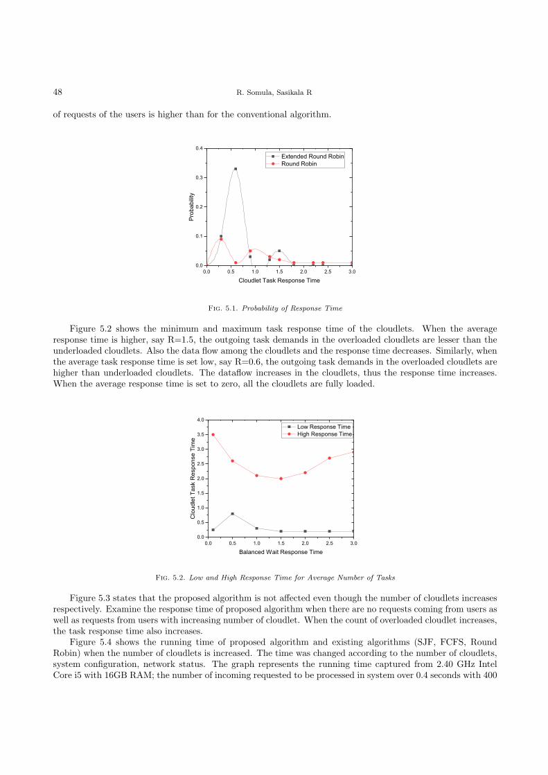
48 R. Somula, Sasikala R
of requests of the users is higher than for the conventional algorithm.
0.0 0.5 1.0 1.5 2.0 2.5 3.00.0
0.1
0.2
0.3
0.4
Prob
abilit
y
Cloudlet Task Response Time
Extended Round Robin Round Robin
Fig. 5.1. Probability of Response Time
Figure 5.2 shows the minimum and maximum task response time of the cloudlets. When the averageresponse time is higher, say R=1.5, the outgoing task demands in the overloaded cloudlets are lesser than theunderloaded cloudlets. Also the data flow among the cloudlets and the response time decreases. Similarly, whenthe average task response time is set low, say R=0.6, the outgoing task demands in the overloaded cloudlets arehigher than underloaded cloudlets. The dataflow increases in the cloudlets, thus the response time increases.When the average response time is set to zero, all the cloudlets are fully loaded.
0.0 0.5 1.0 1.5 2.0 2.5 3.00.0
0.5
1.0
1.5
2.0
2.5
3.0
3.5
4.0
Clo
udle
t Tas
k R
espo
nse
Tim
e
Balanced Wait Response Time
Low Response Time High Response Time
Fig. 5.2. Low and High Response Time for Average Number of Tasks
Figure 5.3 states that the proposed algorithm is not affected even though the number of cloudlets increasesrespectively. Examine the response time of proposed algorithm when there are no requests coming from users aswell as requests from users with increasing number of cloudlet. When the count of overloaded cloudlet increases,the task response time also increases.
Figure 5.4 shows the running time of proposed algorithm and existing algorithms (SJF, FCFS, RoundRobin) when the number of cloudlets is increased. The time was changed according to the number of cloudlets,system configuration, network status. The graph represents the running time captured from 2.40 GHz IntelCore i5 with 16GB RAM; the number of incoming requested to be processed in system over 0.4 seconds with 400

Round Robin with Load Degree: An Algorithm for Optimal Cloudlet Discovery in Mobile Cloud Computing 49
0 50 100 150 2000.5
1.0
1.5
2.0
2.5
3.0
3.5
4.0
Max
imum
Wai
t Tim
e of
Arri
val J
obs
Number of Cloudlets
Proposed algorithm SJF FCFS Round Robin
Fig. 5.3. Delay for Arrival Jobs with Different Cloudlets
cloudlets. The table updating is done at particular periodic time T when jobs arrives at cloudlet: the cloudletagent assigns jobs to particular nodes in cloudlet based on cloudlet load status.
0 50 100 150 2000
50
100
150
200
250
300
350
Run
ning
Tim
e(M
S)
Number of Cloudlets
Proposed Algorithm SJF FCFS Round Robin
Fig. 5.4. Running time of proposed algorithm on number of cloudlets
Figure 5.5 shows the cloudlet task response time with and without the proposed algorithm in a staticnetwork. As graph shows, the number of incoming jobs increases, while the task response time also increasesunder normal distribution. As can be seen, the cloudlet response time can be different from the existingalgorithm. The execution time includes transferring time and processing time. If the number of requestscomming from the users increases then the performance of existing algorithms is decreasing.
Figure 5.6 shows the cloudlet task response time for proposed method, SJF, FCFS and RR algorithms in astatic network. The X-axis represents the cloudlet response time and the y-axis represents the cloudlet arrivalrate. As graph shows, the Proposed Method is efficient in comparison with the other three existing algorithms.
6. Conclusion and Future work. This paper proposed a novel conceptual framework which is mainlyfocusing on selection of distributed resourceful cloudlet in a public cloud with the help of a load balancingalgorithm. The Cloudlet manager and Cloudlet agent are responsible for scheduling the arriving jobs in the
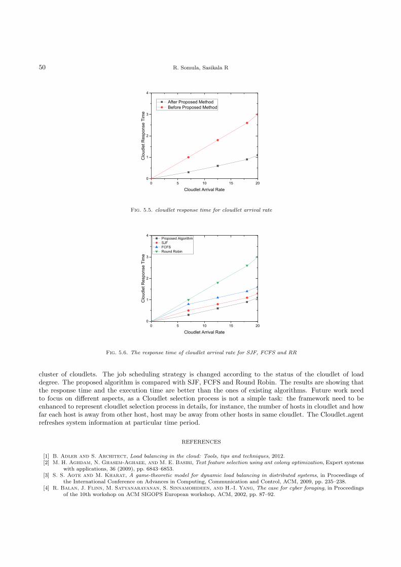
50 R. Somula, Sasikala R
0 5 10 15 200
1
2
3
4
Clo
udle
t Res
pons
e Ti
me
Cloudlet Arrival Rate
After Proposed Method Before Proposed Method
Fig. 5.5. cloudlet response time for cloudlet arrival rate
0 5 10 15 200
1
2
3
4
Clo
udle
t Res
pons
e Ti
me
Cloudlet Arrival Rate
Proposed Algorithm SJF FCFS Round Robin
Fig. 5.6. The response time of cloudlet arrival rate for SJF, FCFS and RR
cluster of cloudlets. The job scheduling strategy is changed according to the status of the cloudlet of loaddegree. The proposed algorithm is compared with SJF, FCFS and Round Robin. The results are showing thatthe response time and the execution time are better than the ones of existing algorithms. Future work needto focus on different aspects, as a Cloudlet selection process is not a simple task: the framework need to beenhanced to represent cloudlet selection process in details, for instance, the number of hosts in cloudlet and howfar each host is away from other host, host may be away from other hosts in same cloudlet. The Cloudlet agentrefreshes system information at particular time period.
REFERENCES
[1] B. Adler and S. Architect, Load balancing in the cloud: Tools, tips and techniques, 2012.[2] M. H. Aghdam, N. Ghasem-Aghaee, and M. E. Basiri, Text feature selection using ant colony optimization, Expert systems
with applications, 36 (2009), pp. 6843–6853.[3] S. S. Aote and M. Kharat, A game-theoretic model for dynamic load balancing in distributed systems, in Proceedings of
the International Conference on Advances in Computing, Communication and Control, ACM, 2009, pp. 235–238.[4] R. Balan, J. Flinn, M. Satyanarayanan, S. Sinnamohideen, and H.-I. Yang, The case for cyber foraging, in Proceedings
of the 10th workshop on ACM SIGOPS European workshop, ACM, 2002, pp. 87–92.

Round Robin with Load Degree: An Algorithm for Optimal Cloudlet Discovery in Mobile Cloud Computing 51
[5] N. Bobroff, A. Kochut, and K. Beaty, Dynamic placement of virtual machines for managing sla violations, in IntegratedNetwork Management, 2007. IM’07. 10th IFIP/IEEE International Symposium on, IEEE, 2007, pp. 119–128.
[6] V. Cardellini, V. D. N. Persone, V. Di Valerio, F. Facchinei, V. Grassi, F. L. Presti, and V. Piccialli, A game-
theoretic approach to computation offloading in mobile cloud computing, Mathematical Programming, 157 (2016), pp. 421–449.
[7] B.-G. Chun, S. Ihm, P. Maniatis, M. Naik, and A. Patti, Clonecloud: elastic execution between mobile device and cloud,in Proceedings of the sixth conference on Computer systems, ACM, 2011, pp. 301–314.
[8] E. Cuervo, A. Balasubramanian, D.-k. Cho, A. Wolman, S. Saroiu, R. Chandra, and P. Bahl, Maui: making smart-
phones last longer with code offload, in Proceedings of the 8th international conference on Mobile systems, applications,and services, ACM, 2010, pp. 49–62.
[9] H. T. Dinh, C. Lee, D. Niyato, and P. Wang, A survey of mobile cloud computing: architecture, applications, and
approaches, Wireless communications and mobile computing, 13 (2013), pp. 1587–1611.[10] E. Gelenbe, R. Lent, and M. Douratsos, Choosing a local or remote cloud, in Network Cloud Computing and Applications
(NCCA), 2012 Second Symposium on, IEEE, 2012, pp. 25–30.[11] L. Gkatzikis and I. Koutsopoulos, Migrate or not? exploiting dynamic task migration in mobile cloud computing systems,
IEEE Wireless Communications, 20 (2013), pp. 24–32.[12] D. Grosu, A. T. Chronopoulos, and M.-Y. Leung, Load balancing in distributed systems: An approach using cooperative
games, in Parallel and Distributed Processing Symposium., Proceedings International, IPDPS 2002, Abstracts and CD-ROM, IEEE, 2001, pp. 10–pp.
[13] J. Heo, K. Terada, M. Toyama, S. Kurumatani, and E. Y. Chen, User demand prediction from application usage
pattern in virtual smartphone, in Cloud Computing Technology and Science (CloudCom), 2010 IEEE Second InternationalConference on, IEEE, 2010, pp. 449–455.
[14] D. T. Hoang, D. Niyato, and P. Wang, Optimal admission control policy for mobile cloud computing hotspot with cloudlet,in Wireless Communications and Networking Conference (WCNC), 2012 IEEE, IEEE, 2012, pp. 3145–3149.
[15] Y. Jararweh, F. Ababneh, A. Khreishah, F. Dosari, et al., Scalable cloudlet-based mobile computing model, ProcediaComputer Science, 34 (2014), pp. 434–441.
[16] L. Kleinrock, Queueing systems, volume 2: Computer applications, vol. 66, wiley New York, 1976.[17] S. Kosta, A. Aucinas, P. Hui, R. Mortier, and X. Zhang, Thinkair: Dynamic resource allocation and parallel execution
in the cloud for mobile code offloading, in Infocom, 2012 Proceedings IEEE, IEEE, 2012, pp. 945–953.[18] D. MacVittie, Intro to load balancing for developersthe algorithms, 2012.[19] N. Palaniappan and S. Ramasamy, A survey on procedures dealing with mobile offloading schemes, 7 (2017), p. 178.[20] S. Penmatsa and A. T. Chronopoulos, Game-theoretic static load balancing for distributed systems, Journal of Parallel
and Distributed Computing, 71 (2011), pp. 537–555.[21] M. Randles, D. Lamb, and A. Taleb-Bendiab, A comparative study into distributed load balancing algorithms for cloud
computing, in Advanced Information Networking and Applications Workshops (WAINA), 2010 IEEE 24th InternationalConference on, IEEE, 2010, pp. 551–556.
[22] Z. Sanaei, S. Abolfazli, A. Gani, and R. Buyya, Heterogeneity in mobile cloud computing: taxonomy and open challenges,IEEE Communications Surveys & Tutorials, 16 (2014), pp. 369–392.
[23] M. Satyanarayanan, Pervasive computing: Vision and challenges, IEEE Personal communications, 8 (2001), pp. 10–17.[24] M. Satyanarayanan, P. Bahl, R. Caceres, and N. Davies, The case for vm-based cloudlets in mobile computing, IEEE
pervasive Computing, 8 (2009).[25] N. G. Shivaratri, P. Krueger, and M. Singhal, Load distributing for locally distributed systems, Computer, 25 (1992),
pp. 33–44.[26] H. N. Van, F. D. Tran, and J.-M. Menaud, Sla-aware virtual resource management for cloud infrastructures, in Computer
and Information Technology, 2009. CIT’09. Ninth IEEE International Conference on, vol. 1, IEEE, 2009, pp. 357–362.[27] T. Verbelen, P. Simoens, F. De Turck, and B. Dhoedt, Cloudlets: Bringing the cloud to the mobile user, in Proceedings
of the third ACM workshop on Mobile cloud computing and services, ACM, 2012, pp. 29–36.[28] Q. Xia, W. Liang, and W. Xu, Throughput maximization for online request admissions in mobile cloudlets, in Local
Computer Networks (LCN), 2013 IEEE 38th Conference on, IEEE, 2013, pp. 589–596.[29] Q. Xia, W. Liang, Z. Xu, and B. Zhou, Online algorithms for location-aware task offloading in two-tiered mobile cloud
environments, in Utility and Cloud Computing (UCC), 2014 IEEE/ACM 7th International Conference on, IEEE, 2014,pp. 109–116.
[30] G. Xu, J. Pang, and X. Fu, A load balancing model based on cloud partitioning for the public cloud, Tsinghua Science andTechnology, 18 (2013), pp. 34–39.
[31] K. Yang, S. Ou, and H.-H. Chen, On effective offloading services for resource-constrained mobile devices running heavier
mobile internet applications, IEEE communications magazine, 46 (2008).
Edited by: Dana PetcuReceived: Sep 23, 2017Accepted: Feb 16, 2018

Scalable Computing: Practice and Experience
Volume 19, Number 1, pp. 53–67. http://www.scpe.org
DOI 10.12694/scpe.v19i1.1393ISSN 1895-1767c⃝ 2018 SCPE
AUTOADMIN: AUTOMATIC AND DYNAMIC RESOURCE RESERVATION ADMISSION
CONTROL IN HADOOP YARN CLUSTERS
ZHENGYU YANG, JANKI BHIMANI, YI YAO, CHO-HSIEN LIN∗, JIAYIN WANG†, NINGFANG MI‡, AND BO SHENG§
Abstract. Hadoop YARN is an Apache Software Foundation’s open project that provides a resource management frameworkfor large scale parallel data processing, such as MapReduce jobs. Fair scheduler is a dispatcher which has been widely used in YARNto assign resources fairly and equally to applications. However, there exists a problem of the Fair scheduler when the resourcerequisition of applications is beyond the amount that the cluster can provide. In such a case, the YARN system will be haltedif all resources are occupied by ApplicationMasters, a special task of each job that negotiates resources for processing tasks andcoordinates job execution. To solve this problem, we propose an automatic and dynamic admission control mechanism to preventthe ceasing situation happened when the requested amount of resources exceeds the cluster’s resource capacity, and dynamicallyreserve resources for processing tasks in order to obtain good performance, e.g., reducing makespans of MapReduce jobs. Aftercollecting resource usage information of each work node, our mechanism dynamically predicts the amount of reserved resources forprocessing tasks and automatically controls running jobs based on the prediction. We implement the new mechanism in HadoopYARN and evaluate it with representative MapReduce benchmarks. The experimental results show the effectiveness and robustnessof this mechanism under both homogeneous and heterogeneous workloads.
Key words: Cloud Computing, MapReduce, Hadoop, YARN, Scheduling, Resource Management, Admission Control, BigData, Scalable Computing, Cluster Computing
AMS subject classifications. 68M14, 68P05
1. Introduction. Large scale data analysis is of great importance in a variety of research and industrialareas during the age of data explosion and cloud computing. MapReduce [11] becomes one of the most popularprograming paradigms in recent years. Its open source implementation Hadoop [5] has been widely adopted asthe primary platform for parallel data processing [1]. Recently, the Hadoop MapReduce ecosystem is evolvinginto its next generation, called Hadoop YARN (Yet Another Resource Negotiator) [19], which adopts fine-grainedresource management for job scheduling.
The architecture of YARN is shown in Figure 1.1. Similar to the traditional Hadoop, a YARN systemoften consists of one centralized manager node running the ResourceManager (RM) daemon and multiple worknodes running the NodeManager (NM) daemons. However, there are two major differences between YARN andtraditional Hadoop. First, the RM in YARN no longer monitors and coordinates job execution as the JobTrackerof traditional Hadoop does. Alternatively, an ApplicationMaster(AM) is generated for each application in YARNto coordinate all processing tasks (e.g., map/reduce tasks) from that application. Therefore, the RM in YARNis more scalable than the JobTracker in traditional Hadoop. Secondly, YARN abandons the previous coarsegrained slot configuration used by TaskTrackers in traditional Hadoop. Instead, NMs in YARN consider fine-grained resource management for managing various resources. e.g., CPU and memory, in the cluster.
On the other hand, YARN uses the same scheduling mechanisms as traditional Hadoop and supports theexisting scheduling policies (such as FIFO, Fair and Capacity) as the default schedulers. However, we found thata resource (or “container”) starvation problem exists in the present YARN scheduling under Fair and Capacity.As mentioned above, for each application in YARN, an ApplicationMaster is first generated to coordinate itsprocessing tasks. Such an ApplicationMaster is indeed a special task in the YARN system, which has a higherpriority to get resources (or containers) and stays alive without releasing resources till all processing tasks of thatapplication finish. Consequently, when the amount of concurrently running jobs becomes too high, for example,a burst of jobs arrived, it is highly likely that system resources are fully occupied by ApplicationMasters of
∗ Department of Electrical & Computer Engineering, Northeastern University, 360 Huntington Ave., Boston, MA, USA, 02115([email protected], [email protected], [email protected], [email protected]).
†Computer Science Department, Montclair State University, 1 Normal Ave, Montclair, NJ, USA, 07043 ([email protected])‡ Department of Electrical & Computer Engineering, Northeastern University, 360 Huntington Ave., Boston, MA, USA, 02115
([email protected]).§ Deptartment of Computer Science, University of Massachusetts Boston, 100 Morrissey Boulevard, Boston, MA, USA 02125
53
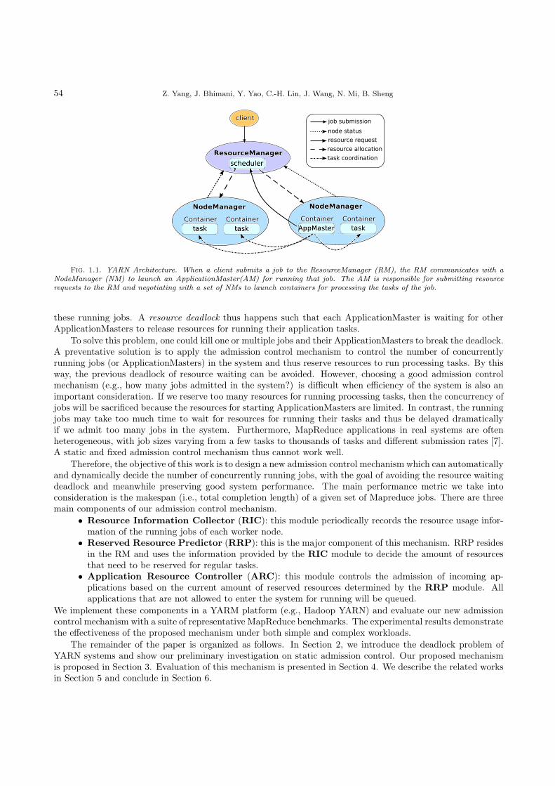
54 Z. Yang, J. Bhimani, Y. Yao, C.-H. Lin, J. Wang, N. Mi, B. Sheng
ResourceManager
NodeManager
Container
client
Container
NodeManager
Container Container
job submission
node status
resource request
resource allocation
task coordination
Fig. 1.1. YARN Architecture. When a client submits a job to the ResourceManager (RM), the RM communicates with aNodeManager (NM) to launch an ApplicationMaster(AM) for running that job. The AM is responsible for submitting resourcerequests to the RM and negotiating with a set of NMs to launch containers for processing the tasks of the job.
these running jobs. A resource deadlock thus happens such that each ApplicationMaster is waiting for otherApplicationMasters to release resources for running their application tasks.
To solve this problem, one could kill one or multiple jobs and their ApplicationMasters to break the deadlock.A preventative solution is to apply the admission control mechanism to control the number of concurrentlyrunning jobs (or ApplicationMasters) in the system and thus reserve resources to run processing tasks. By thisway, the previous deadlock of resource waiting can be avoided. However, choosing a good admission controlmechanism (e.g., how many jobs admitted in the system?) is difficult when efficiency of the system is also animportant consideration. If we reserve too many resources for running processing tasks, then the concurrency ofjobs will be sacrificed because the resources for starting ApplicationMasters are limited. In contrast, the runningjobs may take too much time to wait for resources for running their tasks and thus be delayed dramaticallyif we admit too many jobs in the system. Furthermore, MapReduce applications in real systems are oftenheterogeneous, with job sizes varying from a few tasks to thousands of tasks and different submission rates [7].A static and fixed admission control mechanism thus cannot work well.
Therefore, the objective of this work is to design a new admission control mechanism which can automaticallyand dynamically decide the number of concurrently running jobs, with the goal of avoiding the resource waitingdeadlock and meanwhile preserving good system performance. The main performance metric we take intoconsideration is the makespan (i.e., total completion length) of a given set of Mapreduce jobs. There are threemain components of our admission control mechanism.
• Resource Information Collector (RIC): this module periodically records the resource usage infor-mation of the running jobs of each worker node.
• Reserved Resource Predictor (RRP): this is the major component of this mechanism. RRP residesin the RM and uses the information provided by the RIC module to decide the amount of resourcesthat need to be reserved for regular tasks.
• Application Resource Controller (ARC): this module controls the admission of incoming ap-plications based on the current amount of reserved resources determined by the RRP module. Allapplications that are not allowed to enter the system for running will be queued.
We implement these components in a YARM platform (e.g., Hadoop YARN) and evaluate our new admissioncontrol mechanism with a suite of representative MapReduce benchmarks. The experimental results demonstratethe effectiveness of the proposed mechanism under both simple and complex workloads.
The remainder of the paper is organized as follows. In Section 2, we introduce the deadlock problem ofYARN systems and show our preliminary investigation on static admission control. Our proposed mechanismis proposed in Section 3. Evaluation of this mechanism is presented in Section 4. We describe the related worksin Section 5 and conclude in Section 6.

AutoAdmin: Automatic and Dynamic Resource Reservation Admission Control in Hadoop YARN Clusters 55
2. Motivation.
2.1. Background. In a YARN system, each application needs to specify the resource requirements of alltheir tasks, such as ApplicationMasters, map tasks and reduce tasks. The resource requirement is a bundle ofphysical resources with the format as <2 CPU, 1GB RAM>, for example. Then, a task from that applicationwill only be executed in a container whose resource capacity (e.g., 2 CPU and 1GB RAM) is equal to thattask’s resource demand. Meanwhile, the NodeManager (NM) keeps monitoring the actual resource usage ofthat container and could kill that container if the actual usage exceeds the granted resource amount.
The ResourceManager (RM) acts as a central arbitrator, dispatching available containers to various com-peting applications in light of each application’s resource demand and the scheduling policy. NMs residing inthe work machines (i.e., slave nodes) associate with the RM to manage the resource; they periodically reportthe information of resource and containers usage to the RM through the heartbeat message in YARN. Thescheduler in the RM then schedules the queuing jobs based on the waiting resource requests of applications andthe current residual resource amount on each slave node.
When an application is submitted, the RM needs to first allocate resources for launching the Application-Master container on a work node according to the resource requirement specified by the client. The launchedAM will then send resource requests for processing remaining tasks of that application to the RM. The RMresponses with resource allocations on NMs and the AM then communicate with the NMs for launching con-tainers and executing tasks. The AM is also responsible for monitoring and coordinating the execution of otherprocessing tasks, e.g., re-submitting failed tasks, gradually submitting reduce tasks according to the progress ofmap tasks, etc.. Therefore, the AM only terminates and releases the resources its container occupies after allthe remaining tasks of its application are finished.
Moreover, the AM is the head of a job and it must be launched firstly when processing the job. SinceAM needs to harness some resource to running the job’s tasks, it will issue requests to RM for allocating theTask Container (TC) to process the tasks. While RM accepts the requests then it will response to AM thatwhich nodes have the available resource. The AM then continuously negotiates with the NMs of those nodesto running the tasks. Finally, while all the tasks are processed the AM can be finished and the RM will releasethe AMC. In conclusion, the RM and NM starts running when the YARN system is set up; however, the AMlaunched upon a container is based on the condition that a job is submitted to the RM and the RM accepts toprocessing it; then, the AM can start its negotiating mission, relative state [17] is as Fig. 2.1.
2.2. The Deadlock Problem of Fair Scheduler in YARN. Since an ApplicationMaster is the firstlaunched task of each job and will not release its resource until the associated job finishes, the number of AMtasks running in a YARN system is always equal to the number of concurrently running jobs. It is not a problemif a small amount of jobs are concurrently running in the system. However, it is possible that these AMs useup most or even all of the resources during a busy period, for example, when a large amount of users submitmany ad-hoc MapReduce query jobs. In such a case, the YARN system faces a deadlock problem, i.e., noneof these AMs could get resources for running their map/reduce tasks. Consequently, overall efficiency of theYARN system is severely degraded because the AMs are occupying most resources yet waiting for others torelease resources.
Therefore, our goal in this work is to design a new mechanism that can automatically control the resourcereservation in the YARN system such that the deadlock problem can be avoided even under busy conditions whenresource demands of AMs exceed the entire cluster capacity. Moreover, this new mechanism can dynamicallyadjust the strategy for resource reservation according to the present workloads in order to improve the efficiencyof the YARN system, e.g., minimizing the makespan (i.e., the overall completion length) of a set of MapReducejobs.
2.3. Preliminary Investigations. The basic solution of preventing the deadlock situation is to reserve afixed amount of resources for non-AM processing tasks. However, as we discussed before, the system performancecould be degraded if the reservation number is not carefully chosen. We first modify the Fair scheduler to supportthe static resource reservation and investigate the impact of resource reservation on the performance. Two setsof experiments are conducted to evaluate the performance of resource reservations. For the sake of simplicity,we only consider the cpu resource in these experiments (i.e., all jobs are cpu intensive). The YARN cluster we
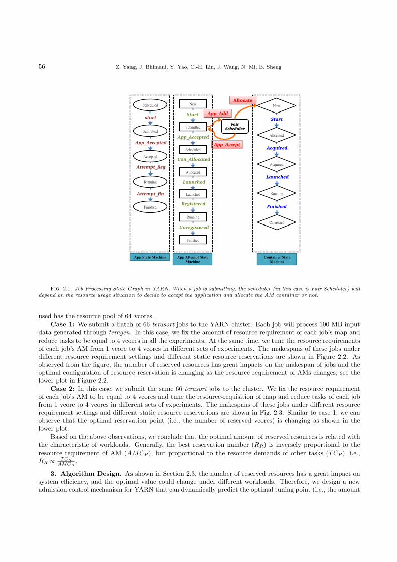
56 Z. Yang, J. Bhimani, Y. Yao, C.-H. Lin, J. Wang, N. Mi, B. Sheng
App_Accept
A
F
N w
start
A
L
F
Fair Scheduler
N w
A
A
C
App_Accepted
Attempt_Reg
Attempt_fin
App_Accepted
Con_Allocated
Launched
Registered
Unregistered
Start
Acquired
Launched
Finished
Start
App State Machine App Attempt State
Machine Container State
Machine
App_Add
Allocate
Fig. 2.1. Job Processing State Graph in YARN. When a job is submitting, the scheduler (in this case is Fair Scheduler) willdepend on the resource usage situation to decide to accept the application and allocate the AM container or not.
used has the resource pool of 64 vcores.Case 1: We submit a batch of 66 terasort jobs to the YARN cluster. Each job will process 100 MB input
data generated through teragen. In this case, we fix the amount of resource requirement of each job’s map andreduce tasks to be equal to 4 vcores in all the experiments. At the same time, we tune the resource requirementsof each job’s AM from 1 vcore to 4 vcores in different sets of experiments. The makespans of these jobs underdifferent resource requirement settings and different static resource reservations are shown in Figure 2.2. Asobserved from the figure, the number of reserved resources has great impacts on the makespan of jobs and theoptimal configuration of resource reservation is changing as the resource requirement of AMs changes, see thelower plot in Figure 2.2.
Case 2: In this case, we submit the same 66 terasort jobs to the cluster. We fix the resource requirementof each job’s AM to be equal to 4 vcores and tune the resource-requisition of map and reduce tasks of each jobfrom 1 vcore to 4 vcores in different sets of experiments. The makespans of these jobs under different resourcerequirement settings and different static resource reservations are shown in Fig. 2.3. Similar to case 1, we canobserve that the optimal reservation point (i.e., the number of reserved vcores) is changing as shown in thelower plot.
Based on the above observations, we conclude that the optimal amount of reserved resources is related withthe characteristic of workloads. Generally, the best reservation number (RR) is inversely proportional to theresource requirement of AM (AMCR), but proportional to the resource demands of other tasks (TCR), i.e.,RR ∝
TCR
AMCR
.
3. Algorithm Design. As shown in Section 2.3, the number of reserved resources has a great impact onsystem efficiency, and the optimal value could change under different workloads. Therefore, we design a newadmission control mechanism for YARN that can dynamically predict the optimal tuning point (i.e., the amount

AutoAdmin: Automatic and Dynamic Resource Reservation Admission Control in Hadoop YARN Clusters 57
48
40 36
32
0
10
20
30
40
50
60
(1,4) (2,4) (3,4) (4,4)
Resource(Vcore)
(AMCR,TCR)
Minimum Makespan
0
200
400
600
800
1000
1200
1400
1600
20 22 24 26 28 30 32 34 36 38 40 42 44 46 48 50 52 54 56
Tim
e (
s)
Reserved Resource (vcore)
AM=1
AM=2
AM=3
AM=4
Fig. 2.2. Makespans of 66 terasort jobs under different resource requirement settings on AM and different static resourcereservations.
of resources reserved for non-AM tasks) and perform the admission control on incoming YARN jobs. There arethree main components in our mechanism:
• RIC (Resource Information Collector): collect the resource and container’s information from each nodethrough heartbeat messages.
• RRP (Reserved Resource Predictor): decide how many resources should be reserved based on theinformation collected by from RIC.
• ARC (Application Resource Controller): leverage the predicted value of RRP to manipulate an appli-cation’s running.
We will describe the design of these components in details in the following sections.
3.1. Resource Information Collector. The key function of this component is to record the numberof currently running ApplicationMasters and normal processing tasks as well as the resources that have beenoccupied by these two kinds of containers on each worker node. A map data structure is maintained to record theinformation and will be updated through each heartbeat message between NodeManager and ResourceManager.The algorithm of RIC is shown in Alg. 4.
3.2. Reserved Resource Predictor. The purpose of the RRP component is to find out the amountof reserved resources that can not only preserve high throughput of the system but also prevent the deadlockproblem. As shown in Section 2.3, the optimal value of reservation is varying under different workloads.Therefore, the RRP component should be frequently triggered to recalculate the desired reservation level inorder to adapt to dynamic workload changes. The overhead of this component thus becomes a primary concernwhen the workload changes too frequently. In this paper, we propose a simple, heuristic approach to decidean appropriate reservation level according to the information of workload characteristics provided by the RICcomponent.

58 Z. Yang, J. Bhimani, Y. Yao, C.-H. Lin, J. Wang, N. Mi, B. Sheng
0
200
400
600
800
1000
1200
1400
1600
1800
2000
20 22 24 26 28 30 32 34 36 38 40 42 44 46 48 50 52 54 56
Tim
e (
s)
Reserved Resource (vcore)
Task=1
Task=2
Task=3
Task=4
26 24
28
32
0
5
10
15
20
25
30
35
(4,1) (4,2) (4,3) (4,4)
Resource (Vcore)
(AMCR,TCR)
Minimum Makespan
Fig. 2.3. Makespans of 66 terasort jobs under different resource requirement settings on map/reduce tasks and different staticresource reservations.
Algorithm 1: Resource Information Collector
Data:
Number of AM containers in node Ni: NAMCNi;
Number of task containers in node Ni: NTCNi;
Total resource of AMC in node Ni: Total AMCNi;
Total resource of TC in node Ni: Total TCNi;
HashMap that records each node’s AMC information: Map AMC;
HashMap that records each node’s TC information: Map TC;
1 while each node Ni doing NodeUpdate do
2 Record or update Ni: NAMCNiand Total AMCNi
into Map AMC;
3 Record or update Ni: NTCNiand Total TCNi
into Map TC;
4 Update AvgAMCR and AvgTCR;
In Section 2.3, we also find that the optimal amount of reserved resources (RR) seems to be proportional andinversely proportional to the resource requisition of non-AM task’s (TCR) and AM task’s (AMCR) containers,i.e., RR ∝
TCR
AMCR
, under static workloads. To get a more clear understanding of this relationship, we conduct16 sets of experiments. In each set of experiments, we run a batch of jobs with the same resource requirements,i.e., static workloads, repeatedly under different static resource reservations. The optimal resource reservationamounts in terms of makespan are shown in Figure 3.1. We can observe a linear relationship between theoptimal reservation and the resource requirements of AM and tasks of jobs. Thus, we have the function:
RR = CR ·
TCR
AMCR + TCR
, (3.1)
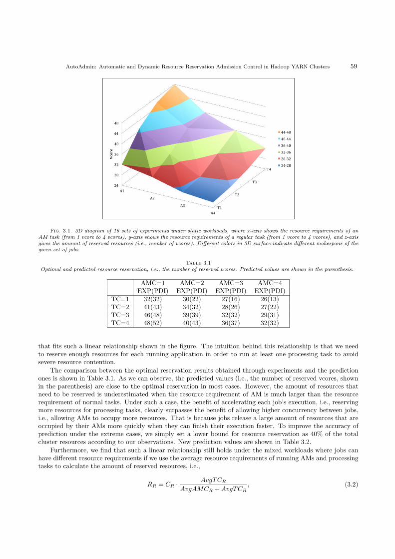
AutoAdmin: Automatic and Dynamic Resource Reservation Admission Control in Hadoop YARN Clusters 59
T1
T2
T3
T4
24
28
32
36
40
44
48
A1
A2
A3
A4
Vcore
44‐48
40‐44
36‐40
32‐36
28‐32
24‐28
Fig. 3.1. 3D diagram of 16 sets of experiments under static workloads, where x-axis shows the resource requirements of anAM task (from 1 vcore to 4 vcores), y-axis shows the resource requirements of a regular task (from 1 vcore to 4 vcores), and z-axisgives the amount of reserved resources (i.e., number of vcores). Different colors in 3D surface indicate different makespans of thegiven set of jobs.
Table 3.1
Optimal and predicted resource reservation, i.e., the number of reserved vcores. Predicted values are shown in the parenthesis.
AMC=1 AMC=2 AMC=3 AMC=4EXP(PDI) EXP(PDI) EXP(PDI) EXP(PDI)
TC=1 32(32) 30(22) 27(16) 26(13)TC=2 41(43) 34(32) 28(26) 27(22)TC=3 46(48) 39(39) 32(32) 29(31)TC=4 48(52) 40(43) 36(37) 32(32)
that fits such a linear relationship shown in the figure. The intuition behind this relationship is that we needto reserve enough resources for each running application in order to run at least one processing task to avoidsevere resource contention.
The comparison between the optimal reservation results obtained through experiments and the predictionones is shown in Table 3.1. As we can observe, the predicted values (i.e., the number of reserved vcores, shownin the parenthesis) are close to the optimal reservation in most cases. However, the amount of resources thatneed to be reserved is underestimated when the resource requirement of AM is much larger than the resourcerequirement of normal tasks. Under such a case, the benefit of accelerating each job’s execution, i.e., reservingmore resources for processing tasks, clearly surpasses the benefit of allowing higher concurrency between jobs,i.e., allowing AMs to occupy more resources. That is because jobs release a large amount of resources that areoccupied by their AMs more quickly when they can finish their execution faster. To improve the accuracy ofprediction under the extreme cases, we simply set a lower bound for resource reservation as 40% of the totalcluster resources according to our observations. New prediction values are shown in Table 3.2.
Furthermore, we find that such a linear relationship still holds under the mixed workloads where jobs canhave different resource requirements if we use the average resource requirements of running AMs and processingtasks to calculate the amount of reserved resources, i.e.,
RR = CR ·
AvgTCR
AvgAMCR +AvgTCR
, (3.2)
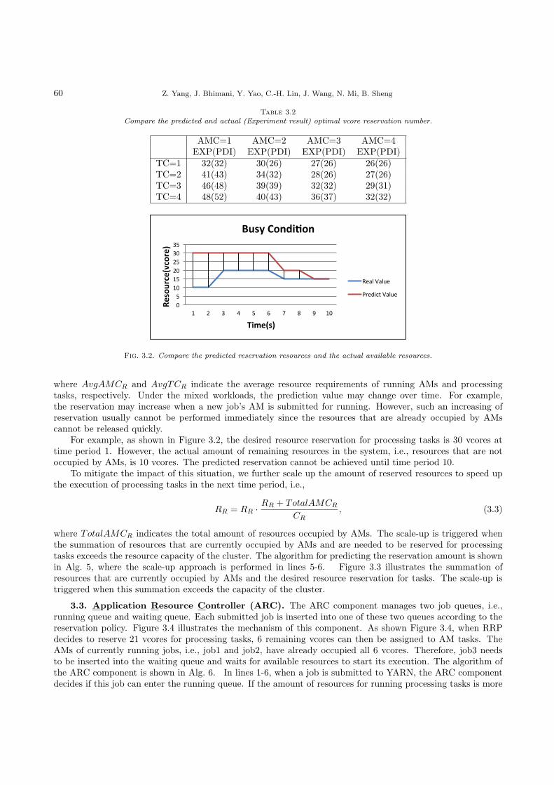
60 Z. Yang, J. Bhimani, Y. Yao, C.-H. Lin, J. Wang, N. Mi, B. Sheng
Table 3.2
Compare the predicted and actual (Experiment result) optimal vcore reservation number.
AMC=1 AMC=2 AMC=3 AMC=4EXP(PDI) EXP(PDI) EXP(PDI) EXP(PDI)
TC=1 32(32) 30(26) 27(26) 26(26)TC=2 41(43) 34(32) 28(26) 27(26)TC=3 46(48) 39(39) 32(32) 29(31)TC=4 48(52) 40(43) 36(37) 32(32)
0
5
10
15
20
25
30
35
1 2 3 4 5 6 7 8 9 10
Resource(vcore)
Time(s)
Busy Condi4on
Real Value
Predict Value
Fig. 3.2. Compare the predicted reservation resources and the actual available resources.
where AvgAMCR and AvgTCR indicate the average resource requirements of running AMs and processingtasks, respectively. Under the mixed workloads, the prediction value may change over time. For example,the reservation may increase when a new job’s AM is submitted for running. However, such an increasing ofreservation usually cannot be performed immediately since the resources that are already occupied by AMscannot be released quickly.
For example, as shown in Figure 3.2, the desired resource reservation for processing tasks is 30 vcores attime period 1. However, the actual amount of remaining resources in the system, i.e., resources that are notoccupied by AMs, is 10 vcores. The predicted reservation cannot be achieved until time period 10.
To mitigate the impact of this situation, we further scale up the amount of reserved resources to speed upthe execution of processing tasks in the next time period, i.e.,
RR = RR ·
RR + TotalAMCR
CR
, (3.3)
where TotalAMCR indicates the total amount of resources occupied by AMs. The scale-up is triggered whenthe summation of resources that are currently occupied by AMs and are needed to be reserved for processingtasks exceeds the resource capacity of the cluster. The algorithm for predicting the reservation amount is shownin Alg. 5, where the scale-up approach is performed in lines 5-6. Figure 3.3 illustrates the summation ofresources that are currently occupied by AMs and the desired resource reservation for tasks. The scale-up istriggered when this summation exceeds the capacity of the cluster.
3.3. Application Resource Controller (ARC). The ARC component manages two job queues, i.e.,running queue and waiting queue. Each submitted job is inserted into one of these two queues according to thereservation policy. Figure 3.4 illustrates the mechanism of this component. As shown Figure 3.4, when RRPdecides to reserve 21 vcores for processing tasks, 6 remaining vcores can then be assigned to AM tasks. TheAMs of currently running jobs, i.e., job1 and job2, have already occupied all 6 vcores. Therefore, job3 needsto be inserted into the waiting queue and waits for available resources to start its execution. The algorithm ofthe ARC component is shown in Alg. 6. In lines 1-6, when a job is submitted to YARN, the ARC componentdecides if this job can enter the running queue. If the amount of resources for running processing tasks is more
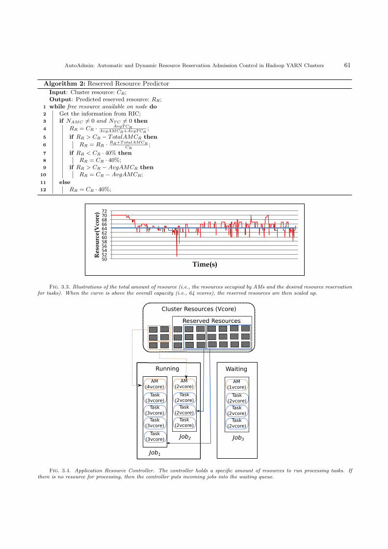
AutoAdmin: Automatic and Dynamic Resource Reservation Admission Control in Hadoop YARN Clusters 61
Algorithm 2: Reserved Resource Predictor
Input: Cluster resource: CR;
Output: Predicted reserved resource: RR;
1 while free resource available on node do
2 Get the information from RIC;
3 if NAMC = 0 and NTC = 0 then
4 RR = CR · AvgTCR
AvgAMCR+AvgTCR
;
5 if RR > CR − TotalAMCR then
6 RR = RR · RR+TotalAMCR
CR;
7 if RR < CR · 40% then
8 RR = CR · 40%;
9 if RR > CR −AvgAMCR then
10 RR = CR −AvgAMCR;
11 else
12 RR = CR · 40%;
50
52
54
56
58
60
62
64
66
68
70
72
Resource(Vcore)
Time(s)
Fig. 3.3. Illustrations of the total amount of resource (i.e., the resources occupied by AMs and the desired resource reservationfor tasks). When the curve is above the overall capacity (i.e., 64 vcores), the reserved resources are then scaled up.
Cluster Resources (Vcore)
AM
(2vcore)
Task
(2vcore)
Task
(2vcore)
Task
(2vcore)
AM
(4vcore)
Task
(3vcore)
Task
(3vcore)
Task
(3vcore)
Task
(3vcore)
Job1
Job2
AM
(1vcore)
Task
(2vcore)
Task
(2vcore)
Task
(2vcore)
Job3
Running Waiting
Fig. 3.4. Application Resource Controller. The controller holds a specific amount of resources to run processing tasks. Ifthere is no resource for processing, then the controller puts incoming jobs into the waiting queue.
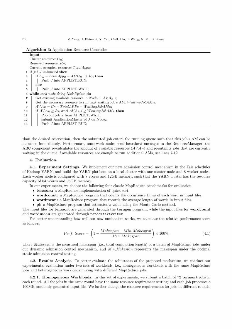
62 Z. Yang, J. Bhimani, Y. Yao, C.-H. Lin, J. Wang, N. Mi, B. Sheng
Algorithm 3: Application Resource Controller
Input:
Cluster resource: CR;
Reserved resource: RR;
Current occupied resource: TotalAppR;
1 if job J submitted then
2 if CR − TotalAppR −AMCRJ≥ RR then
3 Push J into APPLIST RUN;
4 else
5 Push J into APPLIST WAIT;
6 while each node doing NodeUpdate do
7 Get existing available resource in Nodei : AV AR i;
8 Get the necessary resource to run next waiting job’s AM: WaitingJobAMR;
9 AV AR = CR − TotalAPPR −WaitingJobAMR;
10 if AV AR ≥ RR and AV AR i ≥ WaitingJobAMR then
11 Pop out job J from APPLIST WAIT;
12 submit ApplicationMaster of J on Nodei;
13 Push J into APPLIST RUN;
than the desired reservation, then the submitted job enters the running queue such that this job’s AM can belaunched immediately. Furthermore, once work nodes send heartbeat messages to the ResourceManager, theARC component re-calculates the amount of available resources (AV AR) and re-submits jobs that are currentlywaiting in the queue if available resources are enough to run additional AMs, see lines 7-12.
4. Evaluation.
4.1. Experiment Settings. We implement our new admission control mechanism in the Fair schedulerof Hadoop YARN, and build the YARN platform on a local cluster with one master node and 8 worker nodes.Each worker node is configured with 8 vcores and 12GB memory, such that the YARN cluster has the resourcecapacity of 64 vcores and 96GB memory.
In our experiments, we choose the following four classic MapReduce benchmarks for evaluation.• terasort: a MapReduce implementation of quick sort.• wordcount: a MapReduce program that counts the occurrence times of each word in input files.• wordmean: a MapReduce program that records the average length of words in input files.• pi: a MapReduce program that estimates π value using the Monte Carlo method.
The input files for terasort are generated through the teragen program, while the input files for wordcountand wordmean are generated through randomtextwriter.
For better understanding how well our new mechanism works, we calculate the relative performance scoreas follows:
Perf. Score =
(
1−Makespan−Min Makespan
Min Makespan
)
× 100%, (4.1)
where Makespan is the measured makespan (i.e., total completion length) of a batch of MapReduce jobs underour dynamic admission control mechanism, and Min Makespan represents the makespan under the optimalstatic admission control setting.
4.2. Results Analysis. To better evaluate the robustness of the proposed mechanism, we conduct ourexperimental evaluation under two sets of workloads, i.e., homogeneous workloads with the same MapReducejobs and heterogeneous workloads mixing with different MapReduce jobs.
4.2.1. Homogeneous Workloads. In this set of experiments, we submit a batch of 72 terasort jobs ineach round. All the jobs in the same round have the same resource requirement setting, and each job processes a100MB randomly generated input file. We further change the resource requirements for jobs in different rounds,

AutoAdmin: Automatic and Dynamic Resource Reservation Admission Control in Hadoop YARN Clusters 63
Table 4.1
Perf. Scores under homogeneous workloads.
AMC=1 AMC=2 AMC=3 AMC=4TC=1 90.4% 99.6% 89.3% 91.4%TC=2 99.3% 95.6% 99.4% 91.7%TC=3 97.6% 99.2% 96.9% 97.4%TC=4 88.5% 90.5% 99.7% 98.5%
i.e., from 1 vcore to 4 vcores for both ApplicationMasters and processing tasks. Therefore, there are totally16 rounds with different resource requirement combinations. The performance (e.g., makespans) under ouradmission control mechanism which dynamically sets the resource reservations (see red lines) as well as differentstatic reservation configurations (see blue lines) is depicted in Figure 4.1. The corresponding Perf. Scores ofour new mechanism are also shown in Table 4.1.
We first observe that different resource requirements need different amounts of reserved resources (e.g.,numbers of vcores) for running tasks in order to achieve the best performance, i.e., the minimum makespan, seeblue curves in Figure 4.1. However, it is inherently difficult to statically find such an optimal reservation level,especially if resource requirements are not fixed. While, by dynamically tuning the resource reservation level,our admission control mechanism always obtains the best performance compared to the results under the staticresource reservations under almost all resource requirement configurations, see red lines in the figure. Table 4.1further demonstrates that our new mechanism achieves high Perf. Scores, e.g., under more than half of thecases, Perf. Scores are greater than 95%.
4.2.2. Heterogeneous. Now, we turn to evaluate our new mechanism under a more challenging scenario,where we consider heterogeneous workloads which are mixed with different MapReduce jobs. Specifically, wechoose more than two MapReduce benchmarks and submit a batch of jobs from these benchmarks which areconfigured with different resource requirements for running their ApplicationMasters and tasks. We totallyconduct 6 sets of experiments with different combinations of MapReduce jobs. Table 4.2 shows the detailedconfigurations for each set of experiments.
The experimental results (e.g., the makespans and the Perf. Scores) under heterogeneous workloads areshown in Figure 4.2 and Table 4.3, respectively. Consistent with the case of homogeneous workloads, wecan see that our proposed mechanism can still work well under various heterogeneous MapReduce workloads,which achieves the performance close to those under optimal static resource reservations. On the other hand,the settings for optimal static resource reservations are varying across different heterogeneous workloads. Aninappropriate configuration could dramatically degrade the performance. Therefore, our mechanism whichdynamically and automatically controls the admission of applications (i.e., reserving resources for runningregular tasks) is important for achieving competitive performance of YARN.
5. Related Works. While the original Hadoop MapReduce framework has been extensively studied inrecent years, Hadoop YARN is relatively new and has not been widely studied yet. A few preliminary workshave been presented to improve the scheduling in Hadoop YARN systems. Dominant resource fairness [14] wasproposed to improve the fairness between users when multiple types of resources are required by MapReducejobs as in YARN framework. Some previous studies [13] [6] designed modified frameworks to handle iterativejobs. These works attempt to achieve performance improvements on share-based scheduling in Hadoop YARN.However, the deadlock problem caused by ApplicationMasters has not been considered yet.
Simple admission control policy that could help avoid deadlocks is supported in Fair [3] and Capacity [2]schedulers of YARN. For example, users can specify the maximum number of jobs for each queue under theFair scheduler. By manually specifying a small number of jobs that are allowed in each queue concurrently, theApplicationMasters of these jobs will not occupy all system resources. However, it is difficult for administratorsto manually choose a good configuration. Moreover, static configurations cannot work well, especially underdynamic workloads.
Admission control in cloud computing has also been well studied in different aspects. Wu et al. [23]proposed admission control policies that aimed to maximize the SaaS provider’s profits based on user SLA

64 Z. Yang, J. Bhimani, Y. Yao, C.-H. Lin, J. Wang, N. Mi, B. Sheng
0
20
0
40
0
60
0
80
0
10
00 2
0 2
5 3
0 3
5 4
0 4
5 5
0 5
5
Makespan(sec)
Static reserv
ed v
cores
AM
(1co
re)−T
ask(2
cores)
0
20
0
40
0
60
0
80
0
10
00 2
0 2
5 3
0 3
5 4
0 4
5 5
0 5
5
Makespan(sec)
Static reserv
ed v
cores
AM
(1co
re)−T
ask(3
cores)
0
20
0
40
0
60
0
80
0
10
00 2
0 2
5 3
0 3
5 4
0 4
5 5
0 5
5
Makespan(sec)
Static reserv
ed v
cores
AM
(1co
re)−T
ask(4
cores)
0
20
0
40
0
60
0
80
0
10
00
12
00 2
0 2
5 3
0 3
5 4
0 4
5 5
0 5
5
Makespan(sec)
Static reserv
ed v
cores
AM
(2co
res)−T
ask(4
cores)
0
20
0
40
0
60
0
80
0
10
00
12
00 2
0 2
5 3
0 3
5 4
0 4
5 5
0 5
5
Makespan(sec)
Static reserv
ed v
cores
AM
(2co
res)−T
ask(3
cores)
0
20
0
40
0
60
0
80
0
10
00
12
00 2
0 2
5 3
0 3
5 4
0 4
5 5
0 5
5
Makespan(sec)S
tatic reserved
vco
res
AM
(2co
res)−T
ask(2
cores)
0
20
0
40
0
60
0
80
0
10
00
12
00 2
0 2
5 3
0 3
5 4
0 4
5 5
0 5
5
Makespan(sec)
Static reserv
ed v
cores
AM
(2co
res)−T
ask(1
core)
0 2
00
40
0 6
00
80
0 1
00
0 1
20
0 1
40
0 1
60
0 1
80
0 20
25
30
35
40
45
50
55
Makespan(sec)
Static reserv
ed v
cores
AM
(3co
res)−T
ask(1
core)
0 2
00
40
0 6
00
80
0 1
00
0 1
20
0 1
40
0 1
60
0 1
80
0 20
25
30
35
40
45
50
55
Makespan(sec)
Static reserv
ed v
cores
AM
(3co
res)−T
ask(2
cores)
0 2
00
40
0 6
00
80
0 1
00
0 1
20
0 1
40
0 1
60
0 1
80
0 20
25
30
35
40
45
50
55
Makespan(sec)
Static reserv
ed v
cores
AM
(3co
res)−T
ask(3
cores)
0 2
00
40
0 6
00
80
0 1
00
0 1
20
0 1
40
0 1
60
0 1
80
0 20
25
30
35
40
45
50
55
Makespan(sec)
Static reserv
ed v
cores
AM
(3co
res)−T
ask(4
cores)
0
50
0
10
00
15
00
20
00 2
0 2
5 3
0 3
5 4
0 4
5 5
0 5
5
Makespan(sec)
Static reserv
ed v
cores
AM
(4co
res)−T
ask(4
cores)
0
50
0
10
00
15
00
20
00 2
0 2
5 3
0 3
5 4
0 4
5 5
0 5
5
Makespan(sec)
Static reserv
ed v
cores
AM
(4co
res)−T
ask(3
cores)
0
50
0
10
00
15
00
20
00 2
0 2
5 3
0 3
5 4
0 4
5 5
0 5
5
Makespan(sec)
Static reserv
ed v
cores
AM
(4co
res)−T
ask(2
cores)
0
50
0
10
00
15
00
20
00 2
0 2
5 3
0 3
5 4
0 4
5 5
0 5
5
Makespan(sec)
Static reserv
ed v
cores
AM
(4co
res)−T
ask(1
core)
0
20
0
40
0
60
0
80
0
10
00 2
0 2
5 3
0 3
5 4
0 4
5 5
0 5
5
Makespan(sec)
Static reserv
ed v
cores
AM
(1co
re)−T
ask(1
core)
Fig.4.1.Makespa
nsunder
homogen
eousworkloa
ds,
where
thesolid
curves
show
theresu
ltsunder
differen
tsta
ticreserva
tionconfigu
ratio
nsandthered
dashed-lin
espresen
ttheresu
ltsunder
ourmech
anism
which
dynamica
llysets
thereso
urce
reservatio
ns.
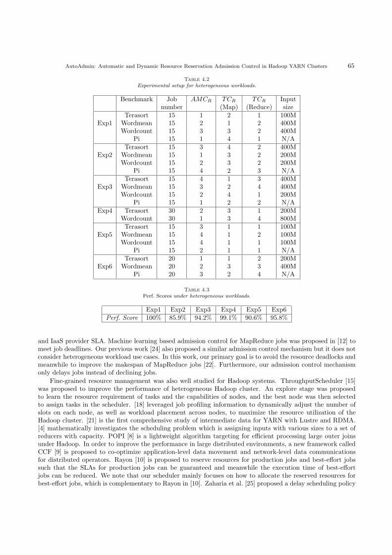
AutoAdmin: Automatic and Dynamic Resource Reservation Admission Control in Hadoop YARN Clusters 65
Table 4.2
Experimental setup for heterogeneous workloads.
Benchmark Job AMCR TCR TCR Inputnumber (Map) (Reduce) size
Terasort 15 1 2 1 100MExp1 Wordmean 15 2 1 2 400M
Wordcount 15 3 3 2 400MPi 15 1 4 1 N/A
Terasort 15 3 4 2 400MExp2 Wordmean 15 1 3 2 200M
Wordcount 15 2 3 2 200MPi 15 4 2 3 N/A
Terasort 15 4 1 3 400MExp3 Wordmean 15 3 2 4 400M
Wordcount 15 2 4 1 200MPi 15 1 2 2 N/A
Exp4 Terasort 30 2 3 1 200MWordcount 30 1 3 4 800MTerasort 15 3 1 1 100M
Exp5 Wordmean 15 4 1 2 100MWordcount 15 4 1 1 100M
Pi 15 2 1 1 N/ATerasort 20 1 1 2 200M
Exp6 Wordmean 20 2 3 3 400MPi 20 3 2 4 N/A
Table 4.3
Perf. Scores under heterogeneous workloads.
Exp1 Exp2 Exp3 Exp4 Exp5 Exp6Perf. Score 100% 85.9% 94.2% 99.1% 90.6% 95.8%
and IaaS provider SLA. Machine learning based admission control for MapReduce jobs was proposed in [12] tomeet job deadlines. Our previous work [24] also proposed a similar admission control mechanism but it does notconsider heterogeneous workload use cases. In this work, our primary goal is to avoid the resource deadlocks andmeanwhile to improve the makespan of MapReduce jobs [22]. Furthermore, our admission control mechanismonly delays jobs instead of declining jobs.
Fine-grained resource management was also well studied for Hadoop systems. ThroughputScheduler [15]was proposed to improve the performance of heterogeneous Hadoop cluster. An explore stage was proposedto learn the resource requirement of tasks and the capabilities of nodes, and the best node was then selectedto assign tasks in the scheduler. [18] leveraged job profiling information to dynamically adjust the number ofslots on each node, as well as workload placement across nodes, to maximize the resource utilization of theHadoop cluster. [21] is the first comprehensive study of intermediate data for YARN with Lustre and RDMA.[4] mathematically investigates the scheduling problem which is assigning inputs with various sizes to a set ofreducers with capacity. POPI [8] is a lightweight algorithm targeting for efficient processing large outer joinsunder Hadoop. In order to improve the performance in large distributed environments, a new framework calledCCF [9] is proposed to co-optimize application-level data movement and network-level data communicationsfor distributed operators. Rayon [10] is proposed to reserve resources for production jobs and best-effort jobssuch that the SLAs for production jobs can be guaranteed and meanwhile the execution time of best-effortjobs can be reduced. We note that our scheduler mainly focuses on how to allocate the reserved resources forbest-effort jobs, which is complementary to Rayon in [10]. Zaharia et al. [25] proposed a delay scheduling policy
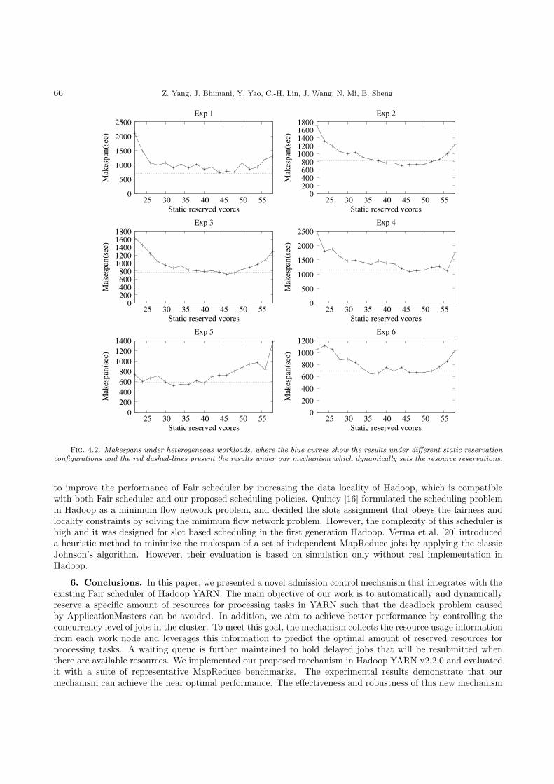
66 Z. Yang, J. Bhimani, Y. Yao, C.-H. Lin, J. Wang, N. Mi, B. Sheng
0 200 400 600 800
1000 1200 1400 1600 1800
25 30 35 40 45 50 55
Mak
espan
(sec
)
Static reserved vcores
Exp 2
0
500
1000
1500
2000
2500
25 30 35 40 45 50 55
Mak
espan
(sec
)
Static reserved vcores
Exp 4
0 200 400 600 800
1000 1200 1400 1600 1800
25 30 35 40 45 50 55
Mak
espan
(sec
)
Static reserved vcores
Exp 3
0
200
400
600
800
1000
1200
1400
25 30 35 40 45 50 55
Mak
espan
(sec
)
Static reserved vcores
Exp 5
0
200
400
600
800
1000
1200
25 30 35 40 45 50 55
Mak
espan
(sec
)
Static reserved vcores
Exp 6
0
500
1000
1500
2000
2500
25 30 35 40 45 50 55
Mak
espan
(sec
)
Static reserved vcores
Exp 1
Fig. 4.2. Makespans under heterogeneous workloads, where the blue curves show the results under different static reservationconfigurations and the red dashed-lines present the results under our mechanism which dynamically sets the resource reservations.
to improve the performance of Fair scheduler by increasing the data locality of Hadoop, which is compatiblewith both Fair scheduler and our proposed scheduling policies. Quincy [16] formulated the scheduling problemin Hadoop as a minimum flow network problem, and decided the slots assignment that obeys the fairness andlocality constraints by solving the minimum flow network problem. However, the complexity of this scheduler ishigh and it was designed for slot based scheduling in the first generation Hadoop. Verma et al. [20] introduceda heuristic method to minimize the makespan of a set of independent MapReduce jobs by applying the classicJohnson’s algorithm. However, their evaluation is based on simulation only without real implementation inHadoop.
6. Conclusions. In this paper, we presented a novel admission control mechanism that integrates with theexisting Fair scheduler of Hadoop YARN. The main objective of our work is to automatically and dynamicallyreserve a specific amount of resources for processing tasks in YARN such that the deadlock problem causedby ApplicationMasters can be avoided. In addition, we aim to achieve better performance by controlling theconcurrency level of jobs in the cluster. To meet this goal, the mechanism collects the resource usage informationfrom each work node and leverages this information to predict the optimal amount of reserved resources forprocessing tasks. A waiting queue is further maintained to hold delayed jobs that will be resubmitted whenthere are available resources. We implemented our proposed mechanism in Hadoop YARN v2.2.0 and evaluatedit with a suite of representative MapReduce benchmarks. The experimental results demonstrate that ourmechanism can achieve the near optimal performance. The effectiveness and robustness of this new mechanism

AutoAdmin: Automatic and Dynamic Resource Reservation Admission Control in Hadoop YARN Clusters 67
are validated under both homogeneous and heterogeneous workloads. In the future, we will investigate therelationship between job concurrency and system throughput in a YARN cluster and further extend our workto other cloud computing platforms.
REFERENCES
[1] Apache hadoop users.[2] Hadoop mapreduce next generation - capacity scheduler.[3] Hadoop mapreduce next generation - fair scheduler.[4] F. Afrati, S. Dolev, E. Korach, S. Sharma, and J. D. Ullman, Assignment problems of different-sized inputs in mapre-
duce, ACM Transactions on Knowledge Discovery from Data (TKDD), 11 (2016), p. 18.[5] Apache, Apache hadoop nextgen mapreduce (yarn).[6] Y. Bu, B. Howe, M. Balazinska, and M. D. Ernst, Haloop: efficient iterative data processing on large clusters, Proceedings
of the VLDB Endowment, 3 (2010), pp. 285–296.[7] Y. Chen, A. Ganapathi, R. Griffith, and R. Katz, The case for evaluating mapreduce performance using workload
suites, in Modeling, Analysis & Simulation of Computer and Telecommunication Systems (MASCOTS), 2011 IEEE 19thInternational Symposium on, IEEE, 2011, pp. 390–399.
[8] L. Cheng and S. Kotoulas, Efficient large outer joins over mapreduce, in European Conference on Parallel Processing,Springer, 2016, pp. 334–346.
[9] L. Cheng, Y. Wang, Y. Pei, and D. Epema, A coflow-based co-optimization framework for high-performance data analytics,in Parallel Processing (ICPP), 2017 46th International Conference on, IEEE, 2017, pp. 392–401.
[10] C. Curino, D. E. Difallah, C. Douglas, S. Krishnan, R. Ramakrishnan, and S. Rao, Reservation-based scheduling: Ifyou’re late don’t blame us!, in Proceedings of the ACM Symposium on Cloud Computing, ACM, 2014, pp. 1–14.
[11] J. Dean and S. Ghemawat, Mapreduce: simplified data processing on large clusters, Communications of the ACM, 51 (2008),pp. 107–113.
[12] J. Dhok, N. Maheshwari, and V. Varma, Learning based opportunistic admission control algorithm for mapreduce as aservice, in Proceedings of the 3rd India software engineering conference, ACM, 2010, pp. 153–160.
[13] J. Ekanayake, H. Li, B. Zhang, T. Gunarathne, S.-H. Bae, J. Qiu, and G. Fox, Twister: a runtime for iterativemapreduce, in Proceedings of the 19th ACM International Symposium on High Performance Distributed Computing,ACM, 2010, pp. 810–818.
[14] A. Ghodsi, M. Zaharia, B. Hindman, A. Konwinski, S. Shenker, and I. Stoica, Dominant resource fairness: Fairallocation of multiple resource types., in NSDI, vol. 11, 2011, pp. 24–24.
[15] S. Gupta, C. Fritz, B. Price, R. Hoover, J. de Kleer, and C. Witteveen, Throughputscheduler: Learning to schedule onheterogeneous hadoop clusters, in Proceedings 10th ACM International Conference on Autonomic Computing (ICAC’13),ACM.
[16] M. Isard, V. Prabhakaran, J. Currey, U. Wieder, K. Talwar, and A. Goldberg, Quincy: fair scheduling for distributedcomputing clusters, in Proceedings of the ACM SIGOPS 22nd symposium on Operating systems principles, ACM, 2009,pp. 261–276.
[17] A. Murthy, Apache hadoop yarn - concepts and applications.[18] J. Polo, C. Castillo, D. Carrera, Y. Becerra, I. Whalley, M. Steinder, J. Torres, and E. Ayguade, Resource-aware
adaptive scheduling for mapreduce clusters, in Middleware 2011, Springer, 2011, pp. 187–207.[19] V. K. Vavilapalli, A. C. Murthy, C. Douglas, et al., Apache hadoop yarn: Yet another resource negotiator, in Proceedings
of the 4th annual Symposium on Cloud Computing, ACM, 2013.[20] A. Verma, L. Cherkasova, and R. H. Campbell, Two sides of a coin: Optimizing the schedule of mapreduce jobs to min-
imize their makespan and improve cluster performance, in Modeling, Analysis & Simulation of Computer and Telecom-munication Systems (MASCOTS), 2012 IEEE 20th International Symposium on, IEEE, 2012, pp. 11–18.
[21] M. Wasi-ur Rahman, N. S. Islam, X. Lu, and D. K. D. Panda, A comprehensive study of mapreduce over lustre for inter-mediate data placement and shuffle strategies on hpc clusters, IEEE Transactions on Parallel and Distributed Systems,28 (2017), pp. 633–646.
[22] M. Wojnowicz, D. Nguyen, L. Li, and X. Zhao, Lazy stochastic principal component analysis, in IEEE InternationalConference on Data Mining Workshop, 2017.
[23] L. Wu, S. Kumar Garg, and R. Buyya, Sla-based admission control for a software-as-a-service provider in cloud computingenvironments, Journal of Computer and System Sciences, 78 (2012), pp. 1280–1299.
[24] Y. Yao, J. Lin, J. Wang, N. Mi, and B. Sheng, Admission control in yarn clusters based on dynamic resource reservation,in Integrated Network Management (IM), 2015 IFIP/IEEE International Symposium on, IEEE, 2015, pp. 838–841.
[25] M. Zaharia, D. Borthakur, J. Sen Sarma, K. Elmeleegy, S. Shenker, and I. Stoica, Delay scheduling: a simpletechnique for achieving locality and fairness in cluster scheduling, in Proceedings of the 5th European conference onComputer systems, ACM, 2010, pp. 265–278.
Edited by: Pradeep Reddy CHReceived: Jun 7, 2017Accepted: Feb 26, 2018


Scalable Computing: Practice and Experience
Volume 19, Number 1, pp. 69–77. http://www.scpe.org
DOI 10.12694/scpe.v19i1.1394ISSN 1895-1767c⃝ 2018 SCPE
AN OPTIMIZED DENSITY-BASED ALGORITHM FOR ANOMALY DETECTION IN
HIGH DIMENSIONAL DATASETS
ADEEL SHIRAZ HASHMI∗, MOHAMMAD NAJMUD DOJA †, AND TANVIR AHMAD ‡
Abstract. In this study, the authors aim to propose an optimized density-based algorithm for anomaly detection with focuson high-dimensional datasets. The optimization is achieved by optimizing the input parameters of the algorithm using fireflymeta-heuristic. The performance of different similarity measures for the algorithm is compared including both L1 and L2 norms toidentify the most efficient similarity measure for high-dimensional datasets. The algorithm is optimized further in terms of speedand scalability by using Apache Spark big data platform. The experiments were conducted on publicly available datasets, and theresults were evaluated on various performance metrics like execution time, accuracy, sensitivity, and specificity.
Key words: Anomaly detection, outlier detection, optimization, similarity measures, data mining
AMS subject classifications. 68P05, 68W15, 68W25
1. Introduction. In this era of big data, the traditional data mining algorithms are not capable of handlinghigh-dimensional, high-volume datasets efficiently. To handle such datasets, new algorithms need to be proposedor the existing algorithms should be modified. Anomaly/Outlier detection [6][4][1] is a significant field of researchin data mining and like other data mining algorithms, anomaly detection algorithms also need to be enhancedto handle such datasets. The algorithm should not only be accurate, but it should also be scalable and fastenough to identify the anomaly in real-time from the vast amount of data that is being generated every second.
This paper discusses how an anomaly detection algorithm can be optimized to make it faster and moreaccurate, with focus on handling high dimensional datasets. Most of these algorithms provide the resultsbased on some input parameters, and optimization of these parameters is must to obtain high accuracy for thealgorithm. These algorithms also make use of some distance/similarity measure to identify the outliers andselection of this distance measure significantly affects the accuracy as well as speed of the algorithm. Furtherto increase the speed of the algorithm, it can be parallelized to reduce the processing time considerably. So,optimization of the parameters, selection of distance measure, and parallel implementation can collectivelyhave a huge impact on accuracy and speed of the algorithm. This paper aims to propose an efficient anomalydetection algorithm for high-dimensional datasets based on all these fore-mentioned observations.
Local Correlation Integral [13] is a popular anomaly detection algorithm based on identifying the neigh-borhoods of every instance in the dataset by using a distance/ similarity measure like Euclidean distance, andthe instances which are identified as isolated are deemed to be the outliers. In this paper, the authors aim tooptimize a LOCI-inspired algorithm for anomaly detection; one of the objectives is to optimize the input param-eters, and the only input parameter for this algorithm is the radius of the neighborhood. To optimize this radiusthreshold, the authors select a swarm intelligence meta-heuristic, which is the firefly algorithm. The secondphase of optimization deals with the similarity measure used by the algorithm, where the authors aim to findwhich similarity measure is optimal while dealing with high dimensional datasets. So, both L1 and L2 normswere compared for accuracy as well as speed. The platform chosen for conducting the experiments is ApacheSpark as it guarantees scalability, fault-tolerance and also provides quick results by distributed processing andin-memory analytical abilities.
2. Related Work. In this section, we will review the literature dealing with anomaly detection followedby optimization algorithms which can be utilized to optimize the input parameters.
2.1. Anomaly detection. Anomaly Detection is a field of data mining dealing with finding abnormaldata points in the given dataset. The major application areas of anomaly detection are intrusion-detectionin the field of network security, fraud detection in financial domain, finding misbehaving node in the wireless
∗ Department of Computer Engineering, Faculty of Engineering and Technology, Jamia Millia Islamia, New Delhi, India([email protected]).
†Department of Computer Engineering, Faculty of Engineering and Technology, Jamia Millia Islamia, New Delhi, India.‡ Department of Computer Engineering, Faculty of Engineering and Technology, Jamia Millia Islamia, New Delhi, India
69

70 A. Shiraz Hashmi, M. Najmud Doja, T. Ahmad
sensor networks, medical and healthcare datasets, etc. With the rise of big data, finding anomalies in largedatasets in real-time is quite a challenging task. So, we need to develop new faster algorithms or to optimizeexisting algorithms so that outliers are detected before it is too late in critical real-time environments.
The simplest and fastest anomaly detection algorithm is the AVF (Attribute Value Frequency) [8] which isbased on the assumption that the data points with low frequencies are the prime candidates to be the outliers.Another statistical algorithm is the Entropy-based Outlier Detection (EBOD) [9] which assumes that the pointswhose removal causes the maximum decrease in the entropy of the dataset are the anomalies. There are graphicaltechniques for outlier detection as well, namely, scatter-plots and box-plots; however these graphical techniquesfail for multi-dimensional datasets.
Machine Learning based algorithms are also available for anomaly detection. DBSCAN [7] is a clusteringalgorithm with ability to identify anomalies, whereas OPTICS-OF [2] is an extension of OPTICS clusteringalgorithm for anomaly detection. Neural Networks have been utilized in literature in the form of ReplicatorNeural Networks for finding outliers. LOF (Local Outlier Factor) [3] and LOCI (Local Correlation Integral) [13]are the two most popular algorithms for anomaly detection, provided by most of the machine learning libraries.
2.2. Optimization Algorithms. In artificial intelligence, a metaheuristic is a partial search algorithmwhich finds a sufficiently good solution when there is no proper information for guiding the search process,and going through all the possible states is not feasible. Metaphor-based metaheuristics are nature-inspiredmetaheuristics like simulated annealing which is based on a naturally occurring chemical process. Evolutionaryalgorithms [12] are a category of population-based metaheuristics which start with random solutions and movetowards an optimal solution. A category of evolutionary algorithms is swarm-based algorithms which mimic thecollective behavior of insects/organisms/animals shown while searching for food, finding mating partner, etc.There are many swarm-based metaheuristics mostly derived from the PSO (Particle Swarm Optimization) andACO (Ant Colony Optimization) metaheuristics like Firefly Algorithm, Bat Algorithm, Cuckoo Search, FishSchool Search, etc. Some of the popular swarm-based metaheuristics are listed in Table 2.1.
The swarm intelligence optimization is based on two processes: exploitation and exploration. The exploita-tion process deals with finding the best solution among the present candidate solutions (local best), whereasexploration process deals with generating new candidate solutions to reach a global best. The exploration isachieved by a random walk in the search space. Levy flight [14][17] is a random walk which is used by most ofthe researchers for exploration in the swarm-based optimization algorithms.
Table 2.1
Swarm-based Metaheuristics
Algorithm Year Proposed byAnt Colony Optimization 1992 Dorigo, Di CaroParticle Swarm Optimization 1995 Kennedy, Eberhart, ShiHarmony Search 2001 Geem, Kim, LoganathanBacterial Foraging Algorithm 2002 PassinoArtificial Bee Colony 2007 Karaboga, BasturkFirefly Algorithm 2008 Xin She-YangCuckoo Search 2009 Xin She-Yang, DebBat Algorithm 2010 Xin She-YangFlower Pollination 2012 Xin She-YangCuttlefish Optimization Algorithm 2013 Eesa et al.Artificial Swarm Intelligence 2014 Louis ResenbergGrey Wolf Optimizer 2014 Seyedali MirjaliliAnt Lion Optimizer 2015 Seyedali MirjaliliMoth Flame Optimization 2015 Seyedali MirjaliliDragonfly Algorithm 2015 Seyedali MirjaliliWhale Optimizer 2016 Seyedali Mirjalili
Most of the swarm-based optimization algorithms are based on the particle swarm optimization algorithm.
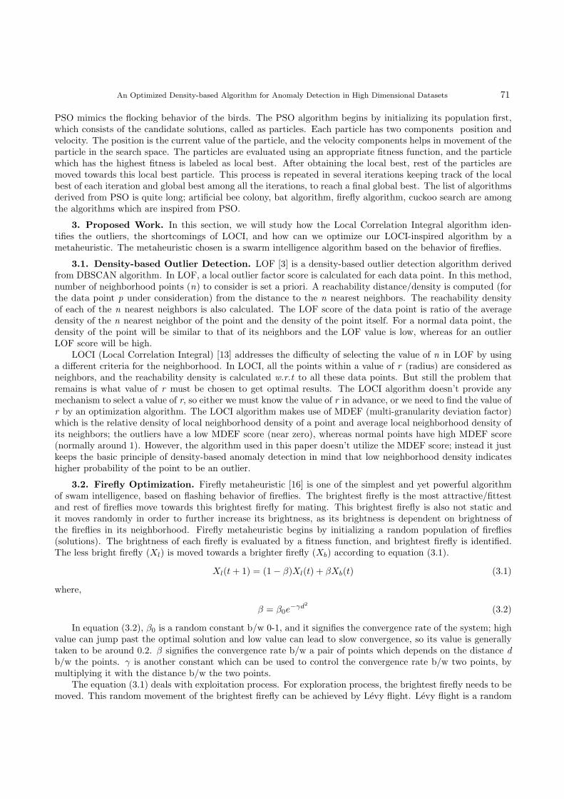
An Optimized Density-based Algorithm for Anomaly Detection in High Dimensional Datasets 71
PSO mimics the flocking behavior of the birds. The PSO algorithm begins by initializing its population first,which consists of the candidate solutions, called as particles. Each particle has two components position andvelocity. The position is the current value of the particle, and the velocity components helps in movement of theparticle in the search space. The particles are evaluated using an appropriate fitness function, and the particlewhich has the highest fitness is labeled as local best. After obtaining the local best, rest of the particles aremoved towards this local best particle. This process is repeated in several iterations keeping track of the localbest of each iteration and global best among all the iterations, to reach a final global best. The list of algorithmsderived from PSO is quite long; artificial bee colony, bat algorithm, firefly algorithm, cuckoo search are amongthe algorithms which are inspired from PSO.
3. Proposed Work. In this section, we will study how the Local Correlation Integral algorithm iden-tifies the outliers, the shortcomings of LOCI, and how can we optimize our LOCI-inspired algorithm by ametaheuristic. The metaheuristic chosen is a swarm intelligence algorithm based on the behavior of fireflies.
3.1. Density-based Outlier Detection. LOF [3] is a density-based outlier detection algorithm derivedfrom DBSCAN algorithm. In LOF, a local outlier factor score is calculated for each data point. In this method,number of neighborhood points (n) to consider is set a priori. A reachability distance/density is computed (forthe data point p under consideration) from the distance to the n nearest neighbors. The reachability densityof each of the n nearest neighbors is also calculated. The LOF score of the data point is ratio of the averagedensity of the n nearest neighbor of the point and the density of the point itself. For a normal data point, thedensity of the point will be similar to that of its neighbors and the LOF value is low, whereas for an outlierLOF score will be high.
LOCI (Local Correlation Integral) [13] addresses the difficulty of selecting the value of n in LOF by usinga different criteria for the neighborhood. In LOCI, all the points within a value of r (radius) are considered asneighbors, and the reachability density is calculated w.r.t to all these data points. But still the problem thatremains is what value of r must be chosen to get optimal results. The LOCI algorithm doesn’t provide anymechanism to select a value of r, so either we must know the value of r in advance, or we need to find the value ofr by an optimization algorithm. The LOCI algorithm makes use of MDEF (multi-granularity deviation factor)which is the relative density of local neighborhood density of a point and average local neighborhood density ofits neighbors; the outliers have a low MDEF score (near zero), whereas normal points have high MDEF score(normally around 1). However, the algorithm used in this paper doesn’t utilize the MDEF score; instead it justkeeps the basic principle of density-based anomaly detection in mind that low neighborhood density indicateshigher probability of the point to be an outlier.
3.2. Firefly Optimization. Firefly metaheuristic [16] is one of the simplest and yet powerful algorithmof swam intelligence, based on flashing behavior of fireflies. The brightest firefly is the most attractive/fittestand rest of fireflies move towards this brightest firefly for mating. This brightest firefly is also not static andit moves randomly in order to further increase its brightness, as its brightness is dependent on brightness ofthe fireflies in its neighborhood. Firefly metaheuristic begins by initializing a random population of fireflies(solutions). The brightness of each firefly is evaluated by a fitness function, and brightest firefly is identified.The less bright firefly (Xl) is moved towards a brighter firefly (Xb) according to equation (3.1).
Xl(t+ 1) = (1− β)Xl(t) + βXb(t) (3.1)
where,
β = β0e−γd2
(3.2)
In equation (3.2), β0 is a random constant b/w 0-1, and it signifies the convergence rate of the system; highvalue can jump past the optimal solution and low value can lead to slow convergence, so its value is generallytaken to be around 0.2. β signifies the convergence rate b/w a pair of points which depends on the distance db/w the points. γ is another constant which can be used to control the convergence rate b/w two points, bymultiplying it with the distance b/w the two points.
The equation (3.1) deals with exploitation process. For exploration process, the brightest firefly needs to bemoved. This random movement of the brightest firefly can be achieved by Levy flight. Levy flight is a random

72 A. Shiraz Hashmi, M. Najmud Doja, T. Ahmad
walk in which sudden large steps are taken amidst small steps. The generation of Levy steps can be achievedby Mantegnas algorithm [10], where the step length S can be calculated by equation (3.3):
S =u
v1β
(3.3)
u ≈ N(0, σ2u) and v ≈ N(0, σ2
v) (3.4)
σv = 1 and σu =
Γ(1 + β)sin(
πβ2
)
Γ( 1+β2
)β2(β−1)
2
1β
(3.5)
where β is a parameter b/w interval [1,2] generally taken as 1.5, u and v are drawn from normal distribution,and Γn=(n-1)! is the gamma function.
The firefly metaheuristic can easily be applied for optimizing the value of input parameter r in our anomalydetection algorithm. For optimizing the value of r, the fitness function is k/r and we have to minimize thisfitness function. However, the value of r should not be too high so as to include all the points or too low suchthat every point has small value of k. So, we need to set a lower limit as well as an upper limit on the value ofk. So, according to [11] the fitness function that could be used is:
α
rk+
k
r+
k
n− k(3.6)
Therefore, the fireflies in our case will be the values of r. For each value of r, the fitness of each point iscalculated from equation (3.6).
Steps for anomaly detection by firefly optimized algorithm
Step-1. Initialization.Generate the distance matrix dist mat of the dataset.Define a list with N values of radius r, each value of r corresponding to a firefly.
Step-2. Calculate brightness of each firefly.foreach r in list do
foreach row in dist max doi. find number of elements less than r (set this value as k).ii. find fitness of the row acc. to Eq. 3.6.
Find the row with minimum value of fitness function. The fitness of this row is the brightness of r/firefly.
Step-3. Identify brightest firefly.In previous step, we get N fitness values corresponding to brightness of each firefly.The firefly (value of r) with least fitness value is the brightest firefly, denoted by r*.
Step-4. Move fireflies.foreach r in list do
if(r !=r* )update r acc. to Eq. 3.1.
elseupdate r* by Levy flight.
Step-5. Repeat Steps 3 and 4 for fixed number of iterations.
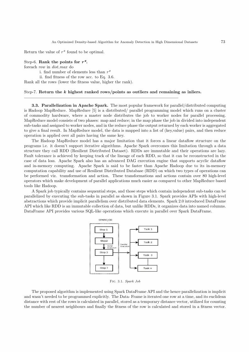
An Optimized Density-based Algorithm for Anomaly Detection in High Dimensional Datasets 73
Return the value of r* found to be optimal.
Step-6. Rank the points for r*.foreach row in dist max do
i. find number of elements less than r*ii. find fitness of the row acc. to Eq. 3.6.
Rank all the rows (lower the fitness value, higher the rank).
Step-7. Return the k highest ranked rows/points as outliers and remaining as inliers.
3.3. Parallelization in Apache Spark. The most popular framework for parallel/distributed computingis Hadoop MapReduce. MapReduce [5] is a distributed/ parallel programming model which runs on a clusterof commodity hardware, where a master node distributes the job to worker nodes for parallel processing.MapReduce model consists of two phases: map and reduce; in the map phase the job in divided into independentsub-tasks and assigned to worker nodes, and in the reduce phase the output returned by each worker is aggregatedto give a final result. In MapReduce model, the data is mapped into a list of (key,value) pairs, and then reduceoperation is applied over all pairs having the same key.
The Hadoop MapReduce model has a major limitation that it forces a linear dataflow structure on theprograms i.e. it doesn’t support iterative algorithms. Apache Spark overcomes this limitation through a datastructure they call RDD (Resilient Distributed Dataset). RDDs are immutable and their operations are lazy.Fault tolerance is achieved by keeping track of the lineage of each RDD, so that it can be reconstructed in thecase of data loss. Apache Spark also has an advanced DAG execution engine that supports acyclic dataflowand in-memory computing. Apache Spark is said to be faster than Apache Hadoop due to its in-memorycomputation capability and use of Resilient Distributed Database (RDD) on which two types of operations canbe performed viz. transformation and action. These transformations and actions contain over 80 high-leveloperators which make development of parallel applications much easier as compared to other MapReduce basedtools like Hadoop.
A Spark job typically contains sequential steps, and those steps which contain independent sub-tasks can beparallelized by executing the sub-tasks in parallel as shown in Figure 3.1. Spark provides APIs with high-levelabstractions which provide implicit parallelism over distributed data elements. Spark 2.0 introduced DataFrameAPI which like RDD is an immutable collection of data, but unlike RDDs, it organizes data into named columns.DataFrame API provides various SQL-like operations which execute in parallel over Spark DataFrame.
Fig. 3.1. Spark Job
The proposed algorithm is implemented using Spark DataFrame API and the hence parallelization is implicitand wasn’t needed to be programmed explicitly. The Data- Frame is iterated one row at a time, and its euclideandistance with rest of the rows is calculated in parallel, stored as a temporary distance vector, utilized for countingthe number of nearest neighbours and finally the fitness of the row is calculated and stored in a fitness vector.

74 A. Shiraz Hashmi, M. Najmud Doja, T. Ahmad
The fitness vector contains fitness value of each row in the dataset. There are N fitness vectors correspondingto N fireflies (values of r). The process of calculating the distance vector is slow when done sequentially, soparallelization of this step improves the performance of the algorithm considerably.
4. Experimental studies. In this section, the experiments conducted on various publicly available data-sets are discussed. The experiments were conducted on i5 processor with 2 cores and 4 GB RAM runningUbuntu 16.10. The algorithm was implemented in PySpark and run over Spark 2.2.0.
4.1. Datasets. The datasets used for experiments are Cardiotocography, Optdigits, Arrhythmia, Musk,Speech and SMTP-KDDCUP99. All these datasets are openly available on UCI/ODDS data repository. TheCardiotocography dataset has 1831 instances with 21 features containing 176 (9.6%) outliers. The Optdigitsdataset has 5216 instances with 64 features containing 150 (3%) outliers. The Arrhythmia dataset has 452instances with 274 features containing 66 (15%) outliers. The Musk dataset has 3062 instances with 166 featurescontaining 97 (3.2%) outliers. Speech dataset has 3686 instances with 400 features containing 61 (1.65%) outliers.SMTP-KDDCUP99 dataset has 95156 instances with 3 features containing 30 (0.03%) outliers.
The Cardiotocography dataset originally has 2126 instances with 23 attributes. The instances are assignedclass normal, suspect or pathologic. The points labeled as suspect are discarded, the normal points are consideredas inliers and the pathologic points are down-sampled to 176.
The Optdigits dataset is a character recognition dataset for integers 0-9. The 32X32 bitmaps are dividedinto non-overlapping blocks of 4X4 each, which generates an input matrix of 8X8. The instances for digits 1-9are treated as inliers whereas the instances of digit 0 are treated as outliers (after down-sampling) to give 150outliers.
Arrhythmia dataset originally has 279 attributes. There are 5 categorical attributes (age, sex, height,weight, class) which are discarded, giving 274 attributes. The 452 instances are assigned to 16 different labelsfrom 01 to 16. The classes with least instances, i.e., 3, 4, 5, 7, 8, 9, 14, 15 are combined to form the outlier class(66 instances) and the rest of the classes are combined to form the inliers class (386 instances).
Musk dataset describes a set of 102 molecules of which 39 are musks and 63 are non-musks. A single moleculecan adopt many shapes due to bond rotations, therefore all the low-energy conformations of the molecules aregenerated to produce 6598 conformations. The naming convention used for the molecules is MOL ISO+CONF.These 6598 conformations are reduced to 3062 conformations, keeping molecules j146, j147 and 252 as non-musk(inliers), whereas molecules 213 and 211 are kept as musks (outliers).
The speech dataset consists of 3686 segments of English speech spoken with eight different accents. Mostof the segments (98.35%) correspond to American accent whereas only 1.65% (61) of the segments belong toone of the seven other accents. So, the segments belonging to American accent are treated as inliers whereassegments belonging to non-American accent are treated as outliers.
The SMTP-KDDCUP99 dataset is a subset of original KDDCUP99 intrusion detection dataset having3925651 attacks (80.1%) out of 4898431 records. A smaller set is forged by having only 3377 attacks (0.35%)of 976157 records, where attribute ’logged in’ is positive. From this forged dataset, 95156 instances of ’SMTP’service data is used to construct the SMTP-KDDCUP99 dataset having 30 (0.03%) outliers.
4.2. Evaluation Metrics. To evaluate and compare our results, we need some evaluation metrics. TP(True positives), FP (False Positives), TN (True Negatives) and FN (False Negatives) are the number of normalpoints correctly detected as inliers, the number of abnormal points that are detected as inliers, the numberof abnormal points that are correctly detected as outliers, and the number of normal points that are wronglydetected as outliers, respectively.
Accuracy, sensitivity, and specificity are defined as the following expressions:
Accuracy =TN + TP
TN + TP + FN + FP(4.1)
Sensitivity =TP
TP + FN(4.2)

An Optimized Density-based Algorithm for Anomaly Detection in High Dimensional Datasets 75
Specificity =TN
TN + FP(4.3)
4.3. Results. In this section, the results of the experiments are discussed. Analyzing the datasets, thesize and feature-to-instance ratio is shown in Table 4.1.
Table 4.1
Analysis of datasets
Dataset Size Values Feature-Instance RatioArrhythmia 452 X 274 123,848 0.6061Cardio 1831 X 21 38,451 0.0114Musk 3062 X 166 508,292 0.0542Speech 3686 X 400 1,474,400 0.1085Optdigits 5216 X 64 333,824 0.0122SMTP KDDCUP99 95156 X 3 285,468 0.00003
From the literature, it is inferred that Euclidean distance is the similarity measure of choice for ordinarydatasets. Table 4.2 provides the execution time to generate the similarity matrices by different similaritymeasures for our chosen datasets. From Table 4.2, we can infer that execution time is primarily dependent onnumber of instances rather than total size of the dataset. Further, it is noticed that Manhattan distance is thebest choice among the chosen distance measures as far as execution time is concerned; the notable exception isthe cardio dataset which has the smallest dimensions among the chosen datasets and for this dataset Euclideandistance has best execution time. It is also noticed that feature-instance ratio has no major impact on choice ofsimilarity measure, as Cardio and Optdigits have nearly same ratio, but results are clearly different. From theseresults we can conclude that Manhattan distance is the best candidate for similarity measure while dealing withhigh-dimensional datasets.
Table 4.2
Execution Time (in seconds) for distance matrix
Data-base
Distance Measures
EuclideanCosineSimilarity
ManhattanDistance
HellingerDistance
Arrythmia 0.145 0.141 0.125 0.134Cardio 1.70 1.66 1.61 1.63Musk 4.75 4.82 4.50 4.67Speech 6.58 6.67 6.42 6.51Optdigits 20.98 14.18 13.74 13.94
Table 4.3 summarizes the accuracy, sensitivity, and specificity of the proposed solution for each dataset. Theresults show that the algorithm returns highly accurate results for all the datasets. Specificity is the indicatorof algorithm’s capability of identifying the outliers, whereas sensitivity and accuracy are the indicators ofalgorithm’s capability of identifying normal instances as well as anomalies.
Table 4.4 compares the performance of proposed firefly-optimized algorithm for anomaly detection withstate-of-the-art algorithms of anomaly detection viz. K-Means, DBSCAN and LOF. The performance compar-ison is done on the basis of accuracy metric using euclidean distance as similarity measure. From the results,it is obvious that the firefly optimized algorithm is far superior in terms of accuracy. The major reason forsuperiority of firefly optimized algorithm is that rest of the algorithms are run with random/default parameterswhereas firefly algorithm is self-optimizing (it optimizes the neighbourhood radius “r”).
5. Conclusion and Future Scope. From the experiments, we can conclude that optimization achievedby firefly algorithm for the value of “r” was quite fruitful as the results were evaluated to be highly accurate.
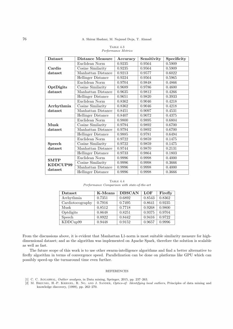
76 A. Shiraz Hashmi, M. Najmud Doja, T. Ahmad
Table 4.3
Performance Metrics
Dataset Distance Measure Accuracy Sensitivity Specificity
Cardiodataset
Euclidean Norm 0.9235 0.9564 0.5909Cosine Similarity 0.9235 0.9564 0.5909Manhattan Distance 0.9213 0.9577 0.6022Hellinger Distance 0.9224 0.9564 0.5965
OptDigitsdataset
Euclidean Norm 0.9704 0.9848 0.4866Cosine Similarity 0.9689 0.9786 0.4600Manhattan Distance 0.9635 0.9812 0.4266Hellinger Distance 0.9651 0.9820 0.3933
Arrhythmiadataset
Euclidean Norm 0.8362 0.9046 0.4218Cosine Similarity 0.8362 0.9046 0.4218Manhattan Distance 0.8451 0.9097 0.4531Hellinger Distance 0.8407 0.9072 0.4375
Muskdataset
Euclidean Norm 0.9800 0.9895 0.6804Cosine Similarity 0.9794 0.9892 0.6700Manhattan Distance 0.9794 0.9892 0.6700Hellinger Distance 0.9885 0.9781 0.6494
Speechdataset
Euclidean Norm 0.9722 0.9859 0.1475Cosine Similarity 0.9722 0.9859 0.1475Manhattan Distance 0.9744 0.9870 0.2131Hellinger Distance 0.9733 0.9864 0.1803
SMTPKDDCUP99dataset
Euclidean Norm 0.9996 0.9998 0.4000Cosine Similarity 0.9996 0.9998 0.3666Manhattan Distance 0.9996 0.9998 0.4000Hellinger Distance 0.9996 0.9998 0.3666
Table 4.4
Performance Comparison with state-of-the-art
Dataset K-Means DBSCAN LOF FireflyArrhythmia 0.7351 0.6892 0.8543 0.8362Cardiotocography 0.7916 0.7495 0.8641 0.9235Musk 0.8512 0.7718 0.9268 0.9800Optdigits 0.8648 0.8251 0.9375 0.9704Speech 0.8922 0.8442 0.9416 0.9722KDDCup99 0.9448 0.9152 0.9657 0.9996
From the discussions above, it is evident that Manhattan L1-norm is most suitable similarity measure for high-dimensional dataset; and as the algorithm was implemented on Apache Spark, therefore the solution is scalableas well as fast.
The future scope of this work is to use other swarm-intelligence algorithms and find a better alternative tofirefly algorithm in terms of convergence speed. Parallelization can be done on platforms like GPU which canpossibly speed-up the turnaround time even further.
REFERENCES
[1] C. C. Aggarwal, Outlier analysis, in Data mining, Springer, 2015, pp. 237–263.[2] M. Breunig, H.-P. Kriegel, R. Ng, and J. Sander, Optics-of: Identifying local outliers, Principles of data mining and
knowledge discovery, (1999), pp. 262–270.

An Optimized Density-based Algorithm for Anomaly Detection in High Dimensional Datasets 77
[3] M. M. Breunig, H.-P. Kriegel, R. T. Ng, and J. Sander, Lof: identifying density-based local outliers, in ACM sigmodrecord, vol. 29, ACM, 2000, pp. 93–104.
[4] V. Chandola, A. Banerjee, and V. Kumar, Anomaly detection: A survey, ACM computing surveys (CSUR), 41 (2009),p. 15.
[5] J. Dean and S. Ghemawat, Mapreduce: simplified data processing on large clusters, Communications of the ACM, 51 (2008),pp. 107–113.
[6] D. E. Denning, An intrusion-detection model, IEEE Transactions on software engineering, (1987), pp. 222–232.[7] M. Ester, H.-P. Kriegel, J. Sander, X. Xu, et al., A density-based algorithm for discovering clusters in large spatial
databases with noise., in Kdd, vol. 96, 1996, pp. 226–231.[8] A. Koufakou, J. Secretan, J. Reeder, K. Cardona, and M. Georgiopoulos, Fast parallel outlier detection for categorical
datasets using mapreduce, in Neural Networks, 2008. IJCNN 2008.(IEEE World Congress on Computational Intelligence).IEEE International Joint Conference on, IEEE, 2008, pp. 3298–3304.
[9] B. Liu, W. Fan, and T. Xiao, A fast outlier detection method for big data, in Asian Simulation Conference, Springer, 2013,pp. 379–384.
[10] R. N. Mantegna, Fast, accurate algorithm for numerical simulation of levy stable stochastic processes, Physical Review E,49 (1994), p. 4677.
[11] A. W. Mohemmed, M. Zhang, and W. N. Browne, Particle swarm optimisation for outlier detection, in Proceedings ofthe 12th annual conference on Genetic and evolutionary computation, ACM, 2010, pp. 83–84.
[12] A. Mukhopadhyay, U. Maulik, S. Bandyopadhyay, and C. A. C. Coello, A survey of multiobjective evolutionary algo-rithms for data mining: Part i, IEEE Transactions on Evolutionary Computation, 18 (2014), pp. 4–19.
[13] S. Papadimitriou, H. Kitagawa, P. B. Gibbons, and C. Faloutsos, Loci: Fast outlier detection using the local correlationintegral, in Data Engineering, 2003. Proceedings. 19th International Conference on, IEEE, 2003, pp. 315–326.
[14] I. Pavlyukevich, Levy flights, non-local search and simulated annealing, Journal of Computational Physics, 226 (2007),pp. 1830–1844.
[15] V. K. Vavilapalli, A. C. Murthy, C. Douglas, S. Agarwal, M. Konar, R. Evans, T. Graves, J. Lowe, H. Shah,
S. Seth, et al., Apache hadoop yarn: Yet another resource negotiator, in Proceedings of the 4th annual Symposium onCloud Computing, ACM, 2013, p. 5.
[16] X.-S. Yang, Firefly algorithm, stochastic test functions and design optimisation, International Journal of Bio-Inspired Com-putation, 2 (2010), pp. 78–84.
[17] X.-S. Yang and S. Deb, Cuckoo search via levy flights, in Nature & Biologically Inspired Computing, 2009. NaBIC 2009.World Congress on, IEEE, 2009, pp. 210–214.
[18] M. Zaharia, R. S. Xin, P. Wendell, T. Das, M. Armbrust, A. Dave, X. Meng, J. Rosen, S. Venkataraman, M. J.
Franklin, et al., Apache spark: A unified engine for big data processing, Communications of the ACM, 59 (2016),pp. 56–65.
Edited by: Gabriel IuhaszReceived: Dec 11, 2017Accepted: Mar 11, 2018

AIMS AND SCOPE
The area of scalable computing has matured and reached a point where new issues and trends require a pro-fessional forum. SCPE will provide this avenue by publishing original refereed papers that address the presentas well as the future of parallel and distributed computing. The journal will focus on algorithm development,implementation and execution on real-world parallel architectures, and application of parallel and distributedcomputing to the solution of real-life problems. Of particular interest are:
Expressiveness:• high level languages,• object oriented techniques,• compiler technology for parallel computing,• implementation techniques and their effi-ciency.
System engineering:• programming environments,• debugging tools,• software libraries.
Performance:• performance measurement: metrics, evalua-tion, visualization,
• performance improvement: resource allocationand scheduling, I/O, network throughput.
Applications:
• database,
• control systems,
• embedded systems,
• fault tolerance,
• industrial and business,
• real-time,
• scientific computing,
• visualization.
Future:
• limitations of current approaches,
• engineering trends and their consequences,
• novel parallel architectures.
Taking into account the extremely rapid pace of changes in the field SCPE is committed to fast turnaroundof papers and a short publication time of accepted papers.
INSTRUCTIONS FOR CONTRIBUTORS
Proposals of Special Issues should be submitted to the editor-in-chief.The language of the journal is English. SCPE publishes three categories of papers: overview papers,
research papers and short communications. Electronic submissions are preferred. Overview papers and shortcommunications should be submitted to the editor-in-chief. Research papers should be submitted to the editorwhose research interests match the subject of the paper most closely. The list of editors’ research interests canbe found at the journal WWW site (http://www.scpe.org). Each paper appropriate to the journal will berefereed by a minimum of two referees.
There is no a priori limit on the length of overview papers. Research papers should be limited to approx-imately 20 pages, while short communications should not exceed 5 pages. A 50–100 word abstract should beincluded.
Upon acceptance the authors will be asked to transfer copyright of the article to the publisher. Theauthors will be required to prepare the text in LATEX2ε using the journal document class file (based on theSIAM’s siamltex.clo document class, available at the journal WWW site). Figures must be prepared inencapsulated PostScript and appropriately incorporated into the text. The bibliography should be formattedusing the SIAM convention. Detailed instructions for the Authors are available on the SCPE WWW site athttp://www.scpe.org.
Contributions are accepted for review on the understanding that the same work has not been publishedand that it is not being considered for publication elsewhere. Technical reports can be submitted. Substantiallyrevised versions of papers published in not easily accessible conference proceedings can also be submitted. Theeditor-in-chief should be notified at the time of submission and the author is responsible for obtaining thenecessary copyright releases for all copyrighted material.