Oda et al. Earth, Planets and Space (2016) 68:179 DOI 10.1186/s40623-016-0549-3

TECHNICAL REPORT

Scanning SQUID microscope system for geological samples: system integration and initial evaluationHirokuni Oda1* , Jun Kawai2, Masakazu Miyamoto2, Isoji Miyagi3, Masahiko Sato1, Atsushi Noguchi1,4, Yuhji Yamamoto4, Jun‑ichi Fujihira5, Nobuyoshi Natsuhara6, Yoshiyasu Aramaki7, Takashige Masuda8 and Chuang Xuan9

Abstract

We have developed a high‑resolution scanning superconducting quantum interference device (SQUID) microscope for imaging the magnetic field of geological samples at room temperature. In this paper, we provide details about the scanning SQUID microscope system, including the magnetically shielded box (MSB), the XYZ stage, data acquisi‑tion by the system, and initial evaluation of the system. The background noise in a two‑layered PC permalloy MSB is approximately 40–50 pT. The long‑term drift of the system is approximately ≥1 nT, which can be reduced by drift correction for each measurement line. The stroke of the XYZ stage is 100 mm × 100 mm with an accuracy of ~10 µm, which was confirmed by laser interferometry. A SQUID chip has a pick‑up area of 200 μm × 200 μm with an inner hole of 30 μm × 30 μm. The sensitivity is 722.6 nT/V. The flux‑locked loop has four gains, i.e., ×1, ×10, ×100, and ×500. An analog‑to‑digital converter allows analog voltage input in the range of about ±7.5 V in 0.6‑mV steps. The maximum dynamic range is approximately ±5400 nT, and the minimum digitizable magnetic field is ~0.9 pT. The sensor‑to‑sample distance is measured with a precision line current, which gives the minimum of ~200 µm. Consider‑ing the size of pick‑up coil, sensor‑to‑sample distance, and the accuracy of XYZ stage, spacial resolution of the system is ~200 µm. We developed the software used to measure the sensor‑to‑sample distance with line scan data, and the software to acquire data and control the XYZ stage for scanning. We also demonstrate the registration of the mag‑netic image relative to the optical image by using a pair of point sources placed on the corners of a sample holder outside of a thin section placed in the middle of the sample holder. Considering the minimum noise estimate of the current system, the theoretical detection limit of a single magnetic dipole is ~1 × 10−14 Am2. The new instrument is a powerful tool that could be used in various applications in paleomagnetism such as ultrafine‑scale magnetostratigra‑phy and single‑crystal paleomagnetism.

Keywords: SQUID sensor, Magnetic microscopy, Magnetic shield, Point source, XYZ stage, Sensitivity, Noise, Detection limit, Drift, Paleomagnetism, Magnetostratigraphy

© The Author(s) 2016. This article is distributed under the terms of the Creative Commons Attribution 4.0 International License (http://creativecommons.org/licenses/by/4.0/), which permits unrestricted use, distribution, and reproduction in any medium, provided you give appropriate credit to the original author(s) and the source, provide a link to the Creative Commons license, and indicate if changes were made.

IntroductionMagnetometers with a superconducting quantum interference device (SQUID) have been used for high-sensitivity measurements in paleomagnetism. Supercon-ducting rock magnetometers (SRMs) (manufactured by

2G Enterprises) contributed significantly to the develop-ment of paleomagnetism and are the most well-known magnetometers. In addition to measurements of discrete paleomagnetic specimens, pass-through-type SRMs, which can resolve magnetization with a resolution of ~2  cm after deconvolution, have been used extensively for continuous measurements of sediment long-cores and u-channels (e.g., Constable and Parker 1991; Jackson et al. 2010; Oda and Xuan 2014; Xuan and Oda 2015). A gradiometer-type SQUID sensor has been used to detect

Open Access

*Correspondence: hirokuni‑oda@aist.go.jp 1 Research Institute of Geology and Geoinformation, Geological Survey of Japan, AIST, Central 7, 1‑1‑1 Higashi, Tsukuba 305‑8567, JapanFull list of author information is available at the end of the article

Page 2 of 19Oda et al. Earth, Planets and Space (2016) 68:179

magnetic inclusions in volcanic ash particles contained in natural ice to increase the spacial resolution of continu-ous measurements (Oda et al. 2016a).

On the other hand, scanning magnetic microscopy allows the mapping of magnetic fields with high spatial resolution and sensitivity. It has been used increasingly in the study of meteorites (Weiss et al. 2000; Fu et al. 2014), volcanic rocks (Weiss et al. 2007b), impacted rocks using laboratory laser experiments (Gattacceca et  al. 2006), and sulfur-bearing metamorphic rocks (Fischer et  al. 2014). Different techniques use different magnetic sen-sors, including the SQUID microscope (e.g., Fong et  al. 2005; Weiss et  al. 2007a, b), the magnetic tunnel junc-tion microscope (e.g., Lima et al. 2014), and the magnetic microscope with nitrogen vacancy (NV) quantum dia-mond (Fu et al. 2014). SQUID microscopy is a powerful technique for imaging weak magnetic field distributions with the highest field sensitivity. A SQUID microscope allows samples of about 100 µm to be scanned at room temperature (Kirtley and Wikswo 1999; Chatraphorn et al. 2000; Ono and Ishiyama 2004; Fong et al. 2005). An important use of this technique is the study of geologi-cal samples (Fong et al. 2005; Baudenbacher et al. 2002, 2003; Wang et al. 2014; Weiss et al. 2000, 2007a, b; Oda et al. 2011). In a recent work, SQUID microscope made it possible to use magnetostratigraphic dating as a way to image ultrafine-scale magnetic stripes related to geomag-netic reversals preserved in ferromanganese crust sam-ples (Oda et al. 2011).

A single mineral crystal such as zircon with magnetic inclusions has been used to measure natural remanent magnetization (e.g., Sato et al. 2015; Tarduno et al. 2015), which could be used to determine the magnetic field of the Earth in the distant past (Tarduno et  al. 2015). The practical limit of a normal-type DC SQUID rock mag-netometer is 4 ×  10−12  Am2 (Sato et  al. 2015), whereas that of an improved magnetometer with a smaller bore of 6.2 mm is an order of magnitude smaller (Tarduno et al. 2015). Recently, Fu et al. (2016) used a scanning SQUID microscope to measure the magnetic moment of a set of single zircon crystals to estimate paleointensity.

Basically, current collection of scanning SQUID micro-scopes used for paleomagnetic studies on geological sam-ples were developed based on the model described in Fong et  al. (2005). In order to realize extensive applica-tion of ultrafine-scale magnetostratigraphy of geological samples such as ferromanganese crusts for dating with a scanning SQUID microscope and pursue the possibility to improve for better resolution, sensitivity, convenience, and maintainability, we have decided to construct a scan-ning SQUID microscope with some new ideas. This arti-cle presents the details of a recently developed SQUID microscope system for imaging geological samples and

our evaluation of the SQUID microscope system. We also demonstrate a new way to register a magnetic image rela-tive to the optical image using a pair of point sources.

Scanning SQUID microscope systemThe scanning SQUID microscope system at the Geo-logical Survey of Japan (GSJ), AIST, is shown in Fig.  1. It includes the SQUID microscope (Fig.  1a–d, D), the XYZ stage (Fig. 1a, b, C), the magnetically shielded box (MSB; Fig. 1b–f, E), and other system components. The SQUID microscope fits in the upper part of the MSB, which is supported by an aluminum frame (Fig.  1a–d, B). Figure 1a is a front view of the system, with the large front access door (Fig. 1a–c, A) closed, whereas Fig. 1d is a photograph taken from the front when the front access door is removed for maintenance. Figure 1b, c shows the side view and the top view of the system, respectively. Figure 1e shows the top door, which is open for the trans-fer of liquid He into the system, and Fig. 1f indicates the main door, which is open to set a sample for measure-ments. Figure 2 shows all of the remaining components of the SQUID microscope system. The flux-locked loop (FLL) linearizes and amplifies the SQUID signal, which is digitized by an analog-to-digital converter (ADC) in the XYZ stage controller. The XYZ stage controller, which is operated by a PC, also controls the XYZ stage.

SQUID microscopeThe cryostat and the SQUID microscope were described in detail by Kawai et  al. (2016). In order to simplify the structure and reduce the work for operations, we designed the cryostat without liquid N2 reservoir. Alter-natively, we designed the cryostat with low boil-off rate of liquid helium without liquid nitrogen, optimizing the thermal shield configuration including superinsulations. The exterior of the cryostat is aluminum, except for the bottom flange, which is glass fiber-reinforced plastic (GFRP). The cylindrical 10-L liquid He reservoir is made of GFRP and has a hollow center. A rigid GFRP shaft that passes through the hollow center directly connects a micrometer spindle attached to the top flange of the cry-ostat to a copper rod placed beneath the He reservoir via thermal anchors. Instead, Fong et al. (2005) used a lever mechanism for sensor-to-sample distance adjustment, which is manipulated from outside of the cryostat. A SQUID chip is mounted on the conical top of a sapphire rod, which is tightly connected to the copper rod. By rotating the micrometer spindle, the copper rod and the SQUID chip move up and down in the range of ~1 mm with an accuracy of ~5 μm. The SQUID chip was elec-trically connected to silver-based thin-film electrodes using silver paste. In order to achieve the minimum sen-sor-to-sample distance, it is important to minimize the

Page 3 of 19Oda et al. Earth, Planets and Space (2016) 68:179

J

F

D

IH

G

K

EL

B

C

A

b Side view

X

Z

Y

ceiling

a Front view

B

A

C

K

D

L

1.5m

0.6m

Y

Z

X

c Top view

LK

M

A

E

D

B0.5m0.8m

0.5m

0.8m

Y Z

X

F

E

B

D

E

E

HH

f

e

d

Fig. 1 Schematic diagram of the magnetically shielded box (MSB) and main system components. The MSB has three access doors. a Front view; A (light green): large front access, which is used for maintenance of the SQUID microscope, B (pink): aluminum frame that supports the MSB, C (blue): stepping motor components for XYZ stage, D (red lines): SQUID microscope. b Side view; E (light blue): main body of the MSB, F (purple): main door for sample access, G (orange): pulley attached to the ceiling, H (dark green): top door for maintenance and liquid He transfer, I: wire, J (orange): manual winch fixed to the floor and the wall. c Top view; K (yellow): U‑shaped support for the SQUID microscope, L (blue lines): non‑magnetic long acrylic pipe to support sample holder, M: opening to allow the pipe to move. d Front view photograph of the MSB (E) on the aluminum frame (B) without a large front access together with the SQUID microscope (D) and the XYZ stage. e Photograph of the top door (H) for the MSB. f Photograph of the main door (F) for the MSB (E)

Page 4 of 19Oda et al. Earth, Planets and Space (2016) 68:179

height of silver paste mound. On the other hand, Fong et  al. (2005) glued SQUID chip on the sapphire rod, grinded and polished the edges, deposited silver pads to the sides, then gold wires were attached to the silver pads on the sides. Our method allows to change SQUID chip for the maintenance easily in case of SQUID mal-function, etc.

The inner vacuum space is separated from the outside by a thin sapphire window. The original 40-μm-thick, 3-mm-diameter sapphire window (Kawai et  al. 2016) was replaced with a 50-μm-thick, 4-mm-diameter sap-phire window for better visibility. The sapphire window is attached to a GFRP cone, which is fixed to the bottom flange through an aluminum bellows. By moving the bel-lows using vertical and horizontal screws, the SQUID chip is positioned roughly with respect to the sapphire window before precise adjustments are made using the micrometer spindle. The SQUID is a simple washer-type magnetometer fabricated on a 1 mm × 1 mm silicon sub-strate. The washer is 200 μm × 200 μm with an inner hole of 30 μm × 30 μm. The SQUID chip is glued onto the tip of the sapphire rod and electrically connected to the elec-trodes patterned on the rod. We used a low-drift FLL to allow measurements with low-frequency drift noise up to several tens of hours. The field noise was 1.1 pT/Hz1/2 at 1  Hz, and the low-frequency temperature drift was ~10  pT/°C. The liquid He boil-off rate was reduced sig-nificantly from the initial value of 3.1 L/day (Kawai et al. 2016) to 2.5  L/day after improving the thermal insula-tion. The SQUID microscope can operate stably for about

4 days on 10 L of liquid He before the reservoir becomes empty.

Magnetically shielded boxThe scanning SQUID microscope is located in a MSB made of two-layered PC permalloy (Fig.  1b–f, E). There is a large door on the front of the MSB (Fig.  1a–c, A) through which the SQUID microscope can be removed for maintenance if necessary. The MSB is supported by an aluminum frame underneath it (Fig.  1a–d, B), which holds the driving components of the XYZ stage. An alu-minum support holds the SQUID microscope in place in the MSB (Fig. 1a–c, K). Figure 1b is a side view of the MSB with a sample access door (F), with its hinge on the right-hand side (see Fig.  1f ). The sample access door is tightly locked via the handles at the top and bottom of the door to prevent leakage of the magnetic field lines. The door on the top of the MSB (Fig. 1b–d, H) can be opened to transfer liquid He, for maintenance, and for fine-tun-ing of the sensor-to-sample distance with a micrometer spindle. The top door is hinged to the top of the MSB (see Fig. 1b) and can be opened and closed by using a winch (Fig. 1b, J) with stainless-steel wire (Fig. 1b, I), which is going through a pulley attached to the laboratory ceiling (Fig. 1b, G). The top door can also be tightly locked via the handles on its two unhinged sides. There is a rounded square-shaped hole at the bottom of the MSB (Fig. 1c, M), within which a cylinder (Fig. 1c, L) supporting the sample holder moves while scanning with the XYZ stage (Fig. 1a, b, C). Right before installation, the magnetic field in the

Fig. 2 Auxiliary system components: A: power supply, B: flux‑locked loop (FLL), C: function generator, D: oscilloscope, E: level meter, F: flow meter, G: precision current supply (Model 121 Programmable DC Current source, LakeShore Cryotronics, Inc.), H: XYZ stage controller, I: remote controller, J: control PC

Page 5 of 19Oda et al. Earth, Planets and Space (2016) 68:179

center of the MSB was measured using a Helmholtz coil (an approximately 2-m × 2-m rectangle). With the Helm-holtz coil, a magnetic field of 0.1-Hz sine wave was gen-erated at amplitudes of 500 nTpp and the magnetic field was measured at the center of the MSB with a three-axis fluxgate magnetometer (Model FM-3500, MIT Co. Ltd.) capable of measuring AC magnetic field up to 1 kHz. The results were analyzed, and the shielding factors in the X, Y, and Z directions were calculated as ~1/257, ~1/288, and ~1/91, respectively. After installation of the MSB, the inner wall was demagnetized with a demagnetizing coil. With a three-axis fluxgate sensor (Model 520A, Applied Physics Systems, Inc.), the residual magnetic field at the measurement position was measured as 2.3, −3.0, 3.7 nT in X-, Y- and Z- axis, respectively .

XYZ stage and controllerThe XYZ stage, which is located under the SQUID micro-scope in the center of the MSB, is shown in Figs. 1c and 3 (schematic diagram). The main function of the XYZ stage is to move a thin section sample smoothly and pre-cisely in the X and Y directions. Because it is important to reduce the DC and AC magnetic fields produced by the XYZ stage as much as possible, we used three stepping motors covered by magnetic shield enclosures made of PC permalloy for X-, Y-, and Z- axes movement. Once the Z-axis motor is set up and fixed, the position of the X- and Y- axes motors do not move relative to the SQUID micro-scope during measurements. Unlike the motors and the magnetic shields, most of the components of the support and the XYZ stage were made of non-magnetic material such as aluminum. The distance between the sensor and the base of the non-magnetic cylinder (Fig.  3, G), where the stepping motors are located, is ~80 cm. All the motors are on the other side of the opening at the bottom of the MSB (Fig.  2c, K) to reduce magnetic noise. The Z-axis motor (Fig. 3, A) drives four shafts (C) connected by a tim-ing belt (B). The rotation of the shafts in two directions moves the main support (D) up and down. The XY-moving table (G) is above the support and is driven by the X-axis motor (E) and the Y-axis motor (F). The non-magnetic acrylic acid resin cylinder (H) is in between the XY-mov-ing table (G) and the XYZ stage (K), to which it is con-nected by a manual height adjuster (I) and three tilt (and fine height) adjusters (J). A holding block (L) is attached to the XYZ stage (K) and supports the sample holder (M) with two rubber bands. A thin section (N) is held in a rec-tangular shallow pit of the sample holder which is pressed to one of the corners by a rubber cylinder pushing the diagonal corner and is covered with a thin protective film (O). The sapphire window (P) of the SQUID microscope then presses down on the sample. The XYZ stage can be controlled either by a remote controller or by software on

a PC through serial interface. The strokes in the X and Y directions are 100 mm, each with an approximate accuracy of 10 μm. This is discussed in the following section.

EF

A

D

G

H

I

JK

L

OM

NP

B

C

Fig. 3 Schematic diagram of the XYZ stage. A: Z‑axis stepping motor, B: timing belt for Z‑axis movement, C: ball screw for Z‑axis movement, D: Z‑axis stage, E: X‑axis stepping motor, F: Y‑axis stepping motor, G: XY‑moving table, H: sample holder extension pipe, I: manual height adjuster, J: manual tilt adjuster, K: sample holder table, L: sample holder block, M: sample holder, N: thin section sample, O: sample protection film, P: GFRP cone with sapphire window at the bottom of the SQUID microscope

Page 6 of 19Oda et al. Earth, Planets and Space (2016) 68:179

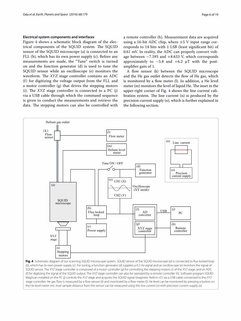
Electrical system components and interfacesFigure  4 shows a schematic block diagram of the elec-trical components of the SQUID system. The SQUID sensor of the SQUID microscope (a) is connected to an FLL (b), which has its own power supply (c). Before any measurements are made, the “Tune” switch is turned on and the function generator (d) is used to tune the SQUID sensor while an oscilloscope (e) monitors the waveform. The XYZ stage controller contains an ADC (f ) for digitizing the voltage output from the FLL and a motor controller (g) that drives the stepping motors (i). The XYZ stage controller is connected to a PC (j) via a USB cable through which the command sequence is given to conduct the measurements and retrieve the data. The stepping motors can also be controlled with

a remote controller (h). Measurement data are acquired using a 16-bit ADC chip, where ±5 V input range cor-responds to 14 bits with 1 LSB (least significant bit) of 0.61 mV. In reality, the ADC can properly convert volt-age between −7.593 and +8.633 V, which corresponds approximately to −5.8 and +6.2 μT with the post-amplifier gain of 1.

A flow sensor (k) between the SQUID microscope and the He gas outlet detects the flow of He gas, which is monitored by a flow meter (l). In addition, a He level meter (m) monitors the level of liquid He. The inset in the upper-right corner of Fig. 4 shows the line current cali-bration system. The line current (n) is produced by the precision current supply (o), which is further explained in the following section.

Helium level meter

ADconverter

XYZ stagecontroller

PC

Flow sensor

USB

Flow meter

Helium gas outlet

Power supply

Flux locked loop

SQUID microscope

CH2 (Y)

CH1 (X)Oscilloscope(XY mode)

Functiongenerator

Stepping motors

Line current

Precisoncurrent supply

XYZ stage

Tune ON / OFF

Remotecontroller

(a)

(b)

(c)

(d)

(e)

(f)

(g)

(i)

(j)

(k) (l)

(m)

(o)

(n)

(h)

Fig. 4 Schematic diagram of our scanning SQUID microscope system. SQUID sensor of the SQUID microscope (a) is connected to flux‑locked loop (b), which has its own power supply (c). For tuning, a function generator (d) supplies a 0.2‑Hz signal and an oscilloscope (e) monitors the signal of SQUID sensor. The XYZ stage controller is composed of a motor controller (g) for controlling the stepping motors (i) of the XYZ stage, and an ADC (f) for digitizing the signal of the SQUID output. The XYZ stage controller can also be operated by a remote controller (h). Software program SQUID MagScan installed on the PC (j) controls the XYZ stage and acquires the SQUID signal (magnetic field in nT) via a USB cable connected to the XYZ stage controller. He gas flow is measured by a flow sensor (k) and monitored by a flow meter (l). He level can be monitored by pressing a button on the He level meter (m). Inset sample distance from the sensor can be measured using the line current (n) with precision current supply (o)

Page 7 of 19Oda et al. Earth, Planets and Space (2016) 68:179

SQUID MagScan softwareFigure 5 shows a screen image from the SQUID micro-scope measurement and control software SQUID MagS-can. The software allows the operator to move the X- and Y-axes stepping motors of the XYZ stage. However, the Z-axis stepping motor is controlled only by the remote controller to avoid the possibility of breaking the sapphire window. The operator must register the home position of the SQUID system before starting a scan of a thin section sample. In addition, parameters such as step (mm), length (mm), and speed (mm/min) for the X- and Y-axes must be entered along with the delay [seconds (s)] between the time that the stepping motors stop and the measure-ment begins and the number of repeat measurements. A scan consists of sequential stepwise movement in the +Y direction and data acquisition followed by similar move-ment in +X direction. The operator can choose one of two scanning modes, i.e., meander (alternate between +Y and –Y directions) and one way (always in +Y direction). The analog output voltage of the FLL is digitized by the ADC of the XYZ stage controller. The gain of the meas-urement (×1, ×10, ×100, or ×500) is also input to the controller. The data from each scan are stored in a data file that contains the serial number, positions in X and Y

directions, voltage, converted magnetic field values (cal-culated using the conversion factor and the gain), and the time stamp. During a scan, the magnetic field values are color-coded and displayed in the panel in the lower-left corner of the MagScan user interface. Minimum and maximum values of the voltage and the magnetic field are displayed above the panel. If the analog voltage from the FLL exceeds the limit allowed by the ADC, the Message box displays “overscaled” in red and the message remains until the end of the scan.

Calibration and evaluationCalibration of a SQUID chipFigure 6a shows the experimental setup, including a Cir-cular Current Array System (Higuchi et al. 1989; Yoshida et  al. 1994; Adachi et  al. 2014), for the calibration of a SQUID sensor. The measurements were made in a mag-netically shielded room of two-layered PC permalloy with a shielding factor of 1/100 at 1 Hz. The Circular Current Array System is also used to determine the sensitivity and positioning of the SQUID sensor array used for mag-netoencephalography or magnetospinography (Adachi et al. 2014). The Circular Current Array System used in this study has the same setup as that shown in Fig. 1 of

Fig. 5 Screenshot of measurement software SQUID MagScan

Page 8 of 19Oda et al. Earth, Planets and Space (2016) 68:179

Adachi et al. (2014). It consists of eight 30-mm-diameter spheres on a plate and each sphere contains three coils that are perpendicular to each other. The X-, Y-, and Z-axes of the outer six spheres are parallel to each other. The three spheres in each of the outer rows are separated by 10 cm, and the two outer rows are separated by 20 cm. On the other hand, the coils on the X- and Y-axes of the inner two spheres are set at a 45° angle relative to the axes of the other six spheres. The SQUID sensor was placed ~10 cm from the inner spheres.

A precise 10-mA AC current was supplied to each coil at 80 Hz. The current control unit switched the current

from one coil to another in sequence, and the SQUID sensor voltage was measured and stored for further anal-ysis. Figure  6b presents the known parameters (normal vectors nci, position vectors rci, radius a, and current j of the magnetic field-generating coils) and the unknown parameters (normal vector ng, position vector rg, and sensitivity S of the SQUID magnetometer pickup coil) used to estimate the sensitivity of the SQUID sensor (see Higuchi et al. 1989). The best estimate of the sensitivity was 722.6 nT/V (Kawai et al. 2016). The same sensitivity is applied to all SQUID sensors with the same design fab-ricated at KIT.

Sensor‑to‑sample distance measured with a line currentA line current was used to estimate the sensor-to-sam-ple distance using a method similar to that of Fong et al. (2005). Figure  7a shows the straight 25-µm aluminum wire glued onto the glass plate that is attached to the sample holder to be scanned. The current flows from the right (blue cable) to the left (white cable) typically with a DC current of 1.000 mA.

Figure  7b shows the interface of SQUID LineScan software, which was developed using MATLAB (Math-Works, Natick, MA, USA) for estimating the distance between the SQUID sensor and the line (or sample) using data collected from the current scan. The parameters whose values are required by the software to estimate the distance are listed on the right-hand side of the software user interface and include the thickness of the sapphire window, thickness of the film on the wire and on the sam-ple, diameter of the wire, and amplitude of the current used for the scans. The polarity of SQUID, which can be flipped depending on the wiring of the SQUID chip on the sapphire rod, is also required. One set of line current scans usually includes three parallel scans 10 mm apart. Each line current scan is optimized to search for the right combination of SQUID-to-sample distance d (approxi-mately equal to half the distance between the maximum and minimum), the SQUID offset s, the conversion factor c (close to 1 if the calibration is accurate), and the posi-tion shift p along the scan direction that minimizes the difference between the line scan data and the data mod-eled according to Eq. 1:

where Bi is the magnetic field [in teslas (T)], c is the con-version factor, s is the SQUID offset, p is position shift along the y grid position, d is the distance between the line and the SQUID sensor, yi is the y grid position, y0 is the y grid position where Bi = 0, I is the current ampli-tude; and μ0 is a constant (4π × 10

−7Tm/A. The SQUID

(1)Bi = s + cµ0I

(

y0 + p+ yi)

2π

[

d2 +(

y0 + p+ yi)2]

Fig. 6 Calibration of a SQUID sensor for the SQUID microscope. a Circular Current Array System. b Schematic diagram of calibration coils and the sensor

Page 9 of 19Oda et al. Earth, Planets and Space (2016) 68:179

Fig. 7 a Line current measurement equipment. Aluminum wire (25 µm thick) is tightly stretched on a glass plate and covered with 80‑μm‑thick plastic film (not shown here). b Screenshot of the SQUID LineScan program for the calculation of sensor‑to‑sample distance

Page 10 of 19Oda et al. Earth, Planets and Space (2016) 68:179

LineScan software reports the optimized values for each line scan, an average sensor-to-sample distance, and the gap length in a vacuum (i.e., distance between the sensor and the inner wall of the sapphire window).

Figure  8 shows the conversion factor as a function of sensor-to-sample distance estimated by a series of line current scans with increasing distance. The conver-sion factor approaches 1.00 as the distance increases to ~10 mm. The discrepancy between the actual value and the theoretical value at smaller distances (i.e., the conver-sion factors are further away from 1.0) might be related to the variability of the magnetic field produced by a line current within the 200-µm ×  200-µm coil. In fact, the magnetic flux distribution of a vertical magnetic point source measured with a square SQUID loop depends on the position along the diagonal [e.g., see Figs. 20 and 21 of Granata and Vettoliere (2016)].

Noise and detection limitThe noise characteristics of the SQUID microscope sys-tem were measured at ~10-Hz intervals without moving the XYZ stage in the MSB. Figure  9a shows the back-ground noise of the SQUID magnetometer measured on July 7, 2015, from 12:00 p.m. to 1 p.m. A long-term drift component of more than 1 nT is seen together with qua-siperiodic fluctuations of about 60–90 s. Figure 9b shows the background noise measured on July 9, 2015, from 12:00 p.m. to 1 p.m. Although the quasiperiodic fluctua-tions of about 60–90 s are still observed, the drift com-ponent is less than that in Fig. 9a. The drift component might originate mainly from the change in the magnetic field of the Earth; however, long-term environmental

magnetic fields resulting from activities in the laboratory could also be a source of the drift. The 60- to 90-s qua-siperiodic component also could originate from within or near the laboratory. In addition, it is possible that the fluctuations in temperature or magnetic field are caused by air-conditioning or other components in or near the laboratory. This possibility will be investigated and improved in the future.

Figure  9c, d is expanded views of a 30-s period in Fig.  9a, b, respectively. The standard deviation of these short-period fluctuations is about 40–50  pT. Figure  9e shows the background noise of the SQUID sensor itself measured in a superconducting magnetic shield for 30 s at a sampling rate of 100 Hz with a low-pass filter (LPF) frequency of 10 Hz at KIT (Kawai et al. 2016). The stand-ard deviation of 3.0  pT is more than one order of mag-nitude smaller than that of the background noise of the SQUID microscope system. The low noise level for the SQUID sensor is achieved by the presence of the super-conducting magnetic shield, which could be the mini-mum ideal system noise in the future.

The curves in Fig.  10 indicate the detection limit of a vertical dipole pointing up or down with a magnetic moment of 1 ×  10−14 Am2 (blue line), 1 ×  10−15 Am2 (yellow line), or 1 ×  10−16 Am2 (purple line), assuming that 100 pT is the minimum noise level (see Fig. 9c, d). For the typical sensor-to-sample distance (i.e., ~200 µm) in current SQUID system, a magnetic moment of 1 × 10−14 Am2 can be detected if the long-term drift and 60- to 90-s quasiperiodic fluctuations are reduced and compensated. Considering the typical scanning interval ([X,Y] =  [100  µm ×  100  µm]) and the scanning rate of ~0.36 s/point (e.g., number of points [X,Y] = [651, 301], delay time before data acquisition [0.1 s], speed of motor [X,Y] = [100 mm/min., 100 mm/min.], time from start to end [70,440 s]), one scan line in Y direction takes ~108 s. This is shorter than the typical wave lengths of long-term drift observed in Fig. 9c, d, which can be reduced by the drift correction assuming linear drift and zero magnetic field at start and end of each line. For a stoichiometric magnetite (saturation magnetization = ~4.8 × 105 A/m), a magnetic moment of 1 ×  10−14 Am2 corresponds to an ~275-nm cube of magnetite. Reducing the sensor-to-sample distance to 100  µm allows detection of a mag-netic moment of 1 ×  10−15 Am2, which corresponds to an ~128-nm cubic magnetite. This sensitivity is compa-rable to the best possible moment sensitivity of >10−15 Am2 estimated by Weiss et  al. (2007a) for their SQUID microscope with a sensor-to-sample distance of 100 µm. Further, if we achieve 1 × 10−16 Am2 corresponding to an ~59-nm cube of magnetite, it is enough for most paleomagnetic studies because the SP/SD boundary of magnetite is around 15–50 nm (e.g., Newell and Merrill

Senour-to-Sample Distance (mm)

Con

vers

ion

Fact

or

Fig. 8 Conversion factor as a function of sensor‑to‑sample distance. Error bar represents standard deviation of three values of sensor‑to‑sample distances calculated for lines 1 through 3

Page 11 of 19Oda et al. Earth, Planets and Space (2016) 68:179

Standard deviation = 3.0 pT

Standard deviation = 53.1 pT

Standard deviation = 40.4 pT

a

b

c

d

e

Fig. 9 Background noise of SQUID magnetometer measured on a July 7, 2015, and b July 9, 2015, for 1 h. In both recordings, a long‑term drift com‑ponent (>1 nT in a) is seen together with the periodic fluctuations of about 60–90 s. c, d Expanded 30‑s measurement from a and b, respectively. e Background noise of the SQUID sensor itself measured in a superconducting magnetic shield for 30 s at a sampling rate of 100 Hz with an LPF of 10 Hz

Page 12 of 19Oda et al. Earth, Planets and Space (2016) 68:179

1999). On the other hand, we may need to think about the stability of magnetic moment carried by a sample with small magnetic moment (Berndt et al. 2016). Kirsch-vink et  al. (2015) reported the best sensitivity for a 2G SRM is ~10−13 Am2 using ultraclean quartz glass sam-ple holder. The measurement of a small specimen, such as a magnetic inclusion in a single crystal (e.g., Sato et al. 2015; Tarduno et  al. 2015), can be improved by using a SQUID microscope for measuring the magnetic moment. Recently, Lima and Weiss (2016) demonstrated that their SQUID microscope could measure a magnetic dipole moment down to about 10−15 Am2.

Precision of the XY stage positioningTo evaluate the repeatability and accuracy of the sample positioning of the XYZ stage, we performed laser inter-ferometry (Fig.  11a) with the laser encoder unit RLU10 (Renishaw plc, Gloucestershire, UK), similar to the meas-urements conducted by Oda et  al. (2016b). The laser beam reflector (RLR10-A3-XF) was attached to the sam-ple table, and the laser detector head (RLD 90° RRI) was tightly affixed to a tripod on the floor. While the sample table of the XYZ stage was moving, the Y positions were monitored and recorded (the photograph in Fig.  11a is taken in the X direction for demonstration). The meas-urements were adjusted for the environmental conditions with temperature of 24°C, humidity of 46%, and atmos-pheric pressure of 99.86 kPa.

The plots in Fig.  11b show the difference between the position setting of the XYZ stage and the position

determined by laser interferometry for the first (solid symbols) and second (open symbols) measurements. With the X-axis position fixed, the XYZ stage was moved in +Y direction (blue symbols) from the starting position (zero) to 50  mm in 1-mm steps and then in –Y direc-tion (red symbols) back to the original position in 1-mm steps. There was a systematic increase (in +Y direction) or decrease (in –Y direction) of about 0.15 mm in the dif-ference between the set position of the XYZ stage and that measured by laser interferometry at 50  mm. This increase or decrease corresponds to a 0.3% systematic

Noise level of SQUID microscope (minimum)

Noise level of SQUID sensor

Current Distance

Target Distance

Ver

tical

Mag

netic

Fie

ld (n

T)

Fig. 10 Detection limit expected for a magnetic dipole. Magnetic fields produced just above a vertical magnetic dipole with mag‑netic moments of 1 × 10−14 Am2 (blue), 1 × 10−15 Am2 (yellow), and 1 × 10−16 Am2 (purple) are plotted versus distance. Red dashed vertical lines are the current sensor‑to‑sample distance (200 µm) and the target distance (100 µm), respectively. Minimum estimates of the noise level of the SQUID microscope system and the SQUID sensor are indicated by black horizontal dashed lines

0.15

0.10

0.05

0.00

)m

m(egna

RresaL-gnitteS

noitisoP

50403020100Position (mm)

+Y 1st -Y 1st +Y 2nd -Y 2nd

a

b

Fig. 11 a Experimental setup for laser interferometry measurement of the XYZ stage positioning. b Results of laser interferometry. X‑axis stepping motor was fixed, and the Y‑axis stepping motor was moved in 1‑mm steps according to the software. Blue solid (open) circles plot the difference between the XYZ stage position setting and the posi‑tion measured with laser interferometry in +Y direction for the first (second) measurement, and the red solid (open) circles are for the −Y direction measurements

Page 13 of 19Oda et al. Earth, Planets and Space (2016) 68:179

error or a 0.3° deflection of the axis of the light relative to the Y-axis of the XYZ stage. In all cases, the random error of the Y position was less than ±0.01 mm. The system-atic difference of ~0.03  mm between the +Y measure-ments (blue) and the −Y measurements (red) might have been caused by backlash from a ball screw contacting a ball nut. In conclusion, spacial resolution of the system is ~200 µm, considering the size of pick-up coil, sensor-to-sample distance, and the accuracy of XYZ stage discussed above.

Two‑axis tumbling AF demagnetization system for thin section samplesFigure  12a shows the specially designed tumbler that rotates a thin section sample along two axes simultane-ously during AF demagnetization. A thin section is cov-ered with cotton for protection and is placed diagonally in the plastic inner rotator (the semitransparent piece on the left). The rotation axis of the inner rotator is sup-ported by the two blue stands on the outer rotator. The spin of the motor beneath the blue pulley (left-hand side of Fig. 12b) is transmitted to the outer rotator via a ure-thane belt (dark orange component in Fig.  12b). While

the outer rotator spins along vertical axis, the inner rota-tor spins along the horizontal axis via the fixed circular pad (light brown piece in the outer rotator in Fig.  12a) that touches the thin urethane belt around the outside of the inner rotator. The tumbler rotates the thin section along two axes simultaneously at different rates, result-ing in the random positioning of the thin section during AF demagnetization. AF demagnetization up to 100 mT was performed using AF demagnetizer model DEM-95C (Natsuhara Co. Ltd.) with a three-layered PC permalloy shield in a residual magnetic field of ~10 nT.

Magnetic image registration using paired point sourcesPrinciplesIt is usually not difficult to correlate positions on opti-cal and electron microscopic images of thin sections. On the other hand, it is difficult to correlate the positions on those images with a magnetic image because the latter is blurred due to the distance from the magnetic source and is shifted horizontally depending on the direction of magnetization. Fong et al. (2005) demonstrated the reg-istration of a magnetic image with a photographic image by using two line currents that perpendicularly crossed each other. Two crossed wires were placed on the sample holder after removing the thin section, and the magnetic image was taken. The magnetic image of a thin section was matched to that produced by the two crossed lines, which correlated with the optical images of the lines and with the optical image of the thin section. This method is effective for registering images; however, the magnetic measurement of the two crossed line currents requires additional setup and is time-consuming. Thus, we have developed an alternative method that uses two point sources placed diagonally on the sample holder outside of the thin section. The advantage of this method is that the sample and the point sources can be scanned at the same time.

Demonstration of image registrationA thin section of an Hawaiian basalt was pressed upside down onto the glass window of a flatbed optical color scanner (EPSON GT-X980 with a resolution of 6400 dpi × 6400 dpi and pixel size = 4 μm × 4 μm), covered with a thin transparent film for protection, and scanned using reflected light (Fig. 13a). The sample holder has two holes to anchor the point sources. We fabricated a sput-tered FeCo circle, 75 µm in diameter and 500 nm thick, on a Si substrate (see an optical microscopic image in Fig. 13e). Because each point source is fabricated in the middle of the Si chip, the center of the Si chip (Fig. 13a; point where the yellow lines cross) represents the posi-tion of the point source. Because the point sources are

Fig. 12 a Sample holder and tumbler that enables rotation of a thin section sample along two axes simultaneously during AF demagneti‑zation. b Sample holder and tumbler prepared for AF demagnetiza‑tion

Page 14 of 19Oda et al. Earth, Planets and Space (2016) 68:179

c

b

a

X

Y

Z

fed

27.5

27.0

26.5

26.0

)m

m(Y

63.563.062.562.061.5X (mm)

-40

-20

0

20

40

nT

0.5mm

3.5

3.0

2.5

2.0

)m

m(Y

3.53.02.52.0X (mm)

-800

-400

0

400

800

nT

0.5mm

0.2mm

Page 15 of 19Oda et al. Earth, Planets and Space (2016) 68:179

flat disks, they can be easily magnetized in the horizontal direction.

Figure 13b shows the magnetic image of natural rema-nent magnetization (NRM) of the basalt sample meas-ured after AF demagnetization at 20 mT peak field. The color bar on the right gives the magnetic field values in nT; e.g., red and blue correspond to positive and negative values, respectively. We applied linear drift correction for the raw data assuming averages of the first and the last ten measurements (above and below the two horizon-tal broken lines in Fig. 13b) for each line scan in the +Y direction (starting at 0 mm and ending at 50 mm) should be adjusted to zero. Figure  13c overlays the magnetic image in Fig.  13b on the optical image in Fig.  13a after conversion to a gray-scale image. Leakage of the mag-netic field in the bubble holes within the sample and out-side of the sample can be observed.

To register the magnetic image relative to the optical image, the positions of the point sources are calculated by fitting the dipolar magnetic field to the theoretical distribution of a dipole. Figure  13d is an enlargement (2  mm  ×  2  mm) of the magnetic image produced by point source A on the lower-left corner in Fig.  13b. To eliminate the noise from sources other than the point sources (e.g., dust particles), the magnetic data from only within 0.8  mm (the distance limit parameter can be changed) of the expected center (i.e., the midpoint of the maximum and the minimum for a horizontal dipole) were used to fit the data. We used the “Curve fitting” feature of the program IGOR Pro (WaveMetrics, Inc., Lake Oswego, OR, USA) to find the best dipole fit. A user-defined function in IGOR Pro produced a vertical magnetic field for a magnetic dipole calculated using the following formula:

where r = (x,y,z) − (x0,y0,z0) and m = (mx,my,mz), where (x,y,z) is the measurement position, (x0,y0,z0) is the dipole position, and (mx,my,mz) is the magnetic moment of a dipole. A nonlinear least-squares data fit using the Levenberg–Marquardt algorithm was used to search for the minimum value of residual sum of squares. An initial guess for (x0,y0) was the midpoint between the

(2)B(r) =µ0

4π ||r||3

(

3r(m · r)

||r||2−m

)

maximum and minimum for an assumed horizon-tal dipole, which is located manually using a cursor on the horizontal map. An initial guess for the z0 position (depth) was set at −0.3 mm (approximately the sensor-to-sample distance), and mx, my, and mz were set to zero.

The search for the minimum value of residual sum of squares began by traveling downhill from the start-ing point on the surface of residual sum of squares. We conducted several “Curve fitting”s with the default of 40 iterations, where each “Curve fitting” started with the previously estimated optimum values until no improve-ment was observed.

The contours in Fig.  13f represent the magnetic field produced by an optimized magnetic dipole after a non-linear least-squares fit. The red cross (x) in the center indicates the estimated position of the dipole on the XY plane. Figure 13f is an enlargement of the magnetic field produced by point source B in the upper-right corner of Fig. 13b. Because the Si chip of point source B was placed upside down, the signal is smaller and broader than that of the point source A.

Table 1 gives the results of the magnetic dipole fitting of the two point sources for six consecutive measurements of a basalt thin section. All X and Y positions were meas-ured relative to a fixed home position. The standard devi-ation of the Y position was ~0.5 mm for the X-axis and ~0.35  mm for the Y-axis. The vertical distance of point sources A and B from the sensor was 0.29 ± 0.02 mm and 0.91 ± 0.16 mm, respectively. The difference in the verti-cal distance was due to point accidentally placing source B underneath the Si chip, which was ~0.5 mm thick. The standard deviation of the difference in the X and Y posi-tions of the two point sources was 0.09 and 0.10  mm, respectively. The results indicate that the relatively large standard deviation of the estimated horizontal position might be caused not by calculation error but by the rela-tive shift between the sample holder and the thin section, because a rubber cylinder presses the sample in a slightly different manner on each sample change (see circular component in the lower-right corner of Fig. 13a).

Figure  14a–d demonstrates the change in the mag-netic image depending on the direction of magnetiza-tion of a thin section. Figure  14a is the magnetic image after subjecting a thin section to anhysteretic remanent

(See figure on previous page.) Fig. 13 Registration of a magnetic image with an optical image using two point sources. Sensor‑to‑sample distance was 216 µm when the magnetic field was measured. a Optical scanner image of a basalt thin section sample with two point sources on the corners. b Magnetic image of the same sample with NRM after 20‑mT AFD. c Magnetic image overlaid on the gray‑scaled optical image. d The image is an enlargement of the magnetic field produced by point source A placed in the lower‑left corner of b outside of a thin section. The contours represent the magnetic field estimated for an optimized magnetic dipole after a nonlinear least‑squares fit. The red cross in the center indicates the estimated position of the dipole on the XY plane. e Optical microscopic image of a 75‑µm φ point source made of FeCo on a Si square substrate. f The image is an enlarge‑ment of the magnetic field produced by point source B in the upper‑right corner of b. Explanations on contours and the red cross are the same as d

Page 16 of 19Oda et al. Earth, Planets and Space (2016) 68:179

Tabl

e 1

Para

met

ers

for a

pai

r of p

oint

sou

rces

use

d in

 regi

ster

ing

mag

neti

c im

age

rela

tive

to o

ptic

al im

age

Erro

r mea

ns th

e er

ror e

xpec

ted

for t

he p

ositi

on o

ptim

ized

by

mag

netic

imag

e as

sum

ing

a m

agne

tic d

ipol

e

A lo

wer

-left

poi

nt s

ourc

e, B

upp

er-r

ight

poi

nt s

ourc

e, D

iffer

ence

sub

trac

ted

A fr

om B

STD

sta

ndar

d de

viat

ion,

M in

tens

ity o

f mag

netic

mom

ent

dec

decl

inat

ion

(clo

ckw

ise

from

+x

dire

ctio

n), i

nc in

clin

atio

n (p

ositi

ve fo

r low

er h

emis

pher

e)

Poin

t sou

rce

X (m

m)

Erro

r (1σ

)Y

(mm

)Er

ror (

1σ)

Z (m

m)

Erro

r (1σ

)M

(Am

2 )Er

ror (

1σ%

)D

ec (°

)Er

ror (

1σ)

Inc

(°)

Erro

r (1σ

)

AN

RM3.

803

0.00

22.

694

0.00

3−

0.26

60.

003

2.04

E−10

2.8

171.

50.

7−

2.1

0.7

AFD

10

mT

2.37

00.

001

2.55

50.

001

−0.

264

0.00

12.

13E−

100.

917

1.3

0.2

0.2

0.2

AFD

20

mT

2.75

60.

002

2.63

80.

002

−0.

213

0.00

32.

03E−

101.

017

1.0

0.3

0.4

0.3

ARM

(+X)

2.51

90.

001

2.25

90.

001

−0.

275

0.00

12.

16E−

100.

817

1.2

0.2

0.1

0.2

ARM

(+Y)

2.73

70.

002

2.03

50.

003

−0.

280

0.00

32.

27E−

102.

417

0.6

0.6

0.3

0.6

ARM

(−Z)

2.66

90.

002

1.83

90.

002

−0.

258

0.00

22.

20E−

101.

916

8.6

0.4

1.1

0.5

Ave

rage

2.80

92.

336

−0.

259

2.14

E−10

STD

0.50

90.

349

0.02

49.

22E−

12

BN

RM63

.702

0.00

227

.048

0.00

2−

0.75

70.

003

2.50

E−10

1.2

97.4

0.2

−2.

32.

0

AFD

10

mT

62.2

00.

005

26.8

310.

004

−0.

881

0.00

72.

65E−

101.

999

.10.

4−

2.1

0.3

AFD

20

mT

62.6

780.

005

26.7

540.

005

−1.

032

0.00

92.

75E−

102.

299

.60.

4−

3.4

0.3

ARM

(+X)

62.3

450.

007

26.4

800.

006

−1.

204

0.01

23.

08E−

102.

799

.80.

5−

6.0

0.4

ARM

(+Y)

62.4

760.

003

26.2

090.

002

−0.

831

0.00

42.

57E−

101.

397

.40.

2−

3.0

0.2

ARM

(−Z)

62.6

570.

003

26.1

890.

004

−0.

772

0.00

42.

48E−

101.

397

.10.

3−

2.9

0.2

Ave

rage

62.6

7726

.585

−0.

913

2.67

E−10

STD

0.53

40.

350

0.17

42.

24E−

11

Diff

eren

ceN

RM59

.899

24.3

54−

0.49

1

AFD

10

mT

59.8

3324

.276

−0.

617

AFD

20

mT

59.9

2224

.116

−0.

819

ARM

(+X)

59.8

2624

.221

−0.

929

ARM

(+Y)

59.7

3924

.174

−0.

552

ARM

(−Z)

59.9

8824

.350

−0.

514

Ave

rage

59.8

6824

.249

−0.

654

STD

0.08

70.

096

0.17

9

Page 17 of 19Oda et al. Earth, Planets and Space (2016) 68:179

magnetization (ARM) (DC 50 µT, AC 80 mT) in the +X direction. Figure  14b is the result of overlaying Fig.  14a on the gray-scaled optical scanner image. The positive magnetic field is observed on the right-hand side of the sample optical image and the negative magnetic field on the left-hand side. This is consistent with the direction of sample magnetization. Figure 14c is the magnetic image after subjecting a thin section to the same ARM as in Fig. 14a but in the −Z direction. Figure 14d is the result

of overlaying Fig. 14c on the gray-scaled optical scanner image.

Magnetic field leaks outside of the sample area or in the bubble holes appear as positive values in general, which is consistent with the overall negative magnetization of a sample. These results demonstrate the successful appli-cation of our new method of registering a thin section sample using a pair of point sources placed on the sample holder.

a ARM (+X) ; magnetic image

c ARM (-Z) ; magnetic image

b ARM (+X) ; overlay image

d ARM (-Z) ; overlay image

10 mm10 mm

10 mm10 mmX

Y

Z

X

Y

Z

nTnT

Fig. 14 Magnetic images after subjecting the thin section sample to ARM with a DC field of 50 µT and an AC field of 80 mT. a Magnetic image of ARM in the +X direction. b Image in a overlaid on the optical scanner image. c Magnetic image of ARM in the −Z direction. d Image in c overlaid on the optical scanner image. Color scale represents the vertical magnetic field in nT (positive upward)

Page 18 of 19Oda et al. Earth, Planets and Space (2016) 68:179

ConclusionsWe developed a scanning SQUID microscope system for imaging the vertical component of a magnetic field on the surfaces of geological samples at room tem-perature. The system comprises a SQUID microscope, a magnetically shielded box (MSB), an XYZ stage, and auxiliary electronic equipment. The SQUID sensor is a washer-type pick-up coil with 200 μm × 200 μm, which has an inner hole of 30 μm × 30 μm. The SQUID micro-scope can operate up to 4 days on 10 L of liquid He. The MSB is made of two-layered PC permalloy with shield-ing factors of 1/257, 1/288, and 1/91 in the X, Y, and Z directions, respectively. The DC component of residual magnetic field at the measurement position was less than 5 nT. The non-magnetic XYZ stage with its 80-cm neck is driven by three-axis stepping motors under-neath the MSB. The stroke of the XYZ stage is 100 mm in the X and Y directions and has an accuracy of ~10 µm confirmed by laser interferometry. The easy-to-use graphical software SQUID MagScan controls the XYZ stage and digitizes the analog voltage output from the FLL connected to SQUID sensor while scanning a thin section.

A Circular Current Array System calibrated the sensi-tivity of the SQUID sensor as 722.6 nT/V. The sensor-to-sample distance was estimated by scanning a precision line current and analyzing the results using the devel-oped SQUID LineScan software. We achieved the mini-mum sensor-to-sample distance of ~200  µm by using a 50-μm-thick sapphire window and a 40-µm thin protec-tive film on a thin section sample. Considering the size of pick-up coil, sensor-to-sample distance, and the accu-racy of XYZ stage, spacial resolution of the system is ~200 µm. The minimum noise level of a SQUID micro-scope is expected to be ~100  pT, excluding long-term drift and fluctuations, which is more than an order of magnitude larger than that of a SQUID sensor (~3 pT). With the current minimum sensor-to-sample distance of ~200 µm and a minimum noise level of ~100 pT, a mag-netic dipole with a magnetic moment of 1 × 10−14 Am2 can be detected; this corresponds to an ~275-nm cube of magnetite.

We proposed a new method for registering a magnetic image with an optical image that uses a pair of point sources placed diagonally on the sample holder outside of the thin section sample. We performed six successful demonstrations of this method using a basalt thin sec-tion and found a standard deviation of ~0.1  mm for a distance (x 59.9 mm, y 24.2 mm) between the two point sources. Magnetic images of the NRM and ARM over-laid on the gray-scaled optical image are comprehensive and could be used for further analysis, modeling, and interpretation.

AbbreviationsAC: alternating current; ADC: analog‑to‑digital converter; AF: alternating field; AIST: National Institute of Advanced Industrial Science and Technology; ARM: anhysteretic remanent magnetization; DC: direct current; FLL: flux‑locked loop; GFRP: glass fiber‑reinforced plastics; GSJ: Geological Survey of Japan; KIT: Kanazawa Institute of Technology; LPF: low‑pass filter; LSB: least significant bit; NRM: natural remanent magnetization; SQUID: superconducting quantum interference device; SRM: SQUID rock magnetometer.

Authors’ contributionsHO designed and developed the entire system and wrote and edited most of the manuscript; JK developed the SQUID sensor and designed the sap‑phire window and rod and other components of the SQUID microscope; MM developed the electronics (FLL) for the SQUID sensor; IM designed the sample holder; MS conducted measurements and interpreted the results; AN conducted measurements and maintenance; YY conducted measurements on the range of the laser and provided the samples; JF developed the cryostat for the SQUID microscope; NN designed and developed the XYZ stage and tumbler; YA developed the XYZ stage controller and data acquisition software; TM designed the magnetic shield box; CX developed the software for the analysis of the line scan data and edited the manuscript. All authors read and approved the final manuscript.

Author details1 Research Institute of Geology and Geoinformation, Geological Survey of Japan, AIST, Central 7, 1‑1‑1 Higashi, Tsukuba 305‑8567, Japan. 2 Applied Electronics Laboratory, Kanazawa Institute of Technology, Kanazawa 920‑1331, Japan. 3 Research Institute of Earthquake and Volcano Geology, Geologi‑cal Survey of Japan, AIST, Central 7, 1‑1‑1 Higashi, Tsukuba 305‑8567, Japan. 4 Center for Advanced Marine Core Research, Kochi University, B200 Monobe, Nankoku, Kochi 783‑8502, Japan. 5 Fujihira Co. Ltd., Tsukuba 305‑0047, Japan. 6 Natsuhara Giken Co. Ltd., Osaka 532‑0033, Japan. 7 Ayzy Co. Ltd., Kyoto 616‑8312, Japan. 8 Ohtama Co., Ltd., 1744 Oshitate, Inagi, Tokyo 206‑0811, Japan. 9 School of Ocean and Earth Science, National Oceanogra‑phy Centre Southampton, University of Southampton, Waterfront Campus, European Way, Southampton SO14 3ZH, UK.

AcknowledgementsHirokuni Oda was supported by a JSPS Grant‑in‑Aid for Scientific Research (A) (Funding No. 25247073). Chuang Xuan is supported by a startup fund provided by the University of Southampton. JSPS provided a Visiting Fellow‑ship for Foreign Researchers (Award No. PE14034) for Chuang Xuan to visit the Geological Survey of Japan (GSJ), a part of the National Institute of Advanced Industrial Science and Technology (AIST), to conduct work related to this research. The authors are indebted to Norihiro Nakamura, Yoichi Usui, and Akira Usui for contributing to the discussions on the system. The magneti‑cally shielded box, sapphire rod with metalized wire, and sapphire window were made by Ohtama Co., Ltd., Kyocera Corporation, and Ceraken Co., Ltd., respectively. Tomomi Kobayashi helped in the development of convenient tools necessary for the SQUID microscope system. The authors thank Ayako Katayama for performing the measurements with the scanning SQUID micro‑scope system and producing the artwork. The authors thank Miki Kawabata for fabricating and evaluating the SQUID chips. The manuscript was improved by the positive comments of the two anonymous reviewers and the editor.

Competing interestsThe authors declare that they have no competing interests.

Received: 30 July 2016 Accepted: 15 October 2016

ReferencesAdachi Y, Higuchi M, Oyama D, Haruta Y, Kawabata S, Uehara G (2014) Calibra‑

tion for a multichannel magnetic sensor array of a magnetospinography system. IEEE Trans Magn 50:5001304

Baudenbacher F, Peters NT, Wikswo JP Jr (2002) High resolution low‑temper‑ature superconductivity superconducting quantum interference device microscope for imaging magnetic fields of samples at room temperature. Rev Sci Instrum 73:1247–1254

Page 19 of 19Oda et al. Earth, Planets and Space (2016) 68:179

Baudenbacher F, Fong LE, Holzer JR (2003) Monolithic low‑transition‑tempera‑ture superconducting magnetometers for high resolution imaging mag‑netic fields of room temperature samples. Appl Phys Lett 82:3487–3489

Berndt T, Muxworthy AR, Fabian K (2016) Does size matter? Statistical limits of paleomagnetic field reconstruction from small rock specimens. J Geo‑phys Res Solid Earth 121:15–26. doi:10.1002/2015JB012441

Chatraphorn S, Fleet EF, Wellstood FC (2000) Scanning SQUID microscopy of integrated circuits. Appl Phys Lett 76:2304–2306

Constable C, Parker R (1991) Deconvolution of longcore palaeomagnetic measurements—spline therapy for the linear problem. Geophys J Int 104:453–468. doi:10.1111/j.1365‑246X.1991.tb05693.x

Fischer WW, Fike DA, Johnson JE, Raub TD, Guan Y, Kirschvink JL, Eiler JM (2014) SQUID–SIMS is a useful approach to uncover primary signals in the Archean sulfur cycle. Proc Natl Acad Sci 111:5468–5473. doi:10.1073/pnas.1322577111

Fong LE, Holtzer JR, McBride KK, Lima EA, Baudenbacher F (2005) High‑reso‑lution room‑temperature sample scanning superconducting quantum interference device microscope configurable for geological and biomag‑netic applications. Rev Sci Instrum 76:053703

Fu RR, Weiss BP, Lima EA, Harrison RJ, Bai XN, Desch SJ, Ebel DS, Suavet C, Wang H, Glenn D, Sage DL, Kasama T, Walsworth RL, Kuan AT (2014) Solar nebula magnetic fields recorded in the Semarkona meteorite. Science 346:1089–1092. doi:10.1126/science.1258022

Fu RR, Weiss BP, Lima EA, Kehayias P, Araujo JFDF, Glenn DR, Gelb J, Einsle JF, Bauer AM, Harrison RJ, Ali GAH, Walsworth RL (2016) Evaluating the paleomagnetic potential of single zircon crystals using the Bishop Tuff. Earth Planet Sci Lett. doi:10.1016/j.epsl.2016.09.038

Gattacceca J, Boustie M, Weiss BP, Rochette P, Lima EA, Fong LE, Baudenbacher FJ (2006) Investigating impact demagnetization through laser impacts and SQUID microscopy. Geology 34:333–336. doi:10.1130/G21898.1

Granata C, Vettoliere A (2016) Nano superconducting quantum interference device: a powerful tool for nanoscale investigations. Phys Rep 614:1–69. doi:10.1016/j.physrep.2015.12.001

Higuchi M, Chinone K, Ishikawa N, Kado H, Kasai N, Nakanishi M, Koyanagi M, Ishibashi Y (1989) The positioning of magnetometer pickup coil in dewar by artificial signal source. In: Wiliamson SJ (ed) Advances in biomag‑netism. Plenum Press, New York, pp 701–704

Jackson M, Bowles JA, Lascu I, Solheid P (2010) Deconvolution of u channel magnetometer data: experimental study of accuracy, resolution, and stability of different inversion methods. Geochem Geophys Geosyst 11:Q07Y10. doi:10.1029/2009GC002991

Kawai J, Oda H, Fujihira J, Miyamoto M, Miyagi I, Sato M (2016) SQUID microscope with hollow‑structured cryostat for magnetic field imaging of room temperature samples. IEEE Trans Appl Supercond 26:1600905. doi:10.1109/TASC.2016.2536751

Kirschvink JL, Isozaki Y, Shibuya H, Otofuji Y, Raub TD, Hilburn IA, Kasuya T, Yokoyama M, Bonifacie M (2015) Challenging the sensitivity limits of paleomagnetism: magnetostratigraphy of weakly magnetized Guadalu‑pian–Lopingian (Permian) limestone from Kyushu, Japan. Palaeogeogr Palaeoclimatol Palaeoecol 418:75–89

Kirtley JR, Wikswo JP Jr (1999) Scanning SQUID microscopy. Annu Rev Mater Sci 29:117–148

Lima EA, Weiss BP (2016) Ultra‑high sensitivity moment magnetometry of geo‑logical samples using magnetic microscopy. Geochem Geophys Geosyst. doi:10.1002/2016GC006487

Lima EA, Bruno AC, Carvalho HR, Weiss BP (2014) Scanning magnetic tunnel junction microscope for high‑resolution imaging of remanent magneti‑zation fields. Meas Sci Technol 25:105401

Newell AJ, Merrill RT (1999) Single‑domain critical sizes for coercivity and remanence. J Geophys Res 104(B1):617–628. doi:10.1029/1998JB900039

Oda H, Xuan C (2014) Deconvolution of continuous paleomagnetic data from pass‑through magnetometer: a new algorithm to restore geomagnetic

and environmental information based on realistic optimization. Geo‑chem Geophys Geosyst 15:3907–3924. doi:10.1002/2014GC005513

Oda H, Usui A, Miyagi I, Joshima M, Weiss BP, Shantz C, Fong LE, McBride KK, Harder R, Baudenbacher F (2011) Ultrafine‑scale magnetostratigraphy of marine ferromanganese crust. Geology 39:227–230

Oda H, Miyagi I, Kawai J, Suganuma Y, Funaki M, Imae N, Mikouchi T, Matsuzaki T, Yamamoto Y (2016a) Volcanic ash in bare ice south of Sor Rondane Mountains, Antarctica: geochemistry, rock magnetism and nondestruc‑tive magnetic detection with SQUID gradiometer. Earth Planets Space 68:39. doi:10.1186/s40623‑016‑0415‑3

Oda H, Xuan C, Yamamoto Y (2016b) Toward robust deconvolution of pass‑through paleomagnetic measurements: new tool to estimate mag‑netometer sensor response and laser interferometry of sample position‑ing accuracy. Earth Planets Space 68:109. doi:10.1186/s40623‑016‑0493‑2

Ono Y, Ishiyama A (2004) Development of biomagnetic measurement system for mice with high spatial resolution. Appl Phys Lett 85:332–334

Sato M, Yamamoto S, Yamamoto Y, Okada Y, Ohno M, Tsunakawa H, Maruyama S (2015) Rock‑magnetic properties of single zircon crystals sampled from the Tanzawa tonalitic pluton, central Japan. Earth Planets Space 67:150. doi:10.1186/s40623‑015‑0317‑9

Tarduno JA, Cottrell RD, Davis WJ, Nimmo F, Bono RK (2015) A Hadean to Paleoarchean geodynamo recorded by single zircon crystals. Science 349:521–524. doi:10.1126/science.aaa9114

Wang Q, Qin H, Liu Q, Song T (2014) Room temperature sample scanning SQUID microscope for imaging the magnetic fields of geological speci‑mens. Appl Mech Mater 475–476:3–6

Weiss BP, Kirschvink JL, Baudenbacher FJ, Vali H, Peters NT, Macdonald FA, Wikswo JP Jr (2000) A low temperature transfer of ALH84001 from Mars to Earth. Science 290:791–795

Weiss BP, Lima EA, Fong L, Baudenbacher F (2007a) Paleomagnetic analysis using SQUID microscopy. J Geophys Res 112:B09105

Weiss BP, Lima EA, Fong LE, Baudenbacher F (2007b) Paleointensity of the Earth’s magnetic field using SQUID microscopy. Earth Planet Sci Lett 264:61–71

Xuan C, Oda H (2015) UDECON: deconvolution optimization software for restoring high‑resolution records from pass‑through paleo‑magnetic measurements. Earth Planets Space 67:183. doi:10.1186/s40623‑015‑0332‑x

Yoshida T, Higuchi M, Komuro T, Kado H (1994) Calibration system for a multichannel SQUID magnetometer. In: Proceedings of the 16th annual international conference of IEEE engineering in medicine and biology society. Engineering advances: new opportunities for biomedical engi‑neers, November 1994, pp 171–172