Section 5 Molecular Electronic Spectroscopy

Section 5 Molecular Electronic SpectroscopyMolecular Electronic Spectroscopy

(lecture 9 ish)Molecular Electronic Spectroscopy

(lecture 9 ish)

Quantum theoryPreviously: Quantum V l

Q yof atoms / molecules

Previously:

Molecular Electronic Spectroscopy

QMechanics

Valence

Molecular Electronic SpectroscopyClassification of electronic statesMolecular termsElectronic transitions: The Franck‐Condon PrincipleElectronic transitions: The Franck Condon PrincipleFranck‐Condon factorsVibrational structure: Birge‐Sponer extrapolationRotational structure: BandheadsIntroduction to photoelectron spectroscopy

Molecular l

Molecular lEnergy LevelsEnergy Levels

i.e., typically ΔEel >> ΔEvib >> ΔErot

Different electronic states (electronic arrangements)(electronic arrangements)

λΔ ≈

≈E 2 x 104 – 105 cm‐1

500 – 100 nm

102 – 5 x 103 cm‐1

100 μm – 2 μm

3 – 300 GHz (0.1 – 10 cm‐1)

Transitions at λVis – UV 

00 μ μinfrared

10 cm – 1 mmmicrowave

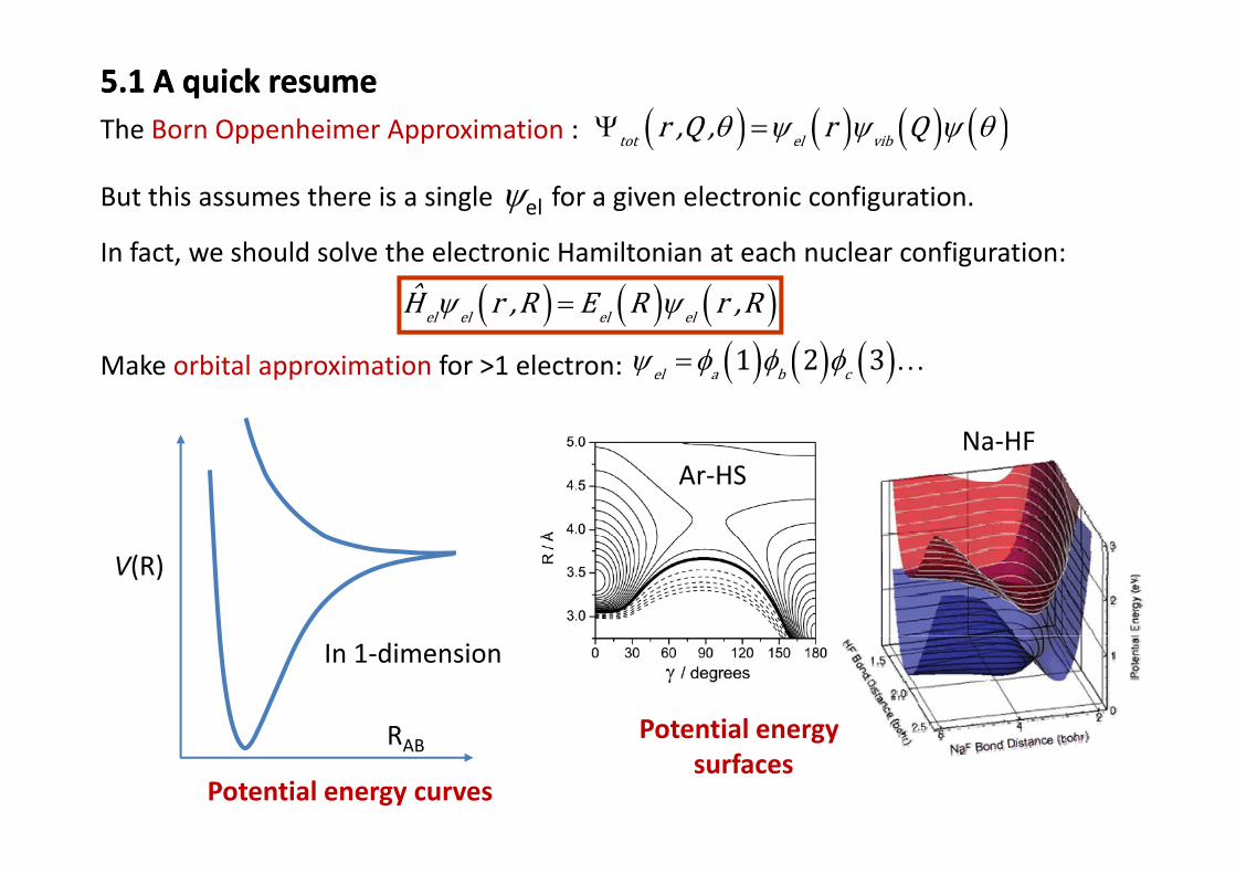
5.1 A quick resume5.1 A quick resume( ) ( ) ( ) ( )tot el vibr ,Q , r Qθ ψ ψ ψ θΨ =The Born Oppenheimer Approximation : ( ) ( ) ( ) ( )tot el vib,Q , Qψ ψ ψpp pp

But this assumes there is a single ψel for a given electronic configuration. 

In fact, we should solve the electronic Hamiltonian at each nuclear configuration:

( ) ( ) ( )el el el elH r ,R E R r ,Rψ ψ=

Make orbital approximation for >1 electron:  ( ) ( ) ( )1 2 3el a b cψ φ φ φ= …

Na HFAr‐HS

Na‐HF

V(R)

Potential energyR

In 1‐dimension

Potential energy curves

Potential energy surfaces

RAB

5.2 Classifying molecular electronic states5.2 Classifying molecular electronic states

Diatomic Term SymbolsDiatomic Term Symbols:Classify according to angular momentum around the internuclear axis, λ.

λ is analogous to ml in atoms: 

e.g., a p orbital has l = 1, ml = 0, ±1  

Two p‐orbital systems yield σ and π molecular orbitals; 

pz (ml=0) combine to yield σ, σ∗ (λ=0) +

px,y (ml= ±1) combine to yield π, π∗ (λ=±1)+

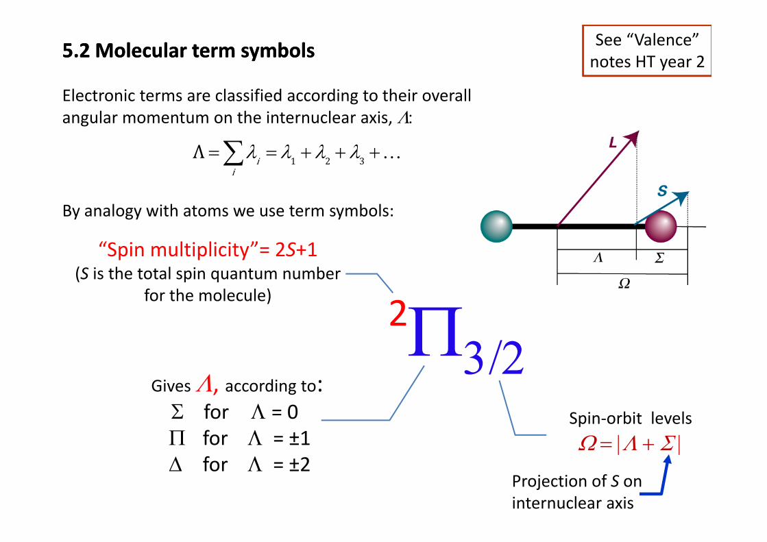
5.2 Molecular term symbols5.2 Molecular term symbols See “Valence” notes HT year 2

Electronic terms are classified according to their overall angular momentum on the internuclear axis, Λ:

Λ λ λ λ λ+ + +∑ 1 2 3Λ ii

λ λ λ λ= = + + +∑ …

By analogy with atoms we use term symbols:

“Spin multiplicity”= 2S+1(S is the total spin quantum number

By analogy with atoms we use term symbols:

2Π(S is the total spin quantum number 

for the molecule)

Π3/2Gives Λ, according to:, g

Σ for Λ = 0Π for  Λ = ±1

Spin‐orbit  levels

Ω = |Λ + Σ |Δ for  Λ = ±2

Projection of S on internuclear axis

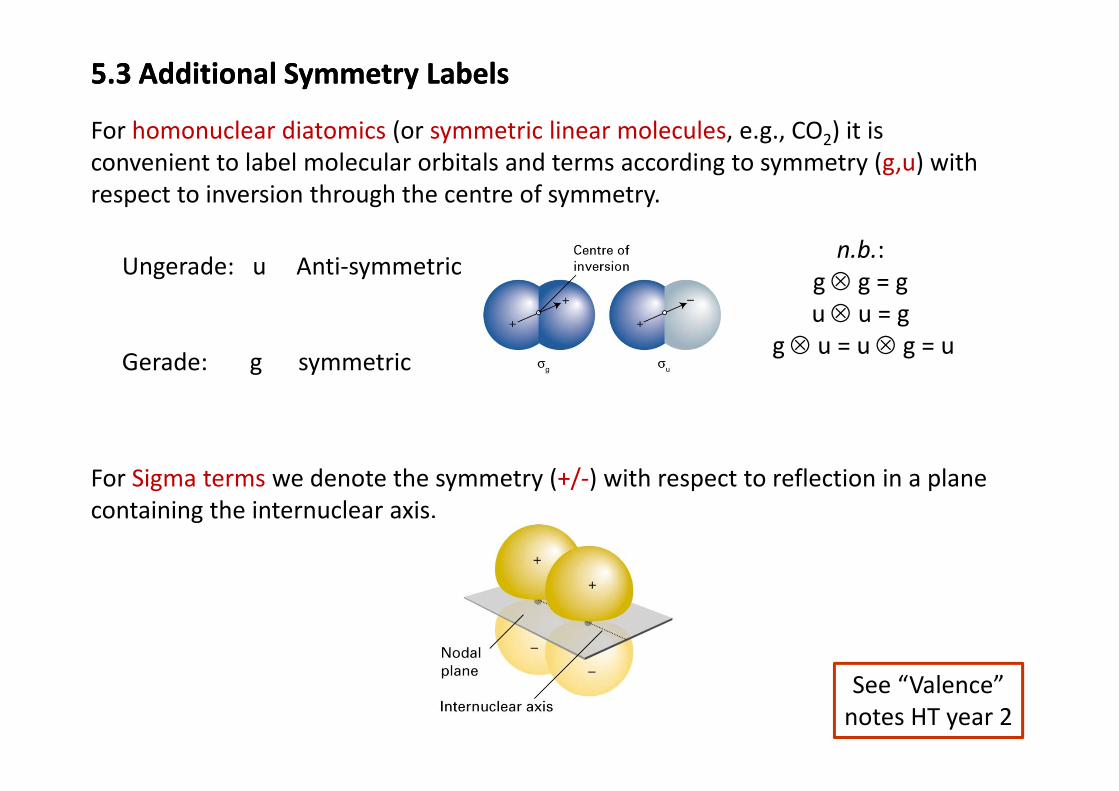
5.3 Additional Symmetry Labels5.3 Additional Symmetry Labels

For homonuclear diatomics (or symmetric linear molecules e g CO ) it isFor homonuclear diatomics (or symmetric linear molecules, e.g., CO2) it is convenient to label molecular orbitals and terms according to symmetry (g,u) with respect to inversion through the centre of symmetry.

Ungerade:   u     Anti‐symmetricn.b.:

g ⊗ g = g ⊗

Gerade:       g      symmetric

u ⊗ u = gg ⊗ u = u ⊗ g = u

For Sigma terms we denote the symmetry (+/‐) with respect to reflection in a planeFor Sigma terms we denote the symmetry ( / ) with respect to reflection in a plane containing the internuclear axis. 

See “Valence” notes HT year 2

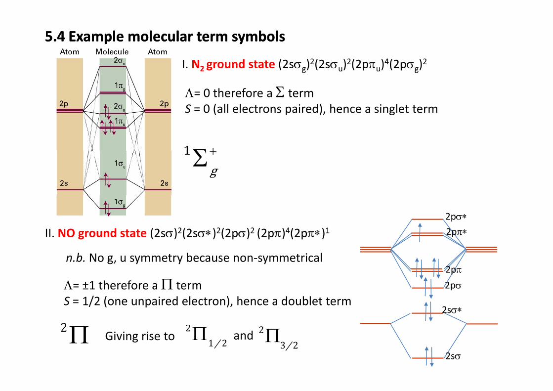
5.4 Example molecular term symbols5.4 Example molecular term symbols

I N ground state (2sσ )2(2sσ )2(2pπ )4(2pσ )2I. N2 ground state (2sσg)2(2sσu)2(2pπu)4(2pσg)2

Λ= 0 therefore a Σ termS 0 (all electrons paired) hence a singlet termS = 0 (all electrons paired), hence a singlet term

1 +Σ1 g+Σ

II. NO ground state (2sσ)2(2sσ∗)2(2pσ)2 (2pπ)4(2pπ∗)1 2pπ∗2pσ∗

n.b. No g, u symmetry because non‐symmetrical

2pσ2pπ

Λ= ±1 therefore a Π term

2sσ∗

2pσΛ= ±1 therefore a Π termS = 1/2 (one unpaired electron), hence a doublet term

2Π 2Π 2

2sσ

2Π Giving rise to 2

1 2/Π 23 2/Πand 

5.5 Example molecular term symbols5.5 Example molecular term symbols

III. O2 ground state (2sσg)2(2sσu)2(2pσg)2(2pπu)4(2pπg)2

Λ= 0, or ±2 therefore Σ, Δ terms ariseS = 0, or 1 singlets and triplets g ⊗ g = g all terms gerade

1 1 3 3 1 3g g g g g g+ − + −Σ Σ Σ Σ Δ Δ∴expect

But this neglects the Pauli Principle. 

In singlet states ψ i is antisymmetric Hence these can only be paired with symmetricIn singlet states, ψspin is antisymmetric. Hence these can only be paired with symmetric ψspace , i.e.,  g, + states. Likewise triplet states must be paired with g, – states. 

1 3 3− +Σ Σ Δ all violate Pauli and thus do not existg g gΣ Σ Δ all violate Pauli and thus do not exist

1 3 1+ −Σ Σ Δ Do exist, of which the triplet state is the lowest in energy g g gΣ Σ Δ p gy

(spin correlation)

Again, this is only a consideration for multiply occupied (but not full) orbitals

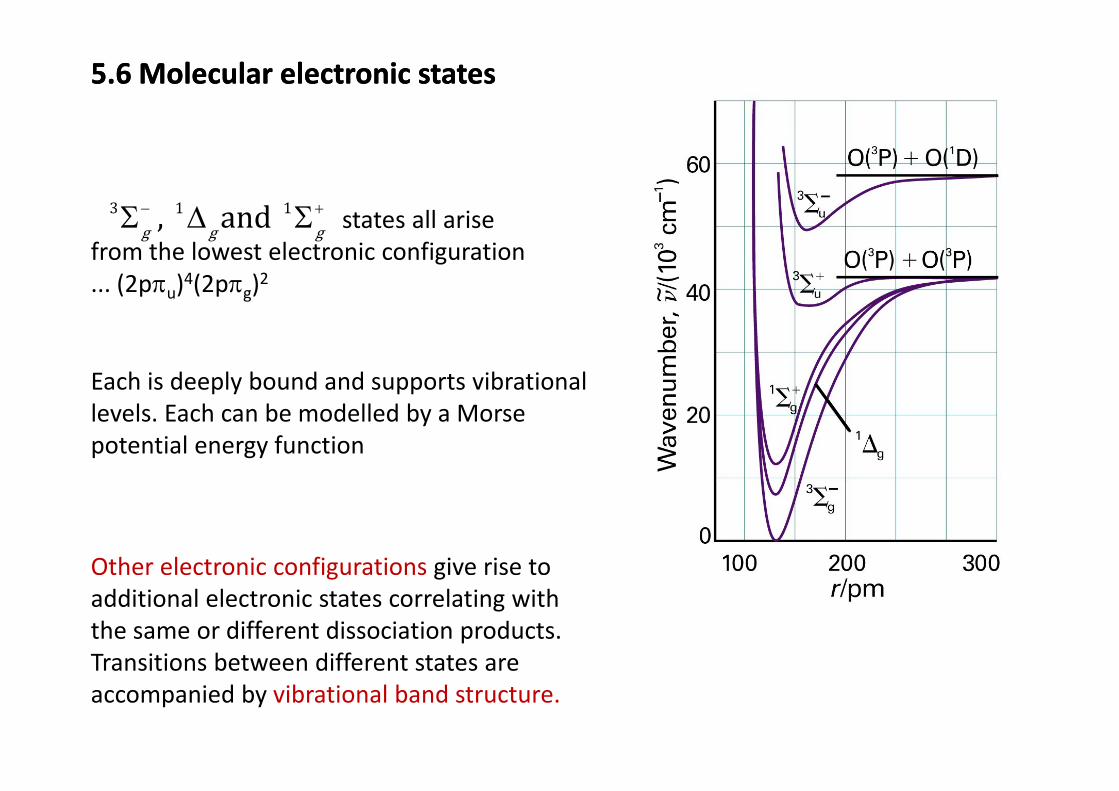
5.6 Molecular electronic states5.6 Molecular electronic states

3 1 1and− +Σ Δ Σ states all arise,  and g g gΣ Δ Σ states all arise from the lowest electronic configuration ... (2pπu)4(2pπg)2

Each is deeply bound and supports vibrationallevels. Each can be modelled by a Morse potential energy function

Other electronic configurations give rise to g gadditional electronic states correlating with the same or different dissociation products. Transitions between different states areTransitions between different states are accompanied by vibrational band structure.

5.7 Electronic Spectroscopy5.7 Electronic Spectroscopy

C id ld f i d th T iti Di l M t * ˆ ˆR d ⟨ ⟩∫Consider our old friend the Transition Dipole Moment 21 2 1 2 1R dψ μψ τ ψ μ ψ= = ⟨ ⟩∫Within the B O approximation Ψ = ψ (r)ψ (R) i i

ˆˆ q rμ =∑Within the B‐O approximation, Ψtot= ψel(r)ψvib(R) i∑

( ) ( ) ( ) ( )21 d  del vib el vib el vib el vibˆR e r R r r R r Rψ ψ μ ψ ψ ψ ψ ψ ψ∗ ∗′ ′ ′′ ′′ ′ ′ ′′ ′′= ⟨ ⟩ = − ∫∫ ( ) ( ) ( ) ( )∫∫

( ) ( ) ( ) ( )21 d del el vib vibR e r r r r R R Rψ ψ ψ ψ∗ ∗′ ′′ ′ ′′= − ∫ ∫Electronic 

transition momentVibrationaloverlap

Transition intensity ∝ ( ) ( )( ) ( ) ( )( )2 2221 d del el vib vibR r r r r R R Rψ ψ ψ ψ∗ ∗′ ′′ ′ ′′∝ ∫ ∫( ) ( )

Franck‐Condon factor(square of the vibrational

ΔΛ = 0, ±1ΔS = 0 and ΔΣ = 0

overlap integral)g ↔ u (where g, u exist)+ ↔ + ;  – ↔ – (for Σ−Σ transitions)

5.8 The Franck‐Condon Principle5.8 The Franck‐Condon Principle

Assumption: electronic transitions take place on such a short timescale that theAssumption: electronic transitions take place on such a short timescale that the nuclei remain frozen (R unchanged) during the transition.

We talk of “vertical transitions” between potential energy curves.

There is no selection rule governing the allowed vibrational changes accompanying an electronic transition.

Instead, the probability of undertaking a v” → v’ transition is governed by Franck‐Condon factors (the g y (overlap of the two vibrational wavefunctions).

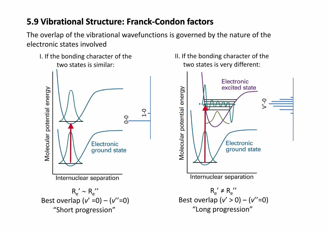
5.9 Vibrational Structure: Franck‐Condon factors5.9 Vibrational Structure: Franck‐Condon factorsThe overlap of the vibrational wavefunctions is governed by the nature of the

I. If the bonding character of the t t t i i il

II. If the bonding character of the two states is very different

The overlap of the vibrational wavefunctions is governed by the nature of the electronic states involved

two states is similar: two states is very different:

0 1‐0 V

’‐0

0‐0 1

Re’ ∼ Re’’ Re’ ≠ Re’’e eBest overlap (v’ =0) – (v’’=0)

“Short progression” Best overlap (v’ > 0) – (v’’=0)

“Long progression” 

5.10 Determining dissociation energies5.10 Determining dissociation energies

In some cases, Franck‐Condon overlap extends above the dissociation limit and excited‐state dissociation energies are measured directlyenergies are measured directly.

When this is not the case but several vibrational levels are excited it is possible to extrapolate to find theare  excited it is possible to extrapolate to find the dissociation limit.

2Recall, Morse oscillator: 21 12 2

0 1 2 3 ma

v e

x

e eGv

v v xv , , , ,

ω ω= + − += …

( )122ve e e

dG x vdv

ω ω= − + Which, at the dissociation limit (v+½)max becomes zero( )dv

( )10 2vdG x vω ω= = − +1ev ω

= −2eG D ω

= =( )20 2e e e maxx vdv

ω ω +2 2max

e e

vxω 4maxv e

e exω

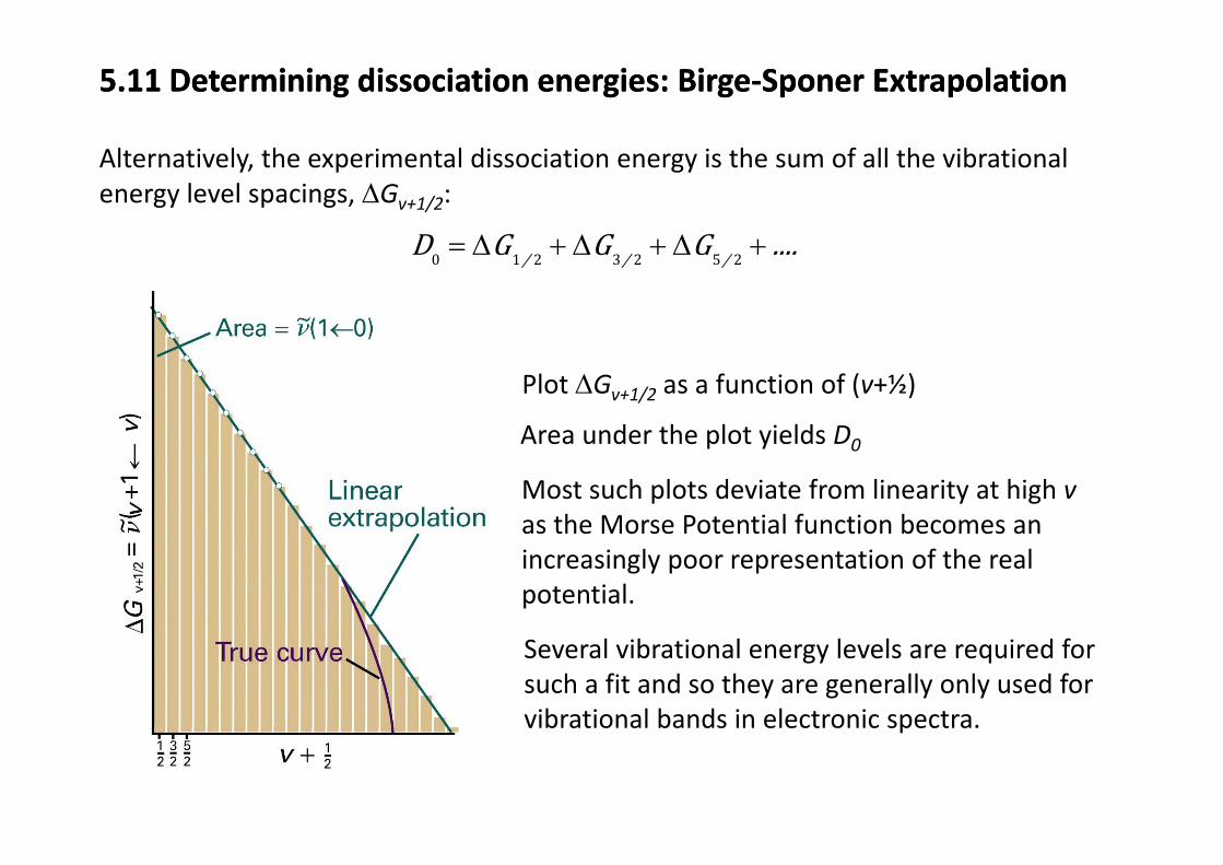
5.11 Determining dissociation energies: Birge‐Sponer Extrapolation5.11 Determining dissociation energies: Birge‐Sponer Extrapolation

Alternatively, the experimental dissociation energy is the sum of all the vibrationalenergy level spacings, ΔGv+1/2:

D G G GΔ Δ Δ0 1 2 3 2 5 2/ / /D G G G ....= Δ + Δ + Δ +

Area under the plot yields D

Plot ΔGv+1/2 as a function of (v+½)

Area under the plot yields D0

Most such plots deviate from linearity at high vas the Morse Potential function becomes anas the Morse Potential function becomes an increasingly poor representation of the real potential. 

Several vibrational energy levels are required for such a fit and so they are generally only used for vibrational bands in electronic spectra.vibrational bands in electronic spectra.

5.12 Rotational Structure in Electronic Spectra5.12 Rotational Structure in Electronic Spectra

e v

E T G Fhc

= + + JTotal term values:

Transition wavenumbers:  ( ) ( ) ( )e e v vT T G G F Fν ′ ′′ ′ ′′ ′ ′′= − + − + −J J

Electronic Vibrational RotationalElectronicTransition 

Vibrationaltransition

FCF

Rotationaltransition(ΔJ rules)

Example:   1Σ ‐1Σ ΔJ = ± 1, leads to P(J) and R(J) branches as in vib‐rot spectra [See section 4.7][ ]

However, much larger changes in rotational constants, of both sign, are now possible – band heads are commonly observed in electronic spectra, and may occur in either branch.

5.13 Band Heads in Electronic Spectra5.13 Band Heads in Electronic Spectra

( ) ( )( ) ( )( )2( ) ( )( ) ( )( )21 1el vibR B B B Bν−

′ ′′ ′ ′′= + + + + − +J J J

( ) ( ) ( ) 2el vibP B B B Bν

−′ ′′ ′ ′′= − + + −J J J

(1)

(2)( ) ( ) ( )el vib

In  vibration‐rotation spectra, B generally decreases slightly with v leading to bunching of lines in the R branch. In electronic transitions, the  change in <R2> can be large depending on the bonding character of the two orbitals between which the electron moves.

Band heads occur when lines in a branch coalesce, i.e.,   0dd

ν=

J

( )B B′ ′′In the R branch:  ( ) ( )( )2 1d B B B B

dν ′ ′′ ′ ′′= + + − +JJ ( ) ( )

( )1

2head

B BB B

′ ′′+= −

′ ′′−J

In the P branch:  ( ) ( )2d B B B Bd

ν ′ ′′ ′ ′′= − + + −JJ

( )( )2head

B BB B

′ ′′+=

′ ′′J( ) ( )d J ( )2 B B−

5.13 Band Heads in Electronic Spectra5.13 Band Heads in Electronic Spectra

Large change in Re in transition with result that B’<<B” –with result that B <<B  –rotational levels more closely spaced in upper state.

Bandhead in the R‐branch: 

increased spacing in P‐branch

CuH 1Σ ‐1Σ transition

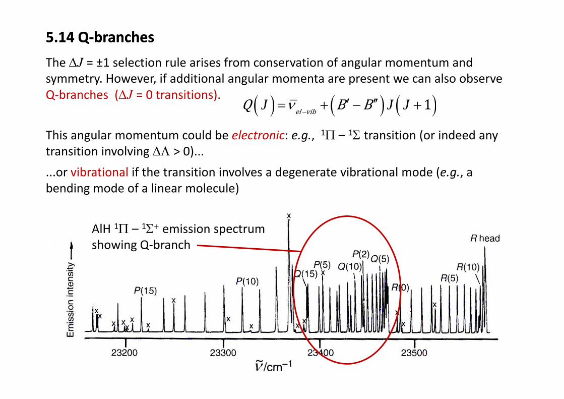
5.14 Q‐branches5.14 Q‐branches

The ΔJ = ±1 selection rule arises from conservation of angular momentum andThe ΔJ = ±1 selection rule arises from conservation of angular momentum and symmetry. However, if additional angular momenta are present we can also observe Q‐branches  (ΔJ = 0 transitions).  ( ) ( ) ( )1l bQ B Bν ′ ′′= + − +J J J

This angular momentum could be electronic: e.g.,  1Π – 1Σ transition (or indeed any transition involving ΔΛ > 0)...

( ) ( ) ( )1el vibQ B Bν−

+ +J J J

transition involving ΔΛ > 0)...

...or vibrational if the transition involves a degenerate vibrational mode (e.g., a bending mode of a linear molecule)

AlH 1Π – 1Σ+ emission spectrum showing Q branchshowing Q‐branch 

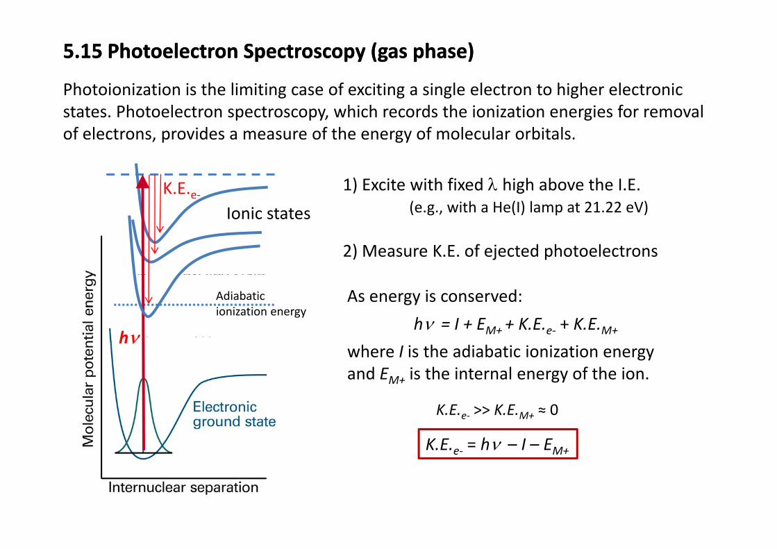
5.15 Photoelectron Spectroscopy (gas phase)5.15 Photoelectron Spectroscopy (gas phase)

Photoionization is the limiting case of exciting a single electron to higher electronicPhotoionization is the limiting case of exciting a single electron to higher electronic states. Photoelectron spectroscopy, which records the ionization energies for removal of electrons, provides a measure of the energy of molecular orbitals.

Ionic statesK.E.e‐ 1) Excite with fixed λ high above the I.E.

(e.g., with a He(I) lamp at 21.22 eV)Ionic states (e.g., with a He(I) lamp at 21.22 eV)

2) Measure K.E. of ejected photoelectrons

Adiabatic ionization energy

As energy is conserved: 

hν = I + EM+ + K.E.e‐ + K.E.M+hνwhere I is the adiabatic ionization energy and EM+ is the internal energy of the ion.

hν

K.E.e‐ >> K.E.M+ ≈ 0

K.E.e‐ = hν – I – EM+

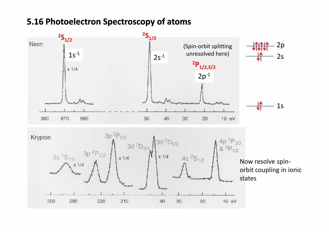
5.16 Photoelectron Spectroscopy of atoms5.16 Photoelectron Spectroscopy of atoms2S1/22S

2s‐11s‐12P

S1/22S1/2(Spin‐orbit splitting unresolved here) 2s

2p

2p‐1

2P1/2,3/2

1s

Now resolve spin‐bit li i i iorbit coupling in ionic 

states

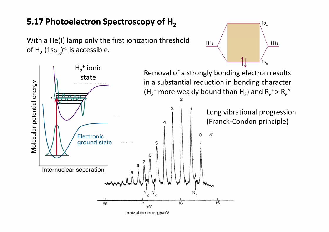
5.17 Photoelectron Spectroscopy of H25.17 Photoelectron Spectroscopy of H2

With a He(I) lamp only the first ionization threshold of H2 (1sσg)‐1 is accessible.

Removal of a strongly bonding electron results in a substantial reduction in bonding character(H + kl b d th H ) d R + R ”

H2+ ionic state

(H2+ more weakly bound than H2) and Re+ > Re”

Long vibrational progression(Franck‐Condon principle)

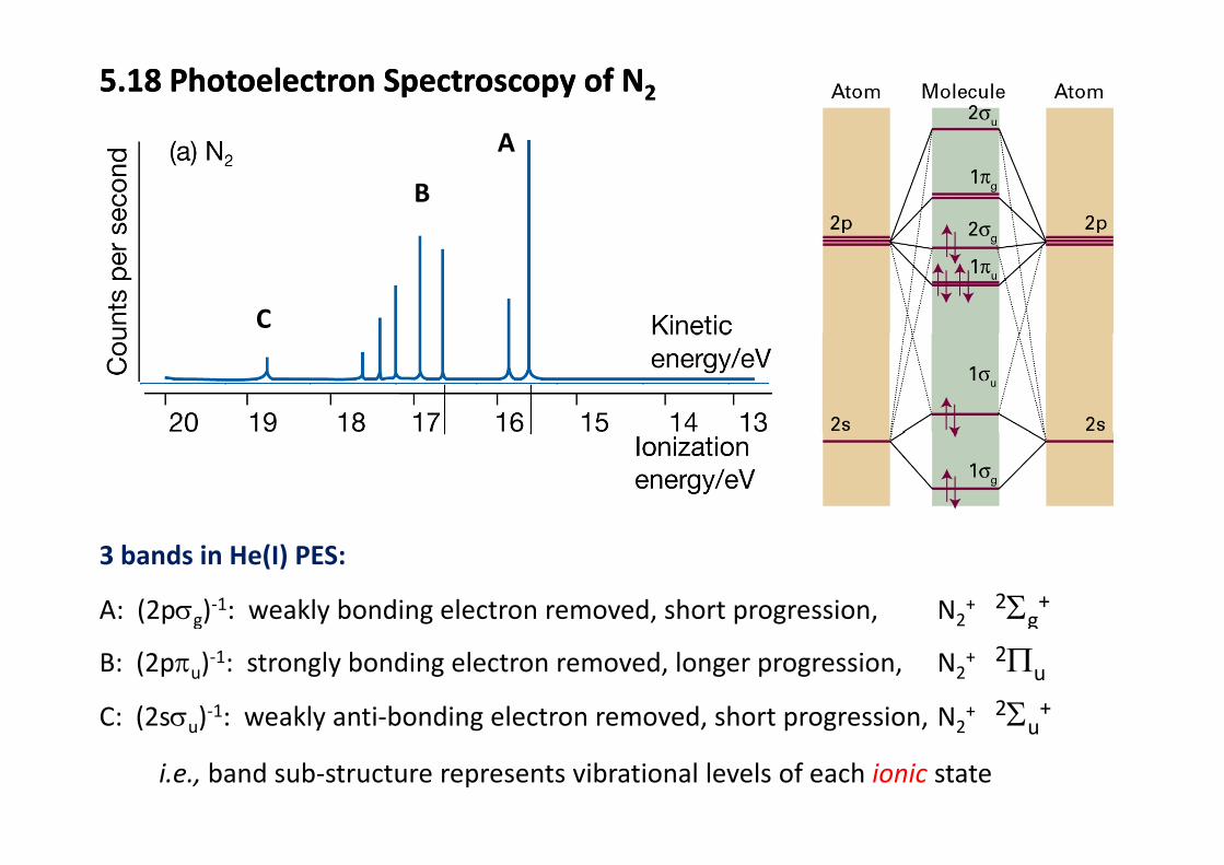
5.18 Photoelectron Spectroscopy of N25.18 Photoelectron Spectroscopy of N2

AA

B

C

3 bands in He(I) PES:

A:  (2pσg)‐1:  weakly bonding electron removed, short progression,  N2+ 2Σg

+

B:  (2pπu)‐1:  strongly bonding electron removed, longer progression,  N2+ 2Πu

C:  (2sσu)‐1:  weakly anti‐bonding electron removed, short progression, N2+ 2Σu

+( u) y g , p g , 2 u

i.e., band sub‐structure represents vibrational levels of each ionic state