selected quantitative methods - harry ganzeboom lecture3.pdf · selected quantitative methods...

SQM 3: Binomial Logistic RegressionReview of Quantitative

Methods

1

Selected Quantitative MethodsLecture 3

(Binomial) Logistic Regression

Harry B.G. Ganzeboom

VU-FSW Master Social Research

September 14-16 2011


Methods

2SQM 3: Review of Quantitative Methods

2

Wanneer gebruik je logistische regressie?

• OLS regressie� afhankelijke variabele op interval/ratio niveau

• Logistische regressie wordt gebruikt wanneer de afhankelijke variabele dichotoom is (0-1)

• Voorspellen van de kans P op een bepaalde gebeurtenis via een kansverhouding [odds] en een logit [log odds].

• Verder: veel hetzelfde als bij OLS regressie


Methods

3Review of Quantitative Methods 3

Logistic regression

• We start by studying binomial logistic regression, which relates a binary (0,1) Y-variable to a linear (additive) specification of the X-variables.

• The changes relative to OLS regression are all in the Y-part:– The model is linear in logits.– The estimation procedure is entirely different. In particular it is

iterative.

– Variance, sum-of-squares and fit statistics are entirely different from OLS regression.

– Direct and indirect effects are also complicated.


Methods


Various forms

• The binomial logistic regression is not only frequently used in research practice (any variable can be dichotomized!), but it is also a necessary first step to other, more complicated (and sometimes more informative and more powerful) models for discrete Y-variables.– Multinomial logistic regression (Y has more than 2 categories).– Ordered logistic regression (Y has more than 2 categories which

can be ordered). This model is often used for education as an outcome.

– Conditional logistic regression (Y has (many) more than 2 categories, which can be scaled on multiple dimensions. This model is very interesting for e.g. political party choice, occupational choice.


Methods


Het lineaire probabiliteitsmodel

• Het is goed mogelijk omde kans P op een bepaalde gebeurtenis te voorspellen met gewone (OLS) regressie:het ‘lineaire probabiliteitsmodel’.

• Dit stuit wel op een aantal problemen:– Het kan leiden tot onmogelijke verwachte waarden (< 0 of > 1.0).– Dichotome afhankelijke variabelen leiden noodzakelijk tot

heteroskedasticiteit, namelijk geringe residuele variantie bij deextremen van de regressielijn.

– Mede om deze reden kloppen de inferentieel statistische conclusies(standard errors, significantie) niet.

• Dit is allemaal ernstig bij zeer scheef verdeelde afhankelijke variabelen (gemiddelde / verwachte P dichtbij1 of 0).


Methods


More on OLS for binary Y

• These often stated reasons to do logistic analysis are in practice not so relevant.– Negative expected values are in practice rare, and even if so: so

what?– OLS significance tests are in practice very close to their logistic

counterparts.

• Do not tell anybody, but I recommend strongly to run an OLS on your problem before you start doing logistic.

• There is a much better reason to prefer logistic over OLS: logistic regression coefficients are insensitive to marginal distributions. This is very important in practical problems of comparative research (between countries, between periods).


Methods


Kansen, kansverhouding, logit –1

• Afhankelijke variabele is kans op een gebeurtenis.

• Kans op categorie 1 is P; kans op categorie 0 is 1-P

• Kansverhouding (Odds) is P/(1-P).• Logit: ln(P/(1-P).


Methods


Logaritmes- 1

• Logaritme X: tot welke macht moet je een grondtal verheffen om Xte verkrijgen. Zie bv.: http://nl.wikipedia.org/wiki/Logaritme.

• Grondtal 10: 10log(100)=2

• Grondtal 2: 2log(64) = 6.

• Grondtal e = exp = 2.718:elog(100) = ln(100) = 4.61.

• Ln(a*b) = ln(a)+ln(b)

• exp(a+b) = exp(a)*exp(b)

• Ln(exp(a+b)) = a+b

• Vermenigvuldigen� optellen

• Delen� Aftrekken

• Machtverheffen� vermenigvuldigen of delen


Methods


Logaritmes- 2

• Ln (2.718) = 1

• Ln (2) = .69

• Ln (1) = 0

• Ln (.5) = -.69

• Ln (0) = infinity = undefined

• Exp(1) = 2.718

• Exp(0) = 1


Methods


P versus odds


Methods


P odds logit

0.90 9.00 2.20

0.80 4.00 1.39

0.70 2.33 0.85

0.60 1.50 0.41

0.50 1.00 0.00

0.40 0.67 -0.41

0.30 0.43 -0.85

0.20 0.25 -1.39

0.10 0.11 -2.20

0.09 0.10 -2.31

0.08 0.09 -2.44

0.07 0.08 -2.59

0.06 0.06 -2.75

0.05 0.05 -2.94

0.05 0.05 -2.94

0.04 0.04 -3.18

0.03 0.03 -3.48

0.02 0.02 -3.89

0.01 0.01 -4.60


Methods

12

P versus Odds

• Note that for P < .10, P is very close to the odds.– P = .05 � odds = .05/.95 = .052

– P = .10 � odds = .10/.90 = .111

• But:– P = .50 � odds = .50/.50 = 1.00

� For small effects, the exponentiated coeffients give the same effects on odd and on P.


Methods


P versus logit (ln transformatie)


Methods


Logit versus P


Methods


Kans, kansverhoudingen logits - 2

• Logit is de natuurlijke logaritme (ln) van de odds: logit= ln(P/(1-P))

• DUS:• Omzetten van logits naar odds: exp(logit) � odds • Omzetten van odds naar logits:ln(odds)� logit• Omzetten van logit /odds naar P:

P = 1 / (1+exp(-logit))P = odds / (1+odds)

These transformations are available in SPSS as ‘predicted value’.


Methods


Odds and odds-ratio’s

• Many, many people confuse odds and odds-ratio.

• Odds is a ratio of two (complementary) probabilities.

• Odds-ratio is a ratio of two odds.• Odds is a attribute of one variable.• Odds-ratio is a relationship between two

variables.


Methods


Invariance of odds-ratio’s

• Odds ratio’s are insensitive to marginal weights.

• This is of immense importance in “case-control” studies

• As well as in comparative studies of changes / differences, e.g. voting, occupation, and many other things.


Methods


Invariance of odds-ratio’s

100 50 0.50 4.00

50 100 2.00

1000 500 0.50 4.00

50 100 2.00

100 500 5.00 4.00

50 1000 20.00


Methods


Studerendin ISSP 2006 (1)

• Voorbeeld: studerend in ISSP2006. Data voor leeftijd18-64, N=1575. Gemiddelde is 3.2%, oftewel .032.

• Student zijn is zeer sterk gedifferentieerd naar leeftijd.Het komt eigenlijk alleen bij jonge mensen voor.

• OLS Model: STUDENT = 0.239 - .0047 * AGECAT.• De slope is zeer significant: t = 12.8.• Data worden zeer slecht gerepresenteerd door het

lineaire probabiliteitsmodel; verwachte kans op student zijn voor ouderen wordt negatief (-4%).


Methods


Studentenin ISSP 2006 - 2

• Logistisch model:– Logit(STUDENT) = 5.310 – 0.269 * AGECAT.

• Geëxponentieerd:– Odds(STUDENT) = exp(5.310 – 0.269 * AGECAT).

– Odds(STUDENT) = exp(5.310)*exp(-.269*AGECAT)

• In kansen:– STUDENT = 1/(1+exp(-logit))

• LET OP: T-waarde = 9.3 (anders/kleiner dan bijOLS!)


Methods


Studentenin ISSP 2006 - 3

ObservedAGE N Data OLS LOGIST ODDS LOGIT

19 22 0.682 0.150 0.549 1.219 0.19822 54 0.389 0.136 0.352 0.544 -0.60930 283 0.032 0.099 0.059 0.063 -2.76240 460 0.007 0.052 0.004 0.004 -5.45350 385 0.005 0.006 0.000 0.000 -8.14360 371 0.000 -0.041 0.000 0.000 -10.834

verwachte waarden


Methods


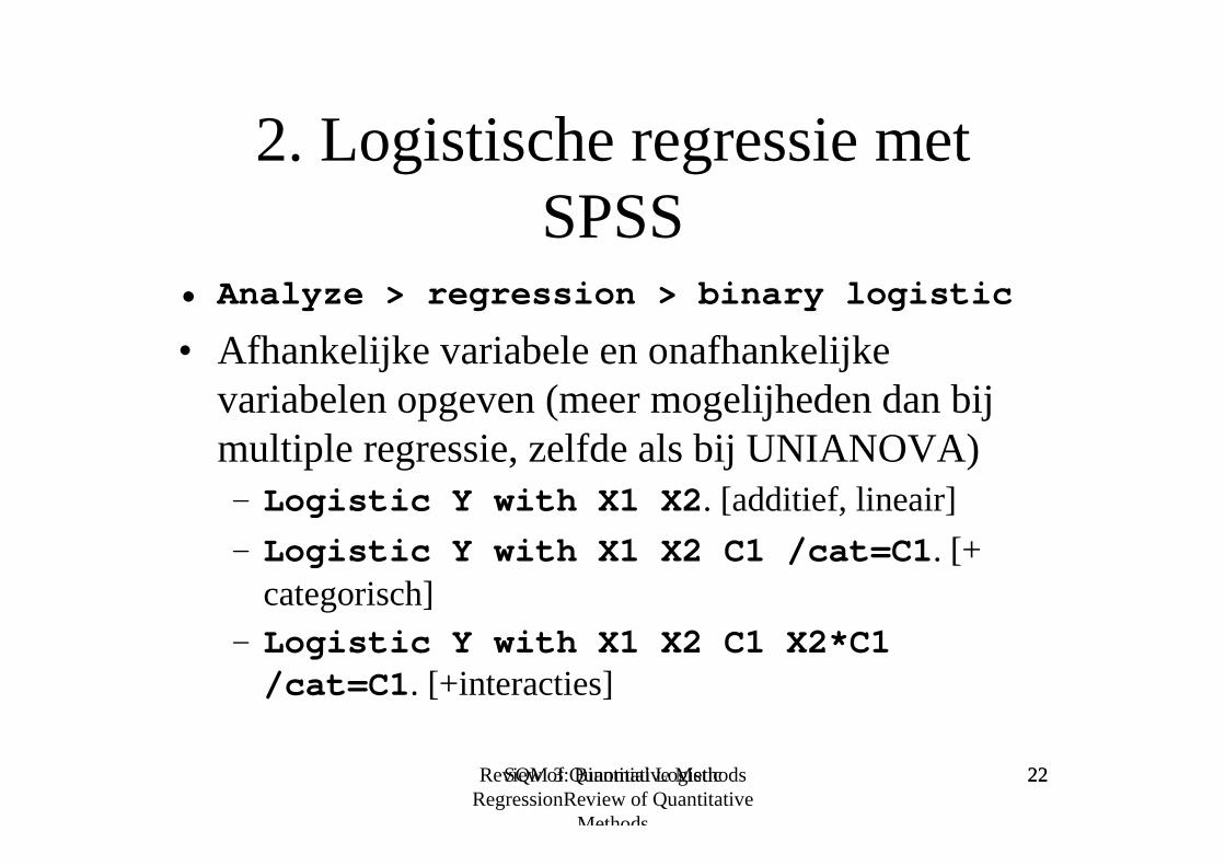
2. Logistische regressie met SPSS

• Analyze > regression > binary logistic

• Afhankelijke variabele en onafhankelijke variabelen opgeven (meer mogelijheden dan bijmultiple regressie, zelfde als bij UNIANOVA)– Logistic Y with X1 X2. [additief, lineair]

– Logistic Y with X1 X2 C1 /cat=C1. [+categorisch]

– Logistic Y with X1 X2 C1 X2*C1 /cat=C1. [+interacties]


Methods


Tabel ‘Case Processing Summary’

Case Processing Summary

1575 100.0

0 .0

1575 100.0

0 .0

1575 100.0

Unweighted Cases a

Included in Analysis

Missing Cases

Total

Selected Cases

Unselected Cases

Total

N Percent

If weight is in effect, see classification table for the totalnumber of cases.

a.


Methods


Tabel ‘Dependent Variable Encoding’

Dependent Variable Encoding

0

1

Original Value

0

1

Internal Value


Methods


Tabel ‘Omnibus Tests of Model coefficients’

Omnibus Tests of Model Coefficients

187.933 1 .000

187.933 1 .000

187.933 1 .000

Step

Block

Model

Step 1

Chi-square df Sig.


Methods


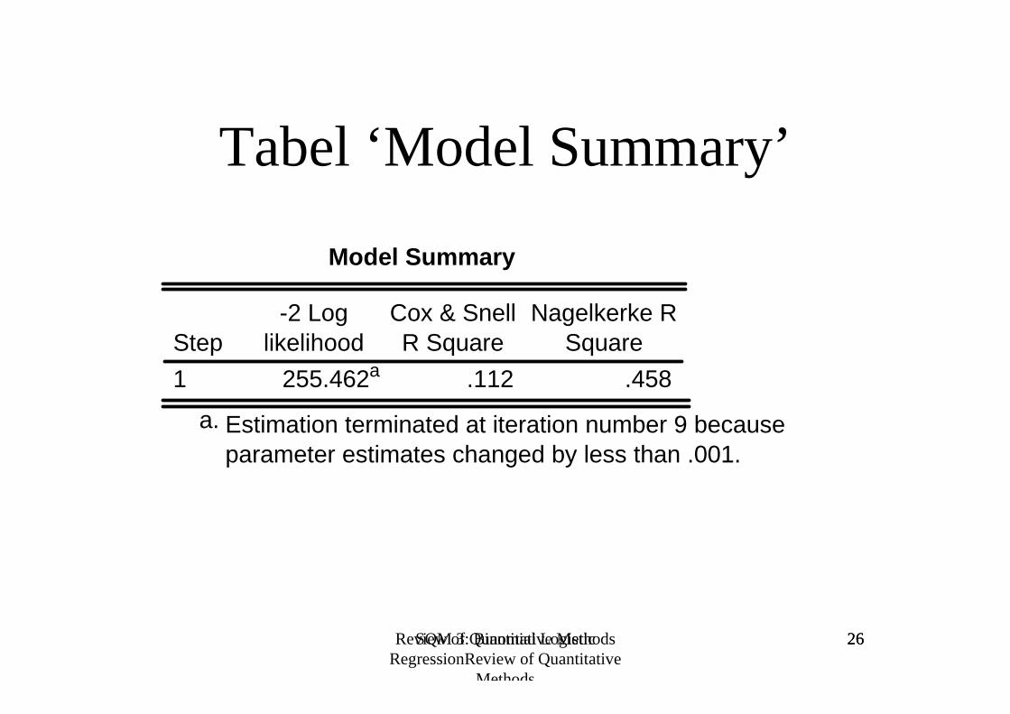
Tabel ‘Model Summary’

Model Summary

255.462a .112 .458

Step

1

-2 Loglikelihood

Cox & SnellR Square

Nagelkerke RSquare

Estimation terminated at iteration number 9 becauseparameter estimates changed by less than .001.

a.


Methods


Tabel ‘Classification Table’

Classification Tablea

1518 7 99.5

35 15 30.0

97.3

Observed

0

1

unempl

Overall Percentage

Step 1

0 1

unempl PercentageCorrect

Predicted

The cut value is .500a.


Methods


Een paar handigheden

• Codeer je afhankelijke variabele altijd zelf 0/1.

• Bekijk missing values voordat je begint. Logistic kan nietsmet ‘pairwise’. Evt. dus substitutie toepassen.

• Net zoals bij OLS regressie, is interpretatie eenvoudiger als je X variabelen een 0 bevatten en een gemakkelijke eenheid hebben.

• Afzonderlijke coefficienten kun je op significantie toetsenmet t = b/SE.

• Na enige oefening zijn de exp(B) coefficienten gemakkelijker te interpreteren dan de logistische.


Methods


Table ‘Variables in the Equation’:

Variables in the Equation

-.269 .029 84.845 1 .000 .764

5.310 .783 46.034 1 .000 202.396

agecat

Constant

Step 1aB S.E. Wald df Sig. Exp(B)

Variable(s) entered on step 1: agecat.a.


Methods


Logistische en multiplicatieve regressiecoëfficiënten

• B geeft de verandering in de logit (=log odds) van de afhankelijke variabele aan bij één eenheid verandering van X. Het model is lineair in de logits.

• Exp(B) is de multiplicatieve verandering in de odds met een eenheid verandering van X ten opzichte van odds baseline (=multiplicatieve intercept).– Exp(B) < 1: afname van odds

– Exp(B) > 1: toename van odds

• Bij categorische variabelen kunnen we exp(B) interpreteren als eenodds-ratio [OR] = verhouding tussen twee odds.

• In continuous variables exp(B) denote how much the odds change (multiplicatively), if we move 1 unit of X.


Methods


Multiplicatieve coefficientenen de odds-ratio OR

• Odds = exp (B0 + B1*X1)

• Odds = exp(B0)*exp(B1*X1)

• Als X= 0: odds = exp(B0)*exp(0) = exp(B0)

• Als X=1: odds = exp(B0)*exp(B1)

• Odds Ratio OR: exp(B0)*exp(B1) / exp(B0) = exp(B1)


Methods


Geen gestandaardiseerdeB’s

• Anders dan bij OLS heeft logistic geen gestandaardiseerde coefficienten.

• B’s zijn daarom alleen met elkaar vergelijkbaar als hun eenheden vergelijkbaar zijn.

• Wil je toch gestandaardiseerde coefficienten hebben, dan zul je eerst zelf de X-en moeten standaardiseren (=voorzien van vergelijkbare meeteenheid).


Methods


Inferentiele statistiek

• Logistic geeft niet de bij OLS gebruikelijke T-toets: t = B/SE. Deze kun je wel zelf berekenen.

• Wald statistic is t2. Vergelijk met Chi2 of F-tabelmet 1, veel vrijheidsgraden. Kritieke waarde: 3.84.

• SE’s behoren horen bij logits. Betrouwbaarheids-intervalllen rondom logits zijn symmetrisch,rondom multiplicatieve coefficienten zijn ze asymmetrisch.


Methods


3. Logistische regressiemet nominale onafhankelijke variabelen

• Bij logistic behoef je niet zelf dummy-variabelen aan te maken by categorische X (het mag wel).

• ../cat=X1 /contrast(X1)=indicator(1)geeft aan dat X1 categorisch is en 1 de referentie-categorie is.

• De output kan behoorlijk verwarrend zijn. Letgoed op de “Categorical variable codings”.

• De Wald statistic is nu een test op gezamenlijke bijdrage van de dummy-variabelen.


Methods


Tabel ‘Categorical variablecodings’

Categorical Variables Codings

22 .000 .000 .000 .000 .000

53 1.000 .000 .000 .000 .000

276 .000 1.000 .000 .000 .000

453 .000 .000 1.000 .000 .000

379 .000 .000 .000 1.000 .000

363 .000 .000 .000 .000 1.000

19

22

30

40

50

60

agecat

Frequency (1) (2) (3) (4) (5)

Parameter coding


Methods


4. Rapporteren van een logistische regressie

• Resultaten van de logistische regressie zowel weergeven – in een tabel

– als in de tekst

• In de tekst ook inhoudelijk interpreteren van de resultaten


Methods


Tabel x. Logistische regressieanalyse van kerklidmaatschap op leeftijd, sekse, opleiding, urbanisatiegraad en burgerlijke status (N=4059)

B S.E. Wald df P Exp(B)

Sekse

Leeftijd

Opleiding

Urbanisatiegraad

Burgerlijke staat

Ongehuwd

Gescheiden

Verweduwd


Methods

3838

Welke zaken in de tekst vermelden?

• Nagelkerke R2 = kwaliteit van het model / samenhang

• OR = Odds ratio’s (% verandering bij eenheidsverandering of verschil tussen twee categorieën)

• P-waarde = is het effect van de onafhankelijke variabele significant en op welk niveau (p <0,05; p<0,01; p<0,001)?

• Voorbeeld (OR=0,34 ; p<0,01)

selected quantitative methods - harry ganzeboom lecture3.pdf · selected quantitative methods...

Documents