sfb 609 - fachbereich mathematik · sfb 609 sonderforschungsbereich 609 elektromagnetische...
TRANSCRIPT
SFB 609
Sonderforschungsbereich 609Elektromagnetische Strömungsbeeinflussung inMetallurgie, Kristallzüchtung und Elektrochemie
M. Hinze, O. Pfeiffer
Active Closed Loop Control OfWeakly Conductive Fluids.
SFB-Preprint SFB609-20-2004 .
Preprint ReiheSFB 609

Diese Arbeit ist mit Unterstützung des von der DeutschenForschungsgemeinschaft getragenen Sonderforschungsbereiches 609entstanden und als Manuskript vervielfältigt worden.
Dresden, Oktober 2004
The list of preprints of the Sonderforschungsbereich 609 is available at:http://www.tu-dresden.de/mwilr/sfb609/pub.html
ACTIVE CLOSED LOOP CONTROL OF WEAKLY CONDUCTIVE FLUIDS
M. HINZE, O. PFEIFFERTECHNISCHE UNIVERSITÄT DRESDEN
INSTITUT FÜR NUMERISCHE MATHEMATIKZELLESCHER WEG 12-14, 01069 DRESDEN
GERMANY
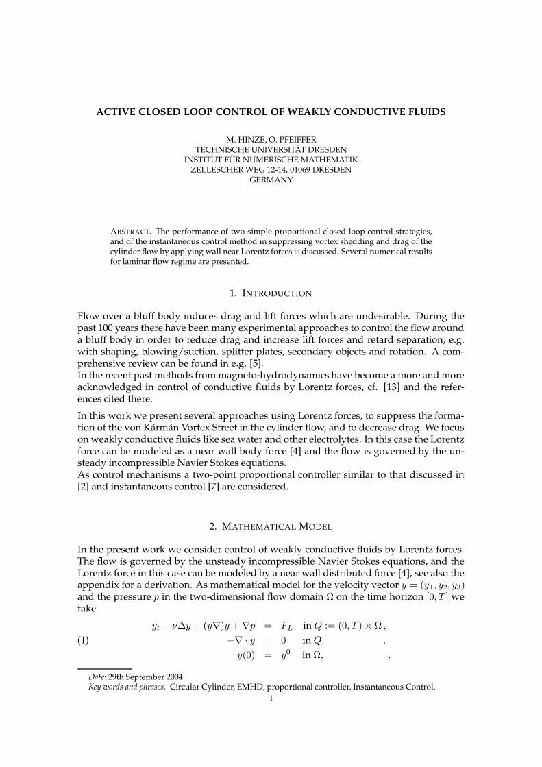
ABSTRACT. The performance of two simple proportional closed-loop control strategies,and of the instantaneous control method in suppressing vortex shedding and drag of thecylinder flow by applying wall near Lorentz forces is discussed. Several numerical resultsfor laminar flow regime are presented.
1. INTRODUCTION
Flow over a bluff body induces drag and lift forces which are undesirable. During thepast 100 years there have been many experimental approaches to control the flow arounda bluff body in order to reduce drag and increase lift forces and retard separation, e.g.with shaping, blowing/suction, splitter plates, secondary objects and rotation. A com-prehensive review can be found in e.g. [5].In the recent past methods from magneto-hydrodynamics have become a more and moreacknowledged in control of conductive fluids by Lorentz forces, cf. [13] and the refer-ences cited there.
In this work we present several approaches using Lorentz forces, to suppress the forma-tion of the von Kármán Vortex Street in the cylinder flow, and to decrease drag. We focuson weakly conductive fluids like sea water and other electrolytes. In this case the Lorentzforce can be modeled as a near wall body force [4] and the flow is governed by the un-steady incompressible Navier Stokes equations.As control mechanisms a two-point proportional controller similar to that discussed in[2] and instantaneous control [7] are considered.
2. MATHEMATICAL MODEL
In the present work we consider control of weakly conductive fluids by Lorentz forces.The flow is governed by the unsteady incompressible Navier Stokes equations, and theLorentz force in this case can be modeled by a near wall distributed force [4], see also theappendix for a derivation. As mathematical model for the velocity vector y = (y1, y2, y3)and the pressure p in the two-dimensional flow domain Ω on the time horizon [0, T ] wetake
yt − ν∆y + (y∇)y + ∇p = FL in Q := (0, T ) × Ω ,
−∇ · y = 0 in Q ,(1)y(0) = y0 in Ω, ,
Date: 29th September 2004.Key words and phrases. Circular Cylinder, EMHD, proportional controller, Instantaneous Control.
1
ACTIVE CLOSED LOOP CONTROL OF WEAKLY CONDUCTIVE FLUIDS 2
supplied with appropriate boundary conditions. Here the Lorentz force is given by
FL(x) = J0B0g(φ)e−πa·dist[x,cylindersurface]~t,
with
g(φ) =
1,−1,
0,
φ0 ≤ φ ≤ φ1
π + φ0 ≤ φ ≤ π + φ1
else,
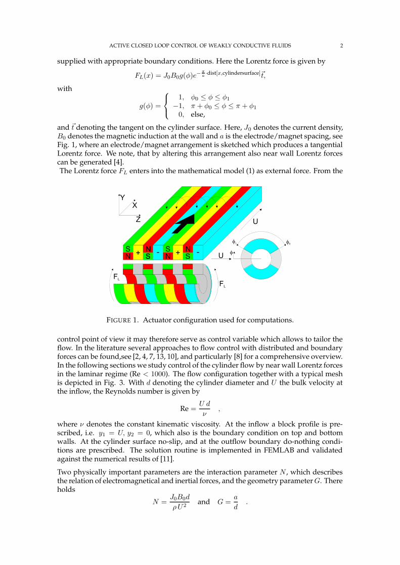
and ~t denoting the tangent on the cylinder surface. Here, J0 denotes the current density,B0 denotes the magnetic induction at the wall and a is the electrode/magnet spacing, seeFig. 1, where an electrode/magnet arrangement is sketched which produces a tangentialLorentz force. We note, that by altering this arrangement also near wall Lorentz forcescan be generated [4].The Lorentz force FL enters into the mathematical model (1) as external force. From the
FIGURE 1. Actuator configuration used for computations.
control point of view it may therefore serve as control variable which allows to tailor theflow. In the literature several approaches to flow control with distributed and boundaryforces can be found,see [2, 4, 7, 13, 10], and particularly [8] for a comprehensive overview.In the following sections we study control of the cylinder flow by near wall Lorentz forcesin the laminar regime (Re < 1000). The flow configuration together with a typical meshis depicted in Fig. 3. With d denoting the cylinder diameter and U the bulk velocity atthe inflow, the Reynolds number is given by
Re =U d
ν,
where ν denotes the constant kinematic viscosity. At the inflow a block profile is pre-scribed, i.e. y1 = U, y2 = 0, which also is the boundary condition on top and bottomwalls. At the cylinder surface no-slip, and at the outflow boundary do-nothing condi-tions are prescribed. The solution routine is implemented in FEMLAB and validatedagainst the numerical results of [11].
Two physically important parameters are the interaction parameter N , which describesthe relation of electromagnetical and inertial forces, and the geometry parameter G. Thereholds
N =J0B0d
ρU2and G =
a
d.
ACTIVE CLOSED LOOP CONTROL OF WEAKLY CONDUCTIVE FLUIDS 3
In order to compare calculations with different geometry parameters, the so-called scaledinteraction parameter N · G is used, compare [11].
The control target consists in reducing the drag force FD which is composed of the threedifferent parts, i.e.
FD = FDf+ FDp + FDem ,
with
FDf=
∫
∂cyl.ρν∂η(y·~t)·η2dS , FDp = −
∫
∂cyl.p η1·e2dS , FDem = −J0B0
a
πD(cos φ0−cos φ1) .
Here η = (η1, η2)t denotes the outward normal on the cylinder surface. The correspond-
ing drag coefficients are given by
CD =2FD
ρU2D, CDf
=2FDf
ρU2D, CDp =
2FDp
ρU2D, and CDem =
2FDem
ρU2D
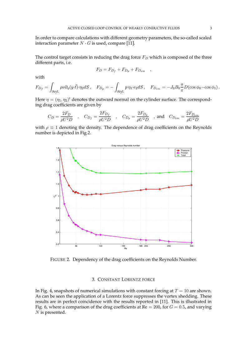
with ρ ≡ 1 denoting the density. The dependence of drag coefficients on the Reynoldsnumber is depicted in Fig.2.
46 100 150 188 200 250 3000.2
0.4
0.6
0.8
1
1.2
1.4
1.6
1.8
Re
Cd
i
Drag versus Reynolds number
PressureFrictionTotal
FIGURE 2. Dependency of the drag coefficients on the Reynolds Number.
3. CONSTANT LORENTZ FORCE
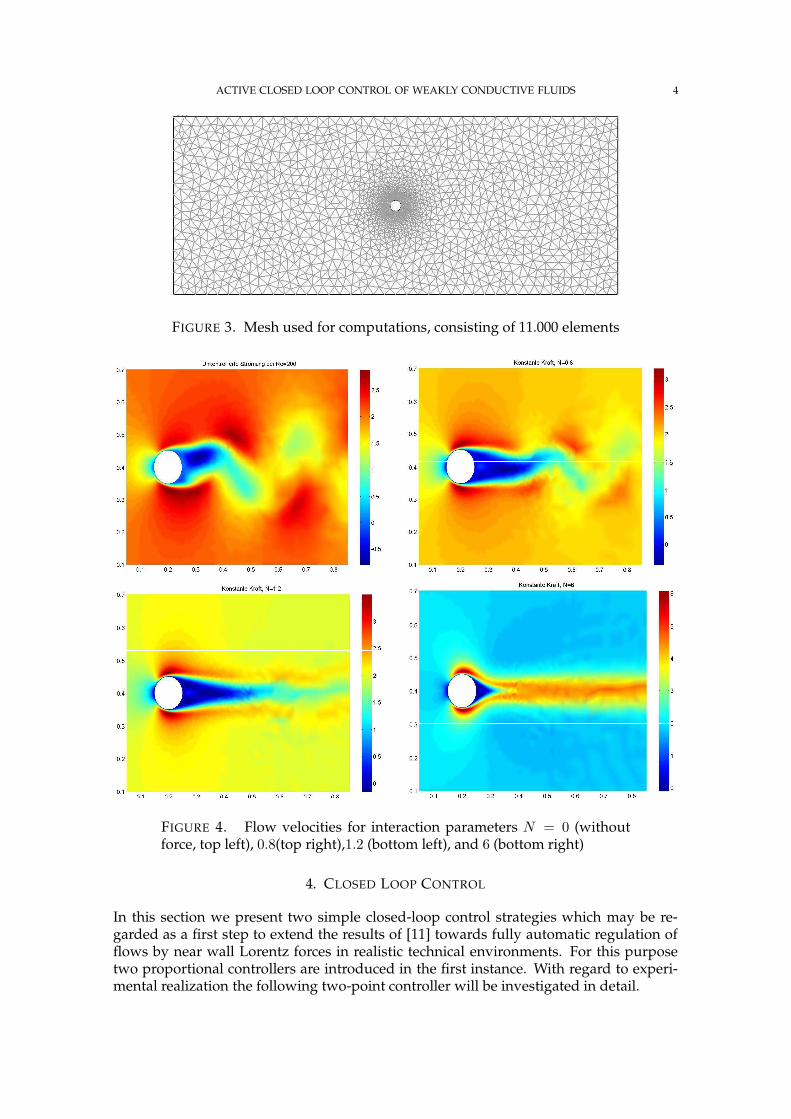
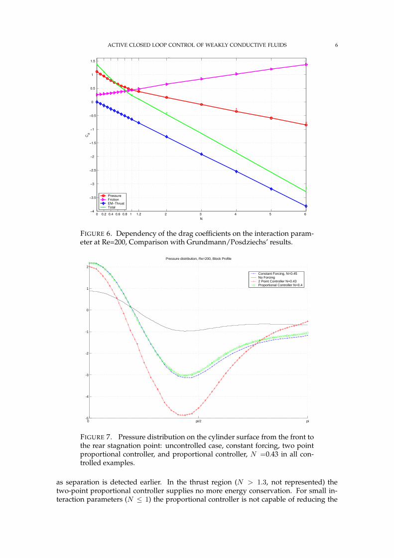
In Fig. 4, snapshots of numerical simulations with constant forcing at T = 10 are shown.As can be seen the application of a Lorentz force suppresses the vortex shedding. Theseresults are in perfect coincidence with the results reported in [11]. This is illustrated inFig. 6, where a comparison of the drag coefficients at Re = 200, for G = 0.5, and varyingN is presented.
ACTIVE CLOSED LOOP CONTROL OF WEAKLY CONDUCTIVE FLUIDS 4
FIGURE 3. Mesh used for computations, consisting of 11.000 elements
FIGURE 4. Flow velocities for interaction parameters N = 0 (withoutforce, top left), 0.8(top right),1.2 (bottom left), and 6 (bottom right)
4. CLOSED LOOP CONTROL
In this section we present two simple closed-loop control strategies which may be re-garded as a first step to extend the results of [11] towards fully automatic regulation offlows by near wall Lorentz forces in realistic technical environments. For this purposetwo proportional controllers are introduced in the first instance. With regard to experi-mental realization the following two-point controller will be investigated in detail.
ACTIVE CLOSED LOOP CONTROL OF WEAKLY CONDUCTIVE FLUIDS 5
0 0.5 1 1.5 2 2.5 3
-0.6
-0.4
-0.2
0
0.2
0.4
0.6
0.8
1
1.2
Zeit in Sekunden
Unkontrollierte offene Strömung, Re=200, N=0, Blockprofil
GesamtwiderstandDruckwiderstandReibungswiderstandAuftrieb
0 0.5 1 1.5 2 2.5 3
-0.4
-0.2
0
0.2
0.4
0.6
0.8
1
1.2
Constant Forcing, Re=200, N=0.43, Block Profile
Time in Seconds
Total DragPressure DragViscous DragLift
0 0.1 0.2 0.3 0.4 0.5 0.6 0.7 0.8 0.9
-0.5
0
0.5
1
1.5
Time in Seconds
Two-Point-Controller, Re=200, N=0.43, Block Profile
Total DragPressure DragViscous DragLift
0 0.5 1 1.5 2 2.5 3
-0.4
-0.2
0
0.2
0.4
0.6
0.8
1
1.2
Proportional Controller, Re=200, N=0.43, Block Profile
Time in Seconds
Total DragPressure DragViscous DragLift
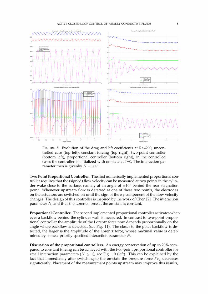
FIGURE 5. Evolution of the drag and lift coefficients at Re=200, uncon-trolled case (top left), constant forcing (top right), two-point controller(bottom left), proportional controller (bottom right), in the controlledcases the controller is initialized with on-state at T=0. The interaction pa-rameter then is givenby N = 0.43.
Two Point Proportional Controller. The first numerically implemented proportional con-troller requires that the (signed) flow velocity can be measured at two points in the cylin-der wake close to the surface, namely at an angle of ±10 behind the rear stagnationpoint. Whenever upstream flow is detected at one of these two points, the electrodeson the actuators are switched on until the sign of the x1-component of the flow velocitychanges. The design of this controller is inspired by the work of Chen [2]. The interactionparameter N , and thus the Lorentz force at the on-state is constant.
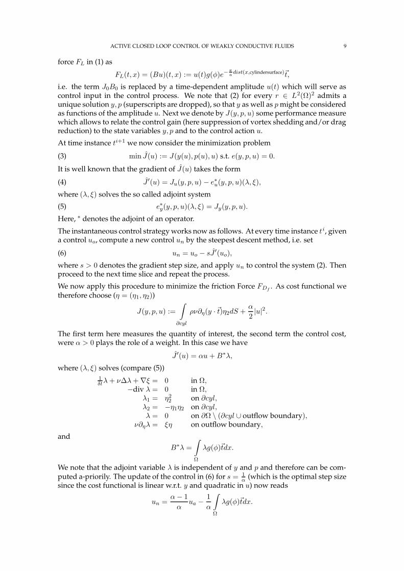
Proportional Controller. The second implemented proportional controller activates when-ever a backflow behind the cylinder wall is measured. In contrast to two-point propor-tional controller the amplitude of the Lorentz force now depends proportionally on theangle where backflow is detected, (see Fig. 11). The closer to the poles backflow is de-tected, the larger is the amplitude of the Lorentz force, whose maximal value is deter-mined by some a-priorily specified interaction parameter N .
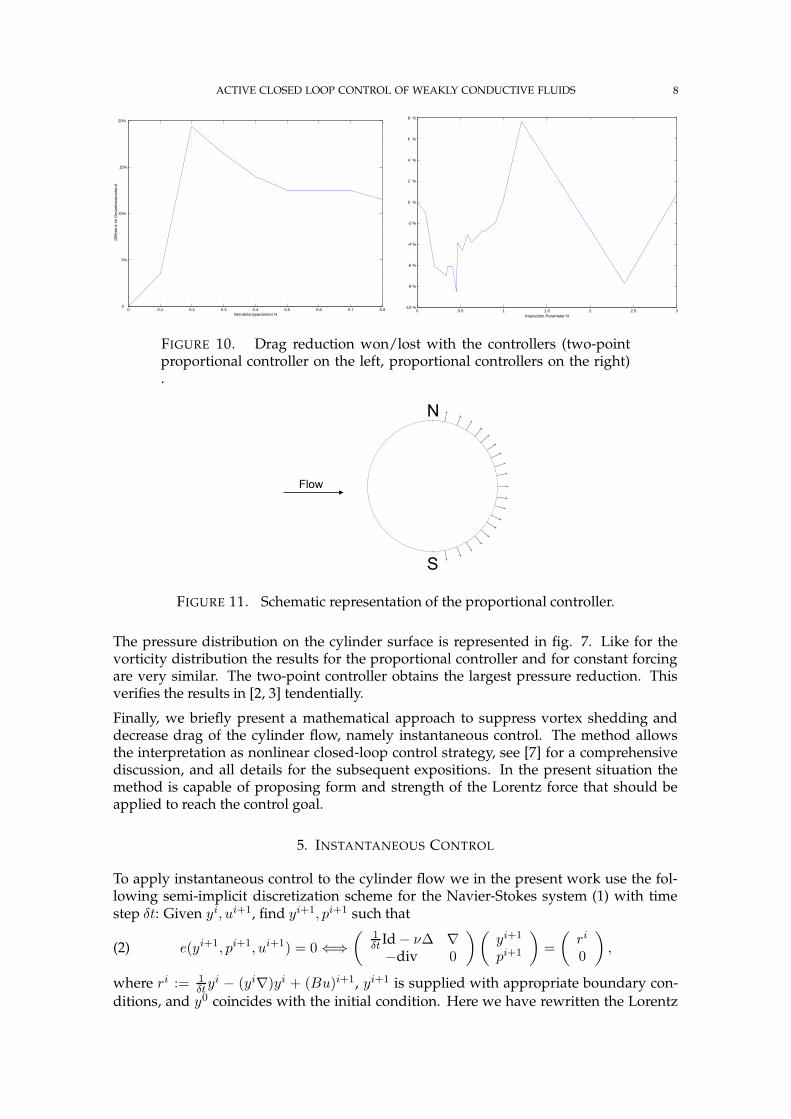
Discussion of the proportional controllers. An energy conservation of up to 20% com-pared to constant forcing can be achieved with the two-point proportional controller forsmall interaction parameters (N ≤ 1), see Fig. 10 (left). This can be explained by thefact that immediately after switching to the on-state the pressure force FDp decreasessignificantly. Placement of the measurement points upstream may improve this results,
ACTIVE CLOSED LOOP CONTROL OF WEAKLY CONDUCTIVE FLUIDS 6
0 0.2 0.4 0.6 0.8 1 1.2 2 3 4 5 6−4
−3.5
−3
−2.5
−2
−1.5
−1
−0.5
0
0.5
1
1.5
N
Cd
Comparison with Grundmann & Posdziech´s results
Pressure
Friction
EM−Thrust
Total
FIGURE 6. Dependency of the drag coefficients on the interaction param-eter at Re=200, Comparison with Grundmann/Posdziechs’ results.
0 pi/2 pi-5
-4
-3
-2
-1
0
1
2
Pressure distribution, Re=200, Block Profile
Constant Forcing, N=0.45No Forcing2 Point Controller N=0.43Proportional Controller N=0.4
FIGURE 7. Pressure distribution on the cylinder surface from the front tothe rear stagnation point: uncontrolled case, constant forcing, two pointproportional controller, and proportional controller, N =0.43 in all con-trolled examples.
as separation is detected earlier. In the thrust region (N > 1.3, not represented) thetwo-point proportional controller supplies no more energy conservation. For small in-teraction parameters (N ≤ 1) the proportional controller is not capable of reducing the
ACTIVE CLOSED LOOP CONTROL OF WEAKLY CONDUCTIVE FLUIDS 7
0 pi/2 pi
0
100
200
300
400
500
600
700
800
900
1000
Vorticitydistribution, Re=200, Block Profile
Constant Forcing, N=0.45 constNo Forcing2 Point Controller N=0.43Proportional Controller N=0.4
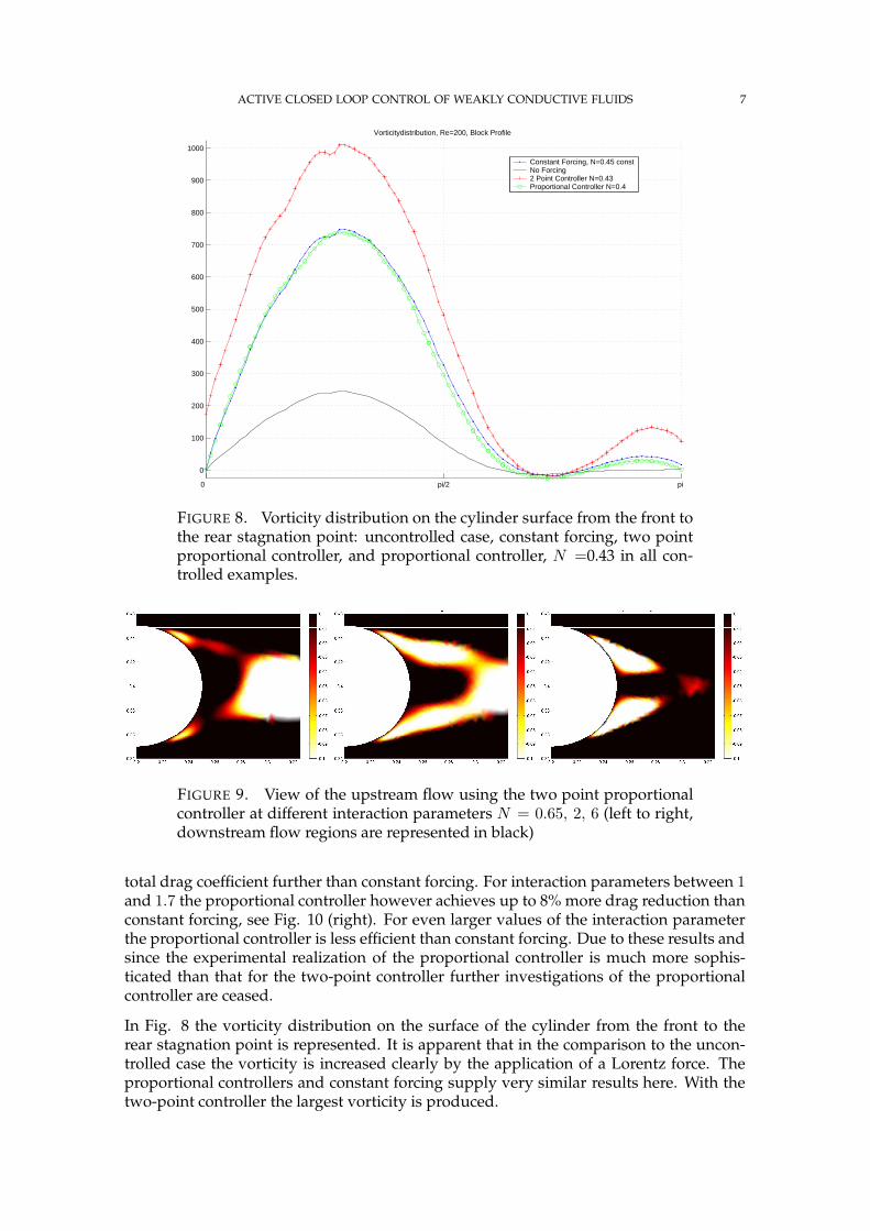
FIGURE 8. Vorticity distribution on the cylinder surface from the front tothe rear stagnation point: uncontrolled case, constant forcing, two pointproportional controller, and proportional controller, N =0.43 in all con-trolled examples.
FIGURE 9. View of the upstream flow using the two point proportionalcontroller at different interaction parameters N = 0.65, 2, 6 (left to right,downstream flow regions are represented in black)
total drag coefficient further than constant forcing. For interaction parameters between 1and 1.7 the proportional controller however achieves up to 8% more drag reduction thanconstant forcing, see Fig. 10 (right). For even larger values of the interaction parameterthe proportional controller is less efficient than constant forcing. Due to these results andsince the experimental realization of the proportional controller is much more sophis-ticated than that for the two-point controller further investigations of the proportionalcontroller are ceased.
In Fig. 8 the vorticity distribution on the surface of the cylinder from the front to therear stagnation point is represented. It is apparent that in the comparison to the uncon-trolled case the vorticity is increased clearly by the application of a Lorentz force. Theproportional controllers and constant forcing supply very similar results here. With thetwo-point controller the largest vorticity is produced.
ACTIVE CLOSED LOOP CONTROL OF WEAKLY CONDUCTIVE FLUIDS 8
0 0.1 0.2 0.3 0.4 0.5 0.6 0.7 0.80
5%
10%
15%
20%
Interaktionsparameter N
Diff
eren
z im
Ges
amtw
ider
stan
d
0 0.5 1 1.5 2 2.5 3-10 %
-8 %
-6 %
-4 %
-2 %
0 %
2 %
4 %
6 %
8 %
Interaction Parameter N
FIGURE 10. Drag reduction won/lost with the controllers (two-pointproportional controller on the left, proportional controllers on the right).
FIGURE 11. Schematic representation of the proportional controller.
The pressure distribution on the cylinder surface is represented in fig. 7. Like for thevorticity distribution the results for the proportional controller and for constant forcingare very similar. The two-point controller obtains the largest pressure reduction. Thisverifies the results in [2, 3] tendentially.
Finally, we briefly present a mathematical approach to suppress vortex shedding anddecrease drag of the cylinder flow, namely instantaneous control. The method allowsthe interpretation as nonlinear closed-loop control strategy, see [7] for a comprehensivediscussion, and all details for the subsequent expositions. In the present situation themethod is capable of proposing form and strength of the Lorentz force that should beapplied to reach the control goal.
5. INSTANTANEOUS CONTROL
To apply instantaneous control to the cylinder flow we in the present work use the fol-lowing semi-implicit discretization scheme for the Navier-Stokes system (1) with timestep δt: Given yi, ui+1, find yi+1, pi+1 such that
(2) e(yi+1, pi+1, ui+1) = 0 ⇐⇒
(
1δt
Id − ν∆ ∇−div 0
)(
yi+1
pi+1
)
=
(
ri
0
)
,
where ri := 1δt
yi − (yi∇)yi + (Bu)i+1, yi+1 is supplied with appropriate boundary con-ditions, and y0 coincides with the initial condition. Here we have rewritten the Lorentz
ACTIVE CLOSED LOOP CONTROL OF WEAKLY CONDUCTIVE FLUIDS 9
force FL in (1) as
FL(t, x) = (Bu)(t, x) := u(t)g(φ)e−πa
dist(x,cylindersurface)~t,
i.e. the term J0B0 is replaced by a time-dependent amplitude u(t) which will serve ascontrol input in the control process. We note that (2) for every r ∈ L2(Ω)2 admits aunique solution y, p (superscripts are dropped), so that y as well as p might be consideredas functions of the amplitude u. Next we denote by J(y, p, u) some performance measurewhich allows to relate the control gain (here suppression of vortex shedding and/or dragreduction) to the state variables y, p and to the control action u.
At time instance ti+1 we now consider the minimization problem
(3) min J(u) := J(y(u), p(u), u) s.t. e(y, p, u) = 0.
It is well known that the gradient of J(u) takes the form
(4) J ′(u) = Ju(y, p, u) − e∗u(y, p, u)(λ, ξ),
where (λ, ξ) solves the so called adjoint system
(5) e∗y(y, p, u)(λ, ξ) = Jy(y, p, u).
Here, ∗ denotes the adjoint of an operator.
The instantaneous control strategy works now as follows. At every time instance ti, givena control uo, compute a new control un by the steepest descent method, i.e. set
(6) un = uo − sJ ′(uo),
where s > 0 denotes the gradient step size, and apply un to control the system (2). Thenproceed to the next time slice and repeat the process.
We now apply this procedure to minimize the friction Force FDf. As cost functional we
therefore choose (η = (η1, η2))
J(y, p, u) :=
∫
∂cyl
ρν∂η(y · ~t)η2dS +α
2|u|2.
The first term here measures the quantity of interest, the second term the control cost,were α > 0 plays the role of a weight. In this case we have
J ′(u) = αu + B∗λ,
where (λ, ξ) solves (compare (5))1δt
λ + ν∆λ + ∇ξ = 0 in Ω,
−div λ = 0 in Ω,
λ1 = η22 on ∂cyl,
λ2 = −η1η2 on ∂cyl,
λ = 0 on ∂Ω \ (∂cyl ∪ outflow boundary),ν∂ηλ = ξη on outflow boundary,
andB∗λ =
∫
Ω
λg(φ)~tdx.
We note that the adjoint variable λ is independent of y and p and therefore can be com-puted a-priorily. The update of the control in (6) for s = 1
α(which is the optimal step size
since the cost functional is linear w.r.t. y and quadratic in u) now reads
un =α − 1
αua −
1
α
∫
Ω
λg(φ)~tdx.
ACTIVE CLOSED LOOP CONTROL OF WEAKLY CONDUCTIVE FLUIDS 10
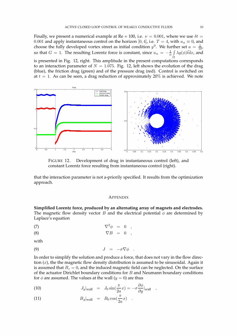
Finally, we present a numerical example at Re = 100, i.e. ν = 0.001, where we use δt =0.001 and apply instantaneous control on the horizon [0, 4], i.e. T = 4, with ua ≡ 0, andchoose the fully developed vortex street as initial condition y0. We further set a = 1
10 ,so that G = 1. The resulting Lorentz force is constant, since un = − 1
α
∫
Ω
λg(φ)~tdx, and
is presented in Fig. 12, right. This amplitude in the present computations correspondsto an interaction parameter of N = 1.075. Fig. 12, left shows the evolution of the drag(blue), the friction drag (green) and of the pressure drag (red). Control is switched onat t = 1. As can be seen, a drag reduction of approximately 20% is achieved. We note
0 0.5 1 1.5 2 2.5 3 3.5 40
0.5
1
1.5
time
Drag
total dragpressure dragfriction drag
0 0.05 0.1 0.15 0.2 0.25 0.3 0.35 0.4 0.45 0.50.2
0.4
0.6
FIGURE 12. Development of drag in instantaneous control (left), andconstant Lorentz force resulting from instantaneous control (right).
that the interaction parameter is not a-priorily specified. It results from the optimizationapproach.
APPENDIX
Simplified Lorentz force, produced by an alternating array of magnets and electrodes.The magnetic flow density vector B and the electrical potential φ are determined byLaplace’s equation
∇2φ = 0 ,(7)∇B = 0 ,(8)
with
J = −σ∇φ .(9)
In order to simplify the solution and produce a force, that does not vary in the flow direc-tion (x), the the magnetic flow density distribution is assumed to be sinusoidal. Again itis assumed that Bz = 0, and the induced magnetic field can be neglected. On the surfaceof the actuator Dirichlet boundary conditions for B and Neumann boundary conditionsfor φ are assumed. The values at the wall (y = 0) are thus
Jy|wall = J0 sin(π
2ax) = −σ
∂φ
∂y|wall ,(10)
By|wall = B0 cos(π
2ax) .(11)
ACTIVE CLOSED LOOP CONTROL OF WEAKLY CONDUCTIVE FLUIDS 11
The domain (7)-(9) is a channel with height of 2δ with insulating upper wall (i.e. By=2δ|wall =0, and Jy=2δ |wall = 0. The current density and flow density distributions are
Jx(x, y) = −J0
tanh(πaδ)
cos(π
2ax)[− tanh(
π
aδ) sinh(
π
2ay)] ,(12)
Jy(x, y) = −J0
tanh(πaδ)
sin(π
2ax)[− tanh(
π
aδ) cosh(
π
2ay)] ,(13)
Bx(x, y) = −B0 sin(π
2ax)[sinh(
π
2ay) −
cosh( π2a
y)
tanh( π2a
δ)] ,(14)
By(x, y) = −B0 cos(π
2ax)[cosh(
π
2ay) −
sinh( π2a
y)
tanh( π2a
δ)] .(15)
By taking the cross product of the current density and the magnetic flow density theresulting strength acts in x direction only, is thus a function of the wall-normal distancey only
(16) fz = J0B0[sinh(π
2ay) −
cosh( π2a
y)
tanh( π2a
δ)] × [cosh(
π
2ay) −
sinh( π2a
y)
tanh( π2a
δ)] .
For δa→ ∞
(17) fi = δi3J0B0 exp(−π
ay) .
REFERENCES
[1] K. Afanasiev: Stabilitätsanalyse, niedrigdimensionale Modellierung und optimale Kontrolle derKreiszylinderumströmung, Dissertation, TU Dresden 2001
[2] Z. Chen: Electro-Magnetic Control of Cylinder Wake, Dissertation,New Jersey Institute of Technology, May2001
[3] Z. Chen, N. Aubry: Communications in Nonlinear Science and Numerical Simulation, 2003[4] T. Berger, J. Kim, C. Lee, J. Lim: Turbulent boundary layer control utilizing the Lorentz force, Physics of
Fluids, Vol 12 #3, March 2000, pp. 631-649[5] M. Gad-el-Hak: Modern Developments in Flow Control. In: Appl. Mech. Rev. 49 (1996), pp365-379[6] R.D. Henderson: Details of the drag curve near the onset of vortex shedding, Aeronautics and Applied Math-
ematics, California Institute of Technology, pp. 2102-2104, 1995[7] M. Hinze: Optimal and instantaneous control of the instationary Navier-Stokes equations, Habilitation thesis
(2000), Fachbereich Mathematik, Technische Universität Berlin.[8] M.D. Gunzburger, Perspectives of flow control and Optimization, Siam, 2003[9] P. Poncet: Phys. Fluids 14, 2021-2023, 2002
[10] P. Poncet, P. Koumoutsakos: Proceedings of The Fourteenth International OFFSHORE AND POLARENGINEERING CONFERENCE, 2004
[11] O. Posdziech, R. Grundmann: Electromagnetic control of seawater flow around circular cylinders, Eur. J.Mech. B - Fluids 20, 2001, pp. 255-274
[12] T. Weier, Fey, G. Gerbeth, G. Mutschke, G. Avilov: Boundary layer control by means of electromagnetic forces.ERCOFTAC Bulletin 44 2000, pp.36-40
[13] T. Weier, G. Gerbeth, G. Mutschke, O. Lielausis, G. Lammers: Control of Flow Separation Using Electro-magnetic Forces, SFB 609 Preprint 2004-03
[14] T. Weier, J. Fey, G. Gerbeth, G. Mutschke, O. Lielausis, G. Platacis: Boundary layer control by means of wallparallel Lorentz forces. Magnetohydrodynamics . 2001. Vol. 37, No. 1/2, pp. 177-186
[15] T. Weier, G. Gerbeth, G. Mutschke, G. Platacis, O. Lielausis: Experiments on cylinder wake stabilizationin an electrolyte solution by means of electromagnetic forces localized on the cylinder surface. ExperimentalThermal and Fluid Science 16 (1998), pp.84-91
E-mail address: [email protected],[email protected]
URL: http://www.math.tu-dresden.de/~hinze