shadow prices - 國立臺灣大學
TRANSCRIPT

Author Name
Shadow Prices
Joseph Tao-yi Wang2019/9/11
(Lecture 2, Micro Theory I)
9/11/2019 Shadow PricesJoseph Tao-yi Wang

Author Name
A Peak-Load Pricing Problem
• Consider the problem faced by Chunghwa Telecom (CHT):
• By building base stations, CHT can provide cell phone service to a certain region– An establish network can provide service both in
the day and during the night
–Marginal cost is low (zero?!); setup cost is huge
• Marketing research reveal unbalanced demand– Day – peak; Night – off-peak (or vice versa?)
9/11/2019 Shadow PricesJoseph Tao-yi Wang

Author Name
A Peak-Load Pricing Problem
• If you are the CEO of CHT, how would you price usage of your service?
– Price day and night the same (or different)?
• Economic intuition should tell you to set off-peak prices lower than peak prices
– But how low?
• All new 4G services (LTE) are facing a similar problem now...
9/11/2019 Shadow PricesJoseph Tao-yi Wang

Author Name
More on Peak-Load Pricing
• Other similar problems include:
– How should Taipower price electricity in the summer and winter?
– How should a theme park set its ticket prices for weekday and weekends?
• Even if demand estimations are available, you will still need to do some math to find optimal prices...
– Either to maximize profit or social welfare
9/11/2019 Shadow PricesJoseph Tao-yi Wang

Author Name
A Peak-Load Pricing Problem
• Back to CHT:
• Capacity constraints:
• CHT's Cost function:
• Demand for cell phone service:
• Total Revenue:
9/11/2019 Shadow PricesJoseph Tao-yi Wang

Author Name
A Peak-Load Pricing Problem
• The monopolist profit maximization problem:
• How do you solve this problem?
• When does FOC guarantee a solution?
• What does the Lagrange multiplier mean?
• What should you do when FOC "fails"?
9/11/2019 Shadow PricesJoseph Tao-yi Wang

Author Name
Need: Lagrange Multiplier Method
1. Write Constraints as
2. Shadow prices
• Lagrangian
• FOC:
9/11/2019 Shadow PricesJoseph Tao-yi Wang

Author Name
Solving Peak-Load Pricing
• The monopolist profit maximization problem:
• The Lagrangian is
9/11/2019 Shadow PricesJoseph Tao-yi Wang

Author Name
Solving Peak-Load Pricing
• FOC:
9/11/2019 Shadow PricesJoseph Tao-yi Wang

Author Name
Solving Peak-Load Pricing
• For positive production, FOC becomes:
9/11/2019 Shadow PricesJoseph Tao-yi Wang
Author Name
Solving Peak-Load Pricing
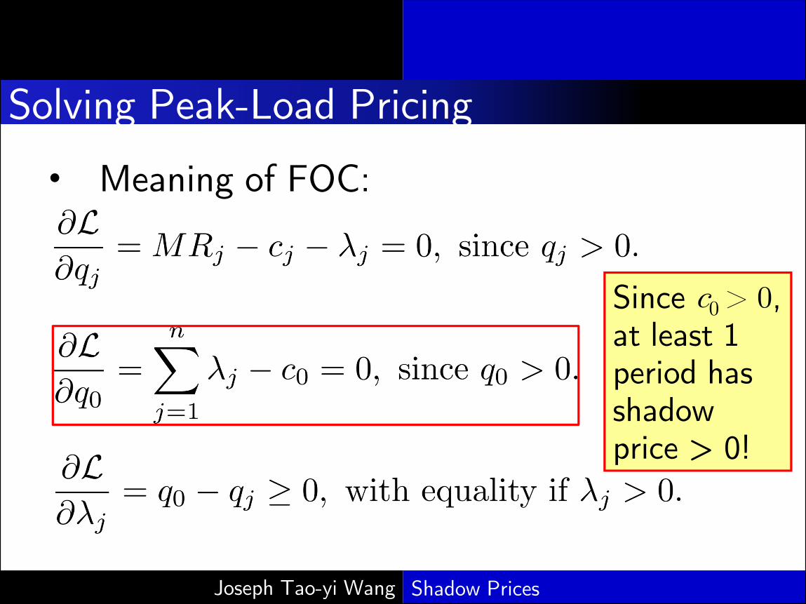
• Meaning of FOC:
9/11/2019 Shadow PricesJoseph Tao-yi Wang
Since c0 > 0, at least 1 period has shadow price > 0!

Author Name
Solving Peak-Load Pricing
• Meaning of FOC:
9/11/2019 Shadow PricesJoseph Tao-yi Wang
Hit capacity at positive
shadow price!
Off-peak shadow price = 0

Author Name
Solving Peak-Load Pricing
• Meaning of FOC:
9/11/2019 Shadow PricesJoseph Tao-yi Wang
Peak periods share capacity cost via shadow price
Peak MR = MC + capacity cost
Off-peak: MR=MC!

Author Name
Solving Peak-Load Pricing
• Economic Insight of FOC:
• Marginal decision of the manager: MR = MC
• Off-peak: MR = operating MC
– Since didn't hit capacity
• Peak: Need to increase capacity
– MR of all peak periods =
cost of additional capacity
+ operating MC of all peak periods
• What's the theory behind this?
9/11/2019 Shadow PricesJoseph Tao-yi Wang

Author Name
• Single Constraint Problem:
• Interpretation: a profit maximizing firm
– Produce non-negative output
– Subject to resource constraint
• Example: linear constraint
• Each unit of requires units of resource .
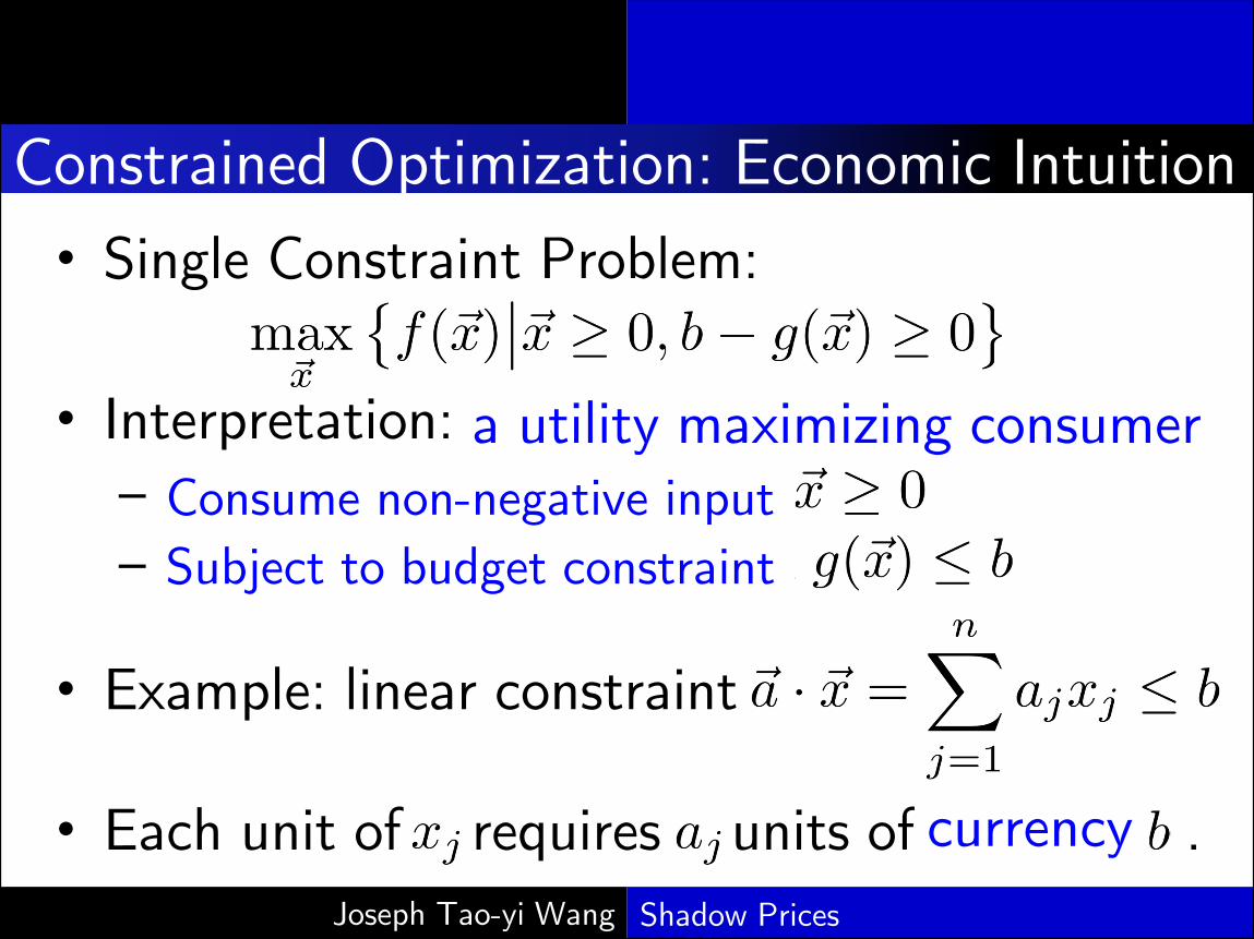
Constrained Optimization: Economic Intuition
9/11/2019 Shadow PricesJoseph Tao-yi Wang
Author Name
• Single Constraint Problem:
• Interpretation: a profit maximizing firm
– Produce non-negative output
– Subject to resource constraint
• Example: linear constraint
• Each unit of requires units of resource .
Constrained Optimization: Economic Intuition
9/11/2019 Shadow PricesJoseph Tao-yi Wang
a utility maximizing consumer
Consume non-negative input
Subject to budget constraint
currency

Author Name
Constrained Optimization: Economic Intuition
• Suppose solves the problem
• If one increases , profit changes by
• Additional resources needed:
• Cost of additional resources:
– (Market/shadow price is )
• Net gain of increasing is
9/11/2019 Shadow PricesJoseph Tao-yi Wang

Author Name
Necessary Conditions for
• Firm will increase if marginal net gain
– i.e. If is optimal
• Firm will decrease if marginal net gain (unless is already zero)
– i.e.
9/11/2019 Shadow PricesJoseph Tao-yi Wang
Author Name
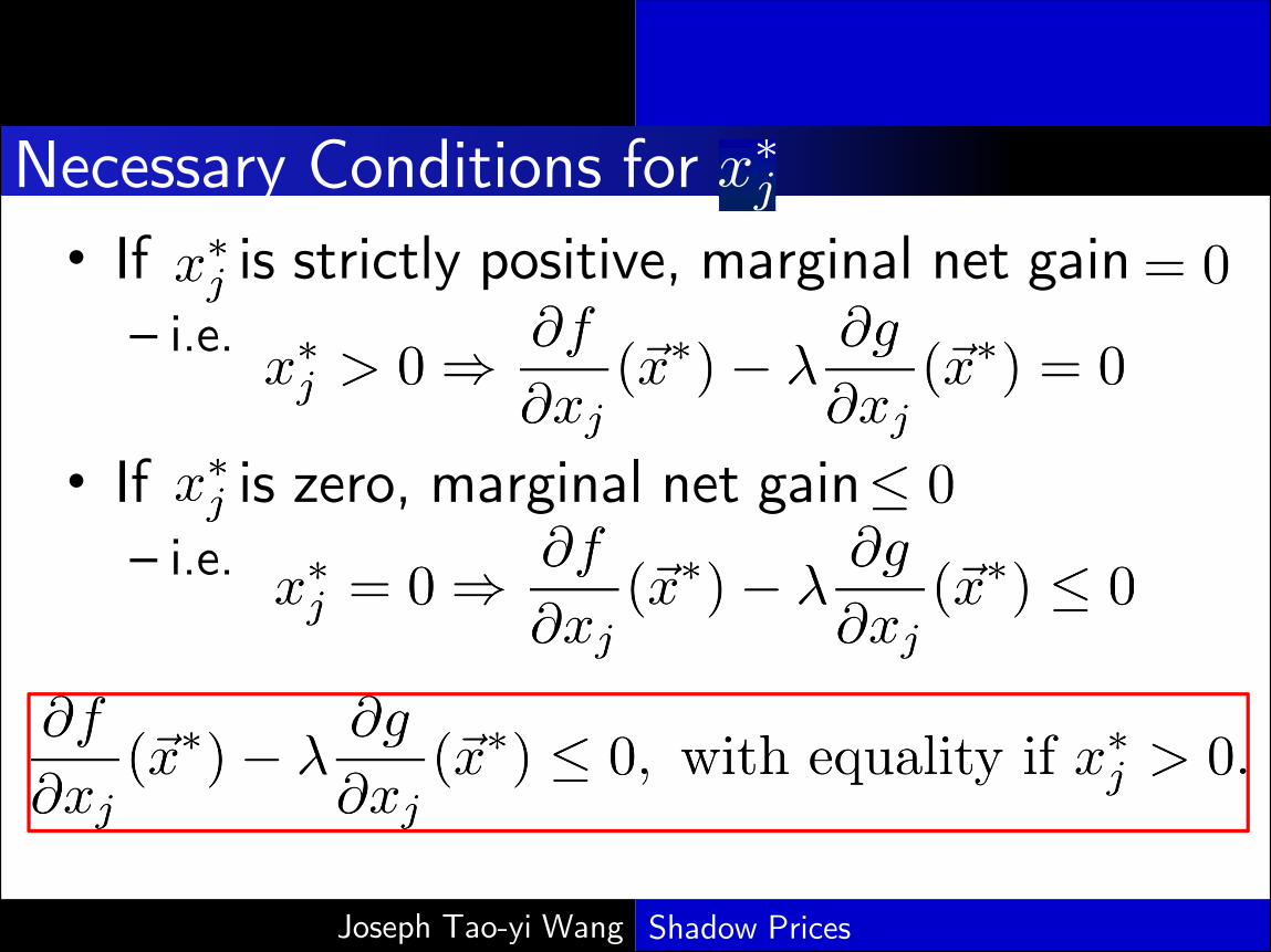
Necessary Conditions for
• If is strictly positive, marginal net gain
– i.e.
• If is zero, marginal net gain
– i.e.
9/11/2019 Shadow PricesJoseph Tao-yi Wang

Author Name
Necessary Conditions for
• If resource doesn't bind, opportunity cost
– i.e.
• Or, in other words,
– This is logically equivalent to the first statement.
9/11/2019 Shadow PricesJoseph Tao-yi Wang

Author Name
Lagrange Multiplier Method
1. Write constraint as
2. Lagrange multiplier = shadow price
• Lagrangian
• FOC:
9/11/2019 Shadow PricesJoseph Tao-yi Wang
Author Name
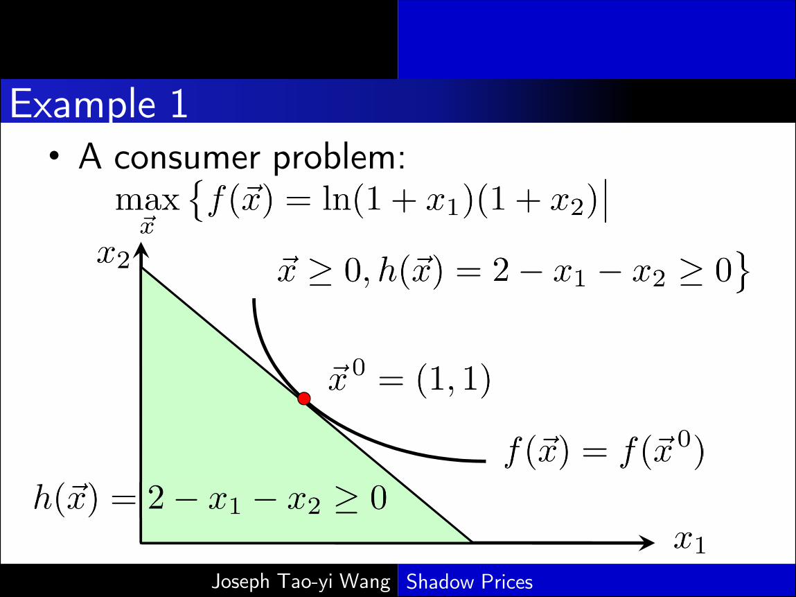
Example 1
• A consumer problem:
9/11/2019 Shadow PricesJoseph Tao-yi Wang

Author Name
Example 1
• Maximum at
• Lagrangian:
• FOC:
9/11/2019 Shadow PricesJoseph Tao-yi Wang

Author Name
Lagrange Multiplier w/ Multiple Constraints
1. Write Constraints as
2. Shadow prices
• Lagrangian
• FOC:
9/11/2019 Shadow PricesJoseph Tao-yi Wang

Author Name
When Intuition Breaks Down? Example 2
• A "new" problem:
9/11/2019 Shadow PricesJoseph Tao-yi Wang
Author Name
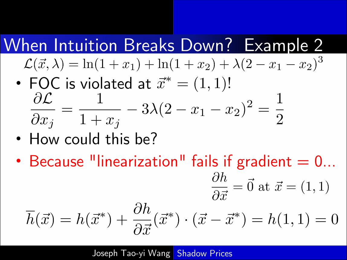
When Intuition Breaks Down? Example 2
• FOC is violated at
• How could this be?
• Because "linearization" fails if gradient = 0...
9/11/2019 Shadow PricesJoseph Tao-yi Wang

Author Name
Other Break Downs? See Example 3
9/11/2019 Shadow PricesJoseph Tao-yi Wang
Author Name
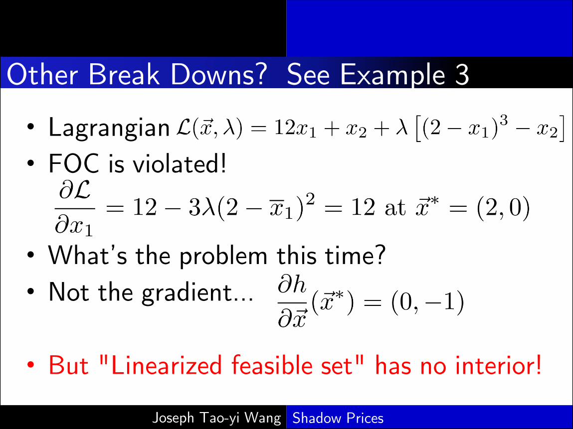
Other Break Downs? See Example 3
• Lagrangian
• FOC is violated!
• What's the problem this time?
• Not the gradient...
• But "Linearized feasible set" has no interior!
9/11/2019 Shadow PricesJoseph Tao-yi Wang
Author Name
Other Break Downs? See Example 3
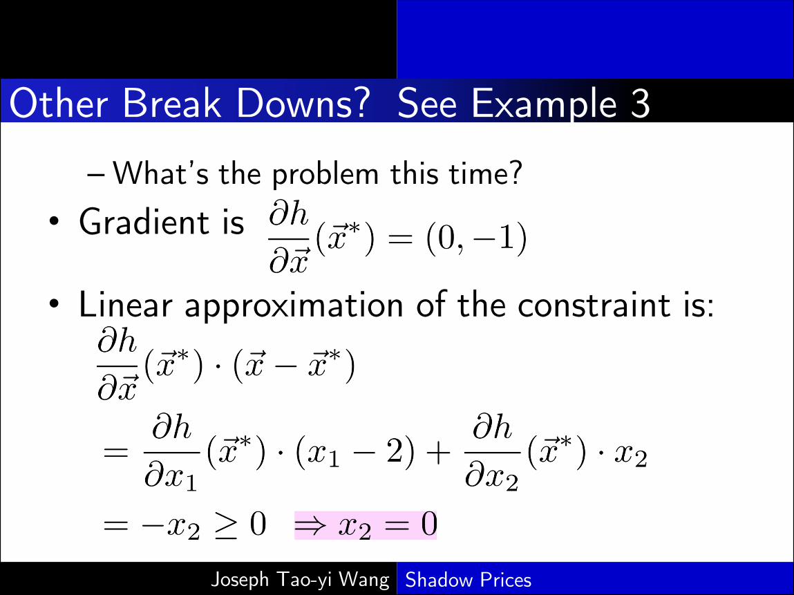
–What's the problem this time?
• Gradient is
• Linear approximation of the constraint is:
9/11/2019 Shadow PricesJoseph Tao-yi Wang

Author Name
Other Break Downs? See Example 3
Joseph Tao-yi Wang Shadow Prices
Linearized Feasible Set

Author Name
Linearized Feasible Set
• Set of constraints binding at :
– For
• Replace binding constraints by linear approx.
• These constraints also bind, and
– since
9/11/2019 Shadow PricesJoseph Tao-yi Wang

Author Name
Linearized Feasible Set
• Note: These are "true" constraints if gradient
• = Linearized Feasible Set
= Set of non-negative vectors satisfying
9/11/2019 Shadow PricesJoseph Tao-yi Wang

Author Name
Constraint Qualifications
• Set of feasible vectors:
• Constraint Qualifications hold at if
(i) Binding constraints have non-zero gradients
(ii) The linearized feasible set at has a non-empty interior.
– CQ guarantees FOC to be necessary conditions
9/11/2019 Shadow PricesJoseph Tao-yi Wang
Author Name
Proposition 1.2-1 Kuhn-Tucker Conditions
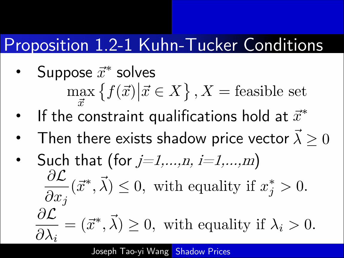
• Suppose solves
• If the constraint qualifications hold at
• Then there exists shadow price vector
• Such that (for j=1,...,n, i=1,...,m)
9/11/2019 Shadow PricesJoseph Tao-yi Wang

Author Name
Lemma 1.2-2 [Special Case] Quasi-Concave
• If for each binding constraint at , is quasi-concave and
• Then,
– Tangent Hyperplanes
– = Supporting Hyperplanes!
• Hence, if has a non-empty interior, then so does the linearized set
– Thus we have...
9/11/2019 Shadow PricesJoseph Tao-yi Wang

Author Name
Prop 1.2-3 [Quasi-Concave] Constraint Qualif.
• Suppose feasible set has non-empty interior
• Constraint Qualifications hold at if
• Binding constraints are quasi-concave,
• And the gradient
9/11/2019 Shadow PricesJoseph Tao-yi Wang
Author Name
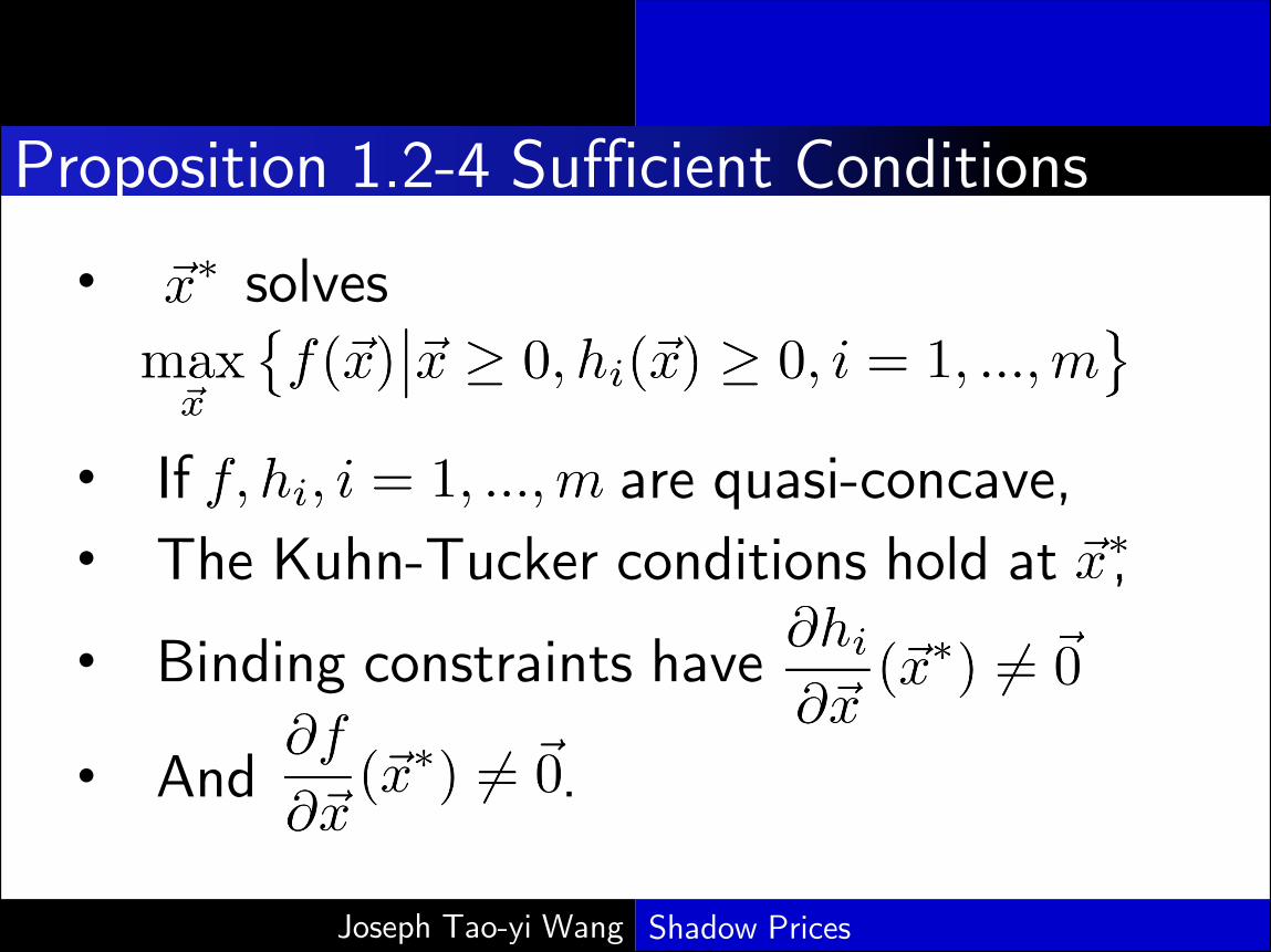
Proposition 1.2-4 Sufficient Conditions
• solves
• If are quasi-concave,
• The Kuhn-Tucker conditions hold at ,
• Binding constraints have
• And .
9/11/2019 Shadow PricesJoseph Tao-yi Wang

Author Name
Summary of 1.2
• Consumer = Producer
• Lagrange multiplier = Shadow prices
• FOC = "MR – MC = 0": Kuhn-Tucker
• When does this intuition fail?– Gradient = 0
– Linearized feasible set has no interior
Constraint Qualification: when it flies…– CQ for quasi-concave constraints
• Sufficient Conditions (Proof in Section 1.4)
9/11/2019 Shadow PricesJoseph Tao-yi Wang

Author Name
Summary of 1.2
• Peak-Load Pricing requires Kuhn-Tucker
• MR= "effective" MC
• Off-peak shadow price (for capacity) = 0
• Peak periods share additional capacity cost
• Can you think of real world situations that requires something like peak-load pricing?– After you start your new job making $$$$...
• Homework: Exercise 1.2-2 (Optional 1.2-3)
9/11/2019 Shadow PricesJoseph Tao-yi Wang