shapes of polyhedra and triangulations of the sphere · pdf fileshapes of polyhedra and...
TRANSCRIPT
ISSN 1464-8997 (on line) 1464-8989 (printed) 511
Geometry & Topology Monographs
Volume 1: The Epstein birthday schrift
Pages 511–549
Shapes of polyhedra and triangulations of the sphere
William P Thurston
Abstract The space of shapes of a polyhedron with given total angles lessthan 2π at each of its n vertices has a Kahler metric, locally isometric tocomplex hyperbolic space CHn−3 . The metric is not complete: collisionsbetween vertices take place a finite distance from a nonsingular point. Themetric completion is a complex hyperbolic cone-manifold. In some inter-esting special cases, the metric completion is an orbifold. The concretedescription of these spaces of shapes gives information about the combi-natorial classification of triangulations of the sphere with no more than 6triangles at a vertex.
AMS Classification 51M20; 51F15, 20H15, 57M50
Keywords Polyhedra, triangulations, configuration spaces, braid groups,complex hyperbolic orbifolds
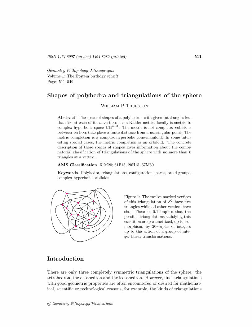
Figure 1: The twelve marked verticesof this triangulation of S2 have fivetriangles while all other vertices havesix. Theorem 0.1 implies that thepossible triangulations satisfying thiscondition are parametrized, up to iso-morphism, by 20–tuples of integersup to the action of a group of inte-ger linear transformations.
Introduction
There are only three completely symmetric triangulations of the sphere: thetetrahedron, the octahedron and the icosahedron. However, finer triangulationswith good geometric properties are often encountered or desired for mathemat-ical, scientific or technological reasons, for example, the kinds of triangulations
c© Geometry & Topology Publications
512 William P Thurston
popularized in modern times by Buckminster Fuller and used for geodesic domesand chemical ‘Buckyballs’.
There are procedures to refine and modify any triangulation of a surface untilevery vertex has either 5, 6 or 7 triangles around it, or with more effort, so thatthere are only 5 or 6 triangles if the surface has positive Euler characteristic, only6 triangles if the surface has zero Euler characteristic, or only 6 or 7 triangles ifthe surface has negative Euler characteristic. These conditions on triangulationsare combinatorial analogues of metrics of positive, zero or negative curvature.How systematically can they be understood?
In this paper, we will develop a global theory to describe all triangulations ofthe S2 such that each vertex has 6 or fewer triangles at any vertex. Here isone description:
Theorem 0.1 (Polyhedra are lattice points) There is a lattice L in complexLorentz space C(1,9) and a group Γ of automorphisms, such that triangulationsof non-negative combinatorial curvature are elements of L+/Γ, where L+ isthe set of lattice points of positive square-norm. The projective action of Γon complex hyperbolic space CH9 (the unit ball in C9 ⊂ CP9 ) has quotientof finite volume. The square of the norm of a lattice point is the number oftriangles in the triangulation.
A triangulation is non-negatively curved if there are never more than six trian-gles at a vertex. The theorem can be interpreted as describing certain concretecut-and-glue constructions for creating triangulations of non-negative curva-ture, starting from simple and easily-classified examples. The constructions areparametrized by choices of integers, subject to certain geometric constraints.The fact that Γ is a discrete group means that it is possible to dispensewith most of the constraints, except for an algebraic condition that a certainquadratic form is positive: any choice of integer parameters can be transformedby Γ to satisfy the geometric conditions, and the resulting triangulation isunique. Thus, the collection of all triangulations can be described either as aquotient space, in which identifications of the parameters are made algebraically,or as a fundamental domain (see section 7).
We will study combinatorial types of triangulations by using a metric whereeach triangle is a Euclidean equilateral triangle with sides of unit length. Thismetric is locally Euclidean everywhere except near vertices that have fewer than6 triangles.
It is helpful to consider these metrics as a special case of metrics on the spherewhich are locally Euclidean except at a finite number of points, which have
Geometry & Topology Monographs, Volume 1 (1998)
Shapes of polyhedra and triangulations of the sphere 513
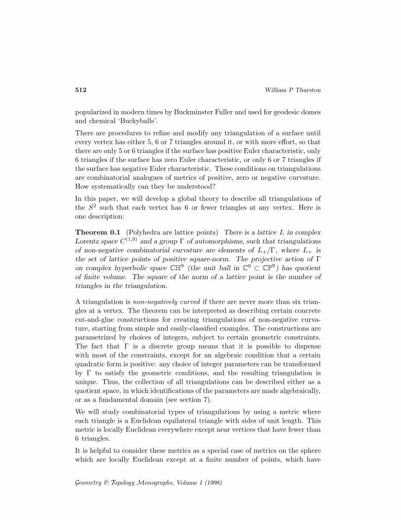
neighborhoods locally modelled on cones. A cone of cone-angle θ is a metricspace that can be formed, if θ ≤ 2π , from a sector of the Euclidean planebetween two rays that make an angle θ , by gluing the two rays together. Moregenerally, a cone of angle θ can be formed by taking the universal cover of theplane minus 0, reinserting 0, and then identifying modulo a transformationthat “rotates” by angle θ . The apex curvature of a cone of cone-angle θ is2π − θ .
A Euclidean cone metric on a surface satisfies the Gauss–
θ
Cone angle θ
Bonnet theorem, that is, the sum of the apex curvatures is2π times the Euler characteristic. This fact can be derivedfrom basic Euclidean geometry by subdividing the surface intotriangles and looking at the sum of angles of all trianglesgrouped in two different ways, by triangle or by vertex. It canalso be derived from the usual smooth Gauss–Bonnet formula
by rounding off the points, replacing a tiny neighborhood of each cone point bya smooth surface (for example part of a small sphere).
Theorem 0.2 (Cone metrics form cone manifold) Let k1, k2, . . . , kn [n > 3]be a collection of real numbers in the interval (0, 2π) whose sum is 4π . Thenthe set of Euclidean cone metrics on the sphere with cone points of curvature ki
and of total area 1 forms a complex hyperbolic manifold, whose metric comple-tion is a complex hyperbolic cone manifold of finite volume. This cone manifoldis an orbifold (that is, the quotient space of a discrete group) if and only if forany pair ki, kj whose sum s = ki + kj that is less than 2π , either
(i) (2π − s) divides 2π , or
(ii) ki = kj , and (2π − s)/2 = (π − ki) divides 2π .
The definition of “cone-manifold” in dimensions bigger than 2 will be givenlater.
This turns out to be closely related to work of Picard ([6], [7]) and Mostowand Deligne ([2], [3], [5]). Picard discovered many of the orbifolds; his studentLeVavasseur enumerated the class of groups Picard discovered, and they werefurther analyzed by Deligne and Mostow. Mostow discovered that condition(i) is not always required to obtain an orbifold and that (ii) is sufficient whenki = kj . However, the geometric interpretations were not apparent in thesepapers. It is possible to understand the quotient cone-manifolds quite concretelyin terms of shapes of polyhedra.
A version of this paper has circulated for a number of years as a preprint, whichfor a time was circulated as a Geometry Center preprint, and later revised as
Geometry & Topology Monographs, Volume 1 (1998)

514 William P Thurston
part of the xxx mathematics archive. In view of this history, some time warpis inevitable: for some parts of this paper, others may have have done furtherwork that is not here taken into account. I would like to thank Derek Holt,Igor Rivin, Chih-Han Sah and Rich Schwarz for mathematical comments andcorrections that I hope I have taken into account.
1 Triangulations of a hexagon
Let E be the standard equilateral triangulation of C by triangles of unit sidelength, where 0 and 1 are both vertices. The set Eis of vertices of E arecomplex numbers of the form m + pω , where ω = 1/2 +
√−3/2 is a primitive
6th root of unity. These lattice points form a subring of C, called the Eisensteinintegers, the ring of algebraic integers in the quadratic imaginary field Q(
√−3).
Figure 2: An Eisenstein lattice hexagon has the formof a large equilateral triangle of sidelength n , minusthree equilateral triangles that fit inside it of side-lengths p1 , p2 and p3 . An equilateral triangle of side-length n contains n2 unit equilateral triangles, so thehexagon has n2 − p2
1 − p22 − p2
3 triangles.
To warm up, we’ll analyze all possible shapes of Eisenstein lattice hexagons,with vertices in Eis and sides parallel (in order) with the sides of a standardhexagon. Note that any such hexagon with m triangles determines a non-negatively curved triangulation of the sphere with 2m triangles, formed bymaking a hexagonal envelope from two copies of the hexagon glued along theboundary.
If we circumscribe a lattice triangle T about our lattice hexagon H , this givesa description
H = T \ (S1 ∪ S2 ∪ S3) ,
where the Si are smaller equilateral triangles. If T has sidelength n and Si
has sidelength pi , then H contains
m = n2 − p21 − p2
2 − p23 (1)
triangles.
Geometry & Topology Monographs, Volume 1 (1998)

Shapes of polyhedra and triangulations of the sphere 515
All such hexagons are described by four integer parameters, subject to the 6inequalities
p1 ≥ 0 p2 ≥ 0 p3 ≥ 0
p1 + p2 ≤ n p2 + p3 ≤ n p3 + p1 ≤ n,
where strict inequalities give non-degenerate hexagons; if one or more inequalitybecomes an equality then one or more sides of the hexagon shrinks to length 0and the ‘hexagon’ becomes a pentagon, quadrilateral or triangle.
Figure 3: The space of shapes of hexagons is de-scribed by this polyhedron in hyperbolic 3–space;the faces represent hexagons degenerated to pen-tagons, and the edges represent degeneration toquadrilaterals. All dihedral angles are π/2. Thethree mid-level vertices are ideal vertices at infin-ity, and represent the three ways that hexagons canbecome arbitrarily long and skinny, while the topand bottom are finite vertices, representing the twoways that hexagons can degenerate to equilateraltriangles. The polyhedron has hyperbolic volume.91596559417 . . . .
The solutions are elements of the integer lattice inside a convex cone C ⊂R4 . This description can be extended to non-integer parameters, which thendetermine a size and shape for the hexagon, but not a triangulation. Equation(1) expresses the area, measured in triangles, as a quadratic form of signature(1, 3). The isometry group of any such a form is C2 × Isom(H3) (where C2
denotes the cyclic group of order 2).
The possible shapes of lattice hexagons (where rescaling is allowed) are para-metrized by a convex polyhedron H ⊂ H3 which is the projective image of theconvex cone C ⊂ R(1,3) . This polyhedron has three ideal vertices at infinity,which represent the three directions in which shapes of hexagons can tend to-ward infinity, by becoming long and skinny along one of three axes. In addition,there are two finite vertices (top and bottom), representing the two ways thata hexagon can degenerate to an equilateral triangle. All dihedral angles of thishyperbolic polyhedron are π/2. Four edges meet at each ideal vertex, whilethree edges meet at the finite vertices. Triangulations with m triangles arerepresented by a discrete set Hm ⊂ H . Figure 4 plots the count of how manyof these lattice hexagons there are with each possible area up to 1, 000. Oneindication of the relevance of hyperbolic geometry is that the average number
Geometry & Topology Monographs, Volume 1 (1998)

516 William P Thurston
200 400 600 800 1000
100
200
300
400
Figure 4: Left the weighted count of Eisenstein lattice hexagons containing up to1000 triangles, using orbifold weights 1/2k where k is the number of sides of ahexagon of length 0. The parameter space of shapes (figure 3) has hyperbolic vol-ume .91596559417 . . . (1/4 that of the Whitehead Link complement), so the num-ber of hexagons containing m triangles should grow on the average as the volumeof the intersection of C/2 with the shell in E(1,3) between radius
√m and
√m + 1,
.45798279709 · · · ∗ m , as indicated. Right The same data averaged over windows ofsize 49.
of hexagons of a given area is well estimated by the hyperbolic volume of theparameter space.
Figure 5: A butterfly operation moves one edge of a hexagon (left) across a butterfly-shaped quadrilateral of 0 area, yielding a new hexagon (right) of the same area. Theset of butterfly moves generate a discrete group of isometries of H3 , generated byreflections in the faces of the polyhedron H .
It’s interesting to note that H is the fundamental polyhedron for a discretegroup of isometries of H3 , since all dihedral angles equal π/2. This group canbe interpreted in terms of not necessarily simple hexagons in the Eisensteinlattice whose sides are parallel, in order, to those of the standard hexagon.A non-simple lattice hexagon wraps with integer degree around each trianglein the plane; its total area, using these integer weights, is given by the same
Geometry & Topology Monographs, Volume 1 (1998)
Shapes of polyhedra and triangulations of the sphere 517
quadratic form n2 −∑
p2i .
Reflection in a face of the polyhedron corresponds to a ‘butterfly move’, whichis described numerically by reversing the sign of the length of one of the edgesof the hexagon, and adjusting the two neighboring lengths so that the resultis a closed curve. Geometrically, the hexagon moves across a quadrilateralreminiscent of a butterfly, resulting in a new hexagon that algebraically enclosesthe same area as the original. Note that this operation fixes any hexagon wherethe given side has degenerated to have length 0—this is one of the faces ofthe polyhedron H . The operations for two sides of the hexagon that do notmeet commute with each other, and fix any shapes of hexagons where boththese sides have length 0. These shapes describe an edge of H , and since thereflections in adjacent faces commute, the angle must be π/2. Two adjacentsides of the hexagon cannot both have 0 length at once, so the 9 non-adjacentpairs of sides of the hexagon correspond 1–1 to the 9 edges of H .
Any solution to the equation 0 < m = n2 − p21 − p2
2 − p23 determines a not
necessarily simple hexagon of area m, which projects to a point in H3 . Bya sequence of butterfly moves, this point can be transformed to be inside thefundamental domain H . The resulting point inside H is uniquely determinedby the initial solution and does not depend on what sequence of butterfly moveswere used to get it there, since H is the quotient space (quotient orbifold) forthe group action as well as being its fundamental domain.
2 Triangulations of the sphere
Let P (n; k1, k2, . . . , ks) denote the set of isomorphism classes of “triangulations”of the sphere having exactly 2n triangles, where for each i there is one vertexincident to 6−ki triangles, and all remaining vertices are incident to 6 triangles.This paper will be limited to the non-negatively curved cases that 0 < ki ≤ 5.For there to be any actual triangulations we must have
∑
i ki = 12. We willuse the term “triangulation” throughout to refer to a space obtained by gluingtogether triangles by a pairing of their edges; thus, in the case ki = 5, two edgesof a triangle are folded together to form a vertex incident to a single triangle.Every triangulation of the sphere has an even number of triangles.
If T ∈ P (n; k1, . . . , ks), then there is a developing map DT from the universalcover T of T minus its singular vertices into E . Choose any triangle of T , andmap it to the triangle ∆(0, 1, ω). The developing map DT is now determined bya form of analytic continuation, so that it is a local isometry, mapping trianglesto triangles.
Geometry & Topology Monographs, Volume 1 (1998)
518 William P Thurston
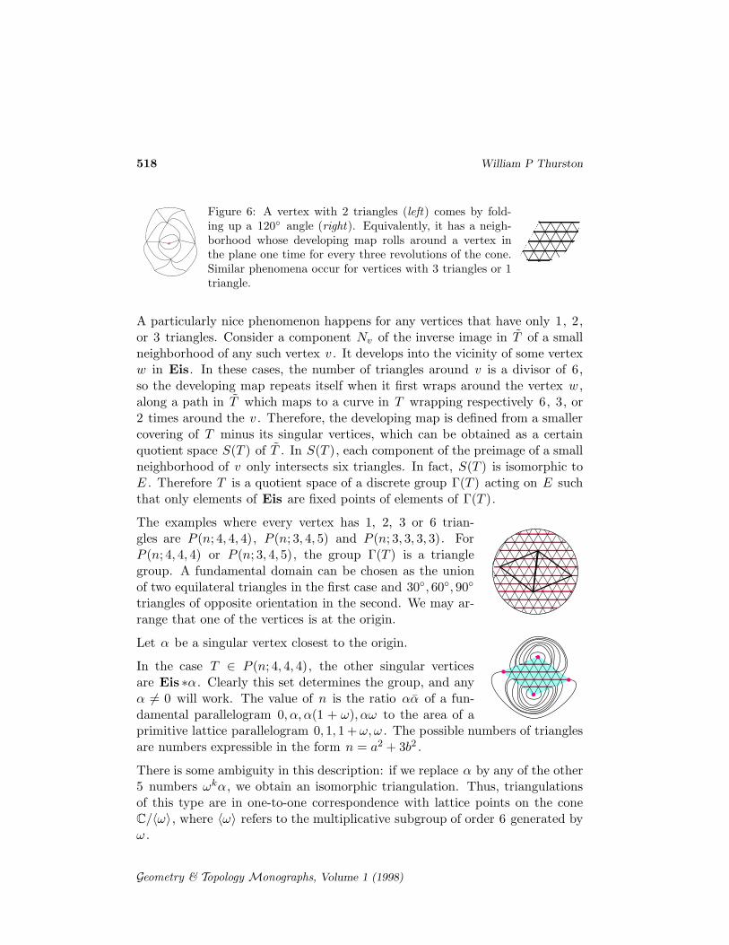
Figure 6: A vertex with 2 triangles (left) comes by fold-ing up a 120◦ angle (right). Equivalently, it has a neigh-borhood whose developing map rolls around a vertex inthe plane one time for every three revolutions of the cone.Similar phenomena occur for vertices with 3 triangles or 1triangle.
A particularly nice phenomenon happens for any vertices that have only 1, 2,or 3 triangles. Consider a component Nv of the inverse image in T of a smallneighborhood of any such vertex v . It develops into the vicinity of some vertexw in Eis. In these cases, the number of triangles around v is a divisor of 6,so the developing map repeats itself when it first wraps around the vertex w ,along a path in T which maps to a curve in T wrapping respectively 6, 3, or2 times around the v . Therefore, the developing map is defined from a smallercovering of T minus its singular vertices, which can be obtained as a certainquotient space S(T ) of T . In S(T ), each component of the preimage of a smallneighborhood of v only intersects six triangles. In fact, S(T ) is isomorphic toE . Therefore T is a quotient space of a discrete group Γ(T ) acting on E suchthat only elements of Eis are fixed points of elements of Γ(T ).
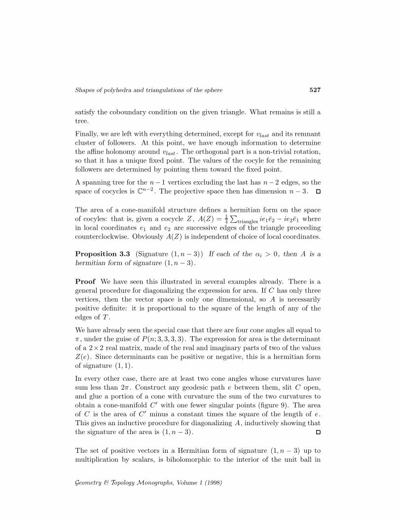
The examples where every vertex has 1, 2, 3 or 6 trian-gles are P (n; 4, 4, 4), P (n; 3, 4, 5) and P (n; 3, 3, 3, 3). ForP (n; 4, 4, 4) or P (n; 3, 4, 5), the group Γ(T ) is a trianglegroup. A fundamental domain can be chosen as the unionof two equilateral triangles in the first case and 30◦, 60◦, 90◦
triangles of opposite orientation in the second. We may ar-range that one of the vertices is at the origin.
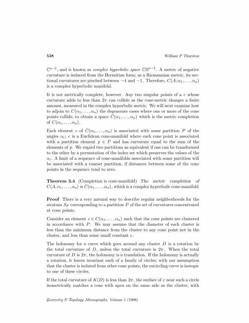
Let α be a singular vertex closest to the origin.
In the case T ∈ P (n; 4, 4, 4), the other singular verticesare Eis ∗α. Clearly this set determines the group, and anyα 6= 0 will work. The value of n is the ratio αα of a fun-damental parallelogram 0, α, α(1 + ω), αω to the area of aprimitive lattice parallelogram 0, 1, 1 + ω, ω . The possible numbers of trianglesare numbers expressible in the form n = a2 + 3b2 .
There is some ambiguity in this description: if we replace α by any of the other5 numbers ωkα, we obtain an isomorphic triangulation. Thus, triangulationsof this type are in one-to-one correspondence with lattice points on the coneC/〈ω〉, where 〈ω〉 refers to the multiplicative subgroup of order 6 generated byω .
Geometry & Topology Monographs, Volume 1 (1998)

Shapes of polyhedra and triangulations of the sphere 519
Figure 7: Developing a triangulation with 3 or 6 triangles at each vertex.
Similarly, in the case T ∈ P (n; 3, 4, 5), the vertices are of the form (m +p√−3)α, and n = 2αα . As before, α is well-defined only up to multiplica-
tion by powers of ω . In this case, if we replace α by ωkα, where k is odd, weget a different triangle group, but it has an isomorphic quotient space.
The case P (n; 3, 3, 3, 3) allows somewhat more variation. For a singular vertexx in Eis, let γx ∈ Γ(T ) be the rotation of order 2 about x. Then for any twoelements x and y , the product γxγ0γy is a 180◦ rotation about x+y . Therefore,the singular vertices form an additive subgroup of Eis. Any additive subgroupwill work. The subgroup is determined if we specify the sides α and β of afundamental parallelogram. If we express α and β as linear combinations ofthe generators 1 and ω for Eis, then the value of n is twice the determinantof the resulting two by two matrix. Every even number is achievable. Ofcourse, α and β are well-defined only up to change of basis for the latticeand up to multiplication by 6th roots of unity. Note that multiplication byω3 = −1 is also represented by a change of generators. A nice picture can beformed by considering the shape parameter z = β/α. The action of the groupSL(2, Z) on the set of shape parameters is the usual action by fractional lineartransformations on the upper half plane. Figure 8 illustrates the set of shapesobtainable for n = 246.
Let us now skip to a more complicated case, that of P (n; 2, 2, 2, 2, 2, 2), whichincludes the regular octahedron. We have already encountered a special case:the hexagonal envelopes of section 1 are examples of octahedra of this sort.
Just as a hexagon can be described by removing three small triangles from alarge triangle, there is a way to describe any element T ∈ P (n; 2, 2, 2, 2, 2, 2) bymodifying an element T ∈ P (m; 3, 3, 3), for some m.
Suppose T is any triangulation of the sphere with 6 vertices incident to fourtriangles, and the rest incident to 6.
Geometry & Topology Monographs, Volume 1 (1998)

520 William P Thurston
Figure 8: This is P (246; 3, 3, 3, 3), plotted in the Poincare disk model of H2 . Theelements of P (246; 3, 3, 3, 3) are small dots; the Voronoi diagram for these dots isshown, with one small dot inside each region. The position of the dot in H2 determinesthe shape of a tetrahedron triangulated by 246 equilateral triangles. Two dots whichdiffer by PSL(2, Z) represent the same shape. The shape does not always completelydetermine the triangulation—one also needs an angle for edges, that is, a lifting of thepoint to a certain line bundle over H2 .
Consider the associated cone metric C . We claim there is at least one wayto join the 6 cone points in pairs by three disjoint geodesic segments. Toconstruct such a pairing, first observe that any pair of cone points are joined byat least one geodesic: the shortest path between them is a geodesic. Note thatgeodesics can never pass through cone points with positive curvature, except attheir endpoints. We see that there is a collection of three not-necessarily disjointgeodesic segments joining the 6 points in pairs. Let {e, f, g} be such a collection
Geometry & Topology Monographs, Volume 1 (1998)

Shapes of polyhedra and triangulations of the sphere 521
Figure 9: Left If a Euclidean cone manifold is cut along a geodesic arc joining thetwo cone points of curvature α and β , the resulting figure is isometric to a region ina Euclidean cone manifold with a new cone point whose curvature is α + β (middle).This gives a recursive procedure to reduce the construction of compact Euclidean conemanifolds of non-positive curvature to ones having only three cone points. Right Anelement T ∈ P (n; 2, 2, 2, 2, 2, 2) can be reduced to T ′ ∈ P (n′; 3, 3, 3) by slitting 3 arcs,then extending.
of shortest possible length. In particular, e, f and g are shortest paths withtheir given endpoints. No pair of these edges can intersect: if they did, then bycutting and pasting, one would find that the four endpoints involved could bejoined in an alternate way by shorter paths.
Cut C along the three edges e, f and g , and consider the developing mapfor the resulting surface C ′ . At an endpoint of say e, the developing imagesubtends an angle of 120◦ ; a curve which wraps three times around e in a smallneighborhood develops to a curve wrapping once around the outside of a regularhexagon He in the plane. Let Ce be He modulo a rotation of order 3. If weglue Ce and the similarly constructed cones Cf and Cg to the cuts, we obtain anew cone-manifold C ′′ , with three cone points of order 3. The hexagon He hasits vertices on lattice points of Eis, so its center is also a lattice point of Eis.Therefore, C ′′ ∈ P (m; 4, 4, 4) for some m. Consequently, a general element ofP (n; 2, 2, 2, 2, 2, 2) is obtained by choosing some m bigger than n, choosing anelement of P (m; 4, 4, 4), and choosing three types of hexagons whose area intriangles adds to 6(m − n) such that when they are placed around the threeclasses of order 3 points in the plane, all their images are disjoint. Cut allthese hexagons out of the plane, divide by the (3, 3, 3) triangle group, and gluetogether the pair of edges coming from each hexagon. We can express this as achoice of four elements αi ∈ Eis, such that
α1α1 − α2α2 − α3α3 − α4α4 :
α1 is used to construct the original (3, 3, 3) triangle group, and the other αi ’sare vectors from the centers of the each of the hexagons to one of the vertices,
Geometry & Topology Monographs, Volume 1 (1998)

522 William P Thurston
Figure 10: This is an illustration of the construction of a generalized octahedron, thatis, an element of P (n; 2, 2, 2, 2, 2, 2). First, choose a 3, 3, 3 group acting in the planewith the fixed points of the elements of order 3 on lattice points of Eis. Then choosethree families of lattice hexagons invariant by the group, centered at the fixed points ofelements of order 3. Remove the hexagons, form the quotient by the group, and gluethe edges of the resulting slits together. Equivalently, you can glue the boundary of afundamental domain as illustrated.
yielding a triangulation
T (α1, α2, α3, α4) ∈ P (n; 2, 2, 2, 2, 2, 2).
The αi ’s are subject to an additional geometric condition, that the hexa-gons they define be embedded. The coordinates are only defined up to ageometrically-defined equivalence relation, having to do with the multiplicityof choices for e, f , and g . The easy observation is that when any of the αi aremultiplied by powers of ω , we obtain the same T . These coordinates make iteasy to automatically enumerate all examples, although it is somewhat harderto weed out repetitions. The geometric conditions can be nearly determinedfrom the norms: if |αi|+ |αj| < |α1|, for i 6= j ∈ {2, 3, 4}, then the hexagons aredisjoint; if this sum is greater than (2/
√3)|α1| = 1.1547 . . . |α1|, then two hexa-
gons intersect; otherwise, one needs to consider the picture. If |αi| < |α1|/3 fori > 1, then the three edges e, f and g are clearly the three shortest possibleedges; in general, the question is more complicated. The standard octahedron
Geometry & Topology Monographs, Volume 1 (1998)

Shapes of polyhedra and triangulations of the sphere 523
O ∈ P (4; 2, 2, 2, 2, 2, 2), for example, has an infinite number of descriptions, forexample O = T (2k + 1 + (−k + 2)ω, k + ω, k + ω, k + ω) for every k ≥ 0.
Another construction will be given in section 7 that can be used to search allpossibilities while weeding out repetition fairly efficiently.
3 Shapes of polyhedra
Any collection of n–dimensional Euclidean polyhedra whose (n−1)–dimensionalfaces are glued together isometrically in pairs yields an example of a cone-
manifold and gives a pretty good flavor for the singular behavior that canoccur. However, polyhedra are not a suitable substrate for a definition in thecontext we need, since we will be working with metrics whose local geometryhas no concept of polyhedra comparable to the Euclidean case: they have nototally geodesic hypersurfaces.
In general, a cone-manifold is a kind of singular Riemannian metric; in our case,we will work with spaces modelled after a complete Riemannian n–manifold Xtogether with a group G of isometries of X , called an (X,G)–manifold. If Gacts transitively, this would be called a homogeneous space, but G does not
necessarily act transitively. Moreover, the group G is part of the structure. Itis not necessarily the full group of isometries of X : for instance, we might haveX = E2 and G the group of isometries that preserve the Eis.
An (X,G)–manifold is a space equipped with a covering by open sets withhomeomorphisms into X , such that the transition maps on the overlap of anytwo sets is in G.
The concept of an (X,G)–cone-manifold is defined inductively by dimension,as follows:
If X is 1–dimensional, an (X,G)–cone-manifold is just an (X,G)–manifold.
Suppose X is k–dimensional, where k > 1. For any point p ∈ X , let Gp be thestabilizer of p, and let Xp be the set of tangent rays through p. Then (Xp, Gp)is a model space of one lower dimension. If Y is any (Xp, Gp)–cone-manifold,there is associated to it a fairly intuitive construction, the radius r cone of Y ,Cr(Y ) for any r > 0 such that the exponential map at p is an embedding onthe ball of radius r in Tp(X), constructed from the geodesic rays from p in Xassembled in the same way that Y is. That is, for each subset of Xp , there isassociated a cone in the tangent space at p, and to this is associated (via the
Geometry & Topology Monographs, Volume 1 (1998)

524 William P Thurston
exponential map) its radius r cone in X . These are glued together, using localcoordinates in Y , to form Cr(Y ).
An (X,G)–cone-manifold is a space such that each point has a neighborhoodmodelled on the cone of a compact, connected (Xp, Gp)–manifold.
One reason for considering inhomogeneous model spaces (X,G) is that even ifwe start with an example as homogeneous as (CPn, U(n)), during the inductiveexamination of tangent cones we soon encounter model spaces (X,G) where Gis not transitive.
If C is an n–dimensional (X,G)–cone-manifold, then a point p ∈ C is a regular
point if p has a neighborhood equivalent as an (X,G)–space to a neighborhoodin X , otherwise it is singular. It follows by induction that regular points aredense, and that C is the metric completion of its set of regular points. Thedistinction between regular points and singular points can be refined to givethe concept of the codimension of a point p ∈ C . If the only cone type neigh-borhood that a point p belongs to is the neighborhood centered at p, thenp has codimension n. Otherwise, there is some cone neighborhood centeredat a different point q that p belongs to, and the codimension of p is definedinductively to be the codimension of the ray through p in (Xq, Gq).
By induction, it follows that each point p of codimension k is on an (n −k)–dimensional stratum of C which is locally isometric to a totally geodesicsubspace Ep ⊂ X — this stratum is an (Ep, G(Ep))–space, where G(Ep) is thesubgroup of G sending Ep to itself.
An oriented Euclidean, hyperbolic, or elliptic cone-manifold of dimension n isa space obtained from a collection of totally geodesic simplices via a 2 to 1isometric identification of their faces.
Suppose that n numbers αi are specified, all less than 1, such that∑
αi = 2.Let C(α1, α2, . . . , αn) be the space of Euclidean cone-manifold structures onthe sphere with n cone singularities of curvature αi (cone angles 2π(1 − αi)),up to equivalence by orientation-preserving similarity. We do not specify anyhomotopy class of map relative to the cone points, nor any labelling of thecone-points in these equivalences. Let P (A;α1, . . . , αn) be the finite-sheetedcovering in which the cone points can be consistently labelled. Note that thefundamental group of P (A;α1, . . . , αn) is the pure braid group of the sphere,and the fundamental group of C(α1, . . . , αn) is contained in the full braid groupof the sphere and contains the pure braid group. The exact group dependson the collection of angles, since only cone points with equal angles can beinterchanged.
Geometry & Topology Monographs, Volume 1 (1998)
Shapes of polyhedra and triangulations of the sphere 525
How can we understand these spaces? We will first construct a local coordinatesystem for the space of shapes of such cone-metrics, in a neighborhood of agiven metric g .
Proposition 3.1 (Cone-metrics have triangulations) Let C be any metric onthe sphere which is locally Euclidean except at isolated cone-points of positivecurvature. Then C admits a triangulation in the sense of a subdivision of C byimages of geodesic Euclidean triangles, possibly with identifications of verticesand/or edges, with vertex set the set of cone points.
Proof Associated to each cone point v of C is the open Voronoi region for v ,consisting of those points x ∈ C which are closer to v than to any other conepoint, and furthermore, have a unique shortest geodesic arc connecting x tov . A Voronoi edge consists of points x that have exactly two shortest geodesicarcs to cone points. Each Voronoi edge is a geodesic segment. It can happenthat a Voronoi edge has the same Voronoi region on both sides if C has a fairlylong, skinny region with a cone point v far from other cone points. Take anypoint x on a Voronoi edge, and let D be the largest metric ball centered at xwhose interior contains no cone points. Then D is the image of an isometricimmersion of a Euclidean disk D′ with exactly two points v1, v2 ∈ ∂D′ thatmap to cone points of C . The chord v1v2 of D′ maps to an arc in C . Thecollection of all such arcs have disjoint interiors, for if not, one could lift thesituation to E2 : whenever two chords of two distinct disks in E2 cross, at leastone of the four endpoints is in the interior of at least one of the two disks.
The Voronoi vertices are those points that have three or more shortest arcs tocone points. The largest metric disk about a Voronoi vertex with no cone pointsin the interior is the image of an isometrically immersed Euclidean disk. Theconvex hull of the set of points on the boundary of the Euclidean disk that mapto cone points is a convex polygon mapping to C with boundary mapping to theedges previously constructed. Subdivide each of these polygons into trianglesby adjoining diagonals. The result is a geodesic triangulation of C in the senseof the proposition whose vertex set is the set of cone points.
Let T be any geodesic triangulation of the cone-manifold C ; it might or mightnot be obtained by this construction. Choose one of the edges of T , and mapit isometrically into C, with one endpoint at the origin. This map extends toan isometric developing map D : C → C, where C is the universal cover ofthe complement C0 of the vertices of C . Associated with each directed edgee of the triangulation T of C is a complex number Z(e) (really a vector), the
Geometry & Topology Monographs, Volume 1 (1998)

526 William P Thurston
difference between its endpoints. These vectors satisfy the cocycle condition,that the sum of the vectors associated to the oriented boundary of a triangleis 0. Let H : π1(C0) → isom(E2) be the holonomy of the Euclidean structure,and let H0 : π1(C0) → S1 ⊂ C be its orthogonal part. If τγ is the coveringtransformation of C over C0 associated with the element γ ∈ π1(C0), thenZ(τγ(e)) = H0(γ)Z(e). In other words, it is a cocycle with twisted coefficients— the coefficient bundle is the tangent space of C0 . Euclidean structures nearC , up to scaling, are parametrized by cocycles near Z , up to multiplicativecomplex numbers, since any nearby cocycle determines a collection of shapes oftriangles which can be glued together to form a cone-manifold with the sameset of cone angles.
It is clear that change of coordinates, from those given by T to those given bya triangulation T ′ , is a linear map, since the developing map for the edges ofT ′ can be computed as a linear function of a cocycle expressed in terms of T .
Proposition 3.2 (Dimension is n − 2) The complex dimension of the spaceof cocycles, as described above, is n − 2, where n is the number of vertices.
See [8] for various computations related to this.
Proof We will describe a concrete construction for a basis for the cocycles,which amounts to making a gluing diagram to construct C from a polygonalregion on a cone.1
We will divide the set of edges into leaders (the basis elements) and followers.Begin by picking any vertex vlast of T , and designate all edges leading into thatvertex as followers. Now pick a tree in the 1–skeleton connecting all vertices ex-cept vlast : these will be leaders. The remaining edges are additional followers.There is a dual tree, in the dual 1–skeleton of the cell-division formed by re-moving the followers touching vlast , consisting of the 2–cells and the remainingfollowers.
Suppose the value of a 1–cocycle is specified on each of the leaders. We canthen calculate it on each of the followers, as follows. Inductively, if the currentdual tree of undetermined values is bigger than a single point, pick a leaf ofthe tree. This is a follower which is part of a triangle whose other two sideshave determined values; from them, we determine the value for the follower to
1In the general, complicated cases, this would likely be an immersed polygonal regionon a cone.
Geometry & Topology Monographs, Volume 1 (1998)
Shapes of polyhedra and triangulations of the sphere 527
satisfy the coboundary condition on the given triangle. What remains is still atree.
Finally, we are left with everything determined, except for vlast and its remnantcluster of followers. At this point, we have enough information to determinethe affine holonomy around vlast . The orthogonal part is a non-trivial rotation,so that it has a unique fixed point. The values of the cocyle for the remainingfollowers are determined by pointing them toward the fixed point.
A spanning tree for the n−1 vertices excluding the last has n−2 edges, so thespace of cocycles is Cn−2 . The projective space then has dimension n − 3.
The area of a cone-manifold structure defines a hermitian form on the spaceof cocyles: that is, given a cocycle Z , A(Z) = 1
4
∑
triangles ie1e2 − ie2e1 wherein local coordinates e1 and e2 are successive edges of the triangle proceedingcounterclockwise. Obviously A(Z) is independent of choice of local coordinates.
Proposition 3.3 (Signature (1, n − 3)) If each of the αi > 0, then A is ahermitian form of signature (1, n − 3).
Proof We have seen this illustrated in several examples already. There is ageneral procedure for diagonalizing the expression for area. If C has only threevertices, then the vector space is only one dimensional, so A is necessarilypositive definite: it is proportional to the square of the length of any of theedges of T .
We have already seen the special case that there are four cone angles all equal toπ , under the guise of P (n; 3, 3, 3, 3). The expression for area is the determinantof a 2×2 real matrix, made of the real and imaginary parts of two of the valuesZ(e). Since determinants can be positive or negative, this is a hermitian formof signature (1, 1).
In every other case, there are at least two cone angles whose curvatures havesum less than 2π . Construct any geodesic path e between them, slit C open,and glue a portion of a cone with curvature the sum of the two curvatures toobtain a cone-manifold C ′ with one fewer singular points (figure 9). The areaof C is the area of C ′ minus a constant times the square of the length of e.This gives an inductive procedure for diagonalizing A, inductively showing thatthe signature of the area is (1, n − 3).
The set of positive vectors in a Hermitian form of signature (1, n − 3) up tomultiplication by scalars, is biholomorphic to the interior of the unit ball in
Geometry & Topology Monographs, Volume 1 (1998)
528 William P Thurston
Cn−3 , and is known as complex hyperbolic space CHn−3 . A metric of negativecurvature is induced from the Hermitian form; as a Riemannian metric, its sec-tional curvatures are pinched between −4 and −1. Therefore, C(A;α1, . . . , αn)is a complex hyperbolic manifold.
It is not metrically complete, however. Any two singular points of a c whosecurvature adds to less than 2π can collide as the cone-metric changes a finiteamount, measured in the complex hyperbolic metric. We will next examine howto adjoin to C(α1, . . . , αn) the degenerate cases where one or more of the conepoints collide, to obtain a space C(α1, . . . , αn) which is the metric completionof C(α1, . . . , αn).
Each element c of C(α1, . . . , αn) is associated with some partition P of theangles αi ; c is a Euclidean cone-manifold where each cone point is associatedwith a partition element p ∈ P and has curvature equal to the sum of theelements of p. We regard two partitions as equivalent if one can be transformedto the other by a permutation of the index set which preserves the values of theαi . A limit of a sequence of cone-manifolds associated with some partition willbe associated with a coarser partition, if distances between some of the conepoints in the sequence tend to zero.
Theorem 3.4 (Completion is cone-manifold) The metric completion ofC(A,α1, . . . , αn) is C(α1, . . . , αn), which is a complex hyperbolic cone-manifold.
Proof There is a very natural way to describe regular neighborhoods for thestratum SP corresponding to a partition P of the set of curvatures concentratedat cone points.
Consider an element c ∈ C(α1, . . . , αn) such that the cone points are clusteredin accordance with P . We may assume that the diameter of each cluster isless than the minimum distance from the cluster to any cone point not in thecluster, and less than some small constant ǫ.
The holonomy for a curve which goes around any cluster D is a rotation bythe total curvature of D , unless the total curvature is 2π . When the totalcurvature of D is 2π , the holonomy is a translation. If the holonomy is actuallya rotation, it leaves invariant each of a family of circles; with our assumptionthat the cluster is isolated from other cone points, the encircling curve is isotopicto one of these circles.
If the total curvature of K(D) is less than 2π , the surface of c near such a circleisometrically matches a cone with apex on the same side as the cluster, with
Geometry & Topology Monographs, Volume 1 (1998)

Shapes of polyhedra and triangulations of the sphere 529
cone point of curvature K(S). In this case, we can define a new cone-manifoldp(c) by cutting out each cluster, and replacing it by a portion of this cone. Inlocal coordinates, this gives a local orthogonal projection from a neighborhoodof c to SP . The distance from the singular stratum is
√
area p(c) − area c.Note that the normal fibers for strata corresponding to subclusters of a clusterare contained in normal fibers for the larger cluster.
Figure 11: Any cluster of cone points closetogether compared to the distance to othercone points can be shrunk to a single conepoint. This process gives a radial structureto a neighborhood of a singular point in thespace of cone-metrics with designated curva-tures on a sphere.
The total curvature cannot be greater than 2π , if ǫ is chosen properly: in thatcase, c would match the surface of a cone with apex on the opposite side fromthe cluster. The area of C is less than the area of the portion of cone, plus thearea within the cluster, so that if ǫ is small compared to θ/A, where θ is theminimum value by which a curvature sum can exceed 2π , this cannot occur.
A cluster of arbitrarily small diameter with total curvature 2π can occur, butthis forces the diameter of c to be large: in this case, c matches the surface ofa cylinder outside a neighborhood of the cluster, and there is a complementarycluster at the other end of the cylinder. As c moves a finite distance in thecomplex hyperbolic metric, its diameter cannot go to infinity, so no such clustergoes to 0 in diameter in the metric completion of C(α1, . . . , αn).
Within any bounded set of C(α1, . . . , αn), we are left only with the case ofsmall diameter clusters whose total curvature is less than 2π .
It is now easy to see that C(α1, . . . , αn) is the metric completion of C(α1, . . . , αn)and that it is a complex hyperbolic cone-manifold.
Of particular importance are the strata of complex codimension 1 or real codi-mension 2. These strata correspond to the cases when only two cone points ofc have collided. What are the cone angles around these strata?
Proposition 3.5 (Cone angles around collisions) Let S be a stratum ofC(α1, . . . , αn) where two cone points with curvature αi and αj collide.
If αi = αj , the cone angle γ(S) around S is π−αi , otherwise it is 2π−αi−αj .
Geometry & Topology Monographs, Volume 1 (1998)

530 William P Thurston
In other words, the cone angle in parameter space is the same as the physicalangle two nearby cone points go through, as measured from the apex of thecone that would be formed by their collapse, when they revolve about eachother until they return to their original arrangement.
Proof When cone points xi and xj with these two angles are close togetheron a cone manifold c, we can think of c as constructed from p(c) by replacing asmall neighborhood of the cone by a portion of a modified cone D(αi, αj) withtwo cone points. The shape of D(αi, αj) is uniquely determined by αi and αj
up to similarity. Thus, the shape of c is determined by selecting the point xi
on p(c), and may be represented by p(c) together with the vector V from thecombined cone point of p(c) to xi . In local inhomogeneous coordinates comingfrom a choice of a triangulation, V is a locally linear function, described by asingle complex number.
If αi = αj , then when the argument of V is increased by half the cone angle,or π −αi , xi and xj are interchanged, and the resulting configuration is indis-tinguishable. Therefore, π − αi is the cone angle along S , (and π + αi is thecurvature concentrated at S ). If αi 6= αj , the argument of V must be increasedby the cone angle, 2π−αi−αj , before the same configuration is obtained again.In this case, 2π−αi−αj is the cone angle along S , and αi+αj is the curvatureconcentrated along S .
More generally, if S is a stratum of complex codimension j representing thecollapse of a cluster of j + 1 cone points, each normal fiber to S is a union of‘complex rays’, swept out by an ordinary real ray by rotating it the directioni times the radial direction. The space of complex rays is the complex link ofthe stratum, a complex cone-manifold whose complex dimension is one lower.The real link is a Seifert fiber space over the complex link, with generic fiber acircle of length α which we can call the scalar cone angle γ(S) at S . We definethe real link fraction of S to be the ratio of the volume of the real link of Sto the volume of S2j−1 (the real link in the non-singular case), and similarlythe complex link fraction is the ratio of the volume of the complex link to thevolume of CPj−1 .
Proposition 3.6 (Cone angles for multi-collisions) Let S be a stratum ofcomplex codimension j where j + 1 cone points of curvature κ1, . . . , κj col-lapse.
Let N be the order of the subgroup of the symmetric group Sj that preservesthese numbers. Then:
Geometry & Topology Monographs, Volume 1 (1998)
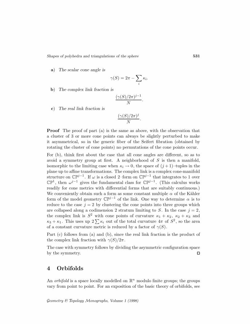
Shapes of polyhedra and triangulations of the sphere 531
a) The scalar cone angle is
γ(S) = 2π −∑
i
κi.
b) The complex link fraction is
(γ(S)/2π)j−1
N.
c) The real link fraction is
(γ(S)/2π)j
N.
Proof The proof of part (a) is the same as above, with the observation thata cluster of 3 or more cone points can always be slightly perturbed to makeit asymmetrical, so in the generic fiber of the Seifert fibration (obtained byrotating the cluster of cone points) no permutations of the cone points occur.
For (b), think first about the case that all cone angles are different, so as toavoid a symmetry group at first. A neighborhood of S is then a manifold,isomorphic to the limiting case when κi → 0, the space of (j + 1)–tuples in theplane up to affine transformations. The complex link is a complex cone-manifoldstructure on CPj−1 . If ω is a closed 2–form on CPj−1 that integrates to 1 overCP1 , then ωj−1 gives the fundamental class for CPj−1 . (This calculus worksreadily for cone metrics with differential forms that are suitably continuous.)We conveniently obtain such a form as some constant multiple α of the Kahlerform of the model geometry CPj−1 of the link. One way to determine α is toreduce to the case j = 2 by clustering the cone points into three groups whichare collapsed along a codimension 2 stratum limiting to S . In the case j = 2,the complex link is S2 with cone points of curvature κ1 + κ2 , κ2 + κ3 andκ3 + κ1 . This uses up 2
∑
κi out of the total curvature 4π of S2 , so the areaof a constant curvature metric is reduced by a factor of γ(S).
Part (c) follows from (a) and (b), since the real link fraction is the product ofthe complex link fraction with γ(S)/2π .
The case with symmetry follows by dividing the asymmetric configuration spaceby the symmetry.
4 Orbifolds
An orbifold is a space locally modelled on Rn modulo finite groups; the groupsvary from point to point. For an exposition of the basic theory of orbifolds, see
Geometry & Topology Monographs, Volume 1 (1998)

532 William P Thurston
[11]. Our orbifolds will be (X,G)–orbifolds, locally modelled on a homogeneousspace X with a Lie Group G of isometries. It is easily seen by inductionon dimension that an orientable (X,G)–orbifold has an induced metric whichmakes it into a cone-manifold. (Use the naturality of the exponential map.)
Here is a basic fact about the relation between cone-manifolds and orbifolds,which essentially is a rephrasing of Poincare’s theorem on fundamental domains:
Theorem 4.1 (Codimension 2 conditions suffice) Let C be an (X,G)–cone-manifold. Then C is a “weakening” of the structure of an orbifold if and onlyif all the codimension 2 strata of C have cone angles which that are integraldivisors of 2π .
Proof An orientation-preserving group of isometries whose fixed point set hascodimension 2 is a subgroup of SO(2), and the only possibilities are Z/n. Thecone angle along such a stratum in an orbifold is therefore an integral divisorof 2π , and the condition is necessary.
The converse can be proved by induction on the codimension of the singularstrata of C . Clearly, it works for strata of codimension 2. Suppose that wehave proven that C has an orbifold structure in the neighborhood of all strataup through codimension k . Let S be a singular stratum of codimension k + 1,and consider the neighborhood U of a point x ∈ S . This neighborhood can betaken to have the form of a bundle over a neighborhood of x in S , with fiberthe cone on a k–dimensional cone-manifold N , the normal sphere to S . Thenormal sphere N is modelled on (Sk, G), where G ⊂ SO(n). By induction,N is an orbifold; its universal cover must be Sk , since for k ≥ 2 the sphereis simply-connected. Therefore the cone on N is the quotient of Bk+1 by thegroup of covering transformations of Sk over N , and therefore U is also thequotient space of a neighborhood in X by the same group. Thus, C is anorbifold.
To illustrate, let’s look at some of the local orbifold structures that arise inmulti-way collisions. When k cone points of equal curvature 2πα collide, theorder of the local group Γ(S) for a stratum S is the reciprocal of the realvolume fraction, so from 3.6, setting α = γ(S)/2π we have
#Γ(S) =k!
(1 − kα)k−1
[
1
1/2 − α∈ Z & 0 < α < 1/k
]
The only three cases satisfying the condition for three colliding equal anglecone points are when α is 1/6, 1/4 and 3/10. The complex links in these
Geometry & Topology Monographs, Volume 1 (1998)

Shapes of polyhedra and triangulations of the sphere 533
three cases are the quotient orbifolds of the sphere by the oriented symmetriesof one of the regular polyhedra: (2, 3, 3), (2, 3, 4) or (2, 3, 5). The real link isS3 with a cone axis along the trefoil knot of order 3, 4 or 5. The formula givesorders for these groups of 24, 96 and 600. (This can be quickly confirmed by anautomated check using the 3–dimensional topology program Snappea to obtainpresentations for the orbifold fundamental groups and feeding then to a grouptheory program such as Magnus.)
An interesting example of a collision of cone points of unequal curvatures is(19π/30, 11π/30, 29π/30). The real link is an orbifold with (2, 3, 5) cone axeson the 3–component Hopf link. In this case, α = 1/60 and #(Γ(S)) = (60)2 =3600.
The biggest possible multiple collision is when 5 points of curvature π/3 collide.The local group for this collision has order 645! = 155, 520.
Infinitely many of the modular spaces for cone-metrics with 4 cone points areorbifolds of complex dimension 1, but for higher dimensional modular spaces,only 94 are orbifolds. These are tabulated in the appendix.
5 Proof of main theorem
Proof of Theorem 0.2 Most of this theorem follows formally from Theorem3.4, Proposition 3.5, and Theorem 4.1. What still remains is a discussion of thevolume of C(α1, . . . , αk).
The only case in which X = C(α1, . . . , αk) is not compact is where there arecone-manifolds x ∈ X whose diameters tend to infinity. In such a case, if wenormalize so that the area of x is 1, there must be subsets of x with largediameter and small area, free from cone points. This implies that x has subsetswhich are approximately isometric to a thin Euclidean cylinder. If γ ⊂ x isa short curve going around such an approximate cylinder, then the angle ofrotation for γ must be a sum of a subset of the {αi}. There are only a finitenumber of possibilities, so if the diameter is large enough, a neighborhood of γof large diameter is actually a cylinder. Once γ is determined, the shapes ofthe two pieces of x cut by γ can be specified independently, and a scale factorlength(γ)2/ area (less than some constant ǫ) together with an angle of rotationcan also be specified independently.
It will follow that the ends of x are in 1–1 correspondence with partitions Qof the set of curvatures into two subsets each summing to 2π , if we verify twopoints:
Geometry & Topology Monographs, Volume 1 (1998)

534 William P Thurston
(i) for any such partition Q, there exists an x ∈ X with a geodesic γ sepa-rating the cone points according to Q, and
(ii) the subspace Xγ,ǫ consisting of cone-manifolds in X with a geodesic γof length ǫ which separates the cone points according to Q is connected.
Actually, the proof does not logically depend on either point, and it is a slightdigression to prove them, but it seems worth doing anyway.
An easy demonstration of (i) is to construct a polygon with angles π−αi/2. Itis easy to find a very thin polygon realizing Q. Doubling such a polygon givesa suitable cone-manifold x.
We will describe an explicit construction for (ii). Let us begin with the specialcase of c ∈ Xγ,ǫ which are obtained by doubling a convex Euclidean polygonwhose angles are half the cone angles for X . It is easy to connect any two convexpolygons with the same sequence of angles by a family of polygons having thesame angles. If we allow degenerate cases as well, where two angles coincide,the order is irrelevant. Therefore, this special subspace of Xγ,ǫ is connected.
Therefore, it suffices to connect any c ∈ Xγ,ǫ to something obtained by doublinga convex polygon. Construct a maximal cylindrical neighborhood N1 of γwith geodesic boundary. There is at least one cone point on each boundarycomponent of N1 . Let β be one of the boundary components, and x1 ∈ β acone point, with curvature α. If c is cut along β , the portion on the other sideof β from N1 has boundary consisting of a geodesic with a convex angle of π−αat x1 , and possibly additional angles if it contains other cone points. There isa circular arc β′ through x1 , contained in N , which appears to have a convexangle of π − α from within N , but appears to be smooth at x1 when viewedfrom the outside. Let U1 be the “outside” component obtained by cutting alongβ′ . Its boundary is now locally isometric to a circle, and a neighborhood, likeon a cone, is foliated by parallel circles.
Deform c, by shrinking the “interesting part” of U1 relative to the rest of c,so that the next cone point in U1 is not close to β′ . Let N2 be a maximalneighborhood of β′ which is foliated by parallel circles, and let x2 be a pointon its boundary. Adjust by a rotation of U1 until the geodesic through x1
perpendicular to the foliation by circles hits at x2 . Draw a circular arc throughx2 , within U1 , which appears smooth from the outside neighborhood U2 .
This process can be continued, in the same manner, until the last neighborhoodUk is a cone. The geodesic through xk−1 automatically hits the cone point. Nowdo the same process on the other side of N1 , first adjusting by a rotation so a
Geometry & Topology Monographs, Volume 1 (1998)
Shapes of polyhedra and triangulations of the sphere 535
geodesic through x1 perpendicular to the foliation of N1 by parallel circles hitsat a cone point.
After this sequence of deformations, we have a cone-manifold with a geodesicHamiltonian path through all the cone points, such that at cone points internalto it the two outgoing geodesics bisect the cone angle. The path can be com-pleted to a curve by one additional geodesic (this is easy to see if you draw thefigure in the plane obtained by cutting along the path; it is made of two convexarcs, and has bilateral symmetry).
Note that a similar process works for a general cone-manifold: we do not reallyneed γ for this construction, we can begin at any cone point, and work outwardfrom it.
We call the ends of X cusps, in accordance with terminology for manifoldsand orbifolds. To justify this word, note that each cusp is foliated by complexgeodesics with respect to the Hermitian metric, obtained by rotating the twoends of c with respect to each other and by scaling. The complex geodesicsare locally isometric to the hyperbolic plane. The pure scaling, which may bethought of as inserting extra lengths of cylinder between the two ends, generatesa real geodesic. These real geodesics converge, as the shrinking increases. Theconvergence is exponential, so the total volume of each cusp is finite.
6 The icosahedron and other polyhedra
Let A be the subgroup of isometries of C which take Eis into itself. We maythink of the classes of triangulations P (n; k1, . . . , km) as the space of (E2, A)–cone-manifolds of area n (measured in double triangles) and cone angles kiπ/3.They consist of elements of C(k1π/3, . . . , knπ/3) equipped with a reduction ofthe (E2, isom(E2)) structure to (E2, A). In more concrete terms, a triangulationis given by a cocycle whose coefficients are elements of Eis.
Euclidean cone-manifolds sometimes admit several inequivalent reductions to(E2, A)—in other words, there are some cone-manifolds that can be subdividedinto unit equilateral triangles in more than one way. In complex Lorentz spaceC(m−3,1) , the set of cocyles with a certain total area form a sheet of a hy-perboloid. The hyperboloid fibers over complex hyperbolic space, with fiber acircle (corresponding to multiplication of the cocycle by elements of the unitcircle). The set of triangulations are lattice points in C(m−3,1) , and the value ofthe Hermitian form counts the number of triangles—multiple unit equilateraltriangulations of a Euclidean manifold correspond to fibers that intersect more
Geometry & Topology Monographs, Volume 1 (1998)

536 William P Thurston
than lattice points. (All lattice points come in groups of 6 whose ratios areunits in the ring Eis.)
Figure 12: If an icosahedron is slit along 6 disjoint arcsjoining its vertices in pairs, conical caps can be insertedto turn it into an octahedron.
The “biggest” of the classes of triangulations is
P (n; 1, 1, . . . , 1) ⊂ J = C(π/3, π/3, . . . , π/3),
the one which contains the icosahedraon. The “completion” P (n; 1, . . . , 1) ⊂ Jwhich includes degenerate cases contains all the other classes of triangulations.
By theorem 1.2, J is a complex hyperbolic orbifold of dimension 9. The coneangles around the complex codimension 1 singular strata are 2π/3.
There is a concrete construction to describe an arbitrary element of J or ofP (1, . . . , 1), as follows. Suppose first that x ∈ J is an arbitrary Euclideancone-metric on the sphere with all cone points having curvature π/3. Choosea collection of 6 disjoint geodesic arcs with endpoints on the cone points. Slitalong each of these arcs.
Locally near the endpoints of the arcs, the developing map maps the slit surfaceto the complement of a 60◦ angle. A neighborhood of the slit develops to aregion outside an equilateral triangle in the plane; when you go once aroundthe slit, the developing image goes 2/3 of the way around the triangle.
For each slit, take 2/3 of an equilateral triangle with side equal to the length ofthe slit, fold it together to form a cone point in the center of the original trianglewith curvature 2π/3 and glue it into the slit. The result is a cone-manifold f(x)like the octahedron, in C(2π/3, 2π/3, 2π/3, 2π/3, 2π/3, 2π/3).
As in section 2, we can analyze the shape of f(x) by joining its cone pointsin pairs by disjoint geodesic segments, slitting open, and extending to give anelement of C(4π/3, 4π/3, 4π/3) (which is a single point).
If x ∈ J − J , the analysis still works: treat the cone points as cone points withmultiplicity, and use zero-length slits as much as possible at cone points withcurvature greater than π/3. At the first step, the slits of positive length pairthe cone points with curvature an odd multiple of π/3. When the slits are filled
Geometry & Topology Monographs, Volume 1 (1998)
Shapes of polyhedra and triangulations of the sphere 537
in, the curvature at each of the endpoints is decreased by π/3, and the resultingcone-manifold has all curvatures an even multiple of π/3. For the second step,note that no cone point can have curvature 6π/3 or bigger. In this case, theslits of positive length join cone points with curvature 2π/3.
An arbitrary x ∈ J can be reconstructed by reversing this procedure.
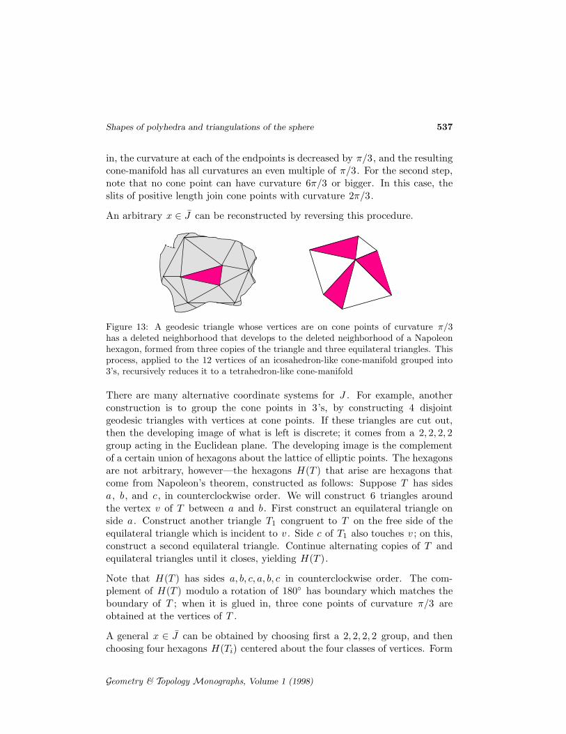
Figure 13: A geodesic triangle whose vertices are on cone points of curvature π/3has a deleted neighborhood that develops to the deleted neighborhood of a Napoleonhexagon, formed from three copies of the triangle and three equilateral triangles. Thisprocess, applied to the 12 vertices of an icosahedron-like cone-manifold grouped into3’s, recursively reduces it to a tetrahedron-like cone-manifold
There are many alternative coordinate systems for J . For example, anotherconstruction is to group the cone points in 3’s, by constructing 4 disjointgeodesic triangles with vertices at cone points. If these triangles are cut out,then the developing image of what is left is discrete; it comes from a 2, 2, 2, 2group acting in the Euclidean plane. The developing image is the complementof a certain union of hexagons about the lattice of elliptic points. The hexagonsare not arbitrary, however—the hexagons H(T ) that arise are hexagons thatcome from Napoleon’s theorem, constructed as follows: Suppose T has sidesa, b, and c, in counterclockwise order. We will construct 6 triangles aroundthe vertex v of T between a and b. First construct an equilateral triangle onside a. Construct another triangle T1 congruent to T on the free side of theequilateral triangle which is incident to v . Side c of T1 also touches v ; on this,construct a second equilateral triangle. Continue alternating copies of T andequilateral triangles until it closes, yielding H(T ).
Note that H(T ) has sides a, b, c, a, b, c in counterclockwise order. The com-plement of H(T ) modulo a rotation of 180◦ has boundary which matches theboundary of T ; when it is glued in, three cone points of curvature π/3 areobtained at the vertices of T .
A general x ∈ J can be obtained by choosing first a 2, 2, 2, 2 group, and thenchoosing four hexagons H(Ti) centered about the four classes of vertices. Form
Geometry & Topology Monographs, Volume 1 (1998)
538 William P Thurston
the quotient of the complement of the hexagons by the group, and glue in thetriangles Ti . If the hexagons are disjoint and nondegenerate, x ∈ J .
From this concrete point of view, what is amazing is that these coordinatesystems have a global meaning, since J is an orbifold: even if one chooses acollection of hexagons H(Ti) which overlap, they determine a unique Euclideancone-manifold, provided the net area (computed formally) is positive.
Using these constructions, it is not hard to show that P (n; 1, . . . , 1) contains1 or more elements for all values of n starting with 10, with 11 as the soleexception. If there were an element T of P (11, 1, . . . , 1), it would have 13vertices and 22 triangles. One could then construct a spherical cone-manifoldby using equilateral spherical triangles with angles 2π/5. This cone-manifoldwould have only one cone point — which is manifestly impossible, since theholonomy for a curve going around the cone point is a rotation of order 5, butat the same time the holonomy is trivial since the curve is the boundary of adisk having a spherical structure.
From the picture in C(1,9) , it follows that the number of non-negatively curvedtriangulations having up to 2n triangles is roughly proportional to the volumeof the intersection of some cone with the ball of radius
√n in this indefinite
metric. The cone in question is neither compact nor convex, but since it comesfrom a fundamental domain for the group action, its intersection with the ball ofnorm less than any constant has finite 10–real-dimensional volume. Therefore,the number of triangulations with up to 2n triangles is O(n10).
7 An explicit construction and fundamental domain
Another method for constructing, manipulating and analyzing non-negativelycurved cone structures goes as follows:
Given k + 1 real numbers α0, α1, . . . , αk ≥ 0 whose sum is 4π .
To Construct Euclidean cone-metrics with the αi as curvatures.
Choose a k–gon P in the plane, with edges e1 . . . , ek .
Construct (i = 1, . . . k): An isosceles triangles Ti with base on ei , apex vi ,apex angle αi , pointing inward if αi < π , pointing outward if αi > π .
Condition A the triangles Ti are disjoint from each other and disjoint fromP except along ei .
Let Q be thefilled polygon obtained from P by replacing each ei by the othertwo sides fi and gi of Ti .
Geometry & Topology Monographs, Volume 1 (1998)

Shapes of polyhedra and triangulations of the sphere 539
Glue fi to gi to obtain a cone manifold. The vertex vi becomes a cone pointof curvature αi . The other k vertices of P all join to form a cone pointof cone angle α0 .
Figure 14: A cube-like cone-metric (8 cone-angles of curvature π/2) can be constructedby removing isosceles right triangles from the sides of a heptagon and gluing the result-ing pairs of equal sides. The seven sharp angles all come together to form the eigth conepoint. This illustration (along with the others in this section) was constructed withthe program Geometer’s Sketchpad , where the shape can be varied while preservingthe correct geometric relations.
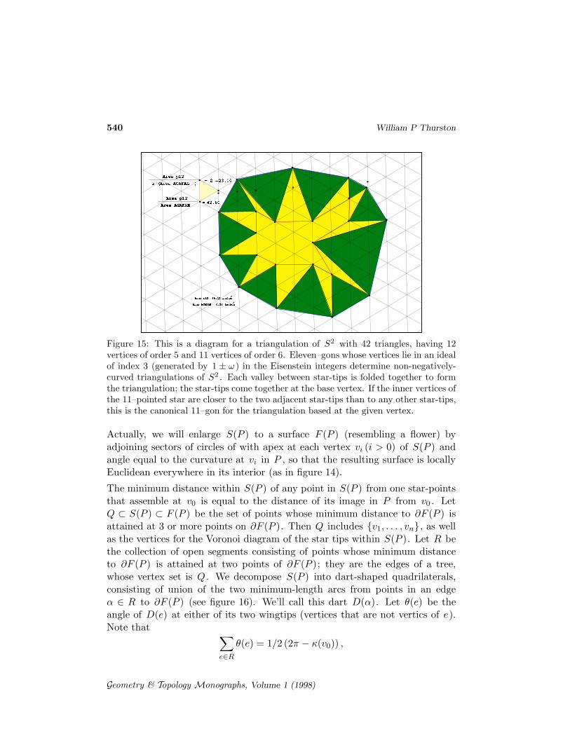
As examples, see figure 14 for a cube-like cone-manifold, or figure 15 for a trian-gulation of S2 with 23 vertices and 42 triangles constructed from an icosahedral-like cone-manifold.
Here is the inverse construction. Given a cone-metric with n cone points onS2 :
Choose one of the cone points v0 .
Find for each other cone point vi a shortest path ai from v0 to vi . The ai
are necessarily simple and disjoint, except at v0 .
Cut along all these paths, to obtain a disk equipped with a Euclidean metricwhose boundary is composed of 2(n − 1) straight segments, each pairedto an adjacent segment of the same length and forming an angle equal tothe corresponding cone angle. (See figure 16.)
We will show that if P is a cone-metric on the sphere with positive curvatureat each vertex, and if S(P ) (S because it resembles a star) is the metric onD2 obtained by cutting P open as above, then S(P ) can be flattened outinto the plane, that is, it is isometric to the metric of a filled simple polygon.
Geometry & Topology Monographs, Volume 1 (1998)
540 William P Thurston
Figure 15: This is a diagram for a triangulation of S2 with 42 triangles, having 12vertices of order 5 and 11 vertices of order 6. Eleven–gons whose vertices lie in an idealof index 3 (generated by 1 ± ω ) in the Eisenstein integers determine non-negatively-curved triangulations of S2 . Each valley between star-tips is folded together to formthe triangulation; the star-tips come together at the base vertex. If the inner vertices ofthe 11–pointed star are closer to the two adjacent star-tips than to any other star-tips,this is the canonical 11–gon for the triangulation based at the given vertex.
Actually, we will enlarge S(P ) to a surface F (P ) (resembling a flower) byadjoining sectors of circles of with apex at each vertex vi (i > 0) of S(P ) andangle equal to the curvature at vi in P , so that the resulting surface is locallyEuclidean everywhere in its interior (as in figure 14).
The minimum distance within S(P ) of any point in S(P ) from one star-pointsthat assemble at v0 is equal to the distance of its image in P from v0 . LetQ ⊂ S(P ) ⊂ F (P ) be the set of points whose minimum distance to ∂F (P ) isattained at 3 or more points on ∂F (P ). Then Q includes {v1, . . . , vn}, as wellas the vertices for the Voronoi diagram of the star tips within S(P ). Let R bethe collection of open segments consisting of points whose minimum distanceto ∂F (P ) is attained at two points of ∂F (P ); they are the edges of a tree,whose vertex set is Q. We decompose S(P ) into dart-shaped quadrilaterals,consisting of union of the two minimum-length arcs from points in an edgeα ∈ R to ∂F (P ) (see figure 16). We’ll call this dart D(α). Let θ(e) be theangle of D(e) at either of its two wingtips (vertices that are not vertics of e).Note that
∑
e∈R
θ(e) = 1/2 (2π − κ(v0)) ,
Geometry & Topology Monographs, Volume 1 (1998)
Shapes of polyhedra and triangulations of the sphere 541
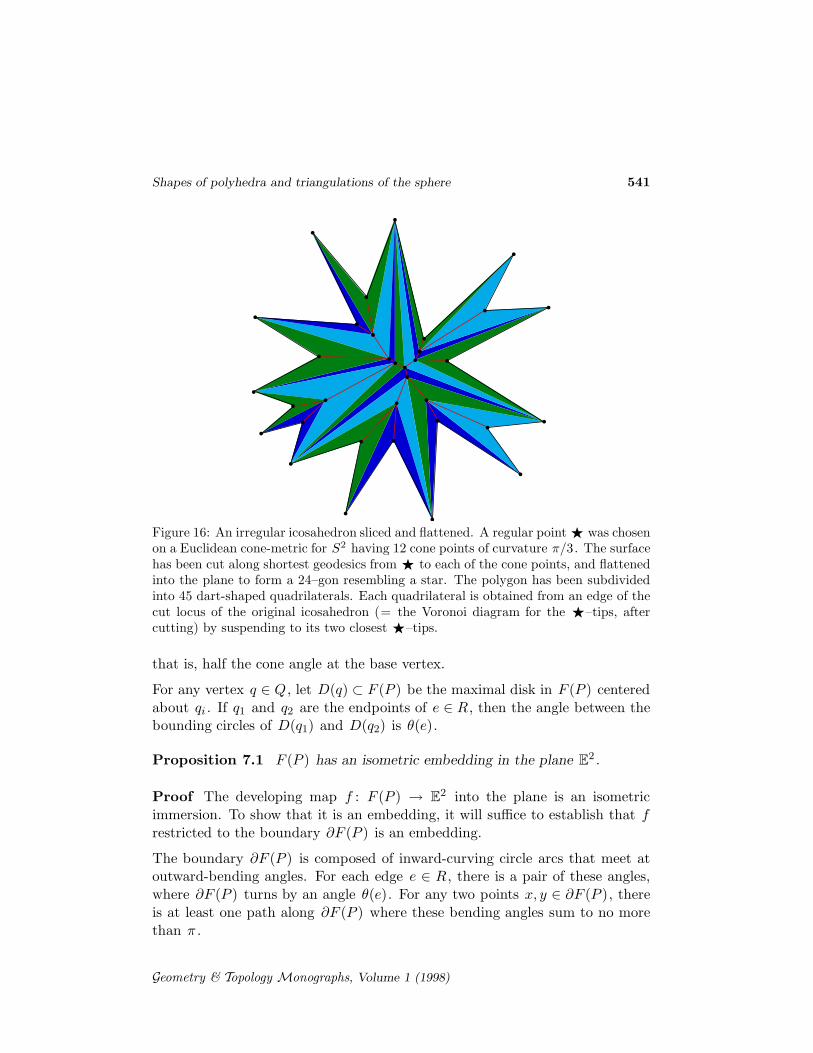
Figure 16: An irregular icosahedron sliced and flattened. A regular point ⋆ was chosenon a Euclidean cone-metric for S2 having 12 cone points of curvature π/3. The surfacehas been cut along shortest geodesics from ⋆ to each of the cone points, and flattenedinto the plane to form a 24–gon resembling a star. The polygon has been subdividedinto 45 dart-shaped quadrilaterals. Each quadrilateral is obtained from an edge of thecut locus of the original icosahedron (= the Voronoi diagram for the ⋆–tips, aftercutting) by suspending to its two closest ⋆–tips.
that is, half the cone angle at the base vertex.
For any vertex q ∈ Q, let D(q) ⊂ F (P ) be the maximal disk in F (P ) centeredabout qi . If q1 and q2 are the endpoints of e ∈ R, then the angle between thebounding circles of D(q1) and D(q2) is θ(e).
Proposition 7.1 F (P ) has an isometric embedding in the plane E2 .
Proof The developing map f : F (P ) → E2 into the plane is an isometricimmersion. To show that it is an embedding, it will suffice to establish that frestricted to the boundary ∂F (P ) is an embedding.
The boundary ∂F (P ) is composed of inward-curving circle arcs that meet atoutward-bending angles. For each edge e ∈ R, there is a pair of these angles,where ∂F (P ) turns by an angle θ(e). For any two points x, y ∈ ∂F (P ), thereis at least one path along ∂F (P ) where these bending angles sum to no morethan π .
Geometry & Topology Monographs, Volume 1 (1998)
542 William P Thurston
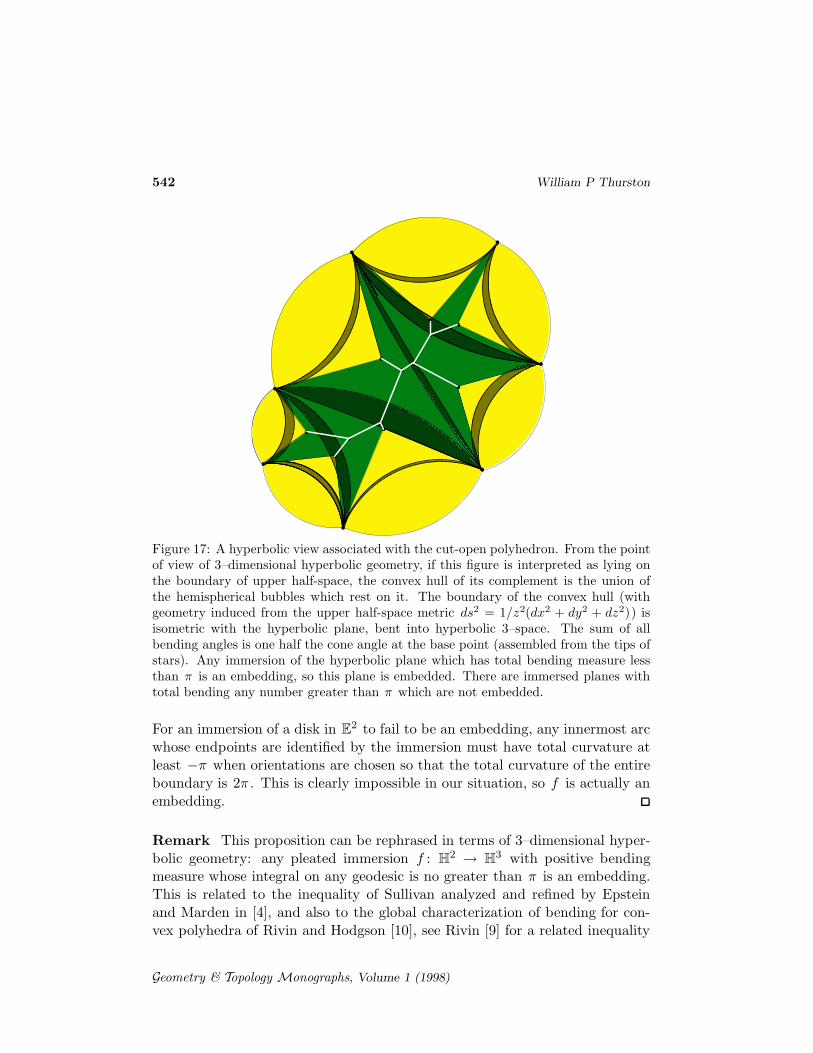
Figure 17: A hyperbolic view associated with the cut-open polyhedron. From the pointof view of 3–dimensional hyperbolic geometry, if this figure is interpreted as lying onthe boundary of upper half-space, the convex hull of its complement is the union ofthe hemispherical bubbles which rest on it. The boundary of the convex hull (withgeometry induced from the upper half-space metric ds2 = 1/z2(dx2 + dy2 + dz2)) isisometric with the hyperbolic plane, bent into hyperbolic 3–space. The sum of allbending angles is one half the cone angle at the base point (assembled from the tips ofstars). Any immersion of the hyperbolic plane which has total bending measure lessthan π is an embedding, so this plane is embedded. There are immersed planes withtotal bending any number greater than π which are not embedded.
For an immersion of a disk in E2 to fail to be an embedding, any innermost arcwhose endpoints are identified by the immersion must have total curvature atleast −π when orientations are chosen so that the total curvature of the entireboundary is 2π . This is clearly impossible in our situation, so f is actually anembedding.
Remark This proposition can be rephrased in terms of 3–dimensional hyper-bolic geometry: any pleated immersion f : H2 → H3 with positive bendingmeasure whose integral on any geodesic is no greater than π is an embedding.This is related to the inequality of Sullivan analyzed and refined by Epsteinand Marden in [4], and also to the global characterization of bending for con-vex polyhedra of Rivin and Hodgson [10], see Rivin [9] for a related inequality
Geometry & Topology Monographs, Volume 1 (1998)

Shapes of polyhedra and triangulations of the sphere 543
for convex hyperbolic polyhedra.
The n–dimensional associahedron is a polyhedron whose vertices are labelled bytriangulations of an (n + 3)–gon using only vertices of the polygon, and whosek–cells are labelled by subdivisions of the (n + 3)–gon obtained by removing kedges from a triangulation. They can be thought of as describing all ways toparenthesize or associate a product of n + 2 symbols. The associahedron is aconvex polyhedron in n–space that arises in a variety of mathematical contextincluding the theory of loop spaces, Teichmuller theory and numerous combi-natorial settings. The numbers of triangulations are called Catalan numbers.
If cone angles at the n points of P are fixed, the angles θ(e) that can occur forour dart quadrilaterals can be described by mapping the n−1 star tips of S(P )to the vertices of a regular (n− 1)–gon, mapping each dart quadrilateral D(e)to an edge or a chord of this polygon, and labelling each edge by the angle θ(e).(In terms of hyperbolic geometry, this is an element of the measured laminationspace for the ideal polygonal orbifold (∞,∞, . . . ,∞).) This determines a pointin a polyhedron Fn closely related to an associahedron, namely, the join of theboundary of the dual of the (n−4)–dimensional associahedron with the (n−2)–simplex. (When the measure on the boundary of the polygon is zero, we get apoint on the boundary of the dual of the (n − 4)–dimensional associahedron.Measures on the polygon itself with fixed total weight form an (n−2)–simplex.)
The set of all possible functions θ(e) (which we refer to as measures, after theusage in hyperbolic geometry and Teichmuller theory) can be described globallyas a convex polyhedron using dual train track coordinates, as follows: rotatea copy of the regular (n − 1)–gon 1/(2n − 2)th of a revolution so it is out ofphase with itself. Choose any triangulation of this rotated polygon, using onlyits vertices. For each edge f of this triangulation, let m(f) be the sum of θ(e)where e intersects f . For any triangle with sides f, g, h, the quantities m(f),m(g) and m(h) satisfy the three triangle inequalities m(f)+m(g) ≥ m(h) etc.These measures are subject to one linear constraint, namely, the sum of m(f)where f ranges over the edges of the rotated polygon adds to the cone angle atthe base vertex v0 .
For any set of numbers {m(f)} satisfying the linear equation and linear in-equalities, a measured lamination having total measure π − α0/2, where α0 isthe cone angle at v0 , can be reconstructed by a simple method familiar in thetheory of measured foliations or normal curves on surfaces, by first solving forthe picture in each triangle of the rotated polygon, then gluing the trianglestogether. From this measured lamination and from the specification of coneangles (in order) at v1, . . . vn−1 , a star polygon in the plane can be constructed
Geometry & Topology Monographs, Volume 1 (1998)

544 William P Thurston
recursively, using the principle that the shape of any dart quadrilateral D(e)is determined from θ(e) together with either of its other two angles. This starpolygon is determined up to similarity. When glued together it forms a conemanifold with specified cone-angles.
If all cone angles are equal, and if we are not distinguishing shapes that arethe same up to permutation of the labels of cone points v1, . . . vn−1 , then wemust divide F by action of the group of order n − 1 rotations. The faces ofF correspond to measures θ where one of the edges of the (n − 1)–gon hasmeasure 0. Geometrically, this means that one of the cone points vi , i > 0 hastwo or more shortest paths on P to v0 . We could cut P open along either ofthese shortest paths. In S(P ), this means one of the “inside” vertices of thestar has three or more shortest paths to the tip vertices: two are sides of S(P ),and at least one is interior to S(P ). You can cut S(P ) along such an edge,and rotate one resulting chunk with respect to the other, to obtain a new shapeS′(P ) with vertices in a permuted order.
To also insist on allowing change of base point requires a further much less directequivalence relation. If the cone angles α1, . . . , αn−1 are not all the same, thento get all possible cone-metrics, we need one copy of F for each ordering of thecone angles up to cyclic permutation.
8 Teichmuller space interpretation
Each element of C(α1, . . . , αn) determines a point in a certain finite sheetedcovering of the modular orbifold for the n–punctured sphere. (The coveringcorresponds to the subgroup of the modular group for the n–punctured spherewhich preserves the cone angles): the map consists of forgetting the metric, andremembering only the conformal structure.
By the uniformization theorem, each of these metrics is equivalent to a metricobtained by deleting n points from the Riemann sphere C. The resultingconfiguration of n points in C is unique up to Mobius transformations.
Proposition 8.1 The map from C(α1, . . . , αn) is a homeomorphism.
Proof In fact, there is an explicit formula for the inverse map, going from aconfiguration of n points on C together with the curvatures at those pointsto a Euclidean cone-manifold with the given conformal structure. The formulais essentially the same as the Schwarz–Christoffel formula for uniformizing a
Geometry & Topology Monographs, Volume 1 (1998)

Shapes of polyhedra and triangulations of the sphere 545
rectilinear polygon. (See [12] for an analysis of these and other cone-manifoldstructures.)
The idea is to think of the construction of a Euclidean cone metric on C interms of its developing map h. Consider a collection {yi} of points in C, withdesired curvatures {αi}. Let P be the punctured Riemann sphere C−{yi}. Thedeveloping map h is not uniquely determined on P , and it is only defined on theuniversal cover P , but any two choices differ by a complex affine transformation.Therefore, the pre-Schwarzian of h, that is, S = h′′/h′ , is uniquely determinedby the metric, and it is defined on P , not just on the universal cover of P .The Euclidean metric can be easily reconstructed if we are given S , becauseonce we choose an initial value and derivative for the developing map h at onepoint on P , we can integrate the differential equation h′′ = Sh′ to determineit everywhere else.
How can we determine S? Consider a cone, with curvature α at the its apex.If a cone is conformally mapped to C with its apex going to the origin, thedeveloping map is z 7→ z1− α
2π . The pre-Schwarzian for this map is − α2π
z−1 . Itfollows that the pre-Schwarzian for the developing map of any Euclidean cone-metric with a cone point having curvature α will have a pole at the cone point,with residue − α
2πz−1 . Conversely, if the pre-Schwarzian of some function h has
a pole of this type at any point in C, then h will locally be the developingmap for a Euclidean structure with a cone point of angle α. (To see this,observe that the analytic continuation of h around the pole differs by post-composition with an affine transformation. Using this information, one canmake a local conformal change of coordinates in the domain so that h has theform z 7→ z1− α
2π , where α is not necessarily real. From this, one sees that thepre-Schwarzian has a pole at the singularity with residue α/2π .)
We may as well assume that the the {yi} are in the finite part of C. Define
S =∑
i
− α
2π(z − y−1).
Computation shows that in a coordinate patch w = z−1 for a neighborhood of∞, the pre-Schwarzian in terms of the variable w is holomorphic if and onlyif S behaves asymptotically like −2z−1 . This is satisfied in our case, since thesum of the αi is 4π . The condition that S is holomorphic on P , and that ithas the given behaviour at the cone points and at ∞, uniquely determines S .
S determines a complex affine structure on P . Since the fundamental groupof P is generated by loops going around the punctures, and since the holon-omy around these loops is isometric, the affine structure is compatible with aEuclidean structure, well-defined up to scaling.
Geometry & Topology Monographs, Volume 1 (1998)
546 William P Thurston
Thus, we may think of C(α1, . . . , αn) as a certain geometric interpretation ofmodular space. The completions C(α1, . . . , αn) have a topology which dependson the comparisons of sums of subsets of the αi with 2π . It is almost neveragrees with the standard compactification of the modular space. However, thereare only a finite number of possible possibilities for the topology — it is curiousthat we thus obtain several parameter families of complex hyperbolic structureson the Teichmuller space, and several parameter families of complex hyperboliccone-manifolds on the various C(α1, . . . , αn), with varying cone angles.
Is there any similar phenomenon for the Teichmuller spaces of other surfaces,particularly closed surfaces? The surface of genus 2 has the same modularspace as the six–punctured sphere, so for that particular case, the constructioncarries over. I don’t know how to extend it to surfaces of higher genus.
References
[1] D Cooper, WP Thurston, Triangulating 3–manifolds using 5 vertex links,Topology, 27 (1988) 23–25
[2] P Deligne, G D Mostow, Monodromy of hypergeometric functions and non-
lattice integral monodromy, Inst. Hautes Etudes Sci. Publ. Math. 63 (1986) 5–89
[3] P Deligne, G D Mostow, Commensurabilities among lattices in PU(1, n),Annals of Mathematics Studies, 132, Princeton University Press, Princeton, NJ(1993)
[4] DB A Epstein, A Marden, Convex hulls in hyperbolic space, a theorem of
Sullivan, and measured pleated surfaces, from: “Analytical and geometric as-pects of hyperbolic space (Coventry/Durham, 1984)”, Cambridge Univ. Press,Cambridge (1987) 113–253
[5] G D Mostow, Generalized Picard lattices arising from half-integral conditions
Inst. Hautes Etudes Sci. Publ. Math. 63 (1986) 91–106
[6] E Picard, Sur les fonctions hyperfuchsiennes provenant des series hy-
pergeometriques de deux variables, Ann. ENS III, 2 (1885) 357–384
[7] E Picard, Sur une extension aux fonctions de deux variables du probleme de
Riemann relatif aux fonctions hypergeometriques, Bull. Soc. Math. Fr. 15 (1887)148–152
[8] Igor Rivin, Euclidean structures on simplicial surfaces and hyperbolic volume,Annals of Math. 139 (1994) 553–580
[9] Igor Rivin, A characterization of ideal polyhedra in hyperbolic 3–space, Annalsof Math. 143 (1996) 51–70
[10] Igor Rivin, Craig D Hodgson, A characterization of compact convex poly-
hedra in hyperbolic 3–space, Invent. Math. 111 (1993) 77–111
Geometry & Topology Monographs, Volume 1 (1998)

Shapes of polyhedra and triangulations of the sphere 547
[11] William P Thurston, Geometry and Topology of Three–Manifolds, Princetonlecture notes (1979) http://www.msri.org/publications/books/gt3m
[12] Marc Troyanov, Prescribing curvature on compact surfaces with conical sin-
gularities, Trans. Amer. Math. Soc. 324 (1991) 793–821
Mathematics DepartmentUniversity of California at DavisDavis, CA 95616, USA
Email: [email protected]
Received: 15 November 1997 Revised: 27 November 1998
Appendix: 94 orbifolds
We give below a list of the examples of the spaces C(α1, . . . , αn) which are orbifolds,for n ≥ 5. When n = 3 there is only one example for each feasible triple of cone angles,and for n = 4 there are infinitely many examples. In fact, every triangle group in thehyperbolic plane can be interpreted as the modular space for families of tetrahedra. Ingeneral, the αi are of the form 2πp
q, for p and q integers. For each example, we list the
least denominator q and the sequence of numerators pi . We also list the degree of thenumber field containing the roots of unity exp(2πpi
q) (that is, the number of integers
less than q relatively prime to q ). We list also three additional bits of information:
(arithmetic) Is the orbifold arithmetic (AR) or non-arithmetic (NR)?
(pure) Is the completion of the covering of the modular space whose fundamentalgroup is the pure braid group an orbifold (P), or are some interchanges of pairsof cone points needed to make the orbifold (I)?
(compact) Is the orbifold compact (C) or non-compact (N)?
The question of arithmeticity hinges on the signatures of the Hermitian forms obtainedwhen we conjugate the curvatures at the cone points (considered as roots of unity) bythe Galois automorphisms. If all the other signatures are negative definite or positivedefinite, the group is arithmetic; otherwise not. The other two questions are moreobvious.
These examples were enumerated by a routine computer program, which checks allpossibilities having a given least common denominator q . The enumeration was notrigorously verified (even though it should not be hard to do so and search more ‘intelli-gently’ at the same time) but was a simple check of all denominators through 999 in afew minutes of computer time. Mostow has rigorously enumerated examples by hand,so this table can be regarded as just a check.
Geometry & Topology Monographs, Volume 1 (1998)
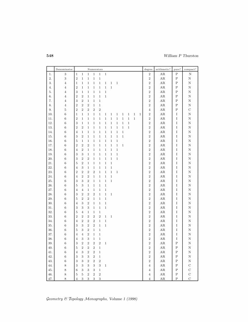
548 William P Thurston
Denominator Numerators degree arithmetic? pure? compact?
1. 3 1 1 1 1 1 1 2 AR P N
2. 3 2 1 1 1 1 2 AR P N
3. 4 1 1 1 1 1 1 1 1 2 AR P N
4. 4 2 1 1 1 1 1 1 2 AR P N
5. 4 3 1 1 1 1 1 2 AR P N
6. 4 2 2 1 1 1 1 2 AR P N
7. 4 3 2 1 1 1 2 AR P N
8. 4 2 2 2 1 1 2 AR P N
9. 5 2 2 2 2 2 4 AR P C
10. 6 1 1 1 1 1 1 1 1 1 1 1 1 2 AR I N
11. 6 2 1 1 1 1 1 1 1 1 1 1 2 AR I N
12. 6 3 1 1 1 1 1 1 1 1 1 2 AR I N
13. 6 2 2 1 1 1 1 1 1 1 1 2 AR I N
14. 6 4 1 1 1 1 1 1 1 1 2 AR I N
15. 6 3 2 1 1 1 1 1 1 1 2 AR I N
16. 6 5 1 1 1 1 1 1 1 2 AR I N
17. 6 2 2 2 1 1 1 1 1 1 2 AR I N
18. 6 4 2 1 1 1 1 1 1 2 AR I N
19. 6 3 3 1 1 1 1 1 1 2 AR I N
20. 6 3 2 2 1 1 1 1 1 2 AR I N
21. 6 5 2 1 1 1 1 1 2 AR I N
22. 6 4 3 1 1 1 1 1 2 AR I N
23. 6 2 2 2 2 1 1 1 1 2 AR I N
24. 6 4 2 2 1 1 1 1 2 AR I N
25. 6 3 3 2 1 1 1 1 2 AR I N
26. 6 5 3 1 1 1 1 2 AR I N
27. 6 4 4 1 1 1 1 2 AR I N
28. 6 3 2 2 2 1 1 1 2 AR I N
29. 6 5 2 2 1 1 1 2 AR I N
30. 6 4 3 2 1 1 1 2 AR I N
31. 6 3 3 3 1 1 1 2 AR I N
32. 6 5 4 1 1 1 2 AR I N
33. 6 2 2 2 2 2 1 1 2 AR I N
34. 6 4 2 2 2 1 1 2 AR I N
35. 6 3 3 2 2 1 1 2 AR I N
36. 6 5 3 2 1 1 2 AR I N
37. 6 4 4 2 1 1 2 AR I N
38. 6 4 3 3 1 1 2 AR I N
39. 6 3 2 2 2 2 1 2 AR P N
40. 6 5 2 2 2 1 2 AR P N
41. 6 4 3 2 2 1 2 AR P N
42. 6 3 3 3 2 1 2 AR P N
43. 6 3 3 2 2 2 2 AR P N
44. 8 3 3 3 3 3 1 4 AR P C
45. 8 6 3 3 3 1 4 AR P C
46. 8 5 5 2 2 2 4 AR P C
47. 8 4 3 3 3 3 4 AR P C
Geometry & Topology Monographs, Volume 1 (1998)
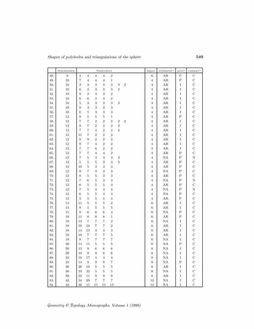
Shapes of polyhedra and triangulations of the sphere 549
Denominator Numerators degree arithmetic? pure? compact?
48. 9 4 4 4 4 2 6 AR P C
49. 10 7 4 4 4 1 4 AR P C
50. 10 3 3 3 3 3 3 2 4 AR I C
51. 10 6 3 3 3 3 2 4 AR I C
52. 10 9 3 3 3 2 4 AR I C
53. 10 6 6 3 3 2 4 AR I C
54. 10 5 3 3 3 3 3 4 AR I C
55. 10 8 3 3 3 3 4 AR I C
56. 10 6 5 3 3 3 4 AR I C
57. 12 8 5 5 5 1 4 AR P C
58. 12 7 7 2 2 2 2 2 4 AR I C
59. 12 9 7 2 2 2 2 4 AR I C
60. 12 7 7 4 2 2 2 4 AR I C
61. 12 11 7 2 2 2 4 AR I C
62. 12 9 9 2 2 2 4 AR I C
63. 12 9 7 4 2 2 4 AR I C
64. 12 7 7 6 2 2 4 AR I C
65. 12 7 7 4 4 2 4 AR P C
66. 12 7 5 3 3 3 3 4 NA P N
67. 12 5 5 5 3 3 3 4 AR P C
68. 12 10 5 3 3 3 4 AR P C
69. 12 8 7 3 3 3 4 NA P C
70. 12 8 5 5 3 3 4 AR P C
71. 12 7 6 5 3 3 4 NA P N
72. 12 6 5 5 5 3 4 AR P C
73. 12 7 5 4 4 4 4 NA P N
74. 12 6 5 5 4 4 4 NA P C
75. 12 5 5 5 5 4 4 AR P C
76. 14 11 5 5 5 2 6 AR I C
77. 14 8 5 5 5 5 6 AR I C
78. 15 8 6 6 6 4 8 NA P C
79. 18 11 8 8 8 1 6 AR P C
80. 18 13 7 7 7 2 6 NA I C
81. 18 10 10 7 7 2 6 AR I C
82. 18 14 13 3 3 3 6 AR I C
83. 18 10 7 7 7 5 6 AR I C
84. 18 8 7 7 7 7 6 NA I C
85. 20 14 11 5 5 5 8 NA P C
86. 20 13 9 6 6 6 8 NA I C
87. 20 10 9 9 6 6 8 NA I C
88. 24 19 17 4 4 4 8 NA I C
89. 24 14 9 9 9 7 8 NA P C
90. 30 26 19 5 5 5 8 AR I C
91. 30 23 22 5 5 5 8 NA I C
92. 30 22 11 9 9 9 8 AR I C
93. 42 34 29 7 7 7 12 NA I C
94. 42 26 15 15 15 13 12 NA I C
Geometry & Topology Monographs, Volume 1 (1998)
