shield tunnel
TRANSCRIPT
STUDY ON MECHANICAL BEHAVIOR AND
DESIGN OF COMPOSITE SEGMENT
FOR SHIELD TUNNEL
合成セグメントの力学的挙動および設計
法に関する研究
October 2009
Civil and Environmental Engineering
Graduate School of Science and Engineering
WASEDA University
早稲田大学大学院理工学研究科建設工学専攻
WENJUN ZHANG
張 穏軍

STUDY ON MECHANICAL BEHAVIOR AND
DESIGN OF COMPOSITE SEGMENT
FOR SHIELD TUNNEL
Dissertation submitted to the faculty of
Science and Engineering of Waseda University for the degree of
Doctor of Philosophy in Engineering
October 2009
WENJUN ZHANG
The dissertation of Wenjun ZHANG is by Prof. Hiroshi SEKI Prof. Teruhiko YODA Prof. Osamu KIYOMIYA Prof. Atsushi KOIZUMI, Committee Chair
WASEDA University, Tokyo, JAPAN
Copyright 2009
By WENJUN ZHANG
I
ABSTRACT
The use of underground space is not just to excavate deeply, but also to enlarge the
cross-section of tunnel and to replace the circular shape with rectangular, multi-circle or
other shape of cross-section in recent years. For these reasons, hydraulic pressure and
earth pressure acting on a tunnel lining are high and the occurred resultant forces are
very large. Therefore, tunnel lining must satisfy the required performances under severe
conditions. However, traditional tunnel linings (called segment in shield tunnel, e.g. steel
segment, concrete segment, and ductile cast iron segment) can not satisfy the required
performances, because which have disadvantages in economy, product, transportation,
and assembly. The need exists for developing new type segment as composite segment.
When designing composite segment, special considerations need to be taken for the
effects of the interface slip, the confinement effect of steel tube on the deflection of the
concrete infill, the number and arrangement of shear connectors, the contributions of
resultant forces in steel tube and concrete infill, and the deflection behavior of composite
section.
By laboratory tests of composite segments, the advantages of light weight, high
strength, superior ductility compared to traditional segments can be achieved. The slip
effect creates an additional bending moment, local bucking of steel plate, and concrete
cracking, which reduce the carrying capacity of composite segment.
The proposed FEM model and mechanical model are suitable for general analysis of
tunnel lining of composite segment under combined loads.
A comparison is made between the cross-section of RC segment and the cross-section
of Closed-composite segment. The reduction of segment thickness is obtained using
Closed-composite segment and this indicates that Closed-composite segment is suitable
for decreasing muck, construction period and the outside diameter of the shield machine.
In general, the costs of construction, risk, and maintenance will be decreased
Key Words: Composite segment; Shield tunnel; Confinement effect; Slip effect;
Nonlinear analysis; limit state design method


III
ACKNOWLEDGES
I would like to thank my supervisor Prof. Atsushi Koizumi for his support,
encouragement, guidance, and advice.
Many thanks are also due the staff at structural laboratory for their help with my tests
and measurements.
All the students at the Koizumi laboratory are appreciated for being such good
colleagues. Special thanks, to the master-students for laughter and highly informal
discussion. Thanks to Takuya Omura for your beautiful pictures. Thanks to Tetsutaro
Suzuki at Maeda Corporation for ordering the experimental data. Thanks to Takeshi
Suzuki for making the Moleman model.
Further, gratefully thank the financial support provided for this study by Japan Iron
and Steel Federation (JISF), and experimental data provided for DRC segment and
SSPC segment by Ministry of Land, Infrastructure, Transport and Tourism (MLIT),
Nippon Civic Consulting Engineers Co., Ltd (NCC), and Japan Steel Segment
Association (JSSA). Special thanks, to Masami Shirato at MLIT and Kunihiko Takimoto
at Kajima Corporation for help.
Finally, Mom, Wife, Son, and my brothers, I would like to thank you very much for
always supporting and being there for me.


V
CONTENTS
ABSTRACT ……………………………………………... V ACKNOWLEDGMENTS …………………………………………III CONTENTS …………………………………………..V LIST of FIGURES ………………………………………….. IX
LIST of TABLES ………………………………………….. XIII
NOTATION …………………………………………. XVII
Chapter 1. INTRODUCTION
1.1 Preface ……………………………...1
1.2 Purpose and scope of this study ……………………….......4
1.3 Layout of this dissertation …...………………………......6
1.4 References …………………………………..7
Chapter 2. MATERIAL PROPERTIES 2.1 Steel component …………………………...9
2.2 Concrete component …………………………............11
2.2.1 Concrete properties ……………………………12
2.2.2 Yield and failure criterion for concrete ………….………….........21
2.3 Shear connectors ……..……………………...22
2.3.1 Behavior of shear Stud ………….…………………24
2.3.2 Behavior of rib connector ………….…….……..........28
2.4 References ………………………......29
Chapter 3. TEST PROGRAM OF CLOSED-COMPOSITE SEGMENT
3.1 Introduction ……………………………35
3.2 Test program …….………………………35
3.2.1 Test specimens ...…………………………35
3.2.2 Test setup …………………………...37

VI
3.3 Test results and discussion .…...…………...…….……43
3.3.1 Load-deflection response ……………………………44
3.3.2 Strain distribution …….…….………….........49
3.3.3 Sensitivity study ….….…….………….........53
3.3.4 Failure modes ….….…….………….........54
3.4 Summary ..…………………………..55
3.5 References ……………………………..56
Chapter 4. FEM ANALYSIS OF CLOSED-COMPOSITE SEGMENT
4.1 Introduction …………………………....57
4.2 Finite element model ….……………………….57
4.2.1 Structure model ……………………………57
4.2.2 Material model ………………………….....59
4.3 Analysis method .………………………......62
4.3.1 Contact analysis …………………………….63
4.3.2 Buckling analysis …….…….…………...........67
4.4 Results of analysis and discussion ………………………......68
4.4.1 Load-deflection response ………………………….....69
4.4.2 Strain distribution …….…….…………..........75
4.4.3 Failure modes …….…….…………........76
4.4.4 Contact status …….…….…………........79
4.4.5 Stress distribution …….…….…………........80
4.5 Discussion of contact analysis ………………………......81
4.6 Summary …..……………………….82
4.7 References …………………………...82
Chapter 5. A MECHANICAL MODEL OF CLOSED COMPOSITE
SEGMENT 5.1 Introduction ……………………...83
5.2 Structural modeling .……………………..84
5.2.1 Basic assumptions ……………………….84

VII
5.2.2 Equilibrium and compatibility conditions ……………......85
5.3 Material model …………………...93
5.3.1 Concrete .…………………........93
5.3.2 Steel …………………......96
5.3.3 Reinforcement embedded in concrete ………..………........96
5.3.4 Shear stud connector ……………………........98
5.4 Cross sectional analysis …………………….........98
5.5 Results and discussion of the proposed method ……….........105
5.7 Summary ..……………………….108
5.8 References …………………….......109
Chapter 6. VERIFICATION OF THE PROPOSED FEM AND
MECHANICAL MODELS 6.1 Introduction ……………………..111
6.2 SSPC segment .…………………….111
6.2.1 Test specimens ………………………111
6.2.2 Test setup ………………….....113
6.2.3 Test results and discussion ………………….....114
6.2.4 FEM results and discussion ………………….....117
6.3 DRC segment .…………………….123
6.3.1 Test specimens ………………………123
6.3.2 Test setup ………………….....128
6.3.3 Test results and discussion ………………….....133
6.3.4 FEM results and discussion ………………….....138
6.4 Results and discussion of the mechanical model ……….........147
6.5 Summary ..……………………….151
6.6 References …………………….......152
Chapter 7. DESIGN OF COMPOSITE SEGMENT
7.1 Introduction ………………………153
7.2 Calculation of loads .………………………..155

VIII
7.2.1 Earth pressure and water pressure …..……………………158
7.2.2 Self weight ………..........................163
7.2.3 Surcharge ………..........................163
7.3 Structural calculation ………………...............163
7.3.1 Elastic equation method ………………………165
7.3.2 Calculation of shell-spring model ………………………......167
7.4 Check of safety of segmental lining .…………………….....171
7.4.1 Allowable stress design method ………………………..171
7.4.2 Limit state design method …………………………176
7.5 Design example …………………….....184
7.5.1 Dimensions of segment . ………………………..184
7.5.2 Ground Conditions ………………………...184
7.5.3 Load Conditions ………………………...185
7.5.4 Calculation of member forces ……………………….186
7.5.5 Designing segmental lining and checking safety ……………192
7.6 Summary ……………………199
7.7 References ……………….......202
Chapter 8. CONCLUSIONS Abstract in Japanese List of papers

IX
List of Figures
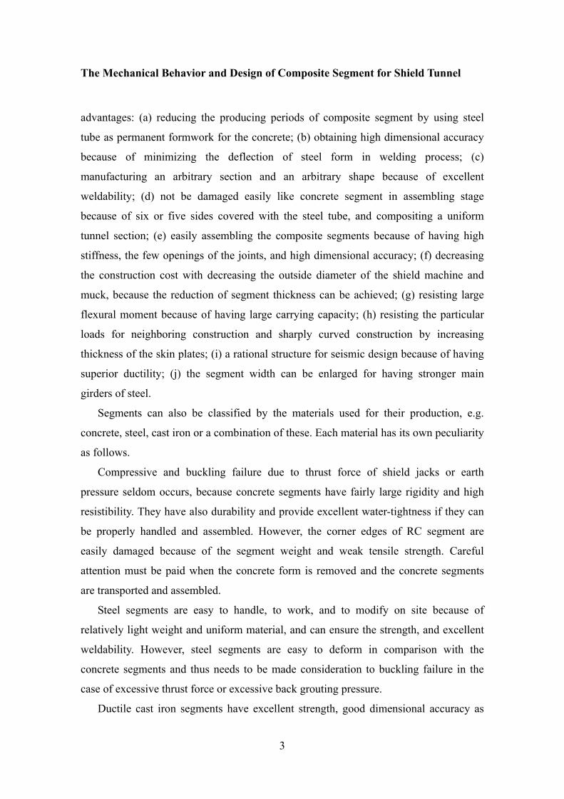
Fig.1.1 Schematic and photo of composite segments.……………….…………………...1
Fig.2.1 Stress-Strain curve of the structural steel..………………....……………….......9
Fig.2.2 Von Mises' yield criterion.………………......………………………………......11
Fig.2.3 Stress-strain curves for unconfined concrete………………..........…………….14
Fig.2.4 CFST member………………......………………........……….………………...18
Fig.2.5 Buyukozturk yield and failure envelopes for concrete…………………............22
Fig.2.6 Shear connectors…………………………….……………….…………………23
Fig.2.7 Load-slip curves for shear studs……………………………….………….........26
Fig.3.1 Manufacturing process of Closed-composite segment…..……………………...35
Fig.3.2 Detail of Closed-composite segment specimens…………….…………………36
Fig.3.3 Biaxial Structure Test Machine and measuring instruments…..….……..........38
Fig.3.4 Test setup for Closed-composite segment specimens………………………......39
Fig.3.5 The arrangement of displacement transducers…………………………………39
Fig.3.6 The strain gauges arrangement of Closed-composite segment specimens……42
Fig.3.7 The method for determining the yield load from load-deformation curves……43
Fig.3.8 Load-deflection curves at midspan………………...…………………………...48
Fig.3.9 Measured strain distribution on the surfaces of steel plates along the midspan
section……………………………………...…………………………...50
Fig.3.10 Measured strain distribution along the height of main girder and mortar
surfaces…………….……………………………………...…………………51
Fig.3.11 Load-relative slip strain on interface between top skin plate and mortar infill..52
Fig.3.12 Load-strain curves on skin plates and the edge of main girders……...….........52
Fig.3.13 Effects of the changing thicknesses of steel tube on ultimate carrying
capacity..……………………………………….....…………………………..53
Fig.3.14 Failure modes of the Closed-composite segment specimens………………..54
Fig.4.1 Finite element model of Closed-composite segment…….…..………………..58
Fig.4.2 Von Mises yield surface in the principal stress space.….……………………….59
Fig.4.3 Concrete failure surface in the principal stress space.….……………………….59
Fig.4.4 Stress-strain relation for unconfined concrete under uniaxial compression.....61
X
Fig.4.5 MSC.Marc ‘Continuous’ friction model through Eq. (4.10)..………………......64
Fig.4.6 Stick-Slip friction procedure in MSC.Marc……..…………………………….66
Fig.4.7 Load-deflection curves for Case15 Closed-segment specimen from different
analyses……….…..……………………….……..…………………………….69
Fig.4.8 Load-deflection curves for tested Closed-segment specimens at midspan…......72
Fig.4.9 Relative slip distribution for Closed-segment specimens without shear studs of
Case10………………….…..……………………….……..……………………74
Fig.4.10 Relative slip distribution for Closed-segment specimens with shear studs of
Case14……………….…..……………………….……..……………………75
Fig.4.11 Load-relative slip relationship for Closed-segment specimens with shear
studs……………….…..……………………….……..……………………75
Fig.4.12 Strain distribution for main girder of Closed-composite segment specimens...76
Fig.4.13 Local buckling of Closed-composite segment specimens without shear studs..77
Fig.4.14 Local buckling of Closed-composite segment specimens with shear studs…...77
Fig.4.15 Concrete infill failure of Closed-composite segment specimens…………….78
Fig.4.16 Contact status of Closed-composite segment specimens……………………...79
Fig.4.17 x-directional stress in skin plates of Closed-composite segment specimens...80
Fig.4.18 Effect of friction on the stiffness of Closed-composite segment specimens…..81
Fig.5.1 Calculation model for the composite segment………………………………….85
Fig.5.2 Kinematic of composite segment…….……………………………………......88
Fig.5.3 Strain distribution of composite segment…………………………………......88
Fig.5.4 Load definitions.………………………………………..…………………........91
Fig.5.5 Calculation model for additional moment………………..…………………......99
Fig.5.6 Discretization of composite section…………………….………..………........100
Fig.5.7 Strain and stress distribution of composite segment……………………........102
Fig.5.8 Bending moment-curvature curves of Closed-composite segments...…….......107
Fig.5.9 Load-deflection curves of Closed-composite segments at midspan.....….........108
Fig.6.1 Manufacturing process of SSPC segment……………………….…………….111
Fig.6.2 Detail of SSPC segment specimen…………………..…………………….......112
Fig.6.3 Test setup for SSPC segment specimens…………..…………………………..113
Fig.6.4 The arrangement of measuring instruments on SSPC segment specimens…....114
XI
Fig.6.5 Load-deflection curves of SSPC segment specimens at midspan.….…………115
Fig.6.6 Measured strain distribution along the height main girder…………..…….....116
Fig.6.7 Failure modes of SSPC segment specimens………………..…………….....117
Fig.6.8 Finite element model of an SSPC segment…………….……………….....118
Fig.6.9 Load-deflection curves for tested SSPC segment specimens at midspan……119
Fig.6.10 Load-relative slip relationship for SSPC segment specimens…..……………119
Fig.6.11 Strain distribution for main girder of SSPC segment specimens………….....120
Fig.6.12 Concrete infill failure of SSPC segment specimens………..…………….....121
Fig.6.13 Contact status of SSPC segment specimens………………………………...122
Fig.6.14 x-directional stress in steel tube of SSPC segment specimens….…….........123
Fig.6.15 DRC segment..……………………………………...……………………….123
Fig.6.16 Arrangement of the discharge channel tunnel and ground condition of 4th
section..……………………………………...……………………………..124
Fig.6.17 Segmental ring arrangement…………………………………………………125
Fig.6.18 Configuration and reinforcing bar layout of A1P~A6P segments…………..126
Fig.6.19 Configuration and reinforcing bar layout of DRC segment specimens...……127
Fig.6.20 Test setup for DRC segment specimens…………..………..........................129
Fig.6.21 Testing steps.………..................................................………..........................130
Fig.6.22 The arrangement of displacement transducers on DRC segment specimens...130
Fig.6.23 The arrangement of strain gauges on DRC segment specimens………..……132
Fig.6.24. Load-deflection curves of DRC segment specimens at midspan………......133
Fig.6.25. Measured strain distribution…………………………...………………….....135
Fig.6.26. Load-relative slip curves of DRC segment specimens……………………..137
Fig.6.27. Failure modes under combined positive bending and axial loads…………138
Fig.6.28 Finite element model of a DRC segment…………………..……….....139
Fig.6.29 Load-deflection curves for tested DRC segment specimens at midspan…..140
Fig.6.30 Load-relative slip relationship for DRC segment specimens………………...141
Fig.6.31 Strain distribution for the members of DRC segment specimens…………...143
Fig.6.32 Concrete infill failure of DRC segment specimens………..……………….144
Fig.6.33 Contact status of DRC segment specimens…………………….……………145
Fig.6.34 x-directional stress in skin plate of DRC segment specimens………………146
XII
Fig.6.35 Bending moment-curvature curves of composite segments….………………150
Fig.6.36 Load-deflection curves of composite segments at midspan……………….…151
Fig.7.1 Flow chart of shield tunnel lining design….………………….………………154
Fig.7.2 Flow chart of calculation of the loads…….………………….………………156
Fig.7.3 Calculation model of loosing earth pressure.………………….………………158
Fig.7.4 Structural models of the segmental lining………………….………………163
Fig.7.5 Concept of the additional rate of bending rigidity…………….………………164
Fig.7.6 Stress condition of joint member..……………….…………….………………167
Fig.7.7 Modeled joint member by springs..……………..…………….………………167
Fig.7.8 Bolt and nut……………………….……………..…………….………………168
Fig.7.9 Stress-strain curve………………...……………..…………….………………181
Fig.7.10 Ground condition………………..……………..…………….………………185
Fig.7.11 Structural model………………..……………..…………….………………187
Fig.7.12 Schematic of joint…...…………..……………..…………….………………187
Fig.7.13 Distributions of member forces of A-Ring in circumferential direction…190
Fig.7.14 Distributions of member forces of B-Ring in circumferential direction…191
Fig.7.15 Contour of member forces of segmental lining assembled in a staggered
pattern…...…………..……………..…………….……………………….…192
Fig.7.16 Transition of ultimate limit states for RC segment…….…………………193
Fig.7.17 Section of RC segment and arrangement of main reinforcements…………194
Fig.7.18 Axial force-moment interaction diagram of RC segment.…………………194
Fig.7.19 Transition of ultimate limit states for Closed-composite segment…………196
Fig.7.20 Resultant axial force in each element………………………….…………197
Fig.7.21 Distribution of connectors in segment with distributed loads…….…………197
Fig.7.22 Section of Closed-composite segment and arrangement of shear studs……199
Fig.7.23 Axial force-moment interaction diagram of Closed-composite segment……199
XIII
List of Tables
Table1.1 Conduits under national roads in the wards of Tokyo………………..………...1
Table2.1. The parameters of unconfined concrete……………………………………....13
Table2.2. Stress-Strain models for confined concrete based on Sargin et al…………....15
Table2.3. Stress-Strain models for confined concrete based on Kent and Park………...16
Table2.4. Stress-Strain models for confined concrete based on Kent and Park………...17
Table2.5 Experimental and analytical curve parameters of Candappa et al…………20
Table2.6 Experimental and analytical curve parameters of Attard-Setunge……………20
Table2.7 Experimental and analytical curve parameters of Imran-Pantazopoulou……..20
Table2.8 Coefficients for static stiffness of a shear stud per Equation 2.20..……...26
Table3.1 Details of Closed-segment specimens…………………….…………………36
Table3.2 Mechanical material properties for Closed-composite segment specimens....37
Table3.3 Experimental results of Closed-composite segment specimens.…………......44
Table5.6 Comparison of elastic bending capacities of composite segment specimens..105
Table5.7 Comparison of ultimate bending capacities of composite segment specimens
...…………………………...…………………………106
Table6.1 Details of SSPC segment specimens.……………...………………………...112
Table6.2 Mechanical material properties for SSPC segment specimens………….....112
Table6.3 Experimental results of SSPC segment specimens...………….....…….……115
Table6.4 Details of DRC segment specimens……….……….………………………128
Table6.5 Mechanical material properties for DRC segment specimens.………….......128
Table6.6 Comparison of elastic bending capacities of composite segment specimens..148
Table6.7 Comparison of ultimate bending capacities of composite segment specimens
...…………………………...…………………………149
Table7.1 Earth pressure acting on the lining by Terzaghi…………………………..157
Table7.2. Coefficient (λ ) of lateral earth pressure and coefficient ( k ) of ground reaction
...…………………………...…………………………157
Table7.3. Examples of notation used in the guidelines (Soil condition)...…………….160
Table7.4. Examples of notation used in the guidelines………….……………….......161
XIV
Table7.5 Equations of member forces for conventional model/modified conventional
model...……...…….....…………………………...…………………………165 Table7.6 Effective ratio of the bending rigidity of η and additional rate of ζ ….……166 Table7.7 Spring constant of soil reaction...……………………………………………170
Table7.8 Allowable stresses of concrete for segment (N/mm2)…………………….....171
Table7.9 Allowable stresses of cast-in-place reinforced concrete (N/mm2)….…….....172
Table7.10 Allowable stresses of cast-in-place plain concrete (N/mm2)…..….…….....172
Table7.11 Allowable stresses of reinforcement(N/mm2)..……….…………………….172
Table7.12 Allowable stresses of steel material and welds(N/mm2).…………………173
Table7.13 Allowable buckling stresses(N/mm2)………………...………………….....173
Table7.14 Allowable stresses for local buckling of steel segment(N/mm2)……….....174
Table7.15 Allowable stresses of spheroidal graphite cast iron (N/mm2)..……….....174
Table7.16 Allowable stresses for buckling of spheroidal graphite cast iron (N/mm2)...174
Table7.17 Allowable stresses for buckling of ductile cast iron segment (N/mm2)….....175
Table7.18 Allowable stresses of steel casting for welded structure (N/mm2)…..….....175
Table7.19 Allowable stresses of bolt (N/mm2)...…..............................................….....175
Table7.20 Characteristic values of the strength of concrete for segment (N/mm2)...176
Table7.21 Characteristic values of the strength of cast-in-place reinforced concrete
(N/mm2) ...…..............................................…..... .........................…...........177
Table7.22 Characteristic values of the strength of reinforcement (N/mm2)…………...177
Table7.23 Characteristic values of the strength of steel material and welds (N/mm2)...178
Table7.24 Characteristic values of steel buckling(N/mm2)…………..........................178
Table7.25 Characteristic values for local buckling of steel segment(N/mm2)..........179
Table7.26 Characteristic values of the strength of spheroidal graphite cast iron
(N/mm2)....…..............................................…...............................…...........179
Table7.27 Characteristic values of the strength for buckling (N/mm2)………..........179
Table7.28 Characteristic values for local buckling of ductile cast iron segment (N/mm2)
....…..............................................…...............................…...........180
Table7.29 Characteristic values of steel casting for welded structure(N/mm2)....180
Table7.30 Characteristic values of the strength of bolt(N/mm2)………………..180
Table7.31 Elastic modulus of concrete (segment) (N/mm2)……………………181
XV
Table7.32 Elastic modulus of steel, reinforcement, and spheroidal graphite cast iron
(N/mm2) ....…..............................................…...............................…..........181
Table7.33 Poisson’s ratio………………………………………………………………181
Table7.34 Nominal standard for material factor………………………………………182
Table7.35 Nominal standard for member factor (Concrete segment)…………………182
Table7.36 Nominal standard for member factor (Steel and cast iron segment)………183 Table7.37 Nominal standard for load factor fγ ……………………..…………………183
Table7.38 Nominal standard for structural analysis factor….…………………………183
Table7.39 Nominal standard of structure factor...…………………..…………………184
Table7.40 Combined load case……………….....…………………..…………………185
Table7.41 Spring constant of soil reaction……..…………………..…………………187
Table7.42 Member forces of segmental lining (A-Ring)…….……..…………………188
Table7.43 Comparison of structural type…………………….……..…………………200


XVII
NOTATION
The following notation is used in this book. Generally, only one meaning is assigned
to each symbol, but in cases where more than one meaning is possible, then the correct
one will be evident from the context in which it is used.
A =Area; constant of material
bA =Area of bottom skin plate section
cA =Area of concrete section
cuA =Area of uncracked concrete section
mbA =Area of main girder section in tension
mtA =Area of main girder section in compression
tA =Area of top skin plate section
shA =Cross-sectional area of the shank of a shear stud
B =Width of segment; constant of material; width or span of opening
C =Constant of material; ratio
D =Diameter of an equivalent circular section
D0 =Diameter of segmental lining
hdd =Diameter of the head of a shear stud
shd =Diameter of the shank of a shear stud
cE =Elastic modulus of the concrete
iE =Initial tangent modulus
fE =Secant modulus of concrete measured at peak stress
sE =Elastic modulus of the steel
stE =Strain hardening modulus of steel
EA =Axial rigidity
EI =Bending rigidity
cf = Compressive strength of unconfined concrete
ccf = Compressive strength of confined concrete
tf ′ =Tensile strength of unconfined concrete
XVIII
lxf , lyf =Lateral confining pressures in the two orthogonal directions
ypf =Yield stress of steel plate
udf ′ =Post-buckling stress of steel plate
H =Height of channel connector
Ht =Height of opening
shh =Height of the shank of a shear stud
bI =Moment of inertia of the bottom skin plate section
cuI =Moment of inertia of the uncracked concrete section
mbI =Moment of inertia of main girder section in tension
mtI =Moment of inertia of main girder section in compression
tI =Moment of inertia of the top skin plate section
0K =Ratio between lateral earth pressure and vertical earth pressure
k = Coefficient of ground reaction; local buckling coefficient;
bk =Axial rigidity of bolt cak =Rigidity of axial spring csk =Rigidity of shear spring ckθ =Rigidity of rotational spring
dk =Shape factor
puk =Axial rigidity of joint plate in compression
plk =Axial rigidity of joint plate considering the initial tightening bolt induced compressive strain released
siK =Initial stiffness of a shear stud
L =Length of segment
rL =Length of channel shear connector
bM =Moment carried by the bottom skin plate
cM =Moment carried by the concrete infill
tM =Moment carried by the top skin plate
mbM =Moment carried by the main girders in tension
mtM =Moment carried by the main girders in compression
N-A =Position of neutral axis
n =Number of shear connectors in a group; modular ratio;
XIX
P =Applied load
P0 =Surcharge
uP =Ultimate tensile strength of a shear stud
uQ =Ultimate shear strength of a shear stud
nQ =Ultimate shear strength of a channel shear connector
q =Shear flow; shear flow force; longitudinal shear force per unit length
0R =Outer radius of the lining
cR =Radius of controid of the lining
r =Radius of the internal corner
ar =Radius of a bolt hole
wr =Radius of a washer
S =Shear force of segmental lining
ults =Slip at fracture
bT =Axial force carried by the bottom skin plate
cT =Axial force carried by the concrete infill
tT =Axial force carried by the top skin plate
mbT =Axial force carried by the main girders in tension
mtT =Axial force carried by the main girders in compression
t =Thickness of plate
tj =Thickness of joint plate
tm =Thickness of main girder
ts =Thickness of skin plate
wt =Thickness of a washer
V = ransverse shear load;
bV =Shear force carried by the bottom skin plate
cV =Shear force carried by the concrete infill
tV =Shear force carried by the top skin plate
mbV =Shear force carried by the main girders in tension
mtV =Shear force carried by the main girders in compression
W =Weight of lining per meter in longitudinal direction

XX
α =A function of uniaxial compressive strength of concrete cf ′
β =Coefficient of variability
Vβ =Reduction factor
tγ =The top relative slip between the top skin plate and concrete infill
bγ =The bottom relative slip between the bottom skin plate and concrete
infill
δ =Deflection ε =Strain
cε =Strain in concrete
,h rupε =Ultimate transverse strain in the steel jacket at rupture σ =Stress
1σ , 2σ , 3σ =Principal stresses
1 2σ ′ ′ =Shear stress
1I =First invariant of stress tensor
2J =Second invariant of stress tensor
φ =Curvature

The Mechanical Behavior and Design of Composite Segment for Shield Tunnel
1
Chapter 1. Introduction 1.1 PREFACE
The subsurface under roads in big cities is already crowded with underground
facilities such as railroads, and tunnels for electricity, gas, communications, sewage and
drainage, and conduits. For example, the subsurface of a national highway in Tokyo has
about 33 km of conduits per kilometer of road as shown in Table1.1. For this reason,
newly constructed infrastructure such as subways etc. must be constructed deeper year
by year in order to avoid those conduits [1].
Table 1.1 Conduits under National Roads in the Wards of Tokyo (161.2km of national road
under direct administration of National Government)
Total length (km) No. of kilometers (km) of underground facilities per one road km
Telephone lines 2684.1 16.7
Electric lines 1660.7 10.3
Gas 325.9 2.0
Water supply lines 364.6 2.3
Sewage lines 315.7 2.0
Total 5351.0 33.3
From MLIT
Note: 1. Statistical data of April, 2004
2. Total length refers to total length of under-road conduits
3. Not include conduits to each building.
The shield tunneling method has rapidly become popular in Japan as an effective
tunneling method in urban and for constructing infrastructures. Recently, it has often
become necessary to construct tunnels under severe conditions and to develop new
techniques because there are some restrictions on the alignment of tunnels and the width
of street where the tunnels are located.
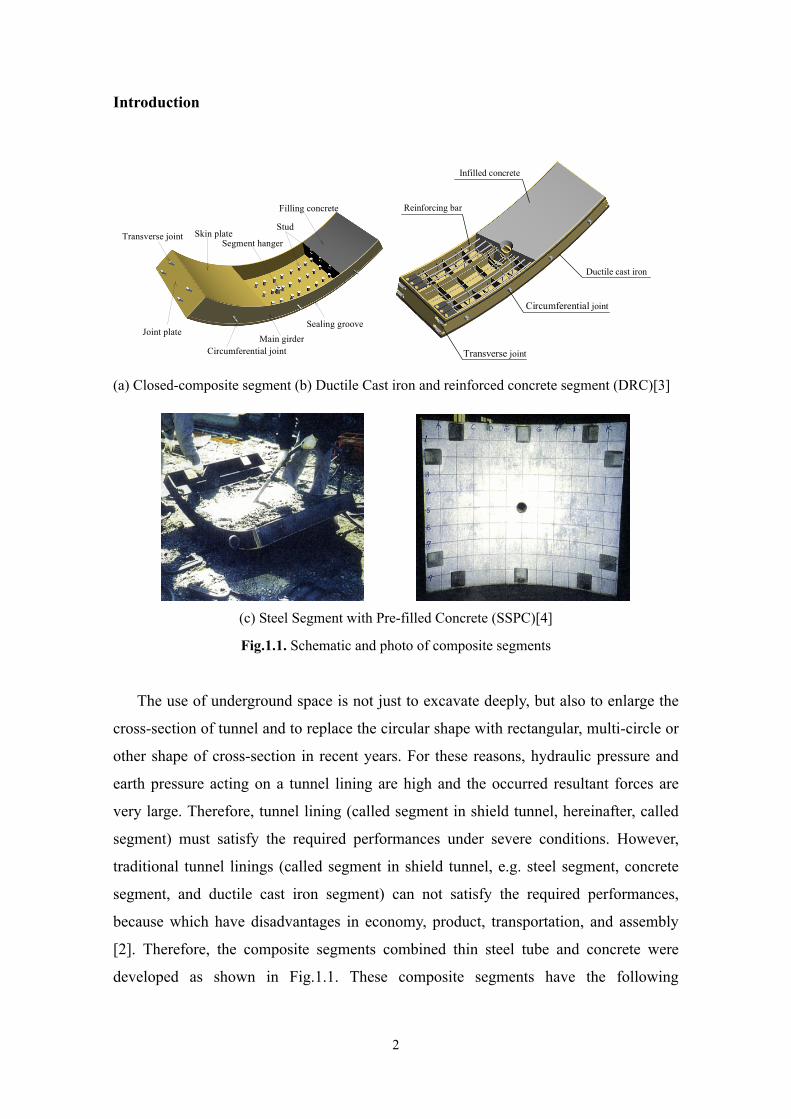
Introduction
2
Transverse joint Skin plate
Main girderCircumferential joint
Sealing grooveJoint plate
Segment hanger
Stud
Filling concrete
Transverse joint
Circumferential joint
Ductile cast iron
Infilled concrete
Reinforcing bar
(a) Closed-composite segment (b) Ductile Cast iron and reinforced concrete segment (DRC)[3]
(c) Steel Segment with Pre-filled Concrete (SSPC)[4]
Fig.1.1. Schematic and photo of composite segments
The use of underground space is not just to excavate deeply, but also to enlarge the
cross-section of tunnel and to replace the circular shape with rectangular, multi-circle or
other shape of cross-section in recent years. For these reasons, hydraulic pressure and
earth pressure acting on a tunnel lining are high and the occurred resultant forces are
very large. Therefore, tunnel lining (called segment in shield tunnel, hereinafter, called
segment) must satisfy the required performances under severe conditions. However,
traditional tunnel linings (called segment in shield tunnel, e.g. steel segment, concrete
segment, and ductile cast iron segment) can not satisfy the required performances,
because which have disadvantages in economy, product, transportation, and assembly
[2]. Therefore, the composite segments combined thin steel tube and concrete were
developed as shown in Fig.1.1. These composite segments have the following
The Mechanical Behavior and Design of Composite Segment for Shield Tunnel
3
advantages: (a) reducing the producing periods of composite segment by using steel
tube as permanent formwork for the concrete; (b) obtaining high dimensional accuracy
because of minimizing the deflection of steel form in welding process; (c)
manufacturing an arbitrary section and an arbitrary shape because of excellent
weldability; (d) not be damaged easily like concrete segment in assembling stage
because of six or five sides covered with the steel tube, and compositing a uniform
tunnel section; (e) easily assembling the composite segments because of having high
stiffness, the few openings of the joints, and high dimensional accuracy; (f) decreasing
the construction cost with decreasing the outside diameter of the shield machine and
muck, because the reduction of segment thickness can be achieved; (g) resisting large
flexural moment because of having large carrying capacity; (h) resisting the particular
loads for neighboring construction and sharply curved construction by increasing
thickness of the skin plates; (i) a rational structure for seismic design because of having
superior ductility; (j) the segment width can be enlarged for having stronger main
girders of steel.
Segments can also be classified by the materials used for their production, e.g.
concrete, steel, cast iron or a combination of these. Each material has its own peculiarity
as follows.
Compressive and buckling failure due to thrust force of shield jacks or earth
pressure seldom occurs, because concrete segments have fairly large rigidity and high
resistibility. They have also durability and provide excellent water-tightness if they can
be properly handled and assembled. However, the corner edges of RC segment are
easily damaged because of the segment weight and weak tensile strength. Careful
attention must be paid when the concrete form is removed and the concrete segments
are transported and assembled.
Steel segments are easy to handle, to work, and to modify on site because of
relatively light weight and uniform material, and can ensure the strength, and excellent
weldability. However, steel segments are easy to deform in comparison with the
concrete segments and thus needs to be made consideration to buckling failure in the
case of excessive thrust force or excessive back grouting pressure.
Ductile cast iron segments have excellent strength, good dimensional accuracy as
Introduction
4
products, and also provide excellent waterproof performance. They, like steel segment,
needs to be made consideration to buckling failure or to apply proper corrosion
protection, when the secondary lining is not executed.
Composite segments are composed of steel tube and concrete or Ductile cast iron
tube and concrete. Although composite segments are more expensive than RC segments,
which take advantage of the speed of construction, light weight and high strength of
steel, and the high-mass, rigidity, damping properties, and economy of concrete. In
addition, composite segments can resist the large sectional force induced by
asymmetrical pressure, high hydraulic pressure and earth pressure, and decrease the
height of the used segment and muck of the excavated tunnel cross-section.
1.2 PURPOSE AND SCOPE OF THIS STUDY
The knowledge of this composite interactions as well as elemental behavior
involved in composite structure has developed rapidly during the past several decades.
Much effort has been put forth to better understand and model the behavior of the
composite structure. Research on the subject has been conducted worldwide (U.S.,
Japan, Canada, Europe and Australia).
However, a rational design method for the composite segments can not be
established, because the mechanical behavior of the composite segments is still not clear.
Especially, it is true problem that how to evaluate the effects of the interface slip and the
confinement effect of steel tube on the deflection of the concrete infill, to install the
number and arrangement of shear connectors, and to evaluate the contributions of
resultant forces in steel tube and concrete infill, and the deflection behavior of
composite section.
In general, many underground structures are designed by the allowable stress design
method. In this method various indeterminate factors such as variations in material
properties, acting loads, precision of estimated design loads, analysis model and
structural calculation method etc., are simply assumed based on factors of safety.
Shield tunnel linings (hereinafter called as segmental rings) consist of segments and
many connecting joints, and show complicated mechanical behavior under combined
The Mechanical Behavior and Design of Composite Segment for Shield Tunnel
5
loads. Meanwhile, it is difficult to precisely define the loads acting on segment rings
due to variation in construction conditions. Therefore, the allowable stress design
method as a simplified solution is still used in the design of segments for shield tunnel.
However, it is possible to predict the variations in acting loads and material
properties etc., because of the high technical developments of FEA and measuring
method for the last few years. Therefore, the allowable stress design method is not
rational in economy, because it is not able to directly assess the variations in material
strength, member size, and loads etc. On the contrary, the limit state design is able to
assess the variations in material strength, member size, and loads etc using factors of
safety based on the theories of probability, statistics, and reliability.
The limit state design requires the structure to satisfy two principal criteria: the
ultimate limit state (ULS) and the serviceability limit state (SLS). A limit state is a set of
performance criteria (e.g. vibration levels, deflection, strength, stability, buckling,
twisting, and collapse) that must be met when the structure is subject to loads.
To satisfy the ultimate limit state, the structure must not collapse when subjected to
the peak design load for which it was designed. A structure is deemed to satisfy the
ultimate limit state criteria if all factored bending, shear, and tensile or compressive
stresses are below the factored resistance calculated for the section under consideration.
The limit state criteria can also be set in terms of stress rather than load. Thus the
structural element being analyzed (e.g. a beam or a column or other load bearing
element, such as walls) is shown to be safe when the factored loads are less than their
factored resistance.
To satisfy the serviceability limit state criteria, a structure must remain functional
for its intended use subject to service loads, and as such the structure must not cause
occupant discomfort under design life.
It is true problem that the limit state design is not currently used in the segment
design for shield tunnel. Therefore, one of the purposes of developing a mechanical
model for composite segment is to provide tools suitable for limit state design. The
paper does not address safety coefficients as its purpose is to underscore the phenomena
involved in the issue rather than measuring structural safety.
The purpose of this study can be summarized as follows:
Introduction
6
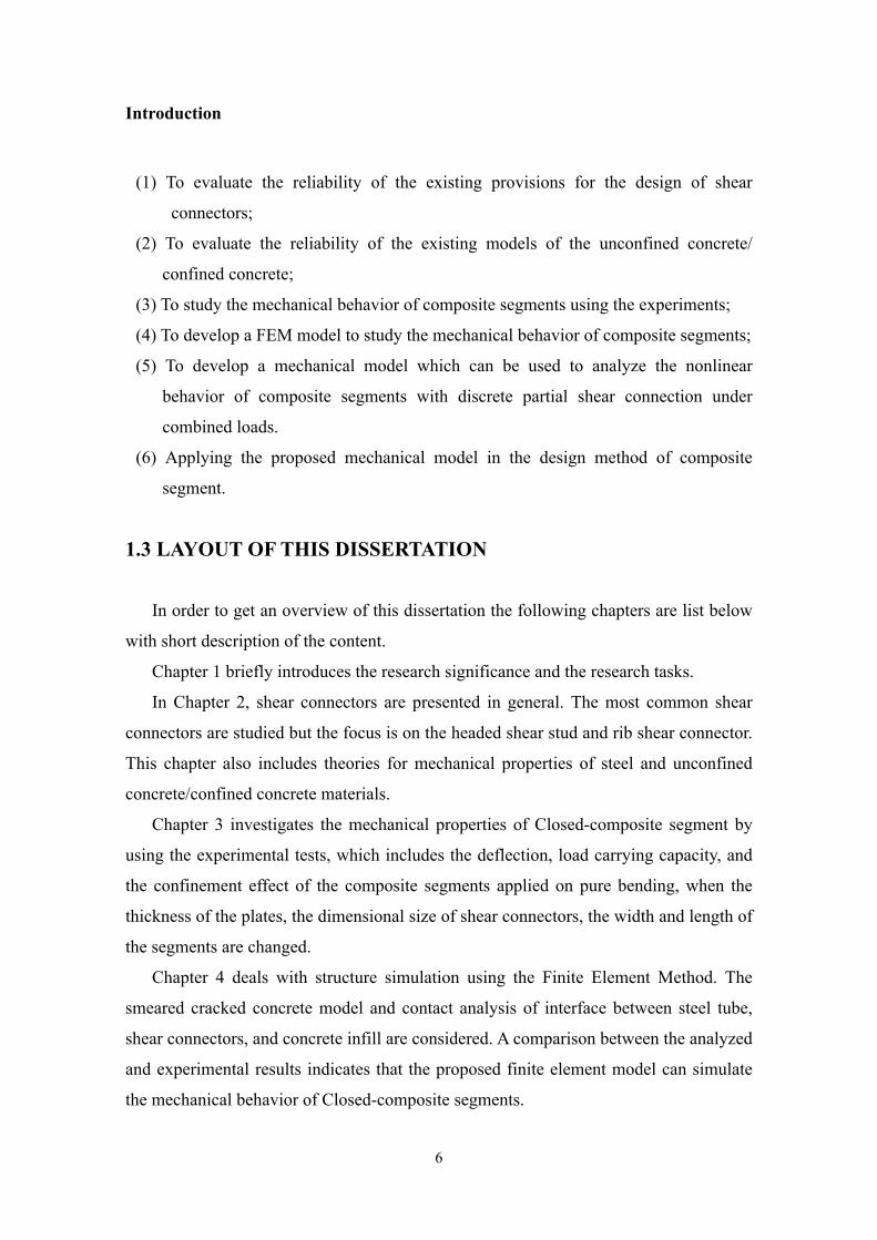
(1) To evaluate the reliability of the existing provisions for the design of shear
connectors;
(2) To evaluate the reliability of the existing models of the unconfined concrete/
confined concrete;
(3) To study the mechanical behavior of composite segments using the experiments;
(4) To develop a FEM model to study the mechanical behavior of composite segments;
(5) To develop a mechanical model which can be used to analyze the nonlinear
behavior of composite segments with discrete partial shear connection under
combined loads.
(6) Applying the proposed mechanical model in the design method of composite
segment.
1.3 LAYOUT OF THIS DISSERTATION
In order to get an overview of this dissertation the following chapters are list below
with short description of the content.
Chapter 1 briefly introduces the research significance and the research tasks.
In Chapter 2, shear connectors are presented in general. The most common shear
connectors are studied but the focus is on the headed shear stud and rib shear connector.
This chapter also includes theories for mechanical properties of steel and unconfined
concrete/confined concrete materials.
Chapter 3 investigates the mechanical properties of Closed-composite segment by
using the experimental tests, which includes the deflection, load carrying capacity, and
the confinement effect of the composite segments applied on pure bending, when the
thickness of the plates, the dimensional size of shear connectors, the width and length of
the segments are changed.
Chapter 4 deals with structure simulation using the Finite Element Method. The
smeared cracked concrete model and contact analysis of interface between steel tube,
shear connectors, and concrete infill are considered. A comparison between the analyzed
and experimental results indicates that the proposed finite element model can simulate
the mechanical behavior of Closed-composite segments.

The Mechanical Behavior and Design of Composite Segment for Shield Tunnel
7
In Chapter 5, a nonlinear fiber element analysis method is developed for the
inelastic analysis and design of concrete infill steel tubular composite segments with
local buckling and slips effects. Sectional geometry, residual stresses and strain
hardening of steel tubes and confined concrete models were considered in the proposed
mechanical model. The local buckling, slip and effective strength formulas are
incorporated into the nonlinear analysis procedures to account for local buckling and
slip effects on the strength and ductility performance of composite segments under
combined loads. Comparisons are made between the experimental results of
Closed-composite segment and the mechanical predictions of behavior using the
proposed method. Good agreement is found and this indicates that the proposed method
is suitable for general analysis of Closed-composite segment.
Chapter 6 deals with structure simulation of SSPC segment and DRC segment using
FEM and the proposed method. Good agreement is found and this indicates that the
proposed finite element model and the proposed mechanical model is suitable for
general analysis of others type composite segments.
Chapter 7 deals with the cross-section design of composite segment of the fourth
section of the Tokyo Metropolitan Area Outer Underground Discharge Channel based
on the above proposed model.
Finally, Chapter 8 summarizes the outcomes of this research work, draws associated
conclusions.
1.4 REFERENCES 1) Ministry of Land, Infrastructure and Transport Government of Japan (MLIT), 2005.
Progress in the use of the Deep Underground.
2) Japan Society of Civil Engineers, 2006. Standard specifications for tunneling-2006,
Shield tunnels.
3) Masami, Shirato, et al.2003. Development of new composite segment and application
to the tunneling project. Journal of JSCE, No.728, 157-174. (In Japanese)
4) Japan Steel Segment Association (JSSA), 1995. The report of development of Steel
Segment with Pre-filled Concrete(SSPC) . (In Japanese)

The Mechanical Behavior and design of Composite Segment for Shield Tunnel
9
Chapter 2. Material Properties
2.1 STEEL COMPONENT
The primary purpose of the steel element in a composite beam is to carry tensile
stresses, while in composite columns the steel shares in the carrying of compressive
stresses with the concrete. It is the high strength of the steel, coupled with its ductility,
which makes it such a vital component of a composite member.
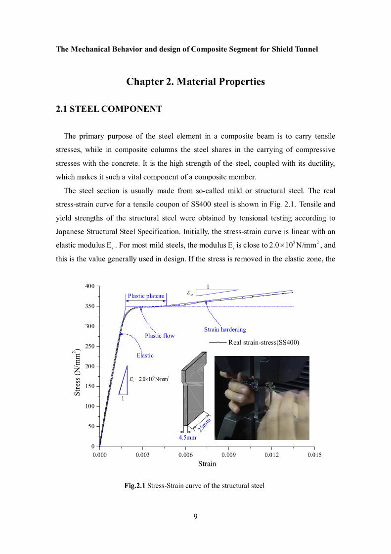
The steel section is usually made from so-called mild or structural steel. The real
stress-strain curve for a tensile coupon of SS400 steel is shown in Fig. 2.1. Tensile and
yield strengths of the structural steel were obtained by tensional testing according to
Japanese Structural Steel Specification. Initially, the stress-strain curve is linear with an
elastic modulus sE . For most mild steels, the modulus sE is close to 5 22.0 10 N/mm× , and
this is the value generally used in design. If the stress is removed in the elastic zone, the
0.000 0.003 0.006 0.009 0.012 0.0150
50
100
150
200
250
300
350
400
4.5mm
25mm
Strain hardeningPlastic flow
Plastic plateau
Elastic
stE1
1
5 22.0 10 N/mmsE = ×
Stre
ss (N
/mm
2 )
Strain
Real strain-stress(SS400)
Fig.2.1 Stress-Strain curve of the structural steel
Material Properties
10
steel recovers perfectly on unloading. The linear elastic behavior continues until the yield stress yf is reached, at a yield strain y sf / Eyε = . Further straining results in plastic
flow with little or no increase in stress until the strain hardening strain is reached. The
stress in the steel then increases until its ultimate tensile strength is attained. The
cross-section then begins to neck down, with large reductions in the cross-sectional area,
until the steel finally fractures.
Undoubtably, the most important strength property of the steel element is its yield strength yf . In most composite applications, this value is usually between about 250 and
350 N/mm2, although in some structures it may be higher, and it depends largely on the
chemical constituents of the steel, primarily carbon and manganese. The yield stress is
increased with increased amounts of these elements, as well as the amount of working
which takes place during the rolling process. Higher yield stresses are also observed
under higher strain rates /d dtε of loading. Generally speaking, the higher the yield
stress, the less is the plastic plateau in Fig. 2.1 and consequently the ductility is
decreased. Because of this, many structural steel standards place limits on the yield
stress of the steel that may be used, since ductility is a desired requirement in structural
design.
Under uniaxial compression, the stress-strain characteristics of the steel section are
roughly the same as those in tension up to the plastic range. The yield stress yf determined from a tensile strength test is generally accepted as being the same
for compression, along with the elastic modulus sE . However, the steel section under
compression is often subjected to buckling or instability effects.
Quite often, it is appropriate to treat the stress in the steel section as being uniaxial.
However, the general state of stress at a point in a thin-wall member is one of biaxial
tension and/or compression, and yielding under these conditions is not so simply
determined, which uses the notation of Trahair and Bradford [1,2]. The most accepted
theory of two-dimensional yielding under biaxial stresses is the von Mises' maximum
distortion energy theory, and the stresses at yield according to this theory satisfy the
condition
2 2 2 21 1 2 2 1 23 yfσ σ σ σ σ′ ′ ′ ′ ′ ′− + + = (2.1)
The Mechanical Behavior and design of Composite Segment for Shield Tunnel
11
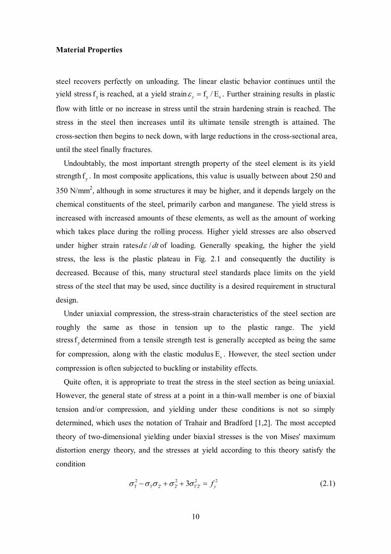
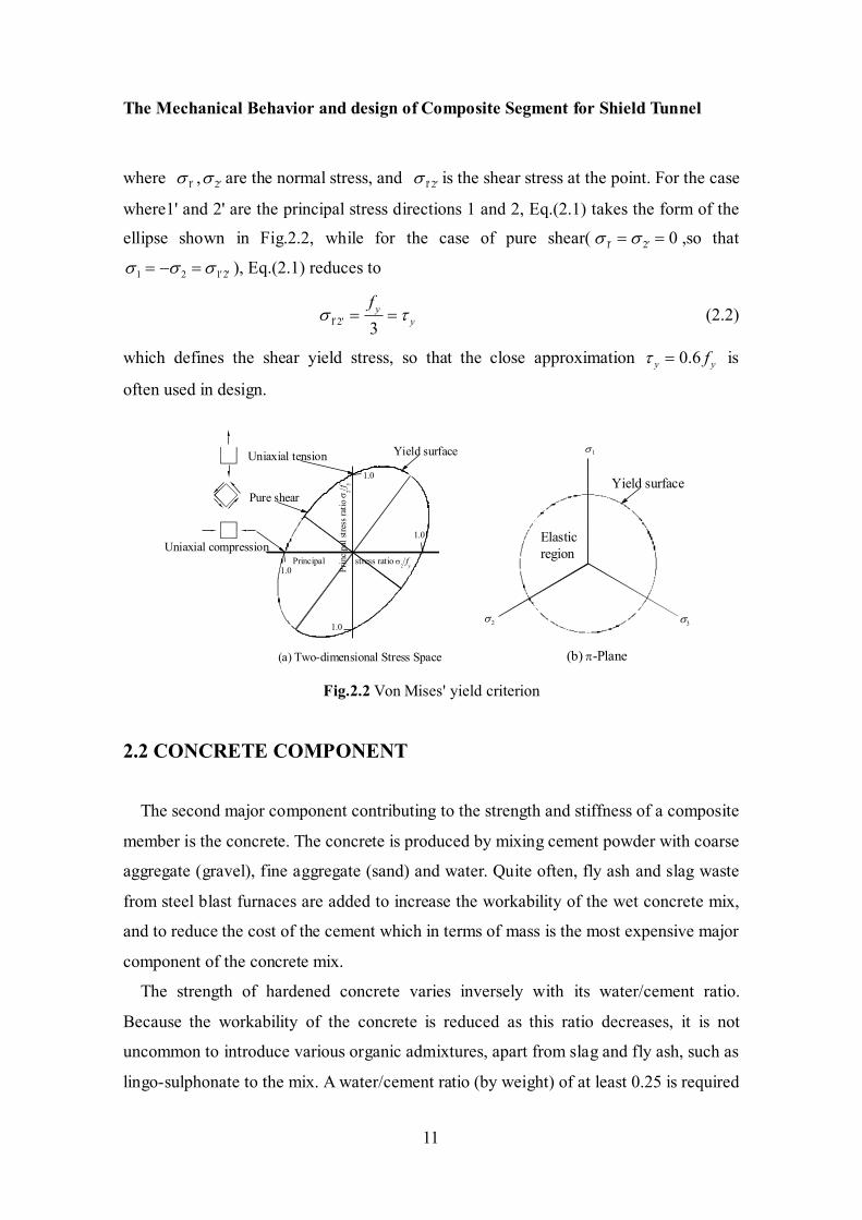
where 1σ ′ , 2σ ′ are the normal stress, and 1 2σ ′ ′ is the shear stress at the point. For the case
where1' and 2' are the principal stress directions 1 and 2, Eq.(2.1) takes the form of the
ellipse shown in Fig.2.2, while for the case of pure shear( 1 2 0σ σ′ ′= = ,so that
1 2 1 2σ σ σ ′ ′= − = ), Eq.(2.1) reduces to
1 2 3y
y
fσ τ′ ′ = = (2.2)
which defines the shear yield stress, so that the close approximation 0.6y yfτ = is
often used in design.
(a) Two-dimensional Stress Space
Yield surface
Prin
cipa
l stre
ss ra
tio σ
2/f y
Principal stress ratio σ2/f
y1.0
1.0
1.0
1.0
Uniaxial compression
Pure shear
Uniaxial tension
1σ
2σ 3σ
Yield surface
Elastic region
(b) π-Plane
Fig.2.2 Von Mises' yield criterion
2.2 CONCRETE COMPONENT
The second major component contributing to the strength and stiffness of a composite
member is the concrete. The concrete is produced by mixing cement powder with coarse
aggregate (gravel), fine aggregate (sand) and water. Quite often, fly ash and slag waste
from steel blast furnaces are added to increase the workability of the wet concrete mix,
and to reduce the cost of the cement which in terms of mass is the most expensive major
component of the concrete mix.
The strength of hardened concrete varies inversely with its water/cement ratio.
Because the workability of the concrete is reduced as this ratio decreases, it is not
uncommon to introduce various organic admixtures, apart from slag and fly ash, such as
lingo-sulphonate to the mix. A water/cement ratio (by weight) of at least 0.25 is required
Material Properties
12
to hydrate the cement properly, and water/cement ratios in the range 0.35 to 0.50 are
commonly used for normal strength concretes.
Limit states or load and resistance factor design necessitate that both strength and
stiffness requirements of the concrete are met. In achieving these requirements, it must
be noted that the properties of the concrete.
2.2.1 Concrete properties
Concrete is a variable material, and identical strength tests undertaken at a given time
after casting show significant variability. However, the mean strength cmf in uniaxial
compression increases with concrete age. The major shortfall of the concrete portion of
a composite member is its low tensile strength, so that strengths usually quoted for
concrete are in terms of the uniaxial compressive strength.
Concrete compressive strengths are determined by testing specimens of identical
shape, which have been cured under the same conditions, in a stiff hydraulic testing
machine. In Japan, the standard test specimen is a 50/100 mm diameter cylinder, which
is 100/150 mm high. North America and in Australia, the standard test specimen is a
150 mm diameter cylinder, which is 300 mm high with its top capped with sulphur. On
the other hand, British practice is to use a 150 mm sided cube. Because of the shape
effects, the cube strengths cuf are higher than the cylinder strengths cf . Generally
throughout this paper, reference will be made to cylinder strengths of Japanese standard
test specimen.
It is well known that confinement of concrete is effective in increasing its strength
and deformation capacity. It is generally agreed that the strength and stiffness of
confined concrete increases with the stiffness of the confining material as well as the
compressive strength of the unconfined concrete. Because of confinement effect, both
the unconfined and confined properties of concrete must be addressed. These properties
are studied in the following.
(a) Constitutive Models for Unconfined Concrete
In the concrete compressive stage, the stress-strain relation proposed by Carreira and
Chu [3] has been employed to model the elastic-plastic material characteristics with

The Mechanical Behavior and design of Composite Segment for Shield Tunnel
13
strain softening:
1
cc
cc
c
c
f
α
εαε
σεαε
⎛ ⎞′ ⎜ ⎟⎜ ⎟′⎝ ⎠=
⎛ ⎞− + ⎜ ⎟⎜ ⎟′⎝ ⎠
(2.3)
where cσ is compressive stress in concrete( 2N/mm ); cε is strain in concrete; cf ′ is
uniaxial compressive strength of concrete( 2N/mm ); cε ′ is strain corresponding to cf ′ ;
and α as a function of uniaxial compressive strength of concrete cf ′ , can be estimated
by the following formula[4] 3
1.55cfαβ′⎡ ⎤
= +⎢ ⎥⎣ ⎦
(2.4)
The coefficient of variability β increases when increasing the compressive strength of
the concrete. Therefore, if 221.0N/mmcf ′ = , 22.0β = and if 280.0N/mmcf ′ = , 71.4β = ,
for intermediate stress gradients, β can be determined by linear interpolations. The
proposed relation for β was found using regression analysis based experimental values
shown in Table 2.1.
Table 2.1. The parameters of unconfined concrete
Compressive strength
2(N/mm )cf ′
Elastic Modulus
2(kN/mm )cE
Tensile strength 2(N/mm )tf ′
Peak strain
cε ′ Unit weight
(kN/m3) β
21 22 1.75 0.00205 23 22.0
24 25 1.91 0.00219 23 24.5
27 26 2.07 0.00232 23 27.1
30 28 2.22 0.00245 23 29.6
40 31 2.69 0.00283 23 37.3
50 33 3.12 0.00316 23 39.5
60 35 3.53 0.00346 23 46.5
70 37 3.91 0.00374 23 55.0
80 39 4.27 0.00400 23 71.4
6447.2 10c cfε −′ ′= × or ci2 /cf E′ [5]; ciE is the initial tangent modulus of concrete
Material Properties
14
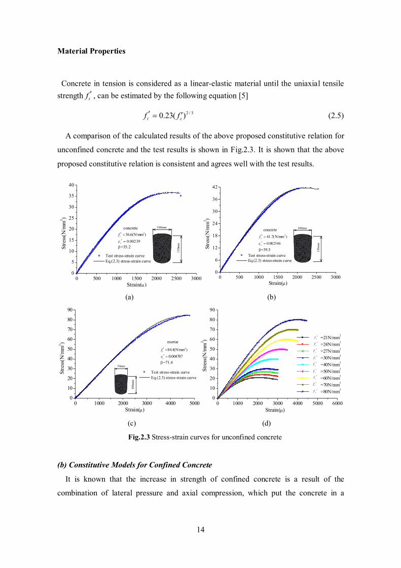
Concrete in tension is considered as a linear-elastic material until the uniaxial tensile strength tf ′ , can be estimated by the following equation [5]
2 / 30.23( )t cf f′ ′= (2.5)
A comparison of the calculated results of the above proposed constitutive relation for
unconfined concrete and the test results is shown in Fig.2.3. It is shown that the above
proposed constitutive relation is consistent and agrees well with the test results.
0 500 1000 1500 2000 2500 30000
5
10
15
20
25
30
35
40
236.6(N/mm )cf ′ =0.00239cε ′ =
concrete
β=35.2
150m
m
100mm
Stre
ss(N
/mm
2 )
Strain(μ)
Test stress-strain curve Eq.(2.3) stress-strain curve
0 500 1000 1500 2000 2500 30000
6
12
18
24
30
36
42
0.002346cε ′ =
241.7(N/mm )cf ′ =
concrete
β=39.5 150m
m
100mm
Stre
ss(N
/mm
2 )
Strain(μ)
Test stress-strain curve Eq.(2.3) stress-strain curve
(a) (b)
0 1000 2000 3000 4000 50000
10
20
30
40
50
60
70
80
90
0.004707cε ′ =
284.4(N/mm )cf ′ =
mortar
β=71.4
100m
m
50mm
Stre
ss(N
/mm
2 )
Strain(μ)
Test stress-strain curve Eq.(2.3) stress-strain curve
0 1000 2000 3000 4000 5000 60000
10
20
30
40
50
60
70
80
90
cf ′
cf ′
cf ′cf ′
cf ′
cf ′
cf ′
cf ′cf ′
Stre
ss(N
/mm
2 )
Strain(μ)
=21N/mm2
=24N/mm2
=27N/mm2
=30N/mm2 =40N/mm2
=50N/mm2
=60N/mm2
=70N/mm2
=80N/mm2
(c) (d) Fig.2.3 Stress-strain curves for unconfined concrete
(b) Constitutive Models for Confined Concrete
It is known that the increase in strength of confined concrete is a result of the
combination of lateral pressure and axial compression, which put the concrete in a

The Mechanical Behavior and design of Composite Segment for Shield Tunnel
15
triaxial stress state. The lateral pressure is provided by lateral steel reinforcement and a
steel jacket. Based on the test results, various stress-strain models for confined concrete
have been proposed, such as Sheikh and Uzumeri[6], Mander et al.[7], and Cusson and
Paultre[8]models. Existing stress-strain models for confined, unconfined normal, as
well as high strength concrete can be divided into three broad categories. One group of
researchers used a form of equation proposed by Sargin et al.[9](Table 2.2). The second
group of researchers proposed second order parabola for the ascending branch and a
straight line for the descending branch and their studies were based on equations
proposed by Kent and Park [10]( Table2.3). The third group developed stress-strain
relations based on equations suggested by Popovics[11] (Table 2.4).
In these stress-strain models, 1 1( , )σ ε are the coordinates of any point in the
stress-strain curve, coε is the peak axial strain of unconfined concrete strength cf , ccε
is the peak axial strain of confined concrete strength ccf , lf is the confining pressure,
cE is the elastic modulus of concrete, iE is the initial tangent modulus, and fE is the
secant modulus of concrete measured at peak stress.
Table 2.2. Stress-Strain Models for Confined Concrete Based on Sargin et al. [9]
2 2( 1) / 1 ( 2)Y AX D X A X DX⎡ ⎤ ⎡ ⎤= + − + − +⎣ ⎦ ⎣ ⎦ ; 1 cc/Y fσ= ; 1 cc/X ε ε=
Researcher A D
Sargin et al. [9] /c co cE kfε 30.65 7.25 10cf−− ×
Wang et al. [12] Different parameters for ascending and descending branches Ahmad and Shah [13] /i fE E
oct1.111 0.876 4.0883( / )cA fτ+ − ; ( )oct23 c lf fτ = −
El-Dash and Ahmad[14] /c fE E 0.033
sp(16.5 ) /( / )c lf f s d⎡ ⎤⎣ ⎦
Attard and Setunge [15] cc cc/iE fε ( ) ( ) ( ) ( )2 2 2
cc cc cc1 / 1 / (1 ) / / 1 /l l lA f f A f f f fα α α⎡ ⎤ ⎡ ⎤− − + − −⎣ ⎦ ⎣ ⎦ Assa et al. [16]
cc cc/cE fε ( ) ( )( ) ( )2 2
80 cc 80 cc 80 cc/ 0.2 1.6 / 0.8 / /Aε ε ε ε ε ε⎡ ⎤− + +⎣ ⎦
80ε is the strain corresponding to 80% of the peak stress, cc0.80 f
Material Properties
16
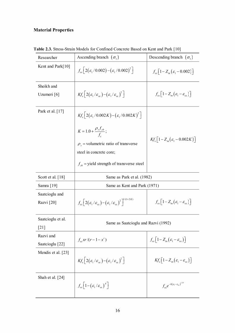
Table 2.3. Stress-Strain Models for Confined Concrete Based on Kent and Park [10]
Researcher Ascending branch ( )1σ Descending branch ( )1σ
Kent and Park[10] ( ) ( )2
cc 1 12 / 0.002 / 0.002f ε ε⎡ ⎤−⎣ ⎦ ( )cc m 11 0.002f Z ε⎡ ⎤− −⎣ ⎦
Sheikh and
Uzumeri [6] ( ) ( )2c 1 cc 1 cc2 / /Kf ε ε ε ε⎡ ⎤−⎣ ⎦ ( )cc m 1 cc1f Z ε ε⎡ ⎤− −⎣ ⎦
Park et al. [17] ( ) ( )2
c 1 12 / 0.002 / 0.002Kf K Kε ε⎡ ⎤−⎣ ⎦
c
1.0 s yhfK
fρ
= + ;
sρ = volumetric ratio of transverse
steel in concrete core;
yhf = yield strength of transverse steel
( )c m 11 0.002Kf Z Kε⎡ ⎤− −⎣ ⎦
Scott et al. [18] Same as Park et al. (1982)
Samra [19] Same as Kent and Park (1971)
Saatcioglu and
Razvi [20] ( ) ( )1/(1 2 )2
cc 1 cc 1 cc2 / /K
f ε ε ε ε+
⎡ ⎤−⎣ ⎦ ( )cc m 1 cc1f Z ε ε⎡ ⎤− −⎣ ⎦
Saatcioglu et al.
[21] Same as Saatcioglu and Razvi (1992)
Razvi and
Saatcioglu [22] cc /( 1 )rf xr r x− − ( )cc m 1 cc1f Z ε ε⎡ ⎤− −⎣ ⎦
Mendis et al. [23]
( ) ( )2c 1 cc 1 cc2 / /Kf ε ε ε ε⎡ ⎤−⎣ ⎦ ( )c m 1 cc1Kf Z ε ε⎡ ⎤− −⎣ ⎦
Shah et al. [24]
( )cc 1 cc1 / Af ε ε⎡ ⎤−⎣ ⎦ ( )1.151 cc
cckf e ε ε− −

The Mechanical Behavior and design of Composite Segment for Shield Tunnel
17
Table 2.4. Stress-Strain Models for Confined Concrete Based on Kent and Park [10]
Researcher Ascending branch ( )1σ Descending branch ( )1σ
Popovics[11] ( ) ( )c 1 co 1 co/ /( 1) / nf n nε ε ε ε⎡ ⎤− +⎣ ⎦ ; c0.058 1n f= +
Carreira and Chu[3] cc /( 1 )f xββ β× − − Mander et al.[25] cc /( 1 )rf r r x× − −
Hsu and Hsu [26] ( ) ( ){ }cc 1 cc 1 cc/ / 1 / kf k kε ε ε ε⎡ ⎤− −⎣ ⎦ 0.8( )0.5
cc0.3 dx xf e− −
Cusson and Paultre [8] cc /( 1 )f xββ β× − − 1 1 cc 2( )
cck kf e ε ε− −
Wee et al. [27]
cc /( 1 )f xββ β× − −
( )c co
11 / if E
βε
=−
21 cc /( 1 )kk f x ββ β× − −
3.0
1c
50kf
⎛ ⎞= ⎜ ⎟⎝ ⎠
;1.3
2c
50kf
⎛ ⎞= ⎜ ⎟⎝ ⎠
Hoshikuma et al.
[28]
( ) 1c 1 1 cc1 (1/ ) / nE nε ε ε −⎡ ⎤−⎣ ⎦
c cc
c cc cc
EnE f
εε
=−
( )cc des cccf E ε ε− −
desE is deterioration rate,
and can be calculated by
regression analysis of test
data in the range of ccε to
cuε
In general, we assume that the strength of confined concrete is related to the
contribution of the confinement pressure. Therefore, the strength of confined concrete
can be expressed as the sum of the strength of unconfined concrete and the strength
increase due to the confining stress. For the concrete filled steel tubular(CFST) as
shown in Fig.2.4, the core concrete and the steel tube are in a complex three
dimensional stress state, because the lateral deformation of concrete is confined by the
steel tube when CFST structures are compressed in the axial direction. Therefore, the lateral confining pressures lxf , lyf must be evaluated in the two orthogonal directions,
respectively. For the lateral confining pressure lf as shown in Fig.2.4(c) is calculated as
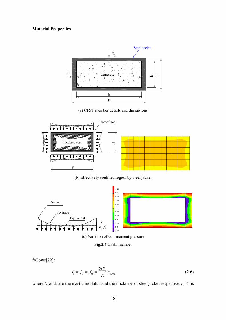
Material Properties
18
Steel jacket
Concrete
2t
1t
b
h H
B
(a) CFST member details and dimensions
Confined core
Unconfined
H
B (b) Effectively confined region by steel jacket
lf
s lk f
EquivalentAverage
Actual
(c) Variation of confinement pressure
Fig.2.4 CFST member
follows[29]:
,2 s
l lx ly h ruptEf f fD
ε= = = (2.6)
where sE andt are the elastic modulus and the thickness of steel jacket respectively, t is
The Mechanical Behavior and design of Composite Segment for Shield Tunnel
19
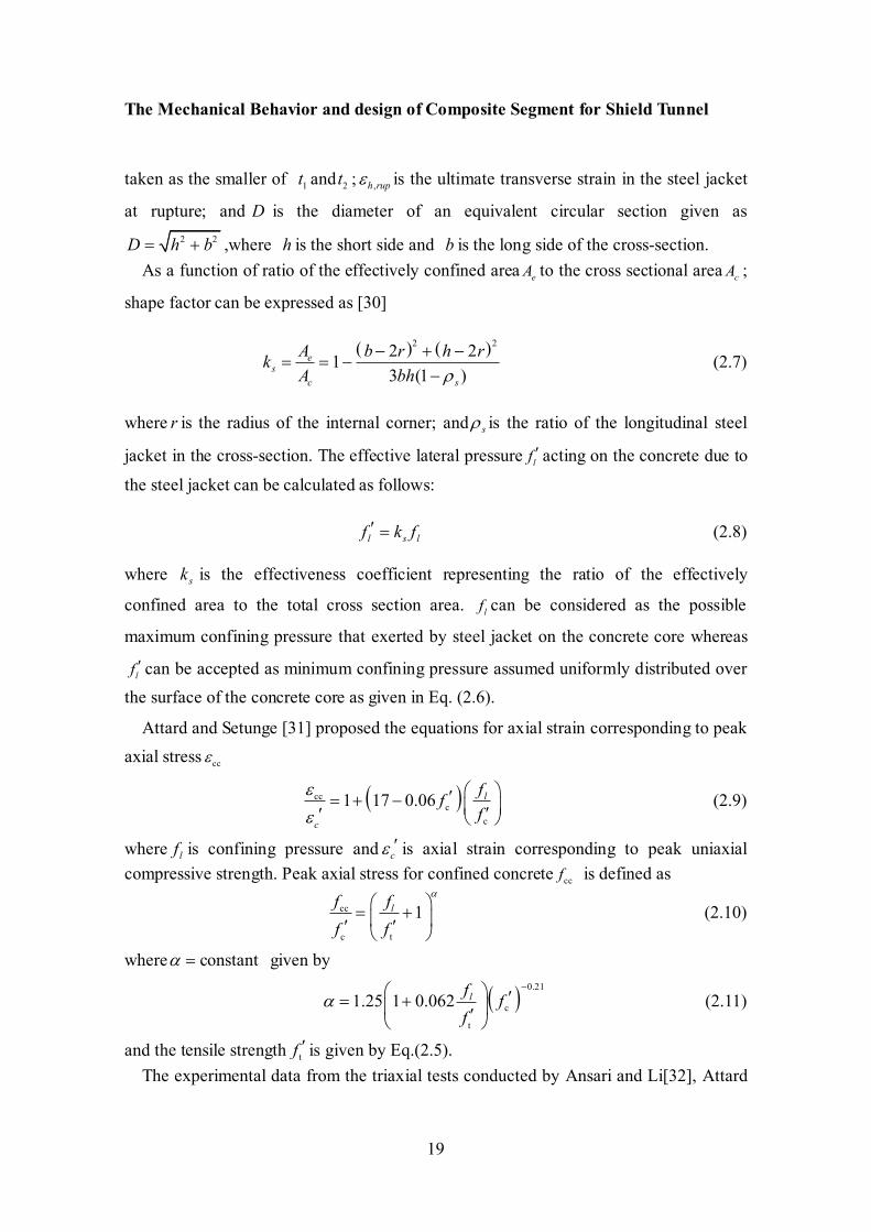
taken as the smaller of 1t and 2t ; ,h rupε is the ultimate transverse strain in the steel jacket
at rupture; and D is the diameter of an equivalent circular section given as 2 2D h b= + ,where h is the short side and b is the long side of the cross-section.
As a function of ratio of the effectively confined area eA to the cross sectional area cA ;
shape factor can be expressed as [30]
( ) ( )2 22 213 (1 )
es
c s
A b r h rkA bh ρ
− + −= = −
− (2.7)
where r is the radius of the internal corner; and sρ is the ratio of the longitudinal steel
jacket in the cross-section. The effective lateral pressure lf ′ acting on the concrete due to
the steel jacket can be calculated as follows:
l s lf k f′ = (2.8)
where sk is the effectiveness coefficient representing the ratio of the effectively
confined area to the total cross section area. lf can be considered as the possible
maximum confining pressure that exerted by steel jacket on the concrete core whereas
lf ′ can be accepted as minimum confining pressure assumed uniformly distributed over the surface of the concrete core as given in Eq. (2.6).
Attard and Setunge [31] proposed the equations for axial strain corresponding to peak axial stress ccε
( )ccc
c
1 17 0.06 l
c
fff
εε
⎛ ⎞′= + − ⎜ ⎟′′ ⎝ ⎠ (2.9)
where lf is confining pressure and cε ′ is axial strain corresponding to peak uniaxial compressive strength. Peak axial stress for confined concrete ccf is defined as
cc
c t
1lf ff f
α⎛ ⎞= +⎜ ⎟′ ′⎝ ⎠
(2.10)
where constantα = given by
( ) 0.21
c
t
1.25 1 0.062 lf ff
α−⎛ ⎞ ′= +⎜ ⎟′⎝ ⎠
(2.11)
and the tensile strength tf ′ is given by Eq.(2.5). The experimental data from the triaxial tests conducted by Ansari and Li[32], Attard
Material Properties
20
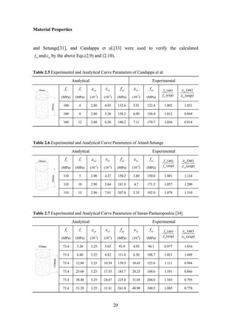
and Setunge[31], and Candappa et al.[33] were used to verify the calculated
ccf and ccε by the above Eqs.(2.9) and (2.10).
Table 2.5 Experimental and Analytical Curve Parameters of Candappa et al.
Analytical Experimental
cf
(MPa)
lf
(MPa)
coε
(10-3)
ccε
(10-3)
ccf
(MPa)
ccε
(10-3)
ccf
(MPa)
cc
cc
(an)(exp)
ff
cc
cc
(an)(exp)
εε
100 4 2.80 4.03 132.6 3.91 132.4 1.002 1.031
100 8 2.80 5.26 158.2 6.09 156.4 1.012 0.864
200m
m
98mm
100 12 2.80 6.50 180.2 7.11 170.7 1.056 0.914
Table 2.6 Experimental and Analytical Curve Parameters of Attard-Setunge
Analytical Experimental
cf
(MPa)
lf
(MPa)
coε
(10-3)
ccε
(10-3)
ccf
(MPa)
ccε
(10-3)
ccf
(MPa)
cc
cc
(an)(exp)
ff
cc
cc
(an)(exp)
εε
110 5 2.90 4.27 150.2 3.80 150.0 1.001 1.124
110 10 2.90 5.64 181.0 4.7 171.3 1.057 1.200
200m
m
100mm
110 15 2.90 7.01 207.0 5.35 192.0 1.078 1.310
Table 2.7 Experimental and Analytical Curve Parameters of Imran-Pantazopoulou [34]
Analytical Experimental
cf
(MPa)
lf
(MPa)
coε
(10-3)
ccε
(10-3)
ccf
(MPa)
ccε
(10-3)
ccf
(MPa)
cc
cc
(an)(exp)
ff
cc
cc
(an)(exp)
εε
73.4 3.20 3.25 5.03 93.9 4.95 96.1 0.977 1.016
73.4 6.40 3.25 6.82 111.0 6.50 108.7 1.021 1.049
73.4 12.80 3.25 10.39 139.5 10.45 125.6 1.111 0.994
73.4 25.60 3.25 17.53 185.7 20.25 168.6 1.101 0.866
73.4 38.40 3.25 24.67 225.0 31.05 204.0 1.103 0.795
110m
m
55mm
73.4 51.20 3.25 31.81 261.0 40.90 240.5 1.085 0.778
The Mechanical Behavior and design of Composite Segment for Shield Tunnel
21
The predictions of the confinement models agree well with the experimental data, and
are shown in Tables. 2.5, 2.6 and 2.7.
The stress-strain curve by Montoya et al.[35] was adopted to model the compressive behavior of confined concrete. The stress cσ is related to the strain cε using the
following formula:
2
1.0
ccc
c c
cc cc
f
A B Cf f
σε ε
=⎛ ⎞ ⎛ ⎞− + +⎜ ⎟ ⎜ ⎟⎝ ⎠ ⎝ ⎠
(2.12)
where dA k= ;sec
2 ABE
= ; 2sec
ACE
= ; and seccc
cc
fEε
= . The shape factor dk is given by the
following formula:
2
80
14
ccd
cc c
fkε ε⎛ ⎞= ⎜ ⎟−⎝ ⎠
(2.13)
where 80cε is the strain corresponding to 80% of the peak stress, cc0.80 f ,and given by the
following formula:
( )80 1.5 89.5 0.6 lc c c
c
fff
ε ε ⎡ ⎤′ ′= + −⎢ ⎥′⎣ ⎦ (2.14)
2.2.2 Yield and failure criterion for concrete
The Buyukozturk yield criterion [36] (adopted in MSC.MARC Code [37]) is used in
nonlinear analysis to identify the yielding condition of concrete. This criterion of
isotropic hardening and associated flow rule is developed to account for the two major
sources of nonlinearity: the progressive cracking of concrete in tension, and the
nonlinear response of concrete under multi-axial compression. Using this criterion,
incremental stress-strain relationships are established in suitable form for the nonlinear
finite element analysis.
Material Properties
22
tf ′
2σ
1σ
Com
pres
sion
Failure surface
tf
cf−
cf ′−
bcf ′−
bcf−
First yield surface
Compression-Compression zone
Compression-tension zone
Compression
Tension-tension zone
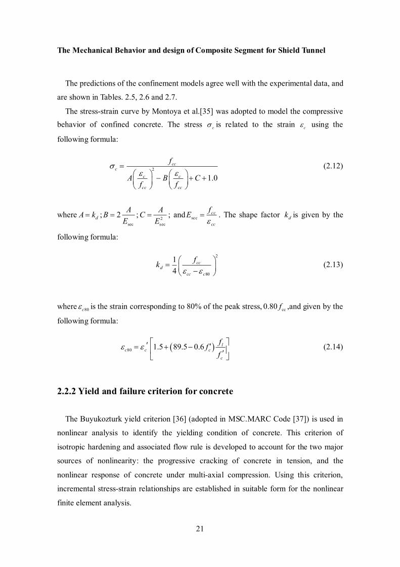
Fig.2.5 Buyukozturk yield and failure envelopes for concrete
The proposed failure criterion for concrete by Buyukozturk shown in Fig.2.5 is given
by the following formula:
2 22 0 1 1 03 3J I Iβσ α σ+ + = (2.15)
where 1I is the first invariant of stress tensor; 2J is the second invariant of stress tensor;
and β ,α and 0σ are material constants. These constants are to be determined from
the test data. For the concrete strength range used by Liu et al [38], and Kupfer et al [39], β ,α and 0σ constants were determined by a numerical trial procedure. The best fit
was found by
3β = , 1/ 5α = and 0 / 3Pσ = (2.16)
where P is uniaxial compressive strength of concrete.
2.3 Shear connectors
The bond which must be achieved between the steel element and the concrete
element in a composite member is crucial to the composite action. When the two
elements only touch at an interface such as shown in Fig. 2.6, then they are often tied
together using mechanical forms of shear connection, examples of which are given in
The Mechanical Behavior and design of Composite Segment for Shield Tunnel
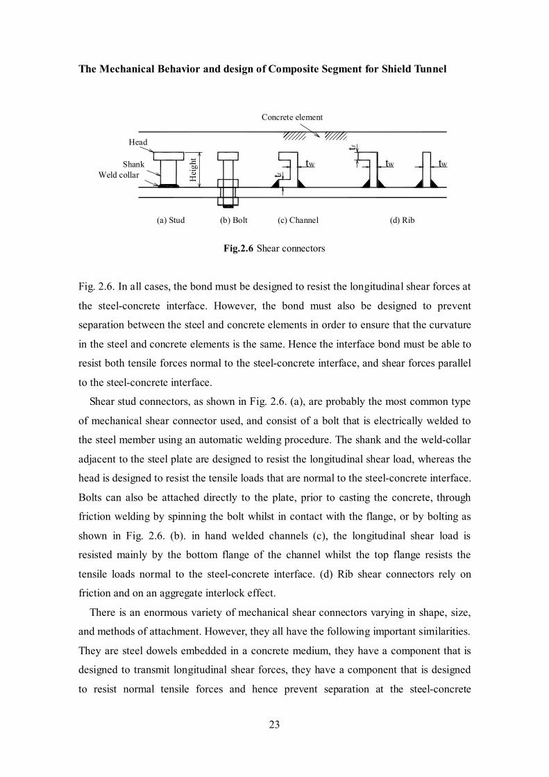
23
Head
ShankWeld collar H
eigh
t tw
(a) Stud (b) Bolt (c) Channel (d) Rib
Concrete element
tf
tw tw
tf
Fig.2.6 Shear connectors
Fig. 2.6. In all cases, the bond must be designed to resist the longitudinal shear forces at
the steel-concrete interface. However, the bond must also be designed to prevent
separation between the steel and concrete elements in order to ensure that the curvature
in the steel and concrete elements is the same. Hence the interface bond must be able to
resist both tensile forces normal to the steel-concrete interface, and shear forces parallel
to the steel-concrete interface.
Shear stud connectors, as shown in Fig. 2.6. (a), are probably the most common type
of mechanical shear connector used, and consist of a bolt that is electrically welded to
the steel member using an automatic welding procedure. The shank and the weld-collar
adjacent to the steel plate are designed to resist the longitudinal shear load, whereas the
head is designed to resist the tensile loads that are normal to the steel-concrete interface.
Bolts can also be attached directly to the plate, prior to casting the concrete, through
friction welding by spinning the bolt whilst in contact with the flange, or by bolting as
shown in Fig. 2.6. (b). in hand welded channels (c), the longitudinal shear load is
resisted mainly by the bottom flange of the channel whilst the top flange resists the
tensile loads normal to the steel-concrete interface. (d) Rib shear connectors rely on
friction and on an aggregate interlock effect.
There is an enormous variety of mechanical shear connectors varying in shape, size,
and methods of attachment. However, they all have the following important similarities.
They are steel dowels embedded in a concrete medium, they have a component that is
designed to transmit longitudinal shear forces, they have a component that is designed
to resist normal tensile forces and hence prevent separation at the steel-concrete
Material Properties
24
interface, and they all impart highly concentrated loads onto the concrete element.
In steel and concrete composite structures, the shear connectors significantly
affecting deformation and maximum carrying capacity [2], is mostly realized by means
of deformable studs [40,41], whereby steel plate to concrete infill shear occurs with
relative slip causing partial interaction [42]. This connection features limited slip
capacity and requires checking to ensure composite beam bending capacity with no
early connection failure [43]. Therefore, currently, the mechanical behavior of shear
connectors used in composite segments for shield tunnel-grouped headed stud and rib
connector will be studied in the following subsections:
2.3.1 Behavior of Shear Stud Although many researchers have investigated the static strength of the shear stud
since the 1950s, perhaps the most extensive research on the static behavior of the
headed stud was performed by Ollgaard, Slutter, and Fisher [44]. They looked at the
effect of the compressive and tensile strength, density, aggregate type, and modulus of
elasticity of the concrete, the diameter of the stud, and the number of connectors per
slab in a standard push-out test. Johnson and Molenstra [45] investigated the effect of
the strength and modulus of elasticity of stud material on the static capacity of the shear
connector and found it to be influential.
(a) Strength of Shear Stud
Many design equations have been developed to estimate the ultimate static strength
of the stud shear connectors. Different researchers have found different variables to be
influential on the static strength. Ollgaard, Slutter, and Fisher [44] proposed an equation
based on concrete properties and on the ultimate tensile strength of shear stud. Oehlers
et al [2] modified the proposed equation of shear strength by Ollgaard, Slutter, and
Fisher. They assumed concrete failure based on a 45 degrees cone, and gave the shear
strength of a shear stud in composite beam: 0.40
0.65 0.35sh
1.35.3 ( ) cu su c
s
EQ A f fEn
⎛ ⎞⎛ ⎞ ′= − ⎜ ⎟⎜ ⎟⎝ ⎠ ⎝ ⎠
(2.17)
where uQ is ultimate shear strength of a shear stud(N); n is the number of shear studs in
The Mechanical Behavior and design of Composite Segment for Shield Tunnel
25
a group; shA is the cross-sectional area of the shank of a shear stud(mm2); cf ′ is uniaxial
compressive strength of the concrete( 2N/mm ); suf is the ultimate tensile strength of a
shear stud( 2N/mm ); cE is elastic modulus of the concrete( 2N/mm ); sE is elastic modulus
of the steel( 2N/mm ).
The ultimate tensile strength of a shear stud is given by the following equation [2]:
sh sh hdsh 2
sh
( )0.642.5 cu
f h h dP A
dn
′ +⎛ ⎞= −⎜ ⎟⎝ ⎠
(2.18)
where uP is ultimate tensile strength of a shear stud(N); shh is the height of the shank of
a shear stud(mm); hdd is the diameter of the head of a shear stud(mm); shd is the diameter
of the shank of a shear stud(mm) .
(b) Load-Slip Curve
Ollgaard, Slutter, and Fisher [44] also derived an empirical expression on the
load-slip relationship for shear stud:
( )0.40.70871uQ Q e δ−= − (2.19)
where Q is the applied load(N); δ is the slip of shear stud(mm).
This equation has a vertical slope at zero load. This was observed by Ollgaard, Slutter,
and Fisher [44] in the load-slip curves due to the bond between the concrete slab and the
steel girder. However, bond at the steel-concrete interface may be lost after being
subjected to service loads for some period of time. Therefore, it is believed that Eq.
(2.19) overestimates the initial stiffness of the shear stud. The stiffness at 0.5 uQ was
proposed as initial stiffness of a shear stud by Oehlers and Bradford [2]. It can be seen
in Eq. (2.20) that the initial tangent stiffness siK increases with the cylinder strength cf ′ .
( )sh 0.16 0.0017u
si
c
QKd f
=′−
(2.20)
where siK is initial stiffness of a shear stud(N/mm)
Oehlers and Coughlan[41] derived the stiffness of the stud shear connector under
static and dynamic loads from 116 push-out test results. From the results of 42 push-out
specimens with 19 mm and 22 mm diameter shear studs, a static load-slip curve was

Material Properties
26
derived from linear regression analyses. Eq. (2.21) shows the load-slip relationship as
the ratio of the slip to the shear stud diameter.
( ) shcA B f dδ ′= + ⋅ (2.20)
The coefficients A and B are listed in Table 2.8[46]. Fig.2.7 shows load-slip
relationships for a shear stud under static loading according to Eqs.(2.19) and (2.20).
Maximum strength of the stud shear connector is assumed to be 95.9kN.
Table 2.8 Coefficients for static stiffness of a shear stud per Equation 2.20 [46]
/ uQ Q A(10-3) B(10-2) / uQ Q A(10-3) B(10-2)
0.1 22 20 0.85 138 72
0.2 40 37 0.9 156 70
0.3 52 48 0.95 223 119
0.4 63 55 0.99 319 170
0.5 80 73 1.0 371 208
0.6 102 96 1.0 406 251
0.7 120 102 0.99* 475 356
0.8 143 108 0.99* 453 178
*: Reducing loads
0.0 2.5 5.0 7.5 10.00
20
40
60
80
100
Load
(kN
)
Slip(mm)
Ollgaard et al. (1971) Oehlers and Coughlan (1986)
Fig.2.7 Load-slip curves for shear studs
The Mechanical Behavior and design of Composite Segment for Shield Tunnel
27
(c) Ultimate Slip Capacity
Oehlers and Bradford [43] gave the descending branch of the load-slip curve when
fracture of a shear stud. If fracture of a shear stud is assumed to occur when the load has reduced by 1 % from its peak, then the mean value of ults , is given by
( )ult sh0.48 0.0042 cs f d′= − (2.21)
where again the units are in N and mm. The lower 95% characteristic ultimate slip is
given by substituting 0.42 for 0.48 in Eq. (2.21). It can be seen that the slip at fracture
ults reduces as the cylinder strength cf ′ increases, and hence connectors encased in
strong concrete are less ductile than those in weak concrete, and so are more prone to
fracture. The stiffness siK and the slip ults were derived from experimental tests in
which the compressive cylinder strengths cf ′varied from 23N/mm2 to 82N/mm2.
(d) Effect of spacing on shear capacity
Shear studs are often arranged longitudinally and transversally with smaller spacing
between studs (this is referred to hereafter as the grouped arrangement). If shear studs
are grouped very closely together in the connection, the required performance may not
be satisfied. Investigations on grouped arrangement of shear studs indicated that the
strength of shear stud is different in the different grouped arrangement because of the interaction with the next shear studs. The reduction factorη proposed by Okada et al
[47] is given by
2
2
2
2
2
0.023 0.70 3 13, 25(N/mm )
0.021 0.73 3 13, 30(N/mm )
0.016 0.80 3 13, 40(N/mm )
0.013 0.84 3 13, 50(N/mm )
1 13, 25(N/mm )
l l c
l l c
l l c
l l c
l c
a a f
a a f
a a f
a a f
a f
η
⎧ ′+ ≤ < =⎪⎪ ′+ ≤ < =⎪⎪ ′= + ≤ < =⎨⎪⎪ ′+ ≤ < =⎪⎪ ′≥ ≥⎩
(2.22)
where 1 sh( / )la S d= is the longitudinal spacing factor; 1S is the longitudinal spacing of
shear studs(mm).

Material Properties
28
(e) Effect of plate thickness on shear capacity
Tests at Southampton University examined the effect of varying plate thickness and
distance between plates [48-51]. The reduction factor Vβ induced by the plate thickness
is given by
yp(0.024 0.76) and 1355V V
ftβ β= + ≤ (2.23)
where ypf is yield stress of steel plate ( 2yp 355N/mmf ≤ ), and t is thickness of steel
plate ( 10mmt ≤ ).
2.3.2 Behavior of Rib connector
The rib shear connectors (shown in Fig.2.6 (d)) can be considered as the deformed
types of the channel shear connector (shown in Fig.2.6 (c)). Therefore, the strength
calculation formula for rib shear connector can use the strength equation of channel
shear connector. The current American Standard (AISC 1993[52]) provides the
following equation for calculating the strength of a channel shear connector embedded
in a solid concrete slab:
f w r0.3( 0.5 )n c cQ t t L f E′= + (2.24)
where nQ is in Newton; ft is the flange thickness of channel shear connector(mm); wt
is the web thickness of channel shear connector(mm); and rL is the length of channel
shear connector(mm).
However, the study of Amit Pashan[53] reported that the web thickness, the area of
the channel in contact with the concrete should be considered in the calculation formula
for the strength of channel shear connector. Therefore, Amit Pashan proposed the
following equation for calculating the strength of a channel shear connector embedded
in a solid concrete slab:
2f w r w r wn c c c cQ At t f BL H f Ct L f Dt f′ ′ ′ ′= + + + (2.25)
where A, B, C, D are constants to be determined; H is Height of channel connector(mm).
The experimental results of the 18 push-out specimens with solid concrete slabs
The Mechanical Behavior and design of Composite Segment for Shield Tunnel
29
were used for the regression analysis, and yielded A, B, C, D as
A=597.058; B=5.378; C=-19.066; D=-23.672.
If the above yielded coefficients A, B, C and D are rounded to 597, 5.4, -19 and
-23.7 respectively, and substituted these values into Eq.(2.25). The final form of the
proposed equation is:
2f w r w r w597 5.4 19 23.7n c c c cQ t t f L H f t L f t f′ ′ ′ ′= + − − (2.26)
where nQ is in Newton; ft is the flange thickness of channel shear connector(mm); wt
is the web thickness of channel shear connector(mm); and rL is the length of channel
shear connector(mm); H is Height of channel connector(mm); cf ′ is uniaxial
compressive strength of concrete( 2N/mm ).
2.4. REFERENCES 1) Trahair, N.S. and Bradford, M.A., 1991. The Behaviour and Design of Steel
Structures, revised 2nd edn., Chapman and Hall, London.
2) Deric J Oehlers, Mark A Bradford, 1995: Composite steel and concrete structural
members, UK: Pergamon, Elsevier Science ,1-28.
3) Carreira, D. J., K.H. Chu,1985. Stress-strain relationship for plain concrete in
compression. J., Proc., ACI, 82(11), 797-804.
4) Wenjun, Zhang, Atsushi,Koizumi,2007. Relative slip of interface between concrete
and steel of closed-composite segment. Modern tunnelling technology. pp40-45.
5) Japan concrete committee, 2005. Standard specifications for concrete structures-2002
(structural performance verification).
6) Sheikh, S. A., and Uzumeri, S. M.,1982 . Analytical model for concrete confinement
in tied columns. J. Struct. Div. ASCE, 108 12 ,2703-2722.
7) Mander, J. B., Priestley, M. J. N., and Park, R. ,1988. Theoretical stress-strain model
for confined concrete.” J. Struct. Eng., 114(8), 1804-1826.
8) Cusson, D., and Paultre, P. ,1995. Stress–strain model for confined high strength
concrete.” J. Struct. Eng., 121(3), 468–477.
9) Sargin, M., Ghosh, S. K., and Handa, V. K. ,1971. Effects of lateral reinforcement

Material Properties
30
upon the strength and deformation properties of concrete. Mag. Concrete Res.,
23(75-76), 99-110.
10) Kent, D. C., and Park, R.,1971. Flexural members with confined concrete.J. Struct.
Div. ASCE, 97(7), 1969-1990.
11) Popovics, S., 1973. A numerical approach to the complete stress-strain curve of
concrete. Cem. Concr. Res., 3(5), 583-599.
12) Wang, P. T., Shah, S. P., and Naaman, A. E. ,1978. Stress-strain curves of normal
and lightweight concrete in compression. ACI J., 75(11),603-611.
13) Ahmad, S. H., and Shah, S. P. ,1982. Stress-strain curves of concrete confined by
spiral reinforcement.” ACI J., 79(6), 484-490.
14) El-Dash, K. M., and Ahmad, S. H. ,1995. A model for stress-strain relationship of
spirally confined normal and high-strength concrete columns. Mag. Concrete Res.,
47(171), 177-184.
15) Attard, M. M., and Setunge, S. ,1996. Stress-strain relationship of confined and
unconfined concrete. ACI Mater. J., 93(5), 432-442.
16) Assa, B., Nishiyama, M., and Watanabe, F. ,2001. New approach for modeling
confined concrete. I: Circular columns. J. Struct. Eng.,127(7), 743-750.
17) Park, R., Priestley, M. J. N., and Gill, W. D. ,1982. Ductility of square confined
concrete columns. J. Struct. Div. ASCE, 108(4), 929-950.
18) Scott, B. D., Park, R., and Priestley, N. ,1982. Stress-strain behavior of concrete
confined by overlapping hoops at low and high strain rates. ACI J., 79(1), 13-27.
19) Samra, R. M., 1990. Ductility analysis of confined columns. J. Struct. Eng., 116(11),
3148-3161.
20) Saatcioglu, M., and Razvi, S. R.,1992. Strength and ductility of confined concrete.”
J. Struct. Eng., 118(6), 1590-1607.
21) Saatcioglu, M., Salamat, A. H., and Razvi, S. R. ,1995. “Confined columns under
eccentric loading.” J. Struct. Eng., 121(11), 1547-1556.
22) Razvi, S., and Saatcioglu, M.,1999. Confinement model for high strength concrete.”
J. Struct. Eng., 125(3), 281-289.
23) Mendis, P., Pendyala, R., and Setunge, S.,2000. Stress-strain model to predict the
full-range moment curvature behavior of high-strength concrete sections.” Mag.
The Mechanical Behavior and design of Composite Segment for Shield Tunnel
31
Concrete Res., 52(4), 227-234.
24) Shah, S. P., A., and Arnold, R.,1983. Cyclic loading of spirally reinforced concrete.”
J. Struct. Eng., 109(7), 1695-1710.
25) Mander, J. B., Priestley, M. J. N., and Park, R.,1988. Observed stress-strain
behavior of confined concrete.” J. Struct. Eng., 114(8),1827-1849.
26) Hsu, L. S., and Hsu, C. T. T.,1994. Complete stress-strain behavior of high-strength
concrete under compression. Mag. Concrete Res., 46(169), 301-312.
27) Wee, T. H., Chin, M. S., and Mansur, M. A.,1996. Stress-strain relationship of high
strength concrete in compression. J. Mater. Civ.Eng., 8(2), 70-76.
28) Hoshikuma, J., Kazuhiko, K., Kazuhiko, N., and Taylor, A. W.,1996. A model for
confinement effect on stress-strain relation of reinforced concrete columns for
seismic design.” Proc., 11th World Conf. on Earthquake Engineering, Elsevier
Science, London.
29) B. Doran a, H.O. Koksal, and T. Turgay,2009. Nonlinear finite element modeling of
rectangular/square concrete columns confined with FRP. Material and design.
30) ACI Committee 440,2002. Design and construction of externally bonded FRP
systems for strengthening concrete structures (ACI 440.2R-02), Farmington Hills
(MI):American Concrete Institute.
31) Attard, M. M., and Setunge, S., 1996. Stress-strain relationship of confined and
unconfined concrete.” ACI Mater. J., 93(5), 432-442.
32) Ansari, F., and Li, Q. ,1998. High-strength concrete subjected to triaxial
compression.” ACI Mater. J., 95(6), 747-755.
33) Candappa, D. ,2000. The constitutive behavior of high strength concrete under
lateral confinement. PhD thesis, Monash Univ., Clayton,VIC, Australia.
34) Imran, I., and Pantazopoulou, S. J.,1996. Experimental study of plain concrete
under triaxial stress.” ACI Mater. J., 93(6), 589-601.
35) Montoya, E.,2003. Behavior and analysis of confined concrete. Ph.D. thesis, Univ.
of Toronto, Toronto.
36) Oral,Buyukozturk, 1977. Nonlinear analysis of reinforced concrete structure.
Computers & Structures, Vol.7, 149-156.
37) MSC.Marc Documentation, 2005. Volume A Theory and User Information. MSC
Material Properties
32
Software.
38) T. C. Y. Liu, A. H. Nilson and F. O. Slate, 1972. Stress-strain response and fracture
of concrete in uniaxial and biaxial compression. ACZ J., Proc. 69(5) 291-295.
39) H. Kupfer, H. K. Hilsdorf and H. Rusch, 1969. Behavior of concrete under biaxial
stresses. ACZ .Z. Pmt. 66(8), 656-666.
40) Ollgaard JG, Slutter RG, Fisher JW,1971. Shear strength of connectors in
lightweight and normaldensity concrete. AISC Engng, 55–64.
41) Oehlers DJ, Coughlan CG., 1986. The shear stiffness of stud shear connectors in
composite beams. J Construct Steel Res,73-84.
42) Oehlers DJ, Nguyen NT, Ahmed M, Bradford MA., 1997. Partial interaction in
composite steel and concrete beams with full shear connection. J Construct Steel
Res,41(2/3),235-48.
43) Oehlers DJ, Sved G.,1995. Composite beams with limited-slip-capacity shear
connectors. J Struct Eng.,32-38.
44) Ollgaard, J.G., Slutter, R.G., Fisher, J.W.,1971. Shear Strength of Stud Shear
Connectors in Lightweight and Normal-Weight Concrete. AISC Engineering
Journal, 8, 55-64.
45) Johnson, R.P., and Molenstra, I.N., 1991. Partial Shear Connection in Composite
Beams for Buildings. Proc. Instn Civ. Engrs, Part 2, 91, 679-704.
46) Gunup Kwon et al, 2007. Strengthening Existing Non-Composite Steel Bridge
Girders Using Post-Installed Shear Connectors. CTR Technical Report: 0-4124-1.
47) Jun,Okada,Teruhiko,Yoda, and Jean-paul, Lebet,2006. A study of the grouped
arrangements of stud connectors on shear strength behavior. Structural
Eng./Earthquake Eng.,JSCE,23(1),75-89.
48) Moy SSJ, Xiao RY, Lilistone D, 1998. Tests for British steel on the shear strength of
the studs used in the Bi-steel system. Department of Civil and Environmental
Engineering, University of Southampton.
49) Clubley SK,Moy SSJ, Xiao RY,2003. Shear strength of steel-concrete-steel
composite panels, Part I-testing and numerical modelling. Journal of
Constructional Steel Research, 59(6),781-94.
50) M. Xie, N. Foundoukosb, J.C. Chapmanb,2004. Experimental and numerical

The Mechanical Behavior and design of Composite Segment for Shield Tunnel
33
investigation on the shear behaviour of friction-welded bar–plate connections
embedded in concrete. Journal of Constructional Steel Research,61, 625-649.
51) Bowerman HG, Gough MS, King CM, 1999. Bi-steel design and construction guide.
Scunthorpe (London), British Steel Ltd.
52) AISC. 1993. Load and resistance factor design specifications for structural steel
buildings. American Institute of Steel Construction, Chicago,Illinois.
53) Amit Pashan,2006. Behaviour of channel shear connectors: Push-out tests. Master
thesis, Saskatchewan Univ., Saskatoon, Saskatchewan, Canada.

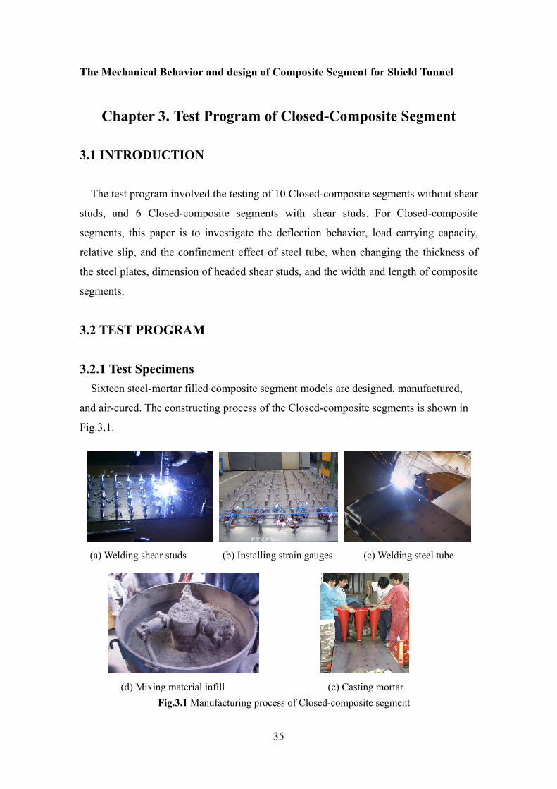
The Mechanical Behavior and design of Composite Segment for Shield Tunnel
35
Chapter 3. Test Program of Closed-Composite Segment
3.1 INTRODUCTION
The test program involved the testing of 10 Closed-composite segments without shear
studs, and 6 Closed-composite segments with shear studs. For Closed-composite
segments, this paper is to investigate the deflection behavior, load carrying capacity,
relative slip, and the confinement effect of steel tube, when changing the thickness of
the steel plates, dimension of headed shear studs, and the width and length of composite
segments.
3.2 TEST PROGRAM
3.2.1 Test Specimens
Sixteen steel-mortar filled composite segment models are designed, manufactured,
and air-cured. The constructing process of the Closed-composite segments is shown in
Fig.3.1.
(a) Welding shear studs (b) Installing strain gauges (c) Welding steel tube
(d) Mixing material infill (e) Casting mortar
Fig.3.1 Manufacturing process of Closed-composite segment
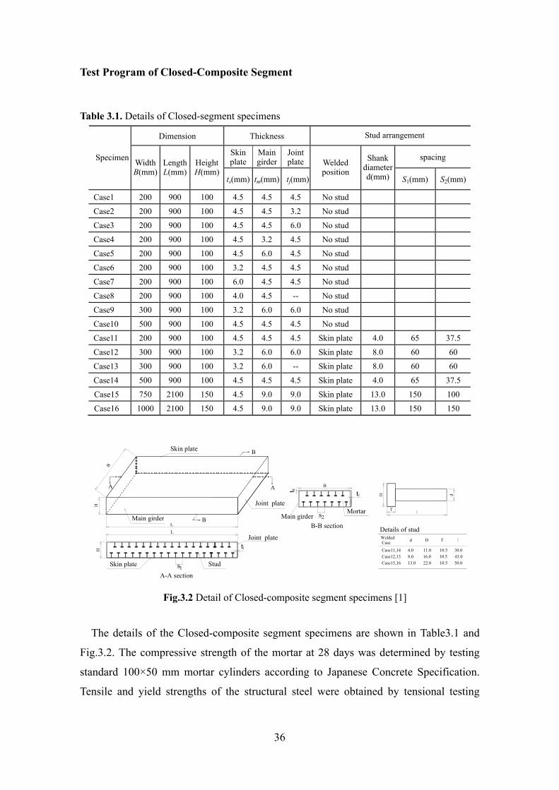
Test Program of Closed-Composite Segment
36
Table 3.1. Details of Closed-segment specimens
Dimension Thickness Stud arrangement
Skin plate
Main girder
Joint plate spacing Specimen Width
B(mm) Length L(mm)
Height H(mm)
ts(mm) tm(mm) tj(mm)
Welded position
Shankdiameterd(mm) S1(mm) S2(mm)
Case1 200 900 100 4.5 4.5 4.5 No stud
Case2 200 900 100 4.5 4.5 3.2 No stud
Case3 200 900 100 4.5 4.5 6.0 No stud
Case4 200 900 100 4.5 3.2 4.5 No stud
Case5 200 900 100 4.5 6.0 4.5 No stud
Case6 200 900 100 3.2 4.5 4.5 No stud
Case7 200 900 100 6.0 4.5 4.5 No stud
Case8 200 900 100 4.0 4.5 -- No stud
Case9 300 900 100 3.2 6.0 6.0 No stud
Case10 500 900 100 4.5 4.5 4.5 No stud
Case11 200 900 100 4.5 4.5 4.5 Skin plate 4.0 65 37.5
Case12 300 900 100 3.2 6.0 6.0 Skin plate 8.0 60 60
Case13 300 900 100 3.2 6.0 -- Skin plate 8.0 60 60
Case14 500 900 100 4.5 4.5 4.5 Skin plate 4.0 65 37.5
Case15 750 2100 150 4.5 9.0 9.0 Skin plate 13.0 150 100
Case16 1000 2100 150 4.5 9.0 9.0 Skin plate 13.0 150 150
B
t s tj
s2
B
H
L
Skin plate
L
H
tj
s1
AA
B
B
A-A section
B-B section
Joint plate
Joint plate
Main girder
Skin plate Stud
Main girderMortar T
dD
Details of studWelded Case d D T
Case11,14 Case12,13 Case15,16
4.08.0
13.0
11.016.0 22.0
10.510.5 10.5
30.043.0
50.0
Fig.3.2 Detail of Closed-composite segment specimens [1]
The details of the Closed-composite segment specimens are shown in Table3.1 and
Fig.3.2. The compressive strength of the mortar at 28 days was determined by testing
standard 100×50 mm mortar cylinders according to Japanese Concrete Specification.
Tensile and yield strengths of the structural steel were obtained by tensional testing

The Mechanical Behavior and design of Composite Segment for Shield Tunnel
37
according to Japanese Structural Steel Specification. Mechanical properties of structural
steel (SS400) and mortar are shown in Table 3.2. The mix proportions of the mortar are
as follows: Cement: 666.7 kg/m3; Water: 266.7 kg/m3; Sand: 1333.3 kg/m3 (size: 5mm);
Cement/Water ratio: 40%; Water-reducing admixture: 666.7 cc/m3; Polymer dispersion:
2.22 kg/m3.
Table 3.2. Mechanical material properties for Closed-composite segment specimens
Structural steel (SS400) Mortar
Specimen Yield strength
2(N/mm )yf
Tensile strength
2(N/mm )sf ′
Young modulus
2(N/mm )sE
Compressive strength
2(N/mm )cf ′
Young modulus
2(N/mm )cE
Case1 325 448 2.0×10⁵ 52.3 2.41×10⁴
Case2 325 448 2.0×10⁵ 52.3 2.41×10⁴
Case3 325 448 2.0×10⁵ 52.3 2.41×10⁴
Case4 325 448 2.0×10⁵ 52.3 2.41×10⁴
Case5 325 448 2.0×10⁵ 52.3 2.41×10⁴
Case6 325 448 2.0×10⁵ 52.3 2.41×10⁴
Case7 325 448 2.0×10⁵ 52.3 2.41×10⁴
Case8 325 448 2.0×10⁵ 52.3 2.41×10⁴
Case9 333 423 2.05×10⁵ 86.8 2.85×10⁴
Case10 303 430 2.25×10⁵ 73.5 2.36×10⁴
Case11 325 448 2.0×10⁵ 52.3 2.41×10⁴
Case12 333 423 2.05×10⁵ 86.8 2.85×10⁴
Case13 333 423 2.05×10⁵ 86.8 2.85×10⁴
Case14 303 430 2.25×10⁵ 73.5 2.36×10⁴
Case15 328 457 1.95×10⁵ 77.6 2.57×10⁴
Case16 328 457 1.95×10⁵ 77.6 2.57×10⁴
3.2.2 Test Setup
The simply supported Closed-composite segment specimens were loaded
symmetrically at four points within the span using a spreader beam. In these test
arrangements, such loading led, in theory, pure bending between applied forces of the
composite segment specimens can be obtained between the two loading points without
the presence of shear and axial forces. The Biaxial Structure Test Machine shown in Fig.
3.3 of 5000kN capability was used to apply monotonic load. The test specimens of

Test Program of Closed-Composite Segment
38
Case1 to Case8 were designed to study the effects of the thickness of the steel plates
changing on load carrying capacity; The test specimens of Case9 to Case14 were
designed to study the behavior of composite segments with/without shear studs; Case15,
Case16 were designed to study the interface relative slip between the skin plates and the
mortar infill shown in Fig.3.4. The applied load was measured and recorded using a
load cell. The loads were increased gradually with an increment of approximately 5kN
until the ultimate carrying capacities of Case1 to Case8, Case10, Case11, and Case13.
However, for Case9, Case12 to Case16, initial loading control was based on readings of
the load applied through the load cell, until the load-deflection response became
non-linear. Thereafter, loading was shifted to displacement control based on increments
of midspan deflection, until failure of the specimen was observed or until very large
deflections occurred. Resistance strain gauges were fixed to the inside/outside of the
steel tube and mortar infill. Finally, all the data records were made on data logger (data
acquisition equipment). Displacement transducers and Strain gauges located on key
points shown in Fig.3.5 and Fig.3.6 were used to measure strains and deflections
respectively.
(a) Biaxial Structure Test Machine (c) Data logger
Fig. 3.3 Biaxial Structure Test Machine and measuring instruments
(b) Switch box
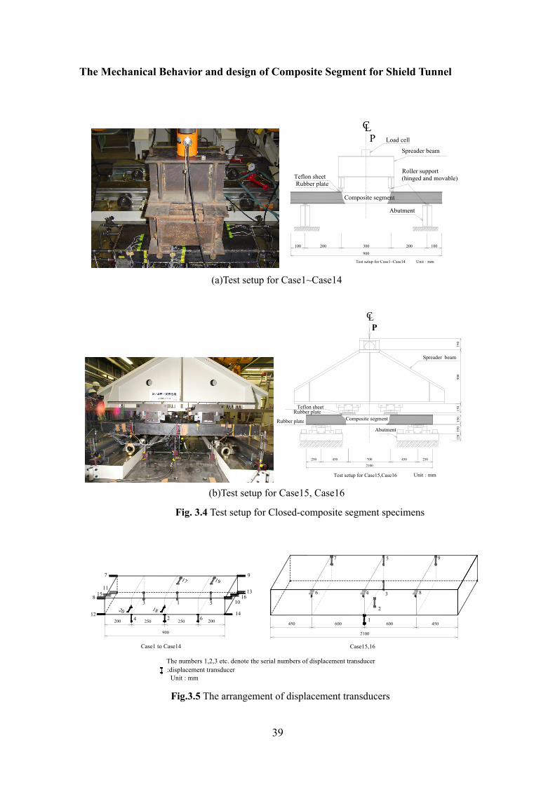
The Mechanical Behavior and design of Composite Segment for Shield Tunnel
39
The numbers 1,2,3 etc. denote the serial numbers of displacement transducer :displacement transducer Unit : mm
Case15,16
204 2 6
14
1016
13
91917
7
11158
12
3 1 518
200 250 250 200 1
3
2
6 4
450 600
2100
8
7
600
95
450
Case1 to Case14
900
Fig.3.5 The arrangement of displacement transducers
100 200 300 200 100
900
CL
Composite segment
Abutment
Spreader beam
Load cell
Teflon sheetRubber plate
P
Unit:mmTest setup for Case1~Case14
Roller support(hinged and movable)
(a)Test setup for Case1~Case14
Composite segment
2100
700
Unit:mm
LC
120
150
150
900
190
150
P
450250 250450
AbutmentRubber plate
Teflon sheetRubber plate
Spreader beam
Test setup for Case15,Case16
(b)Test setup for Case15, Case16
Fig. 3.4 Test setup for Closed-composite segment specimens
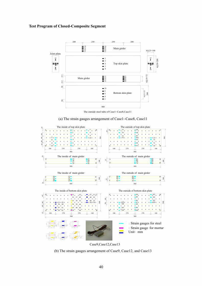
Test Program of Closed-Composite Segment
40
4@25=100
4@33
=122
4@18
=72
3434
18.5
4@50
=200
18.5
200
900
35
1
13151719 30
242628
42
6
252321
2729
1216141820
39
41
40
383752
810
11 22
79
33
35 313236
34
200 250 250 200
Top skin plate
Bottom skin plate
Main girder
Main girder
The outside steel tube of Case1~Case8,Case11
Joint plate
(a) The strain gauges arrangement of Case1~Case8, Case11
1112
1314
3
56
4
12
7
8
910
7776
7574
6463
6665
67
68
69
7071
7372
15161718 26
252423
30292827
22212019
90919293
82838485
81807978
89888786
105106
107108
9495
969798
99100
104103
10210131
32
33
34
3536
39
40
37
385960
6162
5556
5758
44
4546
42
43
41
The inside of top skin plateA
D C
B D
A B
C
A B
C D
C D
A B
C'
B'A'
D' B'
C'D'
A'48 52
54505349
5147
900
180 270 270 180
300
100
900
900
180 270 270 180
300
1545
60
45
6060
888
A' B'
A' B'
888 888
C' D'
C' D'
900
180 270 270 180
300
900
180 270 270 180
300
1545
6060
6030
1010
2737
Case9,Case12,Case13
The outside of top skin plate
The inside of main girder The outside of main girder
The inside of main girder The outside of main girder
100
100
100
The inside of bottom skin plate The outside of bottom skin plate
:Strain gauges for steel : Strain gauge for mortar Unit: mm
(b) The strain gauges arrangement of Case9, Case12, and Case13
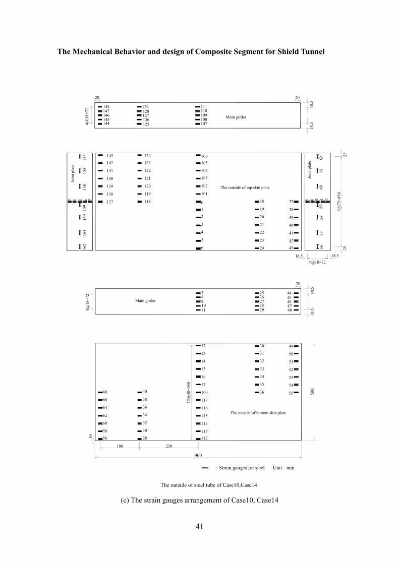
The Mechanical Behavior and design of Composite Segment for Shield Tunnel
41
106105
103
102
101
012
3
4
5
6
143
142
141
140
139
138
137
124123
122
121
120
119
118 18
19
20
21
22
23
24
37
38
39
40
41
4243
63 64 65 66 67
109
107
111110
108
129
127
125
128
126
148
146
144145
147
165 164 163167 166
7
9
11
8
10
25
27
29
26
28
44
46
48
45
47
68
66
64
62
60
58
56
40
38
36
34
32
30
28
12
13
14
15
16
17
100
117
116
115
114
113112
30
31
32
33
34
35
36
49
50
51
52
53
54
55
156
155
158
159
160
161
162
6162
6059
5857
56
4@18
=72 18
.518
.5
12@
40=4
80
6@75
=450
2525
4@18=7218.5 18.5
180 250
500
900
104
10
20 20
The outside of steel tube of Case10,Case14
Main girder
The outside of top skin plate
The outside of bottom skin plate
Main girder
Join
t pla
te
Join
t pla
te18
.518
.5
20
4@18
=72
:Strain gauges for steel Unit: mm
(c) The strain gauges arrangement of Case10, Case14
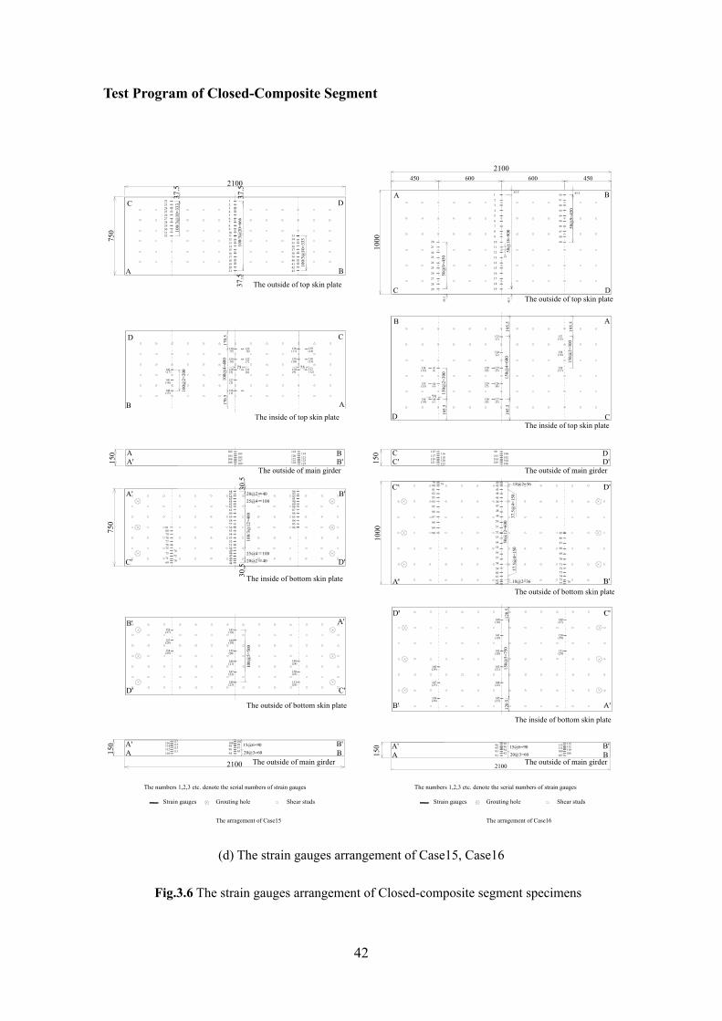
Test Program of Closed-Composite Segment
42
A B
C D
C' D'
A' B'
50@
18=9
00
45.5
50@
9=45
045
.5
50@
9=45
0
45.5
50@
12=6
00
37.5
@4=
150
37.5
@4=
150
18@2=36
18@2=36
25
30
31
32
33
34
35
36
37
38
39
450 600 600 4502100
D'
B'
146(24)
147(25)
148(26)
D
B
195.
515
0@2=
300
134(12)
135(13)
136(14)
131(9)
132(10)
133(11)
75
120.
5 C'140(18)
141(19)
142(20)
143(21)
144(22)
145(23)
120.
515
0@5=
750
149(27)
150(28)
151(29)
A'
137(15)
138(16)
139(17)
123(1)
124(2)
125(3)
126(4)
127(5)
128(6)
129(7)
130(8)
195.
515
0@4=
600
195.
5
150@
2=30
0
C
A
195.
5
2100
AA'
C'C
15@6=90
20@3=60 BB'
D'D
The numbers 1,2,3 etc. denote the serial numbers of strain gauges
1000
150
1000
150
45.5
20
21
2223
24
25
26
27
28
29
1
2
3
4
5
6
7
8
9
10
11
12
13
14
15
16
17
18
19
115117119121
116118120122
99101103105
100102104106
8081
838485
86
87
88
89
90
78 79
82
4243
464748
49
50
51
52
53
40
45
5455
56
57
58
5960616264
65
6667
68
69
70
717273747577
44
76
9593
9291
949696 98
111109
108107
110112113 114
The outside of top skin plate
The inside of top skin plate
The outside of main girder
The outside of bottom skin plate
The inside of bottom skin plate
The outside of main girder
Strain gauges Grouting hole Shear studs
The arragement of Case16
D'
B'
B
149(24)
150(25)
151(26)
D
100@
2=20
0
139(14)
138(13)
137(12)
142(17)
141(16)
140(15)
170.
5
152(27)
153(28)
154(29)
143(18)
144(19)
145(20)
146(21)
147(22)
148(23)
100@
5=50
0
C'
A'
A
130(5)
129(4)
128(3)
127(2)
126(1)
100@
4=40
0
133(8)
132(7)
131(6)
170.
5
136(11)
135(10)
134(9)
C
A
750
C'
750
A'
C
100/
3@10
=333
20@2=4025@4=100
100/
3@12
=400
20@2=4025@4=100
D'
B'
B
100/
3@20
=666
100/
3@10
=333
D2223242526272829303132
2100
123456789101112131415161718192021
37.5
37.5
37.5
34353637383940414243
33
75 75
A'A
B'B
150 118
120122124
119121123125
102104106108
103105107109
2100AA' 15@6=90
20@3=60 BB'
150 98
9695
94
9799100 101
114112
111110
113115116 117
69 70
73
75
77
798081
76
78
7172
74
4445
48
50
52
545556
51
53
4647
49
5758
63
65
6768
6466
59
626160
868584
89
91
9394
9092
85
888786
30.5
30.5
The outside of main girder
The inside of bottom skin plate
The outside of bottom skin plate
The outside of main girder
The inside of top skin plate
The outside of top skin plate
The numbers 1,2,3 etc. denote the serial numbers of strain gauges
Strain gauges Grouting hole Shear studs
The arragement of Case15
(d) The strain gauges arrangement of Case15, Case16
Fig.3.6 The strain gauges arrangement of Closed-composite segment specimens
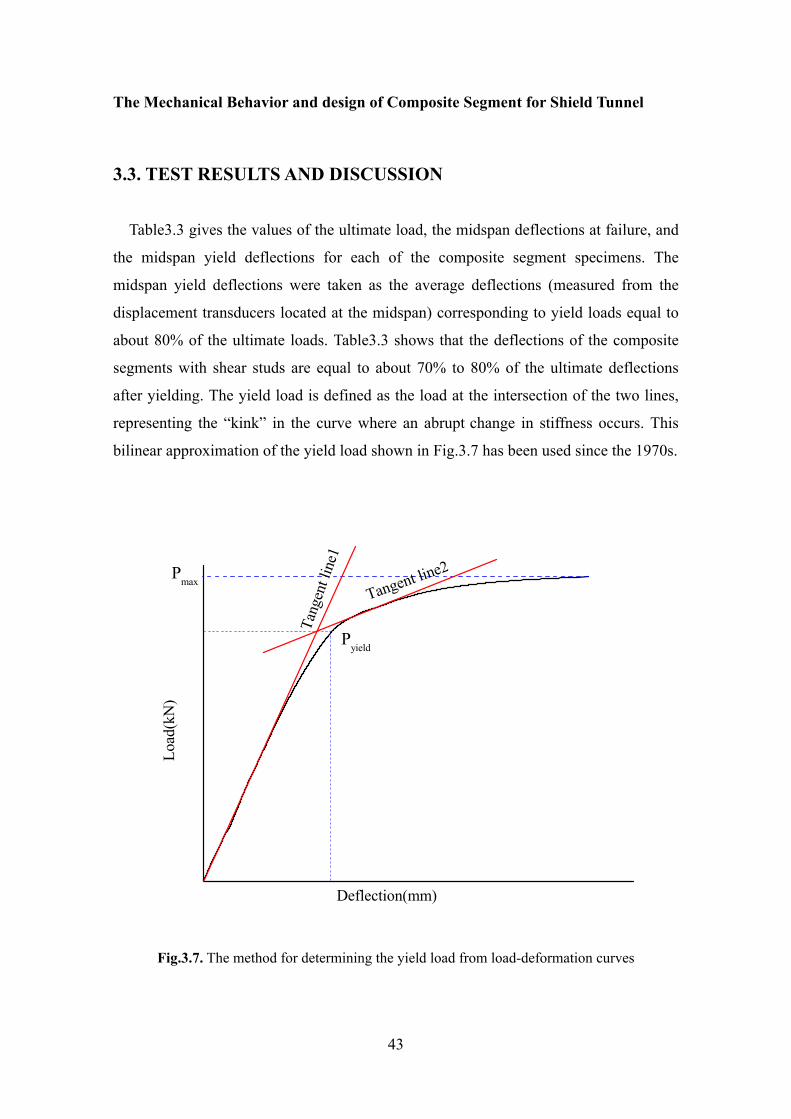
The Mechanical Behavior and design of Composite Segment for Shield Tunnel
43
3.3. TEST RESULTS AND DISCUSSION
Table3.3 gives the values of the ultimate load, the midspan deflections at failure, and
the midspan yield deflections for each of the composite segment specimens. The
midspan yield deflections were taken as the average deflections (measured from the
displacement transducers located at the midspan) corresponding to yield loads equal to
about 80% of the ultimate loads. Table3.3 shows that the deflections of the composite
segments with shear studs are equal to about 70% to 80% of the ultimate deflections
after yielding. The yield load is defined as the load at the intersection of the two lines,
representing the “kink” in the curve where an abrupt change in stiffness occurs. This
bilinear approximation of the yield load shown in Fig.3.7 has been used since the 1970s.
Deflection(mm)
Pmax
Tang
ent l
ine1
Tangent line2
Pyield
Load
(kN
)
Fig.3.7. The method for determining the yield load from load-deformation curves

Test Program of Closed-Composite Segment
44
Table 3.3. Experimental results of Closed-composite segment specimens
Specimen Yield load(kN)
Ultimate load (kN)
Yield load /Ultimate load
(%)
Yield deflection
yδ (mm)
Deflection at failure uδ (mm)
( ) /u y uδ δ δ−
(%)
Case1 380 470 80.9 3.35 8.19 59.1
Case2 375 450 83.3 3.50 7.39 52.6
Case3 380 470 80.9 3.35 9.62 65.2
Case4 315 425 74.1 3.0 8.74 65.7
Case5 415 500 83.0 3.49 9.31 62.5
Case6 298 370 80.5 3.16 7.78 59.3
Case7 410 530 77.4 3.28 10.74 69.5
Case8 260 345 75.4 2.87 10.87 73.6
Case9 250 380 65.7 2.88 16.6 82.7
Case10 570 705 80.9 3.9 13.0 70.0
Case11 400 505 79.2 3.01 11.3 73.4
Case12 352 427 82.4 3.89 27.9 86.1
Case13 304 425 71.6 3.53 20.4 82.7
Case14 620 790 78.5 3.52 20.2 82.6
Case15 1000 1222 81.8 10.48 35.7 70.6
Case16 1244 1533 81.1 12.06 39.1 69.2
3.3.1 Load-Deflection Response
Load and midspan deflection relationships for all tested specimens can be described
by the load-midspan deflection curves shown in Fig.3.8. It can be observed that the
load-midspan deflection curves are linear up to a load corresponding to the yield point.
After yielding, composite segments with shear studs represents very large deflection or
excellent ductility, and maintain load carrying capacity to achieve the ultimate
deflection. Fig.3.8 (a) shows the effect of thickness of steel tube on load carrying

The Mechanical Behavior and design of Composite Segment for Shield Tunnel
45
capacity. It can be observed that the thickness of steel tube markedly affect the load
carrying capacities of the composite segments. Fig.3.8 (b), (c), and (d) show the effect
of shear studs on load carrying capacity. It can be observed that the load carrying
capacities of the composite segments with shear studs are larger than those of the
composite segments without shear studs, and composite structural members show
differently the degree of shear connection. From Fig.8 (e), it can be observed that the
joint plates as shear connectors markedly affect the load carrying capacities of the
composite segments without shear studs. However, the joint plates only affect the
deflection of the range from yield load to ultimate load, and not affect the load carrying
capacities of the composite segments with shear studs shown in Fig.8 (f). It can be
concluded that joint plate should be considered as shear connectors, and resist the shear
force occurring in the interface between steel tube and concrete infill with shear studs in
ultimate limit analysis.
0 2 4 6 8 10 120
50
100
150
200
250
300
350
400
450
500
550
Case3
Case2
Case1
Case6
Case4
Case5Case7
Load
(kN
)
Deflection at midspan(mm)
Yield pointCase1 (3.35,380)Case2 (3.50,375)Case3 (3.35,380)Case4 (3.00,315)Case5 (3.49,415)Case6 (3.16,298)Case7 (3.28,410)
(a) Load-deflection curves for Case1~Case7 without shear studs
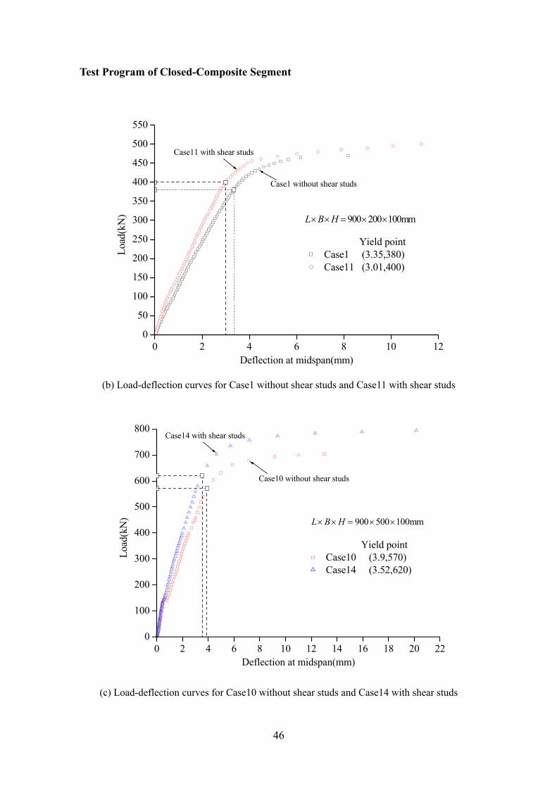
Test Program of Closed-Composite Segment
46
0 2 4 6 8 10 120
50
100
150
200
250
300
350
400
450
500
550
900 200 100mmL B H× × = × ×
Case1 without shear studs
Case11 with shear studs
Load
(kN
)
Deflection at midspan(mm)
Yield pointCase1 (3.35,380)Case11 (3.01,400)
(b) Load-deflection curves for Case1 without shear studs and Case11 with shear studs
0 2 4 6 8 10 12 14 16 18 20 220
100
200
300
400
500
600
700
800
900 500 100mmL B H× × = × ×
Case10 without shear studs
Case14 with shear studs
Load
(kN
)
Deflection at midspan(mm)
Yield pointCase10 (3.9,570)Case14 (3.52,620)
(c) Load-deflection curves for Case10 without shear studs and Case14 with shear studs
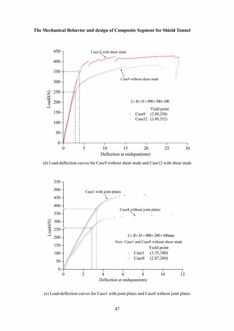
The Mechanical Behavior and design of Composite Segment for Shield Tunnel
47
0 5 10 15 20 25 300
50
100
150
200
250
300
350
400
450
900 300 100L B H× × = × ×
Case9 without shear studs
Case12 with shear studsLo
ad(k
N)
Deflection at midspan(mm)
Yield pointCase9 (2.88,250)Case12 (3.89,352)
(d) Load-deflection curves for Case9 without shear studs and Case12 with shear studs
0 2 4 6 8 10 120
50
100
150
200
250
300
350
400
450
500
550
900 200 100mmL B H× × = × ×Note: Case1 and Case8 without shear studs
Case1 with joint plates
Case8 without joint plates
Load
(kN
)
Deflection at midspan(mm)
Yield pointCase1 (3.35,380)Case8 (2.87,260)
(e) Load-deflection curves for Case1 with joint plates and Case8 without joint plates
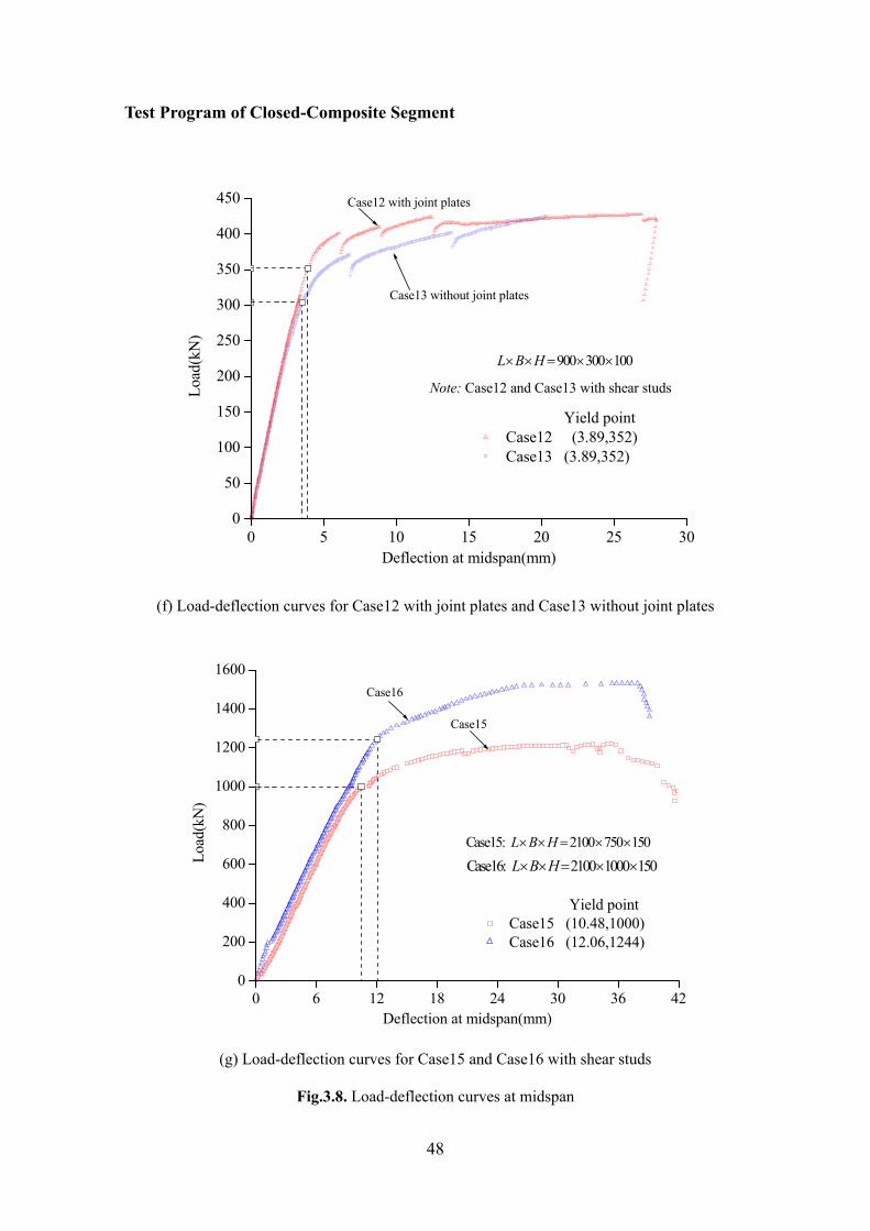
Test Program of Closed-Composite Segment
48
0 5 10 15 20 25 300
50
100
150
200
250
300
350
400
450
Note: Case12 and Case13 with shear studs
900 300 100L B H× × = × ×
Case13 without joint plates
Case12 with joint platesLo
ad(k
N)
Deflection at midspan(mm)
Yield pointCase12 (3.89,352)Case13 (3.89,352)
(f) Load-deflection curves for Case12 with joint plates and Case13 without joint plates
0 6 12 18 24 30 36 420
200
400
600
800
1000
1200
1400
1600
Case16: 2100 1000 150L B H× × = × ×
Case15: 2100 750 150L B H× × = × ×
Case15
Case16
Load
(kN
)
Deflection at midspan(mm)
Yield pointCase15 (10.48,1000)Case16 (12.06,1244)
(g) Load-deflection curves for Case15 and Case16 with shear studs
Fig.3.8. Load-deflection curves at midspan

The Mechanical Behavior and design of Composite Segment for Shield Tunnel
49
3.3.2 Strain Distribution
Fig.3.9 shows the measured strain distribution along the composite segment width
(with the origin at the center of the top skin plates) on the surfaces of the skin plates and
main girders. Such curves are displayed under different loading levels for the midspan
sections of the composite segment specimens. In general, the strain values on the
surfaces of the skin plates of the composite segments without shear studs are larger than
those of the composite segments with shear studs (Fig.3.9(a), (b)), and the top skin plate
of the composite segment without shear studs appears the local buckling(the strain
values on the surfaces of the top skin plate shift from negative to positive), it can be
concluded that no shear connection is provided between the mortar infill and the steel
plates, and the two components work independently resisting the moment. It is observed
from Fig.3.9(c) that the strain values on the skin plates increase and decrease repeatedly,
and the strain distribution shows markedly wavy change with increasing load. The strain
response is attributed to the shear lag effect of shear studs embedded in the skin plates.
Some values of the strains in the skin plates are larger than the values of the strains on
the edges of the main girders. The confinement effect of the main girders
on the deflection of the skin plates is greater. Based on testing investigation, it can be
-420 -350 -280 -210 -140 -70 0 70 140 210 280 350 420
-2000
-1500
-1000
-500
0
500
1000
1500
2000
Stud position
200kN
150kN
100kN
Bottom skin plateGirderBottom skin plate Girder
(mm)Distance from the middle of the width of the top skin plate
Top skin plate
Mic
rostr
ain
Case9 Case12 Case9 Case12 Case9 Case12
(a) Measured strain distribution on the surfaces of steel plates along the midspan section for
Case9 without shear studs and Case12 with shear studs

Test Program of Closed-Composite Segment
50
-630 -540 -450 -360 -270 -180 -90 0 90 180 270 360 450 540 630
-1500
-1200
-900
-600
-300
0
300
600
900
1200
1500
Stud position
400kN
200kN
100kN
Bottom skin plateGirderBottom skin plate Girder
(mm)Distance from the middle of the width of the top skin plate
Top skin plate
Mic
rostr
ain
Case10 Case14 Case10 Case14 Case10 Case14
(b) Measured strain distribution on the surfaces of steel plates along the midspan section for
Case10 without shear studs and Case14 with shear studs
-900 -600 -300 0 300 600 900
-1500
-1000
-500
0
500
1000
1500
Bottom skin plateGirderBottom skin plate GirderStud position
(mm)Distance from the middle of the width of the top skin plate
Top skin plate
Mic
rost
rain
Case15 40kN 200kN 400kN 600kN
(c) Measured strain distribution on the surfaces of steel plates along the midspan section for
Case15 with shear studs Fig.3.9. Measured strain distribution on the surfaces of steel plates along the midspan section
observed that the shear studs and the main girders can affect not only the overall
response (e.g., shape of the load-deflection curve), but also local results (e.g., strain
distributions along the skin plates).
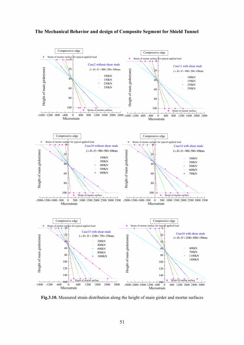
The Mechanical Behavior and design of Composite Segment for Shield Tunnel
51
-1600 -1200 -800 -400 0 400 800 1200 1600 2000 2400
100
80
60
40
20
0 Strain of mortar surface for typical applied load
Strain of mortar surface
Case2 without shear studs900 200 100mmL B H× × = × ×
100kN 150kN 250kN 350kN
Hei
ght o
f mai
n gi
rder
(mm
)
Compressive edge
Microstrain
-1600 -1200 -800 -400 0 400 800 1200 1600 2000 2400
100
80
60
40
20
0 Strain of mortar surface for typical applied load
Strain of mortar surface
Case11 with shear studs900 200 100mmL B H× × = × ×
100kN 150kN 250kN 350kN
Hei
ght o
f mai
n gi
rder
(mm
)
Compressive edge
Microstrain
-2000-1500-1000 -500 0 500 1000 1500 2000 2500 3000 3500
100
80
60
40
20
0
100kN 300kN 400kN 500kN 600kN
Strain of mortar surface
Strain of mortar surface for typical applied load
900 500 100mmL B H× × = × ×
Case10 without shear studs
Hei
ght o
f mai
n gi
rder
(mm
)
Compressive edge
Microstrain
-2000-1500-1000 -500 0 500 1000 1500 2000 2500 3000 3500
100
80
60
40
20
0
Strain of mortar surface
Strain of mortar surface for typical applied load
900 500 100mmL B H× × = × ×
100kN 300kN 500kN 600kN 700kN
Case14 with shear studs
Hei
ght o
f mai
n gi
rder
(mm
)
Compressive edge
Microstrain
-1800 -1200 -600 0 600 1200 1800 2400 3000160
140
120
100
80
60
40
20
0
Strain of mortar surface
Strain of mortar surface for typical applied load
Case15 with shear studs2100 750 150mmL B H× × = × ×
Hei
ght o
f mai
n gi
rder
(mm
)
Compressive edge
Microstrain
200kN 400kN 600kN 800kN 1000kN
-3000-2400-1800-1200 -600 0 600 1200 1800 2400 3000160
140
120
100
80
60
40
20
0
Strain of mortar surface
Strain of mortar surface for typical applied load
2100 1000 150mmL B H× × = × ×
400kN 700kN 1100kN 1400kN
Case16 with shear studs
Hei
ght o
f mai
n gi
rder
(mm
)
Compressive edge
Microstrain
Fig.3.10. Measured strain distribution along the height of main girder and mortar surfaces
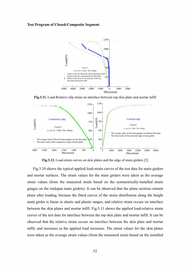
Test Program of Closed-Composite Segment
52
-5000 -4000 -3000 -2000 -1000 0 1000 20000
250
500
750
1000
1250
2100 750 150mmL B H× × = × ×
Case15Lo
ad(k
N)
Microstrain
Strain on the top skin plate contacting mortar infill Strain on mortar contacting the top skin plate Relative slip strain on the interface of the top
skin plate and mortar infill
Fig.3.11. Load-Relative slip strain on interface between top skin plate and mortar infill
-3000 -2500 -2000 -1500 -1000 -500 00
250
500
750
1000
1250
Compressive edge
2100 750 150mmL B H× × = × ×
Case15
Microstrain
Load
(kN
)
The average value of the all strain gauages on top skin plate The strain value of the compressive edge of main girder
0 3000 6000 9000 12000 15000 180000
250
500
750
1000
1250
Tensional edge
2100 750 150mmL B H× × = × ×
Case15
The average value of all strain gauages on bottom skin plate The strain value of the tensional edge of main girder
Microstrain
Load
(kN
)
Fig.3.12. Load-strain curves on skin plates and the edge of main girders [2]
Fig.3.10 shows the typical applied load-strain curves of the test data for main girders
and mortar surfaces. The strain values for the main girders were taken as the average
strain values (from the measured strain based on the symmetrically-installed strain
gauges on the midspan main girders). It can be observed that the plane sections remain
plane after loading, because the fitted curves of the strain distribution along the height
main girder is linear in elastic and plastic ranges, and relative strain occurs on interface
between the skin plates and mortar infill. Fig.3.11 shows the applied load-relative strain
curves of the test data for interface between the top skin plate and mortar infill. It can be
observed that the relative strain occurs on interface between the skin plate and mortar
infill, and increases as the applied load increases. The strain values for the skin plates
were taken as the average strain values (from the measured strain based on the installed

The Mechanical Behavior and design of Composite Segment for Shield Tunnel
53
strain gauges on the inside and outside of skin plates along the width of the specimen)
shown in Fig.3.12. The strain values of the edges of main girders are about equal to the
average values of the skin plate. Therefore, it can be concluded that the shear studs
installed in compressive and tensional sides resist the compressive resultant force
occurring on the compressive main girder and top skin plate, and on the tensional
resultant force occurring on the tensional main girder and bottom skin plate,
respectively.
3.3.3 Sensitivity Study
An investigation was performed to evaluate the sensitivity of the overall response of
Closed-composite segments (represented by ultimate loads) to likely variations in the
thicknesses of the steel plates. Composite segment specimens of Case1 to Case7 without
shear studs described in Table3.1 were used for the sensitivity study. The dimension of
the compared standard case (Case1) is L×W×H = 900×200×100 mm; all the thicknesses
of skin plates, main girders, and joint plates are 4.5 mm. If the ratios of ultimate
carrying capacity are defined as the ratios of the ultimate carrying capacities of Case2,
Case3, etc to the ultimate carrying capacity of Case1, the relationship of the ratio of
ultimate carrying capacity and percentage change of the thicknesses of the steel plates is
shown in Fig.3.13. It can be observed that the thicknesses of the skin plates obviously
affect the ultimate carrying capacities of the Closed-composite segments.
70 80 90 100 110 120 130 1400.6
0.8
1.0
1.2
The ultimate carrying capacity of Case2~Case7ui :PThe ultimate carrying capacity of standard case(Case1)us :P
(%) :ρ
ui
us
(%) ( 2,3,4,5,6,7)P iP
ρ = =
Ratio of the ultimate carrying capacity(%)
Rat
io o
f ulti
mat
e ca
rryi
ng c
apac
ity
Percentage change of the thicknesses of steel plates(%)
Thicknesses of skin plates Thicknesses of main girders Thicknesses of joint plates
Fig.3.13. Effects of the changing thicknesses of steel tube on ultimate carrying capacity
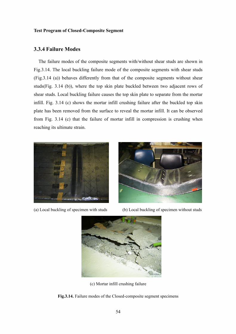
Test Program of Closed-Composite Segment
54
3.3.4 Failure Modes
The failure modes of the composite segments with/without shear studs are shown in
Fig.3.14. The local buckling failure mode of the composite segments with shear studs
(Fig.3.14 (a)) behaves differently from that of the composite segments without shear
studs(Fig. 3.14 (b)), where the top skin plate buckled between two adjacent rows of
shear studs. Local buckling failure causes the top skin plate to separate from the mortar
infill. Fig. 3.14 (c) shows the mortar infill crushing failure after the buckled top skin
plate has been removed from the surface to reveal the mortar infill. It can be observed
from Fig. 3.14 (c) that the failure of mortar infill in compression is crushing when
reaching its ultimate strain.
(a) Local buckling of specimen with studs (b) Local buckling of specimen without studs
(c) Mortar infill crushing failure
Fig.3.14. Failure modes of the Closed-composite segment specimens
The Mechanical Behavior and design of Composite Segment for Shield Tunnel
55
3.4. SUMMARY
Experimental studies on the mechanical behavior of Closed-composite segments
with/without shear studs or ribs were carried out under pure bending load. The main
conclusions are obtained as follows:
(1) The failure modes of the Closed-composite segments with shear studs are the top
skin plate buckled between two adjacent rows of shear studs, and concrete infill
crushing after the buckled top skin plate.
(2) For the Closed-composite segments, local buckling of skin plate in compression
before yielding can be achieved by limiting the ratio of shear stud spacing/plate
thickness to constant.
(3) The relative slip occurs at interface between concrete infill and the steel tube for
Closed-composite segment.
(4) Considering the confinement effect by the adjacent segment ring on longitudinal
direction in actual tunnel, and the small deflection on transversal direction, the effect
of this deflection can be neglected in actual design of segment.
(5) The joint plates only affect the deflection of the range from yield load to ultimate
load, and not affect the load carrying capacities of the composite segments with
shear studs. It can be concluded that joint plate should be considered as shear
connectors, and resist the shear force occurring in the interface between steel tube
and concrete infill with shear studs in ultimate limit analysis.
(6) The strain distribution in the skin plates is non-uniformly distributed along the width.
The strain response is attributed to the shear lag effect. Therefore, the effective
width of the skin plates should be defined based on stress gradient.
(7) The plane sections remain plane after loading, because the strain distribution along
the height main girder is linear.
Test Program of Closed-Composite Segment
56
3.5. REFERENCES
1) Wenjun, Zhang, Atsushi, Koizumi, 2007.Relative slip of interface between concrete
and steel of closed-composite segment. Modern tunnelling technology. pp40-45. (In
Japanese)
2) Wenjun, Zhang, Atsushi, Koizumi, 2009. Flexural behavior of composite segment.
Journal of JSCE. Vol.65,No2,246-263. (In Japanese)
The Mechanical Behavior and Design of Composite Segment for Shield Tunnel
57
Chapter 4. FEM Analysis of Closed-Composite Segment
4.1 INTRODUCTION
Using the finite element method to involve complex structures or interactions among
structural members has been one of the motivations for applying this method in this
study. Comparing with simple mechanical models, finite element models may offer
more accurate analyses because of the ability to model the material and interaction of
each member of the composite segment in more detail. Further, the response history of
virtually any part of the model can be obtained. In this method, element and material
model types play an important role for the entire analysis. Selection of element and
material model types for the analysis is based on the structural system and any specific
need or emphasis of the study.
In this study, the MSC.Marc software package is used to simulate the mechanical
behavior of the Closed-composite segments, and the material properties of each
composite structural member described in Chapter 3 are used in the following finite
element analysis.
4.2 FINITE ELEMENT MODEL
4.2.1 Structure Model Only one quarter of each the Closed-composite segment specimens are modeled
taking advantage of symmetry in two mutually perpendicular vertical planes shown in
Fig4.1. Symmetric boundary conditions are applied at the two vertical planes of
symmetry. 8-Node 3D solid elements with tri-linear interpolation and nonlinear
interpolation are used to model steel plates and concrete, respectively. Discrete shear
studs are modeled using 3D beam elements with elastic-plastic behavior, which can
assume a slip bond between the shear studs and the surrounding mortar, because it is
observed that shear studs separate from the surrounding concrete in these
Closed-composite segment specimens. The cross-sectional area of the beam element
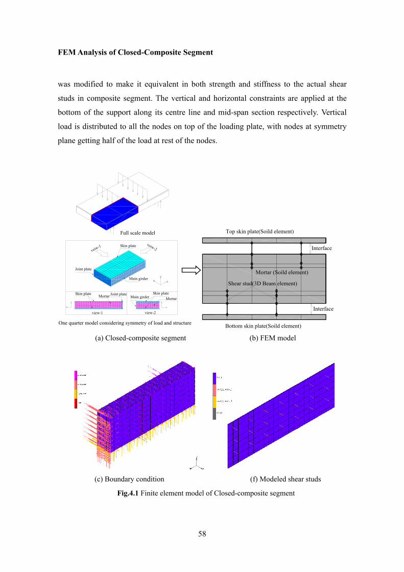
FEM Analysis of Closed-Composite Segment
58
was modified to make it equivalent in both strength and stiffness to the actual shear
studs in composite segment. The vertical and horizontal constraints are applied at the
bottom of the support along its centre line and mid-span section respectively. Vertical
load is distributed to all the nodes on top of the loading plate, with nodes at symmetry
plane getting half of the load at rest of the nodes.
Skin plateveiw-1
veiw-2
view-1 view-2
Skin plate
x
yz
y
x
y
z
Full scale model
Main girder
Joint plate
Main girder MortarJoint plateMortarSkin plate
One quarter model considering symmetry of load and structure Bottom skin plate(Soild element)
Shear stud(3D Beam element)
Top skin plate(Soild element)
Mortar (Soild element)
Interface
Interface
(a) Closed-composite segment (b) FEM model
(c) Boundary condition (f) Modeled shear studs
Fig.4.1 Finite element model of Closed-composite segment

The Mechanical Behavior and Design of Composite Segment for Shield Tunnel
59
4.2.2 Material Model
The material properties were obtained from elemental tests as presented in Chapter 2,
so material model used in finite element analysis are briefed in the following sections.
Incremental plastic flow theory is applied for the steel, shear connector and concrete
materials whereas nonlinear elasticity theory is applied for shear bond interaction. J2-
plasticity (von Mises) with associated flow rule is used for the steel material of the steel
tube and shear connector. In this case, the yield surface is independent of the hydrostatic
component of the stress vector as shown in Fig.4.2. The top skin plate buckling at the
maximum positive moment region was observed in some specimens, therefore, buckling
is assumed in the model. On the other hand, the concrete material is pressure dependent.
The general shape of failure surface for concrete material is illustrated in Fig.4.3.
MSC.Marc uses the Buyukozturk failure surface, a two-parameter model, for concrete
material (Buyukozturk 1975). This model is valid for the nonlinear response of concrete
under multi-axial compression.
Recent developments in the application of fracture mechanics to concrete in tension
enabled a fracture mechanics model to be used for the tensile portion of the concrete.
Concrete behavior in tension is assumed as linearly elastic. Concrete cracks, and softens
linearly until a strain of 0.005 where it completely loses its tensile load carrying capacity, when principal stress in tension reaches tensile strength tf ′ . Tensile softening
Failure surface
π plane
2σ
3σ
1σ
Hydrostatic axis
Yield surface
Failure surfaceπ plane2σ
3σ
1σ
Hydrostatic axis
Fig.4.2 Von Mises yield surface Fig.4.3 Concrete failure surface
in the principal stress space in the principal stress space
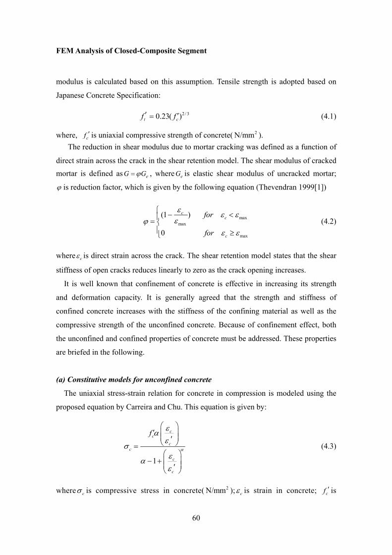
FEM Analysis of Closed-Composite Segment
60
modulus is calculated based on this assumption. Tensile strength is adopted based on
Japanese Concrete Specification:
2 / 30.23( )t cf f′ ′= (4.1)
where, cf ′ is uniaxial compressive strength of concrete( 2N/mm ). The reduction in shear modulus due to mortar cracking was defined as a function of
direct strain across the crack in the shear retention model. The shear modulus of cracked mortar is defined as eG Gϕ= , where eG is elastic shear modulus of uncracked mortar;
ϕ is reduction factor, which is given by the following equation (Thevendran 1999[1])
maxmax
max
(1 )
0
cc
c
for
for
ε ε εεϕ
ε ε
⎧ − <⎪= ⎨⎪ ≥⎩
(4.2)
where cε is direct strain across the crack. The shear retention model states that the shear
stiffness of open cracks reduces linearly to zero as the crack opening increases.
It is well known that confinement of concrete is effective in increasing its strength
and deformation capacity. It is generally agreed that the strength and stiffness of
confined concrete increases with the stiffness of the confining material as well as the
compressive strength of the unconfined concrete. Because of confinement effect, both
the unconfined and confined properties of concrete must be addressed. These properties
are briefed in the following.
(a) Constitutive models for unconfined concrete
The uniaxial stress-strain relation for concrete in compression is modeled using the
proposed equation by Carreira and Chu. This equation is given by:
1
cc
cc
c
c
f
α
εαε
σεαε
⎛ ⎞′ ⎜ ⎟⎜ ⎟′⎝ ⎠=
⎛ ⎞− + ⎜ ⎟⎜ ⎟′⎝ ⎠
(4.3)
where cσ is compressive stress in concrete( 2N/mm ); cε is strain in concrete; cf ′ is
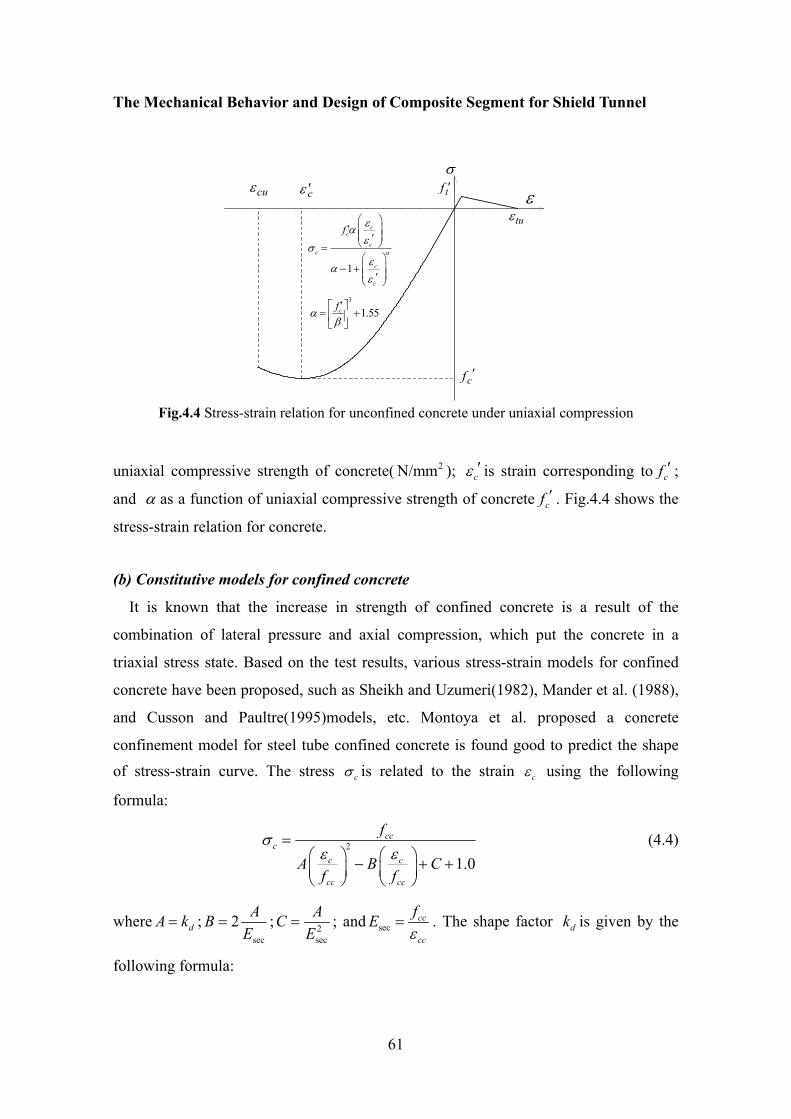
The Mechanical Behavior and Design of Composite Segment for Shield Tunnel
61
3
1.55cfαβ′⎡ ⎤
= +⎢ ⎥⎣ ⎦
1
cc
cc
c
c
f
α
εαε
σεαε
⎛ ⎞′ ⎜ ⎟⎜ ⎟′⎝ ⎠=
⎛ ⎞− + ⎜ ⎟⎜ ⎟′⎝ ⎠
cε ′
cuε
tuε
tf ′
cf ′
ε
σ
Fig.4.4 Stress-strain relation for unconfined concrete under uniaxial compression
uniaxial compressive strength of concrete( 2N/mm ); cε ′ is strain corresponding to cf ′ ;
and α as a function of uniaxial compressive strength of concrete cf ′ . Fig.4.4 shows the
stress-strain relation for concrete.
(b) Constitutive models for confined concrete
It is known that the increase in strength of confined concrete is a result of the
combination of lateral pressure and axial compression, which put the concrete in a
triaxial stress state. Based on the test results, various stress-strain models for confined
concrete have been proposed, such as Sheikh and Uzumeri(1982), Mander et al. (1988),
and Cusson and Paultre(1995)models, etc. Montoya et al. proposed a concrete
confinement model for steel tube confined concrete is found good to predict the shape of stress-strain curve. The stress cσ is related to the strain cε using the following
formula:
2
1.0
ccc
c c
cc cc
f
A B Cf f
σε ε
=⎛ ⎞ ⎛ ⎞− + +⎜ ⎟ ⎜ ⎟⎝ ⎠ ⎝ ⎠
(4.4)
where dA k= ;sec
2 ABE
= ; 2sec
ACE
= ; and seccc
cc
fEε
= . The shape factor dk is given by the
following formula:
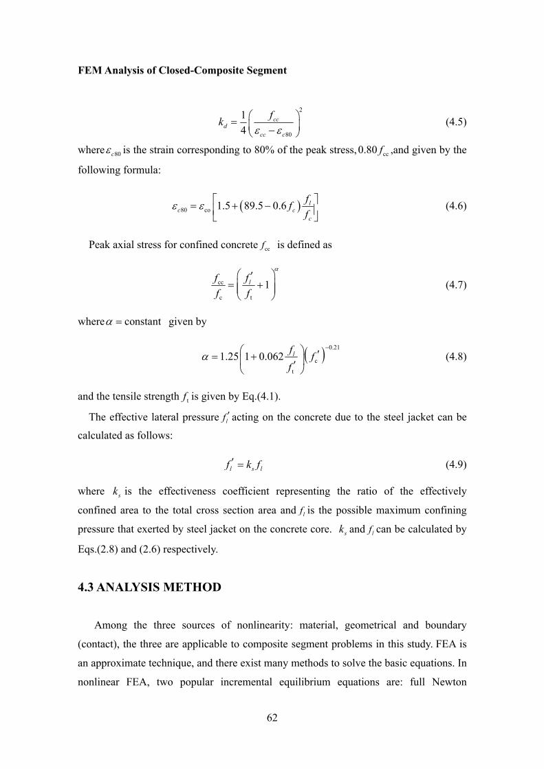
FEM Analysis of Closed-Composite Segment
62
2
80
14
ccd
cc c
fkε ε
⎛ ⎞= ⎜ ⎟−⎝ ⎠ (4.5)
where 80cε is the strain corresponding to 80% of the peak stress, cc0.80 f ,and given by the
following formula:
( )80 co 1.5 89.5 0.6 lc c
c
fff
ε ε ⎡ ⎤= + −⎢ ⎥⎣ ⎦ (4.6)
Peak axial stress for confined concrete ccf is defined as
cc
c t
1lf ff f
α⎛ ⎞′
= +⎜ ⎟⎜ ⎟⎝ ⎠
(4.7)
where constantα = given by
( ) 0.21
c
t
1.25 1 0.062 lf ff
α−⎛ ⎞ ′= +⎜ ⎟′⎝ ⎠
(4.8)
and the tensile strength tf is given by Eq.(4.1).
The effective lateral pressure lf ′acting on the concrete due to the steel jacket can be
calculated as follows:
l s lf k f′ = (4.9)
where sk is the effectiveness coefficient representing the ratio of the effectively
confined area to the total cross section area and lf is the possible maximum confining
pressure that exerted by steel jacket on the concrete core. sk and lf can be calculated by
Eqs.(2.8) and (2.6) respectively.
4.3 ANALYSIS METHOD
Among the three sources of nonlinearity: material, geometrical and boundary
(contact), the three are applicable to composite segment problems in this study. FEA is
an approximate technique, and there exist many methods to solve the basic equations. In
nonlinear FEA, two popular incremental equilibrium equations are: full Newton

The Mechanical Behavior and Design of Composite Segment for Shield Tunnel
63
-Raphson and modified Newton-Raphson. The full Newton-Raphson (N-R) method
assembles and solves the stiffness matrix for every iteration process. It has quadratic
convergence properties, which means in subsequent iterations the relative error
decreases quadratically. It gives good results for most nonlinear. Therefore, the full
Newton-Raphson (N-R) method is used in this study. The integration scheme used to
trace the equilibrium path is the arc-length method. The loading achieved by applying a
fixed displacement is distributed to all the nodes on top of the loading plate, and
convergence tolerance on displacement is defined as 0.1. Boundary (contact) and
geometrical nonlinearities are presented as the following sections.
4.3.1 Contact Analysis (Boundary Nonlinearity) Analysis is performed for slip condition to investigate the interface between
concrete and steel tube. A contact analysis possesses a provision for slip, and can be
used to simulate the slip between concrete and steel tube. Separate nodes are assigned
for concrete and steel tube at the same location. Frication is also considered in the
contact analysis for studying the interface between concrete and steel tube. In
MSC.Marc, the two available friction models are referred to in the documentation [2] as
the ‘Coulomb’ model and the ‘Stick-Slip’ model. The names are unfortunate since both
are approximate implementations of the theoretical Coulomb model. The following
sections briefly describe the implementation of these two friction models in MSC.Marc.
Full details can be found in [2]. Contact is a nonlinear boundary value problem. During
contact, mechanical loads and perhaps heat are transmitted across the area of contact. If
friction is present, shear forces are also transmitted. In MSC.Marc, areas of potential
contact do not need to be known prior to the analysis.
(a) Continuous Friction Model
The Coulomb friction law is expressed in the MSC.Marc documentation [1] as:
fr n tσ μσ≤ − ⋅ (4.10)
where nσ is the magnitude of the normal stress, frσ is the tangential (friction) stress
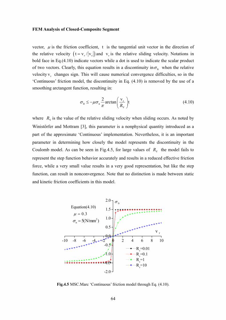
FEM Analysis of Closed-Composite Segment
64
vector, μ is the friction coefficient, t is the tangential unit vector in the direction of the relative velocity ( )r rt v / v= and rv is the relative sliding velocity. Notations in bold face in Eq.(4.10) indicate vectors while a dot is used to indicate the scalar product of two vectors. Clearly, this equation results in a discontinuity in frσ when the relative velocity rv changes sign. This will cause numerical convergence difficulties, so in the ‘Continuous’ friction model, the discontinuity in Eq. (4.10) is removed by the use of a smoothing arctangent function, resulting in:
rfr n
V
2 varctan tR
σ μσπ
⎛ ⎞≤ − ⎜ ⎟⎝ ⎠
(4.10)
where VR is the value of the relative sliding velocity when sliding occurs. As noted by
Winistőrfer and Mottram [3], this parameter is a nonphysical quantity introduced as a
part of the approximate ‘Continuous’ implementation. Nevertheless, it is an important
parameter in determining how closely the model represents the discontinuity in the Coulomb model. As can be seen in Fig.4.5, for large values of VR the model fails to
represent the step function behavior accurately and results in a reduced effective friction
force, while a very small value results in a very good representation, but like the step
function, can result in nonconvergence. Note that no distinction is made between static
and kinetic friction coefficients in this model.
-10 -8 -6 -4 -2 0 2 4 6 8 10
-2.0
-1.5
-1.0
-0.5
0.0
0.5
1.0
1.5
2.0Equation(4.10)
2n 5(N/mm )σ =
0.3μ =
rv
frσ
Rv=0.01Rv=0.1Rv=1Rv=10
Fig.4.5 MSC.Marc ‘Continuous’ friction model through Eq. (4.10).
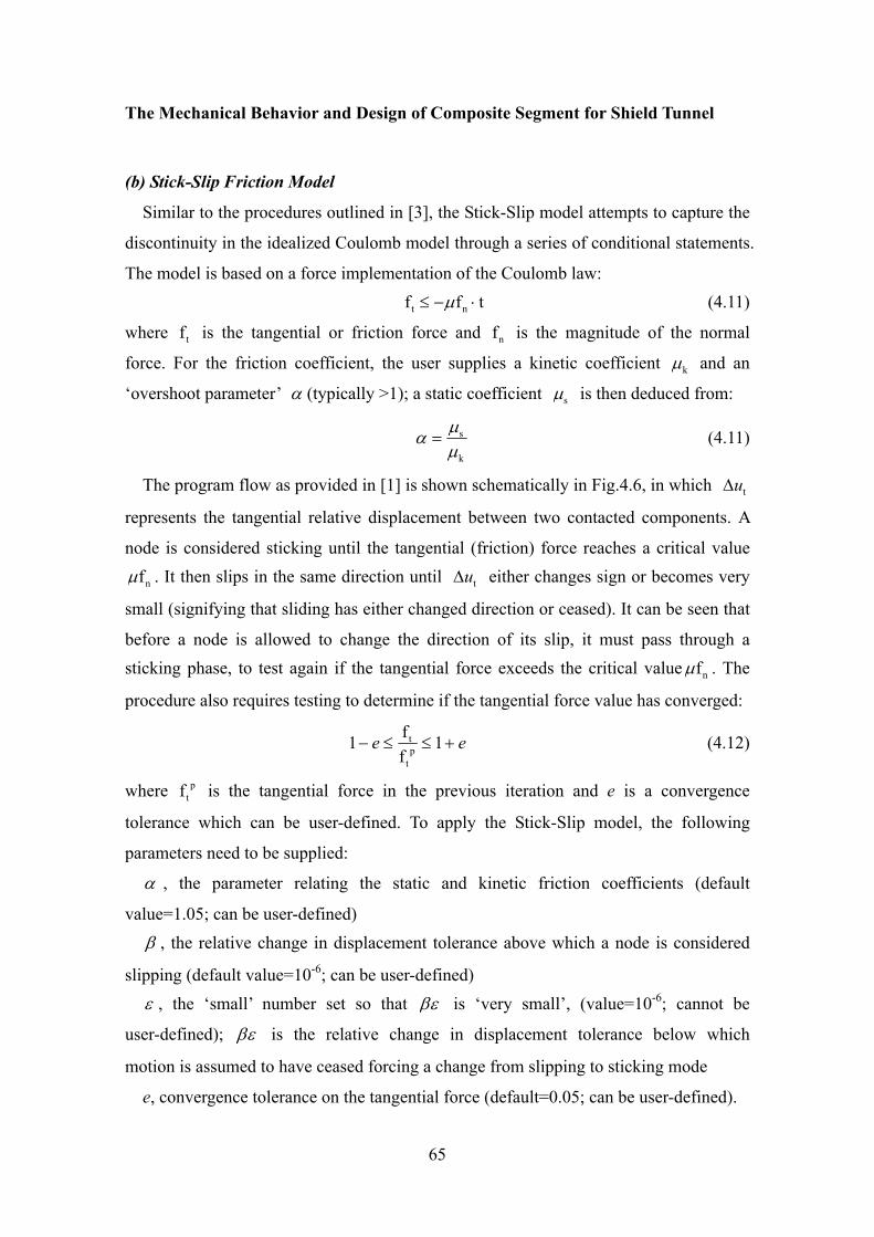
The Mechanical Behavior and Design of Composite Segment for Shield Tunnel
65
(b) Stick-Slip Friction Model
Similar to the procedures outlined in [3], the Stick-Slip model attempts to capture the
discontinuity in the idealized Coulomb model through a series of conditional statements.
The model is based on a force implementation of the Coulomb law:
t nf f tμ≤ − ⋅ (4.11)
where tf is the tangential or friction force and nf is the magnitude of the normal
force. For the friction coefficient, the user supplies a kinetic coefficient kμ and an
‘overshoot parameter’ α (typically >1); a static coefficient sμ is then deduced from:
s
k
μαμ
= (4.11)
The program flow as provided in [1] is shown schematically in Fig.4.6, in which tuΔ
represents the tangential relative displacement between two contacted components. A
node is considered sticking until the tangential (friction) force reaches a critical value
nfμ . It then slips in the same direction until tuΔ either changes sign or becomes very
small (signifying that sliding has either changed direction or ceased). It can be seen that
before a node is allowed to change the direction of its slip, it must pass through a sticking phase, to test again if the tangential force exceeds the critical value nfμ . The
procedure also requires testing to determine if the tangential force value has converged:
tp
t
f1 1f
e e− ≤ ≤ + (4.12)
where ptf is the tangential force in the previous iteration and e is a convergence
tolerance which can be user-defined. To apply the Stick-Slip model, the following
parameters need to be supplied:
α , the parameter relating the static and kinetic friction coefficients (default
value=1.05; can be user-defined) β , the relative change in displacement tolerance above which a node is considered
slipping (default value=10-6; can be user-defined) ε , the ‘small’ number set so that βε is ‘very small’, (value=10-6; cannot be
user-defined); βε is the relative change in displacement tolerance below which
motion is assumed to have ceased forcing a change from slipping to sticking mode
e, convergence tolerance on the tangential force (default=0.05; can be user-defined).
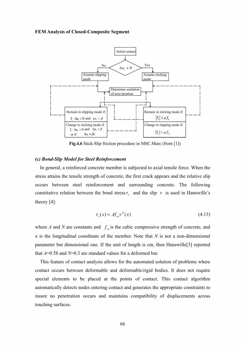
FEM Analysis of Closed-Composite Segment
66
t s nf fμ≤
t s nf fμ>tu βεΔ ≈or if
tu βΔ >andt tf 0u⋅Δ >
tu βΔ >andt tf 0u⋅Δ <
t 0uΔ ≈
Remain in sticking mode if:
Change to slipping mode if:
Remain in slipping mode if:
Change to sticking mode if:
No Yes
Determine soulutionof next iteration
Assume sticking mode
Assume slipping mode
Initial contact
Fig.4.6 Stick-Slip friction procedure in MSC.Marc (from [1])
(c) Bond-Slip Model for Steel Reinforcement
In general, a reinforced concrete member is subjected to axial tensile force. When the
stress attains the tensile strength of concrete, the first crack appears and the relative slip
occurs between steel reinforcement and surrounding concrete. The following constitutive relation between the bond stress vτ and the slip v is used in Hanswille’s
theory [4]:
( ) ( )Nv cux Af v xτ = (4.13)
where A and N are constants and cuf is the cubic compressive strength of concrete, and
x is the longitudinal coordinate of the member. Note that N is not a non-dimensional
parameter but dimensional one. If the unit of length is cm, then Hanswille[3] reported
that A=0.58 and N=0.3 are standard values for a deformed bar.
This feature of contact analysis allows for the automated solution of problems where
contact occurs between deformable and deformable/rigid bodies. It does not require
special elements to be placed at the points of contact. This contact algorithm
automatically detects nodes entering contact and generates the appropriate constraints to
insure no penetration occurs and maintains compatibility of displacements across
touching surfaces.
The Mechanical Behavior and Design of Composite Segment for Shield Tunnel
67
4.3.2 Buckling Analysis (Geometrical Nonlinearity) In MSC.Marc[1], Buckling analysis allows the user to determine at what load the
structure will collapse. It can detect the buckling of a structure when the structure’s
stiffness matrix approaches a singular value. It can extract the eigenvalue in a linear
analysis to obtain the linear buckling load. It can also perform eigenvalue analysis for
buckling load in a nonlinear problem based on the incremental stiffness matrices.
The buckling option estimates the maximum load that can be applied to a
geometrically nonlinear structure before instability sets in. To activate the buckling
option in the program, use the parameter BUCKLE. If a nonlinear buckling analysis is
performed, also use the parameter LARGE DISP.
Use the history definition option BUCKLE to input control tolerances for buckling
load estimation (eigenvalue extraction by a power sweep or Lanczos method). It can
estimate the buckling load after every load increment. The BUCKLE INCREMENT
option can be used if a collapse load calculation is required at multiple increments.
The linear buckling load analysis is correct when take a very small load step in
increment zero, or make sure the solution has converged before buckling load analysis
(if multiple increments are taken). Linear buckling (after increment zero) can be done
without using the LARGE DISP parameter, in which case the restriction on the load step
size no longer applies. This value should be used with caution, as it is not conservative
in predicting the actual collapse of structures.
In a buckling problem that involves material nonlinearity (for example, plasticity),
the nonlinear problem must be solved incrementally. During the analysis, a failure to
converge in the iteration process or nonpositive definite stiffness signals the plastic
collapse.
For extremely nonlinear problems, the BUCKLE option cannot produce accurate
results. In that case, the history definition option AUTO INCREMENT allows automatic
load stepping in a quasi-static fashion for both geometric large displacement and
material (elastic-plastic) nonlinear problems. The option can handle elastic-plastic
snap-through phenomena. Therefore, the post-buckling behavior of structures can be
analyzed. Full details can be found in [1].
FEM Analysis of Closed-Composite Segment
68
The buckling option solves the following eigenvalue problem by the inverse power
sweep method:
( ), , 0GK K u uλ σ φ+ Δ Δ Δ =⎡ ⎤⎣ ⎦ (4.14)
where GKΔ is assumed to be a linear function of the load increment to PΔ cause
buckling.
The geometric stiffness used for the buckling load calculation is based on the stress
and displacement state change at the start of the last increment. However, the stress and
strain states are not updated during the buckling analysis. The buckling load is therefore
estimated by:
(beginning)P Pλ+ Δ (4.15)
where for increments greater than 1, (beginning)P is the load applied at the beginning
of the increment prior to the buckling analyses, and λ is the value obtained by the
power sweep or Lanczos method.
The control tolerances for the inverse power sweep method are the maximum number
of iterations in the power sweep and the convergence tolerance. The power sweep
terminates when the difference between the eigenvalues in two consecutive sweeps
divided by the eigenvalue is less than the tolerance. The Lanczos method concludes
when the normalized difference between all eigenvalues satisfies the tolerance. The
maximum number of iterations and the tolerance are specified through the BUCKLE
history definition option.
4.4 RESULTS OF ANALYSIS AND DISCUSSION
All composite segment specimens were analyzed using 3D finite element analysis of
MSC.Marc software package. Parameters of Closed-segment specimens are described in
Chapter 3.2.1. Initially, a Closed-composite segment specimen was analyzed with an
assumption of perfect bond between steel tube and concrete infill. It can be seen that the
stiffness of analysis result is larger than that of the experimental result shown in Fig.4.7.
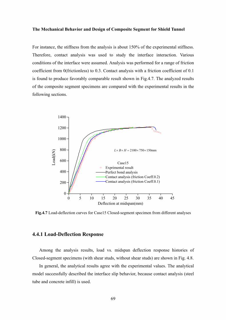
The Mechanical Behavior and Design of Composite Segment for Shield Tunnel
69
For instance, the stiffness from the analysis is about 150% of the experimental stiffness.
Therefore, contact analysis was used to study the interface interaction. Various
conditions of the interface were assumed. Analysis was performed for a range of friction
coefficient from 0(frictionless) to 0.3. Contact analysis with a friction coefficient of 0.1
is found to produce favorably comparable result shown in Fig.4.7. The analyzed results
of the composite segment specimens are compared with the experimental results in the
following sections.
0 5 10 15 20 25 30 35 40 450
200
400
600
800
1000
1200
1400
2100 750 150mmL B H× × = × ×
Load
(kN
)
Deflection at midspan(mm)
Case15Exprimental result Perfect bond analysis Contact analysis (friction Coeff.0.2)Contact analysis (friction Coeff.0.1)
Fig.4.7 Load-deflection curves for Case15 Closed-segment specimen from different analyses
4.4.1 Load-Deflection Response
Among the analysis results, load vs. midspan deflection response histories of
Closed-segment specimens (with shear studs, without shear studs) are shown in Fig. 4.8.
In general, the analytical results agree with the experimental values. The analytical
model successfully described the interface slip behavior, because contact analysis (steel
tube and concrete infill) is used.
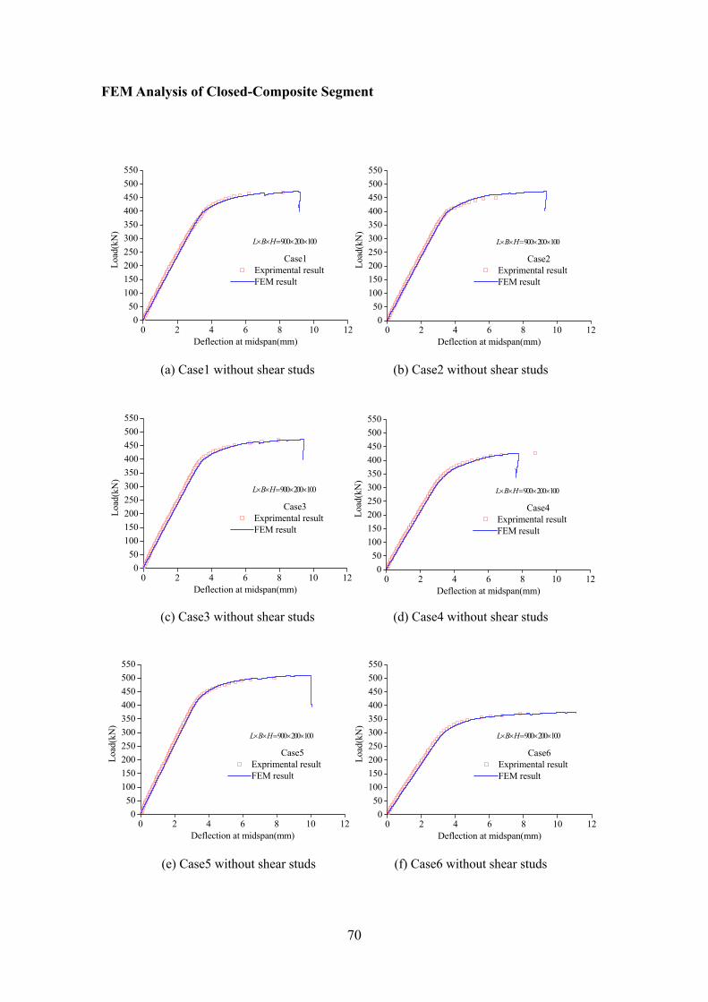
FEM Analysis of Closed-Composite Segment
70
0 2 4 6 8 10 120
50100150200250300350400450500550
900 200 100L B H× × = × ×
Load
(kN
)
Deflection at midspan(mm)
Case1Exprimental result FEM result
0 2 4 6 8 10 120
50100150200250300350400450500550
900 200 100L B H× × = × ×
Load
(kN
)
Deflection at midspan(mm)
Case2Exprimental result FEM result
(a) Case1 without shear studs (b) Case2 without shear studs
0 2 4 6 8 10 120
50100150200250300350400450500550
900 200 100L B H× × = × ×
Load
(kN
)
Deflection at midspan(mm)
Case3Exprimental result FEM result
0 2 4 6 8 10 120
50100150200250300350400450500550
900 200 100L B H× × = × ×
Load
(kN
)
Deflection at midspan(mm)
Case4Exprimental result FEM result
(c) Case3 without shear studs (d) Case4 without shear studs
0 2 4 6 8 10 120
50100150200250300350400450500550
900 200 100L B H× × = × ×
Load
(kN
)
Deflection at midspan(mm)
Case5Exprimental result FEM result
0 2 4 6 8 10 120
50100150200250300350400450500550
900 200 100L B H× × = × ×
Load
(kN
)
Deflection at midspan(mm)
Case6Exprimental result FEM result
(e) Case5 without shear studs (f) Case6 without shear studs

The Mechanical Behavior and Design of Composite Segment for Shield Tunnel
71
0 2 4 6 8 10 120
50100150200250300350400450500550600
900 200 100L B H× × = × ×
Load
(kN
)
Deflection at midspan(mm)
Case7Exprimental result FEM result
0 2 4 6 8 10 120
50
100
150
200
250
300
350
400
450
900 200 100L B H× × = × ×
Load
(kN
)
Deflection at midspan(mm)
Case8Exprimental result FEM result
(g) Case7 without shear studs (h) Case8 without shear studs
0 5 10 15 20 25 300
50
100
150
200
250
300
350
400
450
900 300 100L B H× × = × ×
Load
(kN
)
Deflection at midspan(mm)
Case9Exprimental result FEM result
0 3 6 9 12 150
100
200
300
400
500
600
700
800
900 500 100mmL B H× × = × ×
Load
(kN
)
Deflection at midspan(mm)
Case10Exprimental result FEM result
(i) Case9 without shear studs (j) Case10 without shear studs
0 5 10 15 20 250
50
100
150
200
250
300
350
400
450
900 200 100L B H× × = × ×
Load
(kN
)
Deflection at midspan(mm)
Case11Exprimental result FEM result
0 5 10 15 20 25 300
50
100
150
200
250
300
350
400
450
900 300 100L B H× × = × ×
Load
(kN
)
Deflection at midspan(mm)
Case12Exprimental result FEM result
(k) Case11 with shear studs (l) Case12 with shear studs
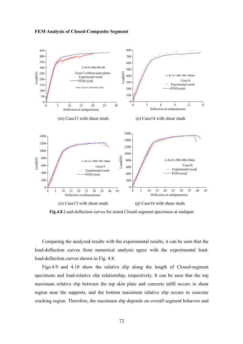
FEM Analysis of Closed-Composite Segment
72
0 5 10 15 20 25 300
50
100
150
200
250
300
350
400
450
Note: Case13 with shear studs
900 300 100L B H× × = × ×
Load
(kN
)
Deflection at midspan(mm)
Case13 without joint platesExprimental result FEM result
0 3 6 9 12 15
0
100
200
300
400
500
600
700
800
900 500 100mmL B H× × = × ×
Load
(kN
)
Deflection at midspan(mm)
Case14Exprimental result FEM result
(m) Case13 with shear studs (n) Case14 with shear studs
0 5 10 15 20 25 30 35 40 450
200
400
600
800
1000
1200
1400
2100 750 150mmL B H× × = × ×
Load
(kN
)
Deflection at midspan(mm)
Case15Exprimental result FEM result
0 5 10 15 20 25 30 35 40 450
200
400
600
800
1000
1200
1400
1600
2100 1000 150mmL B H× × = × ×
Load
(kN
)
Deflection at midspan(mm)
Case16Exprimental result FEM result
(o) Case15 with shear studs (p) Case16 with shear studs
Fig.4.8 Load-deflection curves for tested Closed-segment specimens at midspan
Comparing the analyzed results with the experimental results, it can be seen that the
load-deflection curves from numerical analysis agree with the experimental load-
load-deflection curves shown in Fig. 4.8.
Figs.4.9 and 4.10 show the relative slip along the length of Closed-segment
specimens and load-relative slip relationship, respectively. It can be seen that the top
maximum relative slip between the top skin plate and concrete infill occurs in shear
region near the supports, and the bottom maximum relative slip occurs in concrete
cracking region. Therefore, the maximum slip depends on overall segment behavior and
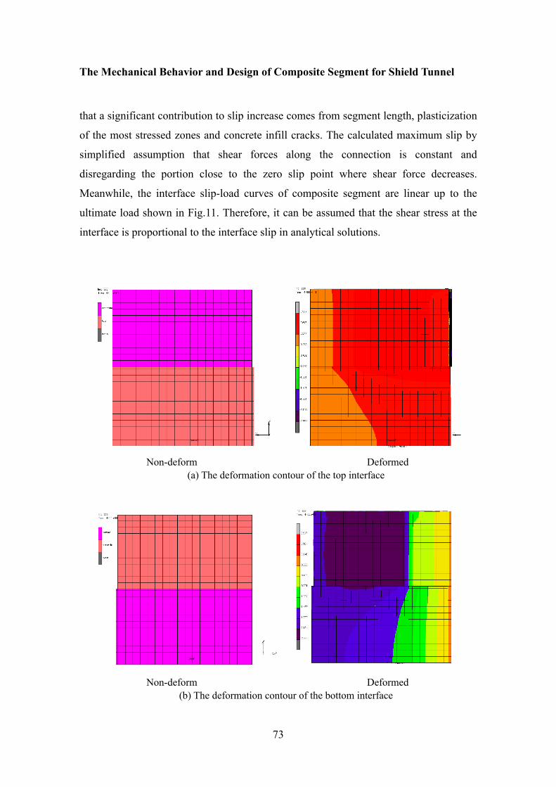
The Mechanical Behavior and Design of Composite Segment for Shield Tunnel
73
that a significant contribution to slip increase comes from segment length, plasticization
of the most stressed zones and concrete infill cracks. The calculated maximum slip by
simplified assumption that shear forces along the connection is constant and
disregarding the portion close to the zero slip point where shear force decreases.
Meanwhile, the interface slip-load curves of composite segment are linear up to the
ultimate load shown in Fig.11. Therefore, it can be assumed that the shear stress at the
interface is proportional to the interface slip in analytical solutions.
Non-deform Deformed
(a) The deformation contour of the top interface
Non-deform Deformed (b) The deformation contour of the bottom interface

FEM Analysis of Closed-Composite Segment
74
0 50 100 150 200 250 300 350 400 4500.0
0.4
0.8
1.2
1.6
2.0
Case10 without shear stud relative slip between top skin plate and concrete infill relative slip between bottom skin plate and concrete infill
900 500 100mmL B H× × = × ×
Hor
izon
tal r
elat
ive
slip
(mm
)
Half length of closed-composite segment(mm) Fig.4.9 Relative slip distribution for Closed-segment specimens without shear studs of Case10
Non-deform Deformed
(a) The deformation contour of the top interface
Non-deform Deformed
(b) The deformation contour of the bottom interface
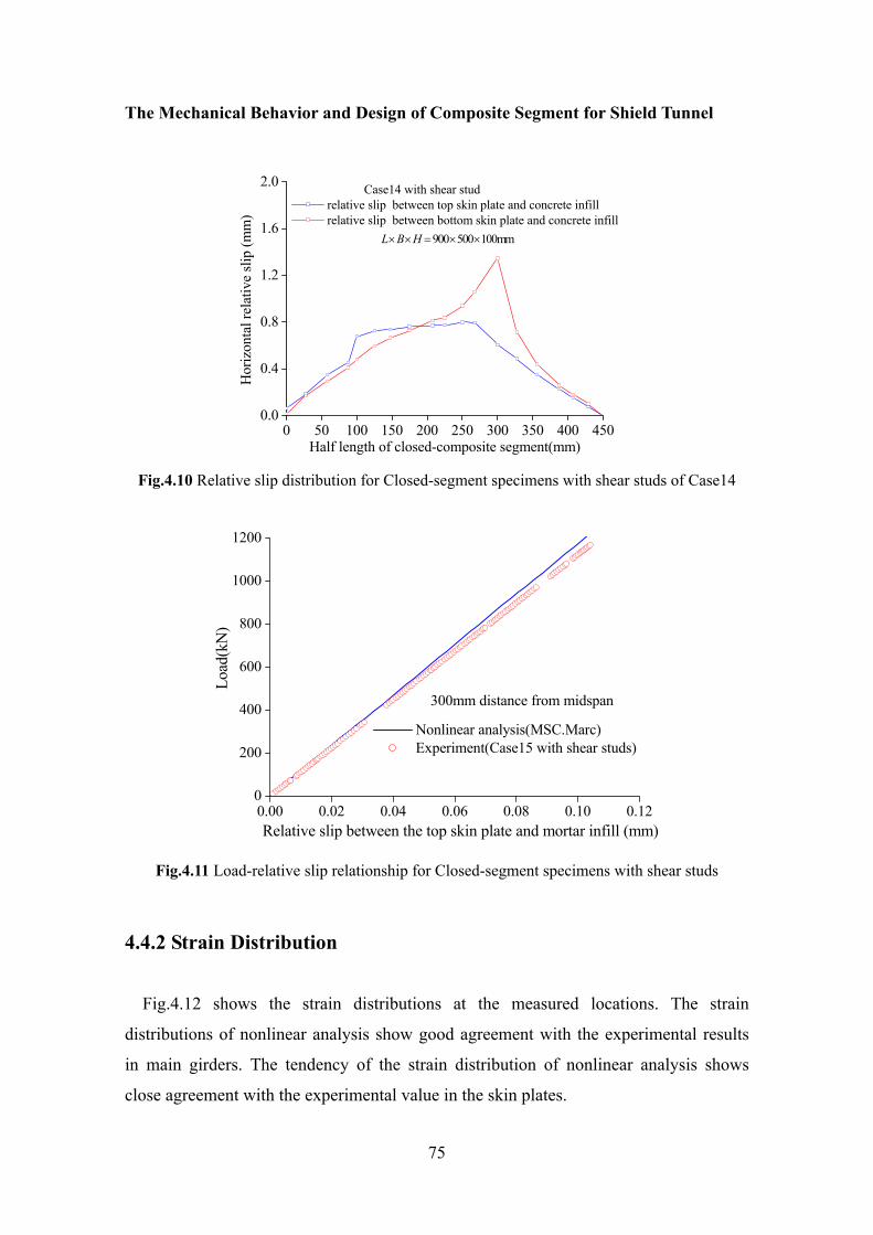
The Mechanical Behavior and Design of Composite Segment for Shield Tunnel
75
0 50 100 150 200 250 300 350 400 4500.0
0.4
0.8
1.2
1.6
2.0 Case14 with shear stud relative slip between top skin plate and concrete infill relative slip between bottom skin plate and concrete infill
900 500 100mmL B H× × = × ×H
oriz
onta
l rel
ativ
e sli
p (m
m)
Half length of closed-composite segment(mm)
Fig.4.10 Relative slip distribution for Closed-segment specimens with shear studs of Case14
0.00 0.02 0.04 0.06 0.08 0.10 0.120
200
400
600
800
1000
1200
300mm distance from midspan
Load
(kN
)
Relative slip between the top skin plate and mortar infill (mm)
Nonlinear analysis(MSC.Marc) Experiment(Case15 with shear studs)
Fig.4.11 Load-relative slip relationship for Closed-segment specimens with shear studs
4.4.2 Strain Distribution
Fig.4.12 shows the strain distributions at the measured locations. The strain
distributions of nonlinear analysis show good agreement with the experimental results
in main girders. The tendency of the strain distribution of nonlinear analysis shows
close agreement with the experimental value in the skin plates.
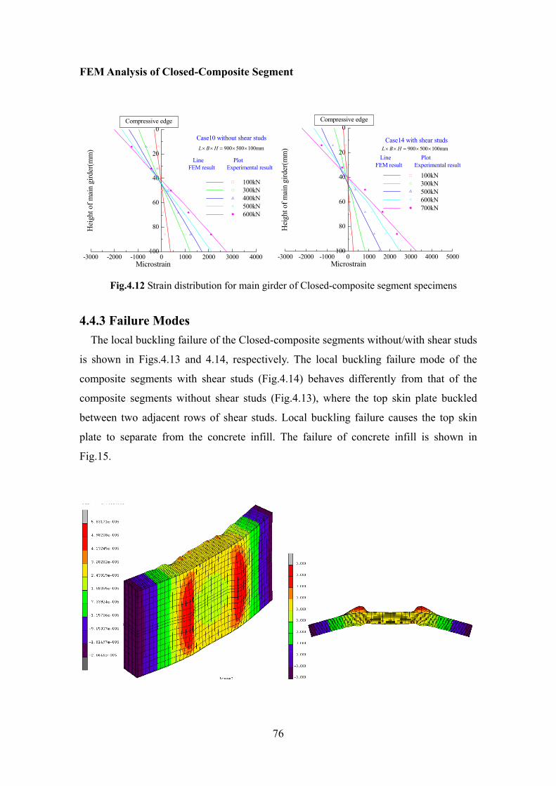
FEM Analysis of Closed-Composite Segment
76
-3000 -2000 -1000 0 1000 2000 3000 4000100
80
60
40
20
0
Line PlotFEM result Experimental result
900 500 100mmL B H× × = × ×
100kN 300kN 400kN 500kN 600kN
Case10 without shear studs
Hei
ght o
f mai
n gi
rder
(mm
)
Compressive edge
Microstrain
-3000 -2000 -1000 0 1000 2000 3000 4000 5000100
80
60
40
20
0
Line PlotFEM result Experimental result
100kN 300kN 500kN 600kN 700kN
900 500 100mmL B H× × = × ×Case14 with shear studs
Hei
ght o
f mai
n gi
rder
(mm
)
Compressive edge
Microstrain
Fig.4.12 Strain distribution for main girder of Closed-composite segment specimens
4.4.3 Failure Modes
The local buckling failure of the Closed-composite segments without/with shear studs
is shown in Figs.4.13 and 4.14, respectively. The local buckling failure mode of the
composite segments with shear studs (Fig.4.14) behaves differently from that of the
composite segments without shear studs (Fig.4.13), where the top skin plate buckled
between two adjacent rows of shear studs. Local buckling failure causes the top skin
plate to separate from the concrete infill. The failure of concrete infill is shown in
Fig.15.

The Mechanical Behavior and Design of Composite Segment for Shield Tunnel
77
Fig.4.13 Local buckling of Closed-composite segment specimens without shear studs
Fig.4.14 Local buckling failure of Closed-composite segment specimens with shear studs
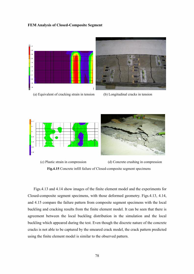
FEM Analysis of Closed-Composite Segment
78
(a) Equivalent of cracking strain in tension (b) Longitudinal cracks in tension
(c) Plastic strain in compression (d) Concrete crushing in compression
Fig.4.15 Concrete infill failure of Closed-composite segment specimens
Figs.4.13 and 4.14 show images of the finite element model and the experiments for
Closed-composite segment specimens, with those deformed geometry. Figs.4.13, 4.14,
and 4.15 compare the failure pattern from composite segment specimens with the local
buckling and cracking results from the finite element model. It can be seen that there is
agreement between the local buckling distribution in the simulation and the local
buckling which appeared during the test. Even though the discrete nature of the concrete
cracks is not able to be captured by the smeared crack model, the crack pattern predicted
using the finite element model is similar to the observed pattern.

The Mechanical Behavior and Design of Composite Segment for Shield Tunnel
79
4.4.4 Contact Status
Contact status, contact force were carefully analyzed throughout the incremental
solution and the model incorporating a non-positive definite solution seemed to be of
satisfactory quality because no anomalies existed in the stresses or strains and contact
penetration was not evident. Fig.4.16 shows the images of contact status and contact
force of Closed-composite segment specimens.
(a) 600kN contact status (without shear studs)
(b) 600kN contact status (with shear studs)
Fig.4.16 Contact status of Closed-composite segment specimens
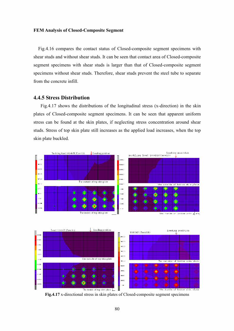
FEM Analysis of Closed-Composite Segment
80
Fig.4.16 compares the contact status of Closed-composite segment specimens with
shear studs and without shear studs. It can be seen that contact area of Closed-composite
segment specimens with shear studs is larger than that of Closed-composite segment
specimens without shear studs. Therefore, shear studs prevent the steel tube to separate
from the concrete infill.
4.4.5 Stress Distribution
Fig.4.17 shows the distributions of the longitudinal stress (x-direction) in the skin
plates of Closed-composite segment specimens. It can be seen that apparent uniform
stress can be found at the skin plates, if neglecting stress concentration around shear
studs. Stress of top skin plate still increases as the applied load increases, when the top
skin plate buckled.
Fig.4.17 x-directional stress in skin plates of Closed-composite segment specimens

The Mechanical Behavior and Design of Composite Segment for Shield Tunnel
81
It can be seen from Fig.4.17 that the local buckling of the skin plate in compression
should be adopted in analysis and design of composite segment, according to different
degree of shear connection. The skin plate in tension can be assumed as the member of
full effective cross-section.
4.5 DISCUSSION OF CONTACT ANALYSIS
All Closed-composite segment specimens were analyzed with an assumption of
perfect bond between concrete infill and steel tube. Closed-composite segment
specimens were found too stiff from the analysis as compared to the experimental
results shown in Fig.4.18.Later, contact analysis was performed to study the interface
interaction, and Coulomb friction model was used in this study. Various conditions of
the interface were assumed. Analysis was performed for a range of friction coefficient
from 0 (frictionless) to 0.3. Contact analysis with a friction coefficient of 0.1, and the relative sliding velocity ( VR ) of default value 0.1 are found to produce favorably
comparable result shown in Figs.4.8 and 4.18.
0 5 10 15 20 25 30 35 40 450
200
400
600
800
1000
1200
1400
2100 750 150mmL B H× × = × ×
Load
(kN
)
Deflection at midspan(mm)
Case15Exprimental result Contact analysis (friction Coeff.0.2)Contact analysis (friction Coeff.0.1)Contact analysis (frictionless)
Fig.4.18 Effect of friction on the stiffness of Closed-composite segment specimens
FEM Analysis of Closed-Composite Segment
82
4.6. SUMMARY
The proposed finite element model using MSC.Marc have been examined for their
ability to simulate the mechanical behavior of Closed-composite segments. The main
conclusions are obtained as follows:
(1) Contact analysis was found to be able to simulate the slip at the interface between
steel tube and concrete infill. For the composite segments with no axial load,
frictionless condition could simulate the load-deflection curves from the
experimental results. For the composite segments, a friction coefficient of 0.1
produced convincing results.
(2) Discrete shear studs modeled using 3D beam elements is able to simulate the
mechanical behavior of shear connectors.
(3) The effective width of the skin plate in compression should be adopted in analysis
and design of composite segment, according to different degree of shear connection.
The skin plate in tension can be assumed as the member of full effective
cross-section.
4.7. REFERENCES
1) Thevendran, V., et al,1999. Nonlinear analysis of steel-concrete composite beams
curved in plan. Finite Elem. Anal. Design, 32(3), 125-139.
2) MSC.Marc Documentation, 2005. Volume A Theory and User Information. MSC
Software.
3) Winistőrfer, A. and Mottram, J.T, 2001. Finite Element Analysis of Non-Laminated
Composite Pin-Loaded Straps for Civil Engineering, Journal of Composites Materials,
35(7):577–601.
4) Hanswille, G,1986. Zur Rißbreitenbeschränkung bei Verbundträgern, Technisch-
Weissenschaftliche Mitteilungen, Institut für Konstruktiven Ingenieurbau
Ruhr-Universität Bochum, Mittelilung Nr. 86-1.

The Mechanical Behavior and Design of Composite Segment for Shield Tunnel
83
Chapter 5. A Mechanical Model of Closed-Composite Segment
5.1 INTRODUCTION
In general, many underground structures are designed by the allowable stress design
method. In this method various indeterminate factors such as variations in material
properties, acting loads, precision of estimated design loads, analysis model and
structural calculation method etc., are simply assumed based on factors of safety.
Shield tunnel linings (hereinafter called as segment rings) consist of segments and
many connecting joints, and show complicated mechanical behavior under combined
loads. Meanwhile, it is difficult to precisely define the loads acting on segment rings due
to variation in construction conditions. Therefore, the allowable stress design method as
a simplified solution is still used in the design of segments for shield tunnel.
However, it is possible to predict the variations in acting loads and material properties
etc., because of the high technical developments of FEA and measuring method for the
last few years. Therefore, the allowable stress design method is not rational in economy,
because it is not able to directly evaluate the variations in material strength, member size,
and loads etc. On the contrary, the limit state design is able to evaluate the variations in
material strength, member size, and loads etc using factors of safety based on the
theories of probability, statistics, and reliability.
The limit state design requires the structure to satisfy two principal criteria: the
ultimate limit state (ULS) and the serviceability limit state (SLS). A limit state is a set of
performance criteria (e.g. vibration levels, deflection, strength, stability, buckling,
twisting, collapse) that must be met when the structure is subject to loads.
To satisfy the ultimate limit state, the structure must not collapse when subjected to
the peak design load for which it was designed. A structure is deemed to satisfy the
ultimate limit state criteria if all factored bending, shear, and tensile or compressive
stresses are below the factored resistance calculated for the section under consideration.
The limit state criteria can also be set in terms of stress rather than load. Thus the
structural element being analyzed (e.g. a beam or a column or other load carrying
element, such as walls) is shown to be safe when the factored loads are less than their
A Mechanical Model of Closed-Composite Segment
84
factored resistance.
To satisfy the serviceability limit state criteria, a structure must remain functional for
its intended use subject to service loads, and as such the structure must not cause
occupant discomfort under design life.
It is true problem that the limit state design is not currently used in the segment design
for shield tunnel. Therefore, one of the purposes of developing a mechanical model for
composite segment is to provide tools suitable for limit state design. The paper does not
address safety coefficients as its purpose is to underscore the phenomena involved in the
issue rather than measuring structural safety.
The proposed mechanical model analyzes the nonlinear behavior of a composite
segment with discrete partial shear connection under combined loads. This model is
based on the two fields mixed force-displacement equation with nonlinear constitutive
relationships for the components. The tension stiffening effect is taken into account by
using the relationship proposed in the CEB-FIB Model Code 90 [1]. The model
considers the concept of partial interaction allowing for the occurrence of slip at the
interface between steel tube and concrete infill, and local buckling of steel plate in
compression.
5.2 STRUCTURAL MODELING
The main ingredients of the proposed formulas consists of (a) fiber element formulas
for the composite segment; (b) nonlinear constitutive relationships for the component
materials; (c) model for steel embedded in concrete.
5.2.1 Basic Assumptions Following the analytical method for the composite segment, it is assumed that:
(1) Throughout the depth of the cross-section, the strain distribution is linear, but a
discontinuity exists at the interface between steel tube and concrete infill due to
slip;
(2) No uplift or vertical separation occurs between steel tube and concrete infill;
therefore two parts of the composite section have the same rotation and the same
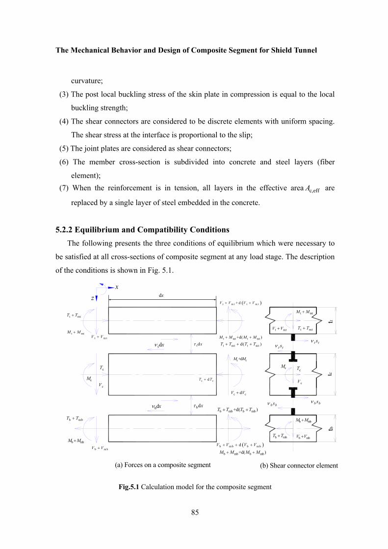
The Mechanical Behavior and Design of Composite Segment for Shield Tunnel
85
curvature;
(3) The post local buckling stress of the skin plate in compression is equal to the local
buckling strength;
(4) The shear connectors are considered to be discrete elements with uniform spacing.
The shear stress at the interface is proportional to the slip;
(5) The joint plates are considered as shear connectors;
(6) The member cross-section is subdivided into concrete and steel layers (fiber
element); (7) When the reinforcement is in tension, all layers in the effective area c,effA are
replaced by a single layer of steel embedded in the concrete.
5.2.2 Equilibrium and Compatibility Conditions The following presents the three conditions of equilibrium which were necessary to
be satisfied at all cross-sections of composite segment at any load stage. The description
of the conditions is shown in Fig. 5.1.
(b) Shear connector element(a) Forces on a composite segment
tc
b bsν b bsν
t tsνt tsν
zx
cV
cTcM
tttb
bdxν
tdxν
b mbV V+
b mbM M+
b mbT T+
t mtV V+ t mtT T+
t mtM M+
bdxτ
tdxτ
( )b m b b m bdV V V V+ + +
c cdV V+
t mt t mtd( )T T T T+ + +t mt t mt+d( )M M M M+ +
c c+dM M
c cdT T+
b mb b mb+d( )M M M M+ +
b mb b mb+d( )T T T T+ +
( )t m t t m t+ dV V V V+ +
b m bV V+
cV
t m tV V+
b mbM M+
b mbT T+
cT
cM
t mtT T+
t mtM M+
dx
Fig.5.1 Calculation model for the composite segment
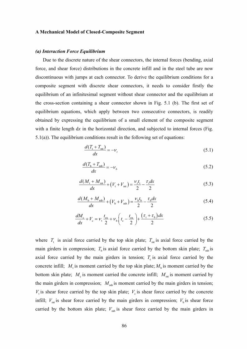
A Mechanical Model of Closed-Composite Segment
86
(a) Interaction Force Equilibrium
Due to the discrete nature of the shear connectors, the internal forces (bending, axial
force, and shear force) distributions in the concrete infill and in the steel tube are now
discontinuous with jumps at each connector. To derive the equilibrium conditions for a
composite segment with discrete shear connectors, it needs to consider firstly the
equilibrium of an infinitesimal segment without shear connector and the equilibrium at
the cross-section containing a shear connector shown in Fig. 5.1 (b). The first set of
equilibrium equations, which apply between two consecutive connectors, is readily
obtained by expressing the equilibrium of a small element of the composite segment
with a finite length dx in the horizontal direction, and subjected to internal forces (Fig.
5.1(a)). The equilibrium conditions result in the following set of equations:
t mt( )t
d T Tdx
ν+= − (5.1)
b mb( )b
d T Tdx
ν+= − (5.2)
( )t mt t t tt mt
( )2 2
d M M t dxV Vdx
ν τ++ + = − (5.3)
( )b mb b b bb mb
( )2 2
d M M t dxV Vdx
ν τ++ + = − (5.4)
( )t bc cu cuc t b c2 2 2
dxdM t tV tdx
τ τν ν
+⎛ ⎞+ = + − +⎜ ⎟⎝ ⎠
(5.5)
where tT is axial force carried by the top skin plate; mtT is axial force carried by the
main girders in compression; bT is axial force carried by the bottom skin plate; mbT is
axial force carried by the main girders in tension; cT is axial force carried by the
concrete infill; tM is moment carried by the top skin plate; bM is moment carried by the
bottom skin plate; cM is moment carried the concrete infill; mtM is moment carried by
the main girders in compression; mbM is moment carried by the main girders in tension;
tV is shear force carried by the top skin plate; cV is shear force carried by the concrete
infill; mtV is shear force carried by the main girders in compression; bV is shear force
carried by the bottom skin plate; mbV is shear force carried by the main girders in
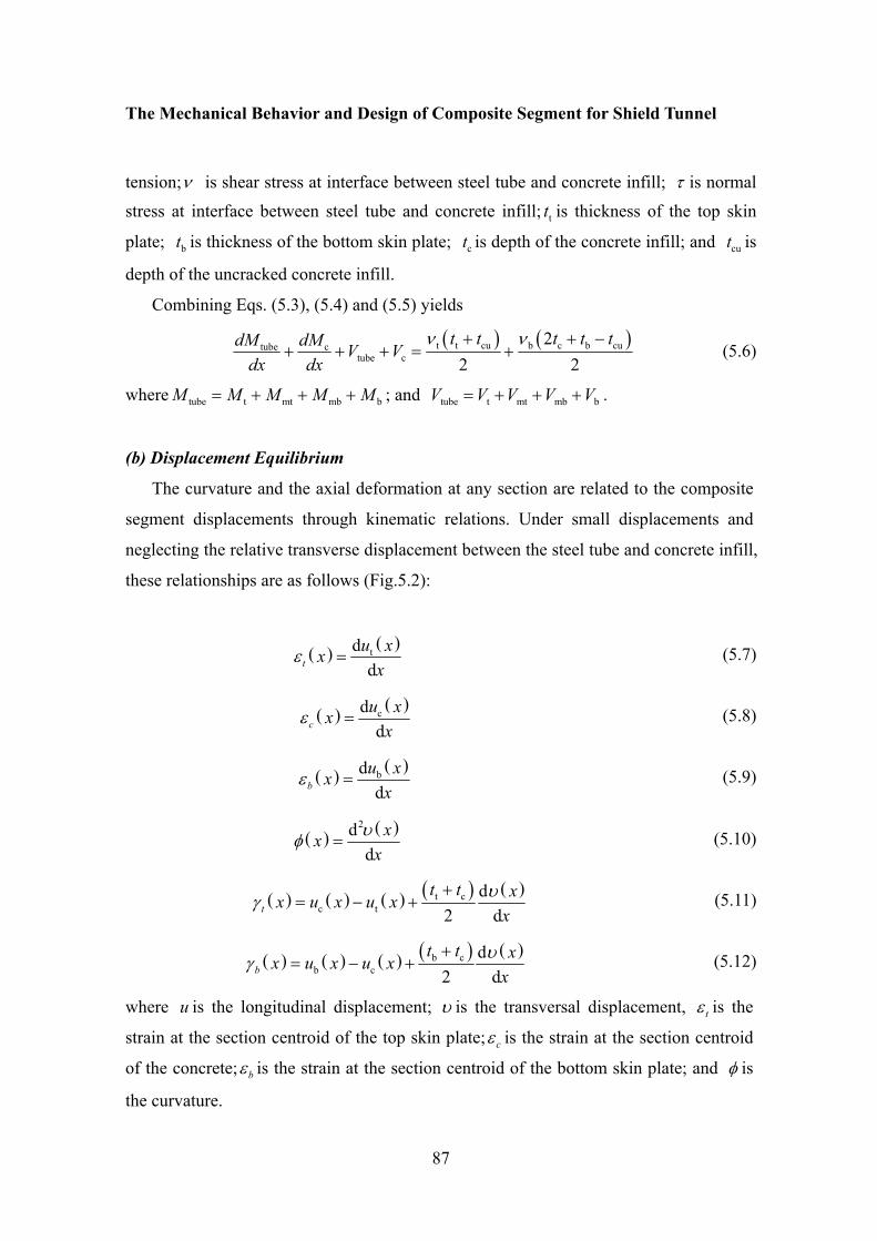
The Mechanical Behavior and Design of Composite Segment for Shield Tunnel
87
tension;ν is shear stress at interface between steel tube and concrete infill; τ is normal stress at interface between steel tube and concrete infill; tt is thickness of the top skin
plate; bt is thickness of the bottom skin plate; ct is depth of the concrete infill; and cut is
depth of the uncracked concrete infill.
Combining Eqs. (5.3), (5.4) and (5.5) yields
( ) ( )t t cu b c b cutube ctube c
22 2
t t t t tdM dM V Vdx dx
ν ν+ + −+ + + = + (5.6)
where tube t mt mb bM M M M M= + + + ; and tube t mt mb bV V V V V= + + + .
(b) Displacement Equilibrium
The curvature and the axial deformation at any section are related to the composite
segment displacements through kinematic relations. Under small displacements and
neglecting the relative transverse displacement between the steel tube and concrete infill,
these relationships are as follows (Fig.5.2):
( ) ( )tddt
u xxx
ε = (5.7)
( ) ( )cddc
u xxx
ε = (5.8)
( ) ( )bddb
u xxx
ε = (5.9)
( ) ( )2dd
xxx
υφ = (5.10)
( ) ( ) ( ) ( ) ( )t cc t
d2 dt
t t xx u x u xx
υγ+
= − + (5.11)
( ) ( ) ( ) ( ) ( )b cb c
d2 db
t t xx u x u xx
υγ+
= − + (5.12)
where u is the longitudinal displacement; υ is the transversal displacement, tε is the
strain at the section centroid of the top skin plate; cε is the strain at the section centroid
of the concrete; bε is the strain at the section centroid of the bottom skin plate; and φ is
the curvature.

A Mechanical Model of Closed-Composite Segment
88
υ
υ
υθ
θ
θ
cu
bu
tu
γ b
γ t
z
y
x
Fig.5.2 Kinematic of composite segment
tcuht
hb
ε
εt2
εct
tttb
tc
Cracked concrete
εt1εc1
εb2εb1
εc2
Uncracked concrete
Fig.5.3 Strain distribution of composite segment
Slip occurs at the interface between steel tube and concrete infill based on the
analysis of experimental data and FEM results in Chapter 3 and Chapter 4 respectively.
Therefore, the rate of change of slip equals the strain difference at the interface and if
tensile strains are assumed positive, the following equations may be derived shown in
Fig.5.3.
The assumption (5) gives
The Mechanical Behavior and Design of Composite Segment for Shield Tunnel
89
t t
t tt
sn Kνγ = (5.13)
b b
b bb
sn Kνγ = (5.14)
where tγ is the top relative slip between the top skin plate and concrete infill; bγ is the
bottom relative slip between the top skin plate and concrete infill; ts is the longitudinal
spacing of the top shear studs; bs is the longitudinal spacing of the bottom shear studs;
tn is number of the top shear studs in a group; bn is number of the top shear studs in a
group; tK is stiffness of a top shear stud; and bK is stiffness of a bottom shear stud.
Taking the derivative with respect to x in Eqs. (5.13) and (5.14) and then using Eqs.
(5.1) and (5.2) gives the differential equations. The relative slip strains at the interface
are calculated as 2
t t mtt2 c12
t t
d d ( )d d
tst
s T Tx n K xγε ε ε+
= = − = − (5.15)
2b b mb
c2 b12b b
d d ( )d d
bsb
s T Tx n K xγε ε ε+
= = − = − (5.16)
Strains at the top skin plate ( t2ε ), the top of the concrete infill ( c1ε ), the bottom of
the concrete infill ( c2ε ), and the bottom skin plate ( b1ε ) are calculated from the bending
and axial force as
t mt t mt tt2
t t m mt t t m mt 2T T M T t
E A E A E I E Iε
⎛ ⎞ ⎛ ⎞+ += − +⎜ ⎟ ⎜ ⎟+ +⎝ ⎠ ⎝ ⎠
(5.17)
c c cuc1
c cu c cu 2T M t
E A E Iε = − − (5.18)
c c cuc2 c
c cu c cu 2T M tt
E A E Iε ⎛ ⎞= − − −⎜ ⎟
⎝ ⎠ (5.19)
b mb b mb bb1
b b m mb b b m mb 2T T M M t
E A E A E I E Iε
⎛ ⎞ ⎛ ⎞+ += −⎜ ⎟ ⎜ ⎟+ +⎝ ⎠ ⎝ ⎠
(5.20)
where tA is area of the top skin plate section; mtA is area of main girder section in
compression; cuA is the uncracked concrete section; bA is the bottom skin plate section;
mbA is main girder section in tension; tE is elastic modulus of the top skin plate; mE is
elastic modulus of main girders; cE is elastic modulus of the concrete infill; bE is
A Mechanical Model of Closed-Composite Segment
90
elastic modulus of the bottom skin plate; tI is moment of inertia of the top skin plate
section; mtI is moment of inertia of main girder section in compression; cuI is moment of
inertia of the uncracked concrete section; mbI is moment of inertia of main girder section
in tension; and bI is moment of inertia of the bottom skin plate section.
The assumption (3) gives
t mt b mb c
t t m mt b b m mb c cu
M T M M ME I E I E I E I E I
φ + += = =
+ + (5.21)
Substituting Eqs. (5.17), (5.18), (5.19), (5.20), and (5.21) into Eqs.(5.15) and (5.16)
gives:
c t mtt
c cu t t m mt
dd
t T T Thx E A E A E Aγ φ
⎛ ⎞+= + − ⎜ ⎟+⎝ ⎠
(5.22)
b mb cb
b b m mb c cu
dd
b T T Thx E A E A E Aγ φ
⎛ ⎞+= − −⎜ ⎟+⎝ ⎠
(5.23)
where ( )t t cu / 2h t t= + ; and ( )b c b cu2 / 2h t t t= + − .
Taking the derivative with respect to x in Eqs. (5.22) and (5.23) and then giving the
following differential equations:
1 1 1t t b Vγ α γ β γ η′′ = − + + (5.24)
2 2 2b b t Vγ α γ β γ η′′ = − + + (5.25)
where 2
t t1
t t t m mt c cu
1 1tn K hs EI E A E A E A
α⎛ ⎞
= + +⎜ ⎟+⎝ ⎠; b t b
1b c cu
1bn K h hs EI E A
β⎛ ⎞
= −⎜ ⎟⎝ ⎠
;
2b b
2b b b m mb c cu
1 1bn K hs EI E A E A E A
α⎛ ⎞
= + +⎜ ⎟+⎝ ⎠; t b t
2t c cu
1tn K h hs EI E A
β⎛ ⎞
= −⎜ ⎟⎝ ⎠
;
t1
hEI
η = ; b2
hEI
η = ;
t t m mt b b m mb c cuEI E I E I E I E I E I= + + + + ; and tube cV V V= + .
The fourth order differential equations for the relative slips, tγ and bγ , are
( ) ( ) ( )(4)1 2 1 2 1 2 2 1 1 2t t t Vγ α α γ α α β β γ α η βη′′+ + − − = + (5.26)
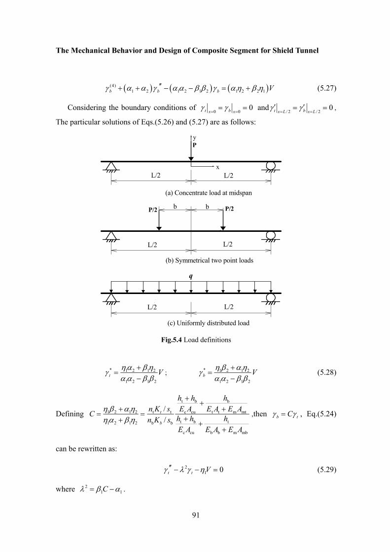
The Mechanical Behavior and Design of Composite Segment for Shield Tunnel
91
( ) ( ) ( )(4)1 2 1 2 1 2 1 2 2 1b b b Vγ α α γ α α β β γ αη β η′′+ + − − = + (5.27)
Considering the boundary conditions of 0 0
0t bx xγ γ
= == = and
/ 2 / 20t bx L x L
γ γ= =
′ ′= = ,
The particular solutions of Eqs.(5.26) and (5.27) are as follows:
x
y
bb
L/2L/2
L/2L/2
L/2L/2
q
P/2 P/2
P
(c) Uniformly distributed load
(b) Symmetrical two point loads
(a) Concentrate load at midspan
Fig.5.4 Load definitions
* 1 2 1 2
1 2 1 2t Vηα βηγ
α α β β+
=−
; * 1 2 1 2
1 2 1 2b Vη β αηγ
α α β β+
=−
(5.28)
Defining
t b b
1 2 1 2 t t c cu t t m mt
t b t1 2 1 2 b b
c cu b b m mb
//
t
b
h h hn K s E A E A E AC h h hn K s
E A E A E A
η β αηηα βη
+ ++ +
= =++ +
+
,then b tCγ γ= , Eq.(5.24)
can be rewritten as:
21 0t t Vγ λ γ η′′ − − = (5.29)
where 21 1Cλ β α= − .
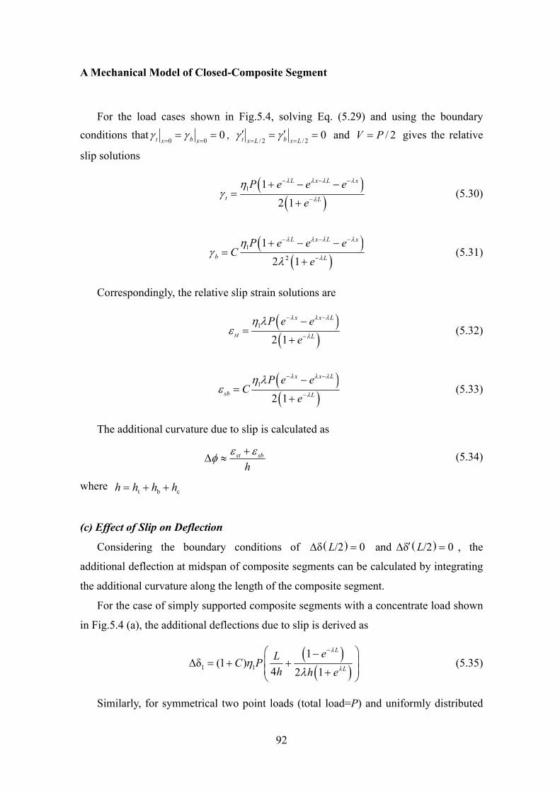
A Mechanical Model of Closed-Composite Segment
92
For the load cases shown in Fig.5.4, solving Eq. (5.29) and using the boundary conditions that
0 00t bx x
γ γ= == = ,
/ 2 / 20t bx L x L
γ γ= =
′ ′= = and / 2V P= gives the relative
slip solutions
( )( )
1 1
2 1
L x L x
t L
P e e e
e
λ λ λ λ
λ
ηγ
− − −
−
+ − −=
+ (5.30)
( )( )
12
1
2 1
L x L x
b L
P e e eC
e
λ λ λ λ
λ
ηγ
λ
− − −
−
+ − −=
+ (5.31)
Correspondingly, the relative slip strain solutions are
( )( )
1
2 1
x x L
st L
P e e
e
λ λ λ
λ
η λε
− −
−
−=
+ (5.32)
( )( )
1
2 1
x x L
sb L
P e eC
e
λ λ λ
λ
η λε
− −
−
−=
+ (5.33)
The additional curvature due to slip is calculated as
st sb
hε εφ +
Δ ≈ (5.34)
where t b ch h h h= + +
(c) Effect of Slip on Deflection
Considering the boundary conditions of ( )δ /2 0LΔ = and ( )δ /2 0L′Δ = , the
additional deflection at midspan of composite segments can be calculated by integrating
the additional curvature along the length of the composite segment.
For the case of simply supported composite segments with a concentrate load shown
in Fig.5.4 (a), the additional deflections due to slip is derived as
( )( )1 1
1δ (1 )
4 2 1
L
L
eLC Ph h e
λ
λη
λ
−⎛ ⎞−⎜ ⎟Δ = + +⎜ ⎟+⎝ ⎠
(5.35)
Similarly, for symmetrical two point loads (total load=P) and uniformly distributed
The Mechanical Behavior and Design of Composite Segment for Shield Tunnel
93
load q shown in Figs. Fig.5.4 (b) and (c), the additional deflections due to slip are
derived, respectively, as
( )2 12δ (1 )
4 2 1
b L b
L
L b e eC Ph h e
λ λ λ
λη
λ
−⎛ ⎞− −Δ = + +⎜ ⎟⎜ ⎟+⎝ ⎠
(5.36)
( )2 ( ) / 2
3 1 2
2 1δ (1 )8 1
L L
L
L e eC qh h e
λ λ
λη
λ⎛ ⎞− −
Δ = + +⎜ ⎟⎜ ⎟+⎝ ⎠ (5.37)
where 1δΔ is additional deflection due to slip for concentrate load; 2δΔ is additional
deflection due to slip for symmetrical two point loads; 3δΔ is additional deflection due to
slip for uniformly distributed load.
The total deflection calculated from elastic deformation and slip-induced deflection
is
( )( )
3
1 1
1δ (1 )
48 4 2 1
L
L
ePL LC PEI h h e
λ
λη
λ
−⎛ ⎞−⎜ ⎟= + + +⎜ ⎟+⎝ ⎠
(5.38)
( )
( )
2
1
δ 2 312 2 2
2(1 )4 2 1
b L b
L
P L Lb b b L bEI
L b e eC Ph h e
λ λ λ
λη
λ
−
⎡ ⎤⎛ ⎞ ⎛ ⎞= − + − −⎜ ⎟ ⎜ ⎟⎢ ⎥⎝ ⎠ ⎝ ⎠⎣ ⎦⎛ ⎞− −
+ + +⎜ ⎟⎜ ⎟+⎝ ⎠
(5.39)
( )4 2 ( ) / 2
3 1 2
5 2 1δ (1 )384 8 1
L L
L
qL L e eC qEI h h e
λ λ
λη
λ⎛ ⎞− −
= + + +⎜ ⎟⎜ ⎟+⎝ ⎠ (5.40)
5.3 MATERIAL MODELS
The material behavior is described using explicit relationships between the total
stress and the total strain with appropriate loading/unloading conditions.
5.3.1 Concrete (a) Unconfined Concrete
The stress-strain relationship suggested by Carreira and Chu [1] is adopted in
A Mechanical Model of Closed-Composite Segment
94
unconfined concrete for compression region. The initial portion of the ascending branch
is linearly elastic, but at about 30% of the ultimate strength, the presence of micro-cracks
leads to a nonlinear behavior, with a reduction in tangent modulus.
1
cc
cc
c
c
f
α
εαε
σεαε
⎛ ⎞′ ⎜ ⎟⎜ ⎟′⎝ ⎠=
⎛ ⎞− + ⎜ ⎟⎜ ⎟′⎝ ⎠
(5.41)
where cσ is compressive stress in concrete( 2N/mm ); cε is strain in concrete; cf ′ is
uniaxial compressive strength of concrete( 2N/mm ); ci2 /c cf Eε ′ ′= ; ciE the initial tangent
modulus of the concrete; and α as a function of uniaxial compressive strength of
concrete cf ′ , can be estimated by the following formula
3
1.55cfαβ′⎡ ⎤
= +⎢ ⎥⎣ ⎦
(5.42)
The coefficient of variability β increases when increasing the compressive strength of
the concrete. Therefore, if 221.0N/mmcf ′ = , 22.0β = and if 280.0N/mmcf ′ = , 71.4β = ,
for intermediate stress gradients, β can be determined by linear interpolations. In tension region, the stress-strain relationship is described by the CEB-FIB Model
Code 90 [2].
ci ci
ci
ci
0 0.9 /
0.1 (0.00015 ) 0.9 / 0.000150.00015 0.9 /
0 0.00015
c c t
tc t c t c
t
c
E f E
ff f Ef E
ε ε
σ ε ε
ε
⎧ ′< ≤⎪
′⎪⎪ ′ ′= − − < ≤⎨ ′−⎪⎪ >⎪⎩
(5.43)
(b) Confined Concrete
In compression region, Montoya et al.[3] proposed a concrete confinement model for steel tube confined concrete is adopted for confined concrete. The stress cσ is related to

The Mechanical Behavior and Design of Composite Segment for Shield Tunnel
95
the strain cε using the following formula:
2
1.0
ccc
c c
cc cc
f
A B Cf f
σε ε
=⎛ ⎞ ⎛ ⎞− + +⎜ ⎟ ⎜ ⎟⎝ ⎠ ⎝ ⎠
(5.44)
where dA k= ;sec
2 ABE
= ; 2sec
ACE
= ; and seccc
cc
fEε
= . The shape factor dk is given by the
following formula:
2
80
14
ccd
cc c
fkε ε
⎛ ⎞= ⎜ ⎟−⎝ ⎠ (5.45)
where cc cc
(17 0.06 ) lc c
fff
ε ε ε ⎛ ⎞′ ′ ′= + − ⎜ ⎟′⎝ ⎠; 80cε is the strain corresponding to 80% of the
peak stress, cc0.80 f ,and given by the following formula:
( )80 1.5 89.5 0.6 lc c c
c
fff
ε ε ⎡ ⎤′ ′= + −⎢ ⎥′⎣ ⎦ (5.46)
Peak axial stress for confined concrete ccf is defined as
cc
c t
1lf ff f
α⎛ ⎞′
= +⎜ ⎟⎜ ⎟′ ′⎝ ⎠ (5.47)
where constantα = given by
( ) 0.21
c
t
1.25 1 0.062 lf ff
α−⎛ ⎞ ′= +⎜ ⎟′⎝ ⎠
(5.48)
and the tensile strength 2 / 3t 0.23( )cf f′ ′= .
The effective lateral pressure lf ′acting on the concrete due to the steel jacket can be
calculated as follows:
l s lf k f′ = (5.49)
A Mechanical Model of Closed-Composite Segment
96
where sk is the effectiveness coefficient representing the ratio of the effectively
confined area to the total cross section area and lf is the possible maximum confining
pressure that exerted by steel jacket on the concrete core. sk and lf can be calculated by
Eqs.(2.8) and (2.6) expressed in Chapter 2 respectively.
In tension region, the above stress-strain relationship proposed by the CEB-FIB
Model Code 90 [2] is adopted.
5.3.2 Steel
In the present study, the steel is modeled as an elastic-plastic material incorporating
strain hardening. Specifically, the relationship is linearly elastic up to yielding, plastic
between the elastic limit and the commencement of strain hardening, linear hardening
occurs up to the ultimate tensile stress shown in Fig.2.1.
However, local buckling occurs on the thin steel plates of concrete infill steel tube
members. In general, local buckling of thin steel plates depends on the plate aspect ratio,
width-to-thickness ratio, applied edge stress gradients, boundary conditions, geometric
imperfections, and residual stresses. According to Guideline of buckling design of JSCE code [5], the post-buckling stress udf ′ is calculated as:
( )/ud s syf t s E f′ = (5.50)
where t is the thickness of the steel plate; s is the longitudinal spacing of shear connectors; sE is the elastic modulus of the steel plate; and syf is the yield strength of
the steel plate.
5.3.3 Reinforcement embedded in concrete
When uncracked concrete is in tension, the tensile force is distributed between the
reinforcement and the concrete in proportion to their respective stiffness, and cracking
occurs when the stress reaches a value corresponding to the tensile strength of the
concrete. In a cracked cross-section all tensile forces are balanced by the steel encased in
the concrete only. However, between adjacent cracks, tensile forces are transmitted from
the steel to the surrounding concrete by bond forces. The contribution of the concrete
may be considered to increase the stiffness of the tensile reinforcement. This effect is
The Mechanical Behavior and Design of Composite Segment for Shield Tunnel
97
called tension-stiffening. To describe this effect, a number of models have been proposed.
The majority of the models are based on the mean axial stress and the mean axial strain
of the concrete member in the reinforced concrete, [5-9].
To take the tension stiffening effect into account, the stress average strain
relationship of steel embedded in concrete proposed by the CEB-FIB model [2] is
considered to describe the behavior of the reinforced concrete members in tension.
According to the CEB-FIB Model Code 90 [2] the mean stress-strain relationship of
embedded steel may be expressed as
( )
( )
( )
, s,m sr1
srn sr1sr1 , sr1 sr1 , srn
srn sr1
srnsrn , srn srn , sry
sry srn
sry , sr,sh
, sry sr,sh , srusru sry
, sru
11 s s m
s m s m
sys m s ms
sy s m
su sysy s m s m
su s m
En
f
ff f
f
f
ε ε ερσ σσ ε ε ε ε εε ε
σσ ε ε ε ε εσ ε ε
ε ε ε
ε ε ε ε εε ε
ε ε
⎧⎛ ⎞+ ≤⎪⎜ ⎟⎝ ⎠⎪
−+ − < ≤
−−
+ − < ≤= ⎨ −
< ≤−
+ − < ≤−
>
⎪⎪⎪⎪⎪
⎪⎪⎪⎪⎪⎪⎪⎩
(5.51)
where n and ρ are the modular ratio and the geometric ratios of reinforcing steel,
respectively; sr1σ is the steel stress in the crack, when the first crack has formed; srnσ is
the steel stress in the crack, when the last crack has formed; sr1ε and sr2ε are the steel
strains at the point of zero slip and at the crack when the cracking forces reach ctf ;
( )srn srn sr2 sr1/ 0.4sEε σ ε ε= − − ;
( )sry sy sr2 sr10.4ε ε ε ε= − − ;
( )sr,sh sh sr2 sr10.4ε ε ε ε= − − ;
( ) ( )sru sr,sh sr10.8 1 / /sy su sy stf f f Eε ε σ= + − − ;
0.01st sE E= .
In the present study, the steel is modeled as an elastic- plastic material incorporating
strain hardening. Specifically, the relationship is linearly elastic up to yielding, plastic
between the elastic limit and the commencement of strain hardening, linear hardening
A Mechanical Model of Closed-Composite Segment
98
occurs up to the ultimate tensile stress shown in Fig.2.1.
5.3.4 Shear stud connector
The constitutive relationship proposed by Ollgaard et al. [10] is considered for the shear stud connector. The analytical relationship between the shear force Q and the slip
δ of a shear stud is given by
( )0.40.70871uQ Q e δ−= − (5.52)
where Q is the applied load(N); δ is the slip of shear stud(mm).
The stiffness at 0.5 uQ was proposed as initial stiffness of a shear stud is given by
( )sh 0.16 0.0017u
si
c
QKd f
=′−
(5.53)
where siK is initial stiffness of a shear stud(N/mm); uQ is shear capacity of a shear stud
accounting for the effects of shear stud spacing and plate thickness, and given by
0.400.65 0.35
sh1.35.3 ( ) c
u V su cs
EQ A f fEn
ηβ⎛ ⎞⎛ ⎞ ′= − ⎜ ⎟⎜ ⎟
⎝ ⎠ ⎝ ⎠ (5.54)
whereη and Vβ are reduction factors of the shear capacity and described in Chapter 2.
5.4 CROSS SECTIONAL ANALYSIS
The procedure followed to predict the flexural behavior of the composite segment
sections is an incremental iterative method with secant stiffness formulation. For the
present numerical procedure, the cross section is divided into a finite number of discrete
layers (fiber model). Because the slip effect causes an equivalent additional moment to
the section, the elastic flexural capacity (corresponding to the first yielding of the
extreme fiber of the section) of the composite segment is reduced. The calculation model
for the additional moment is shown in Fig. 5.5.
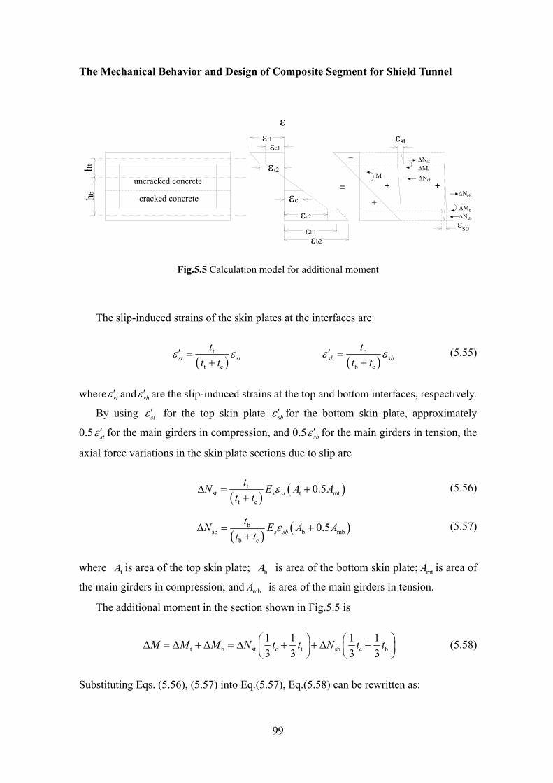
The Mechanical Behavior and Design of Composite Segment for Shield Tunnel
99
hthb
M
+
-
= + +
εsb
εst
ΔNstΔMt
ΔNct
ΔNcb
ΔMbΔNsb
ε
εt2
εct
εt1εc1
εb2εb1
εc2
uncracked concrete
cracked concrete
Fig.5.5 Calculation model for additional moment
The slip-induced strains of the skin plates at the interfaces are
( )t
t cst st
tt t
ε ε′ =+
( )
b
b csb sb
tt t
ε ε′ =+
(5.55)
where stε ′ and sbε ′ are the slip-induced strains at the top and bottom interfaces, respectively.
By using stε ′ for the top skin plate sbε ′ for the bottom skin plate, approximately
0.5 stε ′ for the main girders in compression, and 0.5 sbε ′ for the main girders in tension, the
axial force variations in the skin plate sections due to slip are
( ) ( )tst t mt
t c
0.5s sttN E A A
t tεΔ = +
+ (5.56)
( ) ( )b
sb b mbb c
0.5s sbtN E A A
t tεΔ = +
+ (5.57)
where tA is area of the top skin plate; bA is area of the bottom skin plate; mtA is area of
the main girders in compression; and mbA is area of the main girders in tension.
The additional moment in the section shown in Fig.5.5 is
t b st c t sb c b1 1 1 13 3 3 3
M M M N t t N t t⎛ ⎞ ⎛ ⎞Δ = Δ + Δ = Δ + + Δ +⎜ ⎟ ⎜ ⎟⎝ ⎠ ⎝ ⎠
(5.58)
Substituting Eqs. (5.56), (5.57) into Eq.(5.57), Eq.(5.58) can be rewritten as:
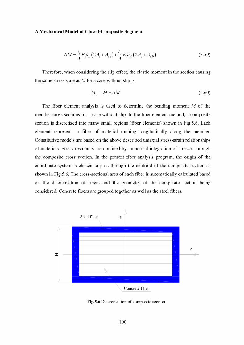
A Mechanical Model of Closed-Composite Segment
100
( ) ( )t bt mt b mb2 2
3 3s st s sbt tM E A A E A Aε εΔ = + + + (5.59)
Therefore, when considering the slip effect, the elastic moment in the section causing
the same stress state as M for a case without slip is
pM M M= − Δ (5.60)
The fiber element analysis is used to determine the bending moment M of the
member cross sections for a case without slip. In the fiber element method, a composite
section is discretized into many small regions (fiber elements) shown in Fig.5.6. Each
element represents a fiber of material running longitudinally along the member.
Constitutive models are based on the above described uniaxial stress-strain relationships
of materials. Stress resultants are obtained by numerical integration of stresses through
the composite cross section. In the present fiber analysis program, the origin of the
coordinate system is chosen to pass through the centroid of the composite section as
shown in Fig.5.6. The cross-sectional area of each fiber is automatically calculated based
on the discretization of fibers and the geometry of the composite section being
considered. Concrete fibers are grouped together as well as the steel fibers.
Steel fiber
Concrete fiber
y
x
H
Fig.5.6 Discretization of composite section
The Mechanical Behavior and Design of Composite Segment for Shield Tunnel
101
Member forces are determined as the stress resultants in a composite section by the
following equations:
, , , ,1 1
ns nc
s i s i c j c ji j
P A Aσ σ= =
= +∑ ∑ (5.61)
, , , ,1 1
ns nc
s i s i i c j c j ji j
M A y A yσ σ= =
= +∑ ∑ (5.62)
where P is the axial force; M is bending moment about the major principal axis; ,s iσ is
the longitudinal stress at centroid of steel fiber i ; ,s iA is is the area of steel fiber
i ; ,c jσ is the longitudinal stress at the centroid of concrete fiber j ; ,c jA is the area of
concrete fiber j ; iy is the coordinates of steel fiber i ; jy is the coordinates of concrete
fiber j ; ns is the total number of steel fiber elements, and nc is the total number of
concrete fiber elements. Compressive stresses are taken to be positive. Stresses in fibers
are calculated using fiber strains and material stress-strain relationships.
In the present method, the proposed secant algorithm by Liang [11] is used in the fiber element analysis program to iterate the depth and orientation of the neutral axis until equilibrium conditions are satisfied. The neutral axis depth ( nd ) is adjusted by using the following equation:
( ), 1 ,, 2 , 1
, 1 ,
n j n jn j n j
p j p j
d dd d
f f+
+ ++
−= −
− (5.63)
where the subscript j is the iteration number; and p nf P P= − , nP is the given axial
load. The convergence criterion for the neutral axis depth nd is defined by
, 1 ,n j n jd d e+ − ≤ (5.64)
where e is the convergence tolerance.
To simplify the calculation of ultimate carrying capacity, it is reasonably assumed
that the effect of transverse reinforcement can be ignored in carrying capacity
calculation. According to the position of the plastic neutral axis in the concrete infill, the
calculation of ultimate carrying capacity is discussed in the following section.

A Mechanical Model of Closed-Composite Segment
102
The strain and stress distributions over the section depth for composite segment are shown in Fig.5.7. The strain in the tension steel, ,s mε at failure is given by:
t b c,
ts m cc
t t t d cd t
ε ε+ + − −=
− (5.65)
where d is the depth of neutral axis; c is the depth of tension steel. For a segment section
with a constant width the parabolic portion of concrete stress distribution can be replaced by an equivalent rectangular block introducing the stress block factors 1α and
1β [12]. The resultant forces of the equivalent rectangular block have the same
magnitude and location as those of the actual parabolic stress distribution.
2cp cp
1 1c c
1 /3
ε εα β
ε ε
⎡ ⎤⎛ ⎞= −⎢ ⎥⎜ ⎟′ ′⎢ ⎥⎝ ⎠⎣ ⎦
(5.66)
cp c1
cp
4 /6 2 / c
ε εβ
ε ε′−
=′−
(5.67)
where cpε is the concrete strain at the end of the parabolic portion of the concrete stress
distribution. At failure, cpε is the ultimate compressive strain of an unconfined concrete
for unconfined segment while for steel tube-confined segment cp cε ε ′= .
tttb
tc
tm
,t1sf
,b1sfAs
c
Main reinforcement
s,mε
b
φ
cc st( )ε ε+
Equivalent Stressdistribution
Concrete
Mai
n gi
rder
Mai
n gi
rder 3d
tf ′tf ′
1 cfα ′
1 1dβcf ′
ccf2d
1d
dccf
cf ′
N.A
ctε
ccε
cε ′
Actual Stress distribution
Steel tubeConcrete
Strain distribution
Skin plate
Concrete infill
Skin plate
Composite section
Fig.5.7 Strain and stress distribution of composite segment
The Mechanical Behavior and Design of Composite Segment for Shield Tunnel
103
At failure, equilibrium conditions are imposed in terms of axial force, uP , and
bending moment, uM .
1 1 1 2 ,t1 t ,t1 t m
3 ,b1 b ,b1 t c m
u
( )2
( )2
cc cc s s
cts s s st
f ff d b d b f t b f d t t
f d b f t b f t t d t A f
P
α β′+′ + + + −
− − − + − −
=
(5.68)
( ) ( )
( )
( )
1 1 1 1 1 1 2 1 2
2,t1 t 1 2 t ,t1 t m
23 ,b1 b t c b
2,b1 t c m t c b
u
0.5 0.52
20.5 ( )3
( 0.5 )3
2 ( )3
cc cc
s s
cts
s s st
f ff d b d d d b d d
f t b d d t f d t t
f d b f t t t t d b
f t t d t A t t t d c f
M
α β β′+′ − + + +
+ + + −
− − + + −
− + − − + + − −
=
(5.69)
where
1
unconfined segment
confined segmentc
cc
dd
d εε
⎧⎪= ′⎛ ⎞⎨
⎜ ⎟⎪ ⎝ ⎠⎩
; 2
0 unconfined segment
1 confined segmentc
cc
dd ε
ε
⎧⎪= ′⎛ ⎞⎨ −⎜ ⎟⎪ ⎝ ⎠⎩
stf is the stress in tension steel; sA is the area of the main reinforcements.
For simplification, uM can be calculated as:
( ) s-t s-bu-tube full-Rd u-tube
s-t s-b1uk kM M M M
k k+
= + −+
(5.70)
where u-tubeM is the ultimate bending moment of steel tube; full-RdM is the ultimate bending
moment of a full composite segment have the same section; and s-tk , s-bk are degrees of
composite action and given by:
{ }d-t
s-tc c-tube
1min ,
FkN N
= ≤ (5.71)
{ }d-b
s-bc b-tube
1min ,
FkN N
= ≤ (5.72)
A Mechanical Model of Closed-Composite Segment
104
where d-t t uF nV ′= ; d-b b uF n V ′= ; cN is the compression force of concrete; c-tubeN is the
compression force of steel tube; b-tubeN is the tension force of steel tube; and uV ′ is the
shear capacity of a shear stud accounting for the effect of the joint plate, and given by:
u u m nnQV Q′ = +⋅
(5.73)
where uQ is the shear capacity of a shear stud accounting for the effects of shear stud
spacing and plate thickness; nQ (Eq.(2.26)) is the shear capacity of a joint plate; m is
the rows of a grouped shear studs; and n is columns of shear studs between the joint plate
and the analysis cross section.
In the performance-based analysis of composite segments under axial load and
bending, moment-curvature responses are obtained by incrementally increasing the
curvature and solving for the corresponding moment value for the given constant axial load ( nP ) and vertical load ( VP ). A set of moment-curvature curves for the composite
section can be generated by incrementally increasing the vertical load ( VP ) from zero to
the maximum value maxP .
The analysis procedure used to predict the composite segment strength can be
summarized as follows:
(1) Discretize the composite section into fine fiber elements.
(2) Set axial fiber strainsε ε= Δ .
(3). the neutral axis depth ( ),1 ,2,n nd d are set to H and H/2, and φ φ= Δ (4) Calculate fiber stresses using stress-strain relationships.
(5) Check local buckling and update steel fiber stresses accordingly. (6) Calculate the vertical force ( VP ) and bending moment ( nM ) that satisfy equilibrium
requirements.
(7). Adjust the depth of the neutral axis ( d ) using Eq. (5.64).
(8) Repeat Steps (3)-(7) until , 1 ,n j n jd d e+ − < .
(9) Using the Eq.(5.69) to calculate maxφ .
(11) if maxφ φ< , increase the vertical load by φ φ φ= + Δ , where max /100φ φΔ =
(12) Repeat Steps (3)-(11) until maxM
(13) Calculate the vertical force ( maxP ) and bending moment ( maxM ).
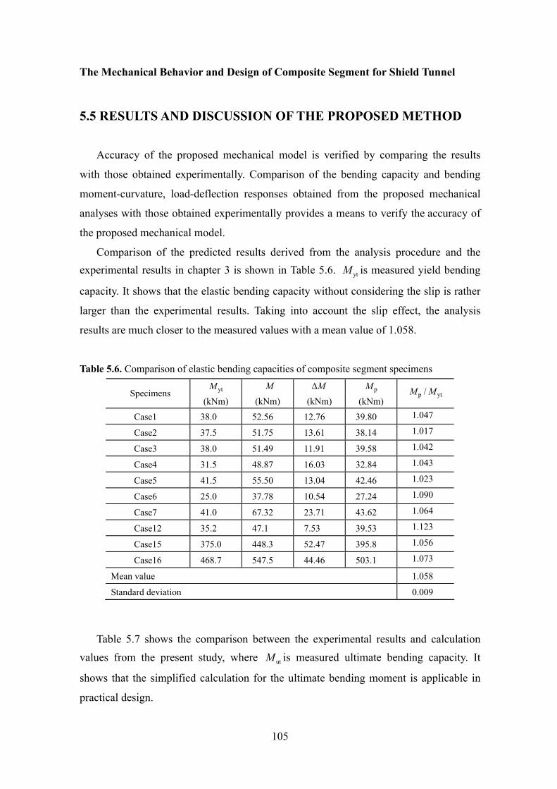
The Mechanical Behavior and Design of Composite Segment for Shield Tunnel
105
5.5 RESULTS AND DISCUSSION OF THE PROPOSED METHOD
Accuracy of the proposed mechanical model is verified by comparing the results
with those obtained experimentally. Comparison of the bending capacity and bending
moment-curvature, load-deflection responses obtained from the proposed mechanical
analyses with those obtained experimentally provides a means to verify the accuracy of
the proposed mechanical model.
Comparison of the predicted results derived from the analysis procedure and the experimental results in chapter 3 is shown in Table 5.6. ytM is measured yield bending
capacity. It shows that the elastic bending capacity without considering the slip is rather
larger than the experimental results. Taking into account the slip effect, the analysis
results are much closer to the measured values with a mean value of 1.058.
Table 5.6. Comparison of elastic bending capacities of composite segment specimens
Specimens ytM (kNm)
M (kNm)
MΔ (kNm)
pM (kNm)
p yt/M M
Case1 38.0 52.56 12.76 39.80 1.047
Case2 37.5 51.75 13.61 38.14 1.017
Case3 38.0 51.49 11.91 39.58 1.042
Case4 31.5 48.87 16.03 32.84 1.043
Case5 41.5 55.50 13.04 42.46 1.023
Case6 25.0 37.78 10.54 27.24 1.090
Case7 41.0 67.32 23.71 43.62 1.064
Case12 35.2 47.1 7.53 39.53 1.123
Case15 375.0 448.3 52.47 395.8 1.056
Case16 468.7 547.5 44.46 503.1 1.073
Mean value 1.058
Standard deviation 0.009
Table 5.7 shows the comparison between the experimental results and calculation values from the present study, where utM is measured ultimate bending capacity. It
shows that the simplified calculation for the ultimate bending moment is applicable in
practical design.
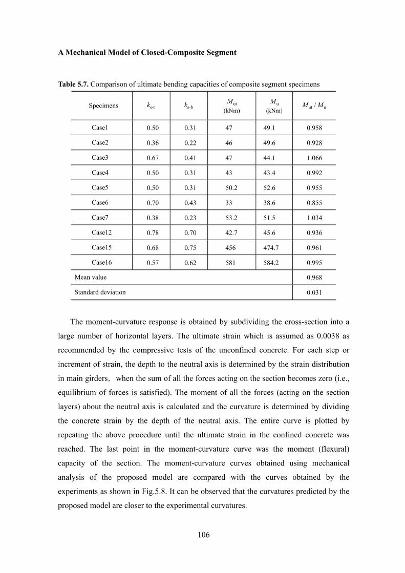
A Mechanical Model of Closed-Composite Segment
106
Table 5.7. Comparison of ultimate bending capacities of composite segment specimens
Specimens s-tk s-bk utM (kNm)
uM (kNm) ut u/M M
Case1 0.50 0.31 47 49.1 0.958
Case2 0.36 0.22 46 49.6 0.928
Case3 0.67 0.41 47 44.1 1.066
Case4 0.50 0.31 43 43.4 0.992
Case5 0.50 0.31 50.2 52.6 0.955
Case6 0.70 0.43 33 38.6 0.855
Case7 0.38 0.23 53.2 51.5 1.034
Case12 0.78 0.70 42.7 45.6 0.936
Case15 0.68 0.75 456 474.7 0.961
Case16 0.57 0.62 581 584.2 0.995
Mean value 0.968
Standard deviation 0.031
The moment-curvature response is obtained by subdividing the cross-section into a
large number of horizontal layers. The ultimate strain which is assumed as 0.0038 as
recommended by the compressive tests of the unconfined concrete. For each step or
increment of strain, the depth to the neutral axis is determined by the strain distribution
in main girders,when the sum of all the forces acting on the section becomes zero (i.e.,
equilibrium of forces is satisfied). The moment of all the forces (acting on the section
layers) about the neutral axis is calculated and the curvature is determined by dividing
the concrete strain by the depth of the neutral axis. The entire curve is plotted by
repeating the above procedure until the ultimate strain in the confined concrete was
reached. The last point in the moment-curvature curve was the moment (flexural)
capacity of the section. The moment-curvature curves obtained using mechanical
analysis of the proposed model are compared with the curves obtained by the
experiments as shown in Fig.5.8. It can be observed that the curvatures predicted by the
proposed model are closer to the experimental curvatures.
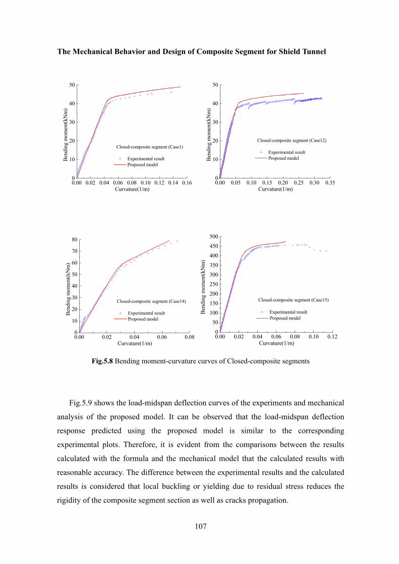
The Mechanical Behavior and Design of Composite Segment for Shield Tunnel
107
0.00 0.02 0.04 0.06 0.08 0.10 0.12 0.14 0.160
10
20
30
40
50
Bend
ing
mom
ent(k
Nm
)
Curvature(1/m)
Closed-composite segment (Case1)
Experimental result Proposed model
0.00 0.05 0.10 0.15 0.20 0.25 0.30 0.350
10
20
30
40
50
Bend
ing
mom
ent(k
Nm
)
Curvature(1/m)
Closed-composite segment (Case12)
Experimental result Proposed model
0.00 0.02 0.04 0.06 0.080
10
20
30
40
50
60
70
80
Bend
ing
mom
ent(k
Nm
)
Curvature(1/m)
Closed-composite segment (Case14)
Experimental result Proposed model
0.00 0.02 0.04 0.06 0.08 0.10 0.120
50
100150
200
250
300
350400
450500
Bend
ing
mom
ent(k
Nm
)
Curvature(1/m)
Closed-composite segment (Case15)
Experimental result Proposed model
Fig.5.8 Bending moment-curvature curves of Closed-composite segments
Fig.5.9 shows the load-midspan deflection curves of the experiments and mechanical
analysis of the proposed model. It can be observed that the load-midspan deflection
response predicted using the proposed model is similar to the corresponding
experimental plots. Therefore, it is evident from the comparisons between the results
calculated with the formula and the mechanical model that the calculated results with
reasonable accuracy. The difference between the experimental results and the calculated
results is considered that local buckling or yielding due to residual stress reduces the
rigidity of the composite segment section as well as cracks propagation.
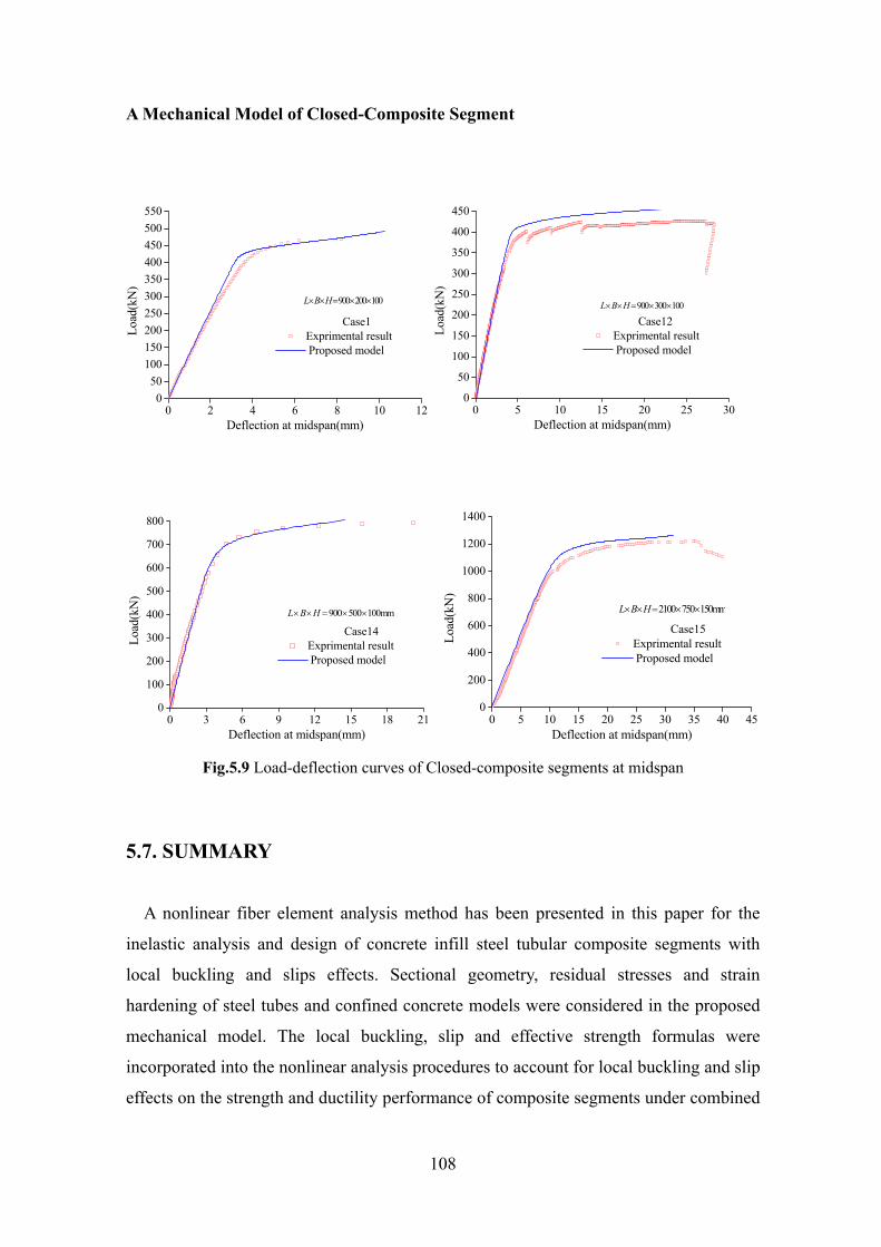
A Mechanical Model of Closed-Composite Segment
108
0 2 4 6 8 10 120
50100150200250300350400450500550
900 200 100L B H× × = × ×
Load
(kN
)
Deflection at midspan(mm)
Case1Exprimental result Proposed model
0 5 10 15 20 25 300
50
100
150
200
250
300
350
400
450
900 300 100L B H× × = × ×
Load
(kN
)Deflection at midspan(mm)
Case12Exprimental result Proposed model
0 3 6 9 12 15 18 210
100
200
300
400
500
600
700
800
900 500 100mmL B H× × = × ×
Load
(kN
)
Deflection at midspan(mm)
Case14Exprimental result Proposed model
0 5 10 15 20 25 30 35 40 45
0
200
400
600
800
1000
1200
1400
2100 750 150mmL B H× × = × ×
Load
(kN
)
Deflection at midspan(mm)
Case15Exprimental result Proposed model
Fig.5.9 Load-deflection curves of Closed-composite segments at midspan
5.7. SUMMARY
A nonlinear fiber element analysis method has been presented in this paper for the
inelastic analysis and design of concrete infill steel tubular composite segments with
local buckling and slips effects. Sectional geometry, residual stresses and strain
hardening of steel tubes and confined concrete models were considered in the proposed
mechanical model. The local buckling, slip and effective strength formulas were
incorporated into the nonlinear analysis procedures to account for local buckling and slip
effects on the strength and ductility performance of composite segments under combined
The Mechanical Behavior and Design of Composite Segment for Shield Tunnel
109
loads.
This paper has presented the formulation of differential equations suitable for the
solution of partially interactive steel tube composite segment elements. Closed form
solutions for single, double and uniform load arrangements on simple span segments
have been presented. A step-wise linearization method has been described which allows
the non-linear affects of concrete cracking and shear stud stiffness to be incorporated.
The analysis involves non-dimensional constants which affect the steel plate
interaction. The effects are either direct when the constant relates to the plate for which
it is formulated or crossed when it affects the opposite plate for which it is formulated.
More attention should be paid on the shear capacity of shear studs in composite
segments. In current codes, only some coefficients are suggested for considering the
influences of the concrete strength, steel strength, and shear stud dimension. It was
found that the shear stud spacing and the thickness of the welded steel plate also have the effects on the shear capacity, so the coefficients η and Vβ are recommended.
Stopping criteria are required to terminate the iterative analysis process once
satisfactory solutions are obtained. In calculating the ultimate axial load of a composite
segment, the analysis may be stopped when axial strain in concrete exceeds the strain
corresponding to the peak stress of unconfined concrete or confined concrete. The
moment-curvature calculations may be stopped when the strain in steel exceeds the
specified ultimate strain or the strain in concrete exceeds the strain corresponding to the
peak stress of unconfined concrete or confined concrete.
Comparisons have been made between experimental results and the mechanical
predictions of behavior using the proposed method. Good agreement has been found and
this indicates that the method is suitable for general analysis of tunnel lining of
composite segment.
5.8. REFERENCES
1) Carreira, D. J., K.H. Chu,1985. Stress-strain relationship for plain concrete in
compression. J., Proc., ACI, 82(11), 797-804.
2) CEB-FIP model code 1990,1991. Lausanne (Switzerland): Comité Euro-International
A Mechanical Model of Closed-Composite Segment
110
du Béton.
3) Montoya, E.,2003. Behavior and analysis of confined concrete. Ph.D. thesis, Univ. of
Toronto, Toronto.
4) Scanlon A, Murray DW, 1974. Time dependent deflections of reinforced concrete slab
deflections. Journal of the Structural Division,100(9):1911-1924.
5) JSCE, 2005. Buckling design guideline.
6) Lin CS, Scordelis AC,1975. Nonlinear analysis of RC shells of general form. Journal
of the Structural Division;101(3):523-538.
7) Vebo A, Ghali A,1977. Moment curvature relation of reinforced concrete slabs.
Journal of the Structural Division,103(3),515-531.
8) Gilbert R, Warner R,1978. Tension stiffening in reinforced concrete slabs. Journal of
the Structural Division,104(12):1885-1900.
9) Q.H. Nguyen et al.,2009. Analysis of composite beams in the hogging moment
regions using a mixed finite element formulation. Journal of Constructional Steel
Research 65, 737-748.
10) Oehlers DJ, Sved G.,1995. Composite beams with limited-slip-capacity shear
connectors. J Struct Eng.,32-38.
11) Qing Quan Liang, 2008. Nonlinear analysis of short concrete-filled steel tubular
beam-columns under axial load and biaxial bending. Journal of Constructional Steel
Research 64, 295-304.
12) Collins MP, Mitchell D. Prestressed concrete basics; 1987. Ottawa,ON, Canada:
Canadian Prestressed Concrete Institute (CPCI).
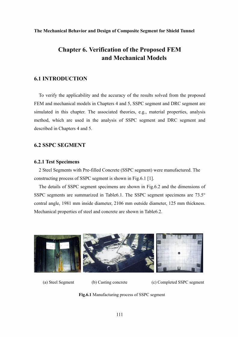
The Mechanical Behavior and Design of Composite Segment for Shield Tunnel
111
Chapter 6. Verification of the Proposed FEM and Mechanical Models
6.1 INTRODUCTION
To verify the applicability and the accuracy of the results solved from the proposed
FEM and mechanical models in Chapters 4 and 5, SSPC segment and DRC segment are
simulated in this chapter. The associated theories, e.g., material properties, analysis
method, which are used in the analysis of SSPC segment and DRC segment and
described in Chapters 4 and 5.
6.2 SSPC SEGMENT
6.2.1 Test Specimens 2 Steel Segments with Pre-filled Concrete (SSPC segment) were manufactured. The
constructing process of SSPC segment is shown in Fig.6.1 [1].
The details of SSPC segment specimens are shown in Fig.6.2 and the dimensions of
SSPC segments are summarized in Table6.1. The SSPC segment specimens are 73.5°
central angle, 1981 mm inside diameter, 2106 mm outside diameter, 125 mm thickness.
Mechanical properties of steel and concrete are shown in Table6.2.
(a) Steel Segment (b) Casting concrete (c) Completed SSPC segment
Fig.6.1 Manufacturing process of SSPC segment

Verification of the Proposed FEM and Mechanical Models
112
Joint plate
Skin plate
Rib
8.0
938.0
3.0125
73.5o
Fig.6.2 Detail of SSPC segment specimen
Table 6.1. Details of SSPC segment specimens
Dimension Thickness Rib
Skin plate
Main girder
Joint plate Specimen Width
(mm)
inside diameter
(mm)
outside diameter
(mm)
central angle
(degree) ts(mm) tm(mm) tj(mm)
Height (mm)
Thickness(mm)
SSPC(Positive bending ) 1000 1981 2106 73.5 3.0 8.0 8.0 93.0 8.0
SSPC(Negative bending ) 1000 1981 2106 73.5 3.0 8.0 8.0 93.0 8.0
Note: Positive bending is the load applied on the outside (ground side) of SSPC; Negative bending is the load applied on the inside (tunnel side) of SSPC.
Table 6.2. Mechanical material properties for SSPC segment specimens
Structural steel Concrete
Specimen Yield strength
2(N/mm )yf
Tensile strength
2(N/mm )sf ′
Young modulus
2(N/mm )sE
Compressive strength
2(N/mm )cf ′
Young modulus
2(N/mm )cE
SSPC 363 570 2.0×10⁵ 27.9 2.3×10⁴

The Mechanical Behavior and Design of Composite Segment for Shield Tunnel
113
6.2.2 Test Setup The simply supported SSPC segment specimens were loaded symmetrically at four
points within the span using a spreader beam shown in Fig.6.3. In these test
arrangements, such loading led, in theory, positive and negative pure bending between
applied forces of the composite segment specimens can be obtained between the two
loading points without the presence of shear and axial forces. The applied load was
measured and recorded using a load cell. The loads were increased gradually with an
increment of approximately 5kN until the ultimate carrying capacities of SSPC segment
specimens. Displacement transducers and Strain gauges located on the key points shown
in Fig.6.4 were used to measure strains and deflections respectively.
SSPC segment
CL
Spreader beam
Load cellP
300
1113.3
Unit:mm
Roller support(hinged and movable)
(a)Test setup for positive bending
SSPC segment
CLLoad cellP
300
1116.7
Unit:mm
Roller support(hinged and movable)
Spreader beam
(b)Test setup for negative bending Fig. 6.3 Test setup for SSPC segment specimens
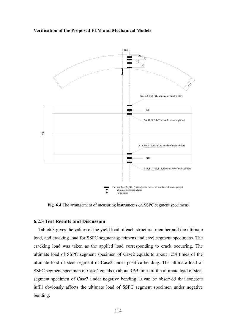
Verification of the Proposed FEM and Mechanical Models
114
S2,S3,S4,S5 (The outside of main girder)
20
20
30
40
100
S6,S7,S8,S9 (The inside of main girder)
S1
S15,S16,S17,S18 (The inside of main girder)
S11,S12,S13,S14(The outside of main girder)
S10
1200
The numbers S1,S2,S3 etc. denote the serial numbers of strain gauges :displacement transducer Unit : mm
125
Fig. 6.4 The arrangement of measuring instruments on SSPC segment specimens
6.2.3 Test Results and Discussion Table6.3 gives the values of the yield load of each structural member and the ultimate
load, and cracking load for SSPC segment specimens and steel segment specimens. The
cracking load was taken as the applied load corresponding to crack occurring. The
ultimate load of SSPC segment specimen of Case2 equals to about 1.54 times of the
ultimate load of steel segment of Case2 under positive bending. The ultimate load of
SSPC segment specimen of Case4 equals to about 3.69 times of the ultimate load of steel
segment specimen of Case3 under negative bending. It can be observed that concrete
infill obviously affects the ultimate load of SSPC segment specimen under negative
bending.
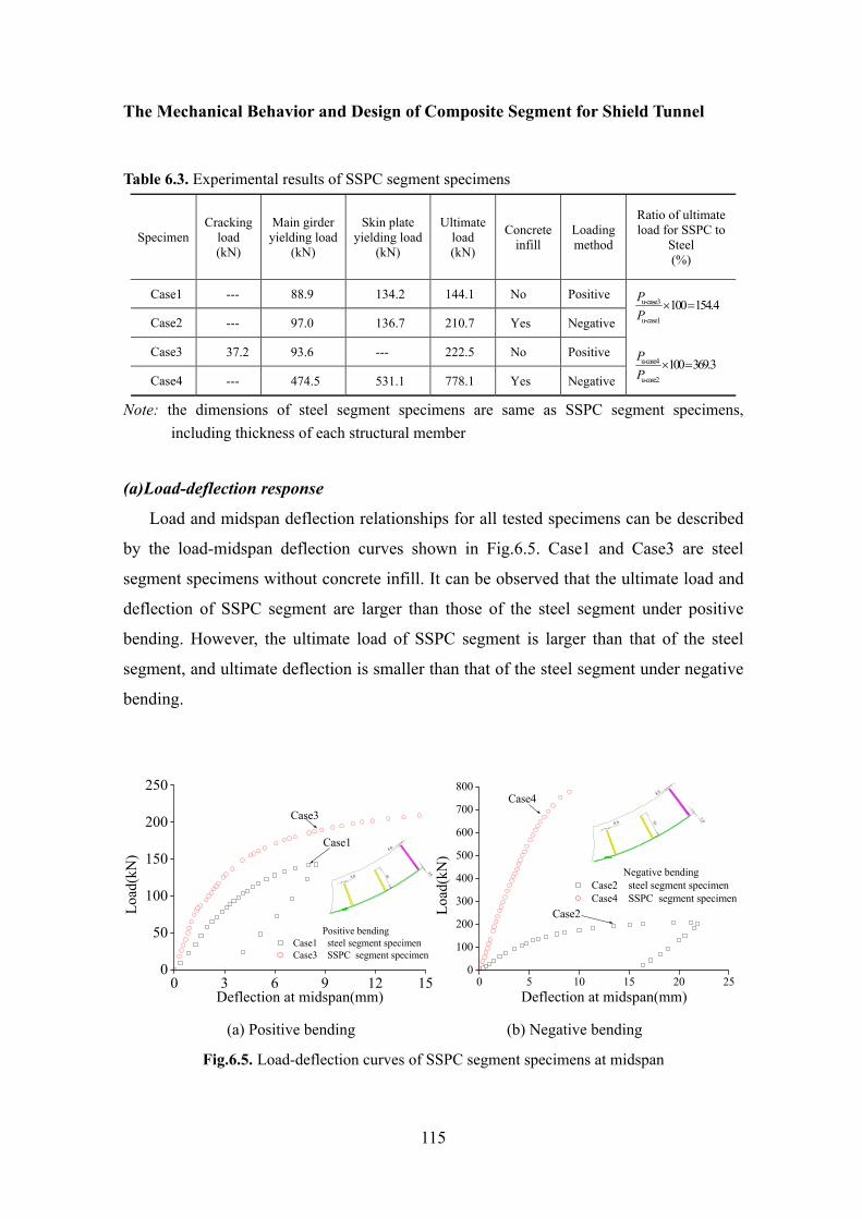
The Mechanical Behavior and Design of Composite Segment for Shield Tunnel
115
Table 6.3. Experimental results of SSPC segment specimens
Specimen Cracking
load (kN)
Main girder yielding load
(kN)
Skin plate yielding load
(kN)
Ultimate load (kN)
Concrete infill
Loading method
Ratio of ultimate load for SSPC to
Steel (%)
Case1 --- 88.9 134.2 144.1 No Positive
Case2 --- 97.0 136.7 210.7 Yes Negative
Case3 37.2 93.6 --- 222.5 No Positive
Case4 --- 474.5 531.1 778.1 Yes Negative
u-case3
u-case1
100 154.4PP
× =
u-case4
u-case2
100 369.3PP
× =
Note: the dimensions of steel segment specimens are same as SSPC segment specimens, including thickness of each structural member
(a)Load-deflection response
Load and midspan deflection relationships for all tested specimens can be described
by the load-midspan deflection curves shown in Fig.6.5. Case1 and Case3 are steel
segment specimens without concrete infill. It can be observed that the ultimate load and
deflection of SSPC segment are larger than those of the steel segment under positive
bending. However, the ultimate load of SSPC segment is larger than that of the steel
segment, and ultimate deflection is smaller than that of the steel segment under negative
bending.
0 3 6 9 12 150
50
100
150
200
250
8.0
938.0
3.0
Case1
Case3
Load
(kN
)
Deflection at midspan(mm)
Positive bendingCase1 steel segment specimenCase3 SSPC segment specimen
0 5 10 15 20 250
100
200
300
400
500
600
700
8008.0
938.0
3.0
Case2
Case4
Load
(kN
)
Deflection at midspan(mm)
Negative bendingCase2 steel segment specimenCase4 SSPC segment specimen
(a) Positive bending (b) Negative bending
Fig.6.5. Load-deflection curves of SSPC segment specimens at midspan

Verification of the Proposed FEM and Mechanical Models
116
(b)Strain distribution
Fig.6.6 shows the measured strain distribution along SSPC segment height (with the
origin at the edge of the main girder to tunnel side) on the double sides of the main
girders. Such curves are displayed under different loading levels for the sections of the
100mm distance from the midspan section. The strain values for the main girders were
taken as the average strain values (from the measured strain based on the
symmetrically-installed strain gauges in the sections of the 100mm distance from the
midspan section). It can be observed that the plane sections remain plane after loading,
because the strain distribution along the height main girder is linear, if the strain values
of the origin are neglected.
-1200 0 1200 2400 3600 4800
0
20
40
60
80
100
120
S2,S3,S4,S5 (The outside of main girder)
2020
30
40
100
S6,S7,S8,S9 (The inside of main girder)
S1,S10
S15,S16,S17,S18 (The inside of main girder)
S11,S12,S13,S14(The outside of main girder)
24.5kN 49.0kN 73.5kN 88.2kN 122.5kN
Case1
Hei
ght o
f mai
n gi
rder
(mm
)
ground side
Microstrain
-1200 0 1200 2400 3600 4800
0
20
40
60
80
100
120
S2,S3,S4,S5 (The outside of main girder)
2020
30
40
100
S6,S7,S8,S9 (The inside of main girder)
S1,S10
S15,S16,S17,S18 (The inside of main girder)
S11,S12,S13,S14(The outside of main girder)
ground side
24.5kN 49.0kN 73.5kN 122.5kN 147.0kN
Case3 with concrete infill
Hei
ght o
f mai
n gi
rder
(mm
)
Microstrain
(a) Positive bending
-3000 -2500 -2000 -1500 -1000 -500 0 500 1000 1500120
100
80
60
40
20
0
-20
S2,S3,S4,S5 (The outside of main girder)
100
S6,S7,S8,S9 (The inside of main girder)
S1,S10
S15,S16,S17,S18 (The inside of main girder)
S11,S12,S13,S14(The outside of main girder)
202030
40
24.5kN 49.0kN 73.5kN 88.2kN 117.6kN
Case2
Hei
ght o
f mai
n gi
rder
(mm
)
Tunnel side
Microstrain
-1500 -1000 -500 0 500 1000120
100
80
60
40
20
0
S2,S3,S4,S5 (The outside of main girder)
100
S6,S7,S8,S9 (The inside of main girder)
S1,S10
S15,S16,S17,S18 (The inside of main girder)
S11,S12,S13,S14(The outside of main girder)
202030
40
58.8kN 96.0kN 156.8kN 196.0kN 264.6kN 294.0kN 343.0kN
Case4 with concrete infill
Hei
ght o
f mai
n gi
rder
(mm
)
Tunnel side
Microstrain
(b) Negative bending Fig.6.6. Measured strain distribution along the height main girder
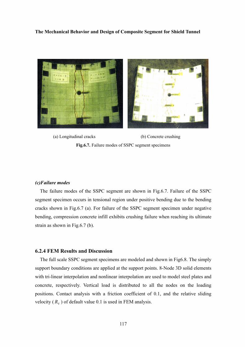
The Mechanical Behavior and Design of Composite Segment for Shield Tunnel
117
(a) Longitudinal cracks (b) Concrete crushing
Fig.6.7. Failure modes of SSPC segment specimens
(c)Failure modes
The failure modes of the SSPC segment are shown in Fig.6.7. Failure of the SSPC
segment specimen occurs in tensional region under positive bending due to the bending
cracks shown in Fig.6.7 (a). For failure of the SSPC segment specimen under negative
bending, compression concrete infill exhibits crushing failure when reaching its ultimate
strain as shown in Fig.6.7 (b).
6.2.4 FEM Results and Discussion The full scale SSPC segment specimens are modeled and shown in Fig6.8. The simply
support boundary conditions are applied at the support points. 8-Node 3D solid elements
with tri-linear interpolation and nonlinear interpolation are used to model steel plates and
concrete, respectively. Vertical load is distributed to all the nodes on the loading
positions. Contact analysis with a friction coefficient of 0.1, and the relative sliding velocity ( VR ) of default value 0.1 is used in FEM analysis.

Verification of the Proposed FEM and Mechanical Models
118
(a) Steel segment (b) FEM model of steel segment
(c) SSPC segment (d) FEM model of SSPC segment
(e) Negative bending (f) Positive bending
Fig.6.8 Finite element model of an SSPC segment
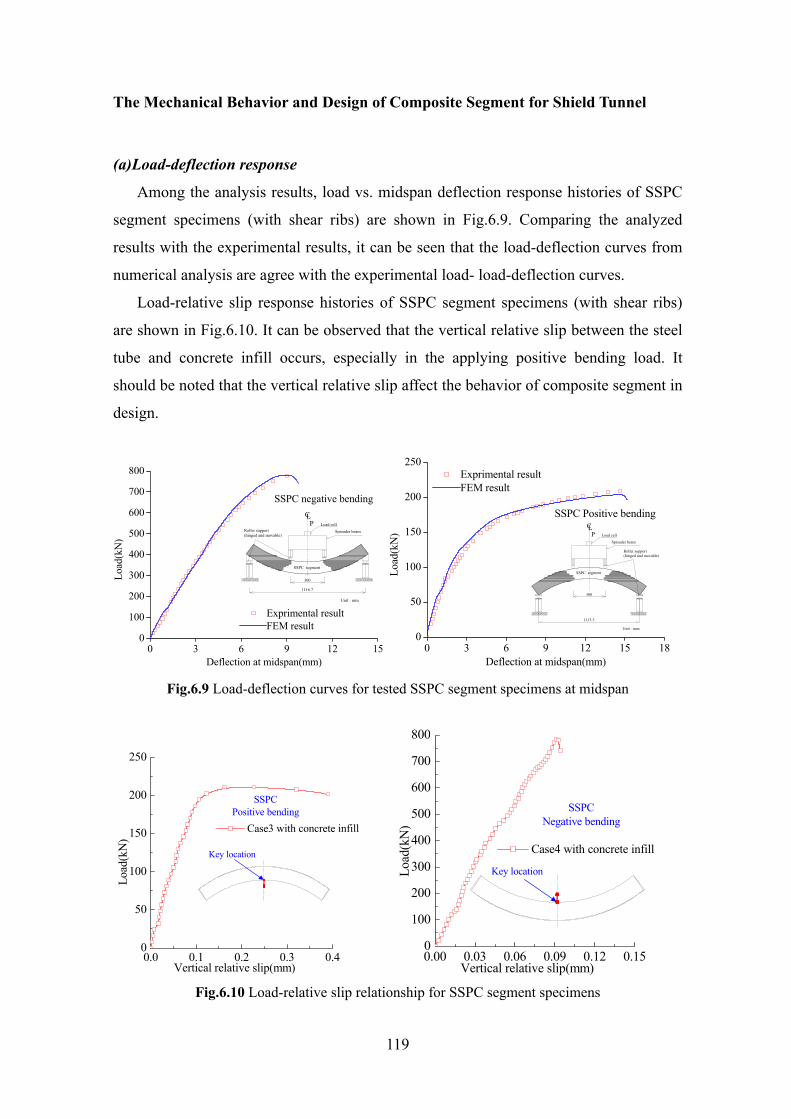
The Mechanical Behavior and Design of Composite Segment for Shield Tunnel
119
(a)Load-deflection response
Among the analysis results, load vs. midspan deflection response histories of SSPC
segment specimens (with shear ribs) are shown in Fig.6.9. Comparing the analyzed
results with the experimental results, it can be seen that the load-deflection curves from
numerical analysis are agree with the experimental load- load-deflection curves.
Load-relative slip response histories of SSPC segment specimens (with shear ribs)
are shown in Fig.6.10. It can be observed that the vertical relative slip between the steel
tube and concrete infill occurs, especially in the applying positive bending load. It
should be noted that the vertical relative slip affect the behavior of composite segment in
design.
0 3 6 9 12 150
100
200
300
400
500
600
700
800
SSPC segment
CLLoad cellP
300
1116.7
Unit:mm
Roller support(hinged and movable)
Spreader beam
SSPC negative bending
Load
(kN
)
Deflection at midspan(mm)
Exprimental result FEM result
0 3 6 9 12 15 180
50
100
150
200
250
SSPC segment
CL
Spreader beam
Load cellP
300
1113.3
Unit:mm
Roller support(hinged and movable)
SSPC Positive bending
Load
(kN
)
Deflection at midspan(mm)
Exprimental result FEM result
Fig.6.9 Load-deflection curves for tested SSPC segment specimens at midspan
0.0 0.1 0.2 0.3 0.40
50
100
150
200
250
Key location
Case3 with concrete infill
SSPCPositive bending
Lo
ad(k
N)
Vertical relative slip(mm)
0.00 0.03 0.06 0.09 0.12 0.150
100
200
300
400
500
600
700
800
Key location
Case4 with concrete infill
SSPCNegative bending
Lo
ad(k
N)
Vertical relative slip(mm)
Fig.6.10 Load-relative slip relationship for SSPC segment specimens
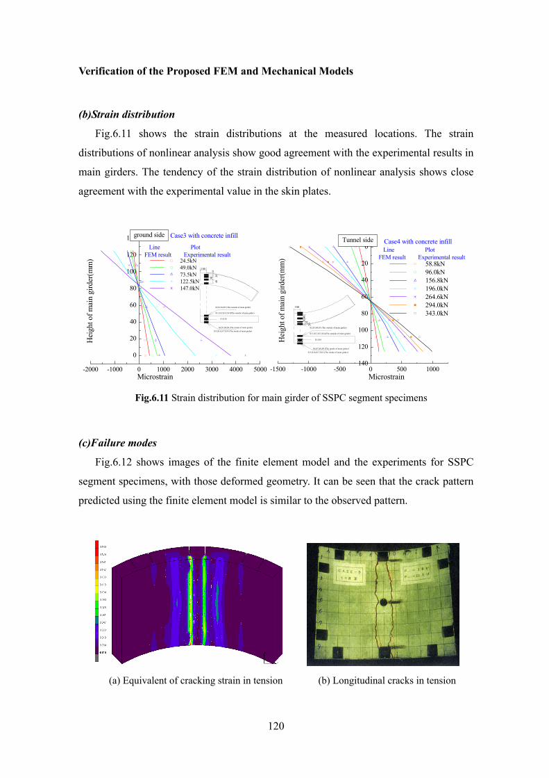
Verification of the Proposed FEM and Mechanical Models
120
(b)Strain distribution
Fig.6.11 shows the strain distributions at the measured locations. The strain
distributions of nonlinear analysis show good agreement with the experimental results in
main girders. The tendency of the strain distribution of nonlinear analysis shows close
agreement with the experimental value in the skin plates.
-2000 -1000 0 1000 2000 3000 4000 5000
0
20
40
60
80
100
120
140 Line PlotFEM result Experimental result
S2,S3,S4,S5 (The outside of main girder)
2020
30
40
100
S6,S7,S8,S9 (The inside of main girder)
S1,S10
S15,S16,S17,S18 (The inside of main girder)
S11,S12,S13,S14(The outside of main girder)
ground side
24.5kN 49.0kN 73.5kN 122.5kN 147.0kN
Case3 with concrete infill
Hei
ght o
f mai
n gi
rder
(mm
)
Microstrain
-1500 -1000 -500 0 500 1000140
120
100
80
60
40
20
0 Line PlotFEM result Experimental result
S2,S3,S4,S5 (The outside of main girder)
100
S6,S7,S8,S9 (The inside of main girder)
S1,S10
S15,S16,S17,S18 (The inside of main girder)
S11,S12,S13,S14(The outside of main girder)
202030
40
58.8kN 96.0kN 156.8kN 196.0kN 264.6kN 294.0kN 343.0kN
Case4 with concrete infill
Hei
ght o
f mai
n gi
rder
(mm
)
Tunnel side
Microstrain
Fig.6.11 Strain distribution for main girder of SSPC segment specimens
(c)Failure modes
Fig.6.12 shows images of the finite element model and the experiments for SSPC
segment specimens, with those deformed geometry. It can be seen that the crack pattern
predicted using the finite element model is similar to the observed pattern.
(a) Equivalent of cracking strain in tension (b) Longitudinal cracks in tension
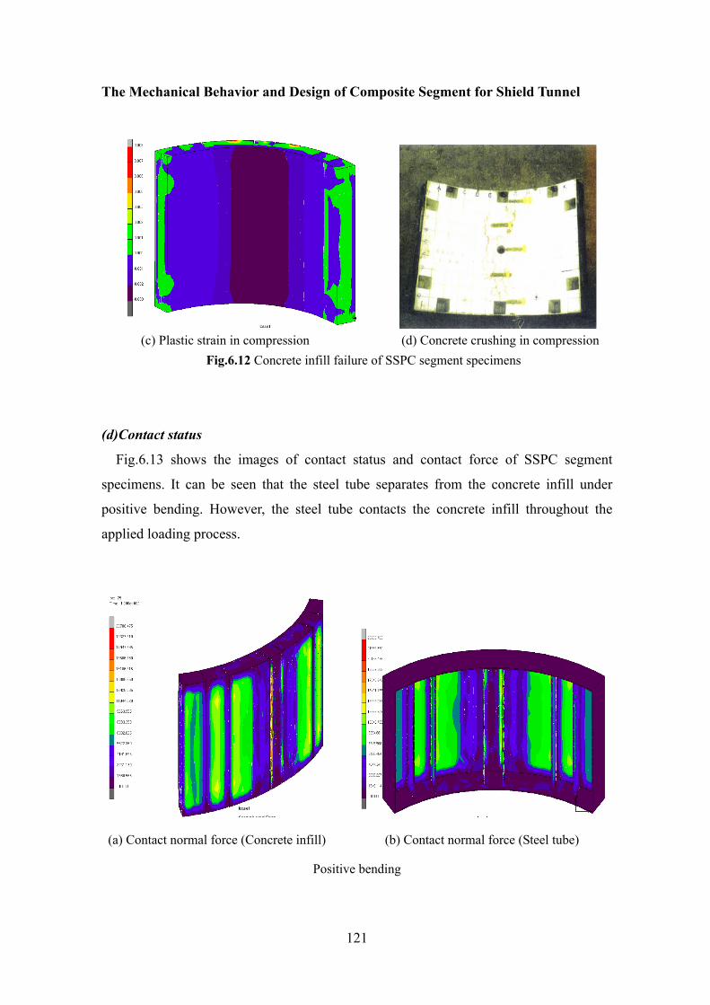
The Mechanical Behavior and Design of Composite Segment for Shield Tunnel
121
(c) Plastic strain in compression (d) Concrete crushing in compression
Fig.6.12 Concrete infill failure of SSPC segment specimens
(d)Contact status
Fig.6.13 shows the images of contact status and contact force of SSPC segment
specimens. It can be seen that the steel tube separates from the concrete infill under
positive bending. However, the steel tube contacts the concrete infill throughout the
applied loading process.
(a) Contact normal force (Concrete infill) (b) Contact normal force (Steel tube)
Positive bending
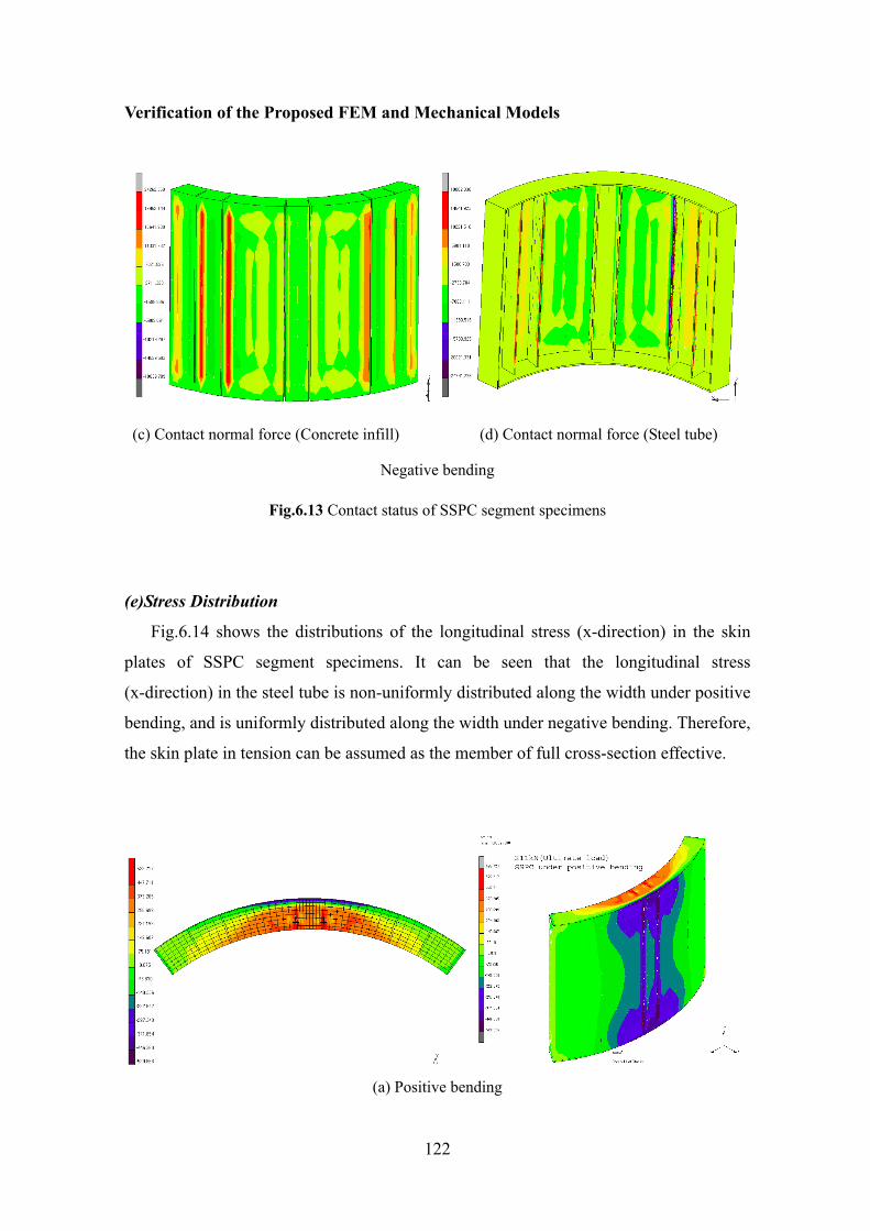
Verification of the Proposed FEM and Mechanical Models
122
(c) Contact normal force (Concrete infill) (d) Contact normal force (Steel tube)
Negative bending
Fig.6.13 Contact status of SSPC segment specimens
(e)Stress Distribution
Fig.6.14 shows the distributions of the longitudinal stress (x-direction) in the skin
plates of SSPC segment specimens. It can be seen that the longitudinal stress
(x-direction) in the steel tube is non-uniformly distributed along the width under positive
bending, and is uniformly distributed along the width under negative bending. Therefore,
the skin plate in tension can be assumed as the member of full cross-section effective.
(a) Positive bending
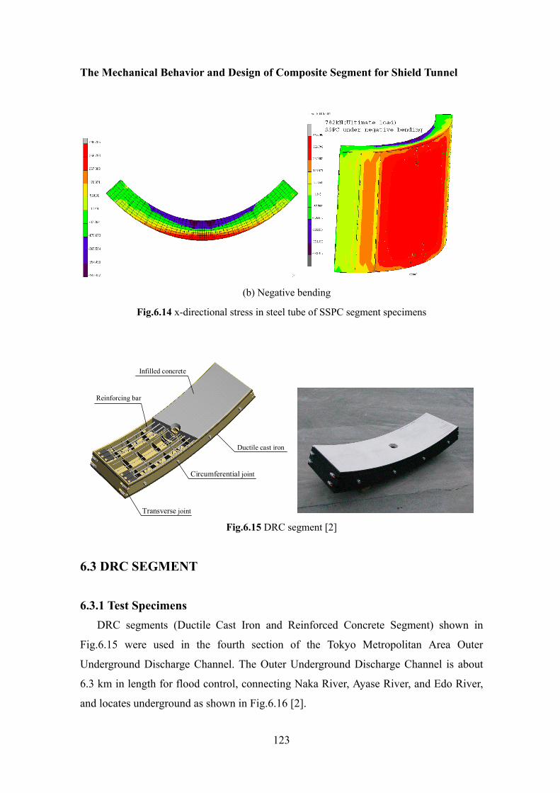
The Mechanical Behavior and Design of Composite Segment for Shield Tunnel
123
(b) Negative bending
Fig.6.14 x-directional stress in steel tube of SSPC segment specimens
Transverse joint
Circumferential joint
Ductile cast iron
Infilled concrete
Reinforcing bar
Fig.6.15 DRC segment [2]
6.3 DRC SEGMENT
6.3.1 Test Specimens DRC segments (Ductile Cast Iron and Reinforced Concrete Segment) shown in
Fig.6.15 were used in the fourth section of the Tokyo Metropolitan Area Outer
Underground Discharge Channel. The Outer Underground Discharge Channel is about
6.3 km in length for flood control, connecting Naka River, Ayase River, and Edo River,
and locates underground as shown in Fig.6.16 [2].
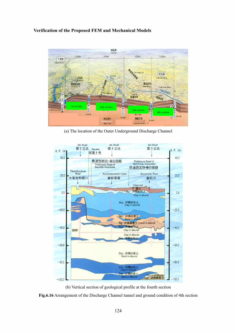
Verification of the Proposed FEM and Mechanical Models
124
1st section 2nd section3rd section
4th section
(a) The location of the Outer Underground Discharge Channel
(b) Vertical section of geological profile at the fourth section
Fig.6.16 Arrangement of the Discharge Channel tunnel and ground condition of 4th section
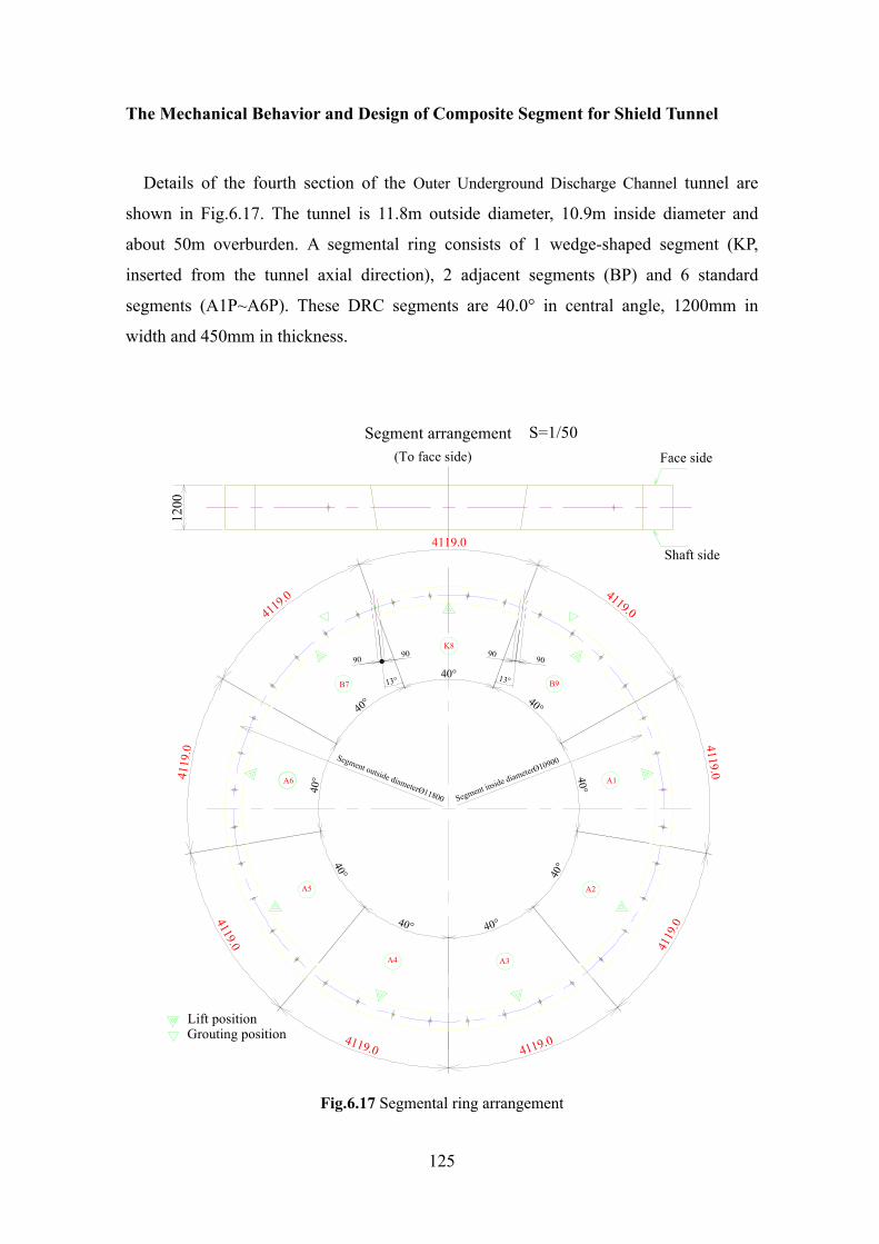
The Mechanical Behavior and Design of Composite Segment for Shield Tunnel
125
Details of the fourth section of the Outer Underground Discharge Channel tunnel are
shown in Fig.6.17. The tunnel is 11.8m outside diameter, 10.9m inside diameter and
about 50m overburden. A segmental ring consists of 1 wedge-shaped segment (KP,
inserted from the tunnel axial direction), 2 adjacent segments (BP) and 6 standard
segments (A1P~A6P). These DRC segments are 40.0° in central angle, 1200mm in
width and 450mm in thickness.
Segment arrangement S=1/50(To face side) Face side
Shaft side
Lift positionGrouting position
A6
B7
K8
B9
A1
A2
A3A4
A5
Fig.6.17 Segmental ring arrangement

Verification of the Proposed FEM and Mechanical Models
126
Details of the standard segments (A1P~A6P) are shown in Fig.6.18. The standard
segments (A1P~A6P) consist of 11mm thickness skin plate, 20mm thickness main
girders(including outside main girders and inside main girders), and 20mm thickness
joint plates of ductile cast iron, and reinforced concrete infilling(reinforcing bars
including D29 main reinforcements and D13 structural reinforcements).
C
C
A
AFace side
Shaft side
SM490
A1~A6 segments S=1/50
B
B
face side shaft sideView C-C S=1/10
face side shaft sideView A-A S=1/10
face side shaft sideView A-A S=1/10
Fig.6.18 Configuration and reinforcing bar layout of A1P~A6P segments

The Mechanical Behavior and Design of Composite Segment for Shield Tunnel
127
In general, the lining member of tunnel is subjected to combined bending, axial and
shear forces. Therefore, it is important to study the mechanical behavior of segments
(called as tunnel lining) under confined bending and axial forces. However, it is very
difficult that the axial force is applied on the segment with curvature in the laboratory
experiments. If the ratio of the thickness of segment to the radius of the tunnel is smaller
than 1/20, the segment without curvature can be used to study the mechanical behavior
of the segment under combined bending and axial forces. In this study, the DRC segment
specimens without curvature of the same dimensions as the actual used DRC segments
in the fourth section of the Outer Underground Discharge Channel tunnel were design
and tested. Details of the standard segment specimens (AP) are shown in Fig.6.19 and
the dimensions of DRC segments are summarized in Table6.4. Mechanical properties of
ductile cast iron, reinforcing bar, and concrete are shown in Table6.5.
400
100
1200
100
350
465
125100 125
365
150 125125100 100
400400
D29 (SD295)150
20
10
100
125
125
100
150
400
100
125
125
100
150
1200
540 475 475 410 540475475410
465
3800
540 475 410475 410 475 475 540
A A
View A-A
B
B
View B-B
Main reinforcements(D29) structural reinforcements(D13)
Inside main girder
Unit: mm
Fig.6.19. Configuration and reinforcing bar layout of DRC segment specimens
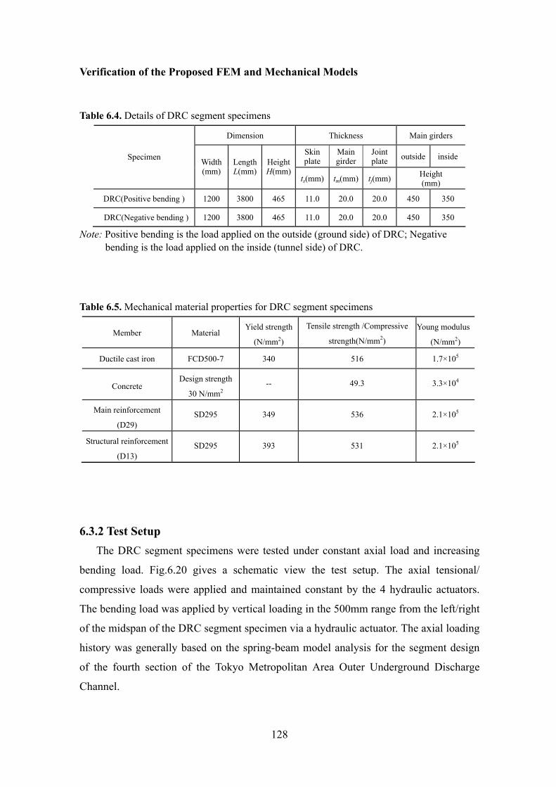
Verification of the Proposed FEM and Mechanical Models
128
Table 6.4. Details of DRC segment specimens
Dimension Thickness Main girders
Skin plate
Main girder
Joint plate outside inside Specimen Width
(mm) LengthL(mm)
HeightH(mm)
ts(mm) tm(mm) tj(mm) Height (mm)
DRC(Positive bending ) 1200 3800 465 11.0 20.0 20.0 450 350
DRC(Negative bending ) 1200 3800 465 11.0 20.0 20.0 450 350
Note: Positive bending is the load applied on the outside (ground side) of DRC; Negative bending is the load applied on the inside (tunnel side) of DRC.
Table 6.5. Mechanical material properties for DRC segment specimens
Member Material Yield strength
(N/mm2)
Tensile strength /Compressive
strength(N/mm2)
Young modulus
(N/mm2)
Ductile cast iron FCD500-7 340 516 1.7×10⁵
Concrete Design strength
30 N/mm2 -- 49.3 3.3×10⁴
Main reinforcement
(D29) SD295 349 536 2.1×10⁵
Structural reinforcement
(D13) SD295 393 531 2.1×10⁵
6.3.2 Test Setup The DRC segment specimens were tested under constant axial load and increasing
bending load. Fig.6.20 gives a schematic view the test setup. The axial tensional/
compressive loads were applied and maintained constant by the 4 hydraulic actuators.
The bending load was applied by vertical loading in the 500mm range from the left/right
of the midspan of the DRC segment specimen via a hydraulic actuator. The axial loading
history was generally based on the spring-beam model analysis for the segment design
of the fourth section of the Tokyo Metropolitan Area Outer Underground Discharge
Channel.
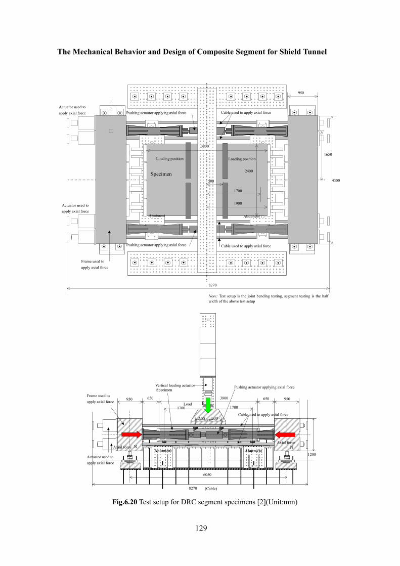
The Mechanical Behavior and Design of Composite Segment for Shield Tunnel
129
4300
Note: Test setup is the joint bending testing, segment testing is the half width of the above test setup
1650
8270
500
1700
1900
950
2400
3800
Abutment
Specimen
Loading position
Cable used to apply axial force
Pushing actuator applying axial force
Frame used to apply axial force
Actuator used to apply axial force
Actuator used to apply axial force Pushing actuator applying axial force Cable used to apply axial force
Abutment
Loading position
Fig.6.20 Test setup for DRC segment specimens [2](Unit:mm)
(Cable)8270
1200
6050
1700 1700
500 500
3800
950 650
950 650
Vertical loading actuator
Frame used to apply axial force
Actuator used to apply axial force
Abutment
Pushing actuator applying axial force
Specimen
Cable used to apply axial force Load P
Axial force N N Abutment
Axial force

Verification of the Proposed FEM and Mechanical Models
130
The testing steps of DRC segment specimens under combined positive bending/
negative bending and axial load are shown in Fig.6.21, and consist of the 4 test steps.
The first three steps are the applied load reached the yield carrying capacity under
compressive axial load, no axial load, and tensional axial load respectively. The last step
is the applied load reached the DRC segment specimens failure under no axial load.
Displacement transducers and Strain gauges located on the key points shown in Fig.6.22
and Fig.6.23 were used to measure strains and deflections, respectively.
Case1No inner water pressure
Case2Inner water pressure
N=0kN(positive)N=0kN(negative)
N=345kN(positive)N=521kN(negative)
Design load(Case2)P=199kN(positive)P=223kN(negative)
Allowable carrying capacityP=1050kN(positive)P=1215kN(negative)
N=0kN(positive)N=0kN(negative)
N=-4767kN(positive)N=-5283kN(negative)
Full plastic LoadP=3645kN(positive)P=4145kN(negative)
Yield LoadP=1757kN(positive)P=2839kN(negative)
Allowable carrying capacityP=1050kN(positive)P=1215kN(negative)
allowable carrying capacityP=997kN(positive)P=720kN(negative)
Actual allowable carrying capacityP=1499kN(positive)P=2442kN(negative)
Design load(Case1)P=672kN(positive)P=471kN(negative)
Ver
tical
load
ing(
bend
ing
load
)
Axial load
Fig.6.21 Testing steps
The numbers 1,2,3 etc. denote the serial numbers of displacement transducer :displacement transducer Unit : mm
1
3
26 4
200 3800
8
7
500 9
5
200450500450
1200
1011
12
14
13
15
600
Fig. 6.22 The arrangement of displacement transducers on DRC segment specimens

The Mechanical Behavior and Design of Composite Segment for Shield Tunnel
131
475 475 475 475450 400 100 500 450
200 200
600
600
125
125
100
150
150
100
125
125
Mian measuring section
Abutment Abutment
Loading position Loading position
WFLA-6-11-5LT
FLA-5-11-5LT
WFLA-6-11-5LT
FLA-5-11-5LT
WFLA-6-11-5LT
FLA-5-11-5LTFLA-5-11-5LT
FLA-5-11-5LT WFLA-6-11-5LT with waterproof
Strain fixed only the outsidefor main girder
(a) The arrangement of strain gauges on skin plate
125
125
100
150
125
125
100
150
1200
475 475 475 475450 400100
500 450
200 200
Mian measuring section
Abutment Abutment
Loading position Loading position
465
100
100
100
200 200Abutment Abutment10
010
010
010
0200
200
Longtitudinal direction(WFLA-6-11-5LT ;FLA-5-11-5LT )
Transversal direction(WFLA-6-11-5LT ;FLA-5-11-5LT )
Outside main girder
Inside main girder
(b) The arrangement of strain gauges on main girders
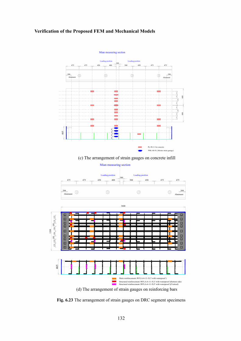
Verification of the Proposed FEM and Mechanical Models
132
475 475 475 475450 400100
500 450
200 200
600
600
125
125
100
150
150
100
125
125
Mian measuring section
Abutment Abutment
Loading position Loading position
PML-60-5L (Mortar strain gauage)
PL-90-11 for concrete
465
100
100
100
100
(c) The arrangement of strain gauges on concrete infill
125
125
100
150
125
125
100
150
1200
3800
475 475 475 475450 400100
500 450
200 200
Mian measuring section
Abutment Abutment
Loading position Loading position
465
Main reinforcement (WFLA-6-11-5LT with waterproof )Structural reinforcement (WFLA-6-11-5LT with waterproof )(bottom side)Structural reinforcement (WFLA-6-11-5LT with waterproof )(Vertical)
(d) The arrangement of strain gauges on reinforcing bars
Fig. 6.23 The arrangement of strain gauges on DRC segment specimens
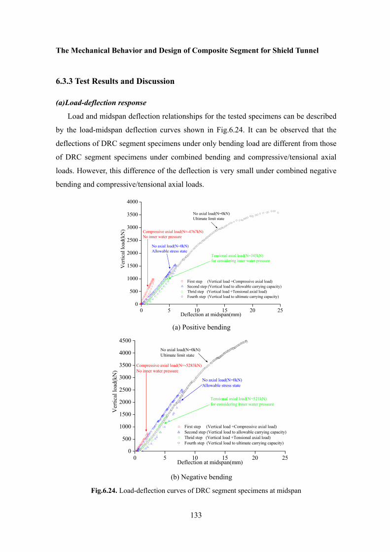
The Mechanical Behavior and Design of Composite Segment for Shield Tunnel
133
6.3.3 Test Results and Discussion (a)Load-deflection response
Load and midspan deflection relationships for the tested specimens can be described
by the load-midspan deflection curves shown in Fig.6.24. It can be observed that the
deflections of DRC segment specimens under only bending load are different from those
of DRC segment specimens under combined bending and compressive/tensional axial
loads. However, this difference of the deflection is very small under combined negative
bending and compressive/tensional axial loads.
0 5 10 15 20 250
500
1000
1500
2000
2500
3000
3500
4000
Tensional axial load(N=345kN)for considering inner water pressure
No axial load(N=0kN)Allowable stress state
No axial load(N=0kN)Ultimate limit state
Compressive axial load(N=-4767kN)No inner water pressure
Ver
tical
load
(kN
)
Deflection at midspan(mm)
First step (Vertical load +Compressive axial load) Second step (Vertical load to allowable carrying capacity)Thrid step (Vertical load +Tensional axial load) Fourth step (Vertical load to ultimate carrying capacity)
(a) Positive bending
0 5 10 15 20 250
500
1000
1500
2000
2500
3000
3500
4000
4500
Tensional axial load(N=521kN)for considering inner water pressure
No axial load(N=0kN)Allowable stress state
No axial load(N=0kN)Ultimate limit state
Compressive axial load(N=-5283kN)No inner water pressure
Ver
tical
load
(kN
)
Deflection at midspan(mm)
First step (Vertical load +Compressive axial load) Second step (Vertical load to allowable carrying capacity)Thrid step (Vertical load +Tensional axial load) Fourth step (Vertical load to ultimate carrying capacity)
(b) Negative bending
Fig.6.24. Load-deflection curves of DRC segment specimens at midspan
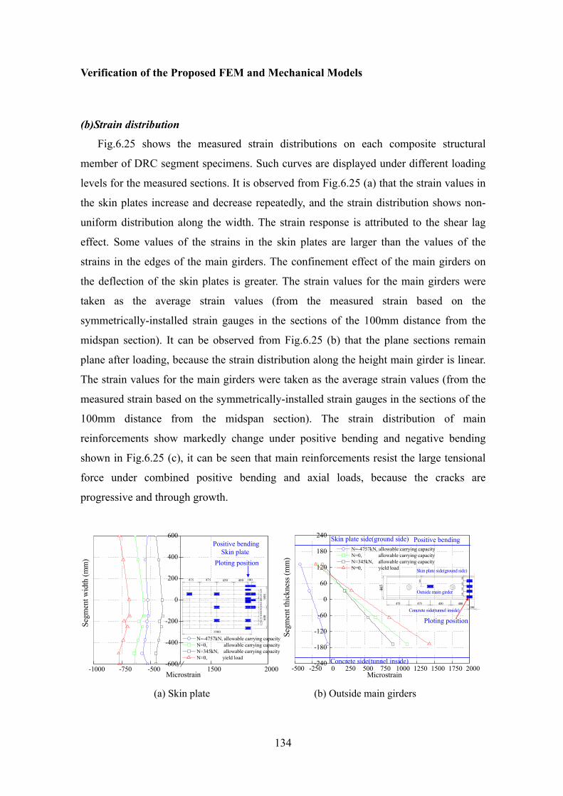
Verification of the Proposed FEM and Mechanical Models
134
(b)Strain distribution
Fig.6.25 shows the measured strain distributions on each composite structural
member of DRC segment specimens. Such curves are displayed under different loading
levels for the measured sections. It is observed from Fig.6.25 (a) that the strain values in
the skin plates increase and decrease repeatedly, and the strain distribution shows non-
uniform distribution along the width. The strain response is attributed to the shear lag
effect. Some values of the strains in the skin plates are larger than the values of the
strains in the edges of the main girders. The confinement effect of the main girders on
the deflection of the skin plates is greater. The strain values for the main girders were
taken as the average strain values (from the measured strain based on the
symmetrically-installed strain gauges in the sections of the 100mm distance from the
midspan section). It can be observed from Fig.6.25 (b) that the plane sections remain
plane after loading, because the strain distribution along the height main girder is linear.
The strain values for the main girders were taken as the average strain values (from the
measured strain based on the symmetrically-installed strain gauges in the sections of the
100mm distance from the midspan section). The strain distribution of main
reinforcements show markedly change under positive bending and negative bending
shown in Fig.6.25 (c), it can be seen that main reinforcements resist the large tensional
force under combined positive bending and axial loads, because the cracks are
progressive and through growth.
-1000 -750 -500 1500 2000-600
-400
-200
0
200
400
600Positive bending
475 475 450 400 100
600
600
1251
2510
0150
1501
0012
512
5
1900
Skin platePloting position
Microstrain
Segm
ent w
idth
(mm
)
N=-4757kN, allowable carrying capacity N=0, allowable carrying capacity N=345kN, allowable carrying capacity N=0, yield load
-500 -250 0 250 500 750 1000 1250 1500 1750 2000-240
-180
-120
-60
0
60
120
180
240Positive bending
Concrete side(tunnel inside)
100
100
100
100
200
465
475 475 450 400100
Outside main girder
Skin plate side(ground side)
Concrete side(tunnel inside)
Skin plate side(ground side)
Ploting position
Microstrain
Segm
ent t
hick
ness
(mm
)
N=-4757kN, allowable carrying capacity N=0, allowable carrying capacity N=345kN, allowable carrying capacity N=0, yield load
(a) Skin plate (b) Outside main girders

The Mechanical Behavior and Design of Composite Segment for Shield Tunnel
135
-2000 -1600 -1200 -800 -400 0 400 800 1200 1600 2000-600
-400
-200
0
200
400
600
Positive bending
125
1251
0015
012
512
510
015
0
1200
1900
475 475 450 400 100
Main reinforcement
Ploting position
Microstrain
Segm
ent w
idth
(mm
)
N=-
4757
kN, a
llow
able
car
ryin
g ca
paci
ty N
=0,
a
llow
able
car
ryin
g ca
paci
ty N
=345
kN,
allo
wab
le c
arry
ing
capa
city
N=0
,
yie
ld lo
ad-200 -150 -100 -50 0 50 100 150
-600
-400
-200
0
200
400
600
465
100
100
225
365
225
365
1200
475 475 450 400 100CL
Positive bendingCentral rib
Ploting position
Microstrain
Segm
ent w
idth
(mm
)
N=-4757kN, allowable carrying capacity N=0, allowable carrying capacity N=345kN, allowable carrying capacity N=0, yield load
(c) Main reinforcements (d) Central rib Positive bending
-3500-3000-2500-2000-1500-1000 -500 0 500 1000 1500 2000-600
-400
-200
0
200
400
600Negative bending
475 475 450 400 100
600
600
1251
2510
0150
1501
0012
512
5
1900
Skin platePloting position
Microstrain
Segm
ent w
idth
(mm
)
N=-5283kN, allowable carrying capacity N=0, allowable carrying capacity N=521kN, allowable carrying capacity N=0, yield load
-1500 -1000 -500 0 500 1000 1500 2000-240
-180
-120
-60
0
60
120
180
240
Negative bendingSkin plate side(ground side)
Concrete side(tunnel inside)
100
1001
0010
020046
5
475 475 450 400 100
Outside main girder
N=-5283kN, allowable carrying capacity N=0, allowable carrying capacity N=521kN, allowable carrying capacity N=0, yield load
Concrete side(tunnel inside)
Skin plate side(ground side)
Ploting position
Microstrain
Segm
ent t
hick
ness
(mm
)
(a) Skin plate (b) Outside main girders
-600 -400 -200 0 200 400 600 800 1000-600
-400
-200
0
200
400
600
N=-5283kN, allowable carrying capacity N=0, allowable carrying capacity N=521kN, allowable carrying capacity N=0, yield load
Negative bending
1251
2510
0 150
125
125
100
150
1200
1900
475 475 450 400 100
Main reinforcement
Ploting position
Microstrain
Segm
ent w
idth
(mm
)
-150 -100 -50 0 50 100 150 200-600
-400
-200
0
200
400
600
N=-5283kN, allowable carrying capacity N=0, allowable carrying capacity N=521kN, allowable carrying capacity N=0, yield load
465
100
100
225
365
225
365
1200
475 475 450 400 100CL
Negative bendingCentral rib
Ploting position
Microstrain
Segm
ent w
idth
(mm
)
(c) Main reinforcements (d) Central rib
Negative bending
Fig.6.25. Measured strain distribution
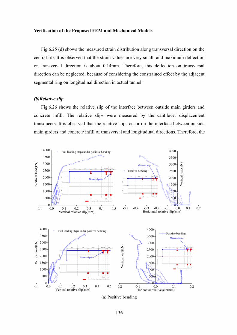
Verification of the Proposed FEM and Mechanical Models
136
Fig.6.25 (d) shows the measured strain distribution along transversal direction on the
central rib. It is observed that the strain values are very small, and maximum deflection
on transversal direction is about 0.14mm. Therefore, this deflection on transversal
direction can be neglected, because of considering the constrained effect by the adjacent
segmental ring on longitudinal direction in actual tunnel.
(b)Relative slip
Fig.6.26 shows the relative slip of the interface between outside main girders and
concrete infill. The relative slips were measured by the cantilever displacement
transducers. It is observed that the relative slips occur on the interface between outside
main girders and concrete infill of transversal and longitudinal directions. Therefore, the
-0.1 0.0 0.1 0.2 0.3 0.4 0.50
500
1000
1500
2000
2500
3000
3500
4000
600
4 7 5 4 7 5 4 5 0 4 @ 1 0 0 1 0 0
465
C an tile v e r d isp lacem e n t tran sd ucers
L 4 L 2 a L 1 a
Measured point
Ver
tical
load
(kN
)
Vertical relative slip(mm)
Full loading steps under positive bending
-0.5 -0.4 -0.3 -0.2 -0.1 0.0 0.1 0.2
0
500
1000
1500
2000
2500
3000
3500
4000
600
4 7 5 4 7 5 4 5 0 4 @ 1 0 0 1 0 0
465
C an tile v e r d isp la ce m e n t tran sd u ce rs
L 4 L 2 a L 1 a
Measured point
Ver
tical
load
(kN
)
Horizontal relative slip(mm)
Positive bending
-0.1 0.0 0.1 0.2 0.3 0.4 0.50
500
1000
1500
2000
2500
3000
3500
4000
600
4 7 5 4 7 5 4 5 0 4 @ 1 0 0 1 0 0
465
C an tile v e r d isp lacem e n t tran sd u ce rs
L 4 L 2 a L 1 a
Measured point
Ver
tical
load
(kN
)
Vertical relative slip(mm)
Full loading steps under positive bending
-0.2 -0.1 0.0 0.1 0.2
0
500
1000
1500
2000
2500
3000
3500
4000
600
4 7 5 4 7 5 4 5 0 4 @ 1 0 0 1 0 0
465
C a n tile v e r d isp la ce m e n t tra n sd u ce rs
L 4 L 2 a L 1 a
Measured point
Ver
tical
load
(kN
)
Horizontal relative slip(mm)
Positive bending
(a) Positive bending
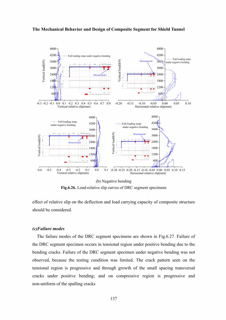
The Mechanical Behavior and Design of Composite Segment for Shield Tunnel
137
-0.3 -0.2 -0.1 0.0 0.1 0.2 0.3 0.4 0.5 0.6 0.7 0.80
600
1200
1800
2400
3000
3600
4200
4800
600
4 7 5 4 7 5 4 5 0 4@ 1 0 0 10 0
465
C an tile v e r d isp lacem e n t tran sd u cers
L 4 L 2 a L 1 a
Measured point
Ver
tical
load
(kN
)
Vertical relative slip(mm)
Full loading steps under negative bending
-0.20 -0.15 -0.10 -0.05 0.00 0.05 0.10
0
600
1200
1800
2400
3000
3600
4200
4800
Ver
tical
load
(kN
)60
0
4 75 47 5 4 5 0 4 @ 1 00 1 0 0
465
C an tilev e r d isp lacem en t tran sdu cers
L 4 L 2a L 1 a
Measured point
Horizontal relative slip(mm)
Full loading steps under negative bending
-0.6 -0.5 -0.4 -0.3 -0.2 -0.1 0.0 0.10
600
1200
1800
2400
3000
3600
4200
4800
Ver
tical
load
(kN
)60
0
4 7 5 4 7 5 4 5 0 4 @ 1 0 0 1 0 0
465
C an tile v e r d isp lacem e n t tran sd u ce rs
L 4 L 2 a L 1 a
Measured point
Vertical relative slip(mm)
Full loading steps under negative bending
-0.30 -0.25 -0.20 -0.15 -0.10 -0.05 0.00 0.05 0.10 0.15
0
600
1200
1800
2400
3000
3600
4200
4800V
ertic
al lo
ad(k
N)
600
4 7 5 4 7 5 4 5 0 4 @ 1 0 0 1 0 0
465
C a n tile v e r d isp la ce m e n t tra n sd u ce rs
L 4 L 2 a L 1 a
Measured point
Horizontal relative slip(mm)
Full loading steps under negative bending
(b) Negative bending
Fig.6.26. Load-relative slip curves of DRC segment specimens
effect of relative slip on the deflection and load carrying capacity of composite structure
should be considered.
(c)Failure modes
The failure modes of the DRC segment specimens are shown in Fig.6.27. Failure of
the DRC segment specimen occurs in tensional region under positive bending due to the
bending cracks. Failure of the DRC segment specimen under negative bending was not
observed, because the testing condition was limited. The crack pattern seen on the
tensional region is progressive and through growth of the small spacing transversal
cracks under positive bending; and on compressive region is progressive and
non-uniform of the spalling cracks

Verification of the Proposed FEM and Mechanical Models
138
Width of the cracks(Unit: mm): ①0.08,②0.15,③0.10,④0.08,⑤0.10,⑥0.06,⑦0.06,⑧less than0.04,⑨less than 0.04,⑩0.04
①② ③④⑤⑥
⑦⑧ ⑨
(a) The cracks distribution of third loading step
(b) The cracks distribution at failure
Fig.6.27. Failure modes under combined positive bending and axial loads [2]
6.3.4 FEM Results and Discussion Only one quarter of each the DRC segment specimens are modeled taking advantage
of symmetry in two mutually perpendicular vertical planes shown in Fig6.28. Symmetric
boundary conditions are applied at the two vertical planes of symmetry. 8-Node 3D solid
elements with tri-linear interpolation and nonlinear interpolation are used to model steel
plates and concrete, respectively. 8-Node 3D solid element with bi-linear interpolation is
used to model reinforcing bars. The vertical and horizontal constraints are applied at the
bottom of the support along its centre line and mid-span section respectively.
Longitudinal load is distributed to all the nodes on top of the loading plate, with nodes at
symmetry plane getting half of the load at rest of the nodes. Axial load is given as a
uniform pressure load at the DRC segment end. It is applied in first and third loading
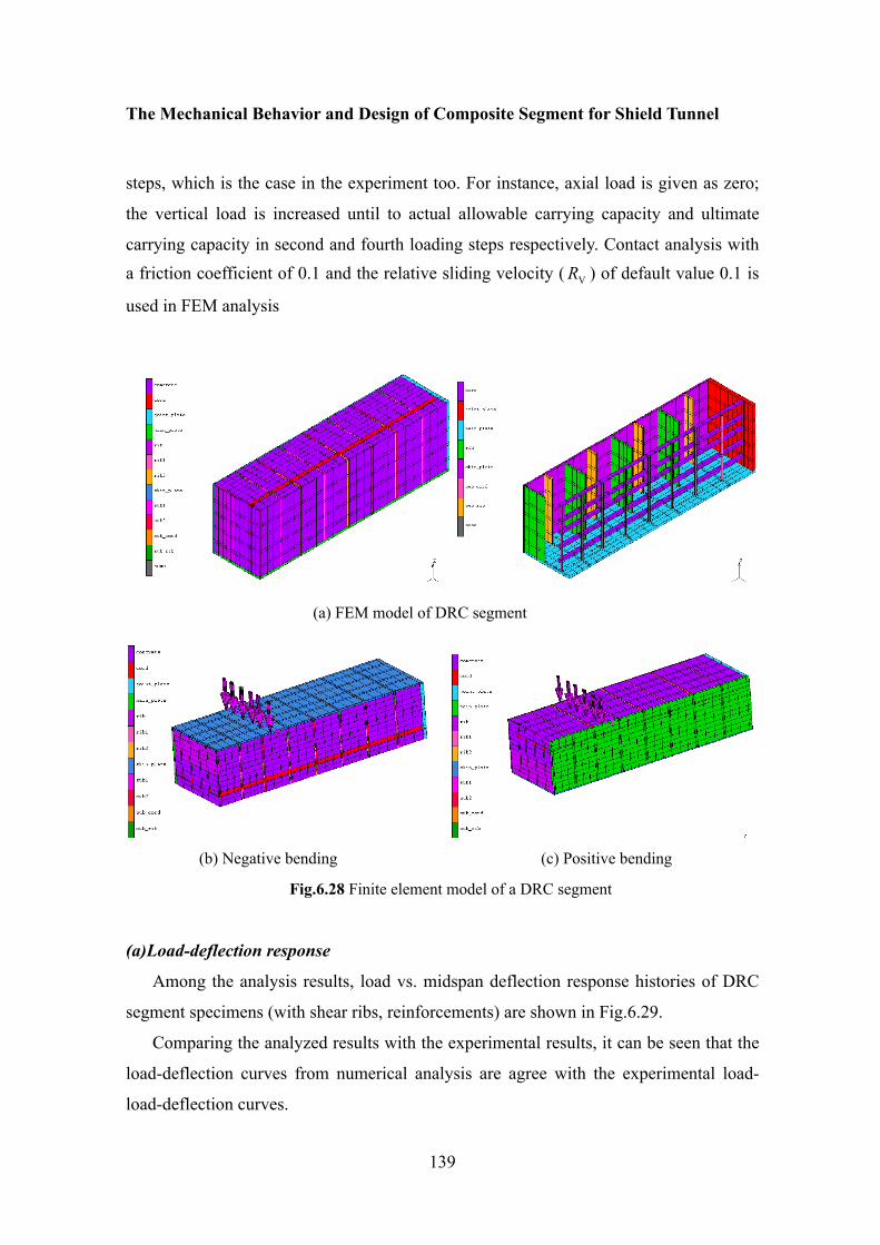
The Mechanical Behavior and Design of Composite Segment for Shield Tunnel
139
steps, which is the case in the experiment too. For instance, axial load is given as zero;
the vertical load is increased until to actual allowable carrying capacity and ultimate
carrying capacity in second and fourth loading steps respectively. Contact analysis with a friction coefficient of 0.1 and the relative sliding velocity ( VR ) of default value 0.1 is
used in FEM analysis
(a) FEM model of DRC segment
(b) Negative bending (c) Positive bending
Fig.6.28 Finite element model of a DRC segment
(a)Load-deflection response
Among the analysis results, load vs. midspan deflection response histories of DRC
segment specimens (with shear ribs, reinforcements) are shown in Fig.6.29.
Comparing the analyzed results with the experimental results, it can be seen that the
load-deflection curves from numerical analysis are agree with the experimental load-
load-deflection curves.
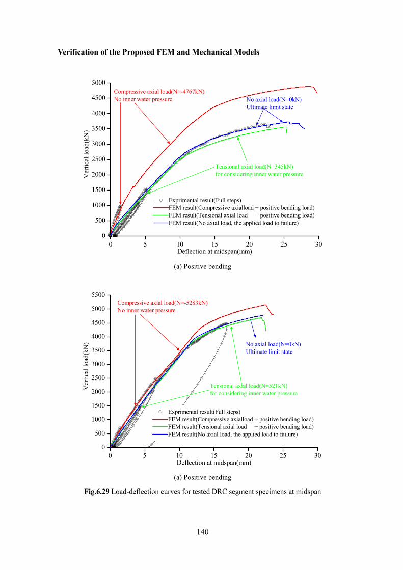
Verification of the Proposed FEM and Mechanical Models
140
0 5 10 15 20 25 300
500
1000
1500
2000
2500
3000
3500
4000
4500
5000
Tensional axial load(N=345kN)for considering inner water pressure
No axial load(N=0kN)Ultimate limit state
Compressive axial load(N=-4767kN)No inner water pressure
Ver
tical
load
(kN
)
Deflection at midspan(mm)
Exprimental result(Full steps)FEM result(Compressive axialload + positive bending load)FEM result(Tensional axial load + positive bending load) FEM result(No axial load, the applied load to failure)
(a) Positive bending
0 5 10 15 20 25 300
500
1000
1500
2000
2500
3000
3500
4000
4500
5000
5500
Tensional axial load(N=521kN)for considering inner water pressure
Compressive axial load(N=-5283kN)No inner water pressure
No axial load(N=0kN)Ultimate limit state
Ver
tical
load
(kN
)
Deflection at midspan(mm)
Exprimental result(Full steps)FEM result(Compressive axialload + positive bending load)FEM result(Tensional axial load + positive bending load) FEM result(No axial load, the applied load to failure)
(a) Positive bending
Fig.6.29 Load-deflection curves for tested DRC segment specimens at midspan
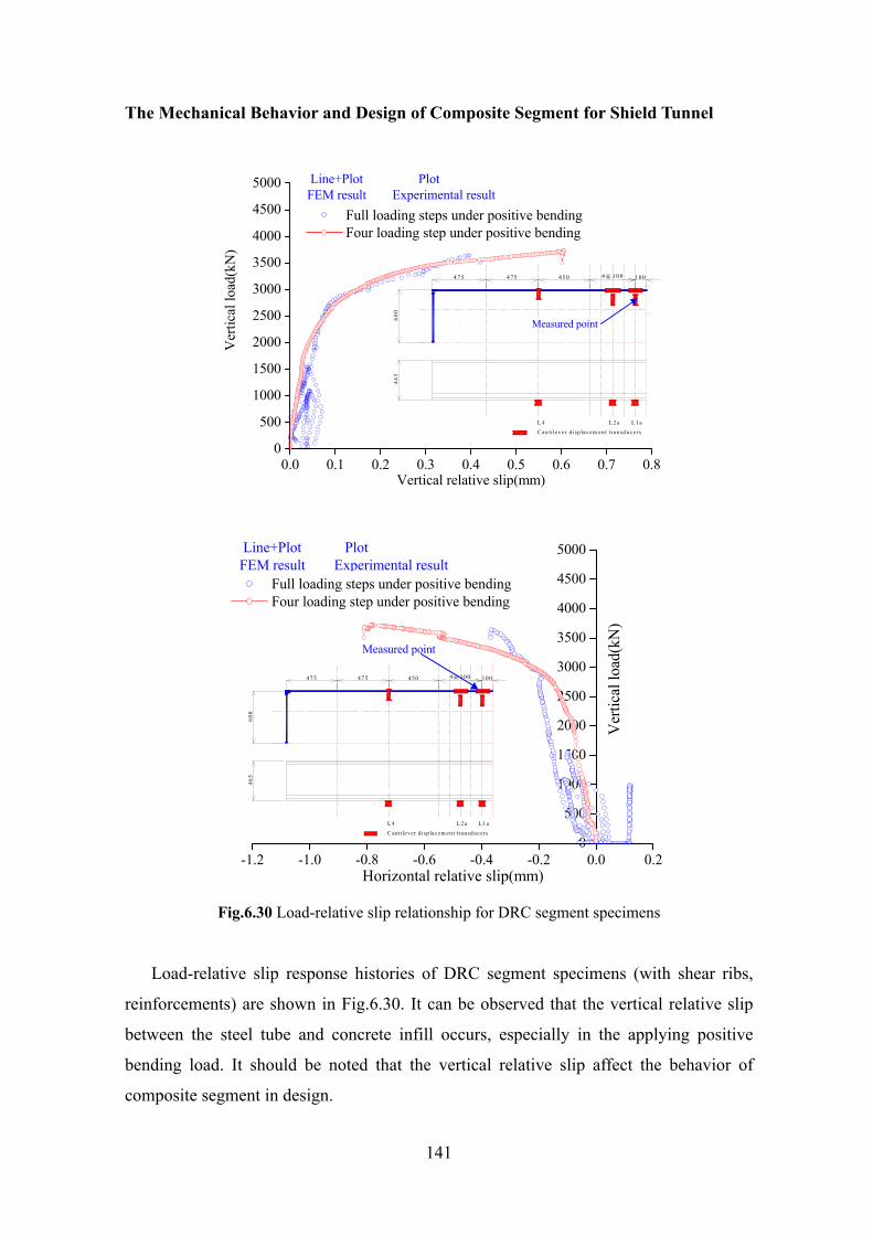
The Mechanical Behavior and Design of Composite Segment for Shield Tunnel
141
0.0 0.1 0.2 0.3 0.4 0.5 0.6 0.7 0.80
500
1000
1500
2000
2500
3000
3500
4000
4500
5000 Line+Plot PlotFEM result Experimental result
600
4 7 5 4 7 5 4 5 0 4 @ 1 0 0 1 0 0
465
C an tile v er d isp lacem e n t tran sd u cers
L 4 L 2 a L 1 a
Measured point
Ver
tical
load
(kN
)
Vertical relative slip(mm)
Full loading steps under positive bending Four loading step under positive bending
-1.2 -1.0 -0.8 -0.6 -0.4 -0.2 0.0 0.20
500
1000
1500
2000
2500
3000
3500
4000
4500
5000 Line+Plot PlotFEM result Experimental result
Full loading steps under positive bending Four loading step under positive bending
600
47 5 47 5 450 4@ 100 100
465
C antilever d isp lacem en t transd ucers
L 4 L 2a L 1a
Measured point
Ver
tical
load
(kN
)
Horizontal relative slip(mm) Fig.6.30 Load-relative slip relationship for DRC segment specimens
Load-relative slip response histories of DRC segment specimens (with shear ribs,
reinforcements) are shown in Fig.6.30. It can be observed that the vertical relative slip
between the steel tube and concrete infill occurs, especially in the applying positive
bending load. It should be noted that the vertical relative slip affect the behavior of
composite segment in design.

Verification of the Proposed FEM and Mechanical Models
142
(b)Strain distribution Fig.6.31 shows the strain distributions at the measured locations. The strain
distributions of nonlinear analysis show good agreement with the experimental results in
main girders. The tendency of the strain distribution of nonlinear analysis shows close
agreement with the experimental value in the skin plates. In addition, the strain
distribution along the skin plate width for DRC segment specimens is uniform. It can be
concluded that the evaluation of shear studs is necessary to design composite segments.
-1000 -800 -600 -400 0 200 400 600 800
-600
-300
0
300
600Positive bending
Line PlotFEM result Experimental result
475 475 450 400 100
600
600
1251
2510
0150
1501
0012
512
5
1900
Skin platePloting position
Microstrain
Segm
ent w
idth
(mm
)
N=-4757kN, allowable carrying capacity N=0, allowable carrying capacity N=345kN, allowable carrying capacity N=0, yield load
-3500-3000-2500-2000-1500-1000 -500 0 500 1000 1500 2000-600
-400
-200
0
200
400
600
Line PlotFEM result Experimental result
Negative bending
475 475 450 400 100
600
600
1251
2510
0150
1501
0012
512
5
1900
Skin platePloting position
Microstrain
Segm
ent w
idth
(mm
)
N=-5283kN, allowable carrying capacity N=0, allowable carrying capacity N=521kN, allowable carrying capacity N=0, yield load
(a) Strain distribution for skin plate
-1200-900 -600 -300 0 300 600 900 12001500180021002400-300
-240
-180
-120
-60
0
60
120
180
240 Line Plot Positive bendingFEM result Experimental result
N=-4757kN, allowable carrying capacity N=0, allowable carrying capacity N=345kN, allowable carrying capacity N=0, yield load
Concrete side(tunnel inside)
100
100
100
100
200
465
475 475 450 400100
Outside main girder
Skin plate side(ground side)
Concrete side(tunnel inside)
Skin plate side(ground side)
Ploting position
Microstrain
Segm
ent t
hick
ness
(mm
)
-1500 -1000 -500 0 500 1000 1500
-240
-180
-120
-60
0
60
120
180
240
300 Line PlotFEM result Experimental result
Negative bendingSkin plate side(ground side)
Concrete side(tunnel inside)
100
1001
0010
020046
5
475 475 450 400 100
Outside main girder
N=-5283kN, allowable carrying capacity N=0, allowable carrying capacity N=521kN, allowable carrying capacity N=0, yield load
Concrete side(tunnel inside)
Skin plate side(ground side)
Ploting position
Microstrain
Segm
ent t
hick
ness
(mm
)
(b) Strain distribution for main girder

The Mechanical Behavior and Design of Composite Segment for Shield Tunnel
143
-800 -400 400 800 1200 1600-600
-400
-200
0
200
400
600 Line PlotFEM result Experimental result
N=-
4757
kN, a
llow
able
car
ryin
g ca
paci
ty N
=0,
a
llow
able
car
ryin
g ca
paci
ty N
=345
kN,
allo
wab
le c
arry
ing
capa
city
N=0
,
yie
ld lo
ad
Positive bending12
512
5100
150
125
125
100
150
1200
1900
475 475 450 400 100
Main reinforcementPloting position
Microstrain
Segm
ent w
idth
(mm
)
- 6 0 0 -4 0 0 -2 0 0 0 2 0 0 4 0 0-6 0 0
-4 0 0
-2 0 0
0
2 0 0
4 0 0
6 0 0
L in e P lo tF E M r e s u l t E x p e r im
N = -5 2 8 3 k N , a N = 0 , a N = 5 2 1 k N , a N = 0 , y
N e g a t iv e b e n d in g
1 9 0 0
4 7 5 4 7 5 4 5
M a in r e in fo rc e m e n tP lo
M ic ro s tr a in
Segm
ent w
idth
(mm
)
(c) Strain distribution for main reinforcements
Fig.6.31 Strain distribution for the members of DRC segment specimens
(c)Failure modes
Fig. 6.32 shows images of the finite element model and the experiments for DRC
segment specimens, with those deformed geometry. It can be seen that the crack pattern
predicted using the finite element model is similar to the observed pattern.
(a) Equivalent of cracking strain in tension
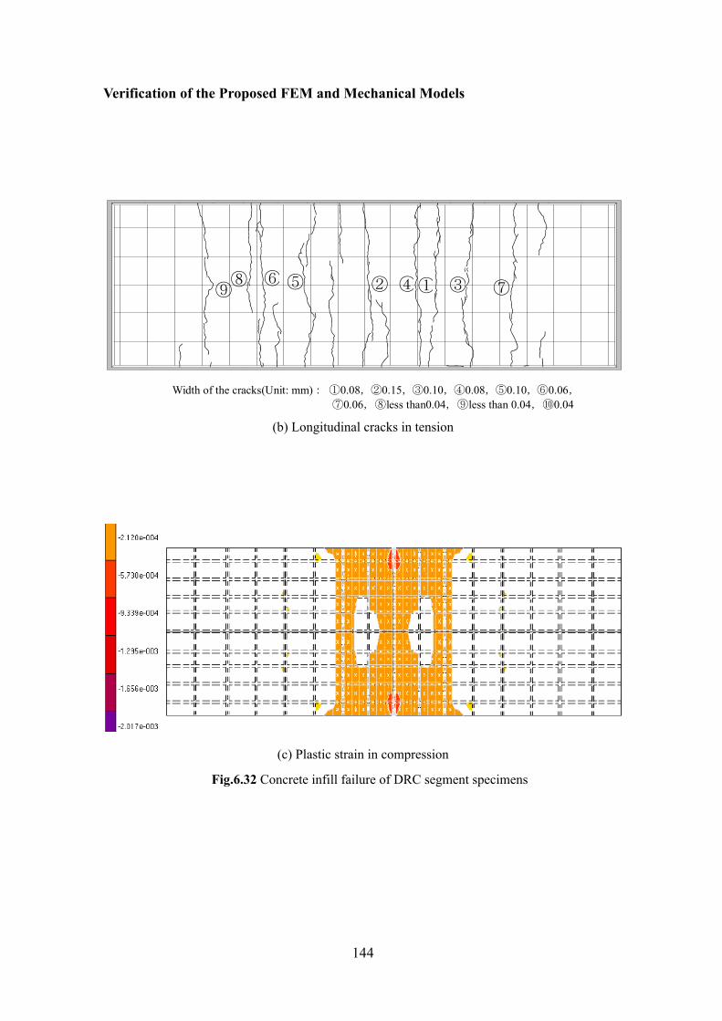
Verification of the Proposed FEM and Mechanical Models
144
Width of the cracks(Unit: mm): ①0.08,②0.15,③0.10,④0.08,⑤0.10,⑥0.06,⑦0.06,⑧less than0.04,⑨less than 0.04,⑩0.04
①② ③④⑤⑥
⑦⑧ ⑨
(b) Longitudinal cracks in tension
(c) Plastic strain in compression
Fig.6.32 Concrete infill failure of DRC segment specimens
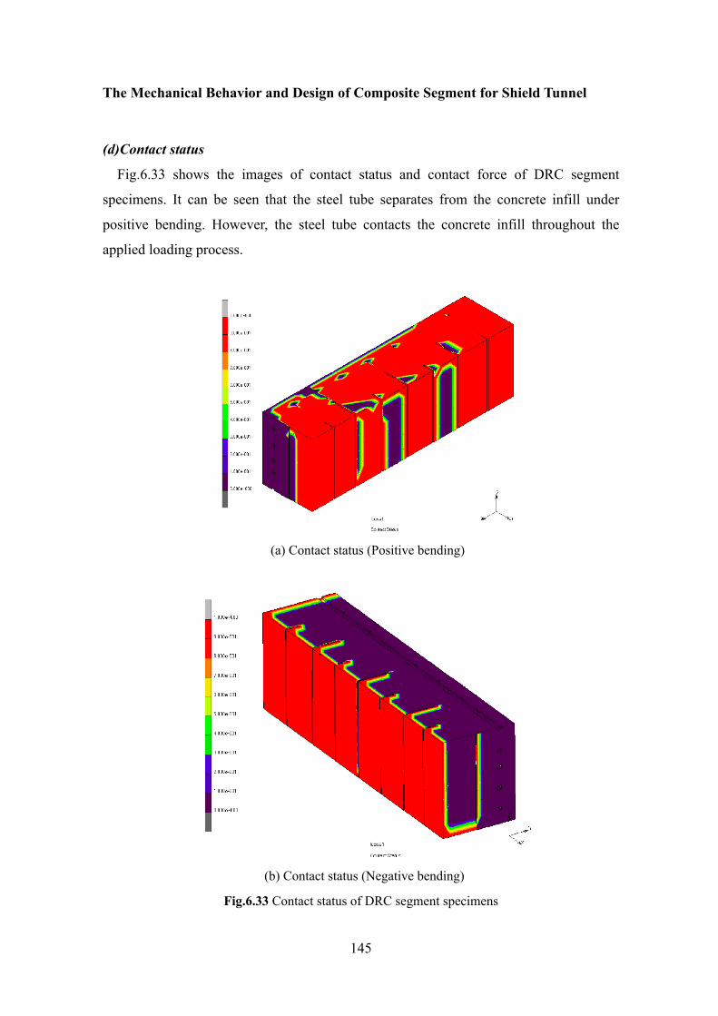
The Mechanical Behavior and Design of Composite Segment for Shield Tunnel
145
(d)Contact status
Fig.6.33 shows the images of contact status and contact force of DRC segment
specimens. It can be seen that the steel tube separates from the concrete infill under
positive bending. However, the steel tube contacts the concrete infill throughout the
applied loading process.
(a) Contact status (Positive bending)
(b) Contact status (Negative bending)
Fig.6.33 Contact status of DRC segment specimens
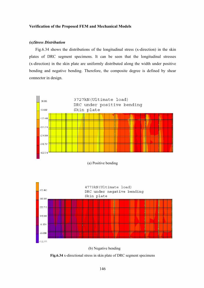
Verification of the Proposed FEM and Mechanical Models
146
(e)Stress Distribution
Fig.6.34 shows the distributions of the longitudinal stress (x-direction) in the skin
plates of DRC segment specimens. It can be seen that the longitudinal stresses
(x-direction) in the skin plate are uniformly distributed along the width under positive
bending and negative bending. Therefore, the composite degree is defined by shear
connector in design.
(a) Positive bending
(b) Negative bending
Fig.6.34 x-directional stress in skin plate of DRC segment specimens

The Mechanical Behavior and Design of Composite Segment for Shield Tunnel
147
6.4 RESULTS AND DISCUSSION OF THE MECHANICAL MODEL
The applicability of the proposed mechanical model based on Closed-composite
segment is verified by comparing the experimental results of SSPC segment and DRC
segment. The following contents should be replaced, when the proposed mechanical
model is used in the structural analysis of others type segment.
(1) 0 Positive bending0 negative bending
bslip
t
γγ
γ=⎧
= ⎨ =⎩, and s-t 0k = / s-b 0k = , because of one skin
plate.
(2) No relative slip occurs between concrete and reinforcement. (3) The post-buckling stress udf ′ is defined by the parameters of the used materials.
(4) Stud shear connector is replaced by rib shear connector. The shear strength of a
rib shear connector is calculated by Eq.(2.26).
Displacement equilibrium can be written as follows: Substituting 0bγ = , 0tγ = into Eqs.(5.24) and (5.25) gives:
1 1t t Vγ α γ η′′ = − + (6.1)
2 2b b Vγ α γ η′′ = − + (6.2)
For the load cases shown in Fig.5.4, solving Eqs. (6.1) and (6.2), and using the boundary conditions that
0 00t bx x
γ γ= == = ,
/ 2 / 20t bx L x L
γ γ= =
′ ′= = and / 2V P= gives
the relative slip solution
( )( )
1
2 1
L x L x
L
P e e e
e
λ λ λ λ
λ
ηγ
− − −
−
+ − −=
+ (6.3)
Correspondingly, the relative slip strain solution is
( )( )2 1
x x L
s L
P e e
e
λ λ λ
λ
ηλε
− −
−
−=
+ (6.4)
where 1 2 or λ α α= , 1 2 or η η η= , t1
1
hEI
η = , b2
2
hEI
η =

Verification of the Proposed FEM and Mechanical Models
148
1 t t m mt m mb c cuEI E I E I E I E I= + + + , 2 b b m mt m mb c cuEI E I E I E I E I= + + + , 2
t1
t 1 t t m mt c cu
1 1tK hs EI E A E A E A
α⎛ ⎞
= + +⎜ ⎟+⎝ ⎠,
2b
2b 2 b b m mb c cu
1 1bK hs EI E A E A E A
α⎛ ⎞
= + +⎜ ⎟⎜ ⎟+⎝ ⎠.
The total deflection calculated from elastic deformation and slip-induced deflection
is
( )( )
3
1
1δ
48 4 2 1
L
L
ePL LPEI h h e
λ
λη
λ
−⎛ ⎞−⎜ ⎟= + +⎜ ⎟+⎝ ⎠
(6.5)
( )( )2
2δ 2 312 2 2 4 2 1
b L b
L
P L L L b e eb b b L b PEI h h e
λ λ λ
λη
λ
−⎛ ⎞− −⎡ ⎤⎛ ⎞ ⎛ ⎞= − + − − + +⎜ ⎟ ⎜ ⎟ ⎜ ⎟⎢ ⎥ ⎜ ⎟⎝ ⎠ ⎝ ⎠ +⎣ ⎦ ⎝ ⎠ (6.6)
( )
( )4 2 / 2
3 2
5 2 1δ384 8 1
L L
L
qL L e eqEI h h e
λ λ
λη
λ⎛ ⎞− −
= + +⎜ ⎟⎜ ⎟+⎝ ⎠ (6.7)
In the performance-based analysis of composite segments under axial load and
bending, moment-curvature responses are obtained by the analysis procedure described
in Chapter 5.
Comparison of the predicted results derived from the analysis procedure and the experimental results of SSPC segment and DRC segment is shown in Table 6.6. ytM is
measured yield bending capacity. It shows that the analysis results are much closer to the
measured values with a mean value of 1.028.
Table 6.6. Comparison of elastic bending capacities of composite segment specimens
Specimens ytM (kNm)
M (kNm)
MΔ (kNm)
pM (kNm)
p yt/M M
SSPC(Positive) 23.7 25.9 1.1 24.8 1.04
SSPC(Negative) 90.8 94.3 1.5 92.8 1.02
DRC(Positive) 1059.3 1147.1 59.4 1087.7 1.03
DRC(Negative) 1704.6 1809.6 69.1 1740.4 1.02
Mean value 1.028
Standard deviation 0.0003

The Mechanical Behavior and Design of Composite Segment for Shield Tunnel
149
Table 6.7 shows the comparison between the experimental results and calculation values from the present study, where utM is measured ultimate bending capacity. It
shows that the simplified calculation for the ultimate bending moment is applicable in
practical design of others type segment.
Table 6.7. Comparison of ultimate bending capacities of composite segment specimens
Specimens s-tk s-bk utM (kNm)
uM (kNm) ut u/M M
SSPC(Positive) 0.92 0 46.2 44.9 0.97
SSPC(Negative) 0 0.91 162.1 155.8 0.96
DRC(Positive) 0.89 0 2186.8 2242.3 1.025
DRC(Negative) 0 0.86 2693.6(*) 3086.9 ---
Note: * means the bending moment is not ultimate bending moment due to the limitation of the test setup.
The moment-curvature response is obtained by subdividing the cross-section into a
large number of horizontal layers. The ultimate strain is obtained by the compressive
tests of the unconfined concrete. For each step or increment of strain, the depth to the
neutral axis is determined by the strain distribution in main girders,when the sum of all
the forces acting on the section becomes zero (i.e., equilibrium of forces is satisfied);
then the moment of all the forces (acting on the section layers) about the neutral axis is
calculated and the curvature is determined by dividing the concrete strain by the depth of
the neutral axis. The entire curve is plotted by repeating the above procedure until the
ultimate strain in the confined concrete was reached. The last point in the
moment-curvature curve was the moment (flexural) capacity of the section. The
moment-curvature curves obtained using mechanical analysis of the proposed model are
compared with the curves obtained by the experiments as shown in Fig.6.35. It can be
observed that the curvatures predicted by the proposed model are closer to the
experimental curvatures.
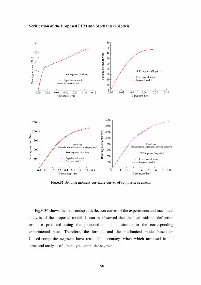
Verification of the Proposed FEM and Mechanical Models
150
0.00 0.02 0.04 0.06 0.08 0.10 0.120
10
20
30
40
50
Bend
ing
mom
ent(k
Nm
)
Curvature(1/m)
SSPC segment (Positive)
Experimental result Proposed model
0.00 0.02 0.04 0.06 0.08 0.100
20
40
60
80
100
120
140
160
180
SSPC segment (Negative)
Experimental result Proposed modelBe
ndin
g m
omen
t(kN
m)
Curvature(1/m)
0.0 0.1 0.2 0.3 0.4 0.5 0.6 0.7 0.80
500
1000
1500
2000
2500
Fourth step (No axial load and ultimate carrying capacty )
DRC segment (Positive)
Experimental result Proposed modelBe
ndin
g m
omen
t(kN
m)
Curvature(1/m) 0.0 0.1 0.2 0.3 0.4 0.5 0.6 0.7 0.80
400
800
1200
1600
2000
2400
2800
3200
Bend
ing
mom
ent(k
Nm
)
Curvature(1/m)
Fourth step (No axial load and ultimate carrying capacty )
DRC segment (Negative)
Experimental result Proposed model
Fig.6.35 Bending moment-curvature curves of composite segments
Fig.6.36 shows the load-midspan deflection curves of the experiments and mechnical
analysis of the proposed model. It can be observed that the load-midspan deflection
response predicted using the proposed model is similar to the corresponding
experimental plots. Therefore, the formula and the mechanical model based on
Closed-composite segment have reasonable accuracy, when which are used in the
structural analysis of others type composite segment.
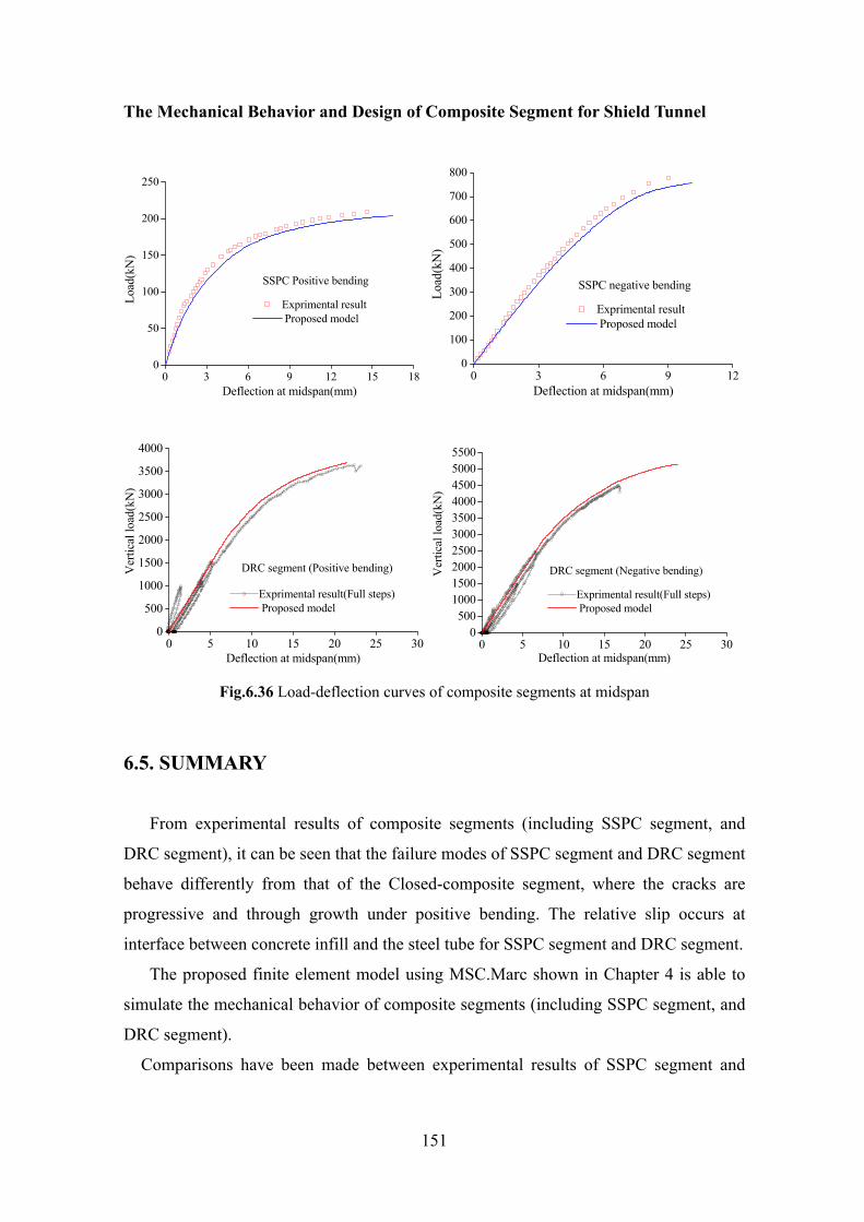
The Mechanical Behavior and Design of Composite Segment for Shield Tunnel
151
0 3 6 9 12 15 180
50
100
150
200
250
SSPC Positive bending
Load
(kN
)
Deflection at midspan(mm)
Exprimental result Proposed model
0 3 6 9 12
0
100
200
300
400
500
600
700
800
Exprimental result Proposed model
SSPC negative bending
Load
(kN
)
Deflection at midspan(mm)
0 5 10 15 20 25 300
500
1000
1500
2000
2500
3000
3500
4000
DRC segment (Positive bending)Ver
tical
load
(kN
)
Deflection at midspan(mm)
Exprimental result(Full steps) Proposed model
0 5 10 15 20 25 30
0500
1000150020002500300035004000450050005500
DRC segment (Negative bending)
Exprimental result(Full steps) Proposed model
Ver
tical
load
(kN
)
Deflection at midspan(mm) Fig.6.36 Load-deflection curves of composite segments at midspan
6.5. SUMMARY
From experimental results of composite segments (including SSPC segment, and
DRC segment), it can be seen that the failure modes of SSPC segment and DRC segment
behave differently from that of the Closed-composite segment, where the cracks are
progressive and through growth under positive bending. The relative slip occurs at
interface between concrete infill and the steel tube for SSPC segment and DRC segment.
The proposed finite element model using MSC.Marc shown in Chapter 4 is able to
simulate the mechanical behavior of composite segments (including SSPC segment, and
DRC segment).
Comparisons have been made between experimental results of SSPC segment and
Verification of the Proposed FEM and Mechanical Models
152
DRC segment and the mechanical predictions of behavior using the proposed method.
Good agreement has been found and this indicates that the method is suitable for general
analysis of others type composite segments.
6.6. REFERENCES
1) Japan Steel Segment Association (JSSA), 1995. The report of development of Steel
Segment with Pre-filled Concrete(SSPC) . (In Japanese)
2) Masami, Shirato, et al.2003. Development of new composite segment and application
to the tunneling project. Journal of JSCE, No.728, 157-174.(In Japanese)

The Mechanical Behavior and Design of Composite Segment for Shield Tunnel
153
Chapter 7. Design of Composite Segment
7.1 INTRODUCTION
Following the planning works for the tunnel, the lining of a shield tunnel (hereinafter
called as segment rings) is designed according to the following sequence, as a rule [1]:
1) Adherence to specification, and code or standard.
The tunnel to be constructed should be designed according to the appropriate
specification standard, and code or standards, which are determined by the persons in
charge of the project or decided by discussion between these persons and the designers.
2) Decision on inner dimension of tunnel.
The inner diameter of the tunnel to be designed should be decided in consideration of
the space that is demanded by the functions of the tunnel. This space is determined by:
a) The construction gauge and car gauge, in the case of railway tunnels;
b) The traffic volume and number of lanes, in the case of road tunnels;
c) The discharge, in the case of water tunnels and sewer tunnels;
d) The kind of facilities and their dimensions, in the case of common ducts.
3) Determination of load condition.
The loads acting on the lining include earth pressure and water pressure, dead load,
reaction, surcharge and thrust force of shield jacks, etc. The designer should select the
cases critical to the design lining.
4) Determination of lining conditions.
The designer should decide on the lining conditions, such as dimension of the lining
(thickness), strength of material, arrangement of reinforcement, etc.
5) Computation of member forces. The designer should compute member forces such as
bending moment, axial force, and shear force of the lining, by using appropriate models
and design methods.
6) Safety check.
The designer should check the safety of the lining against the computed member
forces.
7) Review.
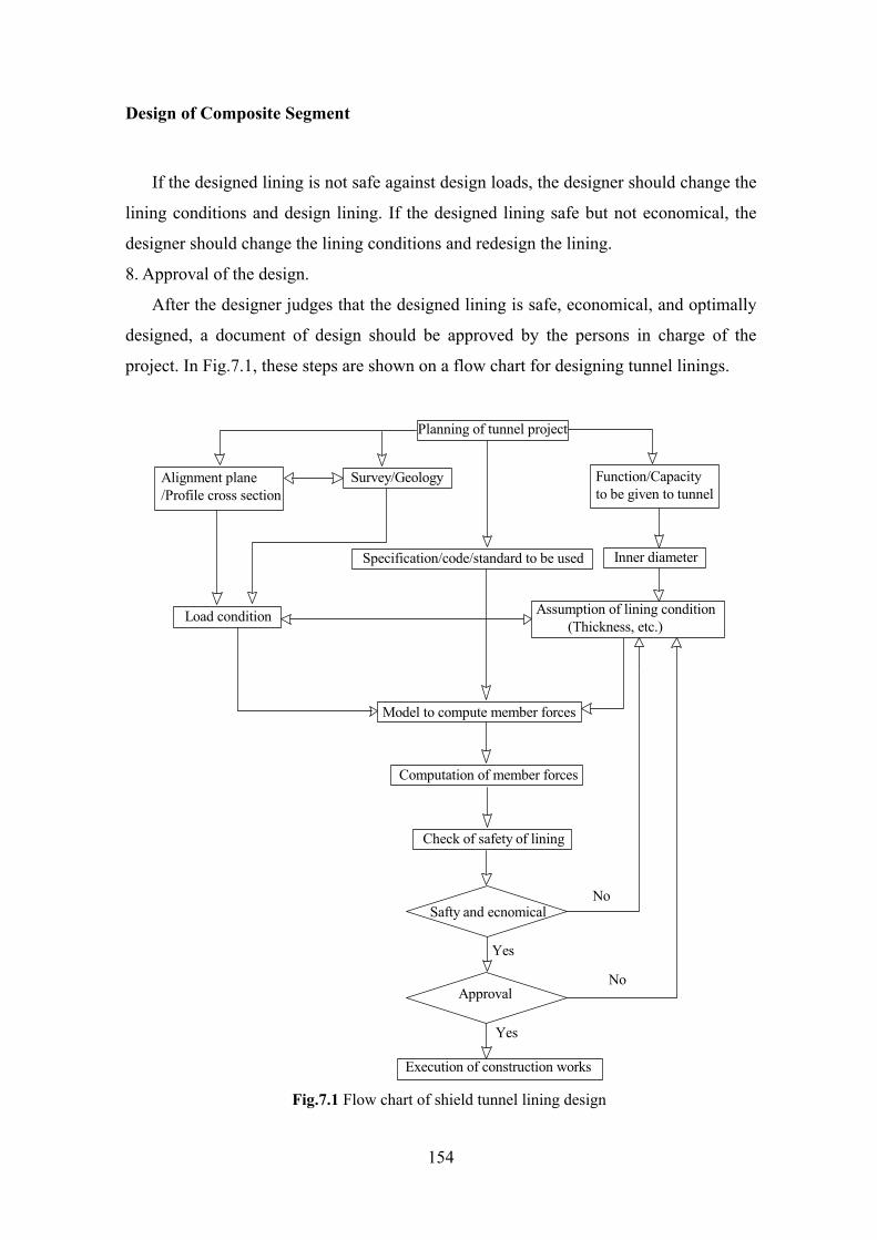
Design of Composite Segment
154
If the designed lining is not safe against design loads, the designer should change the
lining conditions and design lining. If the designed lining safe but not economical, the
designer should change the lining conditions and redesign the lining.
8. Approval of the design.
After the designer judges that the designed lining is safe, economical, and optimally
designed, a document of design should be approved by the persons in charge of the
project. In Fig.7.1, these steps are shown on a flow chart for designing tunnel linings.
No
No
Yes
Yes
Execution of construction works
Approval
Safty and ecnomical
Check of safety of lining
Computation of member forces
Model to compute member forces
Assumption of lining condition (Thickness, etc.)
Load condition
Inner diameterSpecification/code/standard to be used
Function/Capacityto be given to tunnel
Alignment plane/Profile cross section
Survey/Geology
Planning of tunnel project
Fig.7.1 Flow chart of shield tunnel lining design
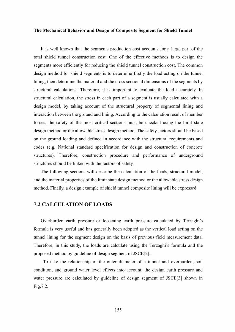
The Mechanical Behavior and Design of Composite Segment for Shield Tunnel
155
It is well known that the segments production cost accounts for a large part of the
total shield tunnel construction cost. One of the effective methods is to design the
segments more efficiently for reducing the shield tunnel construction cost. The common
design method for shield segments is to determine firstly the load acting on the tunnel
lining, then determine the material and the cross sectional dimensions of the segments by
structural calculations. Therefore, it is important to evaluate the load accurately. In
structural calculation, the stress in each part of a segment is usually calculated with a
design model, by taking account of the structural property of segmental lining and
interaction between the ground and lining. According to the calculation result of member
forces, the safety of the most critical sections must be checked using the limit state
design method or the allowable stress design method. The safety factors should be based
on the ground loading and defined in accordance with the structural requirements and
codes (e.g. National standard specification for design and construction of concrete
structures). Therefore, construction procedure and performance of underground
structures should be linked with the factors of safety.
The following sections will describe the calculation of the loads, structural model,
and the material properties of the limit state design method or the allowable stress design
method. Finally, a design example of shield tunnel composite lining will be expressed.
7.2 CALCULATION OF LOADS
Overburden earth pressure or loosening earth pressure calculated by Terzaghi’s
formula is very useful and has generally been adopted as the vertical load acting on the
tunnel lining for the segment design on the basis of previous field measurement data.
Therefore, in this study, the loads are calculate using the Terzaghi’s formula and the
proposed method by guideline of design segment of JSCE[2].
To take the relationship of the outer diameter of a tunnel and overburden, soil
condition, and ground water level effects into account, the design earth pressure and
water pressure are calculated by guideline of design segment of JSCE[3] shown in
Fig.7.2.
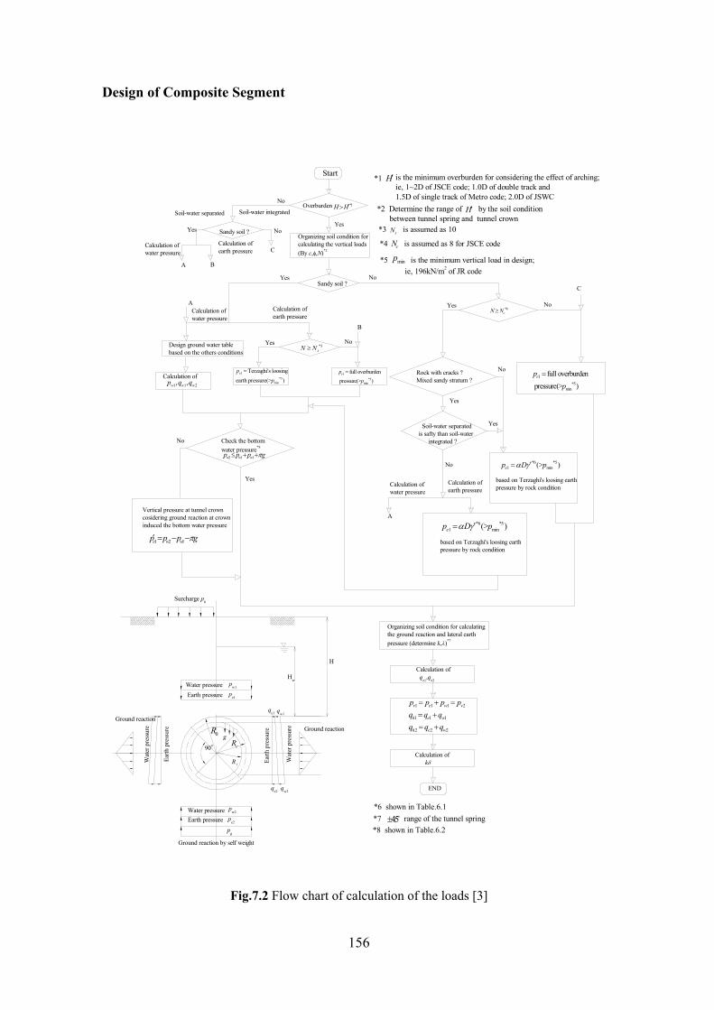
Design of Composite Segment
156
*8 shown in Table.6.245±*7 range of the tunnel spring
*6 shown in Table.6.1
minp*5 is the minimum vertical load in design; ie, 196kN/m2 of JR code
cN*4 is assumed as 8 for JSCE codesN*3 is assumed as 10
H′*2 Determine the range of by the soil condition between tunnel spring and tunnel crown
is the minimum overburden for considering the effect of arching;ie, 1~2D of JSCE code; 1.0D of double track and1.5D of single track of Metro code; 2.0D of JSWC
H′*1
Calculation of water pressure
Calculation of earth pressure
based on Terzaghi's loosing earthpressure by rock condition
based on Terzaghi's loosing earthpressure by rock condition
*6 *51 min(> )ep D pα γ′=
*6 *51 min(> )ep D pα γ ′=No
Soil-water separated is safty than soil-water integrated ?
Rock with cracks ?Mixed sandy stratum ?
1
*5min
full overburden pressure(> )
epp
=
No
No
Yes
Yes
Yes
A
Organizing soil condition for calculating the ground reaction and lateral earth pressure (determine k,λ)*7
Calculation of q
e1,q
e2
1 1 1 2
1 1 1
2 2 2
v e w v
h e w
h e w
p p p pq q qq q q
= + == += +
Calculation of kδ
ENDqw2
qe2
qe1 q
w1
0RcR
iR
H
Hw
Ground reaction
Wat
er p
ress
ure
Earth
pre
ssur
e
Earth
pre
ssur
e
Wat
er p
ress
ure
90o
g
pg
Ground reaction by self weight
pe2Earth pressure
pw2Water pressure
Ground reaction
pe1Earth pressure
pw1Water pressure
Surcharge p0
1 2 1e w wp p p gπ′ = − −
Vertical pressure at tunnel crowncosidering ground reaction at crowninduced the bottom water pressure
2 1 1w w wp p p gπ≤ + +
Check the bottom water pressure*8
1*5
min
full overburdenpressure(> )
epp
=1*5
min
Terzaghi's loosing
earth pressure(> )ep
p
=
A
1 1 2, ,w w wp q qCalculation of
Design ground water tablebased on the others conditions
NoYes*4
cN N≥
*3sN N≥
NoYes
C
B
Calculation of earth pressure
Calculation of water pressure
NoYesSandy soil ?
Calculation of earth pressure
Calculation of water pressure C
BA
NoYesOrganizing soil condition forcalculating the vertical loads(By c,φ,N)*2
Yes
No
Sandy soil ?
Soil-water separated Soil-water integrated*1H H′>Overburden
Start
Fig.7.2 Flow chart of calculation of the loads [3]
The Mechanical Behavior and Design of Composite Segment for Shield Tunnel
157
Table 7.1. Earth pressure acting on the lining by Terzaghi[4]
Rock condition Rock load factor H(m) Remarks
(1) Hard and intact 0 Simple support may be required
(2) Hard, stratified or schistose
0~0.25B
(3) Massive, moderately jointed
0~0.5B
Simple support may be required; nonuniformly varying load
(4) Moderately blocky, seamy and jointed
0~0.25B;0.35(B+Ht) lateral earth pressure is equal to zero
(5) Very blocky and seamy, shattered
(0.35~1.10)(B+Ht) lateral earth pressure is very little or equal to zero;
(6) Completely crushed but chemically intact
1.10(B+Ht) Inverts essential, arched roof essential
(7) Squeezing rock at moderate depth
(1.10~1.0)(B+Ht)
(8) Squeezing rock at great depth
(2.10~4.5)(B+Ht)
Inverts essential in excavation, arched roof essential
(9) Swelling rock Up to 80m irrespective of (B+Ht)Inverts essential in excavation, arched roof essential
Note: 1) The table shows the rock load factor for overburden up to 1.5(B+Ht) B is width or span of opening; Ht is height of opening
2) The table shows tunnel is located below groundwater table. If tunnel is located above groundwater table, the value of (6) reduces 50%.
Table 7.2. Coefficient (λ ) of lateral earth pressure and coefficient ( k ) of ground reaction [5]
k (MN/m3) Type of soil λ
During grouted After grouted
N value
guideline
Very dense sandy soil 0.35-0.45 35.0-47.0 55.0-90.0 30N ≤
Dense sandy soil 0.45-0.50 21.5-35.0 28.0-55.0 15 30N≤ <
Medium, loose sandy soil 0.50-0.60 21.5 28.0 15N <
Hard clayey soil 0.40-0.50 31.5 41.0 8 25N≤ ≤
Medium and stiff clayey soil 0.50-0.60 13.0-31.5 15.0-46.0 4 8N≤ <
Soft clayey soil 0.60-0.70 3.5-7.0 3.8-7.5 2 4N≤ <
Very soft clayey soil 0.70-0.80 3.5 3.8 2N <

Design of Composite Segment
158
0p
γ′
cφ
cφ
γ
vσ
1vσ
wH
H WL
12B
45 /2φ°+
2φ
1φ1c
2c
1γ
245 /2φ°+
2γ
H2
0p
vσ
1vσH1
12B
(a) Single soil strata with ground water (b) Alternation of strata
Fig.7.3 Calculation model of loosing earth pressure
7.2.1 Earth Pressure and Water Pressure Earth pressure and water pressure are calculate by flow chart of calculation of the
loads (Fig.7.2) shown in Table 7.3 and Table 7.4.
(1) Loosing earth pressure by Terzaghi’s formula
Loosing earth pressure for Single soil strata with ground water shown in Fig.7.3(a) is
calculated as
( ) ( )0 1 0 1/ tan / tan1 10
0
/1
tanK H B K H B
v
B c Be p e
Kφ φγ
σφ
− −−= − + (7.1)
1 0/ 4 / 2cot
2B R π φ+⎛ ⎞= ⎜ ⎟
⎝ ⎠ (7.2)
where, vσ is loosing earth pressure; 0K is Ratio between lateral earth pressure and
vertical earth pressure(equal to 1);φ is angle of internal friction of soil; 0p is surcharge;
c is cohesion of soil; γ is unit weight of soil; and 0R is outer radius of the lining.

The Mechanical Behavior and Design of Composite Segment for Shield Tunnel
159
(2) Loosing earth pressure of below ground water table (a) wH H<
( ) ( )0 1 0 1( ) / tan ( ) / tan1 11 0
0
/1
tanw wK H H B K H H B
v
B c Be p e
Kφ φγ
σφ
− − − −−= − + (7.3)
( ) ( )
( ) ( )
( ) ( )
( ) ( )
0 1 0 1
0 1 0 1 0 1
0 1
0 1 0 1
/ tan / tan1 11
0
( ) / tan ( ) / tan / tan1 10
0
/ tan1 1
0
/ tan / tan1 10
0
/1
tan
/1
tan
/1
tan/
1tan
w w
w w w
w
w
K H B K H Bv v
K H H B K H H B K H B
K H B
K H B K H B
B c Be e
K
B c Be p e e
K
B c Be
KB c B
e p eK
φ φ
φ φ φ
φ
φ φ
γσ σ
φ
γφ
γφ
γφ
− −
− − − − −
−
− −
′ −= − +
⎧ ⎫−= − +⎨ ⎬⎩ ⎭
′ −+ −
′ −= − +
( ) ( )0 1 0 1( ) / tan / tan1 1
0
/1
tanw wK H H B K H BB c B
e eK
φ φγφ
− − −−+ −
(7.4)
(b) wH H≥
( ) ( )0 1 0 1/ tan / tan1 10
0
/1
tanK H B K H B
v
B c Be p e
Kφ φγ
σφ
− −′ −= − + (7.5)
where, 1 0/ 4 / 2cot
2B R π φ+⎛ ⎞= ⎜ ⎟
⎝ ⎠.
(3) Loosing earth pressure for alternation of strata
Loosing earth pressure of alternation of strata shown in Fig.7.3(b) is calculated as
( ) ( )0 1 1 1 0 1 1 1/ tan / tan1 1 1 11 0
0 1
/1
tanK H B K H B
v
B c Be p e
Kφ φγ
σφ
− −−= − + (7.6)
( ) ( )
( ) ( )
( ) ( ) ( )
0 2 1 2 0 2 1 2
0 2 1 2
0 1 1 1 0 2 1 2
0 1 1 2 2 1
/ tan / tan1 2 2 11 1
0 2
/ tan1 2 2 1
0 2
/ tan / tan1 1 1 1
0 1( tan tan ) /
0
/1
tan/
1tan
/1 1
tan
K H B K H Bv v
K H B
K H B K H B
K H H B
B c Be e
KB c B
eK
B c Be e
K
p e
φ φ
φ
φ φ
φ φ
γσ σ
φγ
φγ
φ
− −
−
− −
− +
−= − +
−= −
−+ − −
+
(7.7)
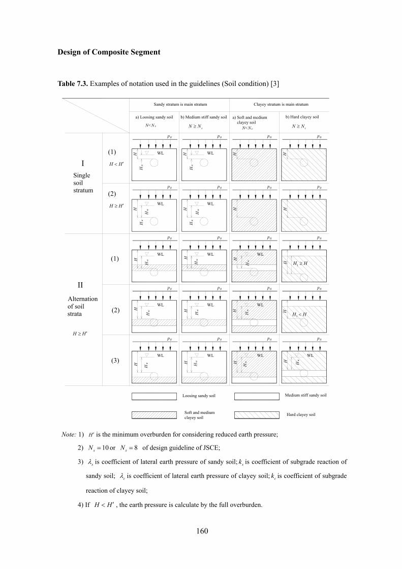
Design of Composite Segment
160
Table 7.3. Examples of notation used in the guidelines (Soil condition) [3]
1H H≥
1H H<
Sandy stratum is main stratum Clayey stratum is main stratum
a) Loosing sandy soil
N<N s
b) Medium stiff sandy soil
HH
w
H H H
H H H H
Hw
Hw
Hw
a) Soft and medium clayey soil
N<N c
b) Hard clayey soil
p0 p0 p0 p0
p0 p0 p0 p0
p0 p0 p0 p0
p0 p0 p0 p0
p0 p0 p0 p0
WLWL
WL WL
WL WLWL
WLWLWL
WL WL WL WL
Loosing sandy soil Medium stiff sandy soil
Soft and medium clayey soil
Hard clayey soil
Single soilstratum
Alternation of soilstrata
H H
H
HH H
HHHHH H
Hw
Hw
HwHw
Hw
Hw
Hw
Hw
Hw
Hw
Hw H
w
І
II
(1)
H H ′<
(1)
(2)
(3)
(2)
H H ′≥
sN N≥ cN N≥
H H ′≥
Note: 1) H ′ is the minimum overburden for considering reduced earth pressure;
2) 10sN = or 8sN = of design guideline of JSCE;
3) sλ is coefficient of lateral earth pressure of sandy soil; sk is coefficient of subgrade reaction of
sandy soil; cλ is coefficient of lateral earth pressure of clayey soil; ck is coefficient of subgrade
reaction of clayey soil;
4) If H H ′< , the earth pressure is calculate by the full overburden.
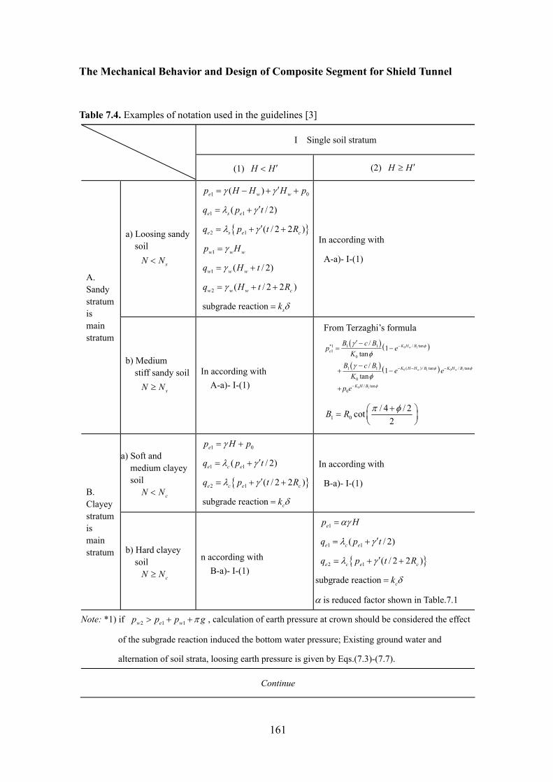
The Mechanical Behavior and Design of Composite Segment for Shield Tunnel
161
Table 7.4. Examples of notation used in the guidelines [3]
I Single soil stratum
(1) H H ′< (2) H H ′≥
a) Loosing sandy soil
sN N<
1 0( )e w wp H H H pγ γ ′= − + +
1 1( / 2)e s eq p tλ γ ′= +
{ }2 1 ( / 2 2 )e s e cq p t Rλ γ ′= + +
1w w wp Hγ=
1 ( / 2)w w wq H tγ= +
2 ( / 2 2 )w w w cq H t Rγ= + +
subgrade reaction sk δ=
In according with
A-a)- I-(1)
A. Sandy stratum is main stratum
b) Medium stiff sandy soil
sN N≥
In according with A-a)- I-(1)
From Terzaghi’s formula ( ) ( )
( ) ( )
0 1
0 1 0 1
0 1
/ tan*1 1 11
0
( ) / tan / tan1 1
0/ tan
0
/1
tan/
1tan
w
w w
K H Be
K H H B K H B
K H B
B c Bp e
KB c B
e eK
p e
φ
φ φ
φ
γφ
γφ
−
− − −
−
′ −= −
−+ −
+
1 0/ 4 / 2cot
2B R π φ+⎛ ⎞= ⎜ ⎟
⎝ ⎠
a) Soft and medium clayey soil
cN N<
1 0ep H pγ= +
1 1( / 2)e c eq p tλ γ ′= +
{ }2 1 ( / 2 2 )e c e cq p t Rλ γ ′= + +
subgrade reaction ck δ=
In according with
B-a)- I-(1) B. Clayey stratum is main stratum b) Hard clayey
soil cN N≥
n according with B-a)- I-(1)
1ep Hαγ=
1 1( / 2)e c eq p tλ γ ′= +
{ }2 1 ( / 2 2 )e c e cq p t Rλ γ ′= + +
subgrade reaction ck δ=
α is reduced factor shown in Table.7.1
Note: *1) if 2 1 1w e wp p p gπ> + + , calculation of earth pressure at crown should be considered the effect
of the subgrade reaction induced the bottom water pressure; Existing ground water and
alternation of soil strata, loosing earth pressure is given by Eqs.(7.3)-(7.7).
Continue
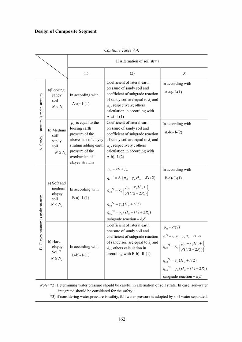
Design of Composite Segment
162
Continue Table 7.4.
II Alternation of soil strata
(1) (2) (3)
a)Loosing sandy
soil
sN N<
In according with
A-a)- I-(1)
Coefficient of lateral earth pressure of sandy soil and coefficient of subgrade reaction of sandy soil are equal to cλ and
ck , respectively; others calculation in according with A-a)- I-(1)
In according with
A-a)- I-(1)
A. S
andy
st
ratu
m is
mai
n st
ratu
m
b) Medium stiff
sandy soil
sN N≥
1ep is equal to the loosing earth pressure of the above side of clayey stratum adding earth pressure of the overburden of clayey stratum
Coefficient of lateral earth pressure of sandy soil and coefficient of subgrade reaction of sandy soil are equal to cλ and
ck , respectively ; others calculation in according with A-b)- I-(2)
In according with
A-b)- I-(2)
a) Soft and medium clayey soil
cN N<
In according with
B-a)- I-(1)
1 0ep H pγ= +
*21 1( / 2)e s e w wq p H tλ γ λ′= − +
1*22 ( / 2 2 )
e w we s
c
p Hq
t Rγ
λγ
− +⎧ ⎫= ⎨ ⎬′ +⎩ ⎭
*21 ( / 2)w w wq H tγ= +
*22 ( / 2 2 )w w w cq H t Rγ= + +
subgrade reaction sk δ=
In according with
B-a)- I-(1)
B. C
laye
y st
ratu
m is
mai
n st
ratu
m
b) Hard clayey Soil*3
cN N≥
In according with
B-b)- I-(1)
Coefficient of lateral earth pressure of sandy soil and coefficient of subgrade reaction of sandy soil are equal to cλ and
ck , others calculation in according with B-b)- II-(1)
1ep Hαγ=
*21 1( / 2)e s e w wq p H tλ γ λ′= − +
1*22 ( / 2 2 )
e w we s
c
p Hq
t Rγ
λγ
− +⎧ ⎫= ⎨ ⎬′ +⎩ ⎭
*21 ( / 2)w w wq H tγ= +
*22 ( / 2 2 )w w w cq H t Rγ= + +
subgrade reaction sk δ=
Note: *2) Determining water pressure should be careful in alternation of soil strata. In case, soil-water integrated should be considered for the safety;
*3) if considering water pressure is safety, full water pressure is adopted by soil-water separated.
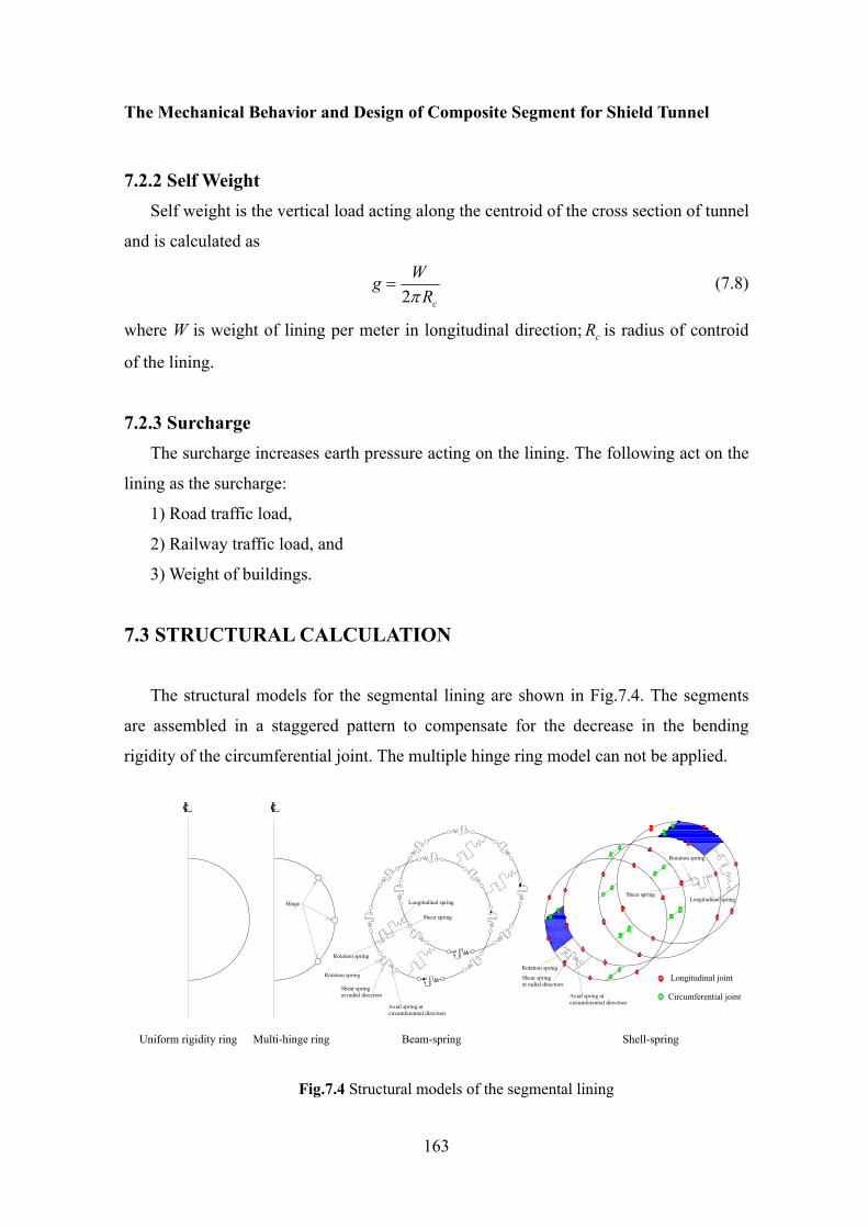
The Mechanical Behavior and Design of Composite Segment for Shield Tunnel
163
7.2.2 Self Weight Self weight is the vertical load acting along the centroid of the cross section of tunnel
and is calculated as
2 c
WgRπ
= (7.8)
where W is weight of lining per meter in longitudinal direction; cR is radius of controid
of the lining.
7.2.3 Surcharge The surcharge increases earth pressure acting on the lining. The following act on the
lining as the surcharge:
1) Road traffic load,
2) Railway traffic load, and
3) Weight of buildings.
7.3 STRUCTURAL CALCULATION
The structural models for the segmental lining are shown in Fig.7.4. The segments
are assembled in a staggered pattern to compensate for the decrease in the bending
rigidity of the circumferential joint. The multiple hinge ring model can not be applied.
Uniform rigidity ring Multi-hinge ring Beam-spring Shell-spring
Hinge
cL cL
Rotation spring
Shear spring at radial direction
Axial spring at circumferential direction
Longitudinal spring
Shear spring at radial direction
Axial spring at circumferential direction
Rotation spring
Shear spring
Rotation spring
Rotation spring
Longitudinal spring Shear spring
Circumferential joint
Longitudinal joint
Fig.7.4 Structural models of the segmental lining
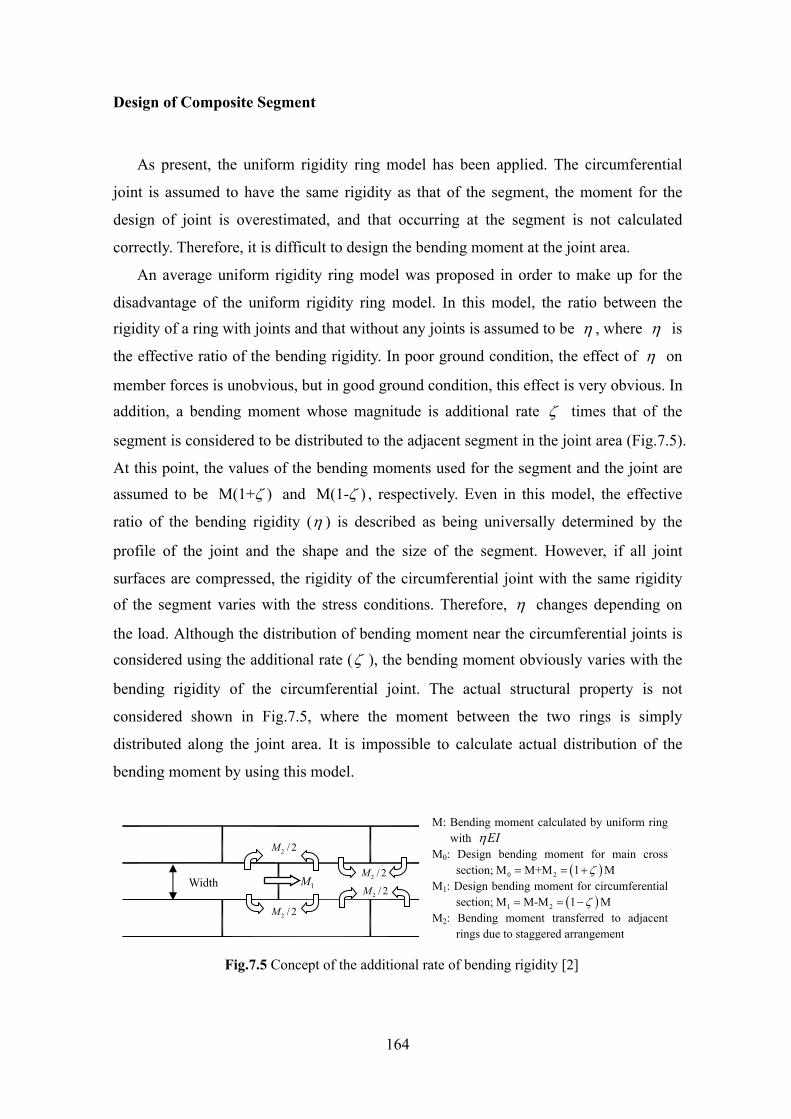
Design of Composite Segment
164
As present, the uniform rigidity ring model has been applied. The circumferential
joint is assumed to have the same rigidity as that of the segment, the moment for the
design of joint is overestimated, and that occurring at the segment is not calculated
correctly. Therefore, it is difficult to design the bending moment at the joint area.
An average uniform rigidity ring model was proposed in order to make up for the
disadvantage of the uniform rigidity ring model. In this model, the ratio between the rigidity of a ring with joints and that without any joints is assumed to be η , where η is
the effective ratio of the bending rigidity. In poor ground condition, the effect of η on
member forces is unobvious, but in good ground condition, this effect is very obvious. In addition, a bending moment whose magnitude is additional rate ζ times that of the
segment is considered to be distributed to the adjacent segment in the joint area (Fig.7.5).
At this point, the values of the bending moments used for the segment and the joint are assumed to be M(1+ )ζ and M(1- )ζ , respectively. Even in this model, the effective
ratio of the bending rigidity (η ) is described as being universally determined by the
profile of the joint and the shape and the size of the segment. However, if all joint
surfaces are compressed, the rigidity of the circumferential joint with the same rigidity of the segment varies with the stress conditions. Therefore, η changes depending on
the load. Although the distribution of bending moment near the circumferential joints is considered using the additional rate (ζ ), the bending moment obviously varies with the
bending rigidity of the circumferential joint. The actual structural property is not
considered shown in Fig.7.5, where the moment between the two rings is simply
distributed along the joint area. It is impossible to calculate actual distribution of the
bending moment by using this model.
Fig.7.5 Concept of the additional rate of bending rigidity [2]
M: Bending moment calculated by uniform ring with EIη
M0: Design bending moment for main cross section; ( )0 2M M+M 1 Mζ= = +
M1: Design bending moment for circumferential section; ( )1 2M M-M 1 Mζ= = −
M2: Bending moment transferred to adjacent rings due to staggered arrangement
Width
2 / 2M
2 / 2M
1M2 / 2M
2 / 2M

The Mechanical Behavior and Design of Composite Segment for Shield Tunnel
165
For the above reason, the beam-spring model and the shell-spring were proposed
and applied in design of segmental lining nowadays. In the beam spring model,
segments are modeled using beams. The circumferential joints are modeled using the
rotation of springs and their rigidities are expressed by the constants of the springs
concerning the bending moments. The longitudinal joints are modeled using shear
springs to simulate the relative displacement occurring between the two adjacent rings in
the longitudinal direction. However, the bending moment distribution along the width of
a ring is non-uniform due to the split effect of the longitudinal joints. Therefore, the
shell-spring model is applied, in which tunnel lining is modeled using shell, and the
joints are modeled using springs.
7.3.1 Elastic Equation Method The tunnel is assumed to be made of a rigid material and the soil reaction is
determined to be independent of the tunnel deformation caused by active loads. This
model is called the ‘conventional model’/ the ‘modified conventional model’ shown in
Fig.7.2, and the calculations of member force based on elastic equation method is given
by Table 7.5
Table 7.5. Equations of member forces for conventional model/ modified conventional model[3]
Load Bending moment Axial force Shear force
Uniform load in vertical direction
1 1( )e wp p+
21 1
1 (1 2S)( )4 e w cM p p R= − +
1 1( ) S2e w cN p p R= + 1 1( ) SCe w cQ p p R= − +
Uniform load in lateral direction
1 1( )e wq q+ 2
1 11 (1 2C2)( )4 e w cM q q R= − +
1 1( ) C2e w cN q q R= + 1 1( ) SCe w cQ q q R= +
Triangularly varying load in lateral direction
2 2 1 1( )e w e wq q q q+ − − 22 2 1 1
1 (6 3C 12C2 4C3)48
( )e w e w c
M
q q q q R
= − − +
+ − −
2 2 1 1
1 (C 8C2 4C3)16
( )e w e w c
N
q q q q R
= + −
+ − − 2 2 1 1
1 (S 8SC 4SC2)16
( )e w e w c
Q
q q q q R
= + −
+ − −
Subgrade reaction in lateral direction
( )kδ 0
4πθ≤ <
2(0.2346 0.3536C) cM k Rδ= −
04πθ≤ <
0.3536C cN k Rδ=
04πθ≤ <
0.3536S cQ k Rδ=
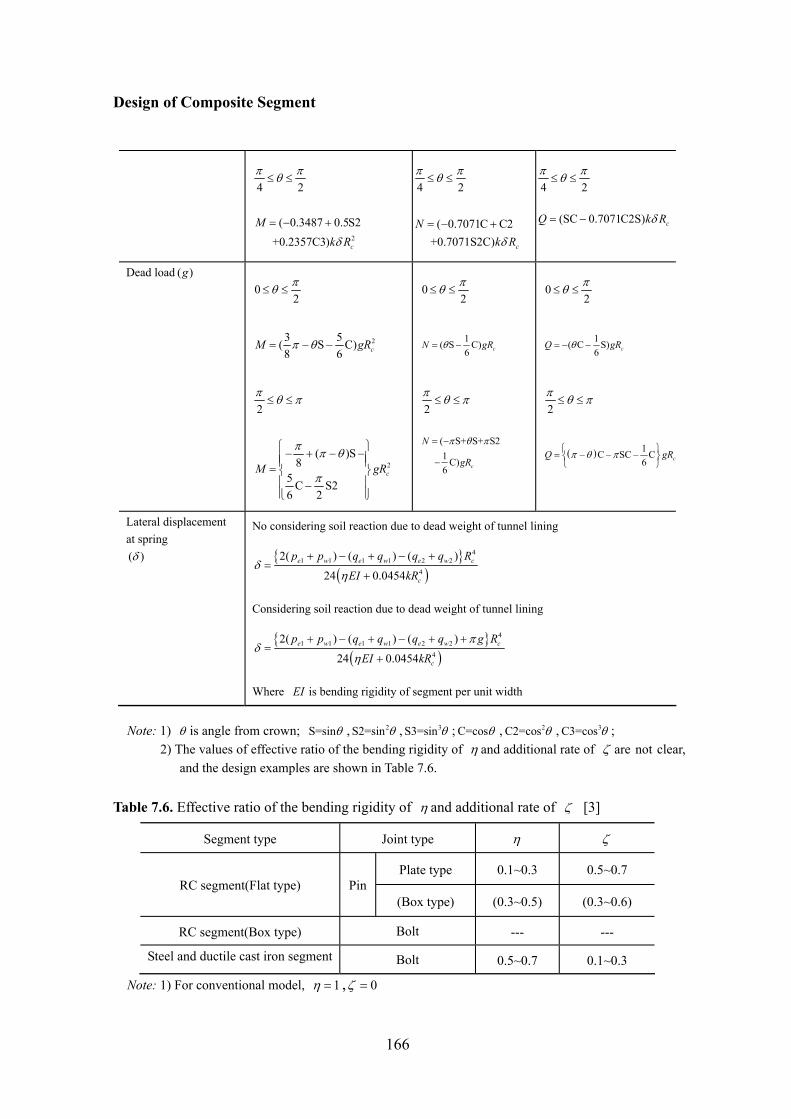
Design of Composite Segment
166
4 2π πθ≤ ≤
2
( 0.3487 0.5S2+0.2357C3) c
Mk Rδ
= − +
4 2π πθ≤ ≤
( 0.7071C C2+0.7071S2C) c
Nk Rδ
= − +
4 2π πθ≤ ≤
(SC 0.7071C2S) cQ k Rδ= −
Dead load ( )g 0
2πθ≤ ≤
23 5( S C)8 6 cM gRπ θ= − −
2π θ π≤ ≤
2( )S
85 C S26 2
cM gR
π π θ
π
⎧ ⎫− + − −⎪ ⎪⎪ ⎪= ⎨ ⎬⎪ ⎪−⎪ ⎪⎩ ⎭
02πθ≤ ≤
1( S C)6 cN gRθ= −
2π θ π≤ ≤
( S+ S+ S21 C)6 c
N
gR
π θ π= −
−
02πθ≤ ≤
1( C S)6 cQ gRθ= − −
2π θ π≤ ≤
( ) 1C SC C6 cQ gRπ θ π⎧ ⎫= − − −⎨ ⎬
⎩ ⎭
Lateral displacement at spring ( )δ
No considering soil reaction due to dead weight of tunnel lining
{ }( )
41 1 1 1 2 2
4
2( ) ( ) ( )
24 0.0454e w e w e w c
c
p p q q q q R
EI kRδ
η
+ − + − +=
+
Considering soil reaction due to dead weight of tunnel lining
{ }( )
41 1 1 1 2 2
4
2( ) ( ) ( )
24 0.0454e w e w e w c
c
p p q q q q g R
EI kR
πδ
η
+ − + − + +=
+
Where EI is bending rigidity of segment per unit width
Note: 1) θ is angle from crown; S=sinθ , 2S2=sin θ , 3S3=sin θ ; C=cosθ , 2C2=cos θ , 3C3=cos θ ; 2) The values of effective ratio of the bending rigidity of η and additional rate of ζ are not clear,
and the design examples are shown in Table 7.6.
Table 7.6. Effective ratio of the bending rigidity of η and additional rate of ζ [3]
Segment type Joint type η ζ
Plate type 0.1~0.3 0.5~0.7 RC segment(Flat type) Pin
(Box type) (0.3~0.5) (0.3~0.6)
RC segment(Box type) Bolt --- ---
Steel and ductile cast iron segment Bolt 0.5~0.7 0.1~0.3
Note: 1) For conventional model, 1η = , 0ζ =
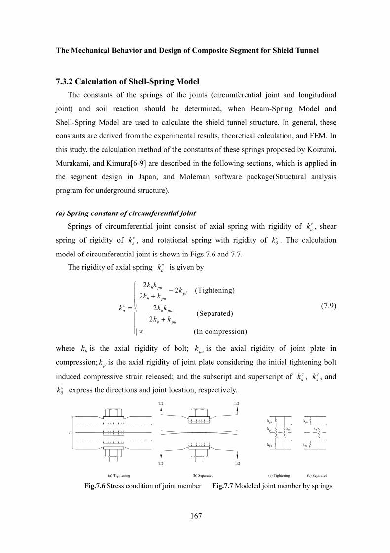
The Mechanical Behavior and Design of Composite Segment for Shield Tunnel
167
7.3.2 Calculation of Shell-Spring Model
The constants of the springs of the joints (circumferential joint and longitudinal
joint) and soil reaction should be determined, when Beam-Spring Model and
Shell-Spring Model are used to calculate the shield tunnel structure. In general, these
constants are derived from the experimental results, theoretical calculation, and FEM. In
this study, the calculation method of the constants of these springs proposed by Koizumi,
Murakami, and Kimura[6-9] are described in the following sections, which is applied in
the segment design in Japan, and Moleman software package(Structural analysis
program for underground structure).
(a) Spring constant of circumferential joint
Springs of circumferential joint consist of axial spring with rigidity of cak , shear
spring of rigidity of csk , and rotational spring with rigidity of ckθ . The calculation
model of circumferential joint is shown in Figs.7.6 and 7.7.
The rigidity of axial spring cak is given by
22 (Tightening)
2 2
(Separated)2
(In compression)
b pupl
b puca b pu
b pu
k kk
k kk k k
k k
⎧+⎪ +⎪⎪= ⎨
⎪ +⎪⎪∞⎩
(7.9)
where bk is the axial rigidity of bolt; puk is the axial rigidity of joint plate in
compression; plk is the axial rigidity of joint plate considering the initial tightening bolt
induced compressive strain released; and the subscript and superscript of cak , c
sk , and ckθ express the directions and joint location, respectively.
2t
T/2 T/2
T/2 T/2
kpu
kpu
kpL kb
kpu
kb
kpu
(a) Tightening (b) Separated (a) Tightening (b) Separated Fig.7.6 Stress condition of joint member Fig.7.7 Modeled joint member by springs
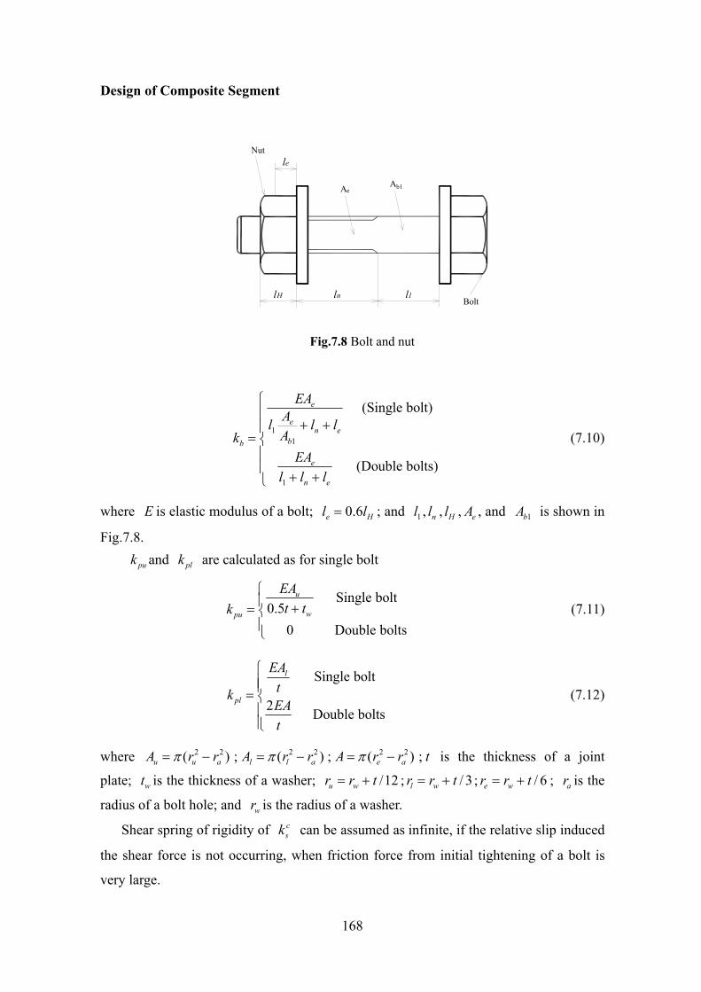
Design of Composite Segment
168
lH
le
ln l1
AeAb1
Nut
Bolt
Fig.7.8 Bolt and nut
11
1
(Single bolt)
(Double bolts)
e
en e
bb
e
n e
EAAl l lAk
EAl l l
⎧⎪
+ +⎪= ⎨⎪⎪
+ +⎩
(7.10)
where E is elastic modulus of a bolt; 0.6e Hl l= ; and 1l , nl , Hl , eA , and 1bA is shown in
Fig.7.8.
puk and plk are calculated as for single bolt
Single bolt0.5
0 Double bolts
u
wpu
EAt tk
⎧⎪ += ⎨⎪⎩
(7.11)
Single bolt
2 Double bolts
l
pl
EAtkEAt
⎧⎪⎪= ⎨⎪⎪⎩
(7.12)
where 2 2( )u u aA r rπ= − ; 2 2( )l l aA r rπ= − ; 2 2( )e aA r rπ= − ; t is the thickness of a joint
plate; wt is the thickness of a washer; /12u wr r t= + ; / 3l wr r t= + ; / 6e wr r t= + ; ar is the
radius of a bolt hole; and wr is the radius of a washer.
Shear spring of rigidity of csk can be assumed as infinite, if the relative slip induced
the shear force is not occurring, when friction force from initial tightening of a bolt is
very large.
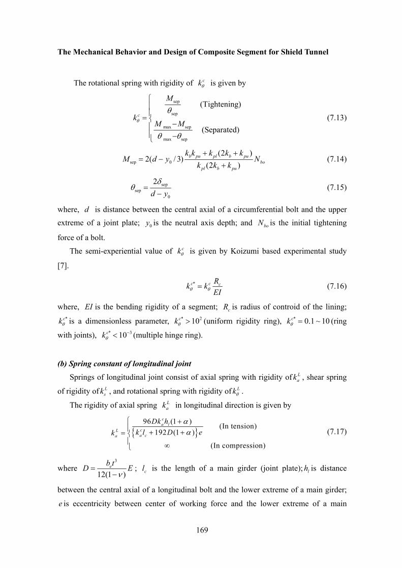
The Mechanical Behavior and Design of Composite Segment for Shield Tunnel
169
The rotational spring with rigidity of ckθ is given by
sep
sep
max sep
max sep
(Tightening)
(Separated)
c
M
kM Mθ
θ
θ θ
⎧⎪⎪= ⎨ −⎪⎪ −⎩
(7.13)
sep 0
(2 )2( / 3)
(2 )b pu pl b pu
bopl b pu
k k k k kM d y N
k k k+ +
= −+
(7.14)
sepsep
0
2d yδ
θ =−
(7.15)
where, d is distance between the central axial of a circumferential bolt and the upper extreme of a joint plate; 0y is the neutral axis depth; and boN is the initial tightening
force of a bolt.
The semi-experiential value of ckθ is given by Koizumi based experimental study
[7].
* c c cRk kEIθ θ= (7.16)
where, EI is the bending rigidity of a segment; cR is radius of controid of the lining; *ckθ is a dimensionless parameter, * 210ckθ > (uniform rigidity ring), * 0.1 ~ 10ckθ = (ring
with joints), * 310ckθ−< (multiple hinge ring).
(b) Spring constant of longitudinal joint
Springs of longitudinal joint consist of axial spring with rigidity of Lak , shear spring
of rigidity of Lsk , and rotational spring with rigidity of Lkθ .
The rigidity of axial spring Lak in longitudinal direction is given by
{ }96 (1 ) (In tension)
192 (1 )
(In compression)
ca l
cLa ca
Dk hk l D ek
αα
⎧ +⎪ + += ⎨⎪ ∞⎩
(7.17)
where 3
12(1 )eb tD Eν
=−
; cl is the length of a main girder (joint plate); lh is distance
between the central axial of a longitudinal bolt and the lower extreme of a main girder;
e is eccentricity between center of working force and the lower extreme of a main
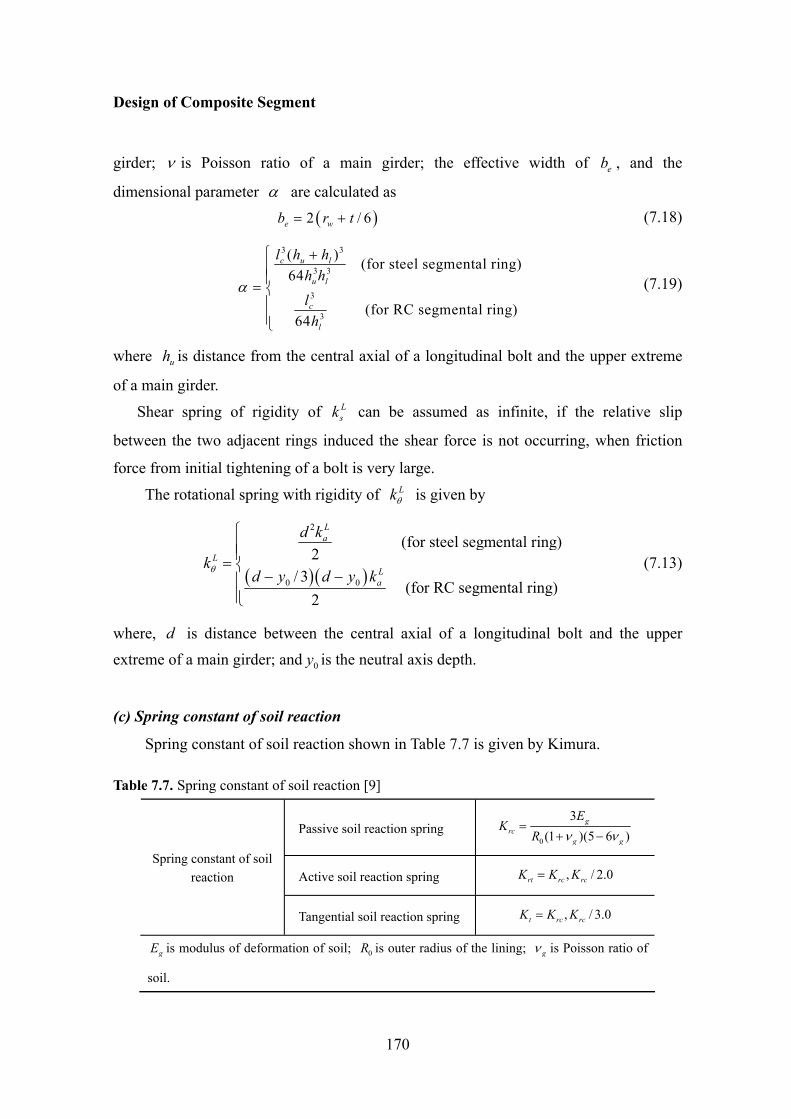
Design of Composite Segment
170
girder; ν is Poisson ratio of a main girder; the effective width of eb , and the
dimensional parameter α are calculated as
( )2 / 6e wb r t= + (7.18)
3 3
3 3
3
3
( ) (for steel segmental ring)64
(for RC segmental ring)64
c u l
u l
c
l
l h hh h
lh
α
⎧ +⎪⎪= ⎨⎪⎪⎩
(7.19)
where uh is distance from the central axial of a longitudinal bolt and the upper extreme
of a main girder.
Shear spring of rigidity of Lsk can be assumed as infinite, if the relative slip
between the two adjacent rings induced the shear force is not occurring, when friction
force from initial tightening of a bolt is very large.
The rotational spring with rigidity of Lkθ is given by
( ) ( )
2
0 0
(for steel segmental ring)2
/ 3(for RC segmental ring)
2
La
LLa
d k
kd y d y kθ
⎧⎪⎪= ⎨
− −⎪⎪⎩
(7.13)
where, d is distance between the central axial of a longitudinal bolt and the upper extreme of a main girder; and 0y is the neutral axis depth.
(c) Spring constant of soil reaction
Spring constant of soil reaction shown in Table 7.7 is given by Kimura.
Table 7.7. Spring constant of soil reaction [9]
Passive soil reaction spring 0
3(1 )(5 6 )
grc
g g
EK
R ν ν=
+ −
Active soil reaction spring , / 2.0rt rc rcK K K= Spring constant of soil
reaction
Tangential soil reaction spring , / 3.0t rc rcK K K=
gE is modulus of deformation of soil; 0R is outer radius of the lining; gν is Poisson ratio of
soil.

The Mechanical Behavior and Design of Composite Segment for Shield Tunnel
171
7.4 CHECK OF SAFETY OF SEGMENTAL LINING
According to the calculation result of member forces, the safety of the most critical
sections must be checked using the limit state design method or the allowable stress
design method. These are as follows:
1) Section with the maximum positive moment.
2) Section with the maximum negative moment.
3) Section with the maximum axial force.
The safety of the lining against the thrust force of the shield jacks should be checked.
7.4.1 Allowable Stress Design Method The allowable stresses in lining materials are described as the following sections [2].
(a) Concrete for segment
Allowable stresses of concrete for segment are shown in Table 7.8.
Table 7.8. Allowable stresses of concrete for segment (N/mm2) [2]
Characteristic compressive strength ckσ 42 45 48 51 54 57 60
Allowable compressive stress for bending moment caσ 16 17 18 19 20 21 22Allowable standard shear stress Shear stress by bending1) aτ 0.73 0.74 0.76 0.78 0.79 0.81 0.82
Allowable bond stress(deformed bar) 0τ 2.0 2.1 2.1 2.2 2.2 2.3 2.3
Overall loading baσ 15 16 17 18 18 20 21Allowable carrying stress
Local loading2) baσ 1/ 2.8ba ck aA Aσ σ≤ ⋅ and ba ckσ σ≤
Note: 1) aτ is calculated by the effective height for a segment of d=20cm and tensional reinforcement ratio=1%, therefore, aτ must be adjusted as follows:
a) Adjustment for different effective height and tensional reinforcement ratio The adjusting method can be applied by multiplying a coefficient ofα , α is calculated by the
following formula: 43 20 /wp dα = , where wp is tensional reinforcement ratio(%);d is effective height(cm)
When 3.3%wp ≤ , d 20cm≥ , and d 20cm< , d is equal to 20cm. b) Addition of allowable shear stress
When the combined bending moment and axial compressive force apply on a segment, allowable shear stress can be calculated by multiplying a coefficient of nβ , nβ is calculated by the following formula:
01 / 2n dM Mβ = + ≤ ; where dM is design bending moment; and 0M is bending moment neglecting tensional concrete.
2) A is the influenced area of the applying load; and A0 is area of the applying load. 3) / 2.8 1ca ckσ σ= + (N/mm2) for bending moment; / 2.8ca ckσ σ= (N/mm2) for overall loading.[10]
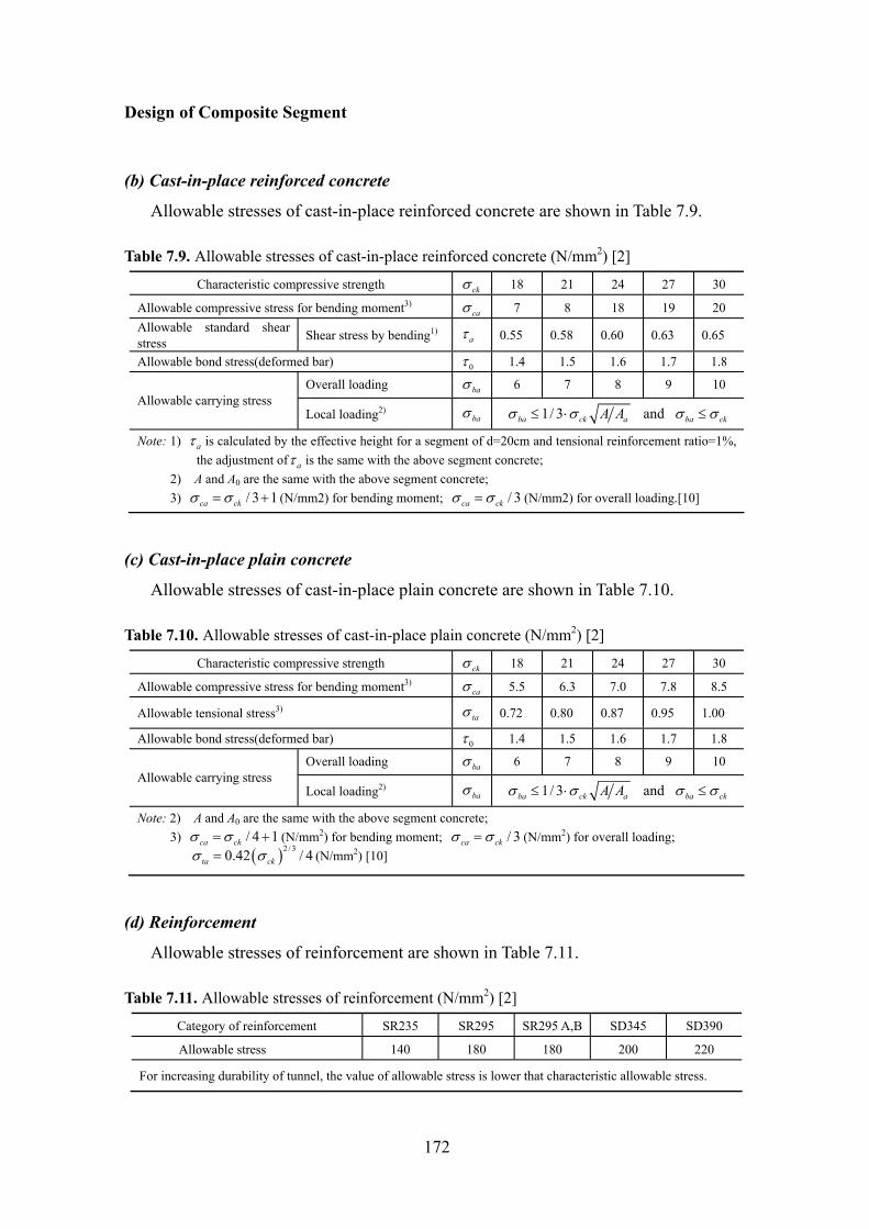
Design of Composite Segment
172
(b) Cast-in-place reinforced concrete
Allowable stresses of cast-in-place reinforced concrete are shown in Table 7.9.
Table 7.9. Allowable stresses of cast-in-place reinforced concrete (N/mm2) [2]
Characteristic compressive strength ckσ 18 21 24 27 30
Allowable compressive stress for bending moment3) caσ 7 8 18 19 20 Allowable standard shear stress Shear stress by bending1) aτ 0.55 0.58 0.60 0.63 0.65
Allowable bond stress(deformed bar) 0τ 1.4 1.5 1.6 1.7 1.8
Overall loading baσ 6 7 8 9 10 Allowable carrying stress
Local loading2) baσ 1/ 3ba ck aA Aσ σ≤ ⋅ and ba ckσ σ≤
Note: 1) aτ is calculated by the effective height for a segment of d=20cm and tensional reinforcement ratio=1%, the adjustment of aτ is the same with the above segment concrete;
2) A and A0 are the same with the above segment concrete; 3) / 3 1ca ckσ σ= + (N/mm2) for bending moment; / 3ca ckσ σ= (N/mm2) for overall loading.[10]
(c) Cast-in-place plain concrete
Allowable stresses of cast-in-place plain concrete are shown in Table 7.10.
Table 7.10. Allowable stresses of cast-in-place plain concrete (N/mm2) [2]
Characteristic compressive strength ckσ 18 21 24 27 30
Allowable compressive stress for bending moment3) caσ 5.5 6.3 7.0 7.8 8.5
Allowable tensional stress3) taσ 0.72 0.80 0.87 0.95 1.00
Allowable bond stress(deformed bar) 0τ 1.4 1.5 1.6 1.7 1.8
Overall loading baσ 6 7 8 9 10 Allowable carrying stress
Local loading2) baσ 1/ 3ba ck aA Aσ σ≤ ⋅ and ba ckσ σ≤
Note: 2) A and A0 are the same with the above segment concrete; 3) / 4 1ca ckσ σ= + (N/mm2) for bending moment; / 3ca ckσ σ= (N/mm2) for overall loading;
( )2 / 30.42 / 4ta ckσ σ= (N/mm2) [10]
(d) Reinforcement
Allowable stresses of reinforcement are shown in Table 7.11.
Table 7.11. Allowable stresses of reinforcement (N/mm2) [2]
Category of reinforcement SR235 SR295 SR295 A,B SD345 SD390
Allowable stress 140 180 180 200 220
For increasing durability of tunnel, the value of allowable stress is lower that characteristic allowable stress.
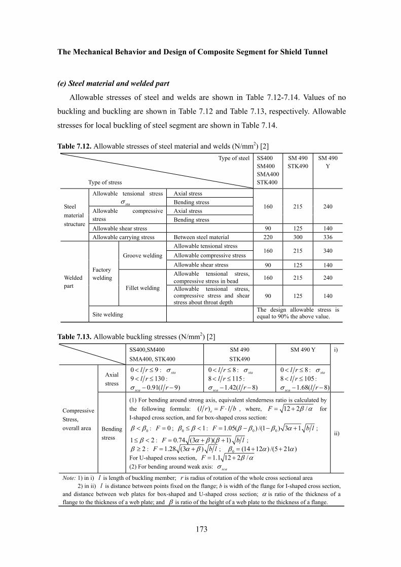
The Mechanical Behavior and Design of Composite Segment for Shield Tunnel
173
(e) Steel material and welded part
Allowable stresses of steel and welds are shown in Table 7.12-7.14. Values of no
buckling and buckling are shown in Table 7.12 and Table 7.13, respectively. Allowable
stresses for local buckling of steel segment are shown in Table 7.14.
Table 7.12. Allowable stresses of steel material and welds (N/mm2) [2] Type of steel
Type of stress
SS400 SM400 SMA400STK400
SM 490 STK490
SM 490 Y
Axial stress Allowable tensional stress staσ Bending stress
Axial stress Allowable compressive stress Bending stress
160 215 240
Allowable shear stress 90 125 140
Steel material structure
Allowable carrying stress Between steel material 220 300 336 Allowable tensional stress Allowable compressive stress
160 215 340 Groove welding
Allowable shear stress 90 125 140 Allowable tensional stress, compressive stress in bead 160 215 240
Factory welding
Fillet welding Allowable tensional stress, compressive stress and shear stress about throat depth
90 125 140
Welded part
Site welding The design allowable stress is equal to 90% the above value.
Table 7.13. Allowable buckling stresses (N/mm2) [2]
SS400,SM400 SMA400, STK400
SM 490 STK490
SM 490 Y
Axial stress
0 9l r< ≤ : staσ9 130l r< ≤ :
0.91( 9)sca l rσ − −
0 8l r< ≤ : staσ8 115l r< ≤ :
1.42( 8)sca l rσ − −
0 8l r< ≤ : staσ 8 105l r< ≤ :
1.68( 8)sca l rσ − −
i)
Compressive Stress, overall area Bending
stress
(1) For bending around strong axis, equivalent slenderness ratio is calculated by the following formula: ( )el r F l b= ⋅ , where, 12 2 /F β α= + for I-shaped cross section, and for box-shaped cross section:
0β β< : 0F = ; 0 1β β≤ < : 0 01.05( ) /(1 ) 3 1F b lβ β β α= − − + ;
1 2β≤ < : 0.74 (3 )( 1)F b lα β β= + + ; 2β ≥ : 1.28 (3 )F b lα β= + ; 0 (14 12 ) /(5 21 )β α α= + +
For U-shaped cross section, 1.1 12 2 /F β α= + (2) For bending around weak axis: scaσ
ii)
Note: 1) in i) l is length of buckling member; r is radius of rotation of the whole cross sectional area 2) in ii) l is distance between points fixed on the flange; b is width of the flange for I-shaped cross section, and distance between web plates for box-shaped and U-shaped cross section; α is ratio of the thickness of a flange to the thickness of a web plate; and β is ratio of the height of a web plate to the thickness of a flange.
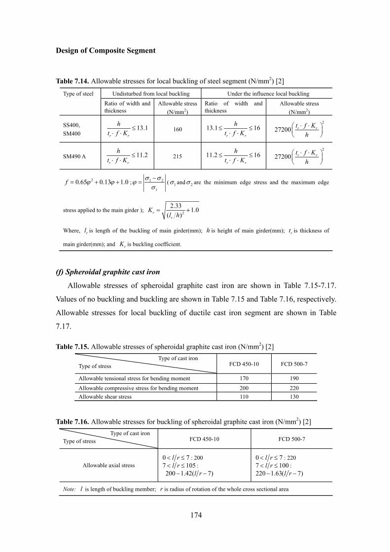
Design of Composite Segment
174
Table 7.14. Allowable stresses for local buckling of steel segment (N/mm2) [2]
Undisturbed from local buckling Under the influence local buckling Type of steel
Ratio of width and thickness
Allowable stress (N/mm2)
Ratio of width and thickness
Allowable stress (N/mm2)
SS400, SM400
13.1r r
ht f K
≤⋅ ⋅
160 13.1 16r r
ht f K
≤ ≤⋅ ⋅
2
27200 r rt f Kh
⋅ ⋅⎛ ⎞⎜ ⎟⎝ ⎠
SM490 A 11.2r r
ht f K
≤⋅ ⋅
215 11.2 16r r
ht f K
≤ ≤⋅ ⋅
2
27200 r rt f Kh
⋅ ⋅⎛ ⎞⎜ ⎟⎝ ⎠
20.65 0.13 1.0f ϕ ϕ= + + ; 1 2
1
σ σϕσ−
= ( 1σ and 2σ are the minimum edge stress and the maximum edge
stress applied to the main girder ); 2
2.33 1.0( )r
r
Kl h
= +
Where, rl is length of the buckling of main girder(mm); h is height of main girder(mm); rt is thickness of
main girder(mm); and rK is buckling coefficient.
(f) Spheroidal graphite cast iron
Allowable stresses of spheroidal graphite cast iron are shown in Table 7.15-7.17.
Values of no buckling and buckling are shown in Table 7.15 and Table 7.16, respectively.
Allowable stresses for local buckling of ductile cast iron segment are shown in Table
7.17.
Table 7.15. Allowable stresses of spheroidal graphite cast iron (N/mm2) [2] Type of cast iron Type of stress FCD 450-10 FCD 500-7
Allowable tensional stress for bending moment 170 190
Allowable compressive stress for bending moment 200 220 Allowable shear stress 110 130
Table 7.16. Allowable stresses for buckling of spheroidal graphite cast iron (N/mm2) [2] Type of cast iron Type of stress FCD 450-10 FCD 500-7
Allowable axial stress 0 7l r< ≤ : 200 7 105l r< ≤ : 200 1.42( 7)l r− −
0 7l r< ≤ : 220 7 100l r< ≤ : 220 1.63( 7)l r− −
Note: l is length of buckling member; r is radius of rotation of the whole cross sectional area
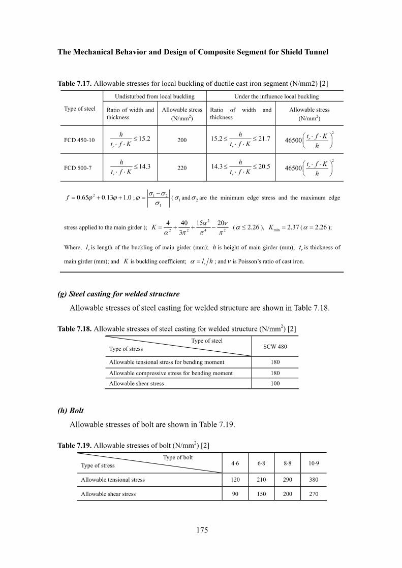
The Mechanical Behavior and Design of Composite Segment for Shield Tunnel
175
Table 7.17. Allowable stresses for local buckling of ductile cast iron segment (N/mm2) [2]
Undisturbed from local buckling Under the influence local buckling
Type of steel Ratio of width and thickness
Allowable stress (N/mm2)
Ratio of width and thickness
Allowable stress (N/mm2)
FCD 450-10 15.2r
ht f K
≤⋅ ⋅
200 15.2 21.7r
ht f K
≤ ≤⋅ ⋅
2
46500 rt f Kh
⋅ ⋅⎛ ⎞⎜ ⎟⎝ ⎠
FCD 500-7 14.3r
ht f K
≤⋅ ⋅
220 14.3 20.5r
ht f K
≤ ≤⋅ ⋅
2
46500 rt f Kh
⋅ ⋅⎛ ⎞⎜ ⎟⎝ ⎠
20.65 0.13 1.0f ϕ ϕ= + + ; 1 2
1
σ σϕσ−
= ( 1σ and 2σ are the minimum edge stress and the maximum edge
stress applied to the main girder ); 2
2 2 4 2
4 40 15 203
K α να π π π
= + + − ( 2.26α ≤ ), min 2.37K = ( 2.26α = );
Where, rl is length of the buckling of main girder (mm); h is height of main girder (mm); rt is thickness of
main girder (mm); and K is buckling coefficient; rl hα = ; andν is Poisson’s ratio of cast iron.
(g) Steel casting for welded structure
Allowable stresses of steel casting for welded structure are shown in Table 7.18.
Table 7.18. Allowable stresses of steel casting for welded structure (N/mm2) [2] Type of steel Type of stress SCW 480
Allowable tensional stress for bending moment 180
Allowable compressive stress for bending moment 180
Allowable shear stress 100
(h) Bolt
Allowable stresses of bolt are shown in Table 7.19.
Table 7.19. Allowable stresses of bolt (N/mm2) [2] Type of bolt Type of stress 4·6 6·8 8·8 10·9
Allowable tensional stress 120 210 290 380
Allowable shear stress 90 150 200 270
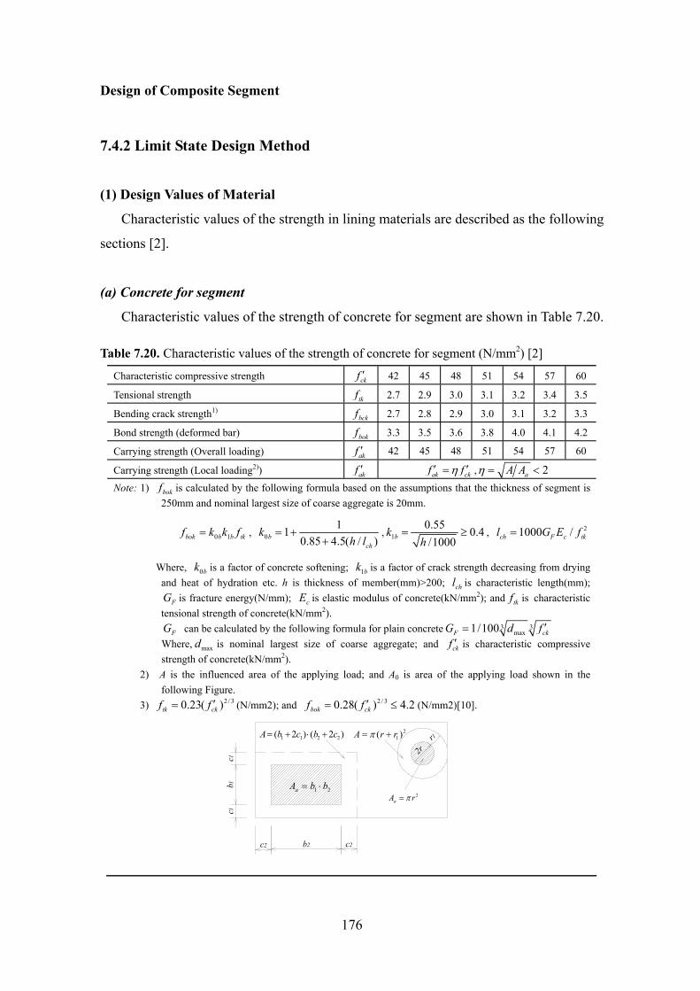
Design of Composite Segment
176
7.4.2 Limit State Design Method
(1) Design Values of Material
Characteristic values of the strength in lining materials are described as the following
sections [2].
(a) Concrete for segment
Characteristic values of the strength of concrete for segment are shown in Table 7.20.
Table 7.20. Characteristic values of the strength of concrete for segment (N/mm2) [2]
Characteristic compressive strength ckf ′ 42 45 48 51 54 57 60
Tensional strength tkf 2.7 2.9 3.0 3.1 3.2 3.4 3.5
Bending crack strength1) bckf 2.7 2.8 2.9 3.0 3.1 3.2 3.3
Bond strength (deformed bar) bokf 3.3 3.5 3.6 3.8 4.0 4.1 4.2
Carrying strength (Overall loading) akf ′ 42 45 48 51 54 57 60
Carrying strength (Local loading2)) akf ′ ak ckf fη′ ′= , 2aA Aη = <
Note: 1) bokf is calculated by the following formula based on the assumptions that the thickness of segment is 250mm and nominal largest size of coarse aggregate is 20mm.
0 1bok b b tkf k k f= , 011
0.85 4.5( / )bch
kh l
= ++
, 10.55 0.4/1000bk
h= ≥ , 21000 /ch F c tkl G E f=
Where, 0bk is a factor of concrete softening; 1bk is a factor of crack strength decreasing from drying and heat of hydration etc. h is thickness of member(mm)>200; chl is characteristic length(mm);
FG is fracture energy(N/mm); cE is elastic modulus of concrete(kN/mm2); and tkf is characteristic tensional strength of concrete(kN/mm2).
FG can be calculated by the following formula for plain concrete 3 3max1/100F ckG d f ′=
Where, maxd is nominal largest size of coarse aggregate; and ckf ′ is characteristic compressive strength of concrete(kN/mm2).
2) A is the influenced area of the applying load; and A0 is area of the applying load shown in the following Figure.
3) 2 / 30.23( )tk ckf f ′= (N/mm2); and 2 / 30.28( ) 4.2bok ckf f ′= ≤ (N/mm2)[10].
2aA rπ=
21( )A r rπ= +
1 2aA b b= ⋅
1 1 2 2( 2 ) ( 2 )A b c b c= + ⋅ +
c2 c2b2
c1b1
c1
2rr1
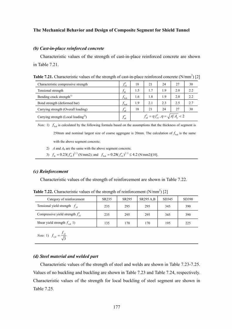
The Mechanical Behavior and Design of Composite Segment for Shield Tunnel
177
(b) Cast-in-place reinforced concrete
Characteristic values of the strength of cast-in-place reinforced concrete are shown
in Table 7.21.
Table 7.21. Characteristic values of the strength of cast-in-place reinforced concrete (N/mm2) [2]
Characteristic compressive strength ckf ′ 18 21 24 27 30
Tensional strength tkf 1.5 1.7 1.9 2.0 2.2
Bending crack strength1) bckf 1.6 1.8 1.9 2.0 2.2
Bond strength (deformed bar) bokf 1.9 2.1 2.3 2.5 2.7
Carrying strength (Overall loading) akf ′ 18 21 24 27 30
Carrying strength (Local loading2)) akf ′ ak ckf fη′ ′= , 2aA Aη = <
Note: 1) bokf is calculated by the following formula based on the assumptions that the thickness of segment is
250mm and nominal largest size of coarse aggregate is 20mm. The calculation of bokf is the same
with the above segment concrete;
2) A and A0 are the same with the above segment concrete;
3) 2 / 30.23( )tk ckf f ′= (N/mm2); and 2 / 30.28( ) 4.2bok ckf f ′= ≤ (N/mm2)[10].
(c) Reinforcement
Characteristic values of the strength of reinforcement are shown in Table 7.22.
Table 7.22. Characteristic values of the strength of reinforcement (N/mm2) [2]
Category of reinforcement SR235 SR295 SR295 A,B SD345 SD390
Tensional yield strength ykf 235 295 295 345 390
Compressive yield strength ykf ′ 235 295 295 345 390
Shear yield strength vykf 1) 135 170 170 195 225
Note: 1) 3yk
vyk
ff =
(d) Steel material and welded part
Characteristic values of the strength of steel and welds are shown in Table 7.23-7.25.
Values of no buckling and buckling are shown in Table 7.23 and Table 7.24, respectively.
Characteristic values of the strength for local buckling of steel segment are shown in
Table 7.25.

Design of Composite Segment
178
Table 7.23. Characteristic values of the strength of steel material and welds (N/mm2) [2] Type of steel
Type of stress
SS400 SM400 SMA400STK400
SM 490
STK490
SM 490Y SMA490 SM 520
SM570SMA570
Tensional yield strength ykf 235 315 355 450
Compressive yield strength ykf ′ 235 315 355 450
Shear yield strength vykf
(overall area) 135 180 205 260 Steel material structure
Carrying strength akf ′ (between
steel material) 350 470 530 675
Tensional yield strength ykf
Compressive yield strength ykf ′235 315 355 450
Groove welding
Shear yield strength vykf
(overall area) 135 180 205 260
Tensional and compressive yield strength in bead 235 315 355 450
Factory welding
Fillet welding Tensional , compressive and
shear yield strength about throat depth
135 180 205 260
Welded part
Site welding The design allowable stress is equal to 90% the above value.
Table 7.24. Characteristic values of steel buckling (N/mm2) [2]
SS400,SM400 SMA400, STK400
SM 490 STK490
SM 490Y SMA490SM 520
SM570 SMA570
Axial strength
0 9l r< ≤ : ykf ′ 9 130l r< ≤ :
1.33( 9)ykf l r′ − −
0 8l r< ≤ : ykf ′ 8 115l r< ≤ :
2.06( 8)ykf l r′ − −
0 8l r< ≤ : ykf ′ 8 105l r< ≤ :
2.46( 8)ykf l r′ − −
0 7l r< ≤ : ykf ′ 7 95l r< ≤ :
3.51( 7)ykf l r′ − −
i)
Com
pres
sive
yie
ld S
treng
th O
vera
ll ar
ea
Bending strength
(1) For bending around strong axis, equivalent slenderness ratio is calculated by the following formula: ( )el r F l b= ⋅ , where, 12 2 /F β α= + for I-shaped cross section, and for box-shaped cross section:
0β β< : 0F = ; 0 1β β≤ < : 0 01.05( ) /(1 ) 3 1F b lβ β β α= − − + ;
1 2β≤ < : 0.74 (3 )( 1)F b lα β β= + + ; 2β ≥ : 1.28 (3 )F b lα β= + ; 0 (14 12 ) /(5 21 )β α α= + +
For U-shaped cross section, 1.1 12 2 /F β α= +
(2) For bending around weak axis: ykf ′
ii)
Note: 1) in i) l is length of buckling member; r is radius of rotation of the whole cross sectional area 2) in ii) l is distance between points fixed on the flange; b is width of the flange for I-shaped cross section, and distance between web plates for box-shaped and U-shaped cross section; α is ratio of the thickness of a flange to the thickness of a web plate; and β is ratio of the height of a web plate to the thickness of a flange.
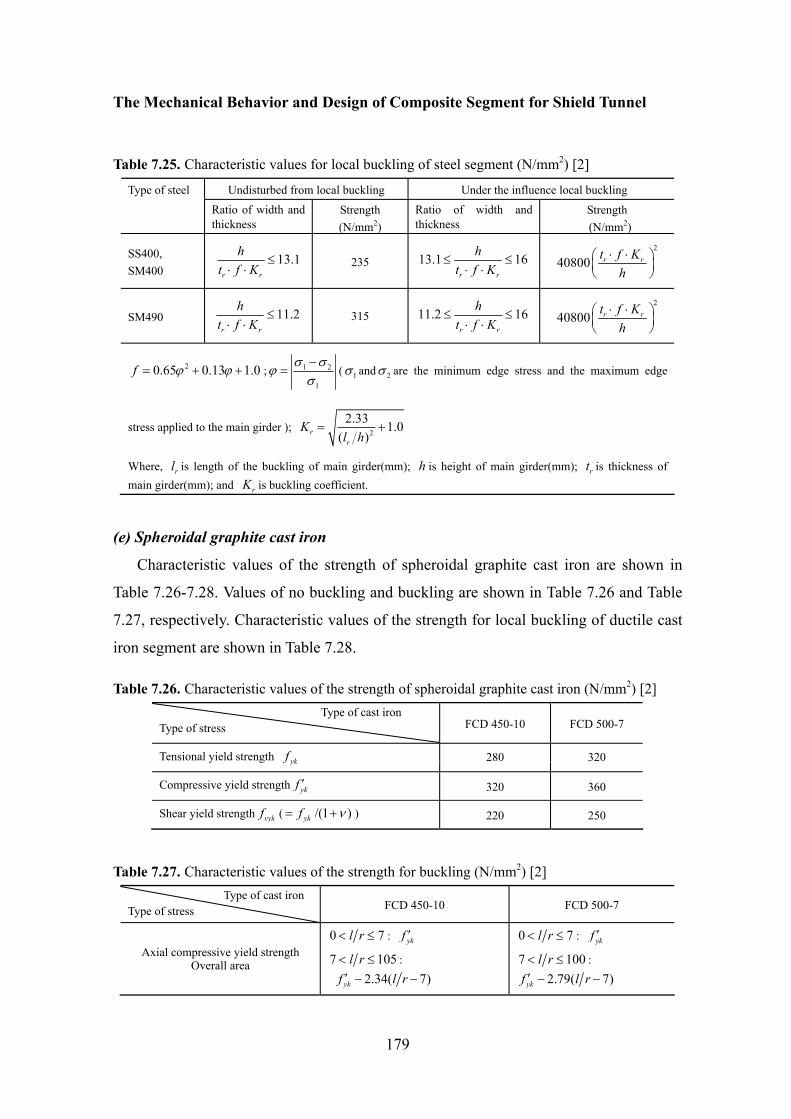
The Mechanical Behavior and Design of Composite Segment for Shield Tunnel
179
Table 7.25. Characteristic values for local buckling of steel segment (N/mm2) [2]
Undisturbed from local buckling Under the influence local buckling Type of steel
Ratio of width and thickness
Strength (N/mm2)
Ratio of width and thickness
Strength (N/mm2)
SS400, SM400
13.1r r
ht f K
≤⋅ ⋅
235 13.1 16r r
ht f K
≤ ≤⋅ ⋅
2
40800 r rt f Kh
⋅ ⋅⎛ ⎞⎜ ⎟⎝ ⎠
SM490 11.2r r
ht f K
≤⋅ ⋅
315 11.2 16r r
ht f K
≤ ≤⋅ ⋅
2
40800 r rt f Kh
⋅ ⋅⎛ ⎞⎜ ⎟⎝ ⎠
20.65 0.13 1.0f ϕ ϕ= + + ; 1 2
1
σ σϕσ−
= ( 1σ and 2σ are the minimum edge stress and the maximum edge
stress applied to the main girder ); 2
2.33 1.0( )r
r
Kl h
= +
Where, rl is length of the buckling of main girder(mm); h is height of main girder(mm); rt is thickness of main girder(mm); and rK is buckling coefficient.
(e) Spheroidal graphite cast iron
Characteristic values of the strength of spheroidal graphite cast iron are shown in
Table 7.26-7.28. Values of no buckling and buckling are shown in Table 7.26 and Table
7.27, respectively. Characteristic values of the strength for local buckling of ductile cast
iron segment are shown in Table 7.28.
Table 7.26. Characteristic values of the strength of spheroidal graphite cast iron (N/mm2) [2] Type of cast iron Type of stress FCD 450-10 FCD 500-7
Tensional yield strength ykf 280 320
Compressive yield strength ykf ′ 320 360
Shear yield strength vykf ( /(1 )ykf ν= + ) 220 250
Table 7.27. Characteristic values of the strength for buckling (N/mm2) [2] Type of cast iron Type of stress FCD 450-10 FCD 500-7
Axial compressive yield strength Overall area
0 7l r< ≤ : ykf ′
7 105l r< ≤ : 2.34( 7)ykf l r′ − −
0 7l r< ≤ : ykf ′
7 100l r< ≤ : 2.79( 7)ykf l r′ − −
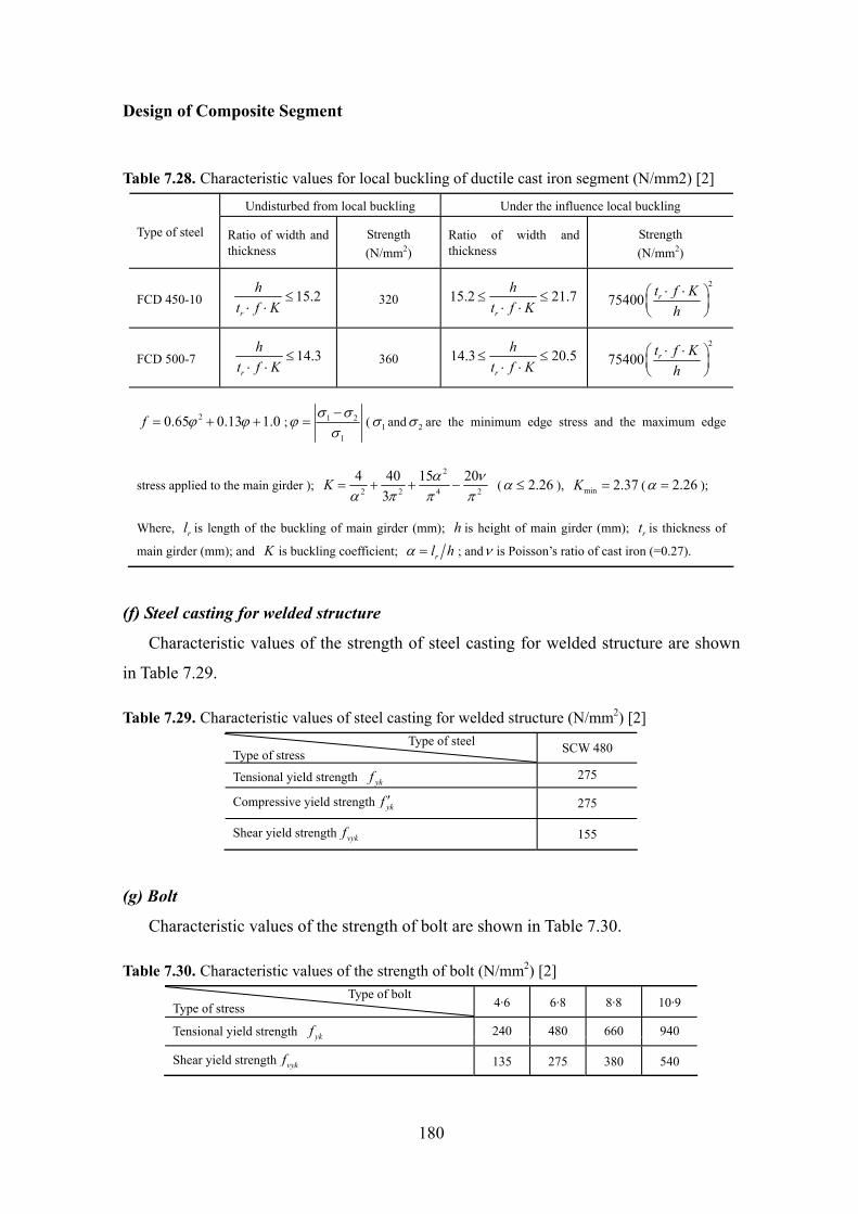
Design of Composite Segment
180
Table 7.28. Characteristic values for local buckling of ductile cast iron segment (N/mm2) [2]
Undisturbed from local buckling Under the influence local buckling
Type of steel Ratio of width and thickness
Strength (N/mm2)
Ratio of width and thickness
Strength (N/mm2)
FCD 450-10 15.2r
ht f K
≤⋅ ⋅
320 15.2 21.7r
ht f K
≤ ≤⋅ ⋅
2
75400 rt f Kh
⋅ ⋅⎛ ⎞⎜ ⎟⎝ ⎠
FCD 500-7 14.3r
ht f K
≤⋅ ⋅
360 14.3 20.5r
ht f K
≤ ≤⋅ ⋅
2
75400 rt f Kh
⋅ ⋅⎛ ⎞⎜ ⎟⎝ ⎠
20.65 0.13 1.0f ϕ ϕ= + + ; 1 2
1
σ σϕσ−
= ( 1σ and 2σ are the minimum edge stress and the maximum edge
stress applied to the main girder ); 2
2 2 4 2
4 40 15 203
K α να π π π
= + + − ( 2.26α ≤ ), min 2.37K = ( 2.26α = );
Where, rl is length of the buckling of main girder (mm); h is height of main girder (mm); rt is thickness of
main girder (mm); and K is buckling coefficient; rl hα = ; andν is Poisson’s ratio of cast iron (=0.27).
(f) Steel casting for welded structure
Characteristic values of the strength of steel casting for welded structure are shown
in Table 7.29.
Table 7.29. Characteristic values of steel casting for welded structure (N/mm2) [2] Type of steel Type of stress SCW 480
Tensional yield strength ykf 275
Compressive yield strength ykf ′ 275
Shear yield strength vykf 155
(g) Bolt
Characteristic values of the strength of bolt are shown in Table 7.30.
Table 7.30. Characteristic values of the strength of bolt (N/mm2) [2] Type of bolt Type of stress 4·6 6·8 8·8 10·9
Tensional yield strength ykf 240 480 660 940
Shear yield strength vykf 135 275 380 540

The Mechanical Behavior and Design of Composite Segment for Shield Tunnel
181
(2) Stress-Strain Curve of Material
Stress-strain curves of material must be determined in limit state. Fig.7.9 shows the
stress-strain curves of concrete, steel, reinforcement, spheroidal graphite cast iron, and
bolt, which are used in limit state for considering failure of the cross-section in
“Standard specifications for tunneling-2006, Shield tunnels” in Japan [2].
1 cdk f ′
0
: Compressive strength of concrete(N/mm2)
0.002 cuε ′
ckf ′
1 1 0.003 0.85ckk f ′= − ≤
0.0025 0.0035cuε′≤ ≤
15530000
ckcu
fε′−′ =cσ
1 20.002 0.002
c cc ckk f ε εσ ⎛ ⎞′= −⎜ ⎟
⎝ ⎠
0
ydfydf
s ydfσ =
s sEσ ε=sσ
: Tensional yield strength (N/mm2)
ε (a) Concrete (b) Steel, reinforcement, spheroidal graphite cast iron, bolt
Fig.7.9 Stress-strain curve
Linear stress-strain curves of material are used in the serviceability limit state. The
elastic moduli of materials are shown in Table 7.31 and Table 7.32.
Table 7.31. Elastic modulus of concrete (segment) [2]
Characteristic compressive strength ckf ′ (N/mm2) 42 45 48 51 54 57 60
Elastic modulus cE (kN/mm2) 31.4 32.0 32.6 33.2 33.8 34.4 25.0
Table 7.32. Elastic modulus of steel, reinforcement, and spheroidal graphite cast iron [2]
Type of material Elastic modulus(kN/mm2)
Steel and steel casting sE 210
Spheroidal graphite cast iron dE 170
Poisson’s ratio of concert, steel, steel casting, and spheroidal graphite cast iron is
shown in Table 7.33
Table 7.33. Poisson’s ratio [2] Material Poisson’s ratio
Elastic range 0.17 Concrete Cracks occurred 0
Steel and steel casting 0.30 Spheroidal graphite cast iron 0.27

Design of Composite Segment
182
(3) Safety Factor
It should address safety factors in the limit state design method. These are as
follows: 1) Material factor mγ
2) Member factor bγ
3) Load factor fγ
4) Structural analysis factor aγ
5) Structure factor iγ
(a) Material factor
Material factor is shown in Table 7.34.
Table 7.34. Nominal standard for material factor [2]
Material factor mγ
Concrete Steel material Limit state
Segment Cast-in place
Reinforcement bar Main girder
Longitudinal ribSkin plate
Spheroidal graphite cast iron
Bolt
Ultimate limit state 1.2 1.3 1.00 1.05 1.00 1.10 1.05Serviceability limit state 1.0 1.0 1.00 1.00 1.00 1.00 1.00
(b) Member factor
Member factor is shown in Table 7.35 and Table 7.36.
Table 7.35. Nominal standard for member factor (Concrete segment) [2]
Member factor bγ
Main part Limit state
Bending Compression Shear
Circumferential joint
Longitudinal joint
Metallic fitting for hanging
Ultimate limit state 1.10 1.30 1.301)
1.102) 1.10 1.15 1.30
Serviceability limit state 1.0 1.0 1.00 1.00 1.00 1.00
Note: 1) The calculation of shear capacity obtained by the strength of concrete.
2) The calculation of shear capacity obtained by the strength of steel.
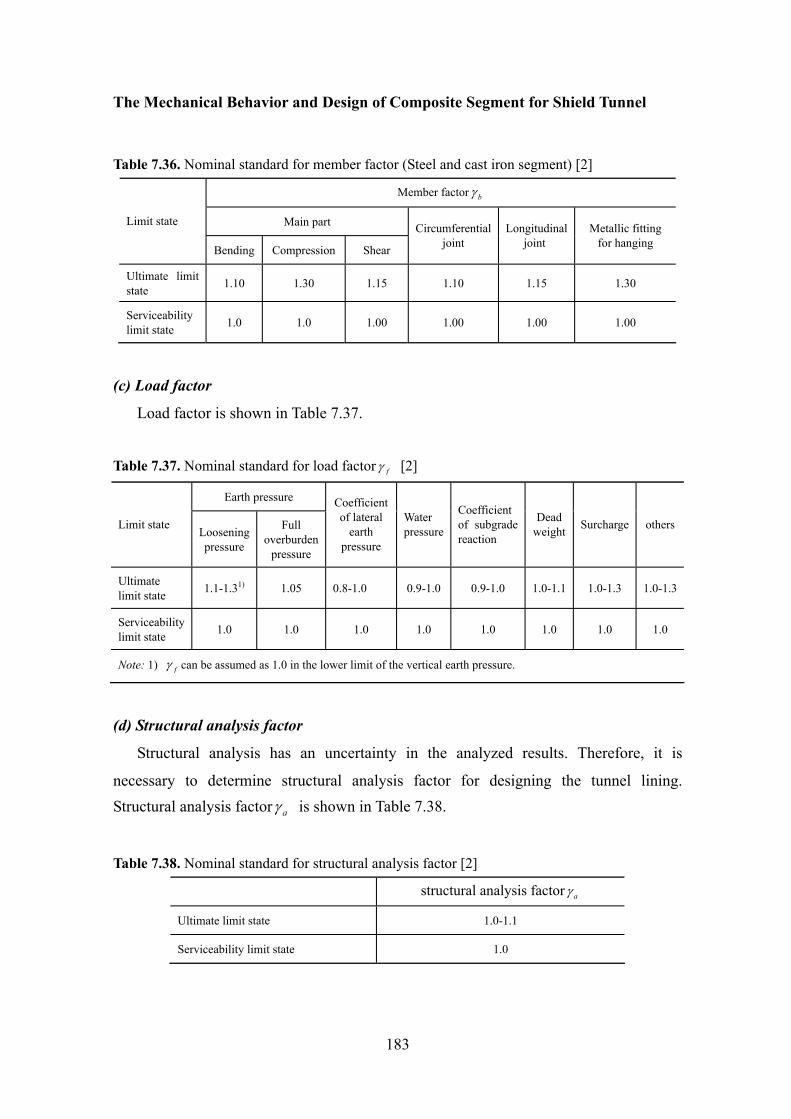
The Mechanical Behavior and Design of Composite Segment for Shield Tunnel
183
Table 7.36. Nominal standard for member factor (Steel and cast iron segment) [2]
Member factor bγ
Main part Limit state
Bending Compression Shear
Circumferential joint
Longitudinal joint
Metallic fitting for hanging
Ultimate limit state 1.10 1.30 1.15 1.10 1.15 1.30
Serviceability limit state 1.0 1.0 1.00 1.00 1.00 1.00
(c) Load factor
Load factor is shown in Table 7.37.
Table 7.37. Nominal standard for load factor fγ [2]
Earth pressure
Limit state Loosening pressure
Full overburden
pressure
Coefficient of lateral
earth pressure
Water pressure
Coefficient of subgrade reaction
Dead weight Surcharge others
Ultimate limit state 1.1-1.31) 1.05 0.8-1.0 0.9-1.0 0.9-1.0 1.0-1.1 1.0-1.3 1.0-1.3
Serviceability limit state 1.0 1.0 1.0 1.0 1.0 1.0 1.0 1.0
Note: 1) fγ can be assumed as 1.0 in the lower limit of the vertical earth pressure.
(d) Structural analysis factor
Structural analysis has an uncertainty in the analyzed results. Therefore, it is
necessary to determine structural analysis factor for designing the tunnel lining. Structural analysis factor aγ is shown in Table 7.38.
Table 7.38. Nominal standard for structural analysis factor [2]
structural analysis factor aγ
Ultimate limit state 1.0-1.1
Serviceability limit state 1.0
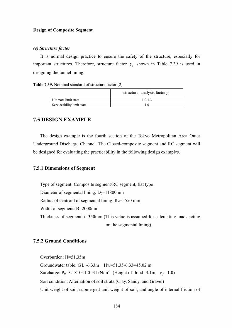
Design of Composite Segment
184
(e) Structure factor
It is normal design practice to ensure the safety of the structure, especially for important structures. Therefore, structure factor sγ shown in Table 7.39 is used in
designing the tunnel lining.
Table 7.39. Nominal standard of structure factor [2]
structural analysis factor sγ
Ultimate limit state 1.0-1.3 Serviceability limit state 1.0
7.5 DESIGN EXAMPLE
The design example is the fourth section of the Tokyo Metropolitan Area Outer
Underground Discharge Channel. The Closed-composite segment and RC segment will
be designed for evaluating the practicability in the following design examples.
7.5.1 Dimensions of Segment
Type of segment: Composite segment/RC segment, flat type
Diameter of segmental lining: D0=11800mm
Radius of centroid of segmental lining: Rc=5550 mm
Width of segment: B=2000mm
Thickness of segment: t=350mm (This value is assumed for calculating loads acting
on the segmental lining)
7.5.2 Ground Conditions
Overburden: H=51.35m
Groundwater table: G.L.-6.33m Hw=51.35-6.33=45.02 m Surcharge: P0=3.1×10×1.0=31kN/m2 (Height of flood=3.1m; fγ =1.0)
Soil condition: Alternation of soil strata (Clay, Sandy, and Gravel)
Unit weight of soil, submerged unit weight of soil, and angle of internal friction of

The Mechanical Behavior and Design of Composite Segment for Shield Tunnel
185
soil, and N value are shown in Fig.7.10.
N=6.0C=25 kN/m3
C=6.3 kN/m3
N=2.9
N=6.0
N=22.9C=120 kN/m3
C=0 kN/m3
N=39C=0 kN/m3
φ=0 degree
φ=40 degree
φ=0 degree
φ=0 degree
38.0kN/mγ ′ =
318.0kN/mγ =
39.6kN/mγ′=
319.6kN/mγ =
39.6kN/mγ′=
319.6kN/mγ =
35.3kN/mγ ′ =
315.3kN/mγ =
37.4kN/mγ′ =
317.4kN/mγ =
6.55
m25
.1m
9.1m
3.7m
11.8
m51
.35m
-44.75m
-6.33m Ground water Table
+6.60m
+9.70m Flood water Table
Clay in alluvial (Ac1)
Clay in alluvial (Ac2)
Sand in alluvial (Ns1)
Gravel in alluvial (Ng1)
Clay in diluvial (Dc2)
Clay in diluvial (Dc3)
Sand in diluvial (Ds3)
φ=0 degree
Fig.7.10 Ground condition
7.5.3 Load Conditions
The forces applying on tunnel lining are calculated based on combined load case
shown in Table 7.40.
Table 7.40. Combined load case Earth pressure Groundwater table Inner water pressure Load
case Tunnel
condition Large small High Low Normal Abnormal
Self weight
Subgrade reaction
1 No inner water pressure × × × ×
2 No inner water pressure × × × ×
3 Normal inner water pressure × × × × ×
4 Normal inner water pressure × × × × ×
5 Abnormal inner water pressure × × × × ×
6 Abnormal inner water pressure × × × × ×

Design of Composite Segment
186
The vertical earth pressure at the tunnel crown ( 1ep ) is calculated by Terzahgi’s
formula based on flow chart of calculation of the loads shown in Fig.7.2. The tunnel is
located in alternation of soil strata, and main stratum is hard clayey of soil stratum.
Therefore, earth pressure calculate is calculated using Soil-Water integrated method.
Vertical pressure at tunnel crown: Earth pressure: 2
1 468.2kN / me f vp γ σ= =
21 1 468.2kN / mv ep p= =
Lateral pressure at tunnel crown: Earth pressure: ( ) 2
1 0.5 211.9kN / me f c v iq tγ λ σ γ= + =
21 1 211.9kN / mh eq q= =
Lateral pressure at tunnel bottom:
Earth pressure: ( ){ } 22 0 0.5 265.4kN / me f c v iq D tγ λ σ γ= + − =
22 2 265.4kN / mh eq q= =
7.5.4 Calculation of Member Forces
The member forces are calculated by Shell-Spring model shown in Fig.7.11. The
segments are assembled in a staggered pattern.
Anchor joint (AS) joint and axial slide (Fig.7.12) were used as circumferential joint,
and longitudinal joint respectively, in Tokyo Metropolitan Area Outer Underground
Discharge Channel. These constants of springs were obtained by the experiments, and
described as follows:
Constants of spring of circumferential joint:
Axial spring: 65.0 10 kN / mc
ak = ×
Shear spring: 52.2 10 kN / mc
sk = ×
Rotational spring: 5
5
1.77 10 kNm/rad (Positive bending)1.67 10 kNm/rad (Negative bending)
ckθ⎧ ×
= ⎨×⎩
Constants of spring of longitudinal joint:
Axial spring: 64.8 10 kN / mL
ak = ×
Shear spring: 52.1 10 kN / mL
sk = × Rotational spring: 42.2 10 kN / mLkθ = ×
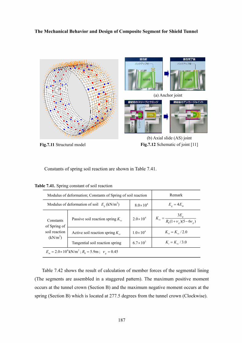
The Mechanical Behavior and Design of Composite Segment for Shield Tunnel
187
Constants of spring soil reaction are shown in Table 7.41.
Table 7.41. Spring constant of soil reaction
Modulus of deformation; Constants of Spring of soil reaction Remark
Modulus of deformation of soil gE (kN/m2) 48.0 10× 4g mE E=
Passive soil reaction spring rcK 42.0 10× 0
3(1 )(5 6 )
grc
g g
EK
R ν ν=
+ −
Active soil reaction spring rtK 41.0 10× / 2.0rt rcK K=
Constants of Spring of soil reaction
(kN/m2) Tangential soil reaction spring 36.7 10× / 3.0t rcK K=
4 22.0 10 kN/mmE = × ; 0 5.9mR = ; 0.45gν =
Table 7.42 shows the result of calculation of member forces of the segmental lining
(The segments are assembled in a staggered pattern). The maximum positive moment
occurs at the tunnel crown (Section B) and the maximum negative moment occurs at the
spring (Section B) which is located at 277.5 degrees from the tunnel crown (Clockwise).
Fig.7.11 Structural model
(a) Anchor joint
(b) Axial slide (AS) joint Fig.7.12 Schematic of joint [11]

Design of Composite Segment
188
Table 7.42. Member forces of segmental lining (A-Ring)
θ (deg)
Bending moment M
(kN m/Ring)⋅
Axial force N
(kN/Ring)
Shear forceQ
(kN/Ring)θ
(deg) Bending moment
M (kN m/Ring)⋅
Axial force N
(kN/Ring)
Shear forceQ
(kN/Ring)
0.0 606.1 3485.9 -90.0 101.3 -450.7 4714.8 -24.1
3.8 635.5 3487.9 -28.9 105.0 -439.8 4677.3 -70.6
7.5 628.5 3487.7 32.7 108.8 -396.2 4639.1 -116.5
11.3 610.4 3512.9 62.5 112.5 -349.9 4590.3 -122.8
15.0 580.2 3560.0 139.7 116.3 -301.5 4527.5 -135.2
18.8 502.6 3608.1 212.4 120.0 -245.6 4466.5 -152.3
22.5 416.3 3671.7 232.3 123.8 -184.0 4397.4 -159.6
26.3 323.4 3751.8 252.7 127.5 -130.1 4334.3 -141.4
30.0 221.3 3832.9 269.5 131.3 -75.0 4267.2 -147.5
33.8 115.5 3918.9 274.3 135.0 -16.3 4200.8 -157.5
37.5 16.7 4004.0 244.0 138.8 46.5 4134.1 -157.2
41.3 -72.7 4095.1 223.4 142.5 104.9 4069.6 -150.9
45.0 -155.6 4179.5 204.6 146.3 162.8 4008.7 -149.4
48.8 -230.5 4259.8 164.4 150.0 220.1 3954.6 -132.1
52.5 -282.4 4342.3 124.3 153.8 264.7 3903.7 -110.5
56.3 -326.4 4413.8 106.3 157.5 305.3 3857.7 -102.2
60.0 -364.3 4472.8 65.8 161.3 343.4 3820.0 -100.1
63.8 -377.0 4532.8 26.8 165.0 382.5 3784.3 -83.3
67.5 -384.9 4582.5 18.0 168.8 407.6 3753.3 -65.2
71.3 -390.8 4618.9 15.0 172.5 450.9 3729.1 -108.2
75.0 -396.4 4657.3 2.4 176.3 491.2 3703.2 -96.0
78.8 -392.6 4689.9 -9.8 180.0 525.0 3691.8 -77.3
82.5 -410.3 4708.2 47.1 183.8 550.9 3690.4 -27.7
86.3 -429.0 4732.0 47.8 187.5 546.4 3688.8 22.5
90.0 -447.2 4740.4 45.0 191.3 533.6 3707.4 45.5
93.8 -463.7 4738.1 14.3 195.0 511.4 3744.0 110.6
97.5 -458.3 4735.5 -17.0 198.8 448.2 3781.0 172.8
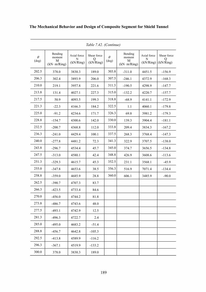
The Mechanical Behavior and Design of Composite Segment for Shield Tunnel
189
Table 7.42. (Continue)
θ (deg)
Bending moment
M (kN m/Ring)⋅
Axial force N
(kN/Ring)
Shear forceQ
(kN/Ring)θ
(deg)
Bending moment
M (kN m/Ring)⋅
Axial force N
(kN/Ring)
Shear forceQ
(kN/Ring)
202.5 378.0 3830.3 189.0 303.8 -311.0 4451.5 -156.9
206.3 302.4 3893.9 206.0 307.5 -246.1 4372.9 -168.3
210.0 219.1 3957.8 221.6 311.3 -190.5 4298.9 -147.7
213.8 131.4 4027.1 227.3 315.0 -132.2 4220.7 -157.7
217.5 50.9 4093.5 199.3 318.8 -68.9 4141.1 -172.9
221.3 -22.3 4166.3 184.2 322.5 1.1 4060.1 -179.8
225.0 -91.2 4234.6 171.7 326.3 69.8 3981.2 -179.3
228.8 -154.7 4300.6 142.0 330.0 139.3 3904.4 -181.1
232.5 -200.7 4368.8 112.0 333.8 209.4 3834.3 -167.2
236.3 -241.0 4429.4 100.1 337.5 268.3 3768.4 -147.3
240.0 -277.8 4481.2 72.3 341.3 322.9 3707.5 -138.0
243.8 -296.7 4534.4 45.7 345.0 374.7 3656.5 -134.8
247.5 -313.0 4580.1 42.4 348.8 426.9 3608.6 -113.6
251.3 -329.3 4615.7 45.3 352.5 231.1 3568.1 -45.9
255.0 -347.8 4653.6 38.5 356.3 516.9 7071.4 -134.4
258.8 -359.0 4685.9 28.8 360.0 606.1 3485.9 -90.0
262.5 -390.7 4707.3 83.7
266.3 -423.5 4733.4 84.6
270.0 -456.0 4744.2 81.8
273.8 -486.7 4743.6 48.0
277.5 -493.1 4742.9 12.5
281.3 -496.3 4722.7 2.4
285.0 -495.0 4683.2 -51.4
288.8 -456.7 4642.8 -105.3
292.5 -413.8 4589.9 -116.2
296.3 -367.1 4519.9 -133.2
300.0 378.0 3830.3 189.0
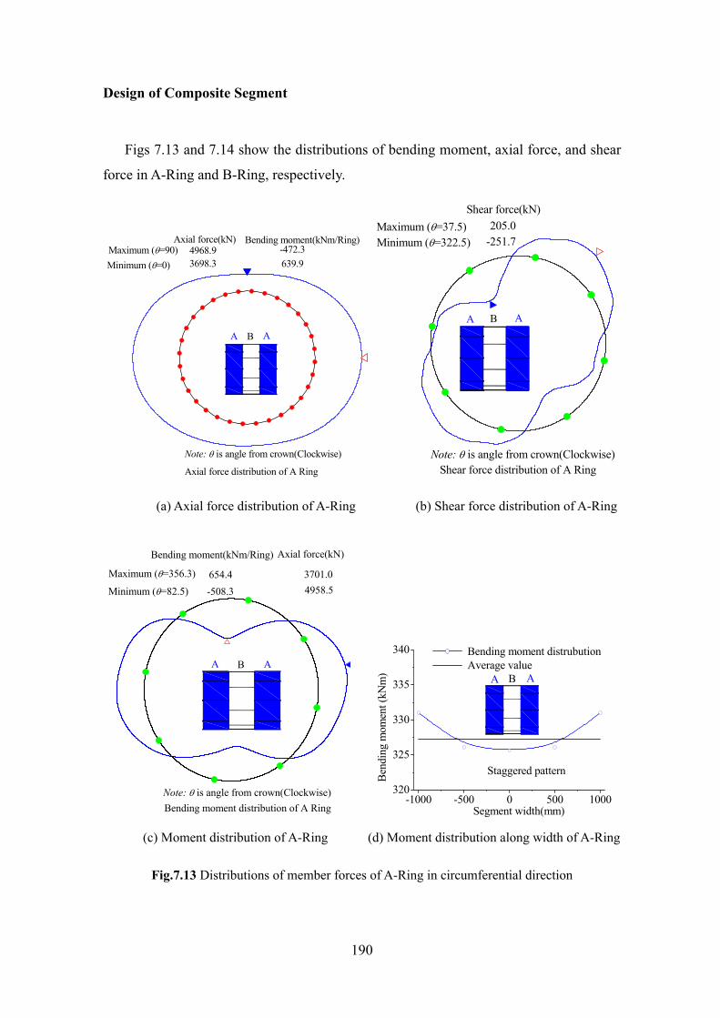
Design of Composite Segment
190
Figs 7.13 and 7.14 show the distributions of bending moment, axial force, and shear
force in A-Ring and B-Ring, respectively.
639.9-472.3
3698.34968.9
Note: θ is angle from crown(Clockwise)
Axial force distribution of A Ring
ABA
Minimum (θ=0)
Bending moment(kNm/Ring)Axial force(kN)Maximum (θ=90)
Note: θ is angle from crown(Clockwise)Shear force distribution of A Ring
ABA
-251.7205.0
Minimum (θ=322.5)
Shear force(kN)Maximum (θ=37.5)
(a) Axial force distribution of A-Ring (b) Shear force distribution of A-Ring
Note: θ is angle from crown(Clockwise)
4958.53701.0
Axial force(kN)
Bending moment distribution of A Ring
ABA
-508.3654.4
Minimum (θ=82.5)
Bending moment(kNm/Ring)
Maximum (θ=356.3)
-1000 -500 0 500 1000
320
325
330
335
340
Staggered pattern
Bending moment distrubution Average value
B AA
Segment width(mm)
Bend
ing
mom
ent (
kNm
)
(c) Moment distribution of A-Ring (d) Moment distribution along width of A-Ring
Fig.7.13 Distributions of member forces of A-Ring in circumferential direction
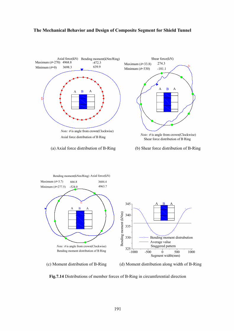
The Mechanical Behavior and Design of Composite Segment for Shield Tunnel
191
3698.34968.8
Note: θ is angle from crown(Clockwise)
Axial force distribution of B Ring
ABA
639.9-472.3
Minimum (θ=0)
Bending moment(kNm/Ring)Axial force(kN)Maximum (θ=270)
-181.1274.3
A
Note: θ is angle from crown(Clockwise)Shear force distribution of B Ring
BA
Minimum (θ=330)
Shear force(kN)Maximum (θ=33.8)
(a) Axial force distribution of B-Ring (b) Shear force distribution of B-Ring
Note: θ is angle from crown(Clockwise)
4963.73684.4
Axial force(kN)
Bending moment distribution of B Ring
ABA
-524.0666.8
Minimum (θ=277.5)
Bending moment(kNm/Ring)
Maximum (θ=3.7)
-1000 -500 0 500 1000
325
330
335
340
345
Staggered pattern
Bending moment distrubution Average value
B AA
Segment width(mm)
Ben
ding
mom
ent (
kNm
)
(c) Moment distribution of B-Ring (d) Moment distribution along width of B-Ring
Fig.7.14 Distributions of member forces of B-Ring in circumferential direction
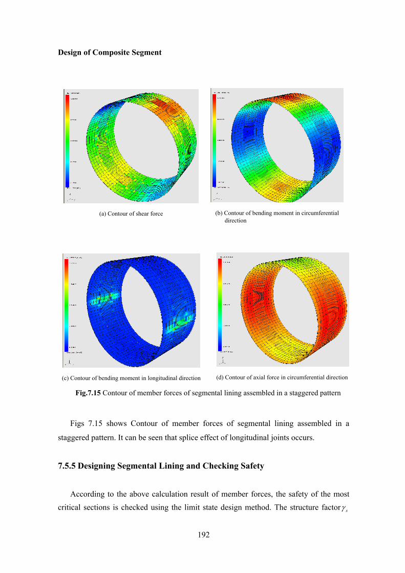
Design of Composite Segment
192
(c) Contour of bending moment in longitudinal direction
(a) Contour of shear force
Figs 7.15 shows Contour of member forces of segmental lining assembled in a
staggered pattern. It can be seen that splice effect of longitudinal joints occurs.
7.5.5 Designing Segmental Lining and Checking Safety
According to the above calculation result of member forces, the safety of the most critical sections is checked using the limit state design method. The structure factor sγ
(b) Contour of bending moment in circumferential direction
(d) Contour of axial force in circumferential direction
Fig.7.15 Contour of member forces of segmental lining assembled in a staggered pattern
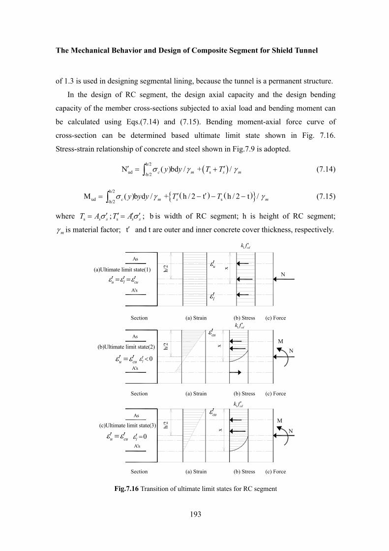
The Mechanical Behavior and Design of Composite Segment for Shield Tunnel
193
of 1.3 is used in designing segmental lining, because the tunnel is a permanent structure.
In the design of RC segment, the design axial capacity and the design bending
capacity of the member cross-sections subjected to axial load and bending moment can
be calculated using Eqs.(7.14) and (7.15). Bending moment-axial force curve of
cross-section can be determined based ultimate limit state shown in Fig. 7.16.
Stress-strain relationship of concrete and steel shown in Fig.7.9 is adopted.
( )h/2
ud s-h/2N ( )bd / + / c m s my y T Tσ γ γ′ ′= +∫ (7.14)
( ) ( ){ }h/2
ud s-h/2 M ( )b d / + h / 2 t h / 2 t / c m s my y y T Tσ γ γ′ ′= − − −∫ (7.15)
where s s sT Aσ ′= ; s s sT Aσ′ ′ ′= ; b is width of RC segment; h is height of RC segment;
mγ is material factor; t′ and t are outer and inner concrete cover thickness, respectively.
0lε′<
0lε′ =u cuε ε′ ′=(c)Ultimate limit state(3)
(b)Ultimate limit state(2)
u cuε ε′ ′=
u l cuε ε ε′ ′ ′= =
cuε′
cuε′
lε′
uε′
M
N
N
1 cdk f ′
1 cdk f ′
A's
As
As
A's
h/2 x
h/2 x
h/2
x
(a) Strain (b) Stress (c) Force
(a) Strain (b) Stress (c) Force
(a) Strain (b) Stress (c) Force
Section
Section
Section
(a)Ultimate limit state(1)
MN
1 cdk f ′
A's
As
Fig.7.16 Transition of ultimate limit states for RC segment

Design of Composite Segment
194
2sA 6193.6 mm=
2sA 6193.6 mm′ =
Strength of concrete: 48N/mm2
350
2000
7565
D22 16@120
Unit: mm
D22 (SD345)
D22 (SD345)
D22 16@120
Fig.7.17 Section of RC segment and arrangement of main reinforcements
0 200 400 600 800 1000 12000
2000
4000
6000
8000
10000
12000
14000
16000
18000
20000 Maximum positive moment Maximum negative moment
Axi
al fo
rce
(kN
)
Bending moment (kNm)
Fig.7.18 Axial force-moment interaction diagram of RC segment
Fig.7.17 shows the design cross-section of RC segment. Axial force-moment
interaction diagram of cross-section is described by Fig.7.18. Therefore, as a rule, the
safety for combined axial load and bending moment is examined by confirming that the
point (Md, Nd) is located inside of the (Mud, N'ud) curve. It can be seen that both Section
A and Section B are safe.
The Mechanical Behavior and Design of Composite Segment for Shield Tunnel
195
In the design of composite segment, the following design rules must be ensured.
(a) Width to Thickness Ratio
Elastic buckling stress for a rectangular plate subjected to an axial compression can
be calculated using Eq. (7.16), where ν is a Poisson’s ratio (0.3 for steel), and k is a
bucking coefficient that is determined from boundary conditions and aspect ratios of the
plate. When the plate is sufficiently long, the coefficient k depends only on the boundary
conditions. The values of k are given as 4.0, 5.42, and 6.97 for both edges simply
supported, one edge simply supported with the other fixed, and both edges fixed, respectively [12]. In order to prevent elastic buckling, the buckling stress, crF , should be
greater than or equal to the yield stress, syf , which results in the limit of width to
thickness ratio for simple support conditions and for fixed support condition:
( ) ( )
2
22
12 1s
crEF k
s tπν
=−
(7.16)
s is spacing of shear studs; Es is the elastic modulus of steel plate; and t is taken as
the minimum thickness of skin plates.
It can be seen from Fig.4.17 of FEM analysis in Chapter 4 that stress of the buckled
top skin plate still increases as the applied load increases, and is greater than the
post-buckling stress calculated by Eq. (7.17). Considering the design tendency to safety
side, according to Guideline of buckling design of JSCE code, the post-buckling stress udf ′ is calculated using Eq. (7.17):
( )/ud s syf t s E f′ = (7.17)
(b) Confined Concrete
Montoya et al.[13] proposed a concrete confinement model for steel tube confined concrete is adopted in limit state design. The stress cσ is related to the strain cε using
the following formula:
2
1.0
ccc
c c
cc cc
f
A B Cf f
σε ε
=⎛ ⎞ ⎛ ⎞− + +⎜ ⎟ ⎜ ⎟⎝ ⎠ ⎝ ⎠
(7.18)
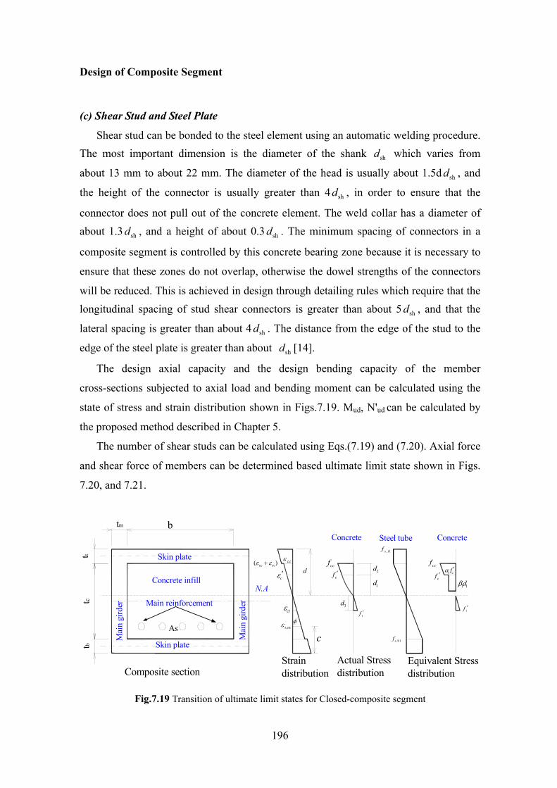
Design of Composite Segment
196
(c) Shear Stud and Steel Plate
Shear stud can be bonded to the steel element using an automatic welding procedure. The most important dimension is the diameter of the shank shd which varies from
about 13 mm to about 22 mm. The diameter of the head is usually about 1.5d shd , and
the height of the connector is usually greater than 4 shd , in order to ensure that the
connector does not pull out of the concrete element. The weld collar has a diameter of about 1.3 shd , and a height of about 0.3 shd . The minimum spacing of connectors in a
composite segment is controlled by this concrete bearing zone because it is necessary to
ensure that these zones do not overlap, otherwise the dowel strengths of the connectors
will be reduced. This is achieved in design through detailing rules which require that the longitudinal spacing of stud shear connectors is greater than about 5 shd , and that the
lateral spacing is greater than about 4 shd . The distance from the edge of the stud to the
edge of the steel plate is greater than about shd [14].
The design axial capacity and the design bending capacity of the member
cross-sections subjected to axial load and bending moment can be calculated using the
state of stress and strain distribution shown in Figs.7.19. Mud, N'ud can be calculated by
the proposed method described in Chapter 5.
The number of shear studs can be calculated using Eqs.(7.19) and (7.20). Axial force
and shear force of members can be determined based ultimate limit state shown in Figs.
7.20, and 7.21.
tttb
tc
tm
,t1sf
,b1sfAs
c
Main reinforcement
s,mε
b
φ
cc st( )ε ε+
Equivalent Stressdistribution
Concrete
Mai
n gi
rder
Mai
n gi
rder 3d
tf ′tf ′
1 cfα ′
1 1dβcf ′
ccf2d
1d
dccf
cf ′
N.A
ctε
ccε
cε ′
Actual Stress distribution
Steel tubeConcrete
Strain distribution
Skin plate
Concrete infill
Skin plate
Composite section
Fig.7.19 Transition of ultimate limit states for Closed-composite segment
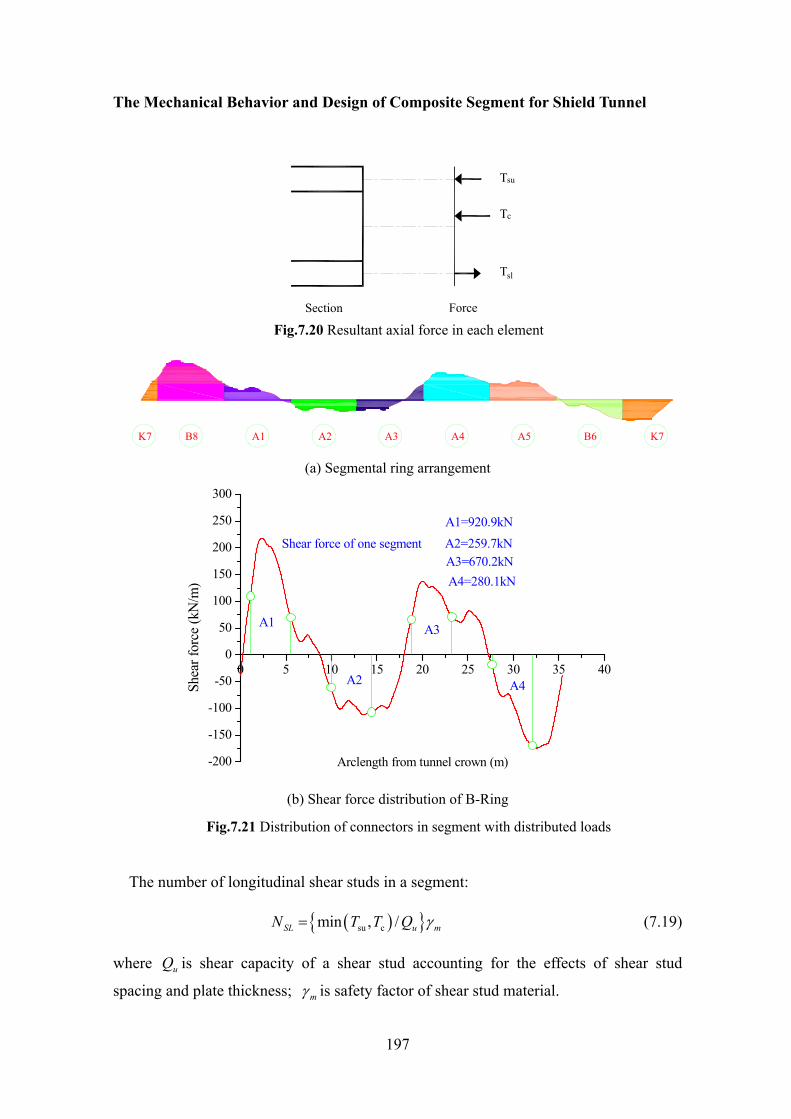
The Mechanical Behavior and Design of Composite Segment for Shield Tunnel
197
Section Force
Tsu
Tc
Tsl
Fig.7.20 Resultant axial force in each element
B8 A1 A2 A3 A4 A5 B6 K7K7
(a) Segmental ring arrangement
0 5 10 15 20 25 30 35 40
-200
-150
-100
-50
0
50
100
150
200
250
300
A4=280.1kNA3=670.2kNA2=259.7kNShear force of one segmentA1=920.9kN
A4
A3
A2
A1
Shea
r for
ce (k
N/m
)
Arclength from tunnel crown (m)
(b) Shear force distribution of B-Ring
Fig.7.21 Distribution of connectors in segment with distributed loads
The number of longitudinal shear studs in a segment:
( ){ }su cmin , /SL u mN T T Q γ= (7.19)
where uQ is shear capacity of a shear stud accounting for the effects of shear stud
spacing and plate thickness; mγ is safety factor of shear stud material.
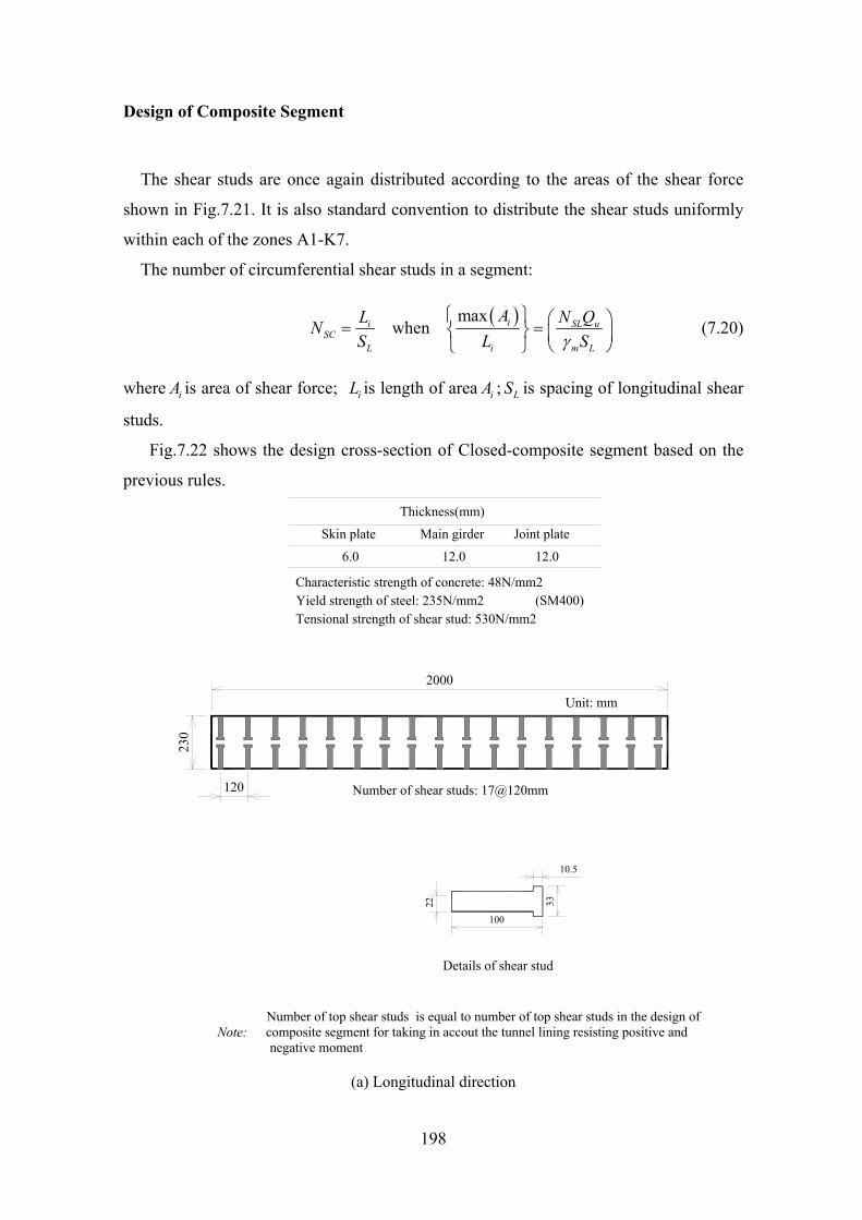
Design of Composite Segment
198
The shear studs are once again distributed according to the areas of the shear force
shown in Fig.7.21. It is also standard convention to distribute the shear studs uniformly
within each of the zones A1-K7.
The number of circumferential shear studs in a segment:
( )maxwhen ii SL u
SCL i m L
AL N QNS L Sγ
⎧ ⎫ ⎛ ⎞= =⎨ ⎬ ⎜ ⎟⎝ ⎠⎩ ⎭
(7.20)
where iA is area of shear force; iL is length of area iA ; LS is spacing of longitudinal shear
studs.
Fig.7.22 shows the design cross-section of Closed-composite segment based on the
previous rules.
230
2000
Unit: mm
Thickness(mm)
Skin plate Main girder Joint plate
6.0 12.0 12.0
Details of shear stud
Characteristic strength of concrete: 48N/mm2Yield strength of steel: 235N/mm2 (SM400)Tensional strength of shear stud: 530N/mm2
10.5
33
100
22
120 Number of shear studs: 17@120mm
Number of top shear studs is equal to number of top shear studs in the design of composite segment for taking in accout the tunnel lining resisting positive and negative moment
Note:
(a) Longitudinal direction
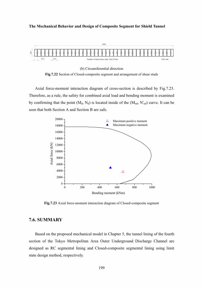
The Mechanical Behavior and Design of Composite Segment for Shield Tunnel
199
230
4550
Unit: mm87.5 Number of lateral shear studs: 36@125mm125
(b) Circumferential direction
Fig.7.22 Section of Closed-composite segment and arrangement of shear studs
Axial force-moment interaction diagram of cross-section is described by Fig.7.23.
Therefore, as a rule, the safety for combined axial load and bending moment is examined
by confirming that the point (Md, Nd) is located inside of the (Mud, N'ud) curve. It can be
seen that both Section A and Section B are safe.
0 200 400 600 800 10000
2000
4000
6000
8000
10000
12000
14000
16000
18000
20000 Maximum positive moment Maximum negative moment
Axi
al fo
rce
(kN
)
Bending moment (kNm) Fig.7.23 Axial force-moment interaction diagram of Closed-composite segment
7.6. SUMMARY
Based on the proposed mechanical model in Chapter 5, the tunnel lining of the fourth
section of the Tokyo Metropolitan Area Outer Underground Discharge Channel are
designed as RC segmental lining and Closed-composite segmental lining using limit
state design method, respectively.
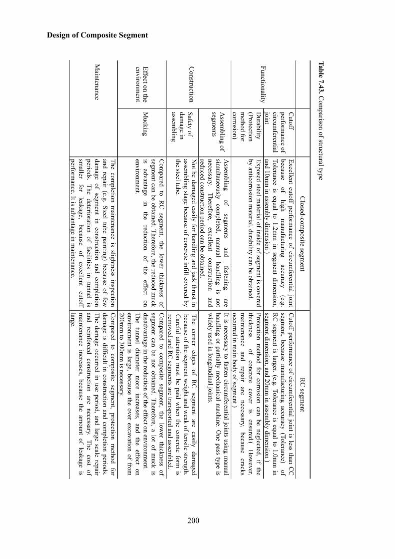
Design of C
omposite Segm
ent
200
Closed-com
posite segment
RC
segment
Cutoff
performance of
circumferential
joint
Excellent cutoff performance of circum
ferential joint because
of high
manufacturing
accuracy (e.g.
Tolerance is equal to 1.2mm
in segment dim
ension, and 10m
m in assem
bly dimension )
Cutoff perform
ance of circumferential joint is less than C
C
segment, because m
anufacturing accuracy (Tolerance) of R
C segm
ent is larger. (e.g. Tolerance is equal to 1.0mm
in segm
ent dimension, and 20m
m in assem
bly dimension )
FunctionalityD
urability (Protection m
ethod for corrosion)
Exposed steel material of inside of segm
ent is covered by anticorrosion m
aterial, durability can be obtained.
Protection method for corrosion can be neglected, if the
thickness
of concrete
cover is
ensured.( H
owever,
maintenance
and repair
are necessary,
because cracks
occurred in main body of segm
ent )
Assem
bling of segm
ents
Assem
bling of
segments
and fastening
are sim
ultaneously com
pleted, m
anual handling
is not
necessary. Therefore,
excellent construction
and reduced construction period can be obtained.
It is necessary to fasten circumferential joints using m
anual handling or partially m
echanical machine. O
ne pass type is w
idely used in longitudinal joints.
Construction
Safety of dam
age in assem
bling
Not be dam
aged easily for handling and jack thrust in assem
bling stage because of concrete infill covered by the steel tube.
The corner edges of RC
segment are easily dam
aged because of the segm
ent weight and w
eak of tensile strength. C
areful attention must be paid w
hen the concrete form is
removed and R
C segm
ents are transported and assembled.
Effect on the environm
ent M
ucking
Com
pared to RC
segment, the low
er thickness of segm
ent can be obtained. Therefore, the reduced muck
is advantage
in the
reduction of
the effect
on environm
ent.
Com
pared to composite segm
ent, the lower thickness of
segment can be not obtained. Therefore, a lot of m
uck is disadvantage in the reduction of the effect on environm
ent. The tunnel diam
eter more increases, and the effect on
environment is large, because the over excavation of from
200m
m to 300m
m is necessary.
Maintenance
The completion m
aintenance is slightness inspection and repair (e.g. Steel tube painting) because of few
dam
age of segment in construction and com
pletion periods. The deterioration of facilities in tunnel is sm
aller for
leakage, because
of excellent
cutoff perform
ance. It is advantage in maintenance.
Com
pared to composite segm
ent, protection method for
damage is difficult in construction and com
pletion periods. The dam
age occurred in use period, and large scale repair and
reinforced construction
are necessary.
The cost
of m
aintenance increases, because the amount of leakage is
large.
Table 7.43. Com
parison of structural type
200
Design of Composite Segment
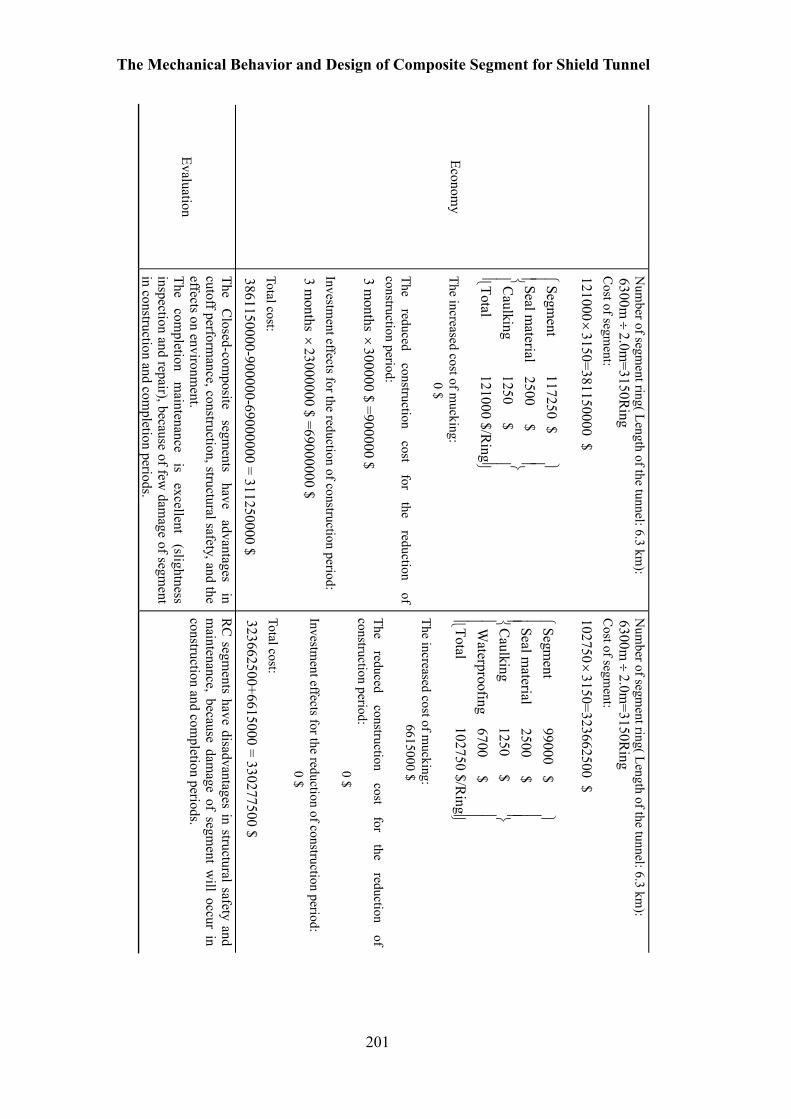
The M
echanical Behavior and D
esign of Com
posite Segment for Shield Tunnel
201
Economy
Num
ber of segment ring( Length of the tunnel: 6.3 km
): 6300m
2.0m=3150R
ing÷
C
ost of segment:
1210003150=381150000 $
×
Segment
117250 $ Seal m
aterial2500 $
Caulking
1250 $Total
121000 $/Ring
⎧⎫
⎪⎪
⎪⎪
⎨⎬
⎪⎪
⎪⎪
⎩⎭
The increased cost of mucking:
0 $ The
reduced construction
cost for
the reduction
of construction period: 3 m
onths 300000 $ =900000 $
×
Investment effects for the reduction of construction period:
3 months
23000000 $ =69000000 $×
Total cost: 3861150000-900000-69000000 = 311250000 $
Num
ber of segment ring( Length of the tunnel: 6.3 km
): 6300m
2.0m=3150R
ing÷
C
ost of segment:
1027503150=323662500 $
×
Segment
99000 $Seal m
aterial2500 $
Caulking
1250 $W
aterproofing6700 $
Total102750 $/R
ing
⎧⎫
⎪⎪
⎪⎪
⎪⎪
⎨⎬
⎪⎪
⎪⎪
⎪⎪
⎩⎭
The increased cost of mucking:
6615000 $ The
reduced construction
cost for
the reduction
of construction period: 0 $ Investm
ent effects for the reduction of construction period: 0 $
Total cost: 323662500+6615000 = 330277500 $
Evaluation
The C
losed-composite
segments
have advantages
in cutoff perform
ance, construction, structural safety, and the effects on environm
ent. The
completion
maintenance
is excellent
(slightness inspection and repair), because of few
damage of segm
ent in construction and com
pletion periods.
RC
segments have disadvantages in structural safety and
maintenance, because dam
age of segment w
ill occur in construction and com
pletion periods.
The Mechanical Behavior and Design of Composite Segment for Shield Tunnel
201
Design of Composite Segment
202
Comparisons have been made between the cross-section of RC segment and the
cross-section of Closed-composite segment shown in Table 7.43. The reduction of
segment thickness is obtained using Closed-composite segment and this indicates that
Closed-composite segment is suitable for decreasing muck, construction period and the
outside diameter of the shield machine. In general, the costs of construction, risk, and
maintenance will be decreased
7.7. REFERENCES
1) International tunnelling association, 2000. Guidelines for the design of shield tunnel
lining. Tunnelling and Underground Space Technology, Vol. 15, No. 3, pp. 303-331.
2) Japanese Society of Civil Engineers (JSCE), 2007. Standard specifications for
tunneling-2006, Shield tunnels.
3) Japanese Society of Civil Engineers (JSCE), 1994. Standard specifications for design
segment (in Japanese).
4) Terzaghi, K., 1946. Rock Defects and Load on Tunnel Supports. In: Proctor, R.V.,
White, T.C. (Eds.), Introduction to Rock Tunnelling with Steel Support. Commercial
Shearing and Stamping Co., Youngstava, OH, USA.
5) Railway Technical Research Institute (RTRI), 1997. Design Standard for Railway
Structures (Shield-Driven Tunnel), Maruzen, pp. 47-61. (In Japanese)
6) Murakami, Koizumi, et al, 1978. Study on rational design method of the
circumferential joint of a segment. Waseda Univ. report, No.82. (In Japanese)
7) Koizumi, 1979. Study on segment design. Ph.D. thesis, Waseda Univ., Tokyo. (In
Japanese)
8) Koizumi, Murakami, Nishino,1988. Study on the analytical model for shield tunnel in
longitudinal direction. Journal of JSCE, No.394, 1-10. (In Japanese)
9) Kimura, Koizumi, 1999. A design method of shield tunnel lining taking in account of
the interaction between the lining and the ground. Journal of JSCE, No.624, 123-134.
(In Japanese)
10) Japanese Society of Civil Engineers (JSCE), 2003. Standard specifications for
concrete structures-2002, Structural performance verification.

The Mechanical Behavior and Design of Composite Segment for Shield Tunnel
203
11) Masami, Shirato, et al.2003. Development of new composite segment and
application to the tunneling project. Journal of JSCE, No.728, 157-174.(In Japanese)
12) Galambos TV, 1998. Guide to stability design criteria for metal structures.5th ed.
New York: Wiley.
13) Montoya, E.,2003. Behavior and analysis of confined concrete. Ph.D. thesis, Univ. of
Toronto, Toronto.
14) Deric J Oehlers, Mark A Bradford, 1995. Composite steel and concrete structural
members. UK: Pergamon, Elsevier Science.

The Mechanical Behavior and Design of Composite Segment for Shield Tunnel
205
Chapter 8. Conclusions
The mechanical behavior of composite segment with different composited designs is
investigated in this paper. The local buckling, slip and effective strength formulas are
incorporated into the nonlinear analysis procedures to account for local buckling and slip
effects on the strength and ductility performance of composite segments under combined
loads. From the results described in previous chapters, several conclusions may be
summarized as follows.
(a) The accuracy of proposed FEM models
A comparison between the analyzed and experimental results indicates that the
proposed finite element model using MSC.Marc can simulate the mechanical behavior
of composite segments (including Closed-composite segment, SSPC segment, and DRC
segment).
Contact analysis was found to be able to simulate the slip at the interface between
steel tube and concrete infill. For the composite segments with no axial load, frictionless
condition could simulate the load-deflection curves from the experimental results. For
axially loaded the composite segments, a friction coefficient of 0.1 produced convincing
results.
Discrete shear studs modeled using 3D beam elements is able to simulate the
mechanical behavior of shear connectors.
The effective width of the skin plate in compression should be adopted in analysis
and design of composite segment, according to different degree of shear connection. The
skin plate in tension can be assumed as the member of full effective cross-section.
(b) The accuracy of proposed mechanical model
A nonlinear fiber element analysis method is proposed for the inelastic analysis and
design of concrete infill steel tubular composite segments with local buckling and slips.
Sectional geometry, residual stresses and strain hardening of steel tubes and confined
concrete models were considered in the proposed mechanical model. The local buckling,
slip and effective strength formulas were incorporated into the nonlinear analysis

Conclusion
206
procedures to account for local buckling and slip effects on the strength and ductility
performance of composite segments under combined loads.
The formulation of differential equations is suitable for the solution of partially
interactive steel tube composite segment elements. Closed form solutions for single,
double and uniform load arrangements on simple span segments have been presented. A
step-wise linearization method has been described which allows the non-linear affects of
concrete cracking and shear stud stiffness to be incorporated.
The analysis involves non-dimensional constants which affect the steel plate
interaction. The effects are either direct when the constant relates to the plate for which
it is formulated or crossed when it affects the opposite plate for which it is formulated.
More attention should be paid on the shear capacity of shear studs in composite
segments. In current codes, only some coefficients are suggested for considering the
influences of the concrete strength, steel strength, and shear stud dimension. It was
found that the shear stud spacing and the thickness of the welded steel plate also have the effects on the shear capacity, so the coefficients η and Vβ are recommended.
Comparisons are made between experimental results and the mechanical predictions
of behavior using the proposed method. Good agreement is found and this indicates that
the proposed method is suitable for general analysis of tunnel lining of composite
segment.
(c) Design tunnel lining of composite segment
A comparison is made between the cross-section of RC segment and the cross-section
of Closed-composite segment. The reduction of segment thickness is obtained using
Closed-composite segment and this indicates that Closed-composite segment is suitable
for decreasing muck, construction period and the outside diameter of the shield machine.
In general, the costs of construction, risk, and maintenance will be decreased
The Mechanical Behavior and Design of Composite
Segment for Shield Tunnel
Abstract in Japanese

合成セグメントの力学的挙動および設計法
に関する研究
(概要) 張 穏軍
大都市部の地下には,地下鉄をはじめとして,上下水道,電気用とう道,通信用とう
道,ガス管路などのインフラ構造物が数多く構築されている.これらの施設は主な公共
用地である道路下に構築されることが多い.東京都内の国道下だけに限っても,道路1km
あたり約33kmの管路が埋設されている.このほかに都道や区道の下にもトンネルや管路
類が輻輳し,現在では都市部の地下は非常に混雑した状態となっている.
これまでの都市部の地下は,建設が容易な浅いところから順に利用されてきており,
新たに建設される施設は既存の施設より深い道路下に設置せざるを得ないため,その構
築深度は年々深くなりつつある.また,最近では,深い地下を利用した地下河川や地下
貯留管などの整備も数多く行われ,さらにこれに加えて,道路用の大断面のトンネルも
造られるようになってきている.
地下利用においては,大深度化だけではなく,トンネルの大断面化,従来の円形断面
に代わって矩形断面や楕円形断面,多心円形断面などの異形断面化が進んできている.
このため,トンネルには大きな土水圧が作用したり,大きな断面力が発生するなど,シ
ールドトンネルの覆工に用いられるセグメントに付与すべき性能も多様化してきてい
る.
円形断面をもつ大断面のトンネルでは,掘削土量は掘削外径の二乗に比例して増える
ことから,建設発生土の処理コストが増加する.また,シールド機の仮組立て,分割,
運搬,現場での再組立てなどのシールド機の製作コストも増加する.一方で,地下河川
や地下貯留管などを除けば,一般にトンネル断面の中央部のみを有効に利用することが
多く,その上部と下部は余剰な断面となることが多い.トンネルが大断面化するほどこ
れらの影響が顕著になってくる.このため,円形以外の断面を採用して,掘削土量を減
少させる一方で,断面を有効に使用しようとするケースも増えてきている.円形以外の
断面のトンネルを構築する場合には,覆工に発生する断面力や変形が大きくなることが
多く,鉄筋コンクリート製のセグメント(以下,RC セグメントと呼ぶ)を採用した場
合にはセグメントの厚さが厚くならざるを得ない.セグメントが厚くなると,その分重
量が重くなり,セグメント工場における製作性やハンドリング,工場から現場までの運
搬,工事ヤードから坑内への搬入,切羽での組立てなどに大きな労力と神経を使うこと
になり,また,セグメントの損傷なども起きやすくなる.
一方,一次覆工に鋼製セグメントを採用した場合には,トンネルの掘削深度が大きく
なれば大きな土水圧やジャッキ推力,裏込め注入圧などの荷重が作用することになる.
これに必要な耐荷力や剛性を確保するためには相当に厚い鋼板を使わざるをえず,溶接
などの製作上の問題を含めて経済性に疑問が生じる.ダクタイルセグメントを採用した
場合には溶接の問題はないが,鋼製セグメントと同様に製作コストに問題が生じる.こ
れらのことから,鋼のもつ力学的な優位性やコンクリートのもつ経済性に加えて,鋼殻
によるコンクリートの変形拘束効果を期待した合成セグメントが開発されている.合成
セグメントには,RC セグメントの鉄筋を鋼板やラチスガーダー,形鋼などに置き換え
てその外側をコンクリートで覆うもの,鋼製セグメントの内径側に鉄筋を配置してその
内部にコンクリートを中詰めしたもの,4 面または 6 面を鋼殻の内部にコンクリートを
中詰めしたものなど,いくつかのタイプがある.最近では鋼製セグメントや鋼殻の内部
にコンクリートを中詰めしたものが多く使われている.しかし,これらの合成セグメン
トの現行の設計では,主げたを無視して外側および内側のスキンプレートを鉄筋として
評価したり,主げたは考慮してもスキンプレートには有効幅を考えたりすることが多い.
また,その内部に打設されたコンクリートは考慮されずに,二次覆工の代わり程度の役
割として扱われる場合がほとんどである.すなわち,設計上の取り扱いは合成セグメン
トごとに異なるのが実状である.これらの合成セグメントのうちで,スタッドを溶植し
たスキンプレート,主げたプレート,継手プレートからなる六面体の鋼殻の内部に高流
動性のコンクリートを中詰めした合成セグメント(以下,密閉式合成セグメントと呼ぶ)
は,その外側の 6 面が鋼板で囲われているため,内部のコンクリートの挙動が直接観測
できないこと,内部のコンクリートは鋼板やその内側に溶植されたスタッドジベルによ
る変形の拘束効果を受けると想像されることなどから,その耐荷機構は力学的にもっと
も複雑なものであると考えられる.
本研究は,密閉式合成セグメントの耐荷機構を明らかにして,その合理的な設計手法
を提案するとともに,それが類似の合成セグメントにも適用できることを示したもので
ある.
本研究では,まず,密閉式合成セグメントの模型供試体を作製して載荷試験を行い,
その結果に考察を加え,有限要素法による非線形解析や鉄筋コンクリート理論(以下,
RC 理論と略称する)に準拠した解析を行った.それらの結果から,密閉式合成セグメ
ントの耐荷機構を明らかにし,その降伏曲げ耐力,終局耐力,変形の具体的な算定手法
を提案した.つぎに,鋼製セグメントにコンクリートを中詰めしただけのセグメントと
ダクタイルセグメントの内径側に鉄筋を配置してコンクリートを中詰めしたセグメン
トの実験結果を用いて,提案した算定手法がそのほかの類似の合成セグメントにも適用
可能かどうかを検証した.最後に,密閉式合成セグメントの優位性を検討する目的で,
提案した算定手法により,首都圏外郭放水路第4工区のセグメントを対象として,限界
状態設計法にもとづいた試設計を行った.結果として,密閉式合成セグメントは,RC
セグメントと比べて,セグメントの薄肉化が可能であり,総合的な工費を縮減できるこ
とがわかった.
本論文は 8 章より構成されおり,その概要は以下のとおりである.
第 1 章は,研究の背景,目的および論文の構成について記述した章である.
第 2 章では,合成セグメントに用いられる材料の材料特性に関する既往の研究をレビ
ューし,精度が高い材料モデルを検討している.
第 3 章は,密閉式合成セグメント模型の載荷試験にもとづいて,その挙動を評価した
章である.ここでは,まず,模型供試体の寸法,使用した材料,ずれ止めの配置,測定
項目および載荷方法などについて詳述した.つぎに,密閉式合成セグメント模型の載荷
試験を行い,その結果から,耐荷性能を損なう要因として,鋼とコンクリートとの境界

面に生じるずれ,スキンプレートの局部座屈,ずれ止め位置におけるコンクリートの局
所破壊などが考えられ,これらが密閉式合成セグメント模型の曲げ耐力に大きな影響を
与えることが明らかになった.すなわち,密閉式合成セグメント模型は,隣接する 2 本
のスタッドジベル間の圧縮側スキンプレートに局部座屈が生じた後も圧縮側スキンプ
レートは圧縮耐力を保持し,圧縮ひずみが終局ひずみに達したときに,中詰めコンクリ
ートが圧壊することにより破壊に至る.
第 4 章は 3 次元材料非線形 FEM を用いて,密閉式合成セグメント模型の耐荷機構を
検討した章である.3 次元材料非線形 FEM による解析結果は,載荷試験におけるスタッ
ドジベルの効果をよく表現できた.また,曲げ耐力および破壊モードの解析結果は実験
結果のそれらと一致し,両者の変形挙動もほぼ表現できた.
第 5 章は,載荷試験結果と FEM による解析結果をもとに,曲げと軸力との組合せ荷
重を受ける密閉式合成セグメント模型の降伏曲げ耐力,終局曲げ耐力および変形の算定
手法を提案した章である.この章では,密閉式合成セグメント既往の実験結果を用いて,
提案した算定手法の妥当性も検証した.結果として,提案した算定手法は密閉式合成セ
グメントの降伏曲げ耐力,終局曲げ耐力および変形を精度よく算定できることを示した.
第 6 章は,その他の合成セグメントへの適用性を検討したものである.この章では,
コンクリート中詰め鋼製セグメントおよびコンクリート中詰めダクタイルセグメント
についての FEM 解析を行い,その結果とそれらの既往の実験結果とを比較検討すると
ともに,提案した算定手法および FEM モデルの適用性も検証した.
第 7 章は提案した算定手法を用いて合成セグメントを試設計したものである.
試設計の対象は首都圏外郭放水路第4工区であり,密閉式合成セグメントを限界状態
設計法にもとづいて設計した.試設計の結果をみると,密閉式合成セグメントは,RC
セグメントと比べて,セグメントの薄肉化が図れ,セグメントの組立時間の短縮などを
総合的に考えると,工費の縮減が期待できることがわかった.
第 8 章は結論を述べた章であり,第 2 章から第 7 章で得られた主要な研究成果を要約
して述べている.

List of Papers


早稲田大学 博士(工学) 学位申請 研究業績書
氏 名 張 穏軍 印
(2009 年 10 月 現在)
種 類 別 題名、 発表・発行掲載誌名、 発表・発行年月、 連名者
(申請者含む)
1. 論文
論文
○ 論文
○ 論文
○ 論文
○ 論文
○ 論文
A study of the localized bearing capacity of reinforced concrete K-segment,Tunnelling and Underground Space Technology, ITA, Vol.22,No.4, pp.467-473, 2007,7. Wenjun Zhang, Atsushi Koizumi.
密閉式合成セグメントの鋼コンクリート界面の相対ずれに関する研究,
現代トンネル技術, 第4回日中シールド技術交流会,広州,中国,pp.40-45, 2007,9.張 穏軍,小泉 淳.
Flexural rigidity of closed composite segment, Proceedings of the International Symposium on Tunnelling for Urban Development, ITA, Pattaya, Thailand, pp.205-212, 2007,12. Wenjun Zhang, Atsushi Koizumi.
Stiffness and Deflection of Composite Segment for Shield Tunnel, Tunnelling Technology & The Environment, TAC, Canada, pp.95-105, 2008,10. Wenjun Zhang, Atsushi Koizumi.
合成セグメントの曲げ挙動に関する研究,土木学会論文集 F, Vol.65,No2, pp.246-263, 2009.張 穏軍,小泉 淳.
Design of composite segment for underground discharge channel, Proceedings of the fifth China-Japan conference on shield tunnelling, Chengdu, China, pp.10-19, 2009,9. Wenjun Zhang, Atsushi Koizumi.
2. 報告
報告
ジャッキ推力による鋼製セグメントの座屈挙動に関する研究,土木学会
トンネル工学研究発表会論文報告集,第 16 巻,pp.319~324,2006,鈴木哲
太郎,張 穏軍,小泉 淳.

3. 著書
訳書
訳書
シールド工法の調査・設計から施工まで(中国語版),中国建築工業出版
社,2008,ISBN 978-7-112-09246-8, 監訳:張 穏軍.
シールドトンネルの耐震検討(中国語版),中国建築工業出版社,2009,
ISBN 978-7-112-10949-4, 監訳:張 穏軍.
4. 講演
○ 講演 講演 講演 講演
○ 講演
合成セグメントの設計,JR 東日本発表会,2007 年 3 月,張 穏軍.
覆工版の設計,北京交通大学,2006 年 7 月,小泉 淳, 張 穏軍.
シールド工法,瀋陽地下鉄会社,2006 年 7 月,小泉 淳, 張 穏軍.
シールド工法とセグメントの設計,大連理工大学,2006 年 7 月,小泉 淳,
張 穏軍.
合成セグメントの力学的挙動および設計法に関する研究,みずほ情報総
研株式会社,2009 年 9 月,張 穏軍.
5.その他
鋼構造研
究助成費
合成セグメントの力学的なメカニズムに関する研究,社団法人日本鉄鋼
連盟(JISF),2008, 300 万円,張 穏軍.