single sourse shortest paths: formulation - gabriel...

Single sourse shortest paths: formulation

GIVEN: weighted, directed graph G = (V, E), weight function w : E → R.

Weight of path p = (v0, v1, . . . , vk):

w(p) =

kX

i=1

w(vi−1, vi).

Shortest path weight from u to v:

δ(u, v) =

8

<

:

min{w(p)} if u v,

∞ otherwise.

Shortest path from u to v: every path p with w(p) = δ(u, v).

Single source shortest path: Given a graph G = (V, E) find a shortest path from anode u to each vertex v ∈ V .

BFS: shortest path in unweighted graphs.

Data Structures – p.1/32

Formulation (II)

Same algorithms can solve many variants:

Single destination shortest path. Find shortest paths from all nodes to a given node.

Single pair shortest path. No algorithm known that is asymptotically faster for thisproblem.

All-pairs shortest paths: we’ll study this problem on its own.


Optimal substructure property

Informally: A shortest path contain other shortest paths within it.

Hallmark of both dynamic programming and greedy.

Dijkstra: greedy, Floyd-Warshall dynamic programming.

Each task could be specified in terms of input and output.

Lemma 1 Given weighted, directed graph G = (V, E) with weight function w, letp = (v1, . . . vk) be a shortest path from v1 to vk and, for any 1 ≤ i < j ≤ k let pi,j thesubpath of p from vi to vj . Then pi,j is a shortest path.


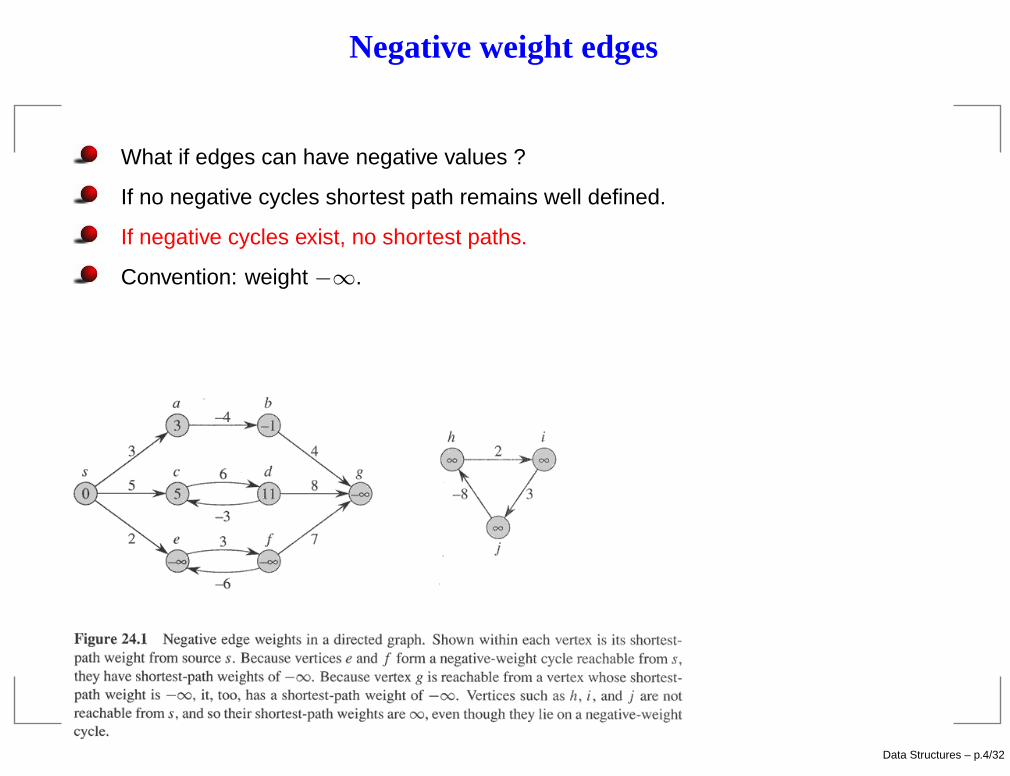
Negative weight edges

What if edges can have negative values ?

If no negative cycles shortest path remains well defined.

If negative cycles exist, no shortest paths.

Convention: weight −∞.


Positive weight cycles

No shortest path can contain any positive weight cycles.

0-weight cycles: can be eliminated from shortest path to produce another shortestpath with fewer edges.

Without loss of generality: acyclic shortest paths. At most |V | − 1 edges.

Representing shortest paths: like BFS trees. π[v] predecessor of v. Either anothervertex or NIL.

Can "go backwards" on π to print shortest paths.

During the execution of algorithm π does not indicate shortest paths.

Predecessor subgraph: Gπ = (Vπ , Eπ).

Vπ = {v ∈ V : π[v] 6= NIL} ∪ {s}.

Eπ = {(π[v], v) ∈ E : v ∈ Vπ \ {s}}.

At termination Gπ is a shortest path tree.


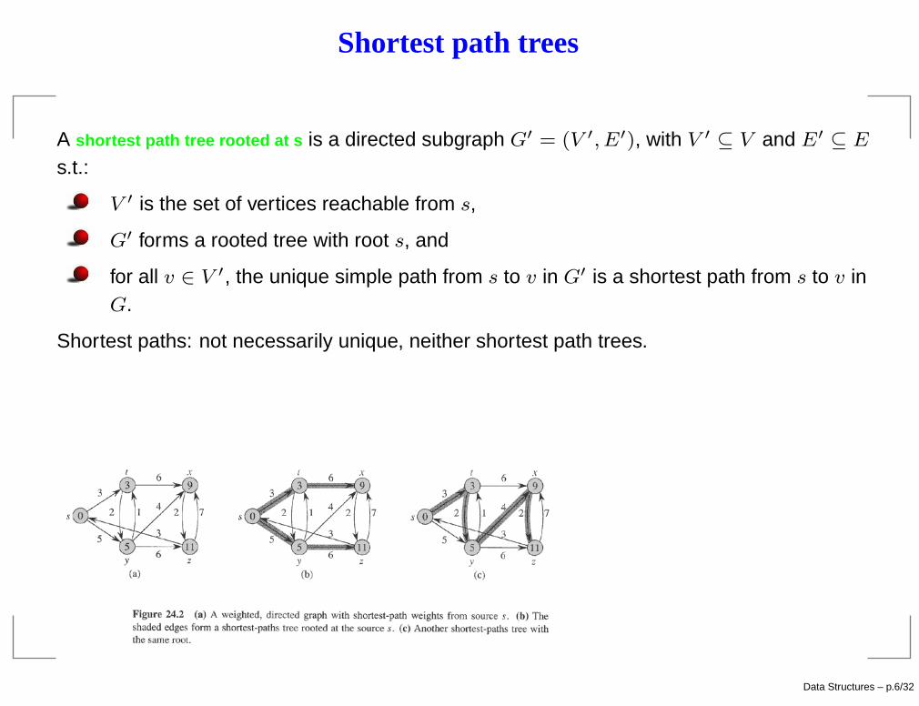
Shortest path trees

A shortest path tree rooted at s is a directed subgraph G′ = (V ′, E′), with V ′ ⊆ V and E′ ⊆ E

s.t.:

V ′ is the set of vertices reachable from s,

G′ forms a rooted tree with root s, and

for all v ∈ V ′, the unique simple path from s to v in G′ is a shortest path from s to v inG.

Shortest paths: not necessarily unique, neither shortest path trees.


Relaxation

Common technique for algorithms in this section.

We maintain an attribute d[v], upper bound on distance from s to v. shortest pathestimate.

Initialization: θ(|V |).

INITIALIZE-SINGLE-SOURCE(G,s){

for each v ∈ V [G]

{

d[v] = ∞;

π[v] = NIL;

}

d[s]=0;

}


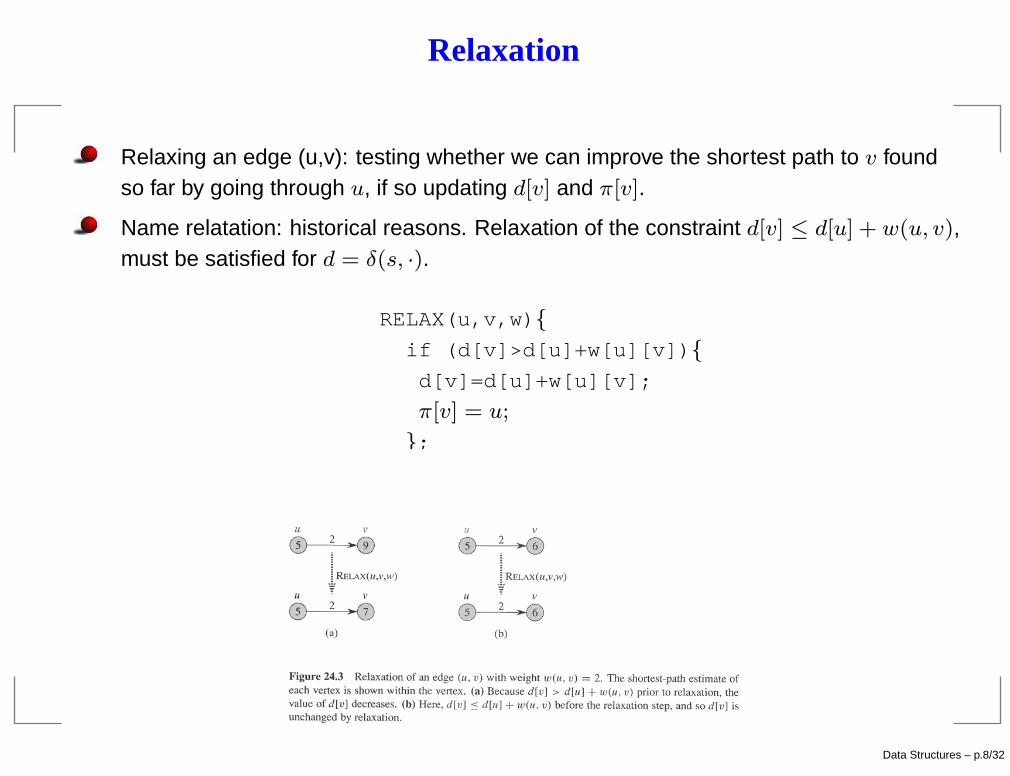
Relaxation

Relaxing an edge (u,v): testing whether we can improve the shortest path to v foundso far by going through u, if so updating d[v] and π[v].

Name relatation: historical reasons. Relaxation of the constraint d[v] ≤ d[u] + w(u, v),must be satisfied for d = δ(s, ·).

RELAX(u,v,w){

if (d[v]>d[u]+w[u][v]){

d[v]=d[u]+w[u][v];

π[v] = u;

};

}


Properties of shortest paths and relaxation

For correctness purposes following lemmas, proofs omitted.

Triangle inequality: for any edge (u, v) ∈ E, δ(s, v) ≤ δ(s, u) + w(u, v).

Upper bound property: Always d[v] ≥ δ(s, v). Once d[v] becomes equal to δ(s, v) itnever changes.

No path property: If there is no path from s to v then always d[v] = δ(s, v) = ∞.

Path-relaxation property: If p = (v0, . . . , vk) is a shortest path from s = v0 to vk andthe edges of p are relaxed in the order (v0, v1, (v1, v2), . . . , (vk−1, vk) thend[vk] = δ(s, vk). This holds irrespective of other relaxations.

Predecessor-subgraph property: Once d[v] = δ(s, v) for all v ∈ V , the predecessorsubgraph is a shortest-path tree rooted at s.


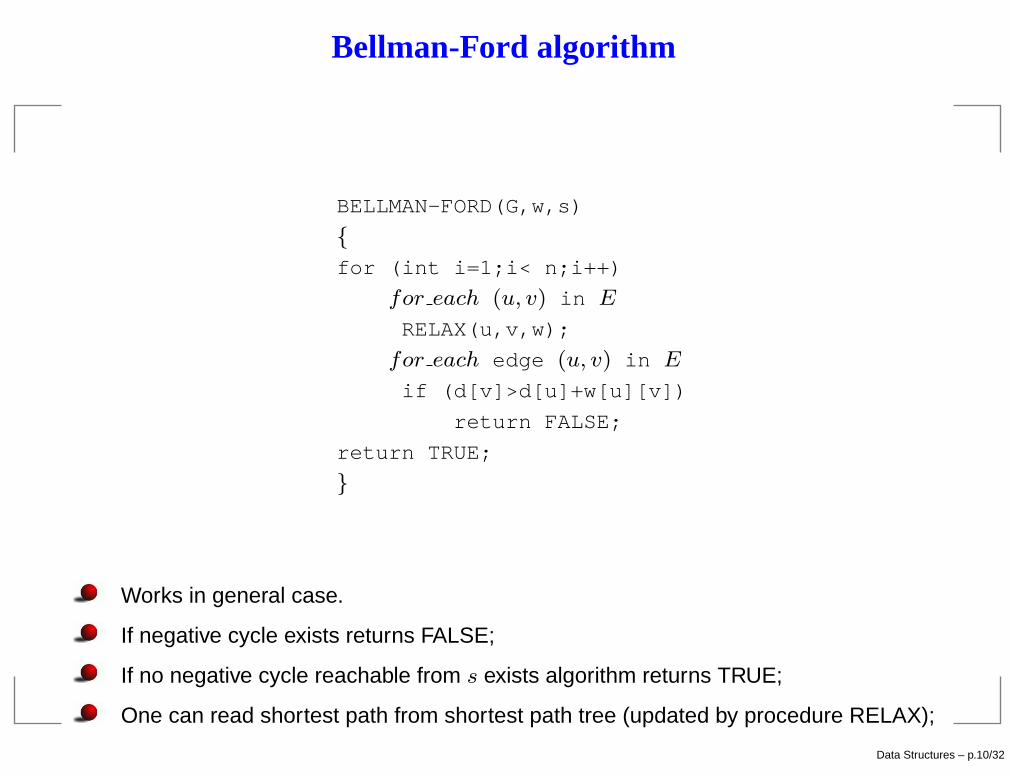
Bellman-Ford algorithm

BELLMAN-FORD(G,w,s)

{

for (int i=1;i< n;i++)

for each (u, v) in E

RELAX(u,v,w);

for each edge (u, v) in E

if (d[v]>d[u]+w[u][v])

return FALSE;

return TRUE;

}

Works in general case.

If negative cycle exists returns FALSE;

If no negative cycle reachable from s exists algorithm returns TRUE;

One can read shortest path from shortest path tree (updated by procedure RELAX);


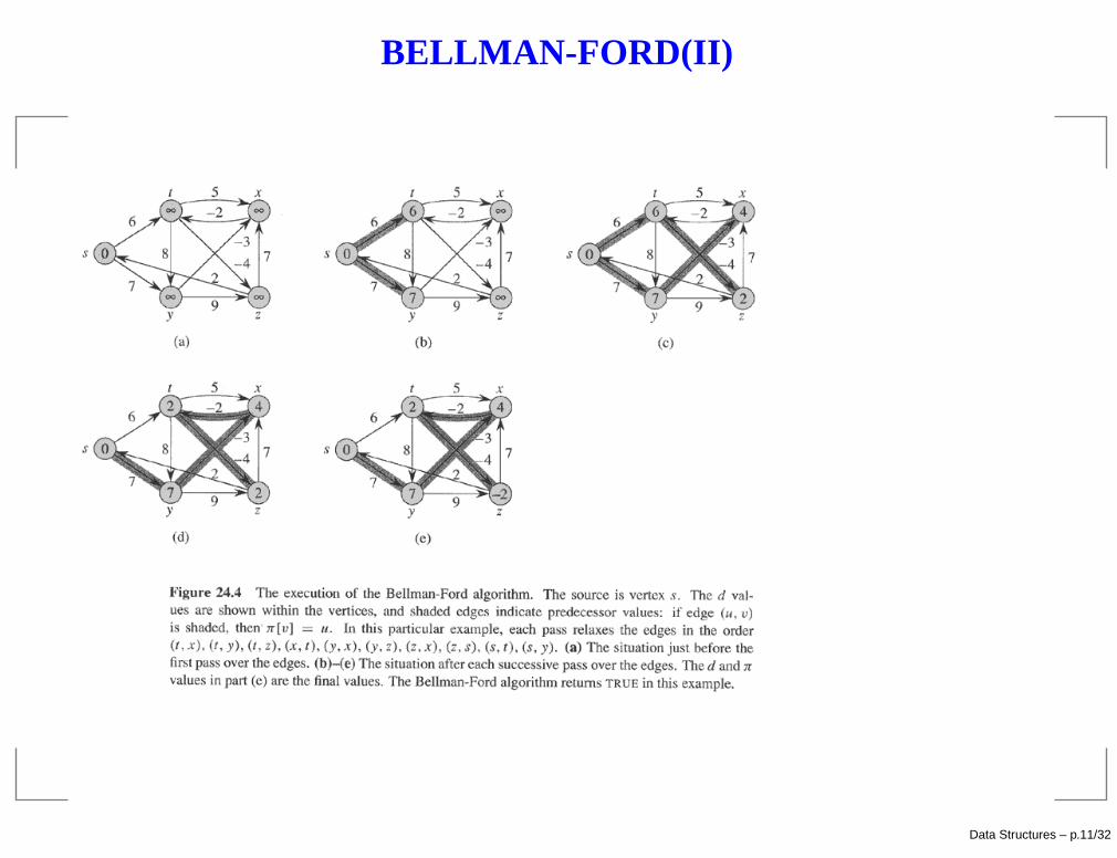
BELLMAN-FORD(II)


Bellman-Ford: Analysis and Implementation

Running time: θ(|V | · |E|). Main loop |V | times, each of them complexity θ(|E|).

Correctness: path-relaxation property.

Member data to the SP class: d, π, w a list of vertices, a list of edges. Memberfunction RELAX.


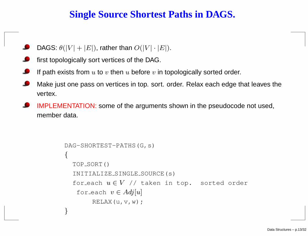
Single Source Shortest Paths in DAGS.

DAGS: θ(|V | + |E|), rather than O(|V | · |E|).

first topologically sort vertices of the DAG.

If path exists from u to v then u before v in topologically sorted order.

Make just one pass on vertices in top. sort. order. Relax each edge that leaves thevertex.

IMPLEMENTATION: some of the arguments shown in the pseudocode not used,member data.

DAG-SHORTEST-PATHS(G,s)

{

TOP SORT()

INITIALIZE SINGLE SOURCE(s)

for each u ∈ V // taken in top. sorted order

for each v ∈ Adj[u]

RELAX(u,v,w);

}


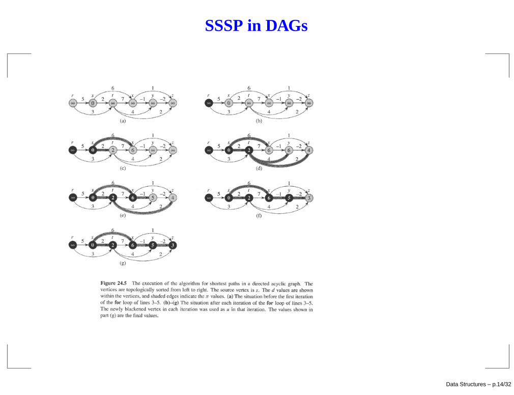
SSSP in DAGs


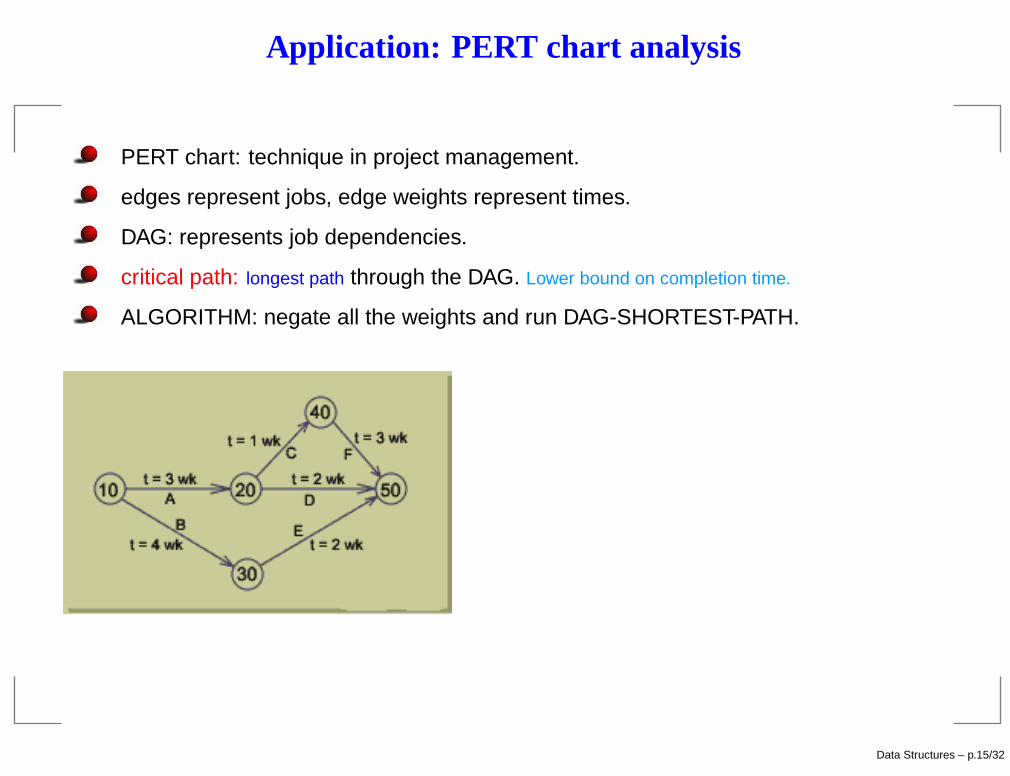
Application: PERT chart analysis

PERT chart: technique in project management.

edges represent jobs, edge weights represent times.

DAG: represents job dependencies.

critical path: longest path through the DAG. Lower bound on completion time.

ALGORITHM: negate all the weights and run DAG-SHORTEST-PATH.


Application: Difference constraints and shortest paths

Linear programming: m × n matrix A, m-vector B, n-vector C.

Want to find: vector x of n elements that maximizes the objective functionPn

i=1 cixi subjectto the m constraints Ax.

Simplex algorithm: randomized version runs in polynomial time (research result 2006)

More complicated method (ellipsoid method): polynomial time (worst case)

Feasibility problem: find feasible solution for Ax ≤ b or determine that none exists.

For vectors: x ≤ y if xi ≤ yi (componentwise inequalities).


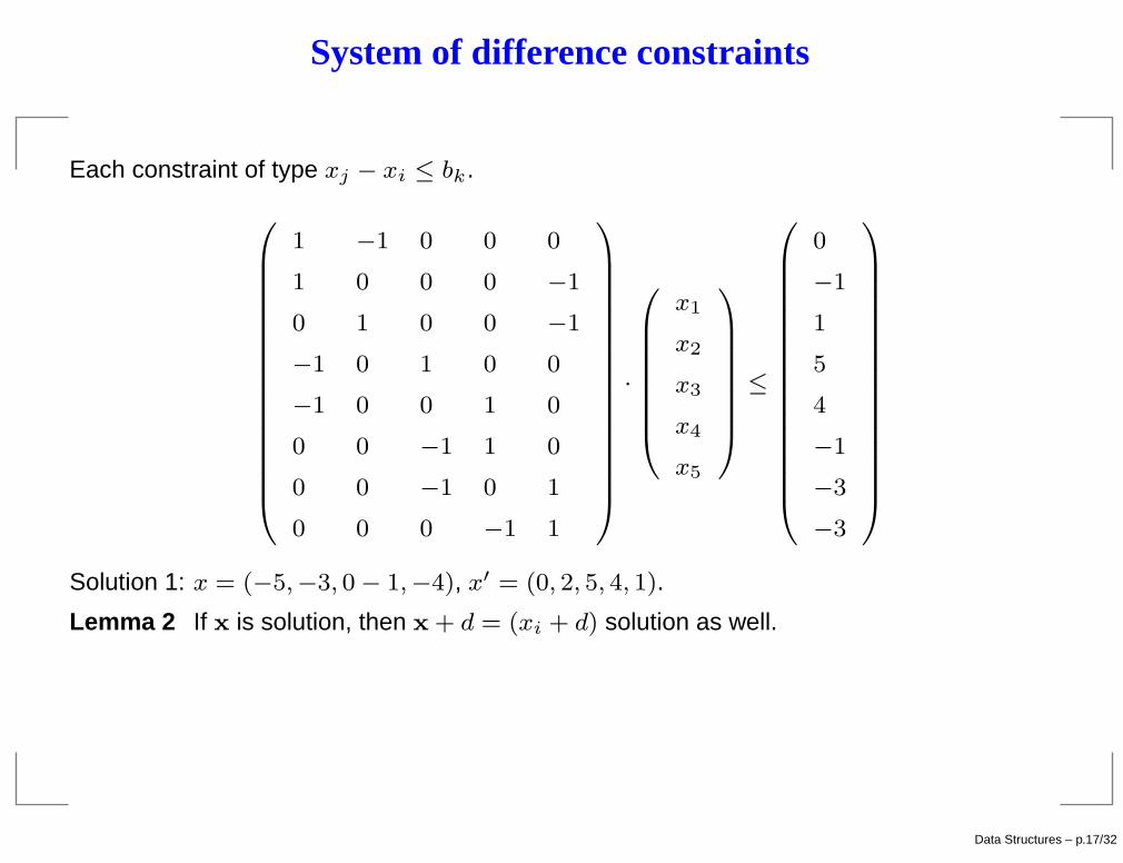
System of difference constraints

Each constraint of type xj − xi ≤ bk.

0

B

B

B

B

B

B

B

B

B

B

B

B

B

B

B

B

@

1 −1 0 0 0

1 0 0 0 −1

0 1 0 0 −1

−1 0 1 0 0

−1 0 0 1 0

0 0 −1 1 0

0 0 −1 0 1

0 0 0 −1 1

1

C

C

C

C

C

C

C

C

C

C

C

C

C

C

C

C

A

·

0

B

B

B

B

B

B

B

@

x1

x2

x3

x4

x5

1

C

C

C

C

C

C

C

A

≤

0

B

B

B

B

B

B

B

B

B

B

B

B

B

B

B

B

@

0

−1

1

5

4

−1

−3

−3

1

C

C

C

C

C

C

C

C

C

C

C

C

C

C

C

C

A

Solution 1: x = (−5,−3, 0 − 1,−4), x′ = (0, 2, 5, 4, 1).

Lemma 2 If x is solution, then x + d = (xi + d) solution as well.


Constraint graphs

Each node corresponds to a variable.

Each directed edge corresponds to an inequality.

V = {v0, v1, . . . , vn}.

E = {(vi, vj) : xi − xj ≤ bk} ∪ {(v0, v1), (v0, v2), . . . , (v0, vn)}.

edge (vi, vj): edge weight bk.

weights: 0 for edges from v0.


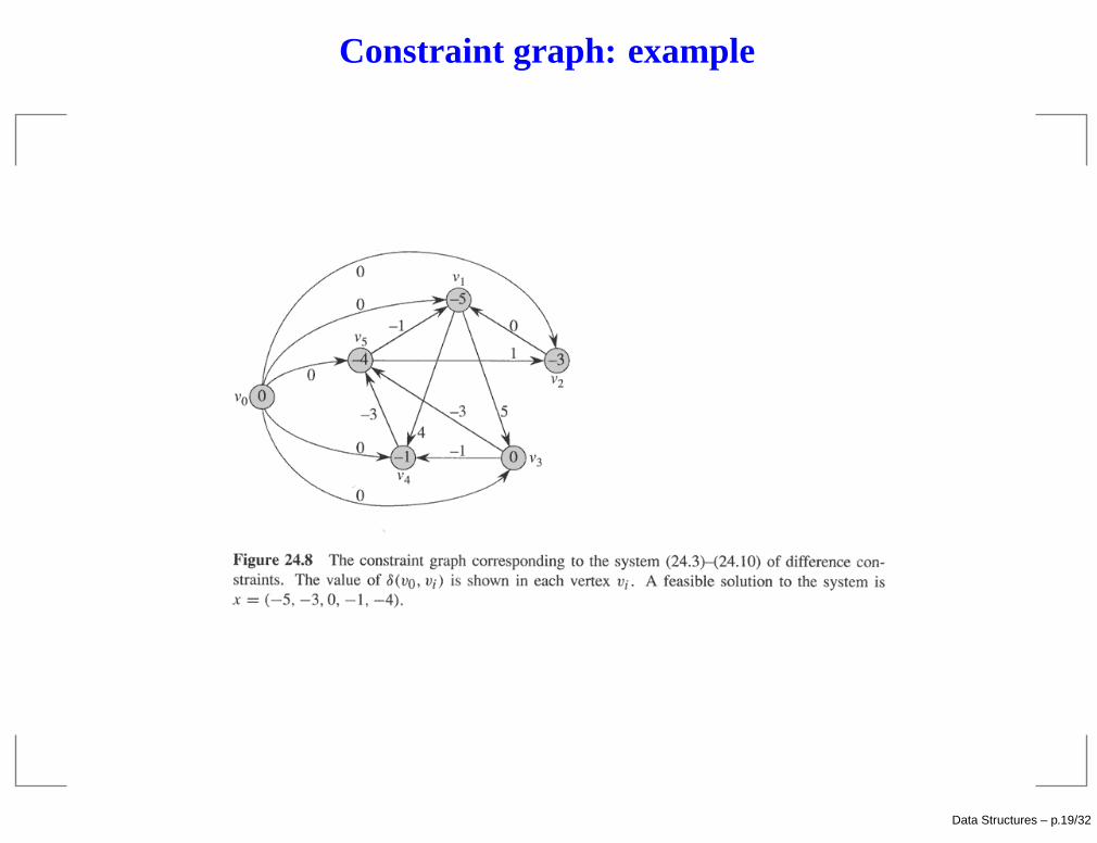
Constraint graph: example


Solving difference constraints

Theorem 1 If constraint graph has no negative-weight cycles then

(δ(v0, v1), δ(v0, v1), . . . , δ(v0, vk)),

feasible solution. If negative cycle no solution.

ALGORITHM: Bellman-Ford. m constraints on n unknowns.COMPLEXITY: graph with n + 1 vertices and n + m edges. Using Bellman-Ford can solvesystem in O((n + 1)(n + m)) = O(n2 + nm) time.


Remember: Dijkstra’s algorithm

For the case of nonnegative weights.

With good implementation lower running time than Bellman-Ford.

Maintain: set S of vertices whose shortest-path weights from the source has alreadybeen determined.

Repeatedly selects the vertex u ∈ V \ S with minimum shortest path estimate, adds u

to S and relaxes all edges leaving u.

priority queue Q of vertices, keyed by values of function d.

priority queue: data structure for maintaining a set S of elements ordered by key.

Operations: INSERT(S,x), MINIMUM(S), EXTRACT-MIN(S), INCREASE-KEY(S,x,k).

EXTRACT-MIN(S): removes and returns the element of S with the largest key.

INCREASE-KEY(S,x,x): insert the value of element x’s key to the new value k,assumed to be at least as large as x’s current key.

Implemented: min-heap.


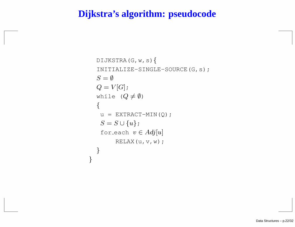
Dijkstra’s algorithm: pseudocode

DIJKSTRA(G,w,s){

INITIALIZE-SINGLE-SOURCE(G,s);

S = ∅

Q = V [G];

while (Q 6= ∅)

{

u = EXTRACT-MIN(Q);

S = S ∪ {u};

for each v ∈ Adj[u]

RELAX(u,v,w);

}

}


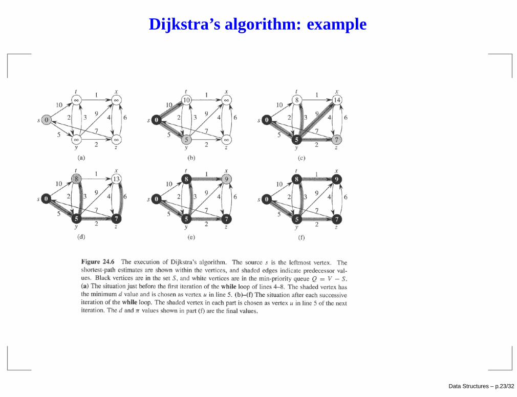
Dijkstra’s algorithm: example


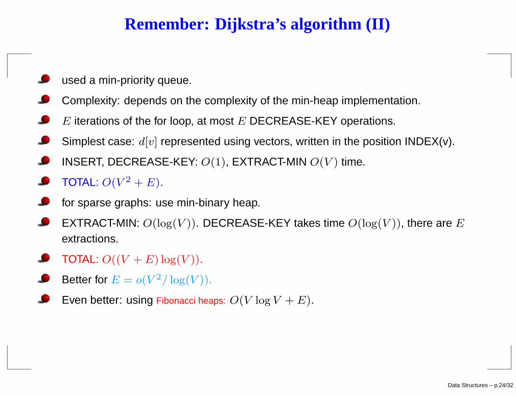
Remember: Dijkstra’s algorithm (II)

used a min-priority queue.

Complexity: depends on the complexity of the min-heap implementation.

E iterations of the for loop, at most E DECREASE-KEY operations.

Simplest case: d[v] represented using vectors, written in the position INDEX(v).

INSERT, DECREASE-KEY: O(1), EXTRACT-MIN O(V ) time.

TOTAL: O(V 2 + E).

for sparse graphs: use min-binary heap.

EXTRACT-MIN: O(log(V )). DECREASE-KEY takes time O(log(V )), there are E

extractions.

TOTAL: O((V + E) log(V )).

Better for E = o(V 2/ log(V )).

Even better: using Fibonacci heaps: O(V log V + E).


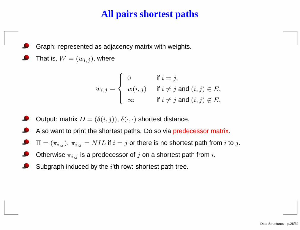
All pairs shortest paths

Graph: represented as adjacency matrix with weights.

That is, W = (wi,j), where

wi,j =

8

>

>

<

>

>

:

0 if i = j,

w(i, j) if i 6= j and (i, j) ∈ E,

∞ if i 6= j and (i, j) 6∈ E,

Output: matrix D = (δ(i, j)), δ(·, ·) shortest distance.

Also want to print the shortest paths. Do so via predecessor matrix.

Π = (πi,j). πi,j = NIL if i = j or there is no shortest path from i to j.

Otherwise πi,j is a predecessor of j on a shortest path from i.

Subgraph induced by the i’th row: shortest path tree.


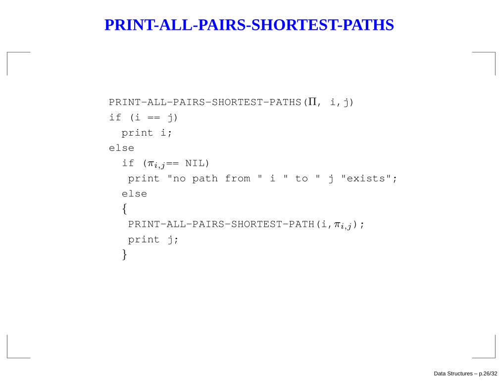
PRINT-ALL-PAIRS-SHORTEST-PATHS

PRINT-ALL-PAIRS-SHORTEST-PATHS(Π, i,j)

if (i == j)

print i;

else

if (πi,j== NIL)

print "no path from " i " to " j "exists";

else

{

PRINT-ALL-PAIRS-SHORTEST-PATH(i,πi,j);

print j;

}


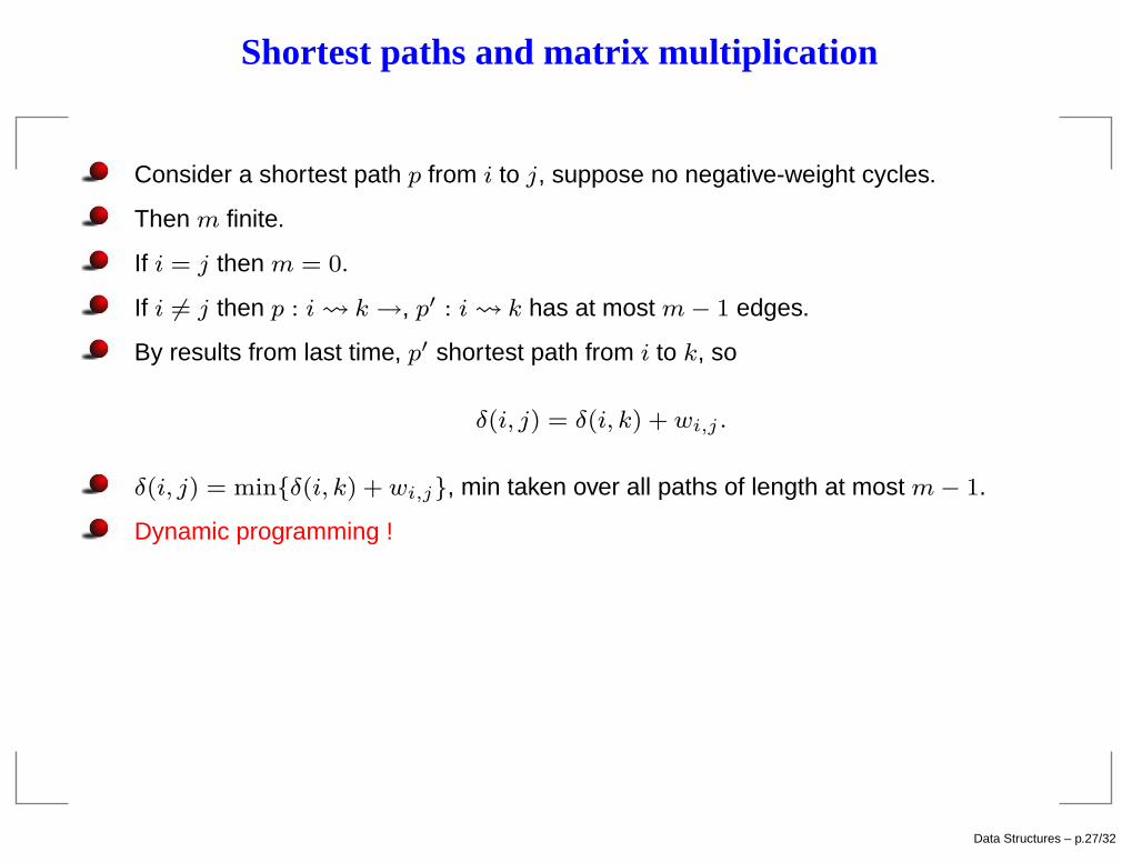
Shortest paths and matrix multiplication

Consider a shortest path p from i to j, suppose no negative-weight cycles.

Then m finite.

If i = j then m = 0.

If i 6= j then p : i k →, p′ : i k has at most m − 1 edges.

By results from last time, p′ shortest path from i to k, so

δ(i, j) = δ(i, k) + wi,j .

δ(i, j) = min{δ(i, k) + wi,j}, min taken over all paths of length at most m − 1.

Dynamic programming !


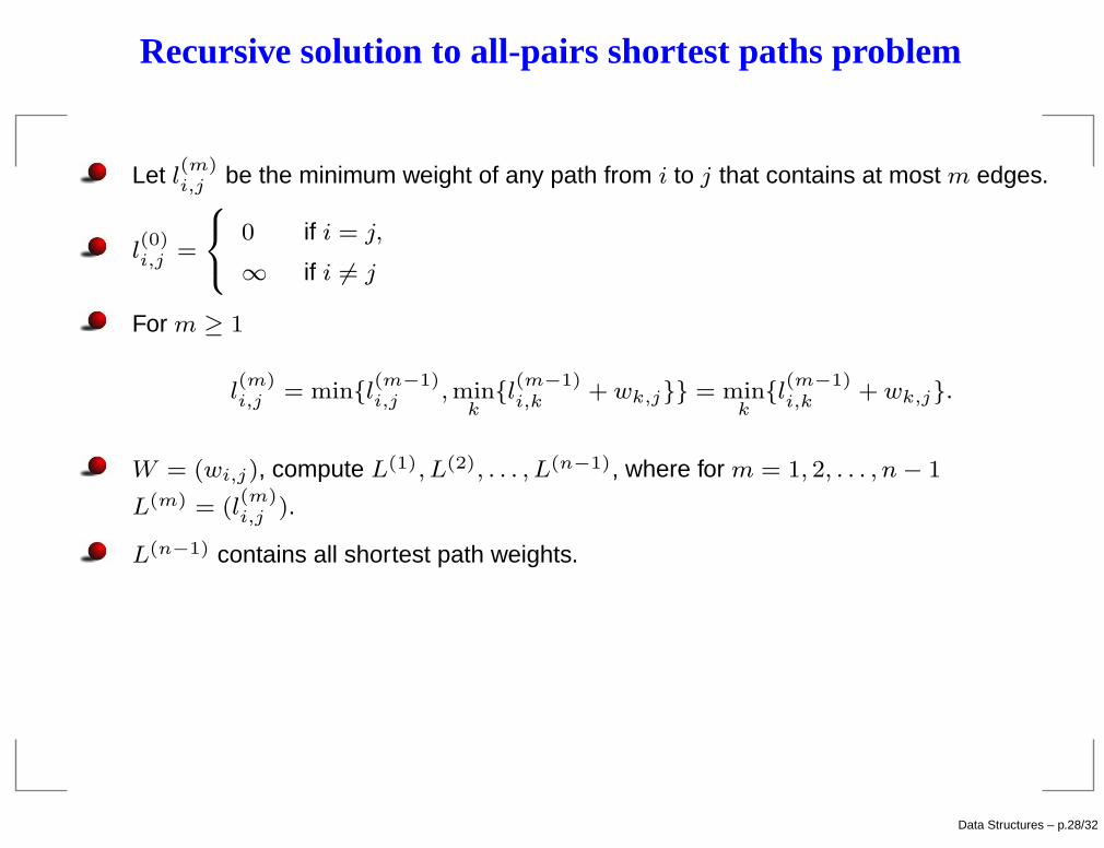
Recursive solution to all-pairs shortest paths problem

Let l(m)i,j be the minimum weight of any path from i to j that contains at most m edges.

l(0)i,j =

8

<

:

0 if i = j,

∞ if i 6= j

For m ≥ 1

l(m)i,j = min{l

(m−1)i,j , min

k{l

(m−1)i,k

+ wk,j}} = mink

{l(m−1)i,k

+ wk,j}.

W = (wi,j), compute L(1), L(2), . . . , L(n−1), where for m = 1, 2, . . . , n − 1

L(m) = (l(m)i,j ).

L(n−1) contains all shortest path weights.


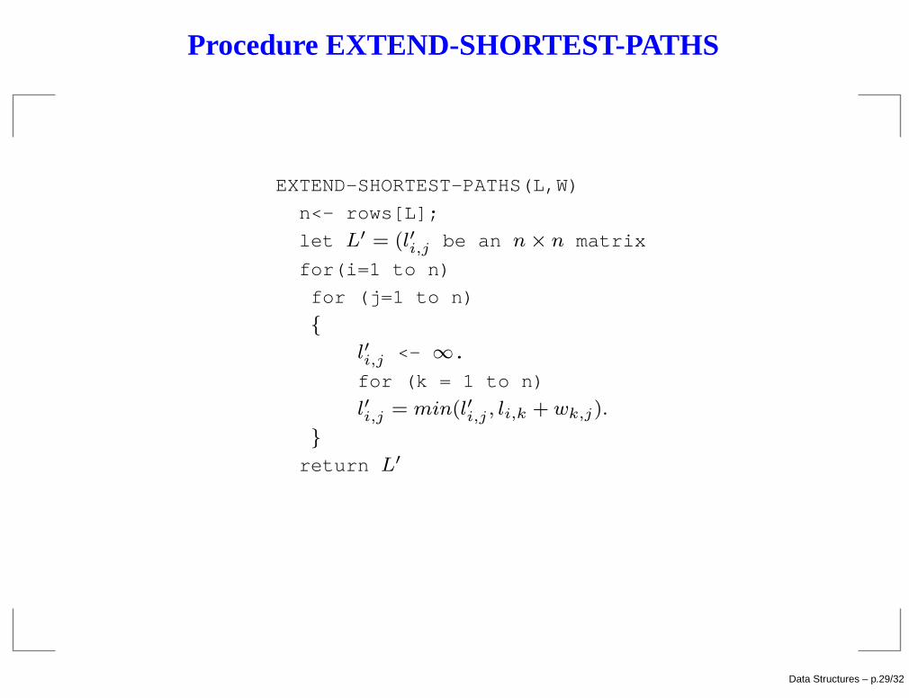
Procedure EXTEND-SHORTEST-PATHS

EXTEND-SHORTEST-PATHS(L,W)

n<- rows[L];

let L′ = (l′i,j be an n × n matrix

for(i=1 to n)

for (j=1 to n)

{

l′i,j <- ∞.

for (k = 1 to n)

l′i,j = min(l′i,j , li,k + wk,j).

}

return L′


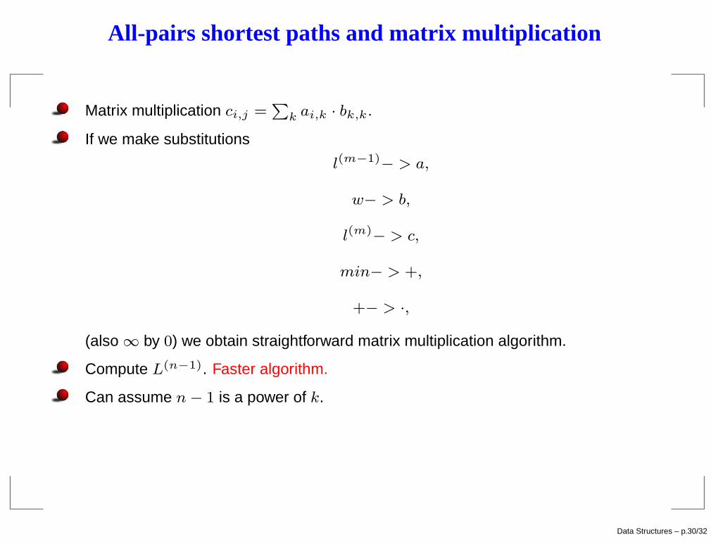
All-pairs shortest paths and matrix multiplication

Matrix multiplication ci,j =P

k ai,k · bk,k.

If we make substitutions

l(m−1)− > a,

w− > b,

l(m)− > c,

min− > +,

+− > ·,

(also ∞ by 0) we obtain straightforward matrix multiplication algorithm.

Compute L(n−1). Faster algorithm.

Can assume n − 1 is a power of k.


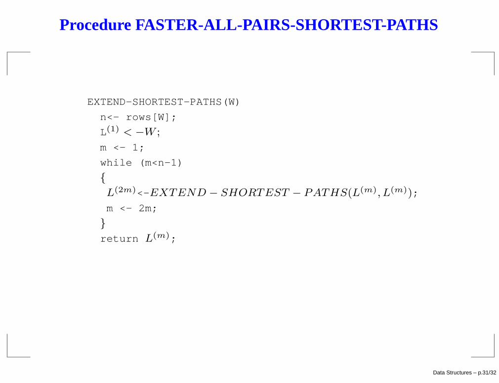
Procedure FASTER-ALL-PAIRS-SHORTEST-PATHS

EXTEND-SHORTEST-PATHS(W)

n<- rows[W];

L(1) < −W ;

m <- 1;

while (m<n-1)

{

L(2m)<-EXTEND − SHORTEST − PATHS(L(m), L(m));

m <- 2m;

}

return L(m);


Conclusions

Please ask questions if you don’t understand something!

Newsgroup for questions: adsuvt2007.

Any questions ?


single sourse shortest paths: formulation - gabriel...

Documents