sistema de amplificaciÓn para dispositivos...
TRANSCRIPT
PONTIFICIA UNIVERSIDAD CATOLICA DE CHILE
ESCUELA DE INGENIERIA
SISTEMA DE AMPLIFICACIÓN PARA
DISPOSITIVOS DISTRIBUIDOS DE
DISIPACIÓN DE ENERGÍA
JUAN SEBASTIÁN BAQUERO MOSQUERA
Tesis para optar al grado de
Magister en Ciencias de la Ingeniería
Profesor Supervisor:
JOSE LUIS ALMAZÁN CAMPILLAY, PH.D.
Santiago de Chile, Mayo 2015
MMXV, Juan Sebastián Baquero Mosquera
PONTIFICIA UNIVERSIDAD CATOLICA DE CHILE
ESCUELA DE INGENIERIA
SISTEMA DE AMPLIFICACIÓN PARA
DISPOSITIVOS DISTRIBUIDOS DE
DISIPACIÓN DE ENERGÍA
JUAN SEBASTIÁN BAQUERO MOSQUERA
Tesis presentada a la Comisión integrada por los profesores:
JOSE LUIS ALMAZÁN CAMPILLAY, PH.D.
MATÍAS HUBE GINESTAR, PH.D.
JUAN FELIPE BELTRÁN, PH.D.
RODRIGO ESCOBAR MORAGAS, PH.D.
Para completar las exigencias del grado de
Magister en Ciencias de la Ingeniería
Santiago de Chile, Mayo 2015

ii
A Patricio Baquero y María Teresa
Mosquera, María José y Salomé
Baquero, Emilia y Martina. Mi
incondicional familia y el motor que
impulsa cada anhelo y meta
planteados.

iii
AGRADECIMIENTOS
A Dios, por la oportunidad de vivir esta experiencia enriquecedora y culminar la meta
planteada. A mi Papá, Mamá, hermanas y mis enanitas, gracias a su apoyo incondicional y
su amor he dado cada paso desde que comencé este camino. A "La Legión'', amigos y
hermanos que la causa puso a mi lado para compartir y combatir fuera de casa.
A la Secretaria Nacional de Educación Superior, Ciencia, Tecnología e Innovación,
SENESCYT, por el apoyo brindado por medio de la convocatoria abierta de becas. Sin su
ayuda no habría sido posible el iniciar mis estudios en el Programa de Maestrías.
Este documento y el contenido en el que se basa, ha sido posible gracias a la guía y paciencia
de mi Profesor Tutor José Luis Almazán, quien ha sabido proponer de manera adecuada los
pasos por recorrer a lo largo de ésta investigación. A la valiosa colaboración de Yoslandy
Lazo y del Laboratorio del Departamento de Ingeniería Estructural y Geotécnica, a su
personal del DICTUC: Nicolás Tapia Atilio Muñoz y sus colaboradores, a José Luis Ramírez
de la empresa ARIES - Ingeniería y Sistemas, por su intenso trabajo y capacitación del equipo
pseudo-dinámico, y finalmente a la no menos importante ayuda de los profesores parte del
Comité, quienes con su tiempo y experiencia han ayudado a mejorar en forma y fondo el
texto que se expone en adelante.
INDICE GENERAL
Pág.
DEDICATORIA ...................................................................................................... ii
AGRADECIMIENTOS .......................................................................................... iii
INDICE DE TABLAS ............................................................................................ vi
INDICE DE FIGURAS .......................................................................................... vii
RESUMEN ...............................................................................................................x
ABSTRACT .......................................................................................................... xii
1. INTRODUCCIÓN ...........................................................................................1
2. SISTEMA DE AMPLIFICACIÓN PROPUESTO ............................................4
2.1. Factor de Amplificación Teórico. .............................................................5
3. MODELO DE UN PISO 2D – 1 GRADO DE LIBERTAD (1GDL) ................6
3.1. Modelo sin Sistema de Amplificación ......................................................6
3.2. Modelo con Sistema de Amplificación LAS o ELAS ............................. 10
4. MODELO DE MÚLTIPLES GRADOS DE LIBERTAD ............................... 16
4.1. Modelo de Edificio de 7 Pisos ................................................................ 16
4.2. Modelo de Edificio de 5 pisos. Sistema Dual (Muro-Pórtico) ................. 24
5. ESTUDIO EXPERIMENTAL ....................................................................... 30
5.1. Espécimen de Prueba e instalación del mecanismo ELAS ...................... 30
5.2. Amortiguador Friccional ........................................................................ 34
5.3. Ensayo Pseudo-Dinámico ...................................................................... 35
5.3.1. Ensayos con excitación sísmica.................................................... 38
6. CONCLUSIONES ......................................................................................... 45
BIBLIOGRAFIA .................................................................................................... 47

A N E X O S ........................................................................................................... 50
ANEXO A: CÁLCULO DEL FACTOR DE AMPLIFICACIÓN TEÓRICA ........... 51
ANEXO B: PUBLICACIÓN PRESENTADA N.1 .................................................. 52
ANEXO C: PUBLICACIÓN PRESENTADA N. 2 ................................................. 53

vi
INDICE DE TABLAS
Pág.
Tabla 4- 1: Número de Unidades necesarias ................................................................. 20
Tabla 4- 2: Propiedades Estructurales. Modelo de Sistema dual de 5 pisos. .................. 27
Tabla 4- 3: Respuesta del sistema dual de 5 Pisos. ....................................................... 29
vii
INDICE DE FIGURAS
Pág.
Figura 1- 1: Representación esquemática de: (a) y (b) configuraciones convencionales;
y, (c)-(f) mecanismos de amplificación existentes. ......................................................... 3
Figura 2- 1: Eccentric Lever-Arm System (ELAS); (a) 1 amortiguador (Disipación
Concentrada); y (b) múltiples amortiguadores (Disipación Distribuida) ......................... 5
Figura 3- 1: Modelo esquemático de un sistema 1 GDL con amortiguamiento
suplementario. ............................................................................................................... 8
Figura 3- 2: Efectos del amortiguamiento suplementario d y la relación de rigideces
kd/ks para una estructura con s = y s = 0; (a) Factor de amortiguamiento
efectivo deff; y (b) desviación estándar normalizada para el desplazamiento estructural
qt (en línea llena), y la deformación del soporte z(t) (línea cortada). ............................. 9
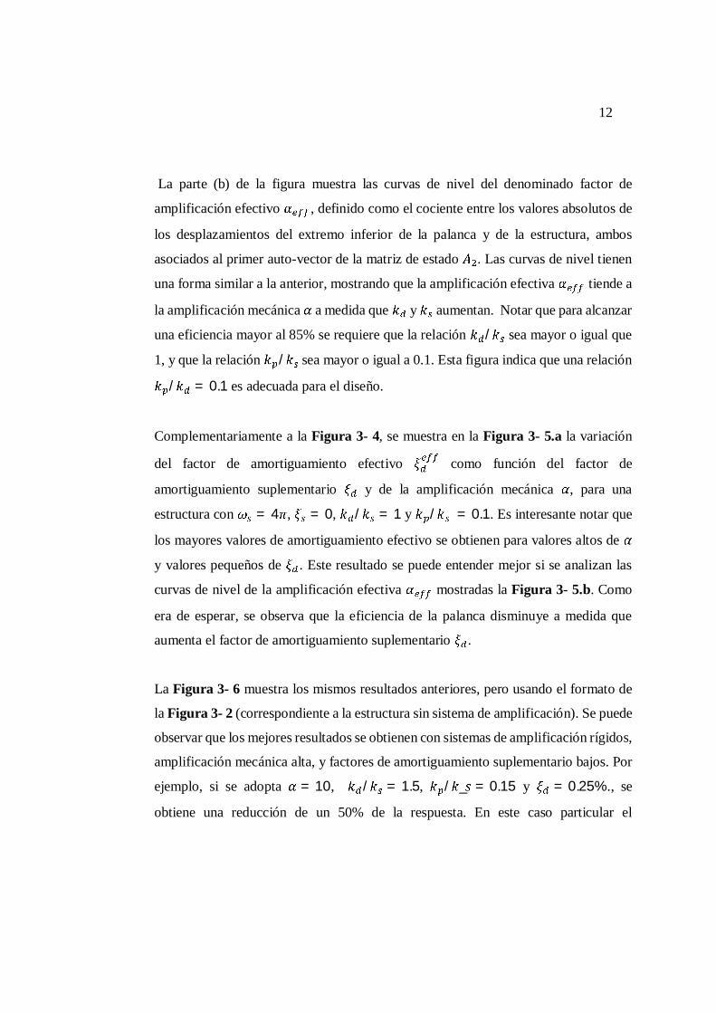
Figura 3- 3: Modelo esquemático de un sistema de 1 GDL con mecanismo LAS y
amortiguamiento suplementario. .................................................................................. 13
Figura 3- 4: Análisis de Sensibilidad de un Sistema de 1 GDL acoplado con mecanismo
LAS usando: = 10; add = 2/1000; a) mostrando la superficie de amortiguamiento
efectivo deff, y; b) factor de amplificación efectiva eff, ambos mientras varia l. ..... 14
Figura 3- 5: Análisis de Sensibilidad de un Sistema de 1 GDL acoplado con mecanismo
LAS usando: d = 1, p = 0.1; a) mostrando la superficie de amortiguamiento efectivo
deff, y; b) factor de amplificación efectiva eff, ambos mientras varia el
amortiguamiento suplementario add. ......................................................................... 14
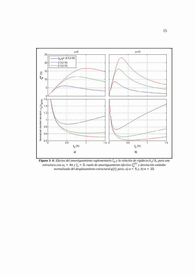
Figura 3- 6: Efectos del amortiguamiento suplementario d y la relación de rigideces
kd/ks para una estructura con s = y s = 0, razón de amortiguamiento efectivo
deff y desviación estándar normalizada del desplazamiento estructural q(t) para; a)
= 5 y, b) = 10. ..................................................................................................... 15
viii
Figura 4- 1: a) Modelo Estructural y sus propiedades; b) configuración convencional
con chevron; c) configuración convencional con diagonales; d) configuración con
mecanismo LAS; y e) configuración con mecanismo ELAS (propuesto). ..................... 18
Figura 4- 2: Drift de piso después de hacer la distribución en altura de los dispositivos
de disipación usando el método SSSA. ........................................................................ 22
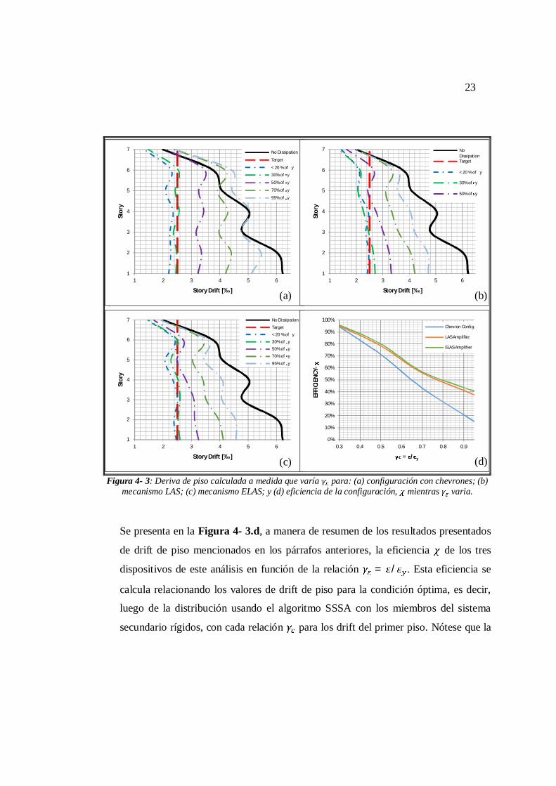
Figura 4- 3: Deriva de piso calculada a medida que varía para: (a) configuración con
chevrones; (b) mecanismo LAS; (c) mecanismo ELAS; y (d) eficiencia de la
configuración, mientras varia. .............................................................................. 23
Figura 4- 4: Modelo estructural del sistema dual analizado. ........................................ 26
Figura 4- 5: Historia de energía disipada en el sistema. ............................................... 27
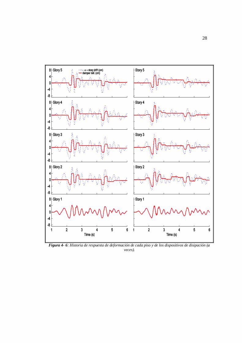
Figura 4- 6: Historia de respuesta de deformación de cada piso y de los dispositivos de
disipación ( veces). .................................................................................................... 28
Figura 5- 1: Espécimen de prueba, vista general. ......................................................... 31
Figura 5- 2: Planta general y detalles de columnas, bases y vigas perimetrales. ........... 32
Figura 5- 3: Espécimen de prueba sobre losa de reacción y acoplado al equipo pseudo-
dinámico. ..................................................................................................................... 33
Figura 5- 4: Esquema del mecanismo de Amplificación e instalación en el pórtico
exterior del espécimen de prueba. ................................................................................ 33
Figura 5- 5: Esquema del disipador friccional e instalación en el conjunto amplificador
(ELAS)-estructura. ...................................................................................................... 35
Figura 5- 6: Disposición de ensayos Pseudo-Dinámicos. ............................................. 38
Figura 5- 7: Historia de aceleraciones N-S del registro El Centro, y; Espectro de
respuesta elástica, registro original y artificial (ART). .................................................. 39
Figura 5- 8: Comparación desplazamientos en los bordes sin disipador (arriba) y con
disipador (abajo). Registro escalado al 30%, excentricidad e=100 cm. ......................... 41
ix
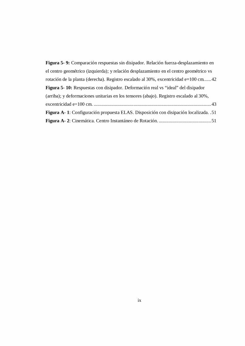
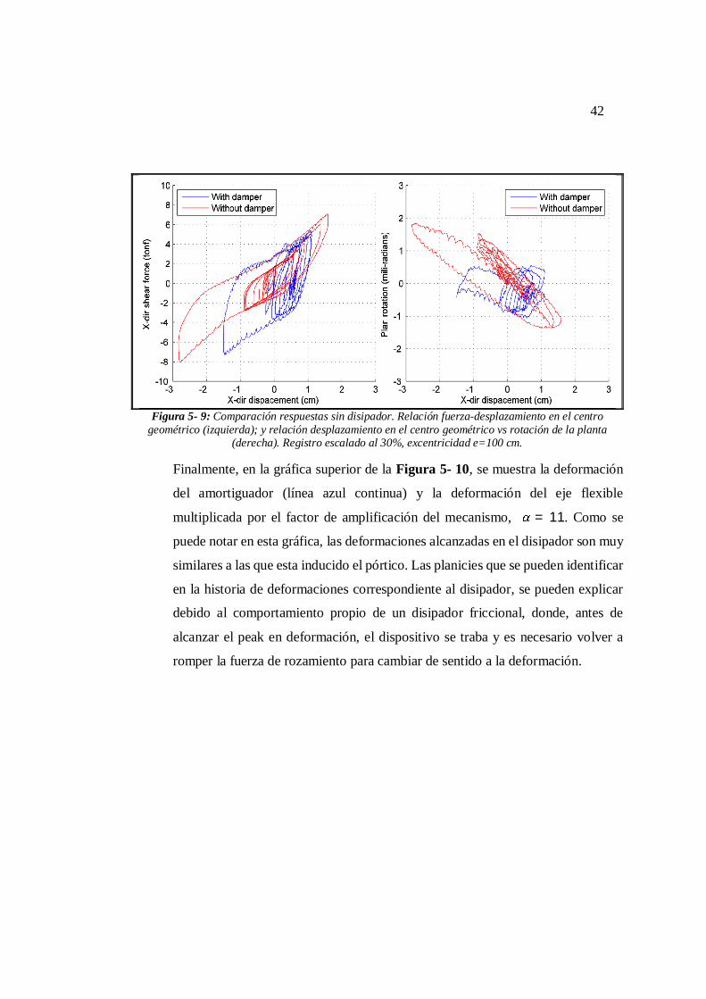
Figura 5- 9: Comparación respuestas sin disipador. Relación fuerza-desplazamiento en
el centro geométrico (izquierda); y relación desplazamiento en el centro geométrico vs
rotación de la planta (derecha). Registro escalado al 30%, excentricidad e=100 cm...... 42
Figura 5- 10: Respuestas con disipador. Deformación real vs “ideal” del disipador
(arriba); y deformaciones unitarias en los tensores (abajo). Registro escalado al 30%,
excentricidad e=100 cm. .............................................................................................. 43
Figura A- 1: Configuración propuesta ELAS. Disposición con disipación localizada. . 51
Figura A- 2: Cinemática. Centro Instantáneo de Rotación. .......................................... 51
x
RESUMEN
En las últimas dos décadas aproximadamente, se han venido realizando estudios de
carácter analítico, experimental y de aplicación a sistemas de protección dinámica que
utilizan dispositivos de disipación de energía ya sean activos o pasivos, para mejorar el
desempeño de diversas estructuras ante eventos de tipo dinámico. Estos eventos pueden
ser de origen sísmico o por efectos de presión de viento.
Los dispositivos de disipación de energía aprovechan generalmente los desplazamientos
de entrepiso y las velocidades derivadas de estos desplazamientos para entrar en
funcionamiento. Por lo tanto, será obvio notar que para una configuración estructural
relativamente flexible, estas respuestas de la estructura serán mejor aprovechadas por los
disipadores de energía que las respuestas inducidas por los eventos dinámicos en una
estructura más rígida. Las limitaciones de Normas de diseño y construcción
correspondientes a las deformaciones admisibles en un sistema estructural, también
pueden ser consideradas como restricciones a las respuestas de las que toman ventajas los
sistemas de protección sísmica.
En función de estas consideraciones, se han propuesto, probado y patentado varios
mecanismos de amplificación de desplazamientos como los de (Hetrick & Kota, 2003) y
(Berton, 2004). Estos mecanismos, conocidos como DAD por sus siglas en inglés
(Displacement Amplification Devices), son ensambles de miembros idealmente rígidos
que debido a su disposición geométrica y cinemática generan ventaja mecánica en fuerza
y desplazamiento (traducida en amplificación de estos efectos) de un punto a otro de dicho
ensamble. Los más estudiados de estos mecanismos han sido los de tipo lever-arm, que
emplean la teoría de apalancamiento para generar la amplificación ya mencionada.

xi
En esta investigación se presenta y pone a prueba experimental y analítica, un dispositivo
de amplificación de desplazamientos que por su disposición geométrica y cinemática, es
considerado como novedoso. En el documento se expone inicialmente un análisis del
comportamiento del DAD propuesto, demostrando teóricamente su funcionamiento y
factores de amplificación que es posible alcanzar con éste. Además, se generan modelos
estructurales matemáticos, en los cuales se implementa el mecanismo para llegar a una
primera aproximación de la eficiencia de este DAD y comparación con otros existentes.
Finalmente, se somete a prueba experimental por medio de ensayos Pseudo – Dinámicos
aplicados a una estructura de prueba a escala real con dos tipos de disipadores, uno
friccional (Montaño, 2015) y otro histerético auto-centrante (Tapia Flores, 2015), con el
fin de determinar la eficiencia real y establecer las posibles causas de pérdida de eficiencia
que existiría en un caso de aplicación real.
Finalmente, por medio de la evaluación experimental, se ratifica de manera satisfactoria
que lo obtenido de la evaluación analítica es consistente con un análisis de caso real y que
el mecanismo de amplificación propuesto cumple con la función para cual fue concebido.
Palabras clave:
Sistema de protección sísmica, dispositivo de disipación de energía, respuesta estructural,
dispositivo/mecanismo de amplificación de desplazamientos, configuración cinemática,
factor de amplificación, ensayo pseudo-dinámico.
xii
ABSTRACT
Lately, there have been made several analytic, experimental and real practice studies to
seismic protection systems which use both active and passive energy dissipation devices,
combined with other mechanisms to enhance the structural behavior against dynamic
events originated by earthquakes or wind pressure.
These devices take advantage of the inter-story displacements and velocities induced by
the structural response to start working. Hence, it’s obvious to notice that for a relatively
flexible structural configuration, these structural responses will be better used by the
energy dissipation devices than those induced in a rigid one. Based on these
considerations, mechanisms known as DAD (Displacement Amplification Devices ),
which main purpose is to improve the efficiency of the energy dissipation devices, -
especially those installed in rigid structures- have been proposed, tested and patented
(Hetrick & Kota, 2003) and (Berton, 2004).
This research presents and tests in an experimental and analytic manner, a novel geometric
and cinematic configuration for a lever-arm type DAD. First an analysis of its cinematic
behavior is exposed, demonstrating its theoretical functioning and suitable amplification
factors. Then, mathematical models are generated and used to introduce the proposed
DAD, evaluate its initial efficiency and compare with other mechanisms of the same type.
Finally, it’s experimentally tested, coupled to two types of energy dissipation devices; one
frictional (Montaño, 2015), and the other one histeretical (Tapia Flores, 2015), with a
pseudo-dynamic equipment in order to determine the real efficiency and establish possible
causes of efficiency losses in a real-scenario application case.

xiii
Finally, by means of this experimental evaluation, it could be successfully ratified that
those analytical evaluation results and conclusions are consistent with a real case
simulated scenario. Hence, the amplification mechanism here proposed is suitable to its
purpose.
Keywords:
Seismic protection system, dissipation device, structural response, displacement
amplification system/mechanism, cinematic configuration, amplification factor,
mechanism efficiency, pseudo-dynamic test.

1
1. INTRODUCCIÓN
Cada vez es más frecuente la utilización de dispositivos de protección sísmica dedicados
a la disipación de energía de estructuras civiles. Estos dispositivos se pueden clasificar
como: viscosos, visco-elásticos, metálicos y friccionales (Symans et al., 2008). En
edificios, por ejemplo, estos dispositivos aprovechan la deformación de entrepiso para
activarse y disipar energía. Su instalación se realiza según dos configuraciones típicas: (i)
el disipador trabaja en sentido horizontal conectando la viga con una estructura auxiliar
formada por dos elementos metálicos que forman una V invertida (chevron); y (ii) el
disipador trabaja en forma oblicua (diagonal) conectando directamente las uniones viga-
columna (nodos) de la estructura (Constantinou, Tsopelas, Hammel, & Sigaher, 2001) y
(Aiken, Nims, Whittaker, & Kelly, 1993). Aunque el sistema diagonal es evidentemente
más simple, sólo es capaz de aprovechar una fracción de la deformación de entrepiso.
En estructuras flexibles ambas configuraciones resultan en general apropiadas. Sin
embargo, para estructuras rígidas como los edificios construidos con muros de hormigón
armado en los que se producen pequeñas deformaciones de entrepiso, la implementación
de sistemas de disipación de energía resulta más difícil y muchas veces impracticable.
Para solucionar este inconveniente se han propuesto sistemas que combinan dispositivos
de disipación de energía con mecanismos de amplificación de deformaciones o
simplemente se han realizado análisis de tipo experimental ante la existencia de esta
amplificación de deformaciones para ser aprovechadas por los dispositivos de disipación
de energía (Londoño, Neild, & Wagg, 2015). Por ejemplo, el sistema denominado
“Toggle-Brace Damper” (TBD) (Constantinou et al., 2001) es capaz de alcanzar
amplificaciones de desplazamiento entre 2 y 3. Se han propuesto también sistemas de
amplificación en base a piñones de distinto diámetro (Berton & Bolander, 2005), sistemas
2
tipo lever-arm (Ribakov & Reinhorn, 2003), y dispositivos de amplificación hidráulica
(Chung & Lam, 2004). Estudios experimentales y analíticos de algunos de estos
mecanismos muestran que los valores viables de amplificación varían entre 2 y 8 (Berton
& Bolander, 2005) y (Ribakov & Reinhorn, 2003).
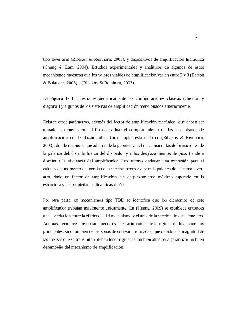
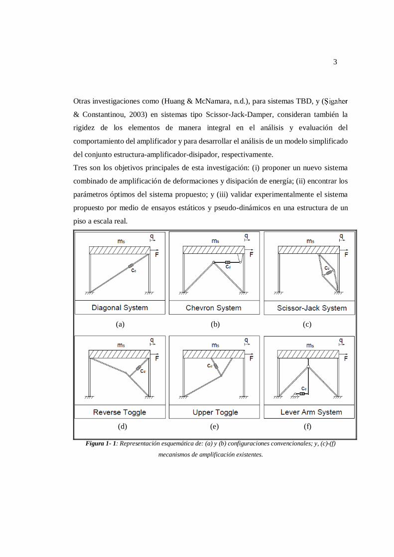
La Figura 1- 1 muestra esquemáticamente las configuraciones clásicas (chevron y
diagonal) y algunos de los sistemas de amplificación mencionados anteriormente.
Existen otros parámetros, además del factor de amplificación mecánico, que deben ser
tomados en cuenta con el fin de evaluar el comportamiento de los mecanismos de
amplificación de desplazamientos. Un ejemplo, está dado en (Ribakov & Reinhorn,
2003), donde reconoce que además de la geometría del mecanismo, las deformaciones de
la palanca debido a la fuerza del disipador y a los desplazamientos de piso, tiende a
disminuir la eficiencia del amplificador. Los autores deducen una expresión para el
cálculo del momento de inercia de la sección necesaria para la palanca del sistema lever-
arm, dado un factor de amplificación, un desplazamiento máximo esperado en la
estructura y las propiedades dinámicas de ésta.
Por otra parte, en mecanismos tipo TBD se identifica que los elementos de este
amplificador trabajan axialmente únicamente. En (Huang, 2009) se establece entonces
una correlación entre la eficiencia del mecanismo y el área de la sección de sus elementos.
Además, reconoce que no solamente es necesario cuidar de la rigidez de los elementos
principales, sino también de las zonas de conexión rotuladas, que debido a la magnitud de
las fuerzas que se transmiten, deben tener rigideces también altas para garantizar un buen
desempeño del mecanismo de amplificación.
3
Otras investigaciones como (Huang & McNamara, n.d.), para sistemas TBD, y (
& Constantinou, 2003) en sistemas tipo Scissor-Jack-Damper, consideran también la
rigidez de los elementos de manera integral en el análisis y evaluación del
comportamiento del amplificador y para desarrollar el análisis de un modelo simplificado
del conjunto estructura-amplificador-disipador, respectivamente.
Tres son los objetivos principales de esta investigación: (i) proponer un nuevo sistema
combinado de amplificación de deformaciones y disipación de energía; (ii) encontrar los
parámetros óptimos del sistema propuesto; y (iii) validar experimentalmente el sistema
propuesto por medio de ensayos estáticos y pseudo-dinámicos en una estructura de un
piso a escala real.
(a) (b) (c)
(d) (e) (f)
Figura 1- 1: Representación esquemática de: (a) y (b) configuraciones convencionales; y, (c)-(f)
mecanismos de amplificación existentes.
4
2. SISTEMA DE AMPLIFICACIÓN PROPUESTO
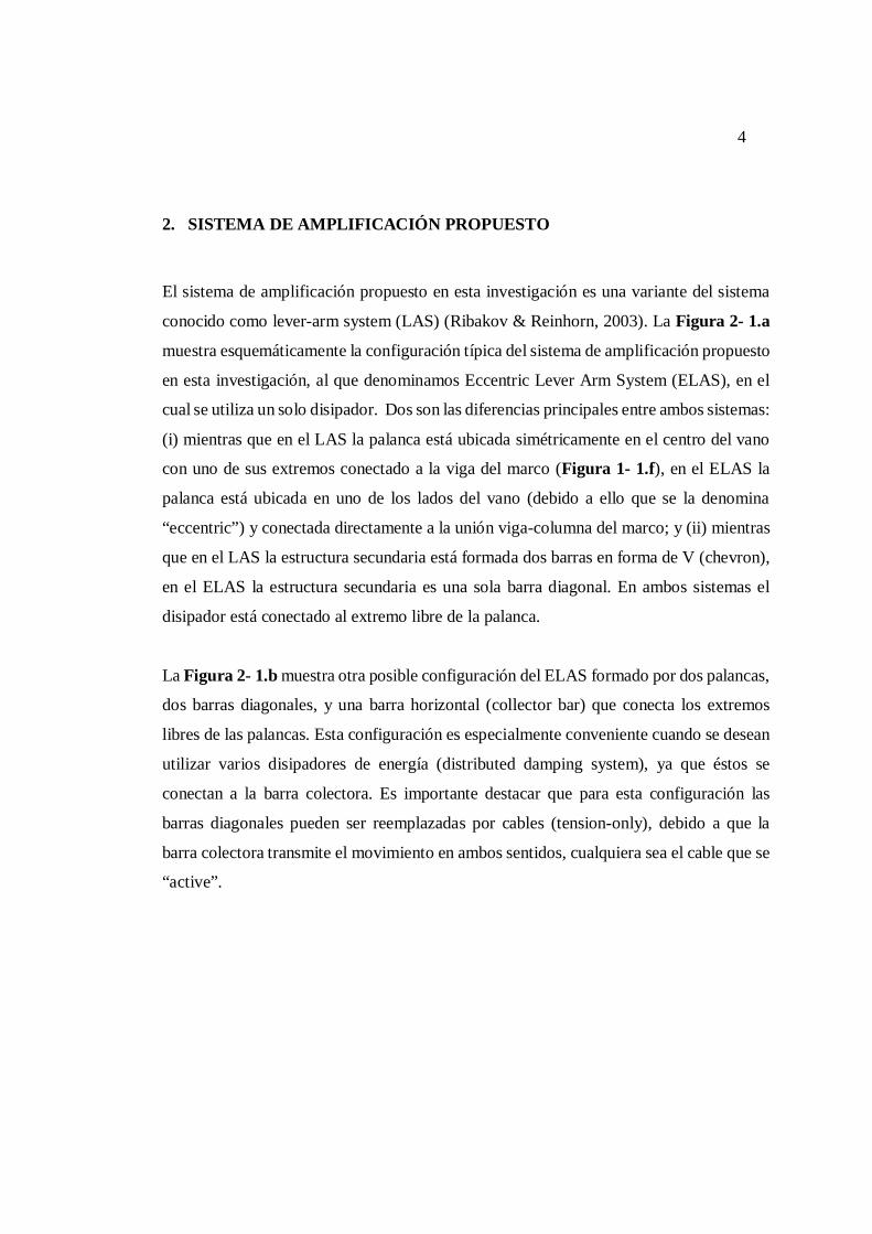
El sistema de amplificación propuesto en esta investigación es una variante del sistema
conocido como lever-arm system (LAS) (Ribakov & Reinhorn, 2003). La Figura 2- 1.a
muestra esquemáticamente la configuración típica del sistema de amplificación propuesto
en esta investigación, al que denominamos Eccentric Lever Arm System (ELAS), en el
cual se utiliza un solo disipador. Dos son las diferencias principales entre ambos sistemas:
(i) mientras que en el LAS la palanca está ubicada simétricamente en el centro del vano
con uno de sus extremos conectado a la viga del marco (Figura 1- 1.f), en el ELAS la
palanca está ubicada en uno de los lados del vano (debido a ello que se la denomina
“eccentric”) y conectada directamente a la unión viga-columna del marco; y (ii) mientras
que en el LAS la estructura secundaria está formada dos barras en forma de V (chevron),
en el ELAS la estructura secundaria es una sola barra diagonal. En ambos sistemas el
disipador está conectado al extremo libre de la palanca.
La Figura 2- 1.b muestra otra posible configuración del ELAS formado por dos palancas,
dos barras diagonales, y una barra horizontal (collector bar) que conecta los extremos
libres de las palancas. Esta configuración es especialmente conveniente cuando se desean
utilizar varios disipadores de energía (distributed damping system), ya que éstos se
conectan a la barra colectora. Es importante destacar que para esta configuración las
barras diagonales pueden ser reemplazadas por cables (tension-only), debido a que la
barra colectora transmite el movimiento en ambos sentidos, cualquiera sea el cable que se
“active”.
5
a
a Figura 2- 1: Eccentric Lever-Arm System (ELAS); (a) 1 amortiguador (Disipación Concentrada); y (b)
múltiples amortiguadores (Disipación Distribuida)
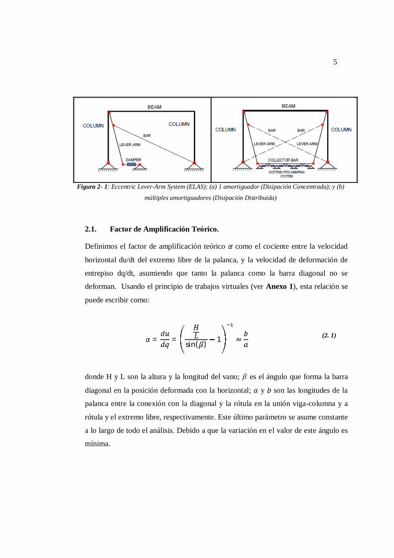
2.1. Factor de Amplificación Teórico.
Definimos el factor de amplificación teórico como el cociente entre la velocidad
horizontal du/dt del extremo libre de la palanca, y la velocidad de deformación de
entrepiso dq/dt, asumiendo que tanto la palanca como la barra diagonal no se
deforman. Usando el principio de trabajos virtuales (ver Anexo 1), esta relación se
puede escribir como:
= = sin( ) 1 (2. 1)
donde H y L son la altura y la longitud del vano; es el ángulo que forma la barra
diagonal en la posición deformada con la horizontal; y son las longitudes de la
palanca entre la conexión con la diagonal y la rótula en la unión viga-columna y a
rótula y el extremo libre, respectivamente. Este último parámetro se asume constante
a lo largo de todo el análisis. Debido a que la variación en el valor de este ángulo es
mínima.
6
3. MODELO DE UN PISO 2D – 1 GRADO DE LIBERTAD (1GDL)
Diversos investigadores han señalado que la rigidez del sistema secundario tiene gran
influencia en la eficiencia del sistema de disipación implementado (Ribakov & Reinhorn,
2003), (Huang & McNamara, n.d.). y (Huang, 2004).
Esta influencia es aún más importante cuando se utilizan dispositivos de amplificación de
deformaciones, debido a la mayor complejidad del sistema secundario.
Como paso previo al estudio de sistemas de múltiples grados de libertad, se analiza en
esta sección una estructura de 1GDL con amortiguamiento suplementario de tipo viscoso
lineal. Se consideran dos casos: (a) sin sistema de amplificación; y (b) con sistema de
amplificación de tipo lever-arm.
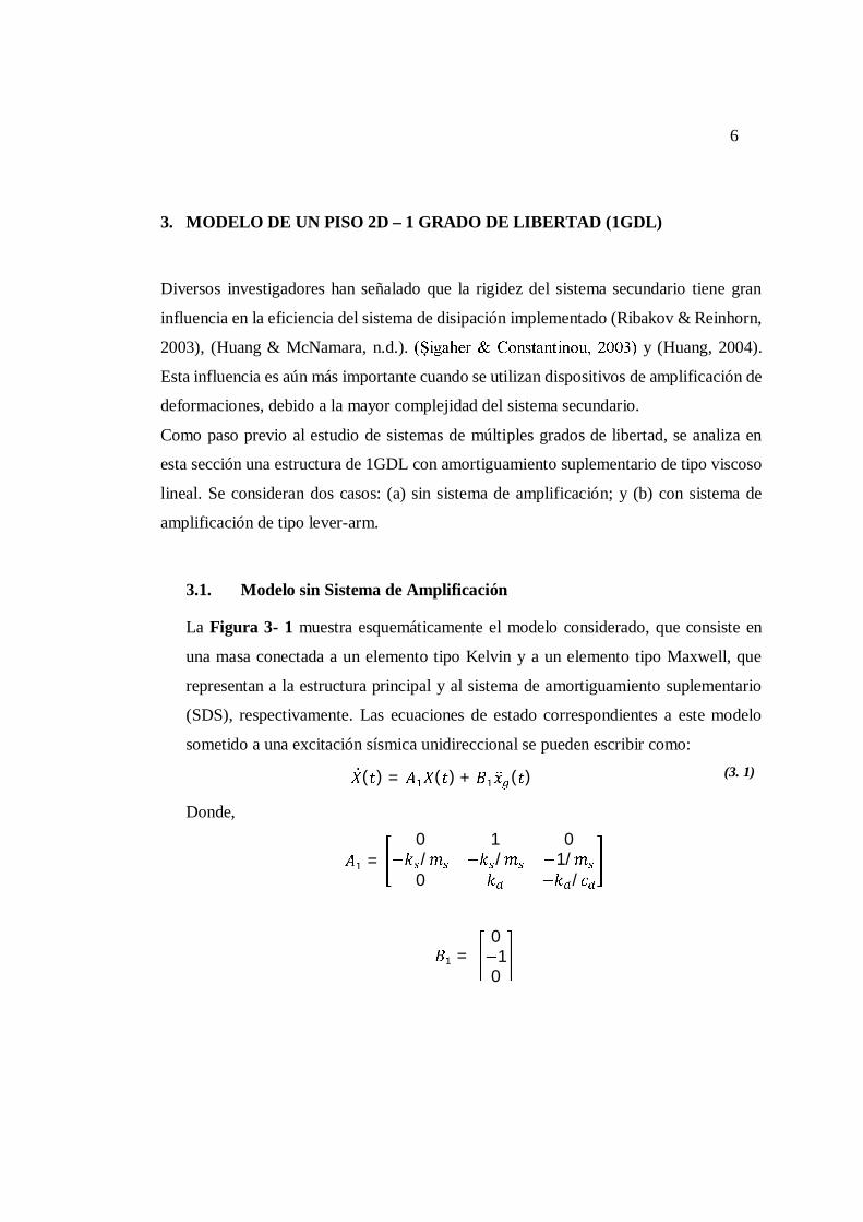
3.1. Modelo sin Sistema de Amplificación
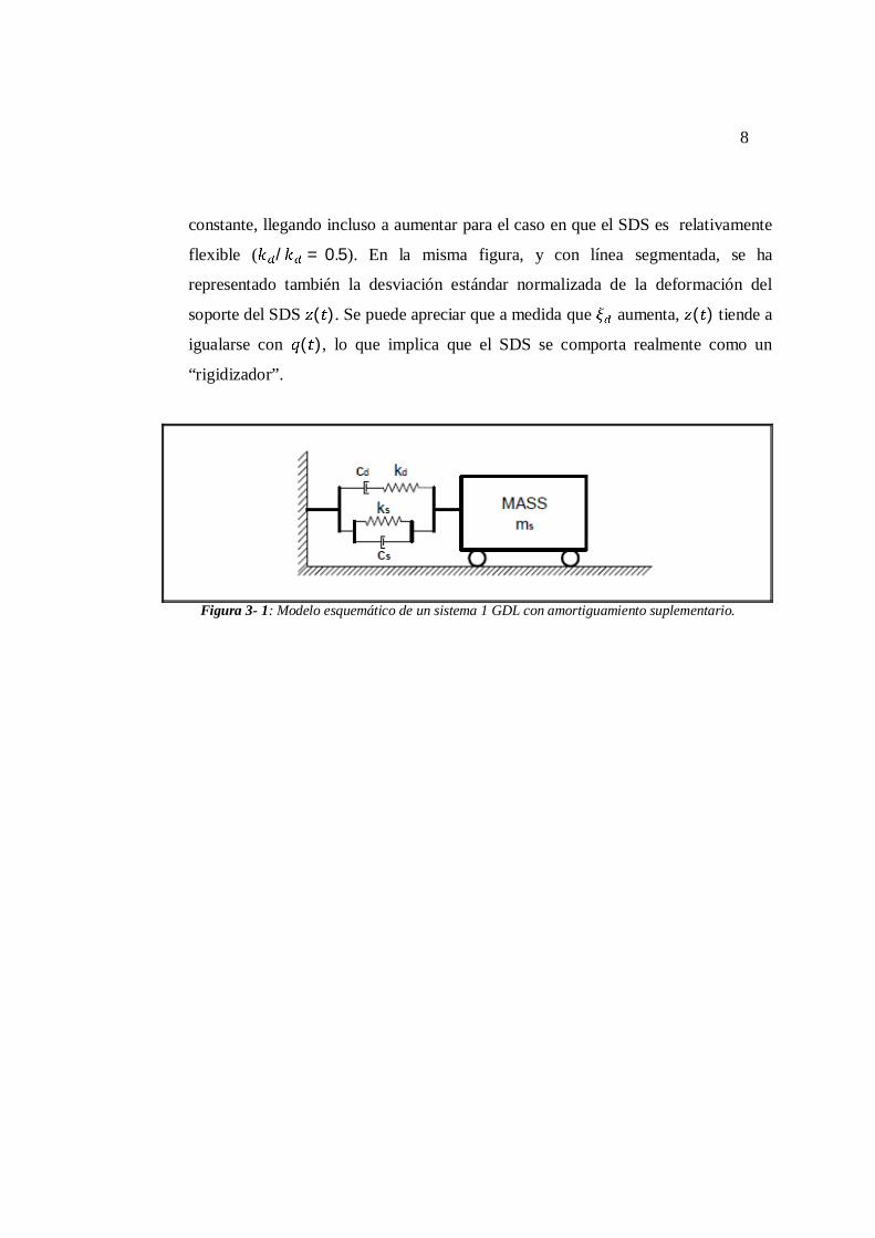
La Figura 3- 1 muestra esquemáticamente el modelo considerado, que consiste en
una masa conectada a un elemento tipo Kelvin y a un elemento tipo Maxwell, que
representan a la estructura principal y al sistema de amortiguamiento suplementario
(SDS), respectivamente. Las ecuaciones de estado correspondientes a este modelo
sometido a una excitación sísmica unidireccional se pueden escribir como:
( ) = ( ) + ( ) (3. 1)
Donde,
=0 1 0/ / 1/
0 /
= 01
0
7
y ( ) = [ ( ), ( ), ( )] es el vector de estado del sistema, siendo ( ) =
( ) y ( ) = ( ) el desplazamiento y la velocidad de la estructura; y ( ) =
( ) la fuerza en el elemento Maxwell que representa al SDS; ( ) es la aceleración
del suelo; es la matriz de estado; es la matriz de input; , = y =
2 son la masa, la rigidez y el amortiguamiento de la estructura,
respectivamente, siendo y la frecuencia natural y el factor de amortiguamiento
de la estructura (sin amortiguamiento suplementario); y = 2 son la
rigidez y el amortiguamiento del SDS, donde es el factor de amortiguamiento
suplementario.
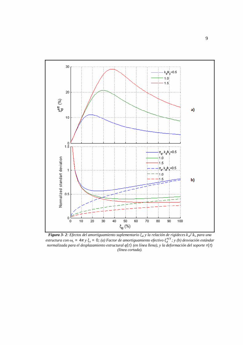
Nótese que al introducir la rigidez del SDS, el modelo tiene amortiguamiento no-
clásico, con una pareja de auto-valores complejos conjugados y un auto-valor real. La
Figura 3- 2.a muestra el factor de amortiguamiento asociado al primer auto-valor de
la matriz de estado (en adelante denominado factor de amortiguamiento efectivo
), en función del factor de amortiguamiento suplementario , para una
estructura con = 4 y = 0, y para = 0.5, 1.0 1.5. Pueden distinguirse dos
regiones: en la primera región, y son aproximadamente iguales, mientras
que en la segunda región es significativamente menor a , llegando incluso a
disminuir después de alcanzar un máximo global. Este valor máximo es mayor a
medida que la rigidez aumenta.
Por otra parte la Figura 3- 2.b muestra en línea llena la desviación estándar del
desplazamiento estructural ( ) calculado para una excitación de tipo ruido blanco, y
normalizado respecto a la desviación estándar para = 0.05 y / = 1.5. Se
puede observar una importante disminución de la respuesta estructural en la primera
región, mientras que en la segunda región la respuesta se mantiene prácticamente
8
constante, llegando incluso a aumentar para el caso en que el SDS es relativamente
flexible ( / = 0.5). En la misma figura, y con línea segmentada, se ha
representado también la desviación estándar normalizada de la deformación del
soporte del SDS ( ). Se puede apreciar que a medida que aumenta, ( ) tiende a
igualarse con ( ), lo que implica que el SDS se comporta realmente como un
“rigidizador”.
Figura 3- 1: Modelo esquemático de un sistema 1 GDL con amortiguamiento suplementario.
9
Figura 3- 2: Efectos del amortiguamiento suplementario y la relación de rigideces / para una estructura con = 4 y = 0; (a) Factor de amortiguamiento efectivo ; y (b) desviación estándar normalizada para el desplazamiento estructural ( ) (en línea llena), y la deformación del soporte ( )
(línea cortada).
10
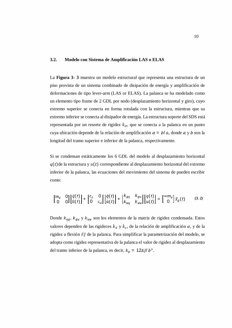
3.2. Modelo con Sistema de Amplificación LAS o ELAS
La Figura 3- 3 muestra un modelo estructural que representa una estructura de un
piso provista de un sistema combinado de disipación de energía y amplificación de
deformaciones de tipo lever-arm (LAS or ELAS). La palanca se ha modelado como
un elemento tipo frame de 2 GDL por nodo (desplazamiento horizontal y giro), cuyo
extremo superior se conecta en forma rotulada con la estructura, mientras que su
extremo inferior se conecta al disipador de energía. La estructura soporte del SDS está
representada por un resorte de rigidez , que se conecta a la palanca en un punto
cuya ubicación depende de la relación de amplificación = / , donde y son la
longitud del tramo superior e inferior de la palanca, respectivamente.
Si se condensan estáticamente los 6 GDL del modelo al desplazamiento horizontal
( )de la estructura y ( ) correspondiente al desplazamiento horizontal del extremo
inferior de la palanca, las ecuaciones del movimiento del sistema de pueden escribir
como:
00 0
( )( ) + 0
0( )( ) + ( )
( ) = 0 ( ) (3. 2)
Donde , y son los elementos de la matriz de rigidez condensada. Estos
valores dependen de las rigideces y , de la relación de amplificación , y de la
rigidez a flexión de la palanca. Para simplificar la parametrización del modelo, se
adopta como rigidez representativa de la palanca el valor de rigidez al desplazamiento
del tramo inferior de la palanca, es decir, = 12 / .
11
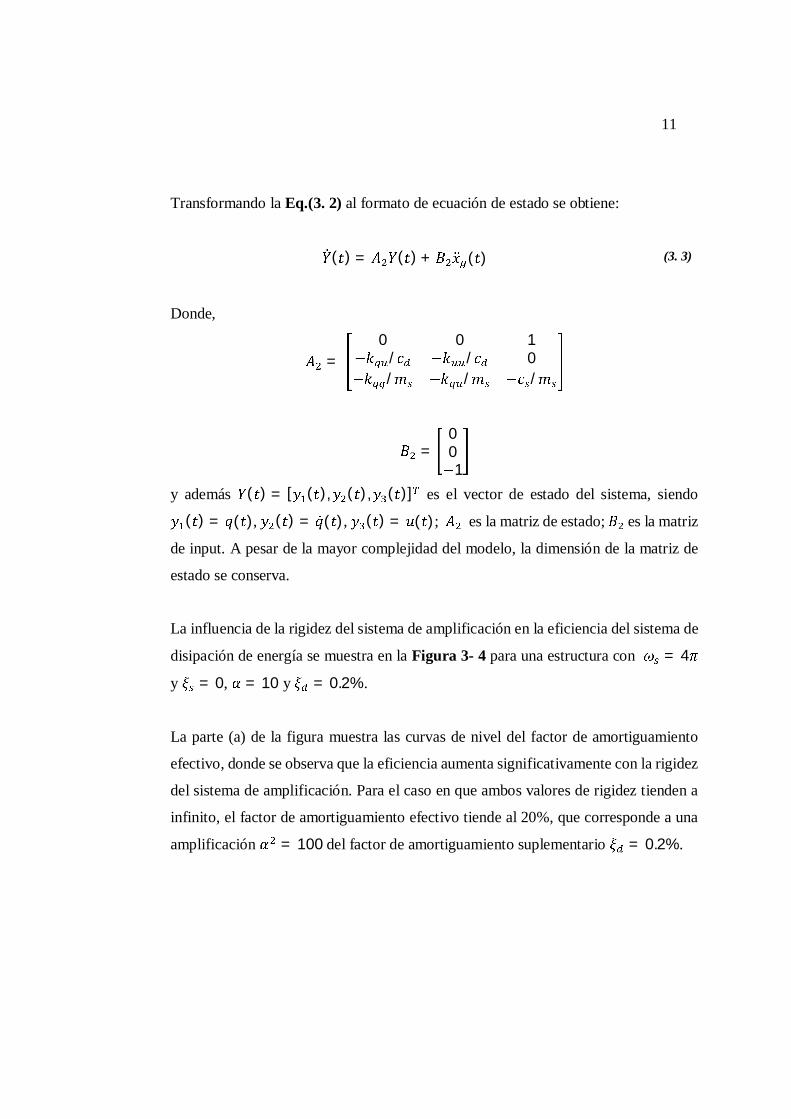
Transformando la Eq.(3. 2) al formato de ecuación de estado se obtiene:
( ) = ( ) + ( ) (3. 3)
Donde,
= 0 0 1
/ / 0/ / /
=001
y además ( ) = [ ( ), ( ), ( )] es el vector de estado del sistema, siendo
( ) = ( ), ( ) = ( ), ( ) = ( ); es la matriz de estado; es la matriz
de input. A pesar de la mayor complejidad del modelo, la dimensión de la matriz de
estado se conserva.
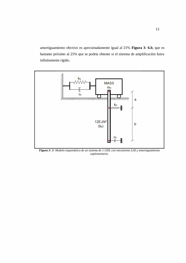
La influencia de la rigidez del sistema de amplificación en la eficiencia del sistema de
disipación de energía se muestra en la Figura 3- 4 para una estructura con = 4
y = 0, = 10 y = 0.2%.
La parte (a) de la figura muestra las curvas de nivel del factor de amortiguamiento
efectivo, donde se observa que la eficiencia aumenta significativamente con la rigidez
del sistema de amplificación. Para el caso en que ambos valores de rigidez tienden a
infinito, el factor de amortiguamiento efectivo tiende al 20%, que corresponde a una
amplificación = 100 del factor de amortiguamiento suplementario = 0.2%.
12
La parte (b) de la figura muestra las curvas de nivel del denominado factor de
amplificación efectivo , definido como el cociente entre los valores absolutos de
los desplazamientos del extremo inferior de la palanca y de la estructura, ambos
asociados al primer auto-vector de la matriz de estado . Las curvas de nivel tienen
una forma similar a la anterior, mostrando que la amplificación efectiva tiende a
la amplificación mecánica a medida que y aumentan. Notar que para alcanzar
una eficiencia mayor al 85% se requiere que la relación / sea mayor o igual que
1, y que la relación / sea mayor o igual a 0.1. Esta figura indica que una relación
/ = 0.1 es adecuada para el diseño.
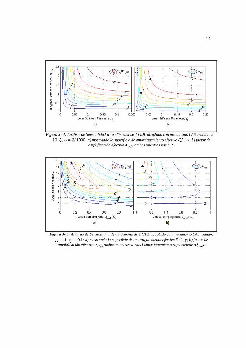
Complementariamente a la Figura 3- 4, se muestra en la Figura 3- 5.a la variación
del factor de amortiguamiento efectivo como función del factor de
amortiguamiento suplementario y de la amplificación mecánica , para una
estructura con = 4 , = 0, / = 1 y / = 0.1. Es interesante notar que
los mayores valores de amortiguamiento efectivo se obtienen para valores altos de
y valores pequeños de . Este resultado se puede entender mejor si se analizan las
curvas de nivel de la amplificación efectiva mostradas la Figura 3- 5.b. Como
era de esperar, se observa que la eficiencia de la palanca disminuye a medida que
aumenta el factor de amortiguamiento suplementario .
La Figura 3- 6 muestra los mismos resultados anteriores, pero usando el formato de
la Figura 3- 2 (correspondiente a la estructura sin sistema de amplificación). Se puede
observar que los mejores resultados se obtienen con sistemas de amplificación rígidos,
amplificación mecánica alta, y factores de amortiguamiento suplementario bajos. Por
ejemplo, si se adopta = 10, / = 1.5, / _ = 0.15 y = 0.25%., se
obtiene una reducción de un 50% de la respuesta. En este caso particular el
13
amortiguamiento efectivo es aproximadamente igual al 21% Figura 3- 6.b, que es
bastante próximo al 25% que se podría obtener si el sistema de amplificación fuera
infinitamente rígido.
Figura 3- 3: Modelo esquemático de un sistema de 1 GDL con mecanismo LAS y amortiguamiento
suplementario.
14
Figura 3- 4: Análisis de Sensibilidad de un Sistema de 1 GDL acoplado con mecanismo LAS usando: =
10; = 2/1000; a) mostrando la superficie de amortiguamiento efectivo , y; b) factor de amplificación efectiva , ambos mientras varia .
Figura 3- 5: Análisis de Sensibilidad de un Sistema de 1 GDL acoplado con mecanismo LAS usando: = 1, = 0.1; a) mostrando la superficie de amortiguamiento efectivo , y; b) factor de
amplificación efectiva , ambos mientras varia el amortiguamiento suplementario .
15
Figura 3- 6: Efectos del amortiguamiento suplementario y la relación de rigideces / para una estructura con = 4 y = 0, razón de amortiguamiento efectivo y desviación estándar
normalizada del desplazamiento estructural ( ) para; a) = 5 y, b) = 10.
16
4. MODELO DE MÚLTIPLES GRADOS DE LIBERTAD
4.1. Modelo de Edificio de 7 Pisos
Una vez evaluado el sistema de un grado de libertad en las secciones precedentes, en
la presente sección se analiza el comportamiento del mecanismo de amplificación
propuesto instalado en un sistema de múltiples grados de libertad.
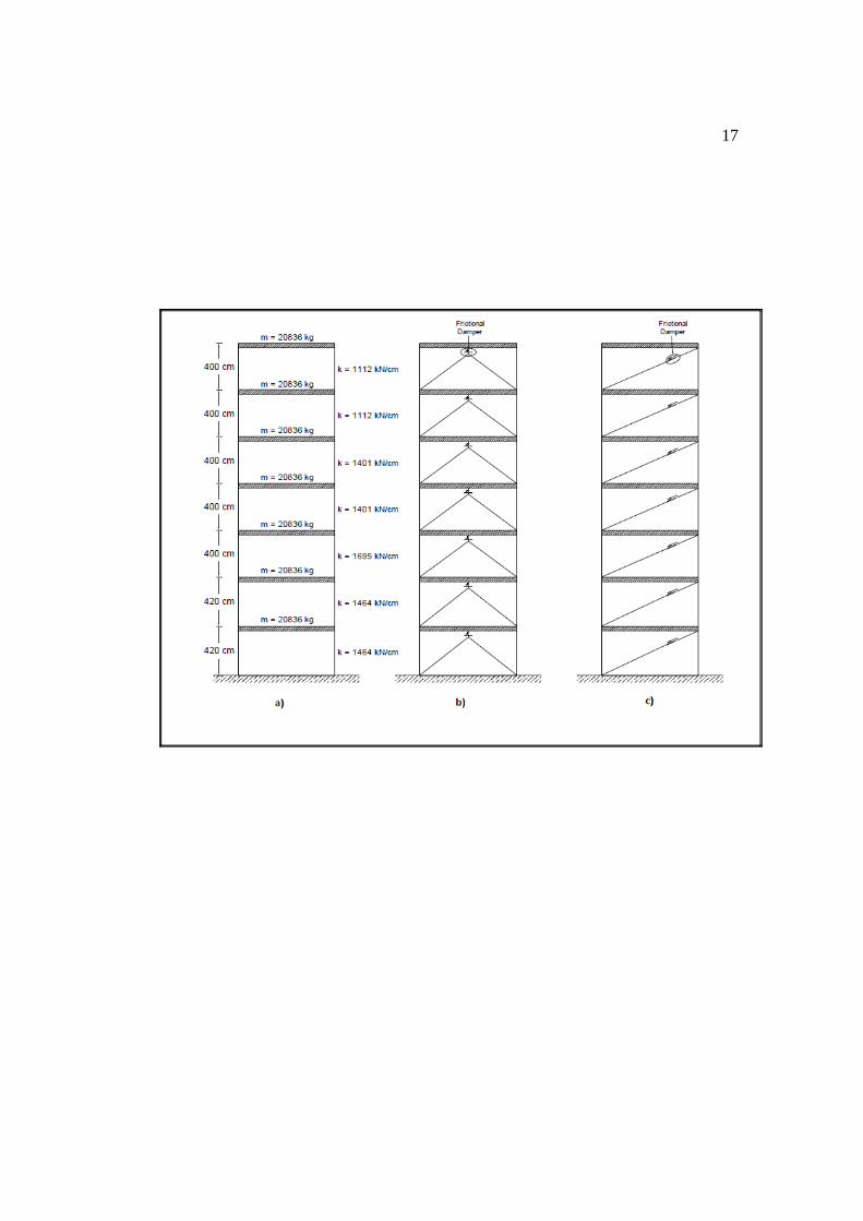
En la Figura 4- 1.a, se muestra el modelo de un edificio de 7 pisos sin ningún
mecanismo de protección sísmica instalado en él. Las propiedades de masa y rigidez
de cada piso se indican en la figura.
Es importante recalcar que se ha considerado que los pisos se desplazan
horizontalmente sin deformación axial de vigas ni columnas, asumiendo un
comportamiento a manera de diafragma rígido en piso. Debido a esta supuesto, se
tiene 7 grados de libertad de desplazamiento horizontal y el periodo fundamental del
edificio es de = 0.50 segundos.
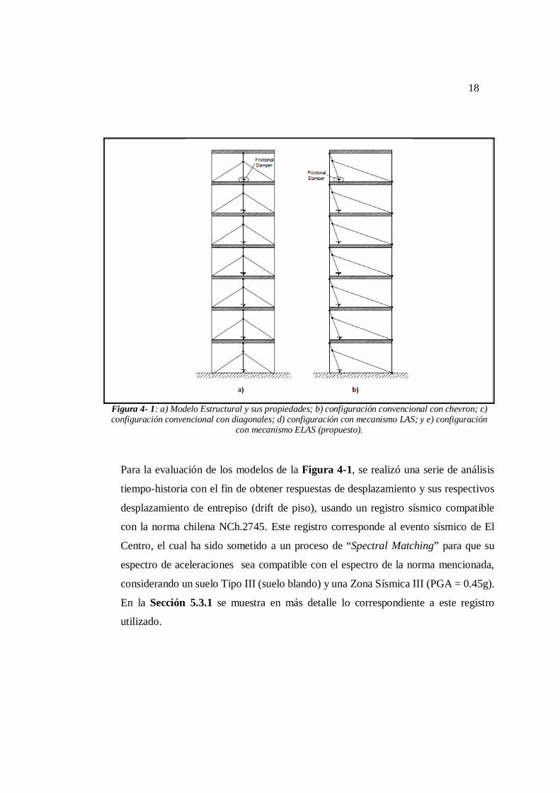
Nótese que en la Figura 4- 1.b, se modela la estructura con el método convencional
tipo chevron para la instalación de disipadores de energía, mientras que en la Figura
4- 1.c, la segunda configuración convencional basada en diagonales. Las Figura 4-
1.d y Figura 4- 1.e muestran las configuraciones con LAS y ELAS respectivamente,
siendo esta ultima la propuesta en esta investigación.
17
18
Figura 4- 1: a) Modelo Estructural y sus propiedades; b) configuración convencional con chevron; c) configuración convencional con diagonales; d) configuración con mecanismo LAS; y e) configuración
con mecanismo ELAS (propuesto).
Para la evaluación de los modelos de la Figura 4-1, se realizó una serie de análisis
tiempo-historia con el fin de obtener respuestas de desplazamiento y sus respectivos
desplazamiento de entrepiso (drift de piso), usando un registro sísmico compatible
con la norma chilena NCh.2745. Este registro corresponde al evento sísmico de El
Centro, el cual ha sido sometido a un proceso de “Spectral Matching” para que su
espectro de aceleraciones sea compatible con el espectro de la norma mencionada,
considerando un suelo Tipo III (suelo blando) y una Zona Sísmica III (PGA = 0.45g).
En la Sección 5.3.1 se muestra en más detalle lo correspondiente a este registro
utilizado.
19
Para la distribución en altura de dispositivos de disipación de energía, se ha usado el
algoritmo SSSA (Simplified Sequential Search Algorithm) (Lopez-García, 2001) y
(Lopez-Garcia & Soong, 2002) considerando que la capacidad de las unidades de
disipación para las instalaciones convencionales (1 y 2) será diferente en relación a
las unidades que se usarán en las configuraciones con amplificadores (3 y 4). Para las
configuraciones convencionales por ejemplo, la capacidad de los disipadores se
establecen en = 5000 , mientras que para las configuraciones con mecanismo
de amplificación se define un = 500 . Nótese que la relación / es igual
a 10, que es el mismo valor que se da al factor de amplificación para estos análisis, es
decir = 10. Es importante mencionar que, para la distribución por medio del SSSA,
se ha establecido un drift de piso objetivo de = 2.5/1000.
Por otra parte, para asegurar que la comparación de los resultados en esta etapa sean
lo más acertados posible, se dimensionan los elementos constitutivos en las
configuraciones 1 al 4 (diagonales, chevrones, palancas y tensores) tomando en cuenta
que sus rigideces sean las necesarias como para trabajar elásticamente (sección
transversal de 0.018 ) y con deformaciones pequeñas bajo el efecto de un disipador
cuya fuerza de activación llegue a ser de 60.000 kgf (lo cual no sucede en este análisis)
y así garantizar que las 4 configuraciones trabajen con la máxima eficiencia posible.
El análisis dinámico tiempo-historia se realizó por medio de simulación por
computadora. Se generó rutinas para los programas OpenSees (McKenna, Fenves,
Scott, & Jeremic, 2000) y MATLAB (“MATLAB,” 2013) que trabajaran en conjunto
para obtener los resultados requeridos. El primero de ellos fue usado para generar los
modelos completos de las estructuras, por medio de MATLAB, se ejecutaba el
programa OpenSees, de este se obtenía la respuesta de desplazamientos de piso. Con
estos desplazamientos se calcula, usando MATLAB, los drift de piso y en base a esta
20
respuesta se ejecuta de manera secuencial los análisis consecutivos nuevamente en
OpenSees.
Tabla 4- 1: Número de Unidades necesarias
Piso Diagonales Chevrones LAS ELAS 1 24 21 18 18 2 15 14 12 14 3 4 4 1 0 4 3 3 2 0 5 0 0 0 0 6 0 0 0 0 7 0 0 0 0
TOTAL 46 42 33 32
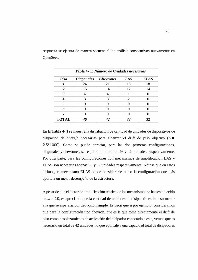
En la Tabla 4- 1 se muestra la distribución de cantidad de unidades de dispositivos de
disipación de energía necesarias para alcanzar el drift de piso objetivo ( =
2.5/1000). Como se puede apreciar, para las dos primeras configuraciones,
diagonales y chevrones, se requieren un total de 46 y 42 unidades, respectivamente.
Por otra parte, para las configuraciones con mecanismos de amplificación LAS y
ELAS son necesarias apenas 33 y 32 unidades respectivamente. Nótese que en estos
últimos, el mecanismo ELAS puede considerarse como la configuración que más
aporta a un mejor desempeño de la estructura.
A pesar de que el factor de amplificación teórico de los mecanismos se han establecido
en = 10, es apreciable que la cantidad de unidades de disipación es incluso menor
a la que se esperaría por deducción simple. Es decir que si por ejemplo, consideramos
que para la configuración tipo chevron, que es la que toma directamente el drift de
piso como desplazamiento de activación del disipador conectado a este, vemos que es
necesario un total de 42 unidades, lo que equivale a una capacidad total de disipadores
21
de = 42 500 = 210000 . Si contrastamos esta capacidad total
con la obtenida del mecanismo ELAS que es = 16000 de las 32
unidades necesarias en total, podemos observar que la razón entre estos dos valores
es = / = 13.1, mayor al factor de amplificación teórico.
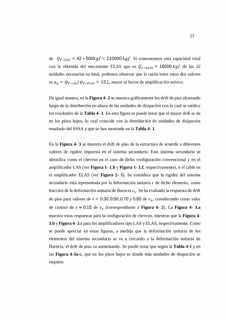
De igual manera, en la Figura 4- 2 se muestra gráficamente los drift de piso alcanzado
luego de la distribución en altura de las unidades de disipación con lo cual se ratifica
los resultados de la Tabla 4- 1. En esta figura se puede notar que el mayor drift se da
en los pisos bajos, lo cual coincide con la distribución de unidades de disipación
resultado del SSSA y que se han mostrado en la Tabla 4- 1.
En la Figura 4- 3 se muestra el drift de piso de la estructura de acuerdo a diferentes
valores de rigidez impuesta en el sistema secundario. Este sistema secundario se
identifica como el chevron en el caso de dicha configuración convencional y en el
amplificador LAS (ver Figura 1- 1.b y Figura 1- 1.f, respectivamente), o el cable en
el amplificador ELAS (ver Figura 2- 1). Se considera que la rigidez del sistema
secundario está representada por la deformación unitaria de dicho elemento, como
fracción de la deformación unitaria de fluencia . Se ha evaluado la respuesta de drift
de piso para valores de = 0.30, 0.50, 0.70 0.95 de , considerando como valor
de control de 0.15 de (correspondiente a Figura 4- 2). La Figura 4- 3.a
muestra estas respuestas para la configuración de chevron, mientras que la Figura 4-
3.b y Figura 4- 3.c para los amplificadores tipo LAS y ELAS, respectivamente. Como
se puede apreciar en estas figuras, a medida que la deformación unitaria de los
elementos del sistema secundario se va a cercando a la deformación unitaria de
fluencia, el drift de piso va aumentando. Se puede notar que según la Tabla 4-1 y en
las Figura 4-3a-c. que en los pisos bajos es donde más unidades de disipación se
requiere.
22
l Figura 4- 2: Drift de piso después de hacer la distribución en altura de los dispositivos de disipación
usando el método SSSA.
1
2
3
4
5
6
7
1 2 3 4 5 6
Stor
y
Story Drift [‰]
No Dissipation
Diagonal Config.
Target
Chevron Config.
LAS Amplifier
ELAS Amplifier
23
a
Figura 4- 3: Deriva de piso calculada a medida que varía para: (a) configuración con chevrones; (b) mecanismo LAS; (c) mecanismo ELAS; y (d) eficiencia de la configuración, mientras varia.
Se presenta en la Figura 4- 3.d, a manera de resumen de los resultados presentados
de drift de piso mencionados en los párrafos anteriores, la eficiencia de los tres
dispositivos de este análisis en función de la relación = / . Esta eficiencia se
calcula relacionando los valores de drift de piso para la condición óptima, es decir,
luego de la distribución usando el algoritmo SSSA con los miembros del sistema
secundario rígidos, con cada relación para los drift del primer piso. Nótese que la
1
2
3
4
5
6
7
1 2 3 4 5 6
Stor
y
Story Drift [‰]
No Dissipation
Target
< 20 % of y
30% of y
50% of y
70% of y
95% of y
1
2
3
4
5
6
7
1 2 3 4 5 6
Stor
y
Story Drift [‰]
NoDissipationTarget
< 20 % of y
30% of y
50% of y
1
2
3
4
5
6
7
1 2 3 4 5 6
Stor
y
Story Drift [‰]
No Dissipation
Target
< 20 % of y
30% of y
50% of y
70% of y
95% of y
0%
10%
20%
30%
40%
50%
60%
70%
80%
90%
100%
0.3 0.4 0.5 0.6 0.7 0.8 0.9
EFFI
CIEN
CY-
= / y
Chevron Config.
LAS Amplifier
ELAS Amplifier
(b)
(c)
(a)
(d)
24
eficiencia de ambos dispositivos, LAS y ELAS son muy similares debido a su similar
funcionamiento y que la diferencia a favor de este último dispositivo respalda los
resultados de la Tabla 4- 1 de cantidades de unidades necesarias para alcanzar un
determinado drift objetivo.
Esta pequeña diferencia puede darse por la ubicación de donde entrega la fuerza de
amortiguamiento amplificada el amplificador LAS. Este, a diferencia del amplificador
propuesto ELAS, entrega dicha fuerza a una zona poco rígida del pórtico y la
transmisión final a los demás elementos de soporte puede verse afectada por la
flexibilidad de la viga a donde está conectada. A diferencia del amplificador ELAS
que entrega la fuerza de amortiguamiento a una zona rígida del pórtico que es el nudo
de unión viga-columna, haciendo más eficiente el efecto de esta fuerza en la
estructura.
4.2. Modelo de Edificio de 5 pisos. Sistema Dual (Muro-Pórtico)
Como es bien sabido, los muros de hormigón armado son muy eficientes para
controlar las deformaciones de entrepiso en estructuras sometidas a excitación
sísmica. Sin embargo, esta característica dificulta el uso de sistemas de disipación de
energía. La Figura 4- 4 muestra un modelo estructural plano de 5 pisos de hormigón
armado, conformado por un marco de 2 vanos y un muro, donde se ha incorporado un
sistema de amplificación tipo ELAS. Para mostrar la influencia de la rigidez de las
diagonales se han considerado dos casos, en los que la relación entre la sección de las
diagonales es igual a 2. Las dimensiones de los elementos estructurales principales y
secundarios, como también el peso sísmico de cada piso se indican en la Tabla 4- 2 .
El periodo fundamental de la estructura es igual To=0.39 s. La Figura 4- 5 presenta
las historias de energía (histerética) disipada por los dispositivos friccionales, y la
energía (viscosa) disipada por la estructura principal. Se puede observar que a mayor
25
rigidez de las diagonales, mayor es la energía histerética y menor la energía viscosa
disipada.
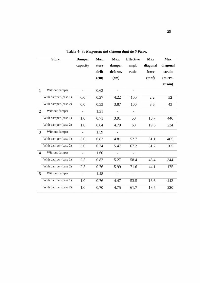
La Tabla 4- 3 presenta un resumen de los resultados obtenidos para la estructura con
y sin disipadores de energía. A pesar de que todos los indicadores de desempeño de
la estructura con diagonales rígidas son mejores a los de su contraparte flexible, esta
última entrega resultados que podríamos considerar satisfactorios. Nótese además que
con una capacidad total de sólo 7.5 tonf, se consigue reducir las deformaciones de
entrepiso máximas en aproximadamente un 50%, a pesar de que la eficiencia
promedio del sistema de amplificación es de 65% y 70% para los casos con diagonales
flexibles y rígidas, respectivamente. Para ilustrar este importante aspecto, la Figura
4- 6 muestra las historias de deformación de los disipadores de energía, y de las
deformaciones de entrepiso multiplicadas por el factor de amplificación teórico ( =
11). Notar que la eficiencia alcanza el 100% sólo en el primer piso, donde no se
necesitan disipadores de energía.

26
Figura 4- 4: Modelo estructural del sistema dual analizado.

27
Tabla 4- 2: Propiedades Estructurales. Modelo de Sistema dual de 5 pisos.
Story Heigth
(cm)
Seismic
weigth
(tonf)
Principal structure’s
elements
Secondary structure’s
elements
Column
section
(cm)
Beam
section
(cm)
Wall
section
(cm)
Lever
arm
inertia
(cm4)
Diagonal area
(cm2)
Case 1 Case 2
1 325 40 60 x 60 30 x 50 15 x 300 7786 20 40
2 325 40 60 x 60 30 x 50 15 x 300 7786 20 40
3 325 40 60 x 60 30 x 50 15 x 300 7786 60 120
4 325 40 60 x 60 30 x 50 15 x 300 7786 60 120
5 325 20 60 x 60 30 x 50 15 x 300 7786 20 40
Figura 4- 5: Historia de energía disipada en el sistema.
28
Figura 4- 6: Historia de respuesta de deformación de cada piso y de los dispositivos de disipación ( veces).
29
Tabla 4- 3: Respuesta del sistema dual de 5 Pisos.
Story Damper
capacity
Max.
story
drift
(cm)
Max.
damper
deform.
(cm)
Effective
ampl.
ratio
Max
diagonal
force
(tonf)
Max
diagonal
strain
(micro-
strain)
1 Without damper - 0.63 - - With damper (case 1) 0.0 0.37 4.22 100 2.2 52 With damper (case 2) 0.0 0.33 3.87 100 3.6 43
2 Without damper - 1.31 - - With damper (case 1) 1.0 0.71 3.91 50 18.7 446 With damper (case 2) 1.0 0.64 4.79 68 19.6 234
3 Without damper - 1.59 - With damper (case 1) 3.0 0.83 4.81 52.7 51.1 405 With damper (case 2) 3.0 0.74 5.47 67.2 51.7 205
4 Without damper - 1.60 - - With damper (case 1) 2.5 0.82 5.27 58.4 43.4 344 With damper (case 2) 2.5 0.76 5.99 71.6 44.1 175
5 Without damper - 1.48 - - With damper (case 1) 1.0 0.76 4.47 53.5 18.6 443 With damper (case 2) 1.0 0.70 4.75 61.7 18.5 220
30
5. ESTUDIO EXPERIMENTAL
Con el fin de evaluar el comportamiento real del mecanismo de amplificación de
desplazamientos (ELAS) propuesto en esta investigación, se realizaron una serie de
ensayos pseudo-dinámicos en el Laboratorio del Departamento de Ingeniería Estructural
y Geotécnica. Éstos fueron ejecutados sobre una estructura metálica a escala real cuyas
características se detallan en la siguiente sección, construida especialmente para dar
sustento experimental a una serie de investigaciones realizadas a la par de la presente.
Una de estas es la que se presenta en (Tapia Flores, 2015).
En este capítulo, se da una breve descripción de la estructura de prueba y cómo se instaló
el mecanismo de amplificación en uno de los pórticos de ésta, así como también la
implementación de un tipo convencional de dispositivo de disipación de energía en este
conjunto amplificador-estructura.
Una descripción más detallada de la evaluación realizada la estructura metálica para
determinar sus propiedades mecánicas, se puede obtener de (Tapia Flores, 2015). En esta
investigación se describen ensayos adicionales realizados a la estructura de prueba, de
donde se ha podido estimar parámetros, como por ejemplo, el amortiguamiento intrínseco
considerable que posee el espécimen debido al tipo de conexiones apernadas con el que
fue concebido, entre otras consideraciones.
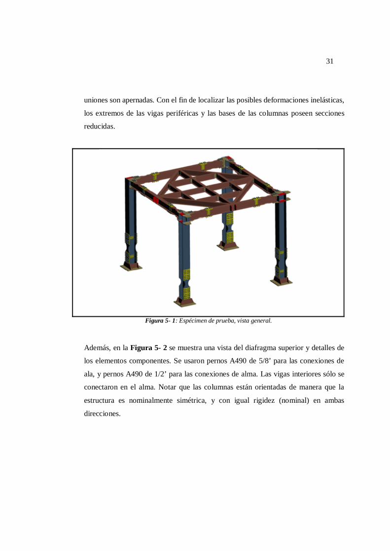
5.1. Espécimen de Prueba e instalación del mecanismo ELAS
La Figura 5- 1 muestra una vista esquemática del espécimen de prueba. Las 4
columnas tienen una sección HN30×106, mientras que las vigas perimetrales e
interiores tienen una sección IN25×32.6 y IN20×19.8, respectivamente. Con el
propósito de generar una estructura reconfigurable y de fácil montaje, todas las
31
uniones son apernadas. Con el fin de localizar las posibles deformaciones inelásticas,
los extremos de las vigas periféricas y las bases de las columnas poseen secciones
reducidas.
Figura 5- 1: Espécimen de prueba, vista general.
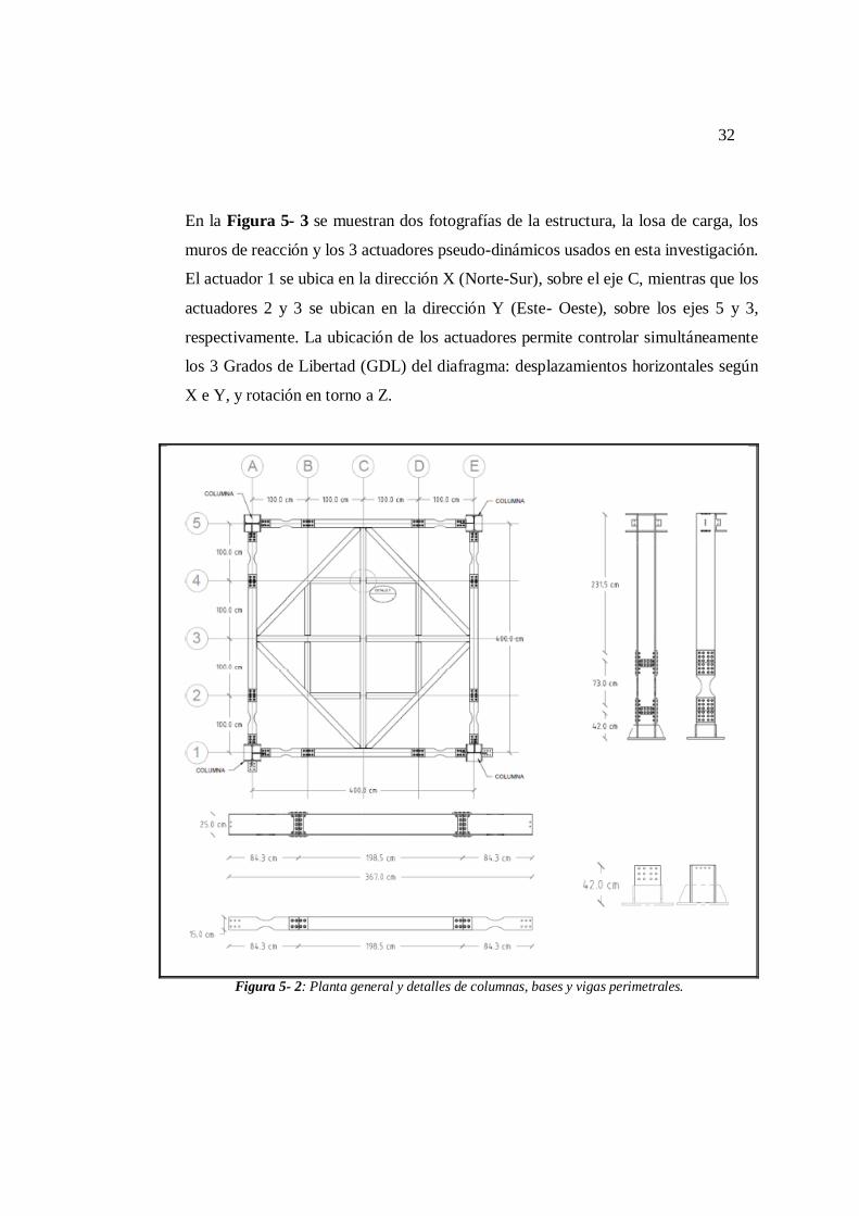
Además, en la Figura 5- 2 se muestra una vista del diafragma superior y detalles de
los elementos componentes. Se usaron pernos A490 de 5/8’ para las conexiones de
ala, y pernos A490 de 1/2’ para las conexiones de alma. Las vigas interiores sólo se
conectaron en el alma. Notar que las columnas están orientadas de manera que la
estructura es nominalmente simétrica, y con igual rigidez (nominal) en ambas
direcciones.
32
En la Figura 5- 3 se muestran dos fotografías de la estructura, la losa de carga, los
muros de reacción y los 3 actuadores pseudo-dinámicos usados en esta investigación.
El actuador 1 se ubica en la dirección X (Norte-Sur), sobre el eje C, mientras que los
actuadores 2 y 3 se ubican en la dirección Y (Este- Oeste), sobre los ejes 5 y 3,
respectivamente. La ubicación de los actuadores permite controlar simultáneamente
los 3 Grados de Libertad (GDL) del diafragma: desplazamientos horizontales según
X e Y, y rotación en torno a Z.
Figura 5- 2: Planta general y detalles de columnas, bases y vigas perimetrales.

33
Figura 5- 3: Espécimen de prueba sobre losa de reacción y acoplado al equipo pseudo-dinámico.
La Figura 5- 4 muestra un esquema del sistema de amplificación que se propone en
esta investigación, como también una fotografía del eje A con el disipador tipo
friccional lineal instalado entre la barra colectora del amplificador y la losa de carga.
El sistema de amplificación tiene una relación de amplificación teórica = 11.
Figura 5- 4: Esquema del mecanismo de Amplificación e instalación en el pórtico exterior del espécimen de prueba.
34
5.2. Amortiguador Friccional
Es importante recalcar que hasta la actualidad, es muy común encontrar publicaciones
de investigación de mecanismos de amplificación de desplazamientos, validados por
ensayos experimentales acompañados de dispositivos de disipación de energía tipo
viscoso lineal y no lineal.
En publicaciones como (Mualla & Belev, 2002) y en (Kim, Choi, & K.-W., 2011) sin
embargo, se expone la utilización de un disipador tipo friccional, que si bien es cierto
no está acoplado a un mecanismo de amplificación, está instalado por medio de
tensores a la estructura. La instalación de estos dispositivos, tal como se muestra en
las mencionadas publicaciones, se ubica de tal forma que la fuerza de disipación es
aplicada directamente a la mitad de la luz de cada viga en el pórtico donde se instala.
Es nuestra intención hacer notar que con el mecanismo ELAS propuesto en esta
investigación, cualquier tipo de dispositivo de disipación de energía puede ser
instalado en una estructura, manteniendo siempre la configuración y uno de los
preceptos fundamentales consistente en entregar idealmente la fuerza de disipación a
una zona rígida de la estructura (unión viga-columna).
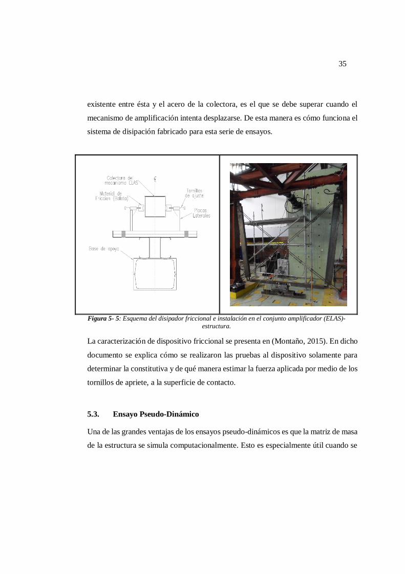
La Figura 5- 5 muestra un esquema del dispositivo de disipación de energía y una
fotografía de la instalación de éste en el espécimen de prueba, acoplado al mecanismo
de amplificación de desplazamientos. Este dispositivo friccional se asemeja a un
medio camisón en forma de C, de dimensiones mayores a las de la barra colectora del
mecanismo ELAS. El disipador actúa cuando los tornillos que se indican en la Figura
5- 5 son ajustados, haciendo que las placas laterales se deformen aplicando a su vez
una presión a la barra colectora. Esta presión es aplicada a la colectora por medio de
dados de acero en los extremos de los tornillos, donde está instalada una semiesfera
de balata. La presión transmitida por la balata junto con el coeficiente de rozamiento
35
existente entre ésta y el acero de la colectora, es el que se debe superar cuando el
mecanismo de amplificación intenta desplazarse. De esta manera es cómo funciona el
sistema de disipación fabricado para esta serie de ensayos.
Figura 5- 5: Esquema del disipador friccional e instalación en el conjunto amplificador (ELAS)-estructura.
La caracterización de dispositivo friccional se presenta en (Montaño, 2015). En dicho
documento se explica cómo se realizaron las pruebas al dispositivo solamente para
determinar la constitutiva y de qué manera estimar la fuerza aplicada por medio de los
tornillos de apriete, a la superficie de contacto.
5.3. Ensayo Pseudo-Dinámico
Una de las grandes ventajas de los ensayos pseudo-dinámicos es que la matriz de masa
de la estructura se simula computacionalmente. Esto es especialmente útil cuando se
36
tratan de simular efectos torsionales, ya que podemos arbitrariamente cambiar no
solamente la cantidad de masa, sino también su distribución en planta.
Como es bien sabido (Mahin & Shing, 1985), (Aktan & Asce, 1986) y (Nakashima,
Kato, & Takaoka, 1992), un ensayo pseudo-dinámico consiste en resolver paso a paso
la siguiente ecuación diferencial matricial:
( ) + ( ) + ( ) = ( ) (5. 1)
Donde es la matriz de masa; es la matriz de amortiguamiento clásico; ( ) es e
vector de grados de libertad (GDL) de la estructura; ( ) es el vector de fuerzas
restitutivas (elásticas y/o inelásticas); y es el vector de aceleraciones del suelo,
siendo la matriz de incidencia sobre los GDL de la estructura.
En un ensayo pseudo dinámico, se establece como datos de entrada la matriz de
amortiguamiento clásico y la matriz de masa de la estructura. La ventaja de este tipo
de ensayo es que se puede establecer diferentes propiedades dinámicas a la estructura
de prueba solamente variando la matriz de masa que es introducida por el usuario y la
matriz de rigidez es determinada paso a paso en función de las mediciones tomadas
por las celdas de carga en los actuadores y los desplazamientos impuestos obtenidos
también en cada paso de integración. La ecuación del movimiento es resuelta por
integración paso a paso, en este caso usando el integrador Newmark explicito
incorporado al Módulo de ensayo Pseudo-Dinámico provisto por la empresa ARIES.
La matriz de masa, como se ha mencionado en el párrafo anterior, es calculada según
la necesidad de las condiciones de ensayo. Esta es determinada en función del radio
37
de giro de la masa , la masa y la excentricidad de la ubicación con respecto al
centro geométrico de la planta.
= 0
0 00
(5. 2)
Donde, para nuestra evaluación experimental tenemos = 31060 como masa
traslacional; = 1.0 como excentricidad de masa; y = 2.35 como radio de
giro.
En (Tapia Flores, 2015) se demuestra por medio de ensayos de vibraciones libres, que
la estructura como tal, por su tipo de conexiones apernadas (deslizamiento entre placas
de conexión y elementos) posee un amortiguamiento intrínseco alto. Es por esto que
se introduce una matriz nula como dato.
La Figura 5- 6 muestra una implantación del espécimen de prueba ubicado sobre la
losa de reacción y conectada a los actuadores pseudo-dinámicos apoyados al muro de
reacción.
38
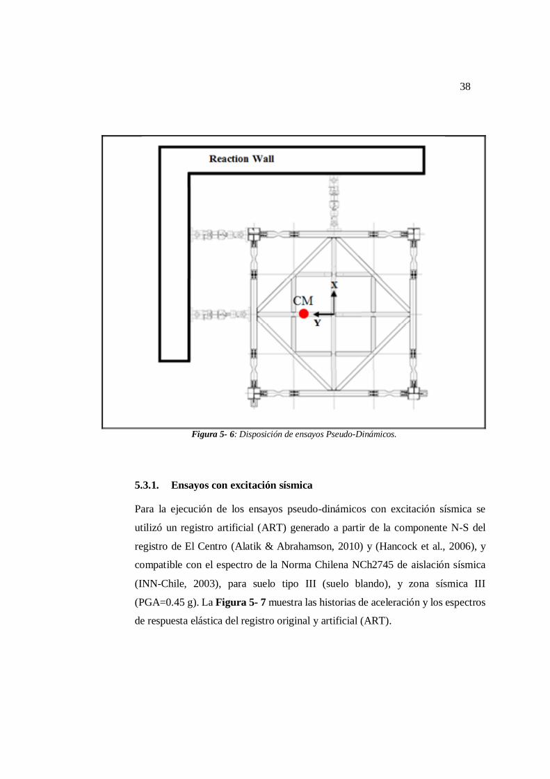
Figura 5- 6: Disposición de ensayos Pseudo-Dinámicos.
5.3.1. Ensayos con excitación sísmica
Para la ejecución de los ensayos pseudo-dinámicos con excitación sísmica se
utilizó un registro artificial (ART) generado a partir de la componente N-S del
registro de El Centro (Alatik & Abrahamson, 2010) y (Hancock et al., 2006), y
compatible con el espectro de la Norma Chilena NCh2745 de aislación sísmica
(INN-Chile, 2003), para suelo tipo III (suelo blando), y zona sísmica III
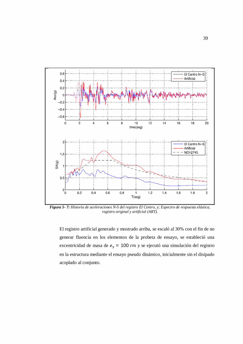
(PGA=0.45 g). La Figura 5- 7 muestra las historias de aceleración y los espectros
de respuesta elástica del registro original y artificial (ART).
39
Figura 5- 7: Historia de aceleraciones N-S del registro El Centro, y; Espectro de respuesta elástica,
registro original y artificial (ART).
El registro artificial generado y mostrado arriba, se escaló al 30% con el fin de no
generar fluencia en los elementos de la probeta de ensayo, se estableció una
excentricidad de masa de = 100 y se ejecutó una simulación del registro
en la estructura mediante el ensayo pseudo dinámico, inicialmente sin el disipado
acoplado al conjunto.
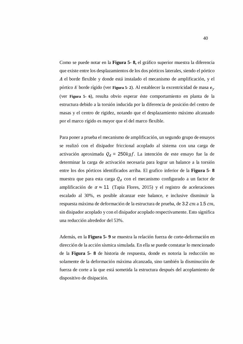
40
Como se puede notar en la Figura 5- 8, el gráfico superior muestra la diferencia
que existe entre los desplazamientos de los dos pórticos laterales, siendo el pórtico
el borde flexible y donde está instalado el mecanismo de amplificación, y el
pórtico borde rígido (ver Figura 5- 2). Al establecer la excentricidad de masa
(ver Figura 5- 6), resulta obvio esperar éste comportamiento en planta de la
estructura debido a la torsión inducida por la diferencia de posición del centro de
masas y el centro de rigidez, notando que el desplazamiento máximo alcanzado
por el marco rígido es mayor que el del marco flexible.
Para poner a prueba el mecanismo de amplificación, un segundo grupo de ensayos
se realizó con el disipador friccional acoplado al sistema con una carga de
activación aproximada = 250 . La intención de este ensayo fue la de
determinar la carga de activación necesaria para lograr un balance a la torsión
entre los dos pórticos identificados arriba. El grafico inferior de la Figura 5- 8
muestra que para esta carga con el mecanismo configurado a un factor de
amplificación de 11 (Tapia Flores, 2015) y el registro de aceleraciones
escalado al 30%, es posible alcanzar este balance, e inclusive disminuir la
respuesta máxima de deformación de la estructura de prueba, de 3.2 a 1.5 ,
sin disipador acoplado y con el disipador acoplado respectivamente. Esto significa
una reducción alrededor del 53%.
Además, en la Figura 5- 9 se muestra la relación fuerza de corte-deformación en
dirección de la acción sísmica simulada. En ella se puede constatar lo mencionado
de la Figura 5- 8 de historia de respuesta, donde es notoria la reducción no
solamente de la deformación máxima alcanzada, sino también la disminución de
fuerza de corte a la que está sometida la estructura después del acoplamiento de
dispositivo de disipación.
41
Figura 5- 8: Comparación desplazamientos en los bordes sin disipador (arriba) y con disipador (abajo).
Registro escalado al 30%, excentricidad e=100 cm.
Adicionalmente, en la misma Figura 5- 9 se muestra la relación rotación-
deformación, en ella puede observar además la disminución de los efectos de
torsión logrados al minimizar la respuesta en el eje flexible de la estructura de
prueba luego de acoplar el dispositivo de disipación friccional.
42
Figura 5- 9: Comparación respuestas sin disipador. Relación fuerza-desplazamiento en el centro
geométrico (izquierda); y relación desplazamiento en el centro geométrico vs rotación de la planta (derecha). Registro escalado al 30%, excentricidad e=100 cm.
Finalmente, en la gráfica superior de la Figura 5- 10, se muestra la deformación
del amortiguador (línea azul continua) y la deformación del eje flexible
multiplicada por el factor de amplificación del mecanismo, = 11. Como se
puede notar en esta gráfica, las deformaciones alcanzadas en el disipador son muy
similares a las que esta inducido el pórtico. Las planicies que se pueden identificar
en la historia de deformaciones correspondiente al disipador, se pueden explicar
debido al comportamiento propio de un disipador friccional, donde, antes de
alcanzar el peak en deformación, el dispositivo se traba y es necesario volver a
romper la fuerza de rozamiento para cambiar de sentido a la deformación.

43
Figura 5- 10: Respuestas con disipador. Deformación real vs “ideal” del disipador (arriba); y
deformaciones unitarias en los tensores (abajo). Registro escalado al 30%, excentricidad e=100 cm.
En la gráfica inferior de la Figura 5- 10 se encuentra identificado la historia de
deformación unitaria de los tensores (T1, T2, T3 y T4) del mecanismo de amplificación
(ver Figura 5- 4). Nótese que la deformación unitaria máxima alcanzada en los tensores es
de aproximadamente 580 micro-strains. Para estos tensores, fabricados con acero dulce
cuyo = 4200 / , la deformación unitaria de fluencia es de 2000 micro-
strains, lo que significa que los tensores trabajaron a un = 0.29.
Si nos fijamos en la Figura 4- 3.d, se muestra que para una relación = 0.30, la
eficiencia esperada es de alrededor del 95%, por lo tanto, los resultados mostrados en
44
la Figura 5- 10 son bastante consistentes con la evaluación analítica de eficiencia del
mecanismo en función de la rigidez relativa de los elementos de soporte (tensores) del
amplificador. Además, del estudio realizado en la Sección 3.2 se corrobora también que
para valores de amortiguamiento adicional ( ) bajos, traducidos en este caso en la
fuerza de activación del dispositivo friccional , es posible también alcanzar eficiencias
altas del mecanismo de amplificación y obtener una disminución de la respuesta
estructural apreciable como se indicó anteriormente en esta misma sección.
Lo dicho en párrafos anteriores nos permite aceptar satisfactoriamente los resultados
obtenidos en este capítulo de evaluación experimental.
45
6. CONCLUSIONES
- Se pone en evidencia que gran parte de los mecanismos destinados a amplificar
deformaciones dentro de un sistema estructural, aprovechan la teoría de
apalancamiento para generar esta ventaja mecánica. El mecanismo aquí propuesto
no es una excepción, sin embargo, su configuración geométrica es novedosa y de
fácil construcción. Su propiedad de trabajar en cualquiera de los dos sentidos de
la dirección horizontal de análisis hace que, pese a su ocupación en el vano, éste
sea eficiente al momento de activarse.
- El mecanismo de amplificación propuesto, ELAS, es una variante al sistema LAS
ya analizado anteriormente (Ribakov & Reinhorn, 2003), sin embargo ha
demostrado poseer grandes bondades con factores de amplificación altos, no
alcanzados por otros mecanismos.
- Gracias a lo mencionado anteriormente, es posible que este mecanismo de
amplificación propuesto, trabaje adecuadamente con disipadores de tipo friccional
(Montaño, 2015) y disipadores histeréticos (Tapia Flores, 2015). Estos disipadores
pueden llegar a tener poca o ninguna limitación en cuanto a su recorrido o
deformación alcanzada durante un evento dinámico y a pesar de esto, la
evaluación de este conjunto disipador friccional/histeretico-amplificador en otras
publicaciones casi no estaba disponible hasta el momento. Los factores de
amplificación entregados por el mecanismo ELAS aquí propuesto entonces, puede
ser mejor aprovechado por estos tipos de disipadores, en contraste con disipadores
viscosos que al requerir un recorrido más largo, pueden encarecer los costos del
sistema en conjunto.
46
- De la evaluación analítica tanto para sistemas de 1 GDL como para sistemas de
MGDL, se pudo llegar a determinar que la implementación del mecanismo de
amplificación junto con disipadores friccionales disminuía en gran parte la
respuesta estructural (medida como derivas de piso). En la Sección 3 se establece
la necesidad de que el sistema de soporte del mecanismo de amplificación, en este
caso los tensores, posean una rigidez relativamente alta, para que junto con un
bajo nivel de amortiguamiento añadido, , se pueda alcanzar una gran
eficiencia en el mecanismo con factores de amplificación altos. Por otra parte, de
la Sección 4 se establece que el mecanismo ELAS, a pesar de ser una variante del
mecanismo LAS, trabaja de mejor manera, requiriendo menos unidades de
disipación en una distribución SSSA (Lopez-García, 2001). Esto en parte porque
la fuerza de amortiguamiento se entrega directamente una la zona rígida del
pórtico (unión viga-columna ) y no a una zona mas flexible que colabora con la
perdida de eficiencia al momento de transmitir este esfuerzo.
- Todo lo mencionado anteriormente acerca de la evaluación analítica ha sido
ratificado en la evaluación experimental, donde fue notorio que para valores de
activación bajos del disipador friccional usado, = 250 , valores de la
relación de rigidez expresado en función de la deformación unitaria de fluencia
cercanos a 0.30, es posible alcanzar una eficiencia para el mecanismo de alrededor
del 95% y reducir la respuesta estructural a cerca del 53%.
- Finalmente gracias a estos resultados se ha llegado a confirmar que la evaluación
analítica es coherente con la experimental y que el mecanismo de amplificación
cumple satisfactoriamente la labor para la cual fue concebida.
47
BIBLIOGRAFIA
Aiken, I. D., Nims, D. K., Whittaker, A. S., & Kelly, J. M. (1993). Testing of Passive Energy Dissipation Systems. Earthquake Spectra, 9(3).
Aktan, B. H. M., & Asce, A. M. (1986). Pseudo-dynamic testing of structures, 112(2), 183–197.
Alatik, L., & Abrahamson, N. (2010). An improved method for nonstationary spectral matching. Earthquake Spectra, 26(3), 601–617. doi:10.1193/1.3459159
Berton, S. (2004). Displacement Amplification Method And Apparatus For Energy Dissipation In Seismic Applications.
Berton, S., & Bolander, J. E. (2005). Amplification System for Supplemental Damping Devices in Seismic Applications. Journal of Structural Engineering, 131(June), 979–983. doi:10.1061/(ASCE)0733-9445(2005)131:6(979)
Chung, T. S. K., & Lam, E. S. S. Hydraulic Displacement Amplification System for Energy Dissipation (2004).
Constantinou, M. C., Tsopelas, P., Hammel, W., & Sigaher, A. N. (2001). Toggle-Braced-Damper Seismic Energy Dissipation Systems. Journal of Structural Engineering, (February), 105–112.
Hancock, J., Watson-lamprey, J., Abrahamson, N. a, Bommer, J. J., Markatis, A., & Mendis, R. (2006). An Improved Method of Matching Response Spectra of Recorded Earthquake Ground Motion Using Wavelets, 10(1), 67–89.
Hetrick, J., & Kota, S. (2003). Displacement amplification structure and device.
Huang, H. C. (2004). PARAMETRIC STUDY FOR MOTION AMPLIFICATION DEVICE WITH VISCOUS DAMPER. 13 Th World Conference on Earthquake Engineering, (Paper No. 3060).
Huang, H. C. (2009). Efficiency of the motion ampli fi cation device with viscous dampers and its application in high-rise buildings, 8(4), 521–536.
Huang, H. C., & McNamara, R. J. (n.d.). The Efficiency of the Motion Amplification Device With Viscous Damper.
48
INN-Chile. (2003). NCh. 2745 - Analisis y Diseño Sismico de Edificios con aislacion sismica. In Norma Chilena Oficial.
Kim, J., Choi, H., & K.-W., M. (2011). Use of rotational Friction dambers to enhance seismic and progressive collapse resisting capacity of structures. The Structural Design of Tall and Special Buildingshe Structural Design of Tall and Special Buildings, 20, 515–537. doi:10.1002/tal
Londoño, J. M., Neild, S. a., & Wagg, D. J. (2015). Using a damper amplification factor to increase energy dissipation in structures. Engineering Structures, 84, 162–171. doi:10.1016/j.engstruct.2014.11.019
Lopez-García, D. (2001). A simple method for the design of optimal damper configurations in MDOF structures. Earthquake Spectra. doi:10.1193/1.1586180
Lopez-Garcia, D., & Soong, T. T. (2002). Efficiency of a simple approach to damper allocation in MDOF structures. Journal of Structural Control, 9(January), 19–30. doi:10.1002/stc.3
Mahin, S. a., & Shing, P. B. (1985). Pseudodynamic Method for Seismic Testing. Journal of Structural Engineering, 111(7), 1482–1503. doi:10.1061/(ASCE)0733-9445(1985)111:7(1482)
MATLAB. (2013). Natick, Massachusetts: The MathWorks Inc.
McKenna, F., Fenves, G. L., Scott, M. H., & Jeremic, B. (2000). Open System for Earhquake Engineering Simulation (OpenSees). Berkeley, CA: Pacific Earthquake Engineering Research Center, University of California.
Montaño, J. (2015). Estudio experimental de un nuevo amortiguador friccional instaldo en un dispositivo amplificador de desplazamiento. Pontificia Universidad Catolica de Chile.
Mualla, I. H., & Belev, B. (2002). Performance of steel frames with a new friction damper device under earthquake excitation. Engineering Structures, 24, 365–371. doi:10.1016/S0141-0296(01)00102-X
Nakashima, M., Kato, H., & Takaoka, E. (1992). Development of real-time pseudo dynamic testing. Earthquake Engineering & Structural Dynamics, 21(1), 79–92. doi:10.1002/eqe.4290210106
49
Ribakov, Y., & Reinhorn, A. M. (2003). Design of Amplified Structural Damping Using Optimal Considerations. Journal of Structural Engineering, 129(October), 1422–1427. doi:10.1061/(ASCE)0733-9445(2003)129:10(1422)
-jack-damper energy dissipation system. Earthquake Spectra, 19(1), 133–158. doi:10.1193/1.1540999
Symans, M. D., Charney, F. a., Whittaker, a. S., Constantinou, M. C., Kircher, C. a., Johnson, M. W., & McNamara, R. J. (2008). Energy Dissipation Systems for Seismic Applications: Current Practice and Recent Developments. Journal of Structural Engineering, 134(1), 3–21. doi:10.1061/(ASCE)0733-9445(2008)134:1(3)
Tapia Flores, N. F. (2015). Desarrollo de un Sistema de Disipacion de Energia Histeretico con Mecanismo de Amplificacion de Deformaciones. Pontificia Universidad Catolica de Chile.

50
A N E X O S
51
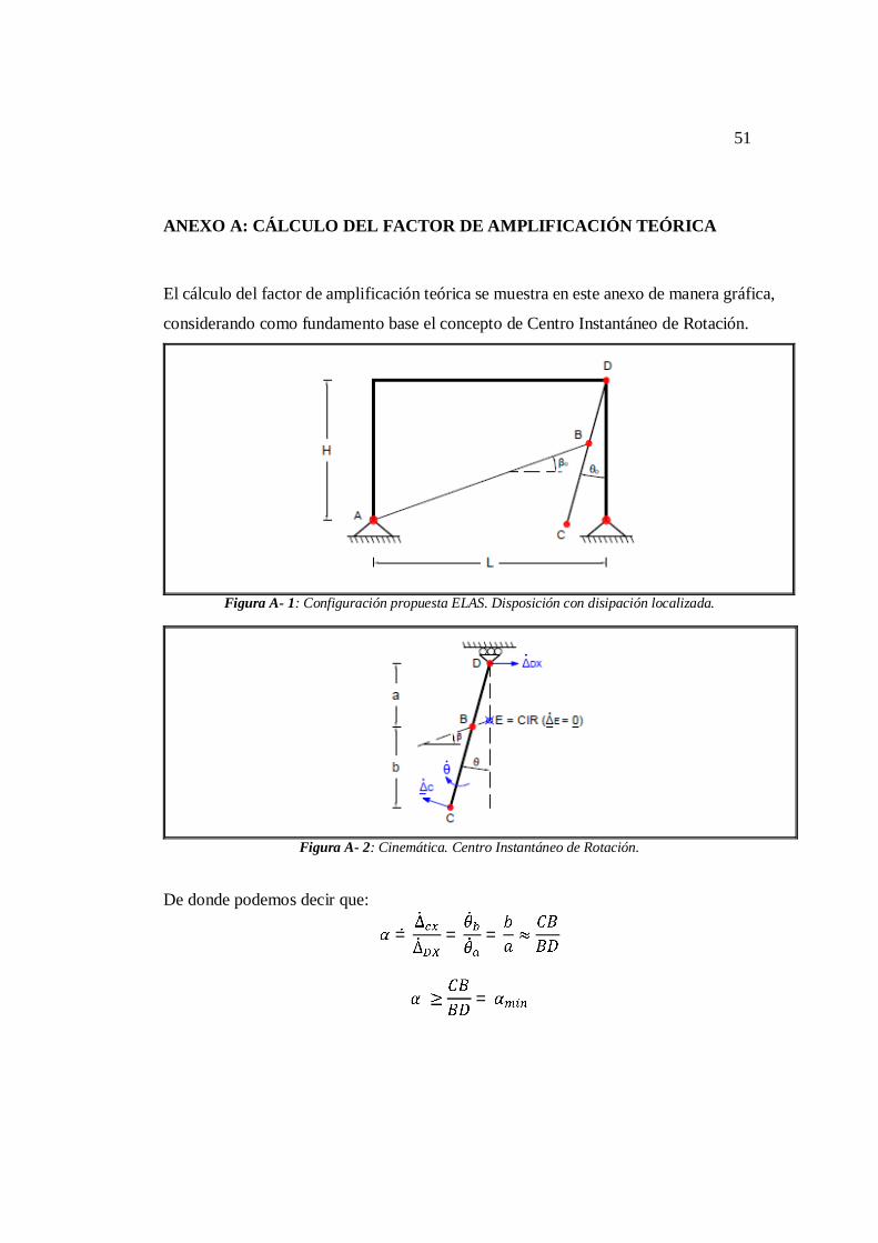
ANEXO A: CÁLCULO DEL FACTOR DE AMPLIFICACIÓN TEÓRICA
El cálculo del factor de amplificación teórica se muestra en este anexo de manera gráfica,
considerando como fundamento base el concepto de Centro Instantáneo de Rotación.
Figura A- 1: Configuración propuesta ELAS. Disposición con disipación localizada.
Figura A- 2: Cinemática. Centro Instantáneo de Rotación.
De donde podemos decir que:
= = =
=
52
ANEXO B: PUBLICACIÓN PRESENTADA N.1 Título: “AMPLIFICATION SYSTEM FOR DISTRIBUTED ENERGY DISSIPATION DEVICES.” Autores:
- Juan Sebastián Baquero Mosquera - José Luis Almazán Camillay - Nicolás Fernando Tapia Flores
Revista a la que se envió: Earthquake Engineering & Structural Dynamics, John Wiley & Sons Ltd.
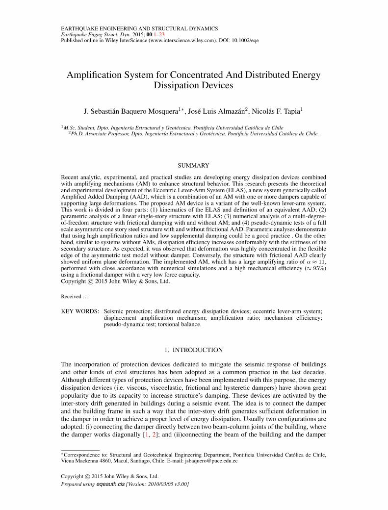
EARTHQUAKE ENGINEERING AND STRUCTURAL DYNAMICSEarthquake Engng Struct. Dyn. 2015; 00:1–23Published online in Wiley InterScience (www.interscience.wiley.com). DOI: 10.1002/eqe
Amplification System for Concentrated And Distributed EnergyDissipation Devices
J. Sebastian Baquero Mosquera1∗, Jose Luis Almazan2, Nicolas F. Tapia1
1M.Sc. Student, Dpto. Ingenierıa Estructural y Geotecnica. Pontificia Universidad Catolica de Chile2Ph.D. Associate Professor, Dpto. Ingenierıa Estructural y Geotecnica. Pontificia Universidad Catolica de Chile.
SUMMARY
Recent analytic, experimental, and practical studies are developing energy dissipation devices combinedwith amplifying mechanisms (AM) to enhance structural behavior. This research presents the theoreticaland experimental development of the Eccentric Lever-Arm System (ELAS), a new system generically calledAmplified Added Damping (AAD), which is a combination of an AM with one or more dampers capable ofsupporting large deformations. The proposed AM device is a variant of the well-known lever-arm system.This work is divided in four parts: (1) kinematics of the ELAS and definition of an equivalent AAD; (2)parametric analysis of a linear single-story structure with ELAS; (3) numerical analysis of a multi-degree-of-freedom structure with frictional damping with and without AM; and (4) pseudo-dynamic tests of a fullscale asymmetric one story steel structure with and without frictional AAD. Parametric analyses demonstratethat using high amplification ratios and low supplemental damping could be a good practice . On the otherhand, similar to systems without AMs, dissipation efficiency increases conformably with the stiffness of thesecondary structure. As expected, it was observed that deformation was highly concentrated in the flexibleedge of the asymmetric test model without damper. Conversely, the structure with frictional AAD clearlyshowed uniform plane deformation. The implemented AM, which has a large amplifying ratio of α ≈ 11,performed with close accordance with numerical simulations and a high mechanical efficiency (≈ 95%)using a frictional damper with a very low force capacity.Copyright c© 2015 John Wiley & Sons, Ltd.
Received . . .
KEY WORDS: Seismic protection; distributed energy dissipation devices; eccentric lever-arm system;displacement amplification mechanism; amplification ratio; mechanism efficiency;pseudo-dynamic test; torsional balance.
1. INTRODUCTION
The incorporation of protection devices dedicated to mitigate the seismic response of buildingsand other kinds of civil structures has been adopted as a common practice in the last decades.Although different types of protection devices have been implemented with this purpose, the energydissipation devices (i.e. viscous, viscoelastic, frictional and hysteretic dampers) have shown greatpopularity due to its capacity to increase structure’s damping. These devices are activated by theinter-story drift generated in buildings during a seismic event. The idea is to connect the damperand the building frame in such a way that the inter-story drift generates sufficient deformation inthe damper in order to achieve a proper level of energy dissipation. Usually two configurations areadopted: (i) connecting the damper directly between two beam-column joints of the building, wherethe damper works diagonally [1, 2]; and (ii)connecting the beam of the building and the damper
∗Correspondence to: Structural and Geotechnical Engineering Department, Pontificia Universidad Catolica de Chile,Vicua Mackenna 4860, Macul, Santiago, Chile. E-mail: [email protected]
Copyright c© 2015 John Wiley & Sons, Ltd.Prepared using eqeauth.cls [Version: 2010/03/05 v3.00]
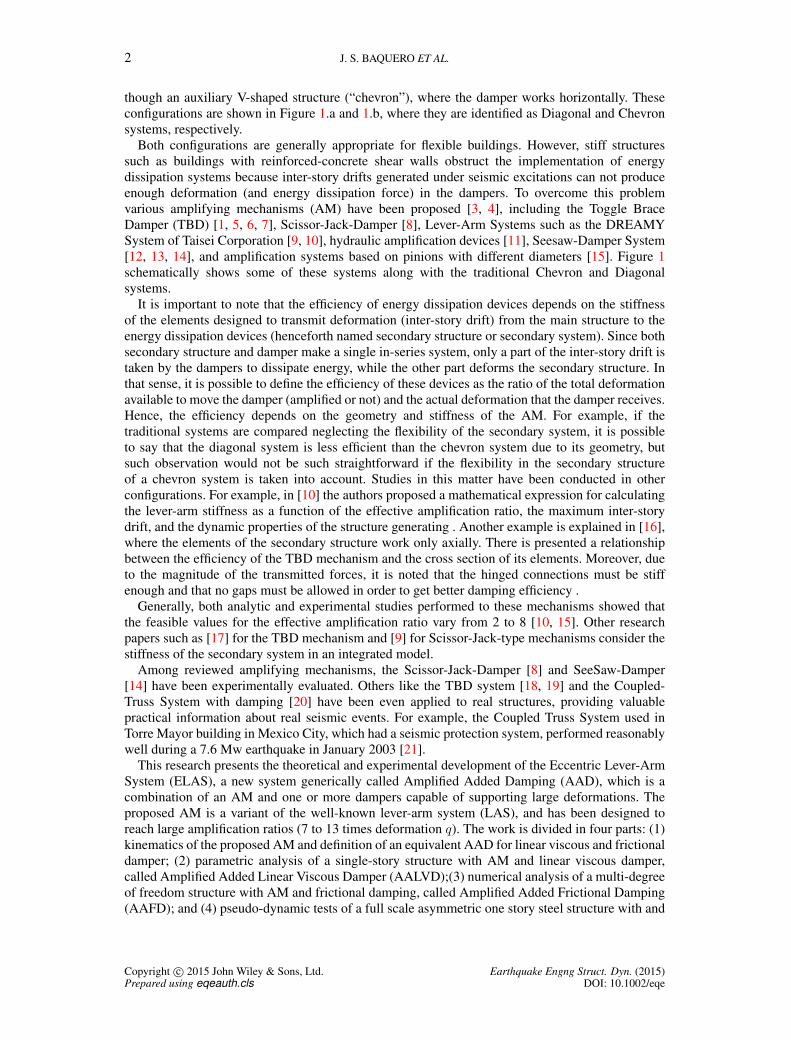
2 J. S. BAQUERO ET AL.
though an auxiliary V-shaped structure (“chevron”), where the damper works horizontally. Theseconfigurations are shown in Figure 1.a and 1.b, where they are identified as Diagonal and Chevronsystems, respectively.
Both configurations are generally appropriate for flexible buildings. However, stiff structuressuch as buildings with reinforced-concrete shear walls obstruct the implementation of energydissipation systems because inter-story drifts generated under seismic excitations can not produceenough deformation (and energy dissipation force) in the dampers. To overcome this problemvarious amplifying mechanisms (AM) have been proposed [3, 4], including the Toggle BraceDamper (TBD) [1, 5, 6, 7], Scissor-Jack-Damper [8], Lever-Arm Systems such as the DREAMYSystem of Taisei Corporation [9, 10], hydraulic amplification devices [11], Seesaw-Damper System[12, 13, 14], and amplification systems based on pinions with different diameters [15]. Figure 1schematically shows some of these systems along with the traditional Chevron and Diagonalsystems.
It is important to note that the efficiency of energy dissipation devices depends on the stiffnessof the elements designed to transmit deformation (inter-story drift) from the main structure to theenergy dissipation devices (henceforth named secondary structure or secondary system). Since bothsecondary structure and damper make a single in-series system, only a part of the inter-story drift istaken by the dampers to dissipate energy, while the other part deforms the secondary structure. Inthat sense, it is possible to define the efficiency of these devices as the ratio of the total deformationavailable to move the damper (amplified or not) and the actual deformation that the damper receives.Hence, the efficiency depends on the geometry and stiffness of the AM. For example, if thetraditional systems are compared neglecting the flexibility of the secondary system, it is possibleto say that the diagonal system is less efficient than the chevron system due to its geometry, butsuch observation would not be such straightforward if the flexibility in the secondary structureof a chevron system is taken into account. Studies in this matter have been conducted in otherconfigurations. For example, in [10] the authors proposed a mathematical expression for calculatingthe lever-arm stiffness as a function of the effective amplification ratio, the maximum inter-storydrift, and the dynamic properties of the structure generating . Another example is explained in [16],where the elements of the secondary structure work only axially. There is presented a relationshipbetween the efficiency of the TBD mechanism and the cross section of its elements. Moreover, dueto the magnitude of the transmitted forces, it is noted that the hinged connections must be stiffenough and that no gaps must be allowed in order to get better damping efficiency .
Generally, both analytic and experimental studies performed to these mechanisms showed thatthe feasible values for the effective amplification ratio vary from 2 to 8 [10, 15]. Other researchpapers such as [17] for the TBD mechanism and [9] for Scissor-Jack-type mechanisms consider thestiffness of the secondary system in an integrated model.
Among reviewed amplifying mechanisms, the Scissor-Jack-Damper [8] and SeeSaw-Damper[14] have been experimentally evaluated. Others like the TBD system [18, 19] and the Coupled-Truss System with damping [20] have been even applied to real structures, providing valuablepractical information about real seismic events. For example, the Coupled Truss System used inTorre Mayor building in Mexico City, which had a seismic protection system, performed reasonablywell during a 7.6 Mw earthquake in January 2003 [21].
This research presents the theoretical and experimental development of the Eccentric Lever-ArmSystem (ELAS), a new system generically called Amplified Added Damping (AAD), which is acombination of an AM and one or more dampers capable of supporting large deformations. Theproposed AM is a variant of the well-known lever-arm system (LAS), and has been designed toreach large amplification ratios (7 to 13 times deformation q). The work is divided in four parts: (1)kinematics of the proposed AM and definition of an equivalent AAD for linear viscous and frictionaldamper; (2) parametric analysis of a single-story structure with AM and linear viscous damper,called Amplified Added Linear Viscous Damper (AALVD);(3) numerical analysis of a multi-degreeof freedom structure with AM and frictional damping, called Amplified Added Frictional Damping(AAFD); and (4) pseudo-dynamic tests of a full scale asymmetric one story steel structure with and
Copyright c© 2015 John Wiley & Sons, Ltd. Earthquake Engng Struct. Dyn. (2015)Prepared using eqeauth.cls DOI: 10.1002/eqe
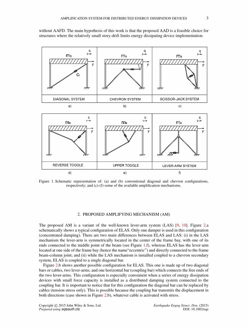
AMPLIFICATION SYSTEM FOR DISTRIBUTED ENERGY DISSIPATION DEVICES 3
without AAFD. The main hypothesis of this work is that the proposed AAD is a feasible choice forstructures where the relatively small story-drift limits energy dissipating device implementation.
Figure 1. Schematic representation of: (a) and (b) conventional diagonal and chevron configurations,respectively; and (c)-(f) some of the available amplification mechanisms.
2. PROPOSED AMPLIFYING MECHANISM (AM)
The proposed AM is a variant of the well-known lever-arm system (LAS) [9, 10]. Figure 2.aschematically shows a typical configuration of ELAS. Only one damper is used in this configuration(concentrated damping). There are two main differences between ELAS and LAS: (i) in the LASmechanism the lever-arm is symmetrically located in the center of the frame bay, with one of itsends connected to the middle point of the beam (see Figure 1.f), whereas ELAS has the lever-armlocated at one side of the frame bay (hence the name“eccentric”) and directly connected to the framebeam-column joint; and (ii) while the LAS mechanism is installed coupled to a chevron secondarysystem, ELAS is coupled to a single diagonal bar.
Figure 2.b shows another possible configuration for ELAS. This one is made up of two diagonalbars or cables, two lever-arms, and one horizontal bar (coupling bar) which connects the free ends ofthe two lever-arms. This configuration is especially convenient when a series of energy dissipationdevices with small force capacity is installed as a distributed damping system connected to thecoupling bar. It is important to notice that for this configuration the diagonal bar can be replaced bycables (tension stress only). This is possible because the coupling bar transmits the displacement inboth directions (case shown in Figure 2.b), whatever cable is activated with stress.
Copyright c© 2015 John Wiley & Sons, Ltd. Earthquake Engng Struct. Dyn. (2015)Prepared using eqeauth.cls DOI: 10.1002/eqe

4 J. S. BAQUERO ET AL.
Figure 2. Eccentric Lever-Arm System (ELAS): (a) one damper (concentrated energy dissipation); and (b)various dampers (distributed energy dissipation).
2.1. Kinematic analysis
Consider first the kinematics of the frame shown in Figure 3 provided with an ELAS for distributeddissipation with disconnected dampers (unloaded condition). If we apply a horizontal displacementq(t) to the right, the Cable 1 (active cable) rotates Lever 1 (active lever) clockwise, satisfying thefollowing equations:
L+ q(t) = ld1cosβ1(t) + asinθ1(t) (1a)H = ld1sinβ1(t) + acosθ1(t) (1b)
where H and L are the height and width of the frame, respectively; ld1 is the length of Cable 1;β1(t) is the angle between Cable 1 and the horizontal axis; and θ1(t) is the angle between Lever 1and the vertical axis (positive clockwise). In turn, Lever 1 shifts the coupling bar backwards, rotatingLever 2 clockwise, satisfying the following equations:
L+ q(t)− lp1sinθ1(t) = q(t) + lp2sinθ2(t) + lccosφ(t) (2a)H − lp1cosθ1(t) = H − lp2cosθ2(t) + lcsinφ(t) (2b)
where lp1 and lp2 are the lengths of levers 1 and 2, respectively; θ2(t) is the angle between Lever2 and the vertical axis (positive counter-clockwise); and φ(t) is the angle between the coupling-barand the horizontal axis. Cable 2 remains inactive. The situation is reversed when displacement isdirected to the left.
Equation (1) is solved for the unknowns θ1(t) and β1(t) as a function of q(t). Later, with thesolution for θ1(t), Equation (2) is solved for the unknowns θ2(t) and φ(t).
The secant and tangent amplification ratio are defined as:
αsec = −u(t)
q(t)(3a)
αtg = −dudq
= − uq
(3b)
where u(t) = q(t)− lp1sinθ1(t) is the horizontal displacement of the coupling bar. Since theelements of the mechanism are assumed perfectly rigid in this kinematic analysis, we can use theconcept of instantaneous center of rotation (ICR) to calculate αtg. Then, consider the lever shownin Figure 4. The ICR of the lever is located at the intersection of the active cable with the verticalaxis passing through the upper end of the lever. Therefore,
Copyright c© 2015 John Wiley & Sons, Ltd. Earthquake Engng Struct. Dyn. (2015)Prepared using eqeauth.cls DOI: 10.1002/eqe
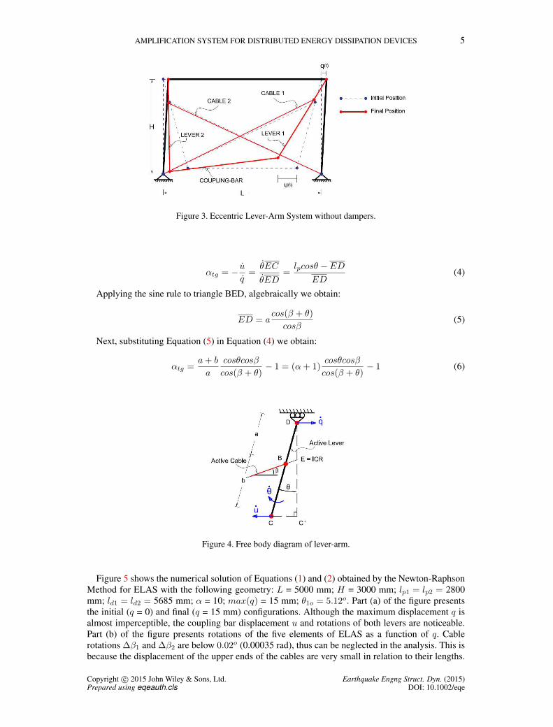
AMPLIFICATION SYSTEM FOR DISTRIBUTED ENERGY DISSIPATION DEVICES 5
Figure 3. Eccentric Lever-Arm System without dampers.
αtg = − uq
=θEC
θED=lpcosθ − ED
ED(4)
Applying the sine rule to triangle BED, algebraically we obtain:
ED = acos(β + θ)
cosβ(5)
Next, substituting Equation (5) in Equation (4) we obtain:
αtg =a+ b
a
cosθcosβ
cos(β + θ)− 1 = (α+ 1)
cosθcosβ
cos(β + θ)− 1 (6)
Figure 4. Free body diagram of lever-arm.
Figure 5 shows the numerical solution of Equations (1) and (2) obtained by the Newton-RaphsonMethod for ELAS with the following geometry: L = 5000 mm; H = 3000 mm; lp1 = lp2 = 2800mm; ld1 = ld2 = 5685 mm; α = 10; max(q) = 15 mm; θ1o = 5.12o. Part (a) of the figure presentsthe initial (q = 0) and final (q = 15 mm) configurations. Although the maximum displacement q isalmost imperceptible, the coupling bar displacement u and rotations of both levers are noticeable.Part (b) of the figure presents rotations of the five elements of ELAS as a function of q. Cablerotations ∆β1 and ∆β2 are below 0.02o (0.00035 rad), thus can be neglected in the analysis. This isbecause the displacement of the upper ends of the cables are very small in relation to their lengths.
Copyright c© 2015 John Wiley & Sons, Ltd. Earthquake Engng Struct. Dyn. (2015)Prepared using eqeauth.cls DOI: 10.1002/eqe
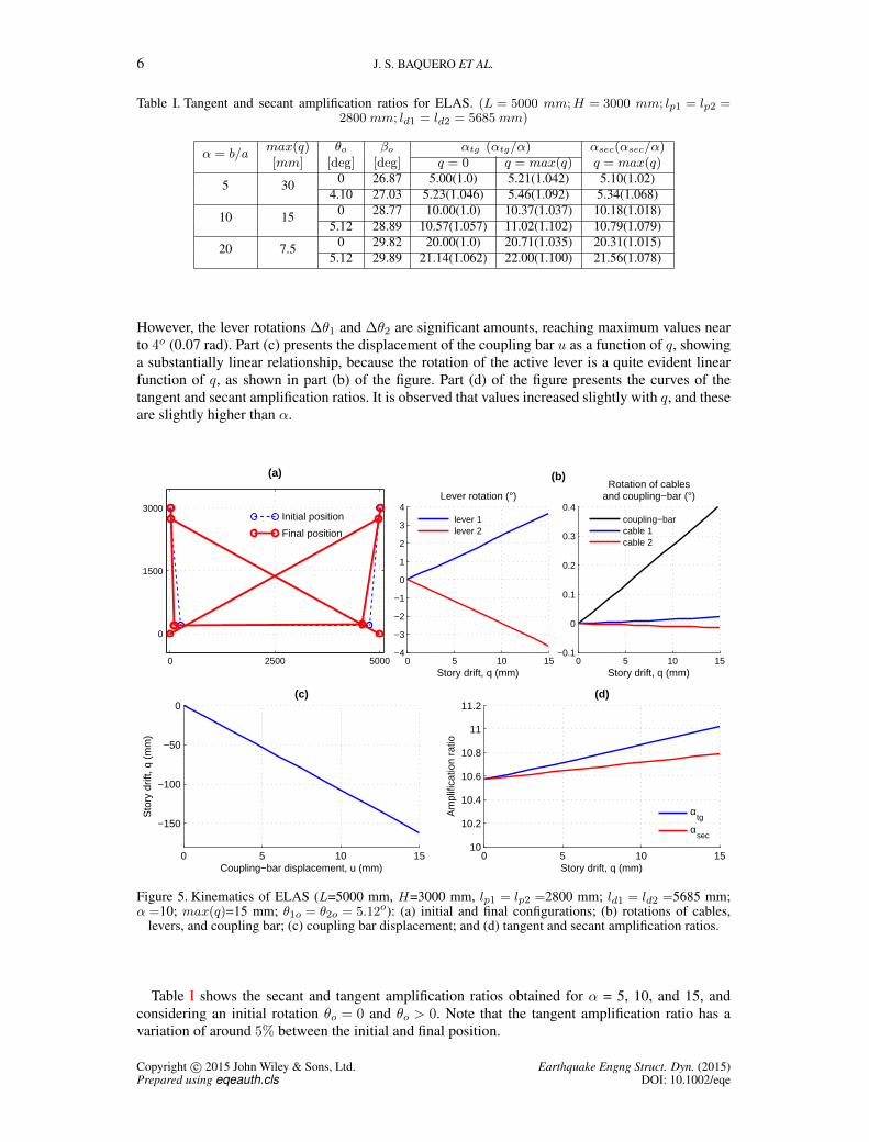
6 J. S. BAQUERO ET AL.
Table I. Tangent and secant amplification ratios for ELAS. (L = 5000 mm;H = 3000 mm; lp1 = lp2 =2800 mm; ld1 = ld2 = 5685 mm)
α = b/amax(q) θo βo αtg (αtg/α) αsec(αsec/α)[mm] [deg] [deg] q = 0 q = max(q) q = max(q)
5 30 0 26.87 5.00(1.0) 5.21(1.042) 5.10(1.02)4.10 27.03 5.23(1.046) 5.46(1.092) 5.34(1.068)
10 15 0 28.77 10.00(1.0) 10.37(1.037) 10.18(1.018)5.12 28.89 10.57(1.057) 11.02(1.102) 10.79(1.079)
20 7.5 0 29.82 20.00(1.0) 20.71(1.035) 20.31(1.015)5.12 29.89 21.14(1.062) 22.00(1.100) 21.56(1.078)
However, the lever rotations ∆θ1 and ∆θ2 are significant amounts, reaching maximum values nearto 4o (0.07 rad). Part (c) presents the displacement of the coupling bar u as a function of q, showinga substantially linear relationship, because the rotation of the active lever is a quite evident linearfunction of q, as shown in part (b) of the figure. Part (d) of the figure presents the curves of thetangent and secant amplification ratios. It is observed that values increased slightly with q, and theseare slightly higher than α.
0 2500 5000
0
1500
3000 Initial position
Final position
(a)
0 5 10 15−4
−3
−2
−1
0
1
2
3
4
Story drift, q (mm)
Lever rotation (°)
(b)
lever 1 lever 2
0 5 10 15−0.1
0
0.1
0.2
0.3
0.4
Story drift, q (mm)
Rotation of cablesand coupling−bar (°)
coupling−barcable 1cable 2
0 5 10 15
−150
−100
−50
0
Sto
ry d
rift,
q (m
m)
Coupling−bar displacement, u (mm)
(c)
0 5 10 1510
10.2
10.4
10.6
10.8
11
11.2
Story drift, q (mm)
Am
plifi
catio
n ra
tio
(d)
αtg
αsec
Figure 5. Kinematics of ELAS (L=5000 mm, H=3000 mm, lp1 = lp2 =2800 mm; ld1 = ld2 =5685 mm;α =10; max(q)=15 mm; θ1o = θ2o = 5.12o): (a) initial and final configurations; (b) rotations of cables,
levers, and coupling bar; (c) coupling bar displacement; and (d) tangent and secant amplification ratios.
Table I shows the secant and tangent amplification ratios obtained for α = 5, 10, and 15, andconsidering an initial rotation θo = 0 and θo > 0. Note that the tangent amplification ratio has avariation of around 5% between the initial and final position.
Copyright c© 2015 John Wiley & Sons, Ltd. Earthquake Engng Struct. Dyn. (2015)Prepared using eqeauth.cls DOI: 10.1002/eqe
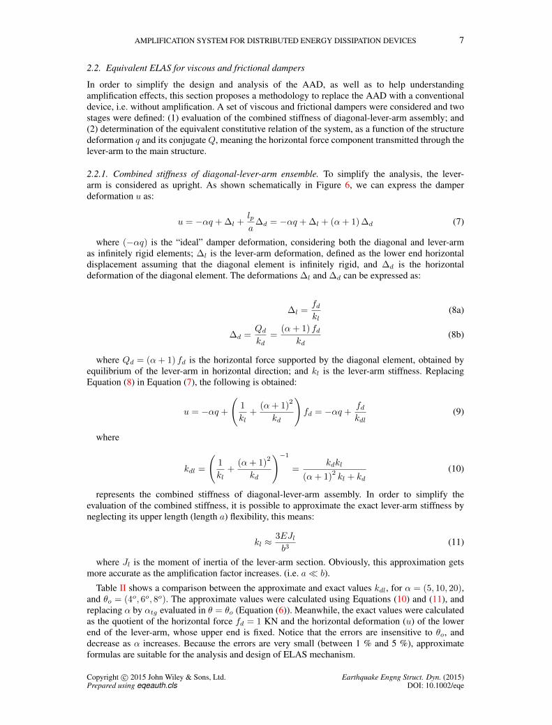
AMPLIFICATION SYSTEM FOR DISTRIBUTED ENERGY DISSIPATION DEVICES 7
2.2. Equivalent ELAS for viscous and frictional dampers
In order to simplify the design and analysis of the AAD, as well as to help understandingamplification effects, this section proposes a methodology to replace the AAD with a conventionaldevice, i.e. without amplification. A set of viscous and frictional dampers were considered and twostages were defined: (1) evaluation of the combined stiffness of diagonal-lever-arm assembly; and(2) determination of the equivalent constitutive relation of the system, as a function of the structuredeformation q and its conjugate Q, meaning the horizontal force component transmitted through thelever-arm to the main structure.
2.2.1. Combined stiffness of diagonal-lever-arm ensemble. To simplify the analysis, the lever-arm is considered as upright. As shown schematically in Figure 6, we can express the damperdeformation u as:
u = −αq + ∆l +lpa
∆d = −αq + ∆l + (α+ 1) ∆d (7)
where (−αq) is the “ideal” damper deformation, considering both the diagonal and lever-armas infinitely rigid elements; ∆l is the lever-arm deformation, defined as the lower end horizontaldisplacement assuming that the diagonal element is infinitely rigid, and ∆d is the horizontaldeformation of the diagonal element. The deformations ∆l and ∆d can be expressed as:
∆l =fdkl
(8a)
∆d =Qdkd
=(α+ 1) fd
kd(8b)
where Qd = (α+ 1) fd is the horizontal force supported by the diagonal element, obtained byequilibrium of the lever-arm in horizontal direction; and kl is the lever-arm stiffness. ReplacingEquation (8) in Equation (7), the following is obtained:
u = −αq +
(1
kl+
(α+ 1)2
kd
)fd = −αq +
fdkdl
(9)
where
kdl =
(1
kl+
(α+ 1)2
kd
)−1=
kdkl
(α+ 1)2kl + kd
(10)
represents the combined stiffness of diagonal-lever-arm assembly. In order to simplify theevaluation of the combined stiffness, it is possible to approximate the exact lever-arm stiffness byneglecting its upper length (length a) flexibility, this means:
kl ≈3EJlb3
(11)
where Jl is the moment of inertia of the lever-arm section. Obviously, this approximation getsmore accurate as the amplification factor increases. (i.e. a� b).
Table II shows a comparison between the approximate and exact values kdl, for α = (5, 10, 20),and θo = (4o, 6o, 8o). The approximate values were calculated using Equations (10) and (11), andreplacing α by αtg evaluated in θ = θo (Equation (6)). Meanwhile, the exact values were calculatedas the quotient of the horizontal force fd = 1 KN and the horizontal deformation (u) of the lowerend of the lever-arm, whose upper end is fixed. Notice that the errors are insensitive to θo, anddecrease as α increases. Because the errors are very small (between 1 % and 5 %), approximateformulas are suitable for the analysis and design of ELAS mechanism.
Copyright c© 2015 John Wiley & Sons, Ltd. Earthquake Engng Struct. Dyn. (2015)Prepared using eqeauth.cls DOI: 10.1002/eqe
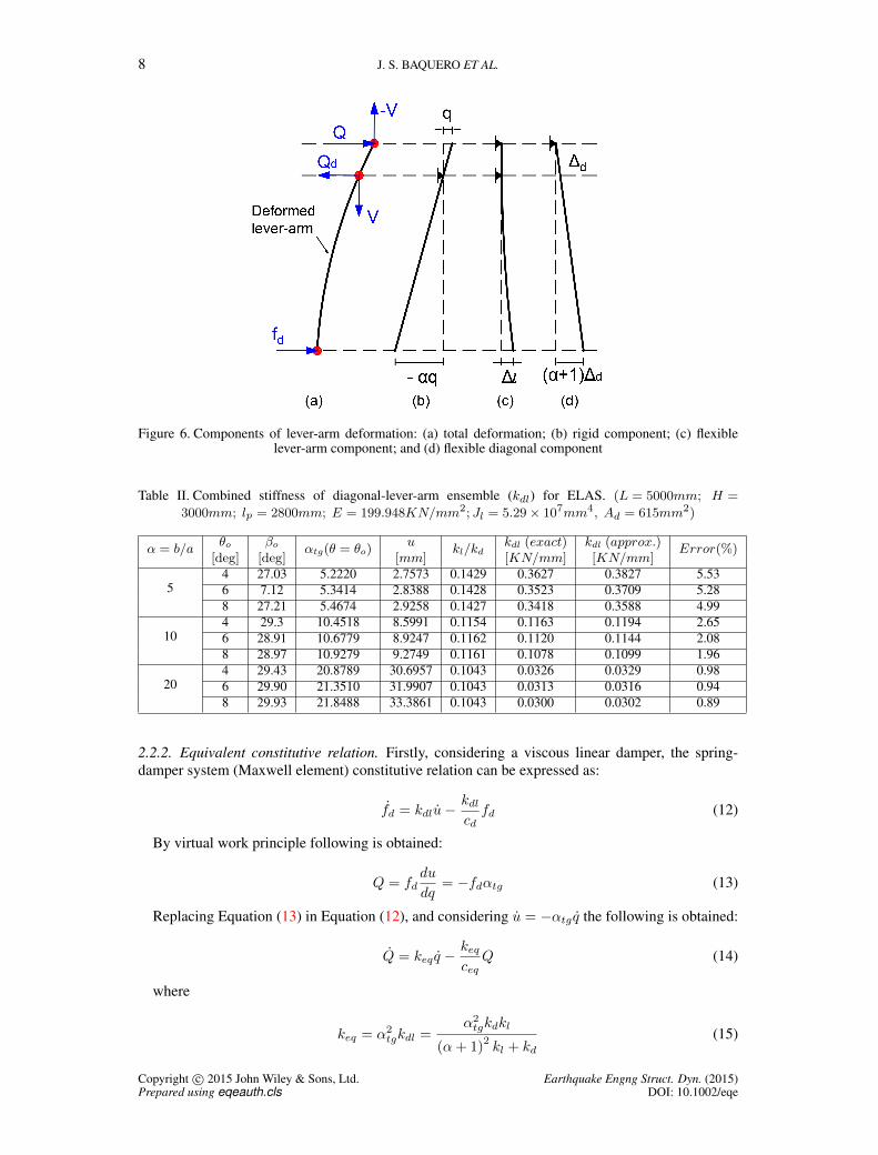
8 J. S. BAQUERO ET AL.
Figure 6. Components of lever-arm deformation: (a) total deformation; (b) rigid component; (c) flexiblelever-arm component; and (d) flexible diagonal component
Table II. Combined stiffness of diagonal-lever-arm ensemble (kdl) for ELAS. (L = 5000mm; H =
3000mm; lp = 2800mm; E = 199.948KN/mm2; Jl = 5.29 × 107mm4, Ad = 615mm2)
α = b/aθo βo αtg(θ = θo)
ukl/kd
kdl (exact) kdl (approx.)Error(%)
[deg] [deg] [mm] [KN/mm] [KN/mm]
54 27.03 5.2220 2.7573 0.1429 0.3627 0.3827 5.536 7.12 5.3414 2.8388 0.1428 0.3523 0.3709 5.288 27.21 5.4674 2.9258 0.1427 0.3418 0.3588 4.99
104 29.3 10.4518 8.5991 0.1154 0.1163 0.1194 2.656 28.91 10.6779 8.9247 0.1162 0.1120 0.1144 2.088 28.97 10.9279 9.2749 0.1161 0.1078 0.1099 1.96
204 29.43 20.8789 30.6957 0.1043 0.0326 0.0329 0.986 29.90 21.3510 31.9907 0.1043 0.0313 0.0316 0.948 29.93 21.8488 33.3861 0.1043 0.0300 0.0302 0.89
2.2.2. Equivalent constitutive relation. Firstly, considering a viscous linear damper, the spring-damper system (Maxwell element) constitutive relation can be expressed as:
fd = kdlu−kdlcdfd (12)
By virtual work principle following is obtained:
Q = fddu
dq= −fdαtg (13)
Replacing Equation (13) in Equation (12), and considering u = −αtg q the following is obtained:
Q = keq q −keqceq
Q (14)
where
keq = α2tgkdl =
α2tgkdkl
(α+ 1)2kl + kd
(15)
Copyright c© 2015 John Wiley & Sons, Ltd. Earthquake Engng Struct. Dyn. (2015)Prepared using eqeauth.cls DOI: 10.1002/eqe
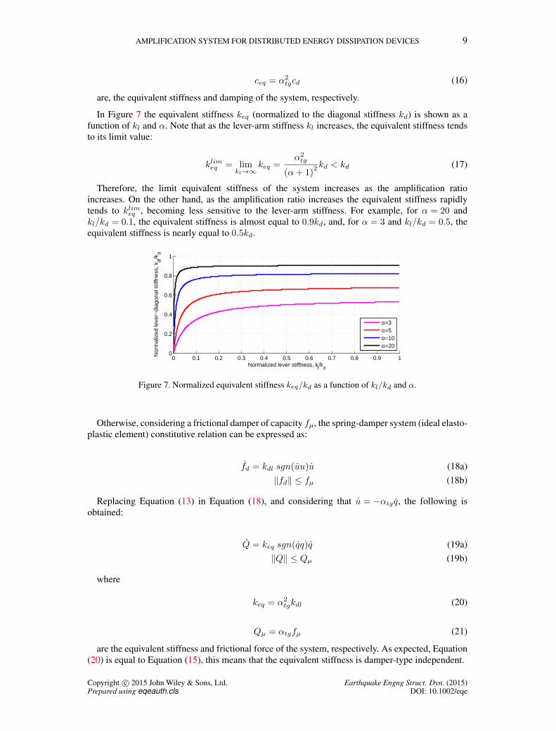
AMPLIFICATION SYSTEM FOR DISTRIBUTED ENERGY DISSIPATION DEVICES 9
ceq = α2tgcd (16)
are, the equivalent stiffness and damping of the system, respectively.
In Figure 7 the equivalent stiffness keq (normalized to the diagonal stiffness kd) is shown as afunction of kl and α. Note that as the lever-arm stiffness kl increases, the equivalent stiffness tendsto its limit value:
klimeq = limkl→∞
keq =α2tg
(α+ 1)2 kd < kd (17)
Therefore, the limit equivalent stiffness of the system increases as the amplification ratioincreases. On the other hand, as the amplification ratio increases the equivalent stiffness rapidlytends to klimeq , becoming less sensitive to the lever-arm stiffness. For example, for α = 20 andkl/kd = 0.1, the equivalent stiffness is almost equal to 0.9kd, and, for α = 3 and kl/kd = 0.5, theequivalent stiffness is nearly equal to 0.5kd.
0 0.1 0.2 0.3 0.4 0.5 0.6 0.7 0.8 0.9 10
0.2
0.4
0.6
0.8
1
Normalized lever stiffness, kl/k
d
Nor
mal
ized
leve
r−di
agon
al s
tiffn
ess,
kdl
/kd
α=3α=5α=10α=20
Figure 7. Normalized equivalent stiffness keq/kd as a function of kl/kd and α.
Otherwise, considering a frictional damper of capacity fµ, the spring-damper system (ideal elasto-plastic element) constitutive relation can be expressed as:
fd = kdl sgn(uu)u (18a)‖fd‖ ≤ fµ (18b)
Replacing Equation (13) in Equation (18), and considering that u = −αtg q, the following isobtained:
Q = keq sgn(qq)q (19a)‖Q‖ ≤ Qµ (19b)
where
keq = α2tgkdl (20)
Qµ = αtgfµ (21)
are the equivalent stiffness and frictional force of the system, respectively. As expected, Equation(20) is equal to Equation (15), this means that the equivalent stiffness is damper-type independent.
Copyright c© 2015 John Wiley & Sons, Ltd. Earthquake Engng Struct. Dyn. (2015)Prepared using eqeauth.cls DOI: 10.1002/eqe
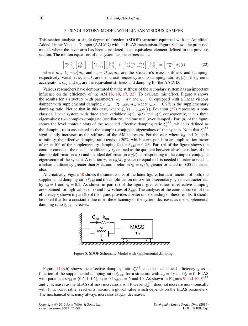
10 J. S. BAQUERO ET AL.
3. SINGLE STORY MODEL WITH LINEAR VISCOUS DAMPER
This section analyses a single-degree of freedom (SDOF) structure equipped with an AmplifiedAdded Linear Viscous Damper (AALVD) with an ELAS mechanism. Figure 8 shows the proposedmodel, where the lever-arm has been considered as an equivalent element defined in the previoussection. The motion equations of the system can be expressed as:[
ms 00 0
][q(t)u(t)
]+[cs 00 ceq
][q(t)u(t)
]+[ks+keq −keq−keq −keq
][q(t)u(t)
]=[−ms0
]xg(t) (22)
where ms, ks = ω2sms and cs = 2ξsωsms are the structure’s mass, stiffness and damping,
respectively. Variables ωs and ξs are the natural frequency and its damping ratio; xg(t) is the groundacceleration; keq and ceq are the equivalent stiffness and damping for the AALVD.
Various researchers have demonstrated that the stiffness of the secondary system has an importantinfluence on the efficiency of the AM [8, 10, 17, 22]. To evaluate this effect, Figure 9 showsthe results for a structure with parameters: ωs = 4π and ξs = 0, equipped with a linear viscousdamper with supplemental damping cadd = 2ξaddωsms, where ξadd = 0.2% is the supplementarydamping ratio. Notice that in this case, where fd(t) = caddu(t), Equation (22) represents a non-classical linear system with three state variables: q(t), q(t) and u(t) consequently, it has threeeigenvalues: two complex-conjugate (oscillatory) and one real (over damped). Part (a) of the figureshows the level contour plots of the so-called effective damping ratio ξeffd , which is defined asthe damping ratio associated to the complex-conjugate eigenvalues of the system. Note that ξeffd
significantly increases as the stiffness of the AM increases. For the case where kd and kl tendsto infinity, the effective damping ratio tends to 20%, which corresponds to an amplification factorof α2 = 100 of the supplementary damping factor ξadd = 0.2%. Part (b) of the figure shows thecontour curves of the mechanic efficiency χ, defined as the quotient between absolute values of thedamper deformation u(t) and the ideal deformation αq(t), corresponding to the complex-conjugateeigenvector of the system. A relation γd = kd/ks greater or equal to 1 is needed in order to reach amechanic efficiency greater than 80%, and a relation γl = kl/ks greater or equal to 0.05 is neededalso.
Alternatively, Figure 10 shows the same results of the latter figure, but as a function of both, thesupplemental damping ratio ξadd and the amplification ratio α for a secondary system characterizedby γd = 1 and γl = 0.1. As shown in part (a) of the figure, greater values of effective dampingare obtained for high values of α and low values of ξadd. The analysis of the contour curves of theefficiency χ shown in part (b) of the figure, provides a better understanding of these results. It shouldbe noted that for a constant value of α, the efficiency of the system decreases as the supplementaldamping ratio ξadd increases.
Figure 8. SDOF Schematic Model with supplemental damping.
Figure 11.(a,b) shows the effective damping ratio ξeffd and the mechanical efficiency χ as afunction of the supplemental damping ratio ξadd, for a structure with ωs = 4π and ξs = 0; ELASwith parameters γd = (0.5, 1, 1.5), γl = 0.1γd, α = 5 and 10. As shown in Figures 9 and 10, ξeffd
and χ increases as the ELAS stiffness increases also. However, ξeffd does not increase monotonicallywith ξadd, but it rather reaches a maximum global value which depends on the ELAS parameters.The mechanical efficiency always increases as ξadd decreases.
Copyright c© 2015 John Wiley & Sons, Ltd. Earthquake Engng Struct. Dyn. (2015)Prepared using eqeauth.cls DOI: 10.1002/eqe
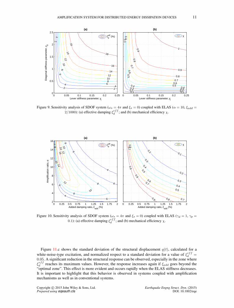
AMPLIFICATION SYSTEM FOR DISTRIBUTED ENERGY DISSIPATION DEVICES 11
2
2 2
4
44
6
6
8
8
10
10
12
12
14
14
16
16
18
Lever stiffness parameter, γl
Dia
gona
l stif
fnes
s pa
ram
eter
, γd
(a)
0 0.05 0.1 0.15 0.2 0.250
0.5
1
1.5
2
2.5
ξdeff (%)
0.1 0.10.2 0.2
0.3
0.3 0.3
0.4
0.40.4
0.5
0.5
0.6
0.6
0.7
0.7
0.8
0.8
0.9
0.9
1
Lever stiffness parameter, γl
(b)
0 0.05 0.1 0.15 0.2 0.25
χ
Figure 9. Sensitivity analysis of SDOF system (ωs = 4π and ξs = 0) coupled with ELAS (α = 10, ξadd =
2/1000): (a) effective damping ξeffd ; and (b) mechanical efficiency χ.
4
4
4
4
6
6
6
6
8
8
8
8
10
10
10
12
12
1414
16
Added damping ratio, ξadd
(%)
Am
plifi
catio
n ra
tio, α
(a)
0 0.25 0.5 0.75 1 1.25 1.5 1.75 22
4
6
8
10
12
14
16
ξdeff (%)
0.1
0.2
0.2
0.3
0.3
0.4
0.4
0.5
0.5
0.6
0.6
0.7
0.7
0.7
0.8
0.8
0.9
0.9
Added damping ratio, ξadd
(%)
(b)
0 0.25 0.5 0.75 1 1.25 1.5 1.75 2
χ
Figure 10. Sensitivity analysis of SDOF system (ωs = 4π and ξs = 0) coupled with ELAS (γd = 1, γp =
0.1): (a) effective damping ξeffd ; and (b) mechanical efficiency χ.
Figure 11.c shows the standard deviation of the structural displacement q(t), calculated for awhite-noise-type excitation, and normalized respect to a standard deviation for a value of ξeffd =0.05. A significant reduction in the structural response can be observed, especially in the zone whereξeffd reaches its maximum values. However, the response increases again if ξadd goes beyond the“optimal zone”. This effect is more evident and occurs rapidly when the ELAS stiffness decreases.It is important to highlight that this behavior is observed in systems coupled with amplificationmechanisms as well as in conventional systems.
Copyright c© 2015 John Wiley & Sons, Ltd. Earthquake Engng Struct. Dyn. (2015)Prepared using eqeauth.cls DOI: 10.1002/eqe
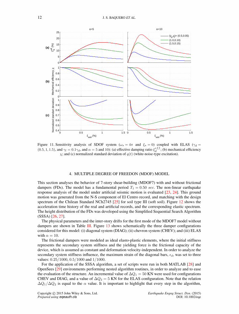
12 J. S. BAQUERO ET AL.
0
5
10
15
20
25α=5
ξ deff (
%)
(a)
α=10
(γ
d,γ
l)= (0.5,0.05)
(1.0,0.10)(1.5,0.15)
0
0.2
0.4
0.6
0.8
1
Mec
hani
cal e
ffici
ency
, χ
(b)
0 0.5 1 1.50.4
0.5
0.6
0.7
0.8
0.9
1
Nor
mal
ized
sta
ndar
t dev
iatio
n
ξadd
(%)
(c)
0 0.5 1 1.5ξ
add (%)
Figure 11. Sensitivity analysis of SDOF system (ωs = 4π and ξs = 0) coupled with ELAS (γd =
(0.5, 1, 1.5), and γl = 0.1γd, and α = 5 and 10): (a) effective damping ratio ξeffd ; (b) mechanical efficiencyχ; and (c) normalized standard deviation of q(t) (white-noise-type excitation).
4. MULTIPLE DEGREE OF FREEDON (MDOF) MODEL
This section analyses the behavior of 7-story shear-building (MDOF7) with and without frictionaldampers (FDs). The model has a fundamental period T1 = 0.50 sec. The non-linear earthquakeresponse analysis of the model under artificial seismic motion is evaluated [23, 24]. This groundmotion was generated from the N-S component of El Centro record, and matching with the designspectrum of the Chilean Standard NCh2745 [25] for soil type III (soft soil). Figure 12 shows theacceleration time history of the real and artificial records, and the corresponding elastic spectrum.The height distribution of the FDs was developed using the Simplified Sequential Search Algorithm(SSSA) [26, 27].
The physical parameters and the inter-story drifts for the first mode of the MDOF7 model withoutdampers are shown in Table III. Figure 13 shows schematically the three damper configurationsconsidered for this model: (i) diagonal system (DIAG); (ii) chevron system (CHEV); and (iii) ELASwith α = 10.
The frictional dampers were modeled as ideal elasto-plastic elements, where the initial stiffnessrepresents the secondary system stiffness and the yielding force is the frictional capacity of thedevice, which is assumed as constant and deformation velocity-independent. In order to analyze thesecondary system stiffness influence, the maximum strain of the diagonal bars, εd, was set to threevalues: 0.25/1000, 0.5/1000 and 1/1000.
For the application of the SSSA algorithm, a set of scripts were run in both MATLAB [28] andOpenSees [29] environments performing nested algorithm routines, in order to analyze and to easethe evaluation of the structure. An incremental value of ∆Q1 = 50 KN were used for configurationsCHEV and DIAG, and a value of ∆Q2 = 5 KN for the ELAS configuration. Note that the relation∆Q1/∆Q2 is equal to the α value. It is important to highlight that every step in the algorithm,
Copyright c© 2015 John Wiley & Sons, Ltd. Earthquake Engng Struct. Dyn. (2015)Prepared using eqeauth.cls DOI: 10.1002/eqe
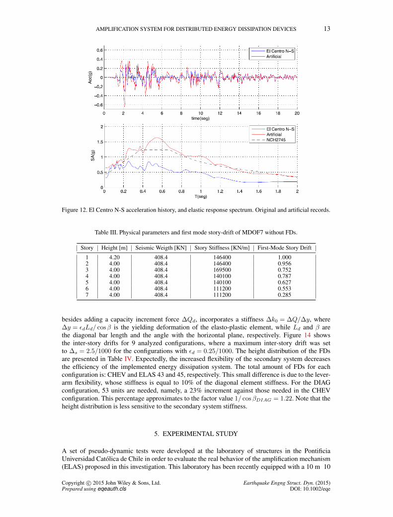
AMPLIFICATION SYSTEM FOR DISTRIBUTED ENERGY DISSIPATION DEVICES 13
Figure 12. El Centro N-S acceleration history, and elastic response spectrum. Original and artificial records.
Table III. Physical parameters and first mode story-drift of MDOF7 without FDs.
Story Height [m] Seismic Weigth [KN] Story Stiffness [KN/m] First-Mode Story Drift
1 4.20 408.4 146400 1.0002 4.00 408.4 146400 0.9563 4.00 408.4 169500 0.7524 4.00 408.4 140100 0.7875 4.00 408.4 140100 0.6276 4.00 408.4 111200 0.5537 4.00 408.4 111200 0.285
besides adding a capacity increment force ∆Qd, incorporates a stiffness ∆k0 = ∆Q/∆y, where∆y = εdLd/ cosβ is the yielding deformation of the elasto-plastic element, while Ld and β arethe diagonal bar length and the angle with the horizontal plane, respectively. Figure 14 showsthe inter-story drifts for 9 analyzed configurations, where a maximum inter-story drift was setto ∆s = 2.5/1000 for the configurations with εd = 0.25/1000. The height distribution of the FDsare presented in Table IV. Expectedly, the increased flexibility of the secondary system decreasesthe efficiency of the implemented energy dissipation system. The total amount of FDs for eachconfiguration is: CHEV and ELAS 43 and 45, respectively. This small difference is due to the lever-arm flexibility, whose stiffness is equal to 10% of the diagonal element stiffness. For the DIAGconfiguration, 53 units are needed, namely, a 23% increment against those needed in the CHEVconfiguration. This percentage approximates to the factor value 1/ cosβDIAG = 1.22. Note that theheight distribution is less sensitive to the secondary system stiffness.
5. EXPERIMENTAL STUDY
A set of pseudo-dynamic tests were developed at the laboratory of structures in the PontificiaUniversidad Catolica de Chile in order to evaluate the real behavior of the amplification mechanism(ELAS) proposed in this investigation. This laboratory has been recently equipped with a 10 m 10
Copyright c© 2015 John Wiley & Sons, Ltd. Earthquake Engng Struct. Dyn. (2015)Prepared using eqeauth.cls DOI: 10.1002/eqe

14 J. S. BAQUERO ET AL.
Figure 13. Scheme of the three frictional damper configurations considered for MDOF7 model: (a) Diagonal(DIAG); (b) Chevron (CHEV); and (c) eccentric lever arm system (ELAS).
0 1 2 3 4 5 6 7
1
2
3
4
5
6
7
Story drift (1/1000)
Sto
ry
DIAGONAL
without FDtarget
0 1 2 3 4 5 6 7Story drift (1/1000)
CHEVRON
with FD: εd=.25x10−3
with FD: εd=.50x10−3
with FD: εd=1.0x10⁻³
0 1 2 3 4 5 6 7Story drift (1/1000)
ELAS
Figure 14. Interstory drift for three configurations; DIAGONAL, CHEVRON and ELAS, after applyingSSSA Algorithm.
m in plane, and 1 m depth concrete reaction slab; a post-tensioned, L-shaped concrete reaction wallof 10 m length, 5 m height, and 0.8 m width; and a multi-axis pseudo-dynamic system (MA-PSDS),provided by the Spanish company ARIES (www.aries.com).
Copyright c© 2015 John Wiley & Sons, Ltd. Earthquake Engng Struct. Dyn. (2015)Prepared using eqeauth.cls DOI: 10.1002/eqe
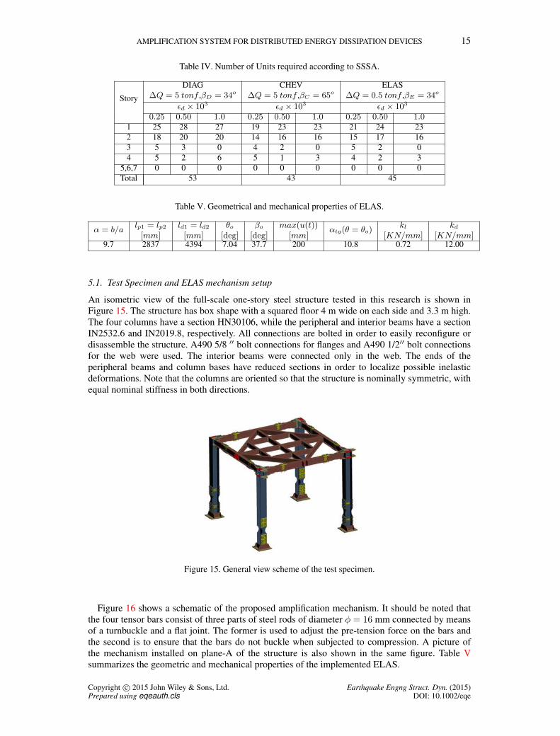
AMPLIFICATION SYSTEM FOR DISTRIBUTED ENERGY DISSIPATION DEVICES 15
Table IV. Number of Units required according to SSSA.
Story
DIAG CHEV ELAS∆Q = 5 tonf ,βD = 34o ∆Q = 5 tonf ,βC = 65o ∆Q = 0.5 tonf ,βE = 34o
εd × 103 εd × 103 εd × 103
0.25 0.50 1.0 0.25 0.50 1.0 0.25 0.50 1.01 25 28 27 19 23 23 21 24 232 18 20 20 14 16 16 15 17 163 5 3 0 4 2 0 5 2 04 5 2 6 5 1 3 4 2 3
5,6,7 0 0 0 0 0 0 0 0 0Total 53 43 45
Table V. Geometrical and mechanical properties of ELAS.
α = b/alp1 = lp2 ld1 = ld2 θo βo max(u(t))
αtg(θ = θo)kl kd
[mm] [mm] [deg] [deg] [mm] [KN/mm] [KN/mm]9.7 2837 4394 7.04 37.7 200 10.8 0.72 12.00
5.1. Test Specimen and ELAS mechanism setup
An isometric view of the full-scale one-story steel structure tested in this research is shown inFigure 15. The structure has box shape with a squared floor 4 m wide on each side and 3.3 m high.The four columns have a section HN30106, while the peripheral and interior beams have a sectionIN2532.6 and IN2019.8, respectively. All connections are bolted in order to easily reconfigure ordisassemble the structure. A490 5/8 ′′ bolt connections for flanges and A490 1/2′′ bolt connectionsfor the web were used. The interior beams were connected only in the web. The ends of theperipheral beams and column bases have reduced sections in order to localize possible inelasticdeformations. Note that the columns are oriented so that the structure is nominally symmetric, withequal nominal stiffness in both directions.
Figure 15. General view scheme of the test specimen.
Figure 16 shows a schematic of the proposed amplification mechanism. It should be noted thatthe four tensor bars consist of three parts of steel rods of diameter φ = 16 mm connected by meansof a turnbuckle and a flat joint. The former is used to adjust the pre-tension force on the bars andthe second is to ensure that the bars do not buckle when subjected to compression. A picture ofthe mechanism installed on plane-A of the structure is also shown in the same figure. Table Vsummarizes the geometric and mechanical properties of the implemented ELAS.
Copyright c© 2015 John Wiley & Sons, Ltd. Earthquake Engng Struct. Dyn. (2015)Prepared using eqeauth.cls DOI: 10.1002/eqe
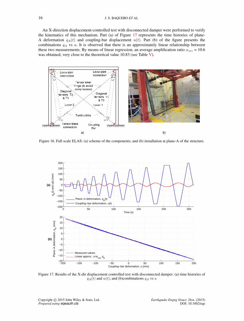
16 J. S. BAQUERO ET AL.
An X-direction displacement-controlled test with disconnected damper were performed to verifythe kinematics of this mechanism. Part (a) of Figure 17 represents the time histories of plane-A deformation qA(t) and coupling-bar displacement u(t). Part (b) of the figure presents thecombinations qA vs u. It is observed that there is an approximately linear relationship betweenthese two measurements. By means of linear regression, an average amplification ratio αsec = 10.6was obtained, very close to the theoretical value 10.83 (see Table V).
Figure 16. Full scale ELAS: (a) scheme of the components; and (b) installation at plane-A of the structure.
0 50 100 150 200 250−200
−150
−100
−50
0
50
100
150
200
Time (s)
q A(t
) an
d u(
t) (
mm
)
(a)
Plane−A deformation, qA(t)
Coupling−bar deformation, u(t)
−200 −150 −100 −50 0 50 100 150 200−20
−15
−10
−5
0
5
10
15
20
Coupling−bar deformation, u (mm)
Pla
ne−
A d
efor
mat
ion,
qA (
mm
)
(b)
Measured valuesLinear approx.: u=α
sec q
A
Figure 17. Results of the X-dir displacement controlled test with disconnected damper: (a) time histories ofqA(t) and u(t); and (b)combinations qA vs u
Copyright c© 2015 John Wiley & Sons, Ltd. Earthquake Engng Struct. Dyn. (2015)Prepared using eqeauth.cls DOI: 10.1002/eqe
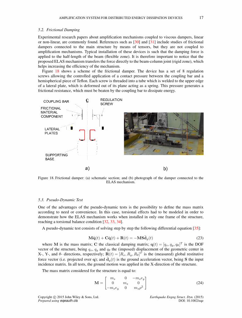
AMPLIFICATION SYSTEM FOR DISTRIBUTED ENERGY DISSIPATION DEVICES 17
5.2. Frictional Damping
Experimental research papers about amplification mechanisms coupled to viscous dampers, linearor non-linear, are commonly found. References such as [30] and [31] include studies of frictionaldampers connected to the main structure by means of tensors, but they are not coupled toamplification mechanisms. Typical installation of these devices is such that the damping force isapplied to the half-length of the beam (flexible zone). It is therefore important to notice that theproposed ELAS mechanism transfers the force directly to the beam-column joint (rigid zone), whichhelps increasing the efficiency of the mechanism.
Figure 18 shows a scheme of the frictional damper. The device has a set of 8 regulationscrews allowing the controlled application of a contact pressure between the coupling bar and ahemispherical piece of Teflon. Each screw is threaded into a tube which is welded to the upper edgeof a lateral plate, which is deformed out of its plane acting as a spring. This pressure generates africtional resistance, which must be beaten by the coupling bar to dissipate energy.
Figure 18. Frictional damper: (a) schematic section; and (b) photograph of the damper connected to theELAS mechanism.
5.3. Pseudo-Dynamic Test
One of the advantages of the pseudo-dynamic tests is the possibility to define the mass matrixaccording to need or convenience. In this case, torsional effects had to be modeled in order todemonstrate how the ELAS mechanism works when installed in only one frame of the structure,reaching a torsional balance condition [32, 33, 34].
A pseudo-dynamic test consists of solving step by step the following differential equation [35]:
Mq(t) + Cq(t) + R(t) = −MSdg(t) (23)
where M is the mass matrix; C the classical damping matrix; q(t) = [qx, qy, qθ]T is the DOF
vector of the structure, being qx, qy and qθ the (imposed) displacement of the geometric center inX-, Y-, and θ- directions, respectively; R(t) = [Rx, Ry, Rθ]
T is the (measured) global restitutiveforce vector (i.e. projected over q); and dg(t) is the ground acceleration vector, being S the inputincidence matrix. In all tests, the ground motion was applied in the X-direction of the structure.
The mass matrix considered for the structure is equal to:
M =
[ms 0 −msey0 ms 0
−msey 0 msρ2
](24)
Copyright c© 2015 John Wiley & Sons, Ltd. Earthquake Engng Struct. Dyn. (2015)Prepared using eqeauth.cls DOI: 10.1002/eqe
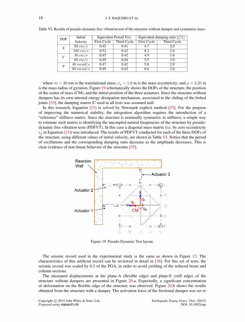
18 J. S. BAQUERO ET AL.
Table VI. Results of pseudo-dynamic free vibration test of the structure without damper and symmetric mass.
DOF Initial Equivalent Period T(s) Equivalent damping ratio ξ(%)Velocity First Cycle Third Cycle First Cycle Third Cycle
X80 cm/s 0.45 0.41 4.7 2.0160 cm/s 0.52 0.42 8.2 2.0
Y40 cm/s 0.45 0.42 4.9 1.080 cm/s 0.49 0.44 5.5 3.0
θ40 mrad/s 0.47 0.42 5.8 2.060 mrad/s 0.49 0.42 6.6 2.0
where m = 30 ton is the translational mass; ey = 1.0 m is the mass eccentricity; and ρ = 2.35 mis the mass radius of gyration. Figure 19 schematically shows the DOFs of the structure, the positionof the center of mass (CM), and the initial position of the three actuators. Since the structure withoutdampers has its own internal energy dissipation mechanism, associated to the sliding of the boltedjoints [35], the damping matrix C used in all tests was assumed null.
In this research, Equation (23) is solved by Newmark explicit method [35]. For the purposeof improving the numerical stability, the integration algorithm requires the introduction of a“reference” stiffness matrix. Since the structure is nominally symmetric in stiffness, a simple wayto estimate such matrix is identifying the uncoupled natural frequencies of the structure by pseudo-dynamic free vibration tests (PDFVT). In this case a diagonal mass matrix (i.e. by zero eccentricityey in Equation (23)) was introduced. The results of PDFVT conducted for each of the three DOFs ofthe structure, using different values of initial velocity, are shown in Table VI. Notice that the periodof oscillations and the corresponding damping ratio decrease as the amplitude decreases. This isclear evidence of non-linear behavior of the structure [35].
Figure 19. Pseudo-Dynamic Test layout.
The seismic record used in the experimental study is the same as shown in Figure 12. Thecharacteristics of this artificial record can be reviewed in detail in [36]. For this set of tests, theseismic record was scaled by 0.3 of the PGA, in order to avoid yielding of the reduced beam andcolumn sections.
The measured displacements at the plane-A (flexible edge) and plane-E (stiff edge) of thestructure without dampers are presented in Figure 20.a. Expectedly, a significant concentrationof deformation on the flexible edge of the structure was observed. Figure 20.b shows the resultsobtained from the structure with a damper. The activation force of the frictional damper was set to
Copyright c© 2015 John Wiley & Sons, Ltd. Earthquake Engng Struct. Dyn. (2015)Prepared using eqeauth.cls DOI: 10.1002/eqe
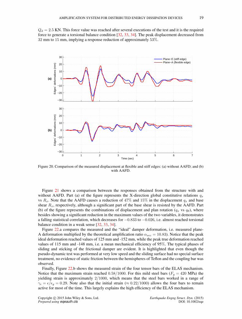
AMPLIFICATION SYSTEM FOR DISTRIBUTED ENERGY DISSIPATION DEVICES 19
Qd = 2.5 KN. This force value was reached after several executions of the test and it is the requiredforce to generate a torsional balance condition [32, 33, 34]. The peak displacement decreased from32 mm to 15 mm, implying a response reduction of approximately 53%.
−30
−20
−10
0
10
20
30E
dges
´ de
form
atio
ns (
mm
)
(a)
Plane−E (stiff edge)Plane−A (flexible edge)
0 1 2 3 4 5 6 7−30
−20
−10
0
10
20
30
Time (sec)
Edg
es´
defo
rmat
ions
(m
m)
(b)
Figure 20. Comparison of the measured displacement at flexible and stiff edges: (a) without AAFD; and (b)with AAFD.
Figure 21 shows a comparison between the responses obtained from the structure with andwithout AAFD. Part (a) of the figure represents the X-direction global constitutive relations qxvs Rx. Note that the AAFD causes a reduction of 47% and 15% in the displacement qx and baseshear Rx, respectively, although a significant part of the base shear is resisted by the AAFD. Part(b) of the figure represents the combinations of displacement and plan rotation (qx vs qθ), wherebesides showing a significant reduction in the maximum values of the two variables, it demonstratesa falling statistical correlation, which decreases for −0.833 to −0.026, i.e. almost reached torsionalbalance condition in a weak sense [32, 33, 34].
Figure 22.a compares the measured and the “ideal” damper deformation, i.e. measured plane-A deformation multiplied by the theoretical amplification ratio αsec = 10.83). Notice that the peakideal deformation reached values of 125 mm and -152 mm, while the peak true deformation reachedvalues of 115 mm and -148 mm, i.e. a mean mechanical efficiency of 95%. The typical phases ofsliding and sticking of the frictional damper are evident. It is highlighted that even though thepseudo-dynamic test was performed at very low speed and the sliding surface had no special surfacetreatment, no evidence of static friction between the hemispheres of Teflon and the coupling bar wasobserved.
Finally, Figure 22.b shows the measured strain of the four tensor bars of the ELAS mechanism.Notice that the maximum strain reached 0.58/1000. For this mild steel bars (Fy = 420 MPa) theyielding strain is approximately 2/1000, which means that the steel bars worked in a range ofγε = ε/εy = 0.29. Note also that the initial strain (≈ 0.22/1000) allows the four bars to remainactive for most of the time. This largely explains the high efficiency of the ELAS mechanism.
Copyright c© 2015 John Wiley & Sons, Ltd. Earthquake Engng Struct. Dyn. (2015)Prepared using eqeauth.cls DOI: 10.1002/eqe
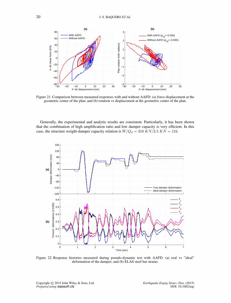
20 J. S. BAQUERO ET AL.
−30 −20 −10 0 10 20 30−80
−60
−40
−20
0
20
40
60
80
X−dir dispacement (mm)
X−
dir
shea
r fo
rce
(KN
)
(a)
With AAFDWithout AAFD
−30 −20 −10 0 10 20 30−3
−2
−1
0
1
2
3
X−dir dispacement (mm)
Pla
n ro
tatio
n (m
ili−
radi
ans)
(b)
With AAFD (ρ
xθ=−0.026)
Without AAFD (ρxθ=−0.833)
Figure 21. Comparison between measured responses with and without AAFD: (a) force-displacement at thegeometric center of the plan; and (b) rotation vs displacement at the geometric center of the plan.
Generally, the experimental and analytic results are consistent. Particularly, it has been shownthat the combination of high amplification ratio and low damper capacity is very efficient. In thiscase, the structure weight-damper capacity relation is W/Qd = 310 KN/2.5 KN = 124.
−160
−120
−80
−40
0
40
80
120
160
Dam
per
defo
rmat
ion
(mm
)
(a)
True damper deformationIdeal damper deformation
0 1 2 3 4 5 6 70
0.1
0.2
0.3
0.4
0.5
0.6
Time (sec)
Ten
sors
´ de
form
atio
ns (
1/10
00)
(b)
T1
T2
T3
T4
Figure 22. Response histories measured during pseudo-dynamic test with AAFD: (a) real vs ”ideal”deformation of the damper; and (b) ELAS steel bar strains.
Copyright c© 2015 John Wiley & Sons, Ltd. Earthquake Engng Struct. Dyn. (2015)Prepared using eqeauth.cls DOI: 10.1002/eqe
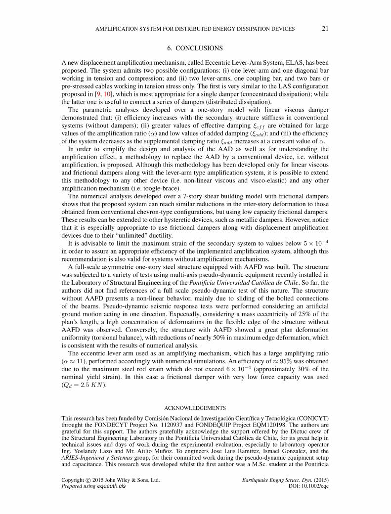
AMPLIFICATION SYSTEM FOR DISTRIBUTED ENERGY DISSIPATION DEVICES 21
6. CONCLUSIONS
A new displacement amplification mechanism, called Eccentric Lever-Arm System, ELAS, has beenproposed. The system admits two possible configurations: (i) one lever-arm and one diagonal barworking in tension and compression; and (ii) two lever-arms, one coupling bar, and two bars orpre-stressed cables working in tension stress only. The first is very similar to the LAS configurationproposed in [9, 10], which is most appropriate for a single damper (concentrated dissipation); whilethe latter one is useful to connect a series of dampers (distributed dissipation).
The parametric analyses developed over a one-story model with linear viscous damperdemonstrated that: (i) efficiency increases with the secondary structure stiffness in conventionalsystems (without dampers); (ii) greater values of effective damping ξeff are obtained for largevalues of the amplification ratio (α) and low values of added damping (ξadd); and (iii) the efficiencyof the system decreases as the supplemental damping ratio ξadd increases at a constant value of α.
In order to simplify the design and analysis of the AAD as well as for understanding theamplification effect, a methodology to replace the AAD by a conventional device, i.e. withoutamplification, is proposed. Although this methodology has been developed only for linear viscousand frictional dampers along with the lever-arm type amplification system, it is possible to extendthis methodology to any other device (i.e. non-linear viscous and visco-elastic) and any otheramplification mechanism (i.e. toogle-brace).
The numerical analysis developed over a 7-story shear building model with frictional dampersshows that the proposed system can reach similar reductions in the inter-story deformation to thoseobtained from conventional chevron-type configurations, but using low capacity frictional dampers.These results can be extended to other hysteretic devices, such as metallic dampers. However, noticethat it is especially appropriate to use frictional dampers along with displacement amplificationdevices due to their “unlimited” ductility.
It is advisable to limit the maximum strain of the secondary system to values below 5× 10⁻⁴
in order to assure an appropriate efficiency of the implemented amplification system, although thisrecommendation is also valid for systems without amplification mechanisms.
A full-scale asymmetric one-story steel structure equipped with AAFD was built. The structurewas subjected to a variety of tests using multi-axis pseudo-dynamic equipment recently installed inthe Laboratory of Structural Engineering of the Pontificia Universidad Catolica de Chile. So far, theauthors did not find references of a full scale pseudo-dynamic test of this nature. The structurewithout AAFD presents a non-linear behavior, mainly due to sliding of the bolted connectionsof the beams. Pseudo-dynamic seismic response tests were performed considering an artificialground motion acting in one direction. Expectedly, considering a mass eccentricity of 25% of theplan’s length, a high concentration of deformations in the flexible edge of the structure withoutAAFD was observed. Conversely, the structure with AAFD showed a great plan deformationuniformity (torsional balance), with reductions of nearly 50% in maximum edge deformation, whichis consistent with the results of numerical analysis.
The eccentric lever arm used as an amplifying mechanism, which has a large amplifying ratio(α ≈ 11), performed accordingly with numerical simulations. An efficiency of ≈ 95% was obtaineddue to the maximum steel rod strain which do not exceed 6× 10⁻⁴ (approximately 30% of thenominal yield strain). In this case a frictional damper with very low force capacity was used(Qd = 2.5 KN ).
ACKNOWLEDGEMENTS
This research has been funded by Comision Nacional de Investigacion Cientıfica y Tecnologica (CONICYT)throught the FONDECYT Project No. 1120937 and FONDEQUIP Project EQM120198. The authors aregrateful for this support. The authors gratefully acknowledge the support offered by the Dictuc crew ofthe Structural Engineering Laboratory in the Pontificia Universidad Catolica de Chile, for its great help intechnical issues and days of work during the experimental evaluation, especially to laboratory operatorIng. Yoslandy Lazo and Mr. Atilio Munoz. To engineers Jose Luis Ramirez, Ismael Gonzalez, and theARIES-Ingeniera y Sistemas group, for their committed work during the pseudo-dynamic equipment setupand capacitance. This research was developed whilst the first author was a M.Sc. student at the Pontificia
Copyright c© 2015 John Wiley & Sons, Ltd. Earthquake Engng Struct. Dyn. (2015)Prepared using eqeauth.cls DOI: 10.1002/eqe
22 J. S. BAQUERO ET AL.
Universidad Catolica de Chile. This author is very grateful to the funding support of the Secretarıa deEducacion Superior, Ciencia, Tecnologıa e Innovacion (SENESCYT-Ecuador) during this period of time,also, thanks the recommendations of Dr. Rafael Ruiz after reading this paper.
REFERENCES
1. Michael C Constantinou, Panos Tsopelas, Wilhelm Hammel, and Ani N. Sigaher. Toggle-Braced-Damper SeismicEnergy Dissipation Systems. Journal of Structural Engineering, (February): 105–112, 2001.
2. Ian D Aiken, Douglas K Nims, Andrew S Whittaker, and James M Kelly. Testing of Passive Energy DissipationSystems. Earthquake Spectra, 9(3), 1993.
3. T. T. Soong and Gary F. Dargush. Passive Energy Dissipation Systems in Structural Engineering. John Wiley &Sons Ltd, 1997.
4. Julian M. Londono, Simon a. Neild, and David J. Wagg. Using a damper amplification factor to increase energydissipation in structures. Engineering Structures, 84:162–171, 2015.
5. M. C. Constantinou, P. Tsopelas, and W. Hammel Testing and Modeling of an Improved Damper Configurationfor Stiff Structural Systems. State University of New York at Buffalo, Buffalo, New York, USA, 1997. TechnicalReport.
6. Jenn-shin Hwang, Yin-nan Huang, and Ya-hui Hung. Analytical and Experimental Study of Toggle-Brace-DamperSystems. Journal of Structural Engineering, 131(July):1035–1043, 2005.
7. Jenn Shin Hwang, Chun Hsiang Tsai, Shiang Jung Wang, and Yin Nan Huang. Experimental study of RC buildingstructures with supplemental viscous dampers and lightly reinforced walls. Engineering Structures, 28(13):1816–1824, 2006.
8. Ani N. Sigaher and Michael C. Constantinou. Scissor-jack-damper energy dissipation system. Earthquake Spectra,19(1):133–158, 2003.
9. N. Kani, K. Ogura, O. Tsujita, O. Hosozawa, and Y. Shinozaki. A design method and development of dampingamplifier system for passive response-controlled structure. In 10th World Conference of Earthquake Engineering,pages 4165–4170, Balkema, Rotterdam, 1992.
10. Yuri Ribakov and Andrei M. Reinhorn. Design of Amplified Structural Damping Using Optimal Considerations.Journal of Structural Engineering, 129(October):1422–1427, 2003.
11. Tracy S. K. Chung and Eddie S. S. Lam. Hydraulic Displacement Amplification System for Energy Dissipation,2004.
12. Jae-Do Kang and Tagawa Hiroshi. Seismic response of steel structures with seesaw systems using viscoelasticdampers. Earthquake Engineering & Structural Dynamics, 41:1–16, 2012.
13. Jae Do Kang and Hiroshi Tagawa. Seismic performance of steel structures with seesaw energy dissipation systemusing fluid viscous dampers. Engineering Structures, 56:431–442, 2013.
14. Jae-Do Kang and Hiroshi Tagawa. Experimental Evaluation of dynamic characteristics of seesaw energy dissipationsystems for vibration control structures. Earthquake Engineering & Structural Dynamics, 43:1889–1895, 2014.
15. Stefano Berton and John E. Bolander. Amplification System for Supplemental Damping Devices in SeismicApplications. Journal of Structural Engineering, 131(June):979–983, 2005.
16. Henry C Huang. Efficiency of the motion amplification device with viscous dampers and its application in high-risebuildings. 8(4):521–536, 2009.
17. Henry C. Huang and Robert J. McNamara. The Efficiency of the Motion Amplification Device With ViscousDamper. Technical report.
18. R J Mcnamara, C D Huang, and V Wan. Viscous-Damper with Motion Amplification Device for High Rise BuildingApplications. Advanced Technology in Structural Engineering, ASCE Struc(Philadelphia, PA, USA), 2000.
19. Stephen DeSimone and Steven Bongiorno. Long deck spans, upturned spandrels and toggle brace-dampers meetthe complex seismic requirements of the irregularly shaped steel tower for San Franciscos Four Seasons Residences.Modern Steel Construction, 2002. ISSN 00174653.
20. Andrew Ahmad Rahimian. Coupled Truss Systems with damping for seismic protection buildings, 2002.21. Douglas P Taylor. Mega brace seismic dampers for the Torre Mayor project at Mexico City. 74th Shock & Vibration
Symposium, 2003.22. Henry C Huang. Parametric study for motion amplification device with viscous damper. 13 th World Conference
on Earthquake Engineering, (Paper No. 3060), 2004.23. Jonathan Hancock, Jennie Watson-lamprey, Norman a Abrahamson, Julian J Bommer, Alexandros Markatis, and
Rishmila Mendis. An Improved Method of Matching Response Spectra of Recorded Earthquake Ground MotionUsing Wavelets. 10(1):67–89, 2006.
24. Linda Alatik and Norman Abrahamson. An improved method for nonstationary spectral matching. EarthquakeSpectra, 26(3):601–617, 2010.
25. INN-Chile. NCh. 2745 - Analisis y Diseno Sismico de Edificios con aislacion sismica. In Norma Chilena Oficial.2003.
26. D. Lopez-Garcia and T. T. Soong. Efficiency of a simple approach to damper allocation in MDOF structures.Journal of Structural Control, 9(January):19–30, 2002.
27. D. Lopez-Garcıa. A simple method for the design of optimal damper configurations in MDOF structures.Earthquake Spectra 17(3):387-398, 2001
28. MATLAB version 8.1.604 (R2013a). The MathWorks Inc., Natick - Massachusetts 201329. Frank McKenna, G. L. Fenves, M. H. Scott, and B. Jeremic. Open System for Earhquake Engineering Simulation
(OpenSees), 2000.30. Imad H. Mualla and Borislav Belev. Performance of steel frames with a new friction damper device under
earthquake excitation. Engineering Structures, 24:365–371, 2002.
Copyright c© 2015 John Wiley & Sons, Ltd. Earthquake Engng Struct. Dyn. (2015)Prepared using eqeauth.cls DOI: 10.1002/eqe
AMPLIFICATION SYSTEM FOR DISTRIBUTED ENERGY DISSIPATION DEVICES 23
31. Hyunhoon Choi and Jinkoo Kim. New installation scheme for viscoelastic dampers using cables. Canadian Journalof Civil Engineering, 37:1201–1211, 2010.
32. Juan C. de la Llera, Jose L. Almazan, and Ignacio J. Vial. Torsional balance of plan-asymmetric structures withfrictional dampers: Analytic results. Earthquake Engineering and Structural Dynamics, 34:1089–1108, 2005.
33. Ignacio Vial, Juan C. de la Llera, Jose L. Almazan, and Victor Ceballos. Torsional balance of plan-asymetricstructures with frictional dampers: Experimental Results. Earthquake Engineering & Structural Dynamics,35:1875–1898, 2006.
34. Marcos Garcıa, Juan C. de la Llera, and Jose L. Almazan. Torsional balance of plan asymmetric structures withviscoelastic dampers. Engineering Structures, 29:914–932, 2007.
35. Nicolas Felipe Tapia Flores. Desarrollo de un Sistema de Disipacion de Energıa Histeretico con Mecanismo deAmplificacion de Deformaciones. MSc thesis, Pontificia Universidad Catolica de Chile, 2015. In Spanish.
36. Juan Sebastian Baquero Mosquera. Sistema de Amplificacion para Dispositivos Distribuidos de Disipacion deEnergıa. MSc Thesis, Pontificia Universidad Catolica de Chile, 2015. In Spanish.
Copyright c© 2015 John Wiley & Sons, Ltd. Earthquake Engng Struct. Dyn. (2015)Prepared using eqeauth.cls DOI: 10.1002/eqe

53
ANEXO C: PUBLICACIÓN PRESENTADA N. 2 Título: “DEVELOPMENT OF A NOVEL COMBINED SYSTEM OF DEFORMATION AMPLIFICATION AND ADDED STIFFNESS AND DAMPING: ANALYTICAL RESULT AND FULL SCALE PSEUDO-DYNAMIC TESTS.” Autores:
- Nicolás Fernando Tapia Flores - José Luis Almazán Camillay - Juan Sebastián Baquero Mosquera
Revista a la que se envió: Engineering Structures.