sound synthesis of the geomungo using digital waveguide ... filesound synthesis of the geomungo...

석사 학위논문

Master’s Thesis

디지털도파관이론에기반한거문고의소리

합성에관한연구

Sound Synthesis of the Geomungo Using Digital Waveguide

Modeling

김 승 훈 (金承勳 Kim, Seung-hun)

문화기술대학원

Graduate School of Culture Technology

KAIST

2011



Sound Synthesis of the Geomungo Using Digital Waveguide

Modeling

Sound Synthesis of the Geomungo Using Digital

Waveguide Modeling

Advisor : Professor Yeo, Woon Seung

by

Kim, Seung-hun

Graduate School of Culture Technology

KAIST

A thesis submitted to the faculty of KAIST in partial fulfillment

of the requirements for the degree of in the Graduate School of Cul-

ture Technology . The study was conducted in accordance with Code

of Research Ethics1.

2011. 6. 1.

Approved by

Professor Yeo, Woon Seung

[Advisor]

1Declaration of Ethical Conduct in Research: I, as a graduate student of KAIST, hereby declare

that I have not committed any acts that may damage the credibility of my research. These include,

but are not limited to: falsification, thesis written by someone else, distortion of research findings

or plagiarism. I affirm that my thesis contains honest conclusions based on my own careful research

under the guidance of my thesis advisor.



김 승 훈

위 논문은 한국과학기술원 석사학위논문으로

학위논문심사위원회에서 심사 통과하였음.

2011년 6월 1일

심사위원장 여 운 승 (인)

심사위원 노 준 용 (인)

심사위원 이 교 구 (인)

MGCT

20093097

김 승 훈. Kim, Seung-hun. Sound Synthesis of the Geomungo Using Digital

Waveguide Modeling. 디지털 도파관 이론에 기반한 거문고의 소리 합성에 관

한 연구. Graduate School of Culture Technology . 2011. 77p. Advisor Prof. Yeo,

Woon Seung. Text in English.

ABSTRACT

This paper presents a sound synthesis method for the geomungo, a Korean traditional plucked-

string instrument, based on physical modeling. Commuted waveguide synthesis method is used

as a basic synthesis algorithm in this work. Recorded geomungo tones are analyzed by estimating

frequency responses and fundamental frequency curves. A synthesis model proposed here consists

of a fractional delay allpass filter, a loss filter which combines a ripple filter and an one-pole

filter, and a digital delay line. Calibration of parameters in the model is done by minimizing the

difference between the magnitude response of the designed filter and estimated losses of harmonic

partials. An time-varying model which has Lagrange interpolation FIR filter as a fractional delay

filter, time-varying loss filter and delay line, and a gain factor to preserve energy is proposed

and evaluated to generate geomungo tones which have fluctuating pitches. Gain control using a

sinusoidal function in the time-varying loss filter is also discussed. In addition, a hybrid-modal

synthesis model which synthesizes the signal with the resonators at low frequencies and with

the digital waveguide model at high frequencies is proposed. Finally, real-time sound synthesis

application is implemented based on The Synthesis toolkit(STK). The former shows that physical

modeling based on digital waveguide theory is an effective method to synthesize geomungo sounds.

i

Contents

Abstract . . . . . . . . . . . . . . . . . . . . . . . . . . . . . . . . . . . i

Contents . . . . . . . . . . . . . . . . . . . . . . . . . . . . . . . . . . . ii

Chapter 1. Introduction 1

1.1 the geomungo . . . . . . . . . . . . . . . . . . . . . . . . . . . 4

1.1.1 Structure . . . . . . . . . . . . . . . . . . . . . . . . . 5

1.1.2 Technique . . . . . . . . . . . . . . . . . . . . . . . . . 5

1.2 Background theory . . . . . . . . . . . . . . . . . . . . . . . . 6

1.2.1 Physical modeling . . . . . . . . . . . . . . . . . . . . 6

1.2.2 MSW algorithm . . . . . . . . . . . . . . . . . . . . . 7

1.2.3 Karplus-Strong(KS) algorithm . . . . . . . . . . . . 8

1.2.4 Digital Waveguide Theory . . . . . . . . . . . . . . . 9

1.2.5 Commuted Waveguide Synthesis . . . . . . . . . . . 13

1.2.6 Fractional delay filter . . . . . . . . . . . . . . . . . . 14

1.3 Related work . . . . . . . . . . . . . . . . . . . . . . . . . . . 19

1.3.1 Physical modeling of plucked string instruments . . 19

1.3.2 Physical modeling of asian string instruments . . . 20

Chapter 2. Analysis 21

2.1 Extraction of geomungo tones . . . . . . . . . . . . . . . . . 21

2.2 Frequency response . . . . . . . . . . . . . . . . . . . . . . . 21

2.3 Estimation of fundamental frequency . . . . . . . . . . . . . 23

ii

Chapter 3. General sound synthesis model 28

3.1 Synthesis model . . . . . . . . . . . . . . . . . . . . . . . . . 28

3.1.1 Loss filter . . . . . . . . . . . . . . . . . . . . . . . . . 28


3.1.3 Delay line . . . . . . . . . . . . . . . . . . . . . . . . . 31

3.2 Calibration . . . . . . . . . . . . . . . . . . . . . . . . . . . . 31

3.2.1 Estimation of the frequency-dependent loss . . . . . 31

3.2.2 Design of loss filter . . . . . . . . . . . . . . . . . . . 33

3.2.3 Design of allpass filter and delay line . . . . . . . . 35

3.2.4 Inverse filtering . . . . . . . . . . . . . . . . . . . . . 37

3.3 Synthesis . . . . . . . . . . . . . . . . . . . . . . . . . . . . . . 38

Chapter 4. Time-varying synthesis model 41

4.1 Synthesis model . . . . . . . . . . . . . . . . . . . . . . . . . 41

4.1.1 Loss filter . . . . . . . . . . . . . . . . . . . . . . . . . 42


4.1.3 Delay line . . . . . . . . . . . . . . . . . . . . . . . . . 43

4.2 Calibration . . . . . . . . . . . . . . . . . . . . . . . . . . . . 43

4.3 Synthesis . . . . . . . . . . . . . . . . . . . . . . . . . . . . . . 45

Chapter 5. Hybrid modal-waveguide synthesis model 51

5.1 Synthesis model . . . . . . . . . . . . . . . . . . . . . . . . . 51

5.1.1 Resonator . . . . . . . . . . . . . . . . . . . . . . . . . 51

5.2 Calibration . . . . . . . . . . . . . . . . . . . . . . . . . . . . 53

5.2.1 Extraction of harmonic partials . . . . . . . . . . . . 53

5.2.2 Estimation of decay rate and initial magnitude . . 54

– iii –

5.2.3 Estimation of fundamental frequency . . . . . . . . 55

5.2.4 Estimation of gain factor . . . . . . . . . . . . . . . . 56

5.3 Synthesis . . . . . . . . . . . . . . . . . . . . . . . . . . . . . . 59

Chapter 6. Real-time sound synthesis application of the geomungo 64

6.1 Time-constant model . . . . . . . . . . . . . . . . . . . . . . 64

6.2 Time-varying model . . . . . . . . . . . . . . . . . . . . . . . 65

Chapter 7. Conclusion 69

7.1 Evaluation . . . . . . . . . . . . . . . . . . . . . . . . . . . . . 69

7.2 Summary and conclusion . . . . . . . . . . . . . . . . . . . . 70

7.3 Future works . . . . . . . . . . . . . . . . . . . . . . . . . . . 71

References 72

– iv –

Chapter 1. Introduction

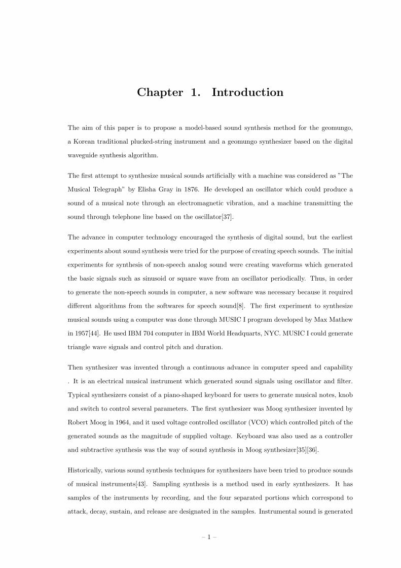
The aim of this paper is to propose a model-based sound synthesis method for the geomungo,

a Korean traditional plucked-string instrument and a geomungo synthesizer based on the digital

waveguide synthesis algorithm.

The first attempt to synthesize musical sounds artificially with a machine was considered as ”The

Musical Telegraph” by Elisha Gray in 1876. He developed an oscillator which could produce a

sound of a musical note through an electromagnetic vibration, and a machine transmitting the

sound through telephone line based on the oscillator[37].

The advance in computer technology encouraged the synthesis of digital sound, but the earliest

experiments about sound synthesis were tried for the purpose of creating speech sounds. The initial

experiments for synthesis of non-speech analog sound were creating waveforms which generated

the basic signals such as sinusoid or square wave from an oscillator periodically. Thus, in order

to generate the non-speech sounds in computer, a new software was necessary because it required

different algorithms from the softwares for speech sound[8]. The first experiment to synthesize

musical sounds using a computer was done through MUSIC I program developed by Max Mathew

in 1957[44]. He used IBM 704 computer in IBM World Headquarts, NYC. MUSIC I could generate

triangle wave signals and control pitch and duration.

Then synthesizer was invented through a continuous advance in computer speed and capability

. It is an electrical musical instrument which generated sound signals using oscillator and filter.

Typical synthesizers consist of a piano-shaped keyboard for users to generate musical notes, knob

and switch to control several parameters. The first synthesizer was Moog synthesizer invented by

Robert Moog in 1964, and it used voltage controlled oscillator (VCO) which controlled pitch of the

generated sounds as the magnitude of supplied voltage. Keyboard was also used as a controller

and subtractive synthesis was the way of sound synthesis in Moog synthesizer[35][36].

Historically, various sound synthesis techniques for synthesizers have been tried to produce sounds

of musical instruments[43]. Sampling synthesis is a method used in early synthesizers. It has

samples of the instruments by recording, and the four separated portions which correspond to

attack, decay, sustain, and release are designated in the samples. Instrumental sound is generated

– 1 –

by controlling the four portions depending on the users’ input.

Additive synthesis forms a complex waveform by adding the waveform of basic signals such as

sinusoid signal. Theoretically, it can generate any complex waveforms with many basic waveforms.

Hammond organ is a popular analog synthesizer using additive synthesis.

Frequency modulation (FM) synthesis is one of widely-used sound synthesis methods, which is

based on FM in communication systems. A basic principle of FM synthesis is that an oscillator

called modulator oscillator is modulated by another oscillator called carrier oscillator. The greatest

advantage of FM synthesis is that it can generate a complex waveform using only a small number

of oscillators. John Chowing proposed the use of FM in music at first[11]. DX7 synthesizer made

by Yamaha is a commercially successful synthesizer based on the FM synthesis[19].

These sound synthesis techniques have one thing in common: digital recordings are edited to

re-synthesize the sound. They controls the input signal and function to get a desired spectrum.

On the other hand, physical modeling synthesis is based on mathematical models of the physical

acoustics. A small change in producing sounds can be controlled by adjusting parameters, so

it does not demand to record all sound samples. Despite these advantage, physical modeling

has been developed recently because sound synthesis methods based on the mathematical model

require high computational costs. VL1 synthesizer made by Yamaha uses digital waveguide theory

which is an improved model based on Karplus-Strong (KS) algorithm and is one of the efficient

algorithms in physical modeling[55][43].

The synthesizers discussed above are based on the hardware which consists of limitless electronic

components, so they are heavy and expensive. Thus, a software synthesizer called virtual instru-

ment was proposed as an alternative. The functions in hardware synthesizers are realized as a

computer program, so a virtual instrument is a relatively cheap and portable method to generate

the sounds of instruments. Most software synthesizers exist as plug-in programs built in digital

audio workstation (ADW) which is a computer program for users to make music by recording

and editing the sounds. By using the virtual instruments, composers can make music without

recording the sounds of real instruments. VSTi in Virtual Studio Technology (VST) developed by

Steinberg company is a popular virtual instrument.

These software synthesizers can generate the sounds of various western musical instruments. How-

ever, there is lack of the programs for Korean traditional musical instruments. VST for Korean

traditional music developed by Hanyang University is the only known virtual Korean traditional

– 2 –

instruments so far, but it cannot create the instrument sounds due to the unique acoustical char-

acteristics such as a great pitch fluctuation since it is based on sampling synthesis.

Therefore, I want to propose an algorithm for a virtual geomungo synthesizer based on the acous-

tical analysis in this paper. As I mentioned above, it requires to record limitless samples to

establish a sound synthesis algorithm for the geomungo based on sampling synthesis, so physi-

cal modeling is a proper synthesis method which can reflect complex acoustical characteristics

of the geomungo. Especially, pitch control in the synthesis model is important because pitch of

the geomungo sounds varies more than 20Hz. Therefore, sound synthesis models based on the

acoustical analysis were proposed and the time-varying synthesis model which could create the

vibrato tones of the geomungo was implemented as a real-time sound synthesis program in order

to make a virtual instrument. This work is expected to be a foundation for sound synthesis models

of Korean traditional musical instruments and be an extension of the possibilities of composing

the geomungo musics.

This work is organized as follow. Firstly, the geomungo is introduced. Then, review of back-

ground theories such as digital waveguide synthesis, and previous works about physical modeling

of stringed instruments and asian instruments are discussed in next chapter. Analysis of geomungo

tones is discussed in chapter 2. Based on the analysis, a general sound synthesis model is proposed

and parameters for the model are calibrated in chapter 3. In chapter 4, the time-varying synthesis

model is proposed and the synthesized geomungo tones having fluctuant pitches are introduced.

Hybrid synthesis model for a more accurate synthesis through the control of the harmonic partials

is proposed in chapter 5. At last, in chapter 6, the real-time sound synthesis application which is

implemented based on STK is proposed.

– 3 –

1.1 the geomungo

(a)

(b)

Figure 1.1: The geomungo[38][1]

The geomungo is a string musical instruments of zither families (Fig. 1.1). It is known as a

remolded Guqin instrument imported from China before 5th century. The name comes from ”ge-

omun” (meaning ”black”) and ”go” (meaning ”zither”). It is one of three major traditional string

instruments in Silla, an ancient kingdom in Korea (the gayageum, the bipa, and the geomungo).

The volume of the sound is not loud and timbre is not gorgeous, but the sound is low and sonorous.

Thus, the geomungo was played by scholars in Chosun dynasty and was also widely used in Bud-

dhist music and court music. It has about 3 octaves pitch range which is the largest pitch range

of Korean traditional musical instruments. The geomungo is used to play bass in ensemble, but

it can play all the music range in the solo virtuoso genre called Sanjo. In addition, a percussion

sound is added because the plectrum hit the body when plucking the string strongly.

Since the 1980s, new songs for the geomungo have been composed, and technique and structure

of the instrument have been improved. However, because of lack of systematic research in unique

timbre and sound, the advantages of the geomungo are still not be taken in modern orchestral

music.

– 4 –

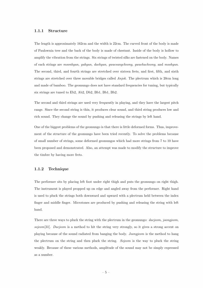
1.1.1 Structure

The length is approximately 162cm and the width is 22cm. The curved front of the body is made

of Paulownia tree and the back of the body is made of chestnut. Inside of the body is hollow to

amplify the vibration from the strings. Six strings of twisted silks are fastened on the body. Names

of each strings are moonhyun, yuhyun, daehyun, gwaesangcheong, gwaehacheong, and moohyun.

The second, third, and fourth strings are stretched over sixteen frets, and first, fifth, and sixth

strings are stretched over three movable bridges called Anjok. The plectrum which is 20cm long

and made of bamboo. The geomungo does not have standard frequencies for tuning, but typically

six strings are tuned to Eb2, Ab2, Db2, Bb1, Bb1, Bb2.

The second and third strings are used very frequently in playing, and they have the largest pitch

range. Since the second string is thin, it produces clear sound, and third string produces low and

rich sound. They change the sound by pushing and releasing the strings by left hand.

One of the biggest problems of the geomungo is that there is little deformed forms. Thus, improve-

ment of the structure of the geomungo have been tried recently. To solve the problems because

of small number of strings, some deformed geomungos which had more strings from 7 to 10 have

been proposed and demonstrated. Also, an attempt was made to modify the structure to improve

the timbre by having more frets.

1.1.2 Technique

The performer sits by placing left foot under right thigh and puts the geomungo on right thigh.

The instrument is played propped up on edge and angled away from the performer. Right hand

is used to pluck the strings both downward and upward with a plectrum held between the index

finger and middle finger. Microtones are produced by pushing and releasing the string with left

hand.

There are three ways to pluck the string with the plectrum in the geomungo: daejeom, joongjeom,

sojeom[31]. Daejeom is a method to hit the string very strongly, so it gives a strong accent on

playing because of the sound radiated from banging the body. Joongjeom is the method to hang

the plectrum on the string and then pluck the string. Sojeom is the way to pluck the string

weakly. Because of these various methods, amplitude of the sound may not be simply expressed

as a number.

– 5 –

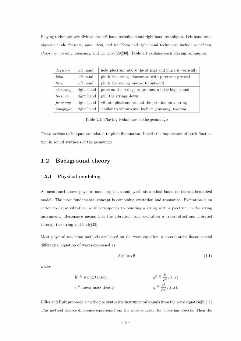
Playing techniques are divided into left hand techniques and right hand techniques. Left hand tech-

niques include daejeom, igim, tteul, and tteuldong and right hand techniques include nonghyun,

choosung, toesung, jeonsung, and chachool [29][30]. Table 1.1 explains each playing techniques.

daejeom left hand hold plectrum above the strings and pluck it vertically

igim left hand pluck the strings downward with plectrum pressed

tteul left hand pluck the strings inward to outward

choosung right hand press on the strings to produce a little high sound

toesung right hand pull the strings down

jeonsung right hand vibrate plectrum around the position on a string

nonghyun right hand similar to vibrato and include jeonsung, toesung

Table 1.1: Playing techniques of the geomungo

These various techniques are related to pitch fluctuation. It tells the importance of pitch fluctua-

tion in sound synthesis of the geomungo.

1.2 Background theory

1.2.1 Physical modeling

As mentioned above, physical modeling is a sound synthesis method based on the mathematical

model. The most fundamental concept is combining excitation and resonance. Excitation is an

action to cause vibration, so it corresponds to plucking a string with a plectrum in the string

instrument. Resonance means that the vibration from excitation is transmitted and vibrated

through the string and body[43].

Most physical modeling methods are based on the wave equation, a second-order linear partial

differential equation of waves expressed as

Ky′′ = εy (1.1)

where

K , string tension y′′ ,∂

∂ty(t, x)

ε , linear mass density y ,∂

∂xy(t, x).

Hiller and Ruiz proposed a method to synthesize instrumental sounds from the wave equation[21][22].

This method derives difference equations from the wave equation for vibrating objects. Then the

– 6 –

difference equations are solved by an iterative approximation procedure, and discrete values from

the equations represent a sound pressure wave. In this work, some conditions are necessary. First,

in order to decide the environment in which the sound produces, constants for vibrating objects

are need to specified. Second, the boundary conditions are required to limit values of the variables.

Third, the initial state such as the position in the string needs to be specified. Then, the excitation

acts as a force in the vibrating objects.

The early physical modeling synthesis methods based on the wave equation required at least one

arithmetic operation for each point on a grid the interval of which is less than half a wavelength.

They did not allow real-time sound synthesis because of a high computational cost, so an improved

algorithm was required.

1.2.2 MSW algorithm

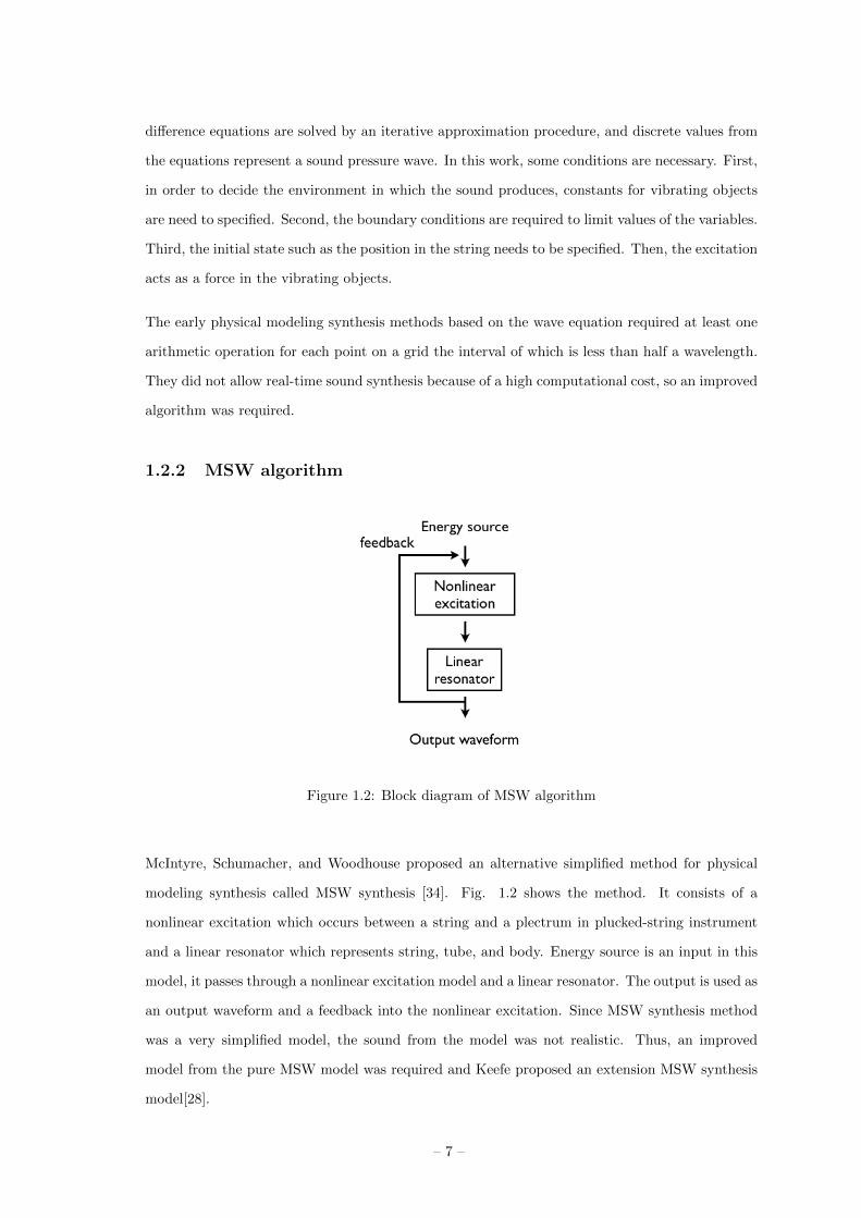
Figure 1.2: Block diagram of MSW algorithm

McIntyre, Schumacher, and Woodhouse proposed an alternative simplified method for physical

modeling synthesis called MSW synthesis [34]. Fig. 1.2 shows the method. It consists of a

nonlinear excitation which occurs between a string and a plectrum in plucked-string instrument

and a linear resonator which represents string, tube, and body. Energy source is an input in this

model, it passes through a nonlinear excitation model and a linear resonator. The output is used as

an output waveform and a feedback into the nonlinear excitation. Since MSW synthesis method

was a very simplified model, the sound from the model was not realistic. Thus, an improved

model from the pure MSW model was required and Keefe proposed an extension MSW synthesis

model[28].

– 7 –

1.2.3 Karplus-Strong(KS) algorithm

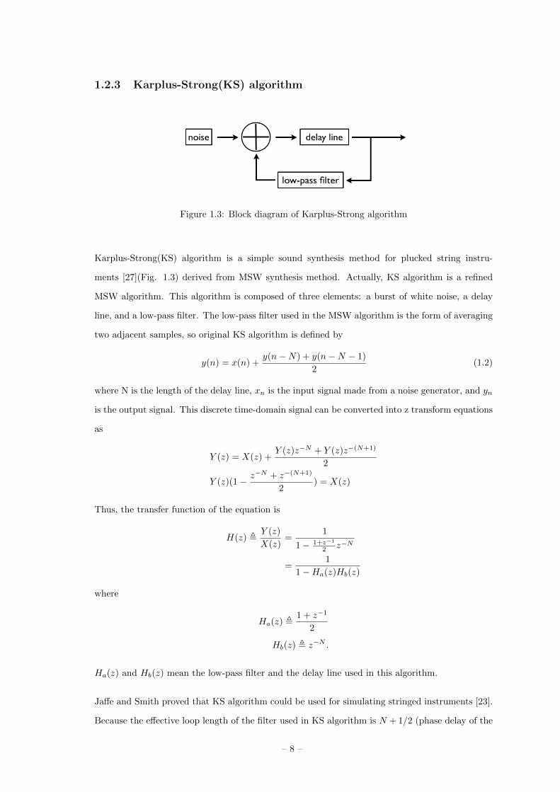
Figure 1.3: Block diagram of Karplus-Strong algorithm

Karplus-Strong(KS) algorithm is a simple sound synthesis method for plucked string instru-

ments [27](Fig. 1.3) derived from MSW synthesis method. Actually, KS algorithm is a refined

MSW algorithm. This algorithm is composed of three elements: a burst of white noise, a delay

line, and a low-pass filter. The low-pass filter used in the MSW algorithm is the form of averaging

two adjacent samples, so original KS algorithm is defined by

y(n) = x(n) +y(n−N) + y(n−N − 1)

2(1.2)

where N is the length of the delay line, xn is the input signal made from a noise generator, and yn

is the output signal. This discrete time-domain signal can be converted into z transform equations

as

Y (z) = X(z) +Y (z)z−N + Y (z)z−(N+1)

2

Y (z)(1− z−N + z−(N+1)

2) = X(z)

Thus, the transfer function of the equation is

H(z) ,Y (z)

X(z)=

1

1− 1+z−1

2 z−N

=1

1−Ha(z)Hb(z)

where

Ha(z) ,1 + z−1

2

Hb(z) , z−N .

Ha(z) and Hb(z) mean the low-pass filter and the delay line used in this algorithm.

Jaffe and Smith proved that KS algorithm could be used for simulating stringed instruments [23].

Because the effective loop length of the filter used in KS algorithm is N + 1/2 (phase delay of the

– 8 –

low-pass filter is 0.5 and of the delay line is N), so the period of the signal is Ts(N + 1/2) and

the fundamental frequency is Fs/(N + 1/2). As the magnitude spectrum of the produced signal,

harmonics which are integer multiples of the fundamental frequency exist and decay over time.

Additionally, Jaffe and Smith extended the algorithm by introducing a filter contributing a small

delay and a factor controlling decay time.

1.2.4 Digital Waveguide Theory

Introduction

Based on KS algorithm, Smith proposed a new sound synthesis method for a physical model

called digital waveguide modeling[49][50][52]. In this method, a traveling wave is simulated by a

digital delay line. Also, damping and dispersion are lumped at specific points on the assumption

that the commutativity of linear time-invariant system is valid in this system. This reduces the

computational cost enough to allow real-time sound synthesis.

Sampling

Digital waveguide modeling is based on the wave equation of the ideal vibrating string(Eq. 1.1).

The latter can be expressed by two separate traveling waves:

y(x, t) = yr(x− ct) + yl(x+ ct) (1.3)

y(t, x) = yr(t− x/c) + yl(t+ x/c) (1.4)

where yr(x− ct) is a right-going traveling wave, yl(x− ct) is a left-going traveling wave, and c is

the speed of wave. Then, this equation can be sampled with t = nT, x = mX, and X = cT :

y(nT,mX) = yr(nT −mX/c) + yl(nT +mX/c) (1.5)

= yr((n−m)T ) + yl((n+m)T )

= y+(n−m) + y−(n+m)

where

y+(n) , yr(nT ) y−(n) , yl(nT ).

In this equation, y+(n − m) can be regarded as the output of m-sample delay of y+(n), and

y−(n + m) also can be regarded as the input of m-sample delay of y−(n). Fig. 1.4 shows a

– 9 –

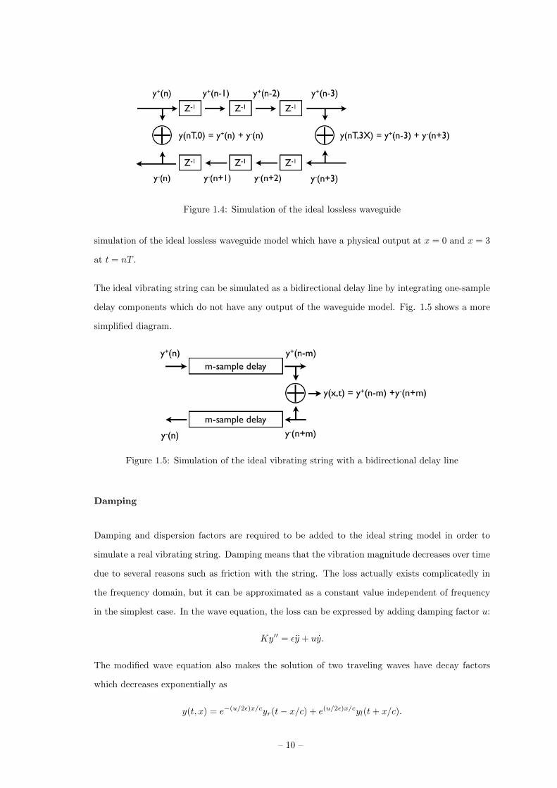
Figure 1.4: Simulation of the ideal lossless waveguide

simulation of the ideal lossless waveguide model which have a physical output at x = 0 and x = 3

at t = nT .

The ideal vibrating string can be simulated as a bidirectional delay line by integrating one-sample

delay components which do not have any output of the waveguide model. Fig. 1.5 shows a more

simplified diagram.

Figure 1.5: Simulation of the ideal vibrating string with a bidirectional delay line

Damping

Damping and dispersion factors are required to be added to the ideal string model in order to

simulate a real vibrating string. Damping means that the vibration magnitude decreases over time

due to several reasons such as friction with the string. The loss actually exists complicatedly in

the frequency domain, but it can be approximated as a constant value independent of frequency

in the simplest case. In the wave equation, the loss can be expressed by adding damping factor u:

Ky′′ = εy + uy.

The modified wave equation also makes the solution of two traveling waves have decay factors

which decreases exponentially as

y(t, x) = e−(u/2ε)x/cyr(t− x/c) + e(u/2ε)x/cyl(t+ x/c).

– 10 –

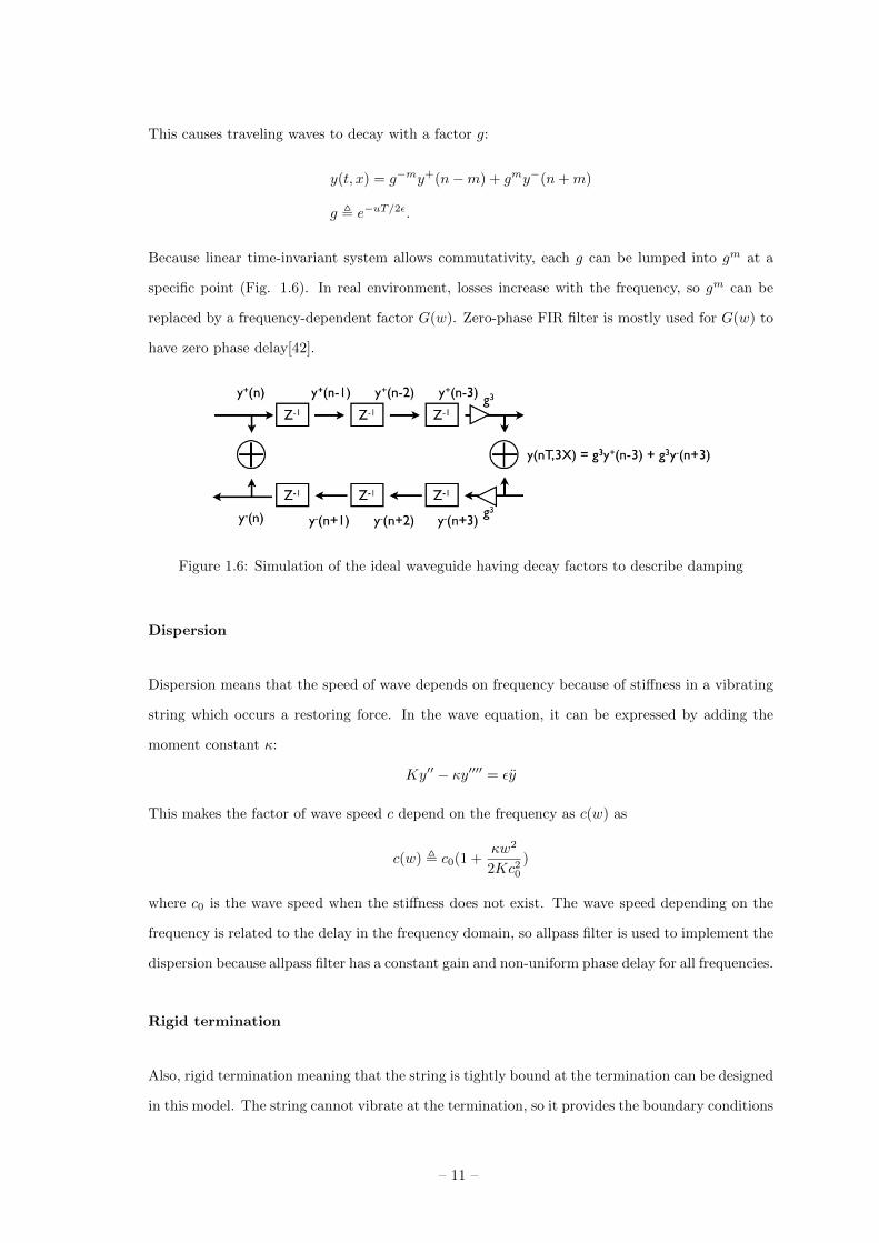
This causes traveling waves to decay with a factor g:

y(t, x) = g−my+(n−m) + gmy−(n+m)

g , e−uT/2ε.

Because linear time-invariant system allows commutativity, each g can be lumped into gm at a

specific point (Fig. 1.6). In real environment, losses increase with the frequency, so gm can be

replaced by a frequency-dependent factor G(w). Zero-phase FIR filter is mostly used for G(w) to

have zero phase delay[42].

Figure 1.6: Simulation of the ideal waveguide having decay factors to describe damping

Dispersion

Dispersion means that the speed of wave depends on frequency because of stiffness in a vibrating

string which occurs a restoring force. In the wave equation, it can be expressed by adding the

moment constant κ:

Ky′′ − κy′′′′ = εy

This makes the factor of wave speed c depend on the frequency as c(w) as

c(w) , c0(1 +κw2

2Kc20)

where c0 is the wave speed when the stiffness does not exist. The wave speed depending on the

frequency is related to the delay in the frequency domain, so allpass filter is used to implement the

dispersion because allpass filter has a constant gain and non-uniform phase delay for all frequencies.

Rigid termination

Also, rigid termination meaning that the string is tightly bound at the termination can be designed

in this model. The string cannot vibrate at the termination, so it provides the boundary conditions

– 11 –

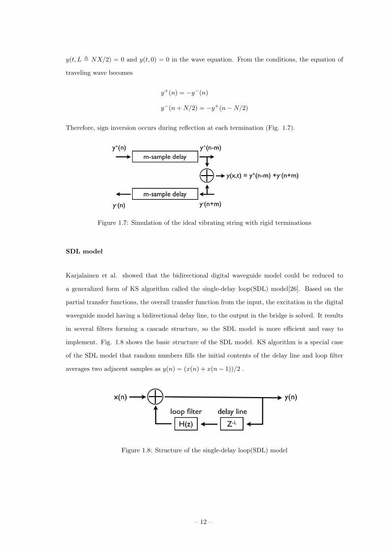
y(t, L , NX/2) = 0 and y(t, 0) = 0 in the wave equation. From the conditions, the equation of

traveling wave becomes

y+(n) = −y−(n)

y−(n+N/2) = −y+(n−N/2)

Therefore, sign inversion occurs during reflection at each termination (Fig. 1.7).

Figure 1.7: Simulation of the ideal vibrating string with rigid terminations

SDL model

Karjalainen et al. showed that the bidirectional digital waveguide model could be reduced to

a generalized form of KS algorithm called the single-delay loop(SDL) model[26]. Based on the

partial transfer functions, the overall transfer function from the input, the excitation in the digital

waveguide model having a bidirectional delay line, to the output in the bridge is solved. It results

in several filters forming a cascade structure, so the SDL model is more efficient and easy to

implement. Fig. 1.8 shows the basic structure of the SDL model. KS algorithm is a special case

of the SDL model that random numbers fills the initial contents of the delay line and loop filter

averages two adjacent samples as y(n) = (x(n) + x(n− 1))/2 .

Figure 1.8: Structure of the single-delay loop(SDL) model

– 12 –

1.2.5 Commuted Waveguide Synthesis

In plucked string instruments, plucking causes the string to vibrate and the vibration is transferred

to body through the bridge, then the sound is radiated through vibration of the air around the

body of the instrument. Thus, the plucked string instrument model has basically three components

which represent an excitation signal, a string model, and a body model (Fig. 1.9). Each of them

is expressed as a filter in the SDL model and is denoted by e(n), s(n), and b(n).

Figure 1.9: Structure of plucked string model model

In this model, the transfer function h(n) is expressed as

h(n) = e(n) ∗ s(n) ∗ b(n) (1.6)

where the asterisk denotes discrete convolution. In order to produce sounds from the model, the

filters corresponding to each component need to be approximated. However, the order of FIR filter

model for modeling the body is very high, so it requires too high computational cost to implement

a real-time sound synthesis system.

One solution for the problem is to implement the body filter with sampled impulse response of the

body of the instrument and a small number of resonators[6], but quality is not enough to provide

the features of the instrument[25].

An alternative solution called commuted waveguide synthesis was proposed by Smith. It provides

a simple and efficient synthesis model[51]. Because the instrument model can be considered as

linear time-invariant(LTI), Eq. 1.6 allows to commute the components s(n) and b(n) as

h(n) = e(n) ∗ b(n) ∗ s(n).

Then, convolution of the excitation signal x(n) and the body model b(n) gives

h(n) = x(n) ∗ s(n)

x(n) , e(n) ∗ b(n)

where x(n) can be used as the input of the string model and the string model s(n) is built

upon digital waveguide theory. In this way, the filter corresponding to the body model need not

– 13 –

be approximated. s(n) exists as a cascade form of several filters, and it can be estimated by

analyzing the gain of partials from recorded samples of the instrument. x(n) which combines the

excitation signal and the body model is stored as a form of excitation table and used to produce

sound through s(n). From digital recordings of the instruments, it can be estimated by inverse

filtering of the string model s(n).

1.2.6 Fractional delay filter

Length of the digital delay line L in the SDL model decides the fundamental frequency as

L = fs/f0

f0 = fs/L

where fs is sampling frequency and f0 is fundamental frequency. Since L is always an integer, f0

must be tuned as a number which make L an integer. It means that not all numbers can be f0.

Thus, in order to set f0 as any number, it requires an additional filter called fractional delay filter

which has a small phase delay and does not change the loop gain.

Ideal fractional delay filter has a uniform gain for all frequencies and a constant phase delay (linear

phase response). To implement the filter in digital domain, first-order allpass filter and Lagrange

interpolation FIR filter have been used[23][24].

First-order allpass filter

The transfer function of the first-order allpass filter is given as

F (z) ,C + z−1

1 + Cz−1.(1.7)

The magnitude response of the allpass filter is

G(f) = |F (ejwTs)|

=|C + e−jwTs ||1 + Ce−jwTs

=|C + 1||1 + C|

= 1.

Thus, it has unity gain for all frequencies. Then low-frequency phase delay is approximated as

– 14 –

P (f) = −∠F (ejwTs)

wTs

= − 1

wTs∠C + e−jwTs

1 + Ce−jwTs

= − 1

wTs{∠(C + e−jwTs)− ∠(1 + Ce−jwTs)}

= − 1

wTs{∠(C + cos(wTs)− j sin(wTs))− ∠(1 + C cos(wTs)− jC sin(wTs))}

= − 1

wTs{tan−1(− sin(wTs)

C + cos(wTs))− tan−1(− C sin(wTs)

1 + C cos(wTs))}.

By using Maclaurin series expansion[2], tan−1(x) can be expressed as

tan−1(x) =

∞∑n=0

(−1)n

2n+ 1x2n+1 for |x| < 1

= x− x3

3+x5

5+ · · ·

≈ x for x→ 0.

Thus, the low-frequency phase delay can be approximated as

P (f) ≈ 1

wTs(

sin(wTs)

C + cos(wTs)− C sin(wTs)

1 + C cos(wTs))

≈ (1

C + 1− C

1 + C)

=1− C1 + C.

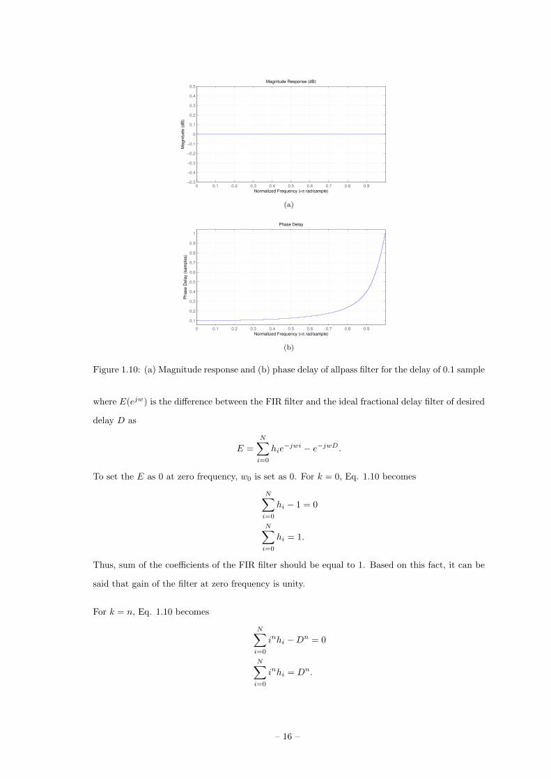
Fig. 1.10 shows the magnitude and phase delay responses of an allpass filter for 0.1 sample delay.

It has unity gain on frequency domain, and phase delay is 0.1 at low frequency.

Larange interpolation FIR filter

The equation of Lagrange interpolation FIR filter is given as

F (z) ,N∑i=0

hiz−i (1.8)

where the filter coefficients hn of desired delay D is given as

hn =

N∏k=0,k 6=n

D − kn− k

, n = 0, 1, ..., N. (1.9)

The filter is derived by the design of maximally flat filter[58]. N derivatives of an error function is

zero at the frequency w0 as

dkE(ejw)

dwk|w=w0

= 0 (1.10)

– 15 –

0 0.1 0.2 0.3 0.4 0.5 0.6 0.7 0.8 0.9−0.5

−0.4

−0.3

−0.2

−0.1

0

0.1

0.2

0.3

0.4

0.5

Normalized Frequency (×π rad/sample)

Magnitude (

dB

)

Magnitude Response (dB)

(a)

0 0.1 0.2 0.3 0.4 0.5 0.6 0.7 0.8 0.9

0.1

0.2

0.3

0.4

0.5

0.6

0.7

0.8

0.9

1


Phase D

ela

y (

sam

ple

s)

Phase Delay

(b)

Figure 1.10: (a) Magnitude response and (b) phase delay of allpass filter for the delay of 0.1 sample

where E(ejw) is the difference between the FIR filter and the ideal fractional delay filter of desired

delay D as

E =

N∑i=0

hie−jwi − e−jwD.

To set the E as 0 at zero frequency, w0 is set as 0. For k = 0, Eq. 1.10 becomes

N∑i=0

hi − 1 = 0

N∑i=0

hi = 1.

Thus, sum of the coefficients of the FIR filter should be equal to 1. Based on this fact, it can be

said that gain of the filter at zero frequency is unity.

For k = n, Eq. 1.10 becomes

N∑i=0

inhi −Dn = 0

N∑i=0

inhi = Dn.

– 16 –

To solve the Eq. 1.10, N + 1 linear equations needs to be collected as

N∑i=0

ikhi = Dk, k = 0, 1, 2, ..., N.

These can be expressed as a matrix form as

Ah = D (1.11)

where

A =

∣∣∣∣∣∣∣∣∣∣∣∣∣∣∣∣∣∣∣∣∣∣∣

00 10 20 · · · N0

01 11 21 · · · N1

02 12 22 · · · N2

· · ·

· · ·

· · ·

0N 1N 2N · · · NN

∣∣∣∣∣∣∣∣∣∣∣∣∣∣∣∣∣∣∣∣∣∣∣h =

∣∣∣∣ h0 h1 h2 · · · hN

∣∣∣∣TD =

∣∣∣∣ D0 D1 D2 · · · DN

∣∣∣∣T .Eq. 1.11 is solved as

h = A−1D

and by Cramer’s rule[56], hi is

hi =detDi

detA

where Di is the matrix which replaces ith column of A with the vector D as

Di =

∣∣∣∣∣∣∣∣∣∣∣∣∣∣∣∣∣∣∣∣∣∣∣

00 10 D0 · · · N0

01 11 D1 · · · N1

02 12 D2 · · · N2

· · ·

· · ·

· · ·

0N 1N DN · · · NN

∣∣∣∣∣∣∣∣∣∣∣∣∣∣∣∣∣∣∣∣∣∣∣

.

– 17 –

Therefore, the solution is given as a form of Eq. 1.9. For example, the filter coefficients of the

Lagrange interpolation FIR filter for N = 3 are given as

h0 = −1

6(D − 1)(D − 2)(D − 3),

h1 =1

2D(D − 2)(D − 3),

h2 =1

2D(D − 1)(D − 3),

h3 = −1

6D(D − 1)(D − 2).

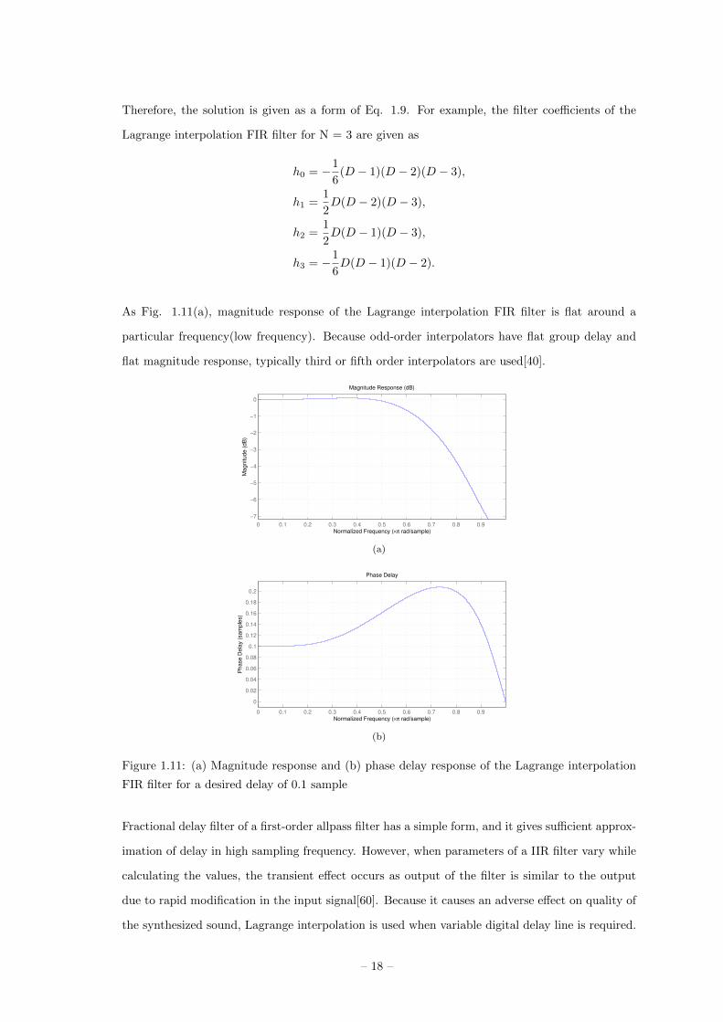
As Fig. 1.11(a), magnitude response of the Lagrange interpolation FIR filter is flat around a

particular frequency(low frequency). Because odd-order interpolators have flat group delay and

flat magnitude response, typically third or fifth order interpolators are used[40].

0 0.1 0.2 0.3 0.4 0.5 0.6 0.7 0.8 0.9

−7

−6

−5

−4

−3

−2

−1

0


Magnitude (

dB

)


(a)

0 0.1 0.2 0.3 0.4 0.5 0.6 0.7 0.8 0.9

0

0.02

0.04

0.06

0.08

0.1

0.12

0.14

0.16

0.18

0.2


Phase D

ela

y (

sam

ple

s)

Phase Delay

(b)

Figure 1.11: (a) Magnitude response and (b) phase delay response of the Lagrange interpolation

FIR filter for a desired delay of 0.1 sample

Fractional delay filter of a first-order allpass filter has a simple form, and it gives sufficient approx-

imation of delay in high sampling frequency. However, when parameters of a IIR filter vary while

calculating the values, the transient effect occurs as output of the filter is similar to the output

due to rapid modification in the input signal[60]. Because it causes an adverse effect on quality of

the synthesized sound, Lagrange interpolation is used when variable digital delay line is required.

– 18 –

1.3 Related work

Since the digital waveguide theory was proposed, many studies have been proposed to synthe-

size the sounds of various instruments. They includes various kinds of instruments such as wind

instrument[28][46][45] and bowed string instrument[64][48], but I focused on plucked string instru-

ment because the geomungo fall into the category.

1.3.1 Physical modeling of plucked string instruments

Valimaki et al. proposed a sound synthesis model based on the digital waveguide theory for

several plucked string instruments such as guitar, the banjo, the mandolin, and the kantele[59].

They adopted commuted waveguide synthesis and Lagrange interpolation for variable delay line,

and proposed a real-time synthesis method with a signal processor.

An improved model was proposed by Valimaki et al. to implement a guitar synthesizer[62]. Instead

of the cascade model of commuted waveguide synthesis, they used the parallel model in which two

resonators producing low resonances were separated from the excitation signal. This method could

reduce the length of the excitation signal and parametrize the low body resonances.

Piano has a similar structure to other plucked string instruments, but a hammer instead of a finger

is used to strike the string. Based on the structure of piano, Bank et al. proposed a synthesis

model for piano sounds[4]. They discussed several models for interaction between the hammer

and the string, loss filter design for minimization of the decay time error, high-order dispersion

filter design for inharmonicity, the multirate resonator bank for coupled piano strings, and the

multirate soundboard model. A commuted waveguide model for piano was also proposed[54]. It

is a simplified synthesis model reducing the computational cost.

Valimaki et al. also tried to synthesize the sounds of Harpsichord based on modification of

commuted waveguide synthesis[61]. In this model, a second-order resonator was coupled with the

string model to produce the beating effect. Also, a ripple filter combined with an one-pole filter

was used to design the loss filter, and a soundboard filter as well as release samples were added

to the basic digital waveguide model.

A sound synthesis model for the Finnish Kantale was proposed based on digital waveguide modeling[14].

It considered tension modulation which was caused by string elongation because of transverse

wave[57]. This nonlinear phenomenon was realized by approximating elongation and controlling

– 19 –

the parameter of fractional delay filter in real time.

Recent works combined the digital waveguide model and the plectrum model that the player

physically interacted with the string[20][18]. The string model used transverse displacement caused

by the plectrum as an input.

1.3.2 Physical modeling of asian string instruments

Most studies about physical modeling focused on synthesizing the sounds of western musical

instruments, but some synthesis models of asian stringed instruments have been proposed. Sound

production mechanisms of western and eastern plucked string instruments are generally similar,

but difference in structures and playing styles creates different timbres.

Erkut et al. proposed a synthesis model of the Ud and the Renaissance Lute which were spread

from the Middle East[15]. In this work, they showed the implementation of the glissando effect, a

glide from one pitch to another, in fretted/fretless instruments.

Model-based sound synthesis algorithm of the guqin, a Chinese plucked string instrument, was

proposed by Penttinen et al.[41]. Based on the commuted digital waveguide synthesis method,

the synthesis model of the guqin included a body model filter, a ripple filter for flageolet tones,

an additional SDL string model for inharmonic partials called phantom partials, and a friction

model.

Recently the model-based sound synthesis of the Dan Tranh, a Vietnames plucked string instru-

ment, has been reported[10]. Estimated loop gain values and loop coefficient values of the Dan

Tranh were compared with those of the Gayageum, a Korean traditional plucked string instru-

ment, presented in [9]. The result showed that loop coefficient values were different due to the

differences in structure and playing style.

– 20 –

Chapter 2. Analysis

In order to synthesize the sounds of the geomungo using digital waveguide theory, analysis of

the acoustical characteristics of geomungo tones was done first. After extracting geomungo tones

from geomungo songs, frequency response and behavior of fundamental frequency over time were

estimated.

2.1 Extraction of geomungo tones

Geomungo tones with or without fluctuations in pitch by different right hand techniques were

recorded in the studio of Graduate School of Culture Technology, KAIST. Some geomungo tones

were also extracted from several geomungo songs: dalmoori(ring around the moon), ilchool(sunrise),

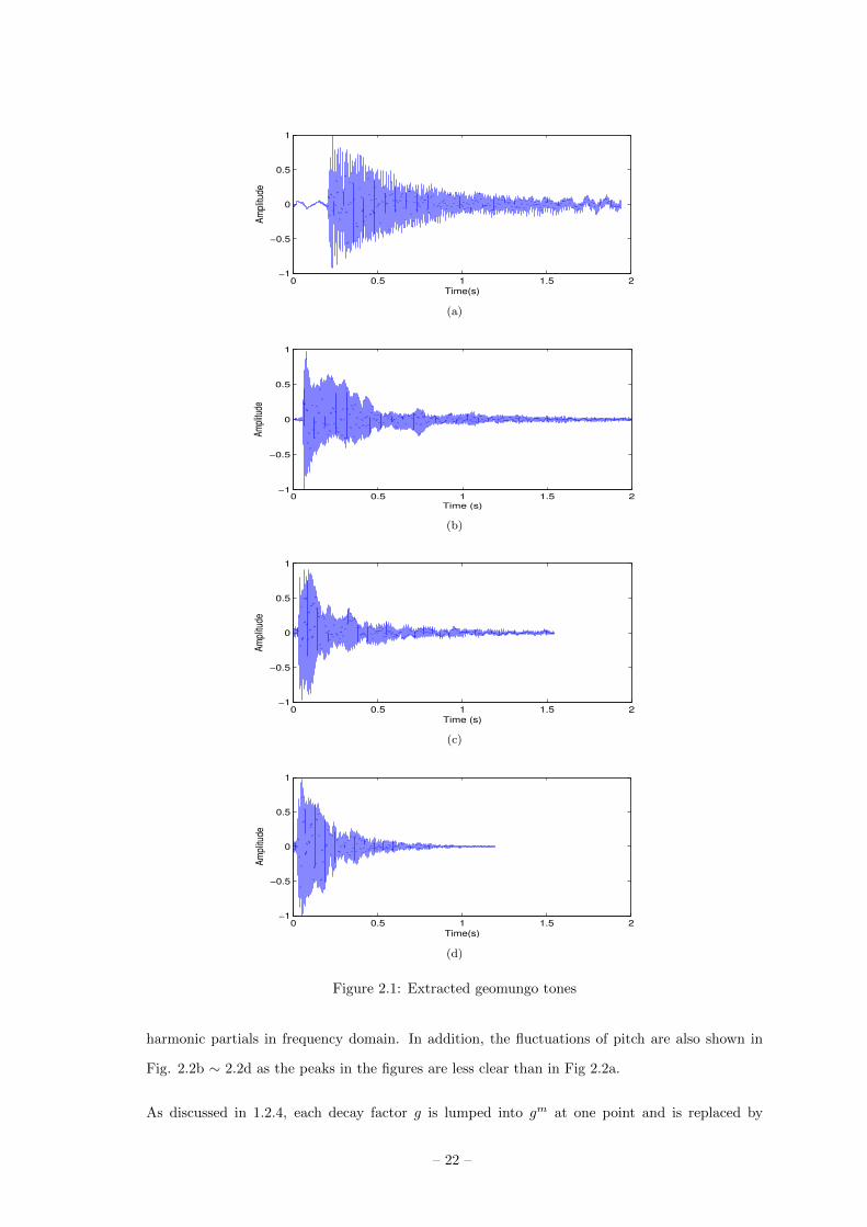
etc. Fig. 2.1 shows four examples of geomungo tones.

Tone of Fig. 2.1a makes a sound of a typical plucked string instrument like guitar. A big difference

between Fig. 2.1a and Fig. 2.1b ∼ 2.1d is that fluctuations of pitch are very great in the latter

(more than 20Hz). Without listening to the tones, the difference can be easily found in the figures

because the amplitude of an ideal tone of a plucked string instrument decreases exponentially.

Fig 2.1a exemplifies the characteristic well, whereas amplitudes decrease irregularly in Fig 2.1b

∼ 2.1d. Thus, I need to consider these acoustical characteristics of the geomungo in the sound

synthesis model.

2.2 Frequency response

Analysis of the signals in frequency domain is required to design a loop filter. At first, I measured

the magnitude spectrums of the extracted geomungo tones by the discrete Fourier transform (DFT)

[53], which is defined by

Xk =

N−1∑n=0

x(tn)e−jwktn , k = 0, 1, 2, ..., N − 1.

Fig. 2.2 shows the results of the transform computed with the fast Fourier transform (FFT)

algorithm of the tones of Fig. 2.1. From the figures, I could roughly find the distribution of

– 21 –

0 0.5 1 1.5 2−1

−0.5

0

0.5

1

Time(s)

Am

plitu

de

(a)

0 0.5 1 1.5 2−1

−0.5

0

0.5

1

Time (s)

Am

plitu

de

(b)

0 0.5 1 1.5 2−1

−0.5

0

0.5

1

Time (s)

Am

plitu

de

(c)

0 0.5 1 1.5 2−1

−0.5

0

0.5

1

Am

plitu

de

Time(s)

(d)

Figure 2.1: Extracted geomungo tones

harmonic partials in frequency domain. In addition, the fluctuations of pitch are also shown in

Fig. 2.2b ∼ 2.2d as the peaks in the figures are less clear than in Fig 2.2a.

As discussed in 1.2.4, each decay factor g is lumped into gm at one point and is replaced by

– 22 –

a filter G(w). Thus, I need to design the filter by estimating the damping factors which mean

the transition of the magnitude at harmonic frequencies of sound signals. The estimation can be

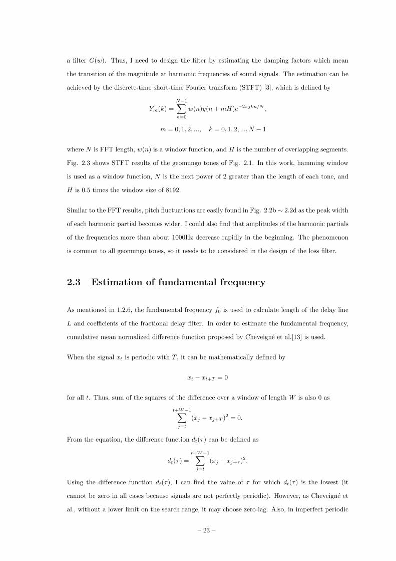
achieved by the discrete-time short-time Fourier transform (STFT) [3], which is defined by

Ym(k) =

N−1∑n=0

w(n)y(n+mH)e−2πjkn/N ,

m = 0, 1, 2, ..., k = 0, 1, 2, ..., N − 1

where N is FFT length, w(n) is a window function, and H is the number of overlapping segments.

Fig. 2.3 shows STFT results of the geomungo tones of Fig. 2.1. In this work, hamming window

is used as a window function, N is the next power of 2 greater than the length of each tone, and

H is 0.5 times the window size of 8192.

Similar to the FFT results, pitch fluctuations are easily found in Fig. 2.2b ∼ 2.2d as the peak width

of each harmonic partial becomes wider. I could also find that amplitudes of the harmonic partials

of the frequencies more than about 1000Hz decrease rapidly in the beginning. The phenomenon

is common to all geomungo tones, so it needs to be considered in the design of the loss filter.

2.3 Estimation of fundamental frequency

As mentioned in 1.2.6, the fundamental frequency f0 is used to calculate length of the delay line

L and coefficients of the fractional delay filter. In order to estimate the fundamental frequency,

cumulative mean normalized difference function proposed by Cheveigne et al.[13] is used.

When the signal xt is periodic with T , it can be mathematically defined by

xt − xt+T = 0

for all t. Thus, sum of the squares of the difference over a window of length W is also 0 as

t+W−1∑j=t

(xj − xj+T )2 = 0.

From the equation, the difference function dt(τ) can be defined as

dt(τ) =

t+W−1∑j=t

(xj − xj+τ )2.

Using the difference function dt(τ), I can find the value of τ for which dt(τ) is the lowest (it

cannot be zero in all cases because signals are not perfectly periodic). However, as Cheveigne et

al., without a lower limit on the search range, it may choose zero-lag. Also, in imperfect periodic

– 23 –

cases, it can choose low lag instead of desired lag. Thus, they proposed an alternative called

cumulative mean normalized difference function:

d′t(τ) = {1, if τ = 0

dt(τ)/[(1/τ)∑τj=1 dt(j)] otherwise.

It avoids selection of zero-lag and low lags by defining the value of the function as 1 at zero-lag.

Thus, it reduces error rate and removes the necessity of upper limit because d′t(τ) remains below

1. The fundamental frequency at τ is estimated as

f0(τ) = fs/d′t(τ).

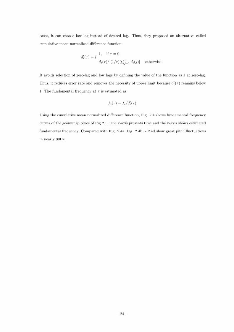
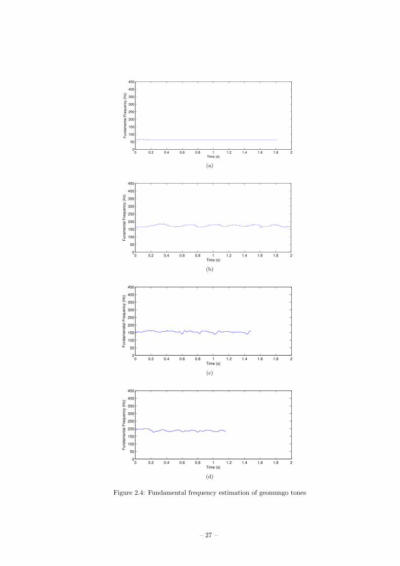
Using the cumulative mean normalized difference function, Fig. 2.4 shows fundamental frequency

curves of the geomungo tones of Fig 2.1. The x-axis presents time and the y-axis shows estimated

fundamental frequency. Compared with Fig. 2.4a, Fig. 2.4b ∼ 2.4d show great pitch fluctuations

in nearly 30Hz.

– 24 –

0 1000 2000 3000 4000 5000−120

−100

−80

−60

−40

−20

Frequency (Hz)

Magnitu

de(d

B)

(a)

0 1000 2000 3000 4000 5000−120

−100

−80

−60

−40

−20

Frequency (Hz)

Mag

nitu

de(d

B)

(b)

0 1000 2000 3000 4000 5000−120

−100

−80

−60

−40

−20

Frequency (Hz)

Mag

nitu

de(d

B)

(c)

0 1000 2000 3000 4000 5000−120

−100

−80

−60

−40

−20

Frequency (Hz)

Magnitu

de(d

B)

(d)

Figure 2.2: Frequency response of geomungo tones

– 25 –

(a)

(b)

(c)

(d)

Figure 2.3: STFT(short-time fourier transform) analysis of geomungo tones

– 26 –

0 0.2 0.4 0.6 0.8 1 1.2 1.4 1.6 1.8 20

50

100

150

200

250

300

350

400

450

Time (s)

Fu

nd

am

en

tal F

req

ue

ncy (

Hz)

(a)

0 0.2 0.4 0.6 0.8 1 1.2 1.4 1.6 1.8 20

50

100

150

200

250

300

350

400

450

Time (s)

Fu

na

me

nta

l F

req

ue

ncy (

Hz)

(b)

0 0.2 0.4 0.6 0.8 1 1.2 1.4 1.6 1.8 20

50

100

150

200

250

300

350

400

450

Time (s)

Fu

nd

am

en

ata

l F

req

ue

ncy (

Hz)

(c)

0 0.2 0.4 0.6 0.8 1 1.2 1.4 1.6 1.8 20

50

100

150

200

250

300

350

400

450

Time (s)

Fu

nd

am

en

tal F

req

ue

ncy (

Hz)

(d)

Figure 2.4: Fundamental frequency estimation of geomungo tones

– 27 –

Chapter 3. General sound synthesis model

3.1 Synthesis model

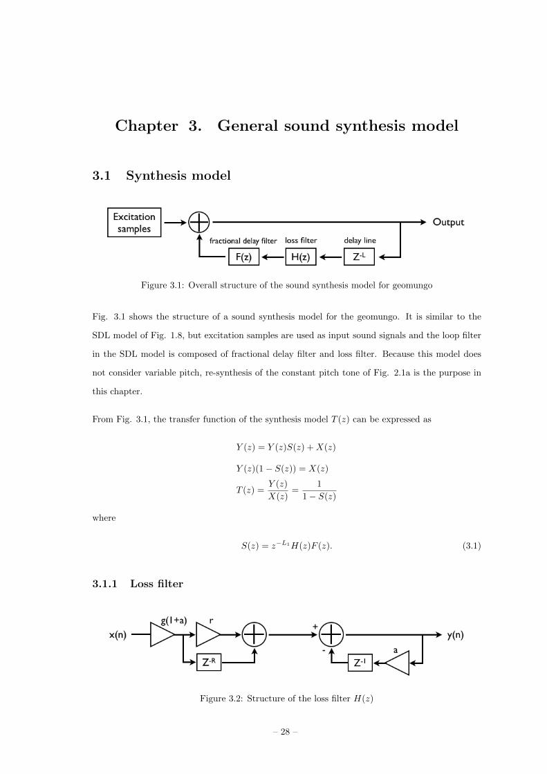
Figure 3.1: Overall structure of the sound synthesis model for geomungo

Fig. 3.1 shows the structure of a sound synthesis model for the geomungo. It is similar to the

SDL model of Fig. 1.8, but excitation samples are used as input sound signals and the loop filter

in the SDL model is composed of fractional delay filter and loss filter. Because this model does

not consider variable pitch, re-synthesis of the constant pitch tone of Fig. 2.1a is the purpose in

this chapter.

From Fig. 3.1, the transfer function of the synthesis model T (z) can be expressed as

Y (z) = Y (z)S(z) +X(z)

Y (z)(1− S(z)) = X(z)

T (z) =Y (z)

X(z)=

1

1− S(z)

where

S(z) = z−L1H(z)F (z). (3.1)

3.1.1 Loss filter

Figure 3.2: Structure of the loss filter H(z)

– 28 –

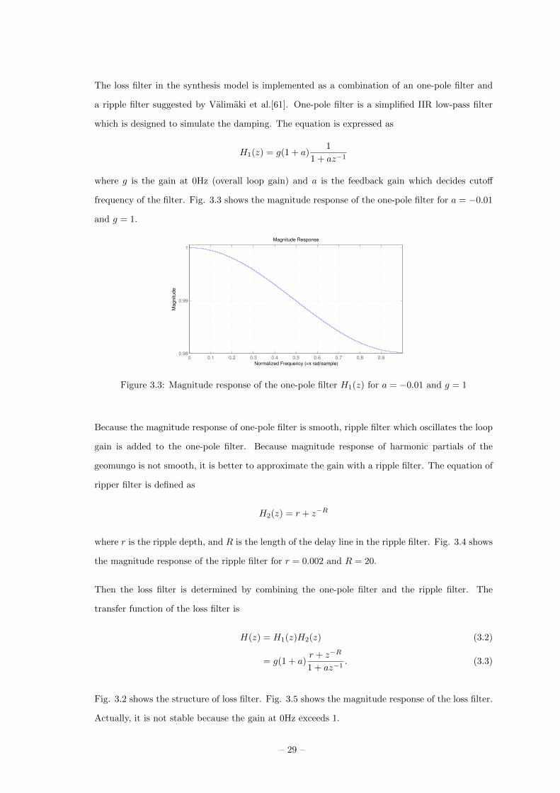
The loss filter in the synthesis model is implemented as a combination of an one-pole filter and

a ripple filter suggested by Valimaki et al.[61]. One-pole filter is a simplified IIR low-pass filter

which is designed to simulate the damping. The equation is expressed as

H1(z) = g(1 + a)1

1 + az−1

where g is the gain at 0Hz (overall loop gain) and a is the feedback gain which decides cutoff

frequency of the filter. Fig. 3.3 shows the magnitude response of the one-pole filter for a = −0.01

and g = 1.

0 0.1 0.2 0.3 0.4 0.5 0.6 0.7 0.8 0.90.98

0.99

1


Ma

gn

itu

de

Magnitude Response

Figure 3.3: Magnitude response of the one-pole filter H1(z) for a = −0.01 and g = 1

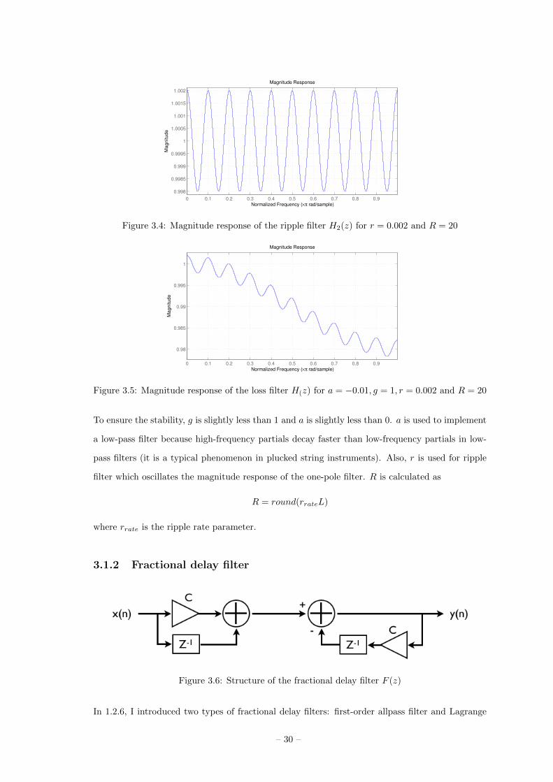
Because the magnitude response of one-pole filter is smooth, ripple filter which oscillates the loop

gain is added to the one-pole filter. Because magnitude response of harmonic partials of the

geomungo is not smooth, it is better to approximate the gain with a ripple filter. The equation of

ripper filter is defined as

H2(z) = r + z−R

where r is the ripple depth, and R is the length of the delay line in the ripple filter. Fig. 3.4 shows

the magnitude response of the ripple filter for r = 0.002 and R = 20.

Then the loss filter is determined by combining the one-pole filter and the ripple filter. The

transfer function of the loss filter is

H(z) = H1(z)H2(z) (3.2)

= g(1 + a)r + z−R

1 + az−1. (3.3)

Fig. 3.2 shows the structure of loss filter. Fig. 3.5 shows the magnitude response of the loss filter.

Actually, it is not stable because the gain at 0Hz exceeds 1.

– 29 –

0 0.1 0.2 0.3 0.4 0.5 0.6 0.7 0.8 0.9

0.998

0.9985

0.999

0.9995

1

1.0005

1.001

1.0015

1.002


Ma

gn

itu

de

Magnitude Response

Figure 3.4: Magnitude response of the ripple filter H2(z) for r = 0.002 and R = 20

0 0.1 0.2 0.3 0.4 0.5 0.6 0.7 0.8 0.9

0.98

0.985

0.99

0.995

1


Ma

gn

itu

de

Magnitude Response

Figure 3.5: Magnitude response of the loss filter H(z) for a = −0.01, g = 1, r = 0.002 and R = 20

To ensure the stability, g is slightly less than 1 and a is slightly less than 0. a is used to implement

a low-pass filter because high-frequency partials decay faster than low-frequency partials in low-

pass filters (it is a typical phenomenon in plucked string instruments). Also, r is used for ripple

filter which oscillates the magnitude response of the one-pole filter. R is calculated as

R = round(rrateL)

where rrate is the ripple rate parameter.


Figure 3.6: Structure of the fractional delay filter F (z)

In 1.2.6, I introduced two types of fractional delay filters: first-order allpass filter and Lagrange

– 30 –

interpolation FIR filter. In this work, the allpass filter is used as a fractional delay filter because

it has a simple structure to approximate the fractional delay and unity magnitude response for all

frequencies. Fig. 3.6 shows the structure of the fractional delay filter.

3.1.3 Delay line

In the original digital waveguide theory, the length of delay line L is decided as

L = fs/f0.

In the proposed sound synthesis model, I estimate the fundamental frequency f0 and use it instead

of f0 as

L = fs/f0.

Other filters used in the model also have phase delays, so the delay line length L1 can be defined

as

L1 = L− PF − PL = fs/f0 − PF − PL

where PF and PL are the phase delay of the fractional delay filter and the loss filter. In this model,

PF is 1−C1+C and PL is R+ 1, so

L1 = fs/f0 −R− 1− 1− C1 + C

.

3.2 Calibration

In this section, I estimate the parameters and extract an excitation sample for the synthesis

model. Based on the delay line length, frequency-dependent gains at the harmonic frequencies are

estimated, and they are used to approximate the coefficients of the loop filter. Then, input signal

is gathered by the inverse loop filter.

In 2.3, I estimated the fundamental frequency of geomungo tones. I decided 63.1Hz as the funda-

mental frequency of Fig. 2.2a by average. Because fs is 44100Hz in this work, L is 698.89.

3.2.1 Estimation of the frequency-dependent loss

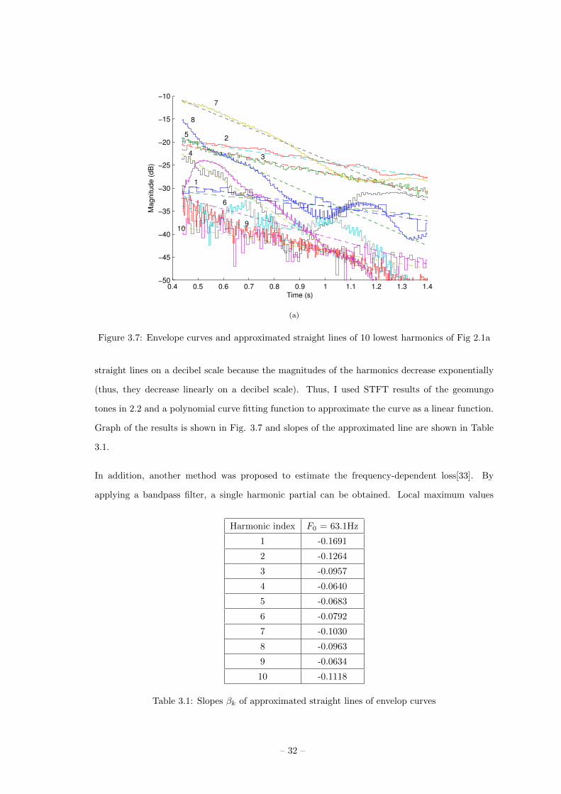
In order to know the loop gains at the harmonic frequencies, the envelope curves meaning the

sequences of magnitude values of the harmonic partials over time need to be approximated as

– 31 –

0.4 0.5 0.6 0.7 0.8 0.9 1 1.1 1.2 1.3 1.4−50

−45

−40

−35

−30

−25

−20

−15

−10

Time (s)

Magnitude (

dB

)

109

6

7

2

3

8

1

4

5

(a)

Figure 3.7: Envelope curves and approximated straight lines of 10 lowest harmonics of Fig 2.1a

straight lines on a decibel scale because the magnitudes of the harmonics decrease exponentially

(thus, they decrease linearly on a decibel scale). Thus, I used STFT results of the geomungo

tones in 2.2 and a polynomial curve fitting function to approximate the curve as a linear function.

Graph of the results is shown in Fig. 3.7 and slopes of the approximated line are shown in Table

3.1.

In addition, another method was proposed to estimate the frequency-dependent loss[33]. By

applying a bandpass filter, a single harmonic partial can be obtained. Local maximum values

Harmonic index F0 = 63.1Hz

1 -0.1691

2 -0.1264

3 -0.0957

4 -0.0640

5 -0.0683

6 -0.0792

7 -0.1030

8 -0.0963

9 -0.0634

10 -0.1118

Table 3.1: Slopes βk of approximated straight lines of envelop curves

– 32 –

are obtained from the bandpassed signal and the amplitude envelope is acquired based on the

values. Because this method was originally proposed for a hybrid waveguide model, so details are

discussed later in the hybrid model chapter. Fig .3.8 compares the losses estimated by the two

methods and it can be found that the results are almost same.

0.4 0.5 0.6 0.7 0.8 0.9 1 1.1 1.2 1.3 1.4−40

−38

−36

−34

−32

−30

−28

Time (s)

Mag

nitu

de (

dB)

0.4 0.5 0.6 0.7 0.8 0.9 1 1.1 1.2 1.3 1.4−35

−30

−25

−20

−15

−10

Time (s)

Magnitu

de (

dB

)

Figure 3.8: Comparison of the estimated losses of the (a) 1st partial and (b) 7th partial. Blue

lines are the losses estimated by STFT, green lines are maximum values of the bandpassed signals,

and red dot lines are approximated straight lines

The loop gains at the harmonic frequencies are calculated by using the slopes of the envelopes as

Gk = 10βkL/20H , k = 1, 2, ..., N

where βk are the slopes of the approximated lines, H is the number of overlapping segments used

in STFT of the geomungo tones, and L is fs/f0. Values of the estimated loop gains are shown in

Table 3.2 and they are used to design the loss filter in next section.

3.2.2 Design of loss filter

In order to design the loss filter of Eq. 3.3, the loop coefficients a and g for the one-pole filter

H1(z) = g(1 + a)/(1+az−1) are estimated first, then r and R for the ripple filter H2(z) = r+z−R

are calculated.

– 33 –

Harmonic index F0 = 63.1Hz

1 0.9901

2 0.9852

3 0.9832

4 0.9856

5 0.9807

6 0.9731

7 0.9594

8 0.9565

9 0.9674

10 0.9373

Table 3.2: Estimated loop gains Gk

One-pole filter design

To design the filter that matches with the desired magnitude at the harmonic frequencies, a high-

order filter instead of an one-pole filter needs to be designed, but it cannot be used in real-time

applications. Thus, I approximated the gains by using the weighted least-squares method in

which the solution minimizes the sum of products of an error weighting function and squares of

the errors (differences between the magnitude responses of the filter and the estimated loop gains).

The equation is shown as

E =

N∑k=1

W (Gk)[|H1(wk)| −Gk]2 (3.4)

where N is the maximum order of harmonics used to design the filter, W (Gk) is an error weighting

function and wk means kth harmonic frequency. In this work, N is 10 and W (Gk) is used as

W (Gk) =1

1−Gk

to provide a larger weight to the harmonics of larger gain.

The coefficient g of the one-pole filter is generally selected as G1 which is the loop gain value at

the fundamental frequency. Then, a is chosen from −1 to 0 which minimizes the error E. Fig.

3.9 shows the value of E on the coefficient a. From the graph, I can find that E is minimized at

a = −0.7453 on Fig. 3.9a.

Ripple filter design

I used the design method of the ripple filter proposed by Valimaki et al.[61]. From the second

partial, the partial that has the largest Gk value is selected and I denote the harmonic index by

– 34 –

−0.85 −0.8 −0.75 −0.7 −0.65 −0.6 −0.55 −0.5 −0.450

0.01

0.02

0.03

0.04

0.05

0.06

0.07

0.08

0.09

0.1

a

Err

or

Figure 3.9: Magnitude of the error E versus the coefficient a

kmax. In this work, kmax = 4 (G4 = 0.9856).

Then the absolute value of r is determined as

|r| = Gkmax− |H1(wkmax

)|

where H1(wkmax) is the value of the one-pole filter H1(z) at the harmonic of kmax (|r| = 0.0025).

The sign of r is determined by comparison of the first partial’s gain and the magnitude of the

one-pole filter at the first harmonic frequency. If the first partial’s gain is bigger, then the sign

of r is positive. Otherwise, the sign of r is negative. Thus, the sign of r is positive in this work

because G1 = 0.9901 > H1(w1) = 0.9896.

When checking a stability, the filter is stable because g + r = 0.9926 < 1. Thus, the sign of r is

positive. If the filter was unstable, the sign of r would be inverted. Fig. 3.10 shows the magnitude

response of the filter and Gk values.

Finally, in order to set the value of R, the ripple rate parameter rrate is determined as 1/kmax for

positive r and 1/(2kmax) for negative r. Thus, in this work, rrate is 1/4 because r is 0.0025.

3.2.3 Design of allpass filter and delay line

Because L is 698.89, the fractional delay is 0.89 and the length of the delay line is 698. The value

C in the allpass filter of in Eq. 1.7 is decided as

– 35 –

0 100 200 300 400 500 600 7000.9

0.91

0.92

0.93

0.94

0.95

0.96

0.97

0.98

0.99

1

Frequency (Hz)

Ma

gn

itu

de

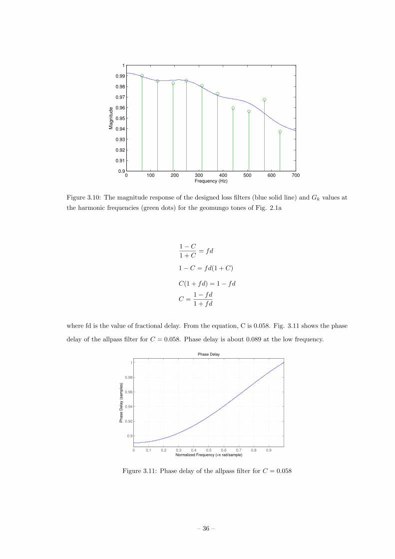
Figure 3.10: The magnitude response of the designed loss filters (blue solid line) and Gk values at

the harmonic frequencies (green dots) for the geomungo tones of Fig. 2.1a

1− C1 + C

= fd

1− C = fd(1 + C)

C(1 + fd) = 1− fd

C =1− fd1 + fd

where fd is the value of fractional delay. From the equation, C is 0.058. Fig. 3.11 shows the phase

delay of the allpass filter for C = 0.058. Phase delay is about 0.089 at the low frequency.

0 0.1 0.2 0.3 0.4 0.5 0.6 0.7 0.8 0.9

0.9

0.92

0.94

0.96

0.98

1


Ph

ase

De

lay (

sa

mp

les)

Phase Delay

Figure 3.11: Phase delay of the allpass filter for C = 0.058

– 36 –

3.2.4 Inverse filtering

As discussed in 1.2.5, an excitation sample which is used as an input signal in the synthesis model

can be extracted by applying inverse filtering to the extracted geomungo tone. Thus, this section

starts with implementation of the inverse filter of the string model S(z) in Eq.3.1 as

S−1(z) = 1− z−L1F (z)H(z)

= 1− z−L1 ∗ c+ z−1

1 + cz−1∗ g(1 + a)

r + z−R

1 + az−1

=A(z)

B(z)

where

A(z) = 1 + (c+ a)z−1 + acz−2 − g(1 + a)crz−L1 − g(1 + a)rz−(L1+1)

− g(1 + a)cz−(L1+R) − g(1 + a)z−(L1+1+R)

B(z) = 1 + (c+ a)z−1 + acz−2.

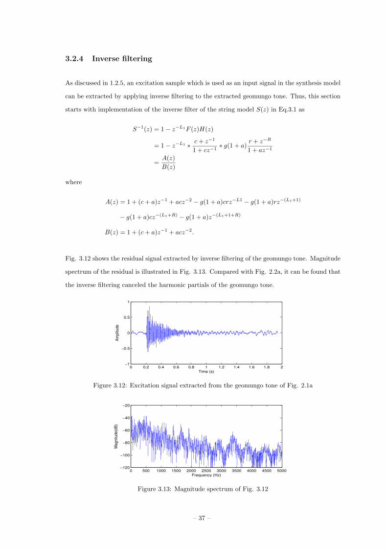
Fig. 3.12 shows the residual signal extracted by inverse filtering of the geomungo tone. Magnitude

spectrum of the residual is illustrated in Fig. 3.13. Compared with Fig. 2.2a, it can be found that

the inverse filtering canceled the harmonic partials of the geomungo tone.

0 0.2 0.4 0.6 0.8 1 1.2 1.4 1.6 1.8 2−1

−0.5

0

0.5

1

Time (s)

Am

plit

ud

e

Figure 3.12: Excitation signal extracted from the geomungo tone of Fig. 2.1a

0 500 1000 1500 2000 2500 3000 3500 4000 4500 5000−120

−100

−80

−60

−40

−20

Frequency (Hz)

Ma

gn

itud

e(d

B)

Figure 3.13: Magnitude spectrum of Fig. 3.12

– 37 –

3.3 Synthesis

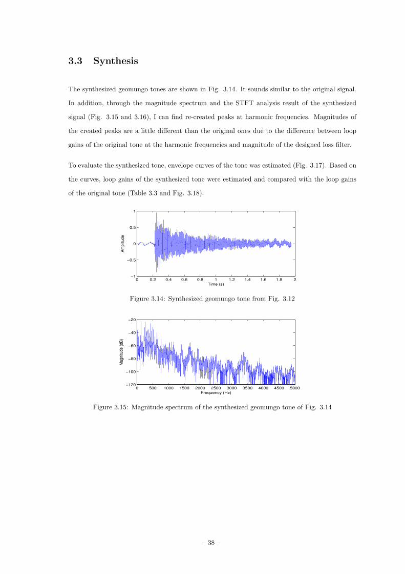
The synthesized geomungo tones are shown in Fig. 3.14. It sounds similar to the original signal.

In addition, through the magnitude spectrum and the STFT analysis result of the synthesized

signal (Fig. 3.15 and 3.16), I can find re-created peaks at harmonic frequencies. Magnitudes of

the created peaks are a little different than the original ones due to the difference between loop

gains of the original tone at the harmonic frequencies and magnitude of the designed loss filter.

To evaluate the synthesized tone, envelope curves of the tone was estimated (Fig. 3.17). Based on

the curves, loop gains of the synthesized tone were estimated and compared with the loop gains

of the original tone (Table 3.3 and Fig. 3.18).

0 0.2 0.4 0.6 0.8 1 1.2 1.4 1.6 1.8 2−1

−0.5

0

0.5

1

Time (s)

Am

plit

ud

e

Figure 3.14: Synthesized geomungo tone from Fig. 3.12

0 500 1000 1500 2000 2500 3000 3500 4000 4500 5000−120

−100

−80

−60

−40

−20

Frequency (Hz)

Ma

gn

itud

e (

dB

)

Figure 3.15: Magnitude spectrum of the synthesized geomungo tone of Fig. 3.14

– 38 –

Figure 3.16: STFT analysis of the synthesized geomungo tone of Fig. 3.14

0.4 0.5 0.6 0.7 0.8 0.9 1 1.1 1.2 1.3 1.4−50

−45

−40

−35

−30

−25

−20

−15

−10

Figure 3.17: Envelope curves of the synthesized tone of Fig. 3.14

– 39 –

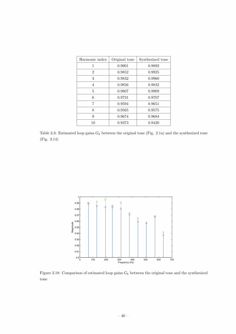
Harmonic index Original tone Synthesized tone

1 0.9901 0.9892

2 0.9852 0.9925

3 0.9832 0.9960

4 0.9856 0.9832

5 0.9807 0.9909

6 0.9731 0.9707

7 0.9594 0.9651

8 0.9565 0.9575

9 0.9674 0.9684

10 0.9373 0.9420

Table 3.3: Estimated loop gains Gk between the original tone (Fig. 2.1a) and the synthesized tone

(Fig. 3.14)

0 100 200 300 400 500 600 7000.9

0.91

0.92

0.93

0.94

0.95

0.96

0.97

0.98

0.99

1

Frequency (Hz)

Ma

gn

itu

de

Figure 3.18: Comparison of estimated loop gains Gk between the original tone and the synthesized

tone

– 40 –

Chapter 4. Time-varying synthesis model

4.1 Synthesis model

The synthesis model discussed in chapter 3.1 works well enough to re-synthesize the sounds of the

recorded geomungo tones. However, it needs to be improved to synthesize the tones of fluctuating

pitches. Thus, in this section, I propose a revised model to synthesize the geomungo tones more

naturally.

The previous model cannot reflect pitch variation because the length of the delay line was fixed

in the previous model. However, as discussed in 2.3, the geomungo tones have a great pitch

fluctuations. Since a geomungo technique called Nonghyun (similar to vibrato and trill, but more

dynamic) occurs the phenomenon, the pitch fluctuation is distinguished from pitch glide (pitch

variation) meaning that the fundamental frequency of the instrument decreases after plucking due

to the transverse vibration[32]. It is rather more similar to the glissando effect for the fretless

instrument discussed in [15].

Figure 4.1: Overall structure of the revised sound model

Fig. 4.1 shows the revised model to reflect the fluctuating pitch. All filters used in this model are

time-varying filters to synthesize variable pitch sounds. The fractional delay filter is changed to

the Lagrange interpolation FIR filter discussed in 1.2.6 because it is more favorable for variable

delay. Length of the delay line is changed to be time-varying. Also, a gain factor gc is added to

the synthesis model to preserve the energy when the pitch is altered [40]. The equation of the gc

– 41 –

is expressed as

gc =√

1−∆x

≈ 1− ∆x

2for small x

(∆x = xn − xn−1)

where xn is the position in the string at time index n and ∆x is the change of the delay line length.

4.1.1 Loss filter

Figure 4.2: Structure of the time-varying loss filter H(z)

Fig. 4.2 shows the structure of the time-varying loss filter. A ripple filter used in the previous

loss filter model is removed in this model because it decreases the sound quality of the synthesis

model when changing the filter coefficients. Also, the coefficients in the filter need to be changed

as time dependent values because amplitudes of the variable pitch sounds such as Fig. 2.1b and

2.1d do not decrease exponentially as discussed in 2.1. There are two coefficients in this filter: the

loop gain g and the feedback gain a. However, changing the feedback gain results in transients

effects which create audible clicks [16]. Thus, the loop gain coefficient g is changed to depend on

time as g(n) and a transfer function of the time-varying loss filter is expressed as

H(z) = gn(1 + a)1

1 + az−1.


As discussed in 1.2.6, Lagrange interpolation FIR filter is better for variable delay line. Because the

frequency changes over time, the desired fractional delay factor D is changed as a time-dependent

value D(n) as

D(n) =fs

f0(n)− floor[ fs

f0(n)].

Therefore, the fractional delay filter coefficients are altered as h0(n), h1(n), h2(n), and h3(n) (Fig.

4.3).

– 42 –

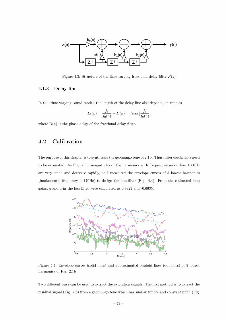
Figure 4.3: Structure of the time-varying fractional delay filter F (z)

4.1.3 Delay line

In this time-varying sound model, the length of the delay line also depends on time as

L1(n) =fs

f0(n)−D(n) = floor[

fsf0(n)

]

where D(n) is the phase delay of the fractional delay filter.

4.2 Calibration

The purpose of this chapter is to synthesize the geomungo tone of 2.1b. Thus, filter coefficients need

to be estimated. As Fig. 2.3b, magnitudes of the harmonics with frequencies more than 1000Hz

are very small and decrease rapidly, so I measured the envelope curves of 5 lowest harmonics

(fundamental frequency is 170Hz) to design the loss filter (Fig. 4.4). From the estimated loop

gains, g and a in the loss filter were calculated as 0.9923 and -0.6635.

0.6 0.8 1 1.2 1.4 1.6 1.8−80

−70

−60

−50

−40

−30

−20

Time (s)

Ma

gn

itu

de

(d

B)

Figure 4.4: Envelope curves (solid lines) and approximated straight lines (dot lines) of 5 lowest

harmonics of Fig. 2.1b

Two different ways can be used to extract the excitation signals. The first method is to extract the

residual signal (Fig. 4.6) from a geomungo tone which has similar timbre and constant pitch (Fig.

– 43 –

4.5). The second method is to use the target signal itself. Since the frequency of the inverse filter

does not depend on time but the frequency of the geomungo tone varies depending on time, the

vibrating sound after the plucking sound cannot be inverse filtered. Thus, length of the residual

signal should be shorted by deamplifyng and removing the vibrating sound after the plucking

sound. Fig. 4.7 shows the residual signal generated by the second method.

Calibration method used in this section is same as 3.2. Because magnitudes of the harmonics with

frequencies more than 1000Hz are also very small, loop gains of 5 lowest harmonics were estimated

for inverse filtering.

0 0.5 1 1.5 2−1

−0.5

0

0.5

1

Time (s)

Am

plitu

de

Figure 4.5: A geomungo tone having constant pitch for generating an excitation signal

0 0.5 1 1.5 2−1

−0.5

0

0.5

1

Time (s)

Am

plitu

de

Figure 4.6: Excitation signal extracted from the geomungo tone of Fig. 4.5

0 0.5 1 1.5 2−1

−0.5

0

0.5

1

Time (s)

Am

plitu

de

Figure 4.7: Excitation signal extracted from the geomungo tone of Fig. 2.1b

– 44 –

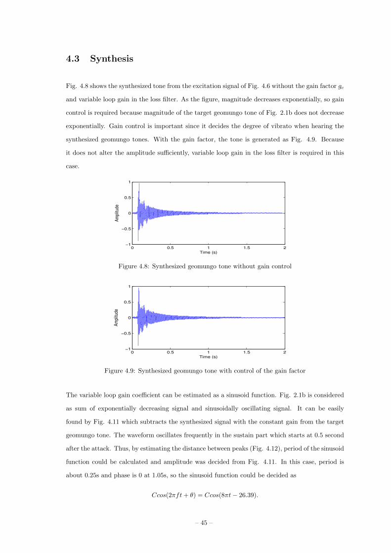
4.3 Synthesis

Fig. 4.8 shows the synthesized tone from the excitation signal of Fig. 4.6 without the gain factor gc

and variable loop gain in the loss filter. As the figure, magnitude decreases exponentially, so gain

control is required because magnitude of the target geomungo tone of Fig. 2.1b does not decrease

exponentially. Gain control is important since it decides the degree of vibrato when hearing the

synthesized geomungo tones. With the gain factor, the tone is generated as Fig. 4.9. Because

it does not alter the amplitude sufficiently, variable loop gain in the loss filter is required in this

case.

0 0.5 1 1.5 2−1

−0.5

0

0.5

1

Time (s)

Am

plitu

de

Figure 4.8: Synthesized geomungo tone without gain control

0 0.5 1 1.5 2−1

−0.5

0

0.5

1

Time (s)

Am

plitu

de

Figure 4.9: Synthesized geomungo tone with control of the gain factor

The variable loop gain coefficient can be estimated as a sinusoid function. Fig. 2.1b is considered

as sum of exponentially decreasing signal and sinusoidally oscillating signal. It can be easily

found by Fig. 4.11 which subtracts the synthesized signal with the constant gain from the target

geomungo tone. The waveform oscillates frequently in the sustain part which starts at 0.5 second

after the attack. Thus, by estimating the distance between peaks (Fig. 4.12), period of the sinusoid

function could be calculated and amplitude was decided from Fig. 4.11. In this case, period is

about 0.25s and phase is 0 at 1.05s, so the sinusoid function could be decided as

Ccos(2πft+ θ) = Ccos(8πt− 26.39).

– 45 –

Because the loop gain gn means the decay rate of the synthesized signal, so differentiation of the

sinusoid function was added to the constant loop gain value to define gn as

gn = g − C ′sin(8πt− 26.39).

where g means the constant loop gain value estimated by inverse filtering and C is used as 0.05 in

this case. Fig. 4.13 shows the calculated loop gain coefficient.

The variable loop gain coefficient can also be compared with the envelop curve. Fig. 4.10 shows

the envelope curves of the synthesized tone without gain control, and the curves do not fluctuate

enough to hear the vibrato. However, in Fig. 4.4, it can be found that the red solid curve, the

envelop curve of the second lowest harmonic, oscillates about 10dB while decaying. Positions of

the curve are almost consistent with the positions of the peaks chosen in Fig. 4.12 (1.05 and 1.3

second).

0.6 0.8 1 1.2 1.4 1.6 1.8−80

−70

−60

−50

−40

−30

−20

Time (s)

Ma

gn

itu

de

(d

B)

Figure 4.10: Envelope curves of the synthesized geomungo tone without gain control

0 0.5 1 1.5 2−1

−0.5

0

0.5

1

Time (s)

Am

plitu

de

Figure 4.11: Magnitude difference between the target signal and Fig 4.9

The sinusoid function for the variable loop gain coefficient is also consistent with the loop gain

curve at the second lowest harmonic frequency after 0.5 second (Fig. 4.14), which is calculated

based on a series of the slopes of the lines approximated in a narrow range of the envelope curve.

– 46 –

0 0.5 1 1.5 2−1

−0.5

0

0.5

1

Time (s)

Am

plitu

de

1.301.050.25

Figure 4.12: Estimate of the distance between peaks in Fig 4.11

It may use the loop gain curve itself as a variable loop gain coefficient, but it makes the filter

unstable and amplitude of the generated signal exceeds unity and the envelop curves of other

harmonic frequencies do not fluctuate significantly (the loop gain value decides the decay rates of

all harmonic partials). It means that frequency of the approximated sinusoidal function should be

similar to the loop gain of the second lowest harmonic, but amplitude of the function should be

smaller.

0 0.5 1 1.5 20.9

0.95

1

1.05

1.1

Time (s)

g

Figure 4.13: Variable loop gain coefficient gn used for the time-varying loss filter

0 0.5 1 1.5 20.8

0.85

0.9

0.95

1

1.05

1.1

1.15

Time (s)

g

Figure 4.14: Comparison of the variable loop gain coefficient with the estimated loop gain of the

second lowest harmonic

The fundamental frequency curve measured in 2.3 also needs to be modified for controlling the

length of delay line and the fractional delay filter because there was a slight difference in the

fundamental frequency of the synthesized tone. The modification is applied a little differently for

– 47 –

each sound, but the frequency curve was pushed back by 1000 samples and increased by 5Hz in

this case. Finally, the waveform of the re-synthesized geomungo tone of Fig. 2.1b from Fig. 4.5 is

shown in Fig. 4.15. Also, Fig. 4.16 shows the synthesized geomungo tone from Fig. 4.7.

0 0.5 1 1.5 2−1

−0.5

0

0.5

1

Time (s)

Am

plitu

de

Figure 4.15: Synthesized geomungo tone from the residual signal of Fig. 4.6

0 0.5 1 1.5 2−1

−0.5

0

0.5

1

Time (s)

Am

plitu

de

Figure 4.16: Synthesized geomungo tone from the residual signal of Fig. 4.7

Envelope curves of Fig. 4.15 is shown in Fig. 4.17. Compared with the envelope curves of the

original geomungo tone (Fig. 4.4), the blue curve, the envelope curve of the first lowest harmonic,

oscillates significantly while decaying instead of the red curve, the second lowest harmonic. The

difference shows the limitation of the digital waveguide modeling that each harmonic cannot be

controlled separately because harmonics are created using a digital delay line.

0.6 0.8 1 1.2 1.4 1.6 1.8−80

−70

−60

−50

−40

−30

−20

Time (s)

Magnitu

de (

dB

)

Figure 4.17: Envelope curves of the synthesized geomungo tone of Fig. 4.15

– 48 –

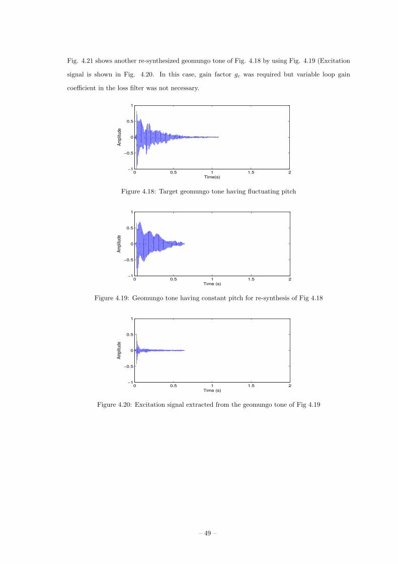
Fig. 4.21 shows another re-synthesized geomungo tone of Fig. 4.18 by using Fig. 4.19 (Excitation

signal is shown in Fig. 4.20. In this case, gain factor gc was required but variable loop gain

coefficient in the loss filter was not necessary.

0 0.5 1 1.5 2−1

−0.5

0

0.5

1

Am

plitu

de

Time(s)

Figure 4.18: Target geomungo tone having fluctuating pitch

0 0.5 1 1.5 2−1

−0.5

0

0.5

1

Time (s)

Am

plitu

de

Figure 4.19: Geomungo tone having constant pitch for re-synthesis of Fig 4.18

0 0.5 1 1.5 2−1

−0.5

0

0.5

1

Time (s)

Am

plitu

de

Figure 4.20: Excitation signal extracted from the geomungo tone of Fig 4.19

– 49 –

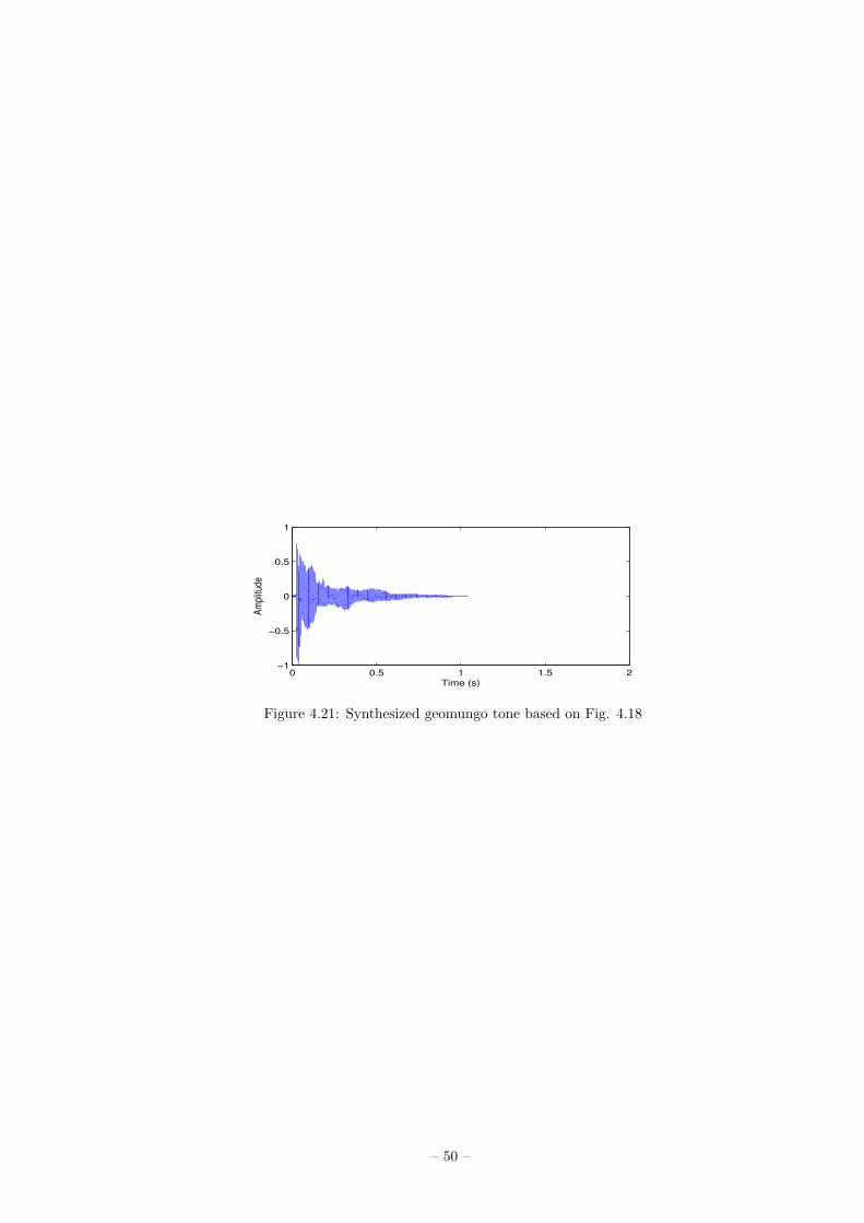
0 0.5 1 1.5 2−1

−0.5

0

0.5

1

Time (s)

Am

plitu

de

Figure 4.21: Synthesized geomungo tone based on Fig. 4.18

– 50 –

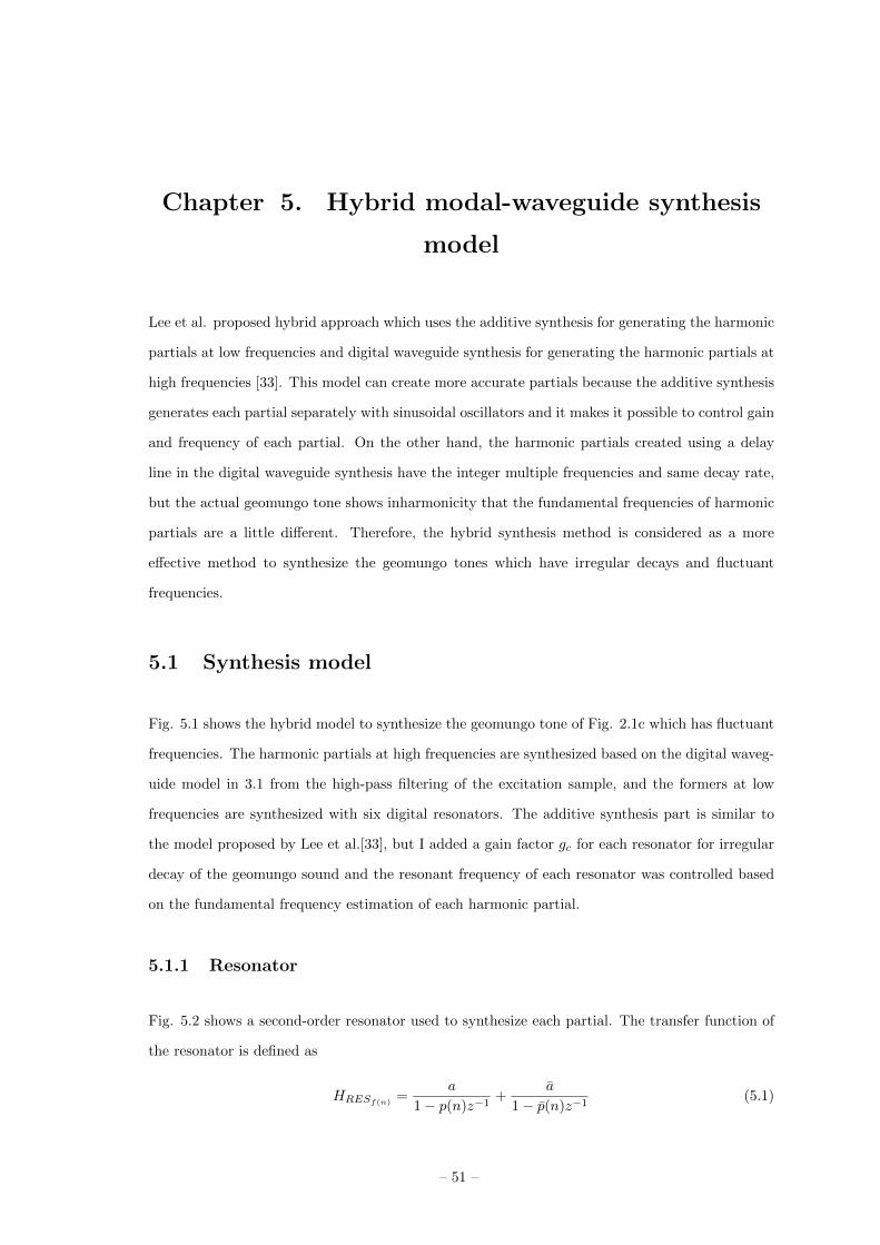
Chapter 5. Hybrid modal-waveguide synthesis

model

Lee et al. proposed hybrid approach which uses the additive synthesis for generating the harmonic

partials at low frequencies and digital waveguide synthesis for generating the harmonic partials at

high frequencies [33]. This model can create more accurate partials because the additive synthesis

generates each partial separately with sinusoidal oscillators and it makes it possible to control gain

and frequency of each partial. On the other hand, the harmonic partials created using a delay

line in the digital waveguide synthesis have the integer multiple frequencies and same decay rate,

but the actual geomungo tone shows inharmonicity that the fundamental frequencies of harmonic

partials are a little different. Therefore, the hybrid synthesis method is considered as a more

effective method to synthesize the geomungo tones which have irregular decays and fluctuant

frequencies.

5.1 Synthesis model

Fig. 5.1 shows the hybrid model to synthesize the geomungo tone of Fig. 2.1c which has fluctuant

frequencies. The harmonic partials at high frequencies are synthesized based on the digital waveg-

uide model in 3.1 from the high-pass filtering of the excitation sample, and the formers at low

frequencies are synthesized with six digital resonators. The additive synthesis part is similar to

the model proposed by Lee et al.[33], but I added a gain factor gc for each resonator for irregular

decay of the geomungo sound and the resonant frequency of each resonator was controlled based

on the fundamental frequency estimation of each harmonic partial.

5.1.1 Resonator

Fig. 5.2 shows a second-order resonator used to synthesize each partial. The transfer function of

the resonator is defined as

HRESf(n)=

a

1− p(n)z−1+

a

1− p(n)z−1(5.1)

– 51 –

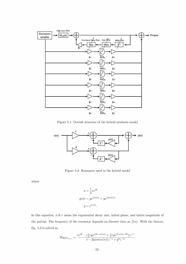
Figure 5.1: Overall structure of the hybrid synthesis model

Figure 5.2: Resonator used in the hybrid model

where

a =1

2rejθ

p(n) = gejw(n) = gej2πf(n)

g = eσ/fs .

In this equation, σ, θ, r mean the exponential decay rate, initial phase, and initial magnitude of

the partial. The frequency of the resonator depends on discrete time as f(n). With the factors,

Eq. 5.2 is solved as

HRESf(n)=rejθ − ( 1

2rgej(θ−w(n)) + 1

2rgej(w(n)−θ))z−1

1− 2gcos(w(n))z−1 + g2z−2.

– 52 –

Fig. 5.3 shows a signal generated by the resonator. A clear peak at 200Hz can be found in the

magnitude response (Fig. 5.4).

0 0.2 0.4 0.6 0.8 1−1

−0.5

0

0.5

1

Time (s)

Am

plit

ude

Figure 5.3: Waveform of a signal generated by the resonator when the initial magnitude r = 1,

initial phase θ = 0, exponential decay rate g = 0.9999, and frequency is 200Hz

0 100 200 300 400 500−60

−50

−40

−30

−20

−10

0

Frequency (Hz)

Magnitude(d

B)

Figure 5.4: Magnitude response of the signal Fig. 5.3

5.2 Calibration

5.2.1 Extraction of harmonic partials

In order to generate harmonic partials, parameters of the resonators are required to be estimated

from the harmonic partials of the geomungo tone of Fig. 2.1c. Each partial can be extracted by a

band-pass filter, which was designed using Kaiser window FIR filter design approach, a technique

to design a multiband FIR filter with cutoff frequencies and ripple parameters[39]. Fig. 5.5 shows

the magnitude response of a bandpass filter to extract the third harmonic partial. Passband exists

around 480Hz, and other stopband regions are attenuated below -100dB. Using the designed

bandpass filter, 6 lowest harmonic partials were extracted as shown in Fig. 5.6. The peaks are

shown in the magnitude spectrums of the partials (Fig. 5.7) and revealed better when compared

– 53 –

the magnitude response of the sum of the extracted partials with the magnitude response of the

geomungo tone (Fig. 5.8).

0 1000 2000 3000 4000 5000

−150

−100

−50

0

Frequency (Hz)

Magnitude (

dB

)


Figure 5.5: Magnitude response of the bandpass filter designed using Kaiser window FIR filter

design approach for the third harmonic partial of the geomungo tone of 2.1c

5.2.2 Estimation of decay rate and initial magnitude

The second method to estimate the decay rates of the harmonic partials discussed in 3.2.1 is

also used to estimate the exponential decay rate and initial magnitude of each partial. In the

waveforms, the positive local maximum points are obtained by taking the positive points of zero

derivative (Fig. 5.9). A straight line can be fitted from the positive local maximum points on a

decibel scale (Fig. 5.10). Then the slope of the fitted line becomes the exponential decay rate, and

the value of the line at t = 0 becomes the initial magnitude. To use the exponential decay rate

for the filter, it needs to be calculated as σ = log(10(fsσ0/20)) when σ0 is the estimated decay rate

because σ0 is defined on time unit and decibel scale, but σ is defined on sample unit and linear

scale. Table 5.1 shows the estimated initial magnitudes and decay rates.

Harmonic index Initial magnitude r Decay rate σ

1 0.0067 -1.4204

2 0.0055 -2.3893

3 0.0058 -3.8327

4 0.0030 -3.4683

5 0.0027 -3.4736

6 0.0026 -12.5970

Table 5.1: Estimated initial magnitudes and decay rates

– 54 –

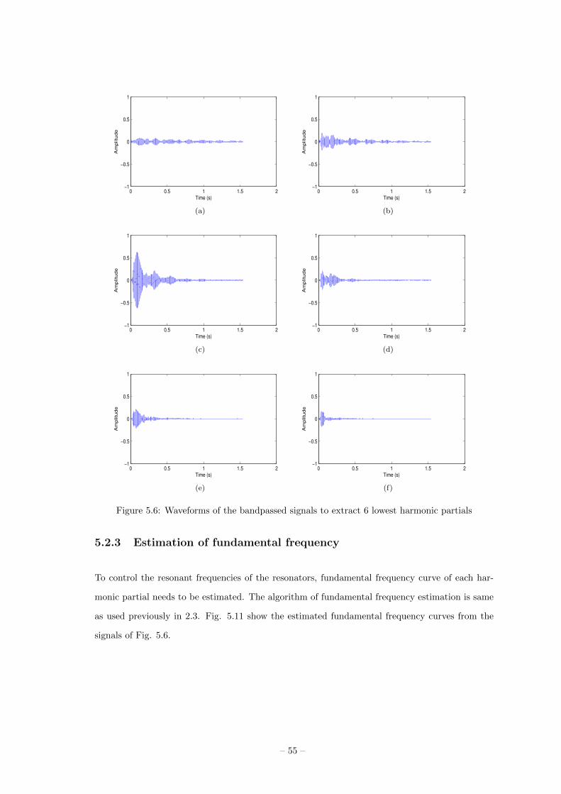
0 0.5 1 1.5 2−1

−0.5

0

0.5

1

Time (s)

Am

plitu

de

(a)

0 0.5 1 1.5 2−1

−0.5

0

0.5

1

Time (s)

Am

plitu

de

(b)

0 0.5 1 1.5 2−1

−0.5

0

0.5

1

Time (s)

Am

plitu

de

(c)

0 0.5 1 1.5 2−1

−0.5

0

0.5

1

Time (s)

Am

plitu

de

(d)

0 0.5 1 1.5 2−1

−0.5

0

0.5

1

Time (s)

Am

plitu

de

(e)

0 0.5 1 1.5 2−1

−0.5

0

0.5

1

Time (s)

Am

plitu

de

(f)

Figure 5.6: Waveforms of the bandpassed signals to extract 6 lowest harmonic partials

5.2.3 Estimation of fundamental frequency

To control the resonant frequencies of the resonators, fundamental frequency curve of each har-

monic partial needs to be estimated. The algorithm of fundamental frequency estimation is same

as used previously in 2.3. Fig. 5.11 show the estimated fundamental frequency curves from the

signals of Fig. 5.6.

– 55 –

0 1000 2000 3000 4000 5000−120

−100

−80

−60

−40

−20

Frequency (Hz)

Magnitude(d

B)

(a)

0 1000 2000 3000 4000 5000−120

−100

−80

−60

−40

−20

Frequency (Hz)

Magnitude(d

B)

(b)

0 1000 2000 3000 4000 5000−120

−100

−80

−60

−40

−20

Frequency (Hz)

Magnitude(d

B)

(c)

0 1000 2000 3000 4000 5000−120

−100

−80

−60

−40

−20

Frequency (Hz)

Magnitude(d

B)

(d)

0 1000 2000 3000 4000 5000−120

−100

−80

−60

−40

−20

Frequency (Hz)

Magnitude(d

B)

(e)

0 1000 2000 3000 4000 5000−120

−100

−80

−60

−40

−20

Frequency (Hz)

Magnitude(d

B)

(f)

Figure 5.7: Magnitude spectrum of the bandpassed signals

5.2.4 Estimation of gain factor

Because the amplitude of each harmonic partial does not decrease exponentially as discussed above,

the gain factor gc should be estimated. The estimation method is similar to the method used in

the time-varying waveguide model to estimate the variable loop gain of the loss filter. Sinusoidal

functions which are used as the gain factors in the hybrid model are fitted with the local maximum

points of the bandpassed signals. Because amplitude of the third harmonic partial is the biggest,

so the periods of the sinusoidal functions of other harmonic partials are based on the period of the

sinusoidal function of the third harmonic partials. The period approximated based on the third

harmonic partial is about 0.22 second, and the formers for other harmonic partials are near 0.11

– 56 –

0 1000 2000 3000 4000 5000−120

−100

−80

−60

−40

−20

Frequency (Hz)

Magnitude(d

B)

Figure 5.8: Comparison of the magnitude spectrums of the sum of the bandpassed signals (green

curve) and the original geomungo tone (blud curve, Fig. 2.2c)

0.2 0.22 0.24 0.26 0.28 0.3−0.2

−0.15

−0.1

−0.05

0

0.05

0.1

0.15

0.2

Time (s)

Am

plit

ude

Figure 5.9: Comparison of the waveform of the bandpassed signal for the third partial (blue curve)

and the positive local maximum points (green curve)

0 0.5 1 1.5−80

−70

−60

−50

−40

−30

−20

−10

0

Time (s)

Magnitude (

dB

)

Figure 5.10: Approximated straight line (green curve) is fitted over the positive local maximum

points (blue curve)

second. Fig. 5.13 shows the synthesized signal for the resynthesis of the third partial (Fig. 5.12)

without the gain factor. With the gain factor of a sinusoidal function, waveform of the synthesized

signal (Fig. 5.14 is more similar to the target signal.

– 57 –

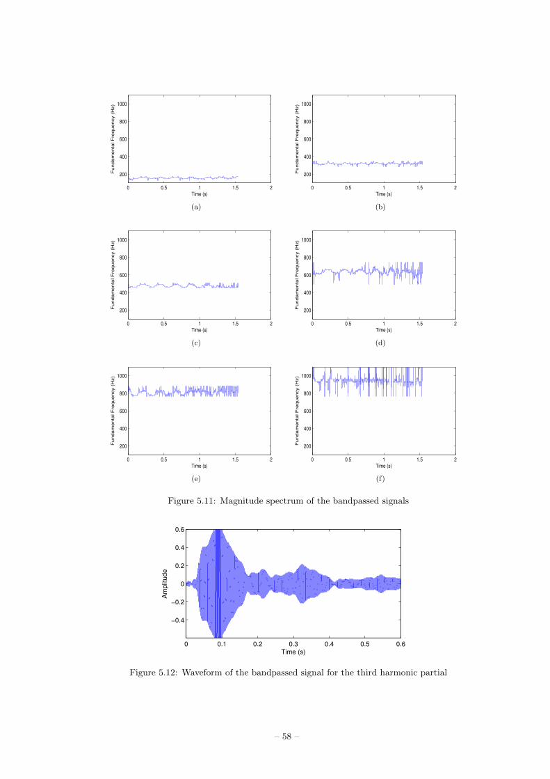
0 0.5 1 1.5 2

200

400

600

800

1000

Time (s)

Fundam

enta

l F

requency (

Hz)

(a)

0 0.5 1 1.5 2

200

400

600

800

1000

Time (s)

Fundam

enta

l F

requency (

Hz)

(b)

0 0.5 1 1.5 2

200

400

600

800

1000

Time (s)

Fundam

enta

l F

requency (

Hz)

(c)

0 0.5 1 1.5 2

200

400

600

800

1000

Time (s)

Fundam

enta

l F

requency (

Hz)

(d)

0 0.5 1 1.5 2

200

400

600

800

1000

Time (s)

Fundam

enta

l F

requency (

Hz)

(e)

0 0.5 1 1.5 2

200

400

600

800

1000

Time (s)

Fundam

enta

l F

requency (

Hz)

(f)

Figure 5.11: Magnitude spectrum of the bandpassed signals

0 0.1 0.2 0.3 0.4 0.5 0.6

−0.4

−0.2

0

0.2

0.4

0.6

Time (s)

Am

plit

ude

Figure 5.12: Waveform of the bandpassed signal for the third harmonic partial

– 58 –

0 0.1 0.2 0.3 0.4 0.5 0.6

−0.4

−0.2

0

0.2

0.4

0.6

Time (s)

Am

plit

ude

Figure 5.13: Synthesized signal for the third harmonic partial without the gain factor

0 0.1 0.2 0.3 0.4 0.5 0.6

−0.4

−0.2

0

0.2

0.4

0.6

Time (s)

Am

plit

ude

Figure 5.14: Synthesized signal for the third harmonic partial with the gain factor of a sinusoid

function

5.3 Synthesis

Fig. 5.15 shows the excitation signal generated from the geomungo tone of Fig. 2.1c. Because

the target geomungo tone has fluctuant frequencies, the length of the inverse filtered signal should

be shorted by deamplifing and removing the vibrating sound after the pluck sound. Using the

excitation signal, 6 signals were generated from the resonators (Fig 5.16).

Also, high-pass filtered signal of the excitation signal (Fig. 5.17) was used as the input signal for

digital waveguide synthesis part at high frequencies. Fig. 5.18 shows the synthesized signal from

the digital waveguide model.

Finally, sum of the signals from the resonators and waveguide model generated an output signal

of the hybrid model. Fig. 5.19 and Fig. 5.20 shows the waveform and the STFT result. By

comparison of the magnitude spectrums (Fig. 5.21), the synthesized geomungo tone is found to

be very similar to the target tone. In addition, Fig. 5.22 shows the envelope curves of the original

tone (Fig. 5.22a) and the synthesized geomungo tone (Fig. 5.22b). Each harmonic fluctuates

differently through separate gain control of harmonic partials, so the synthesized tone sounds

– 59 –

more similar to the original tone.

0 0.5 1 1.5 2−1

−0.5

0

0.5

1

Time (s)

Am

plit

ude

Figure 5.15: Excitation signal extracted and modified from the geomungo tone of Fig. 2.1c

0 0.5 1 1.5 2−1

−0.5

0

0.5

1

Time (s)

Am

plitu

de

(a)

0 0.5 1 1.5 2−1

−0.5

0

0.5

1

Time (s)

Am

plitu

de

(b)

0 0.5 1 1.5 2−1

−0.5

0

0.5

1

Time (s)

Am

plitu

de

(c)

0 0.5 1 1.5 2−1

−0.5

0

0.5

1

Time (s)

Am

plitu

de

(d)

0 0.5 1 1.5 2−1

−0.5

0

0.5

1

Time (s)

Am

plitu

de

(e)

0 0.5 1 1.5 2−1

−0.5

0

0.5

1

Time (s)

Am

plitu

de

(f)

Figure 5.16: Waveforms of the synthesized signals from the resonators

– 60 –

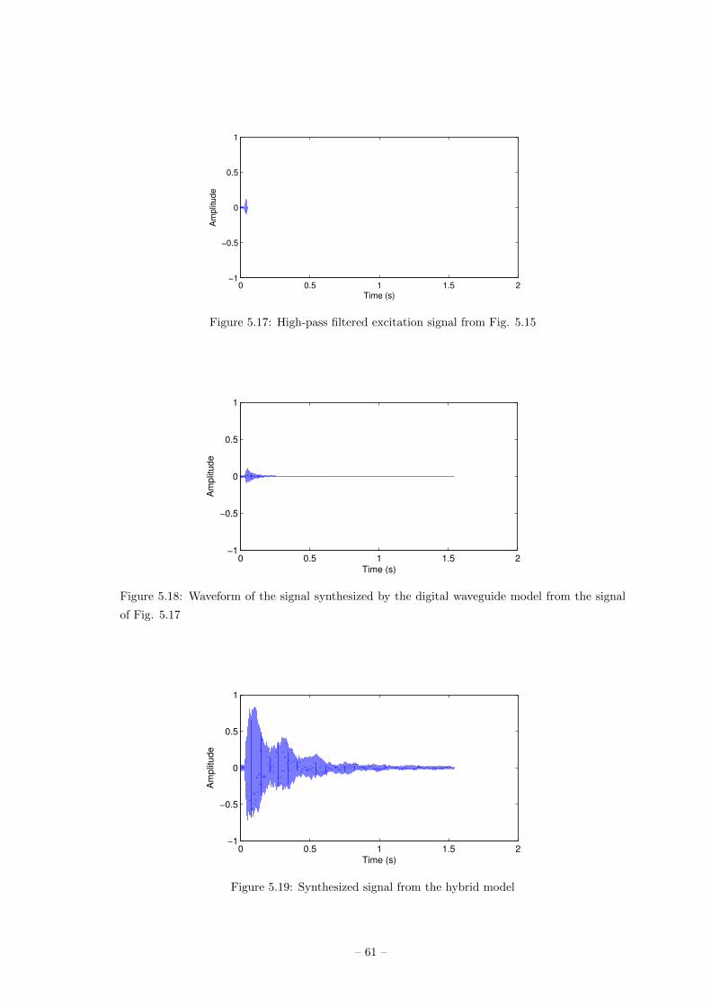
0 0.5 1 1.5 2−1

−0.5

0

0.5

1

Time (s)

Am

plit

ude

Figure 5.17: High-pass filtered excitation signal from Fig. 5.15

0 0.5 1 1.5 2−1

−0.5

0

0.5

1

Time (s)

Am

plit

ud

e

Figure 5.18: Waveform of the signal synthesized by the digital waveguide model from the signal

of Fig. 5.17

0 0.5 1 1.5 2−1

−0.5

0

0.5

1

Time (s)

Am

plit

ud

e

Figure 5.19: Synthesized signal from the hybrid model

– 61 –

Figure 5.20: STFT result of the signal of Fig. 5.19

0 500 1000 1500 2000 2500 3000−120

−100

−80

−60

−40

−20

Frequency (Hz)

Ma

gn

itu

de

(dB

)

Figure 5.21: Comparison of magnitude spectrums of the original geomungo tone (green curve) and

the synthesized geomungo tone (blue curve)

– 62 –

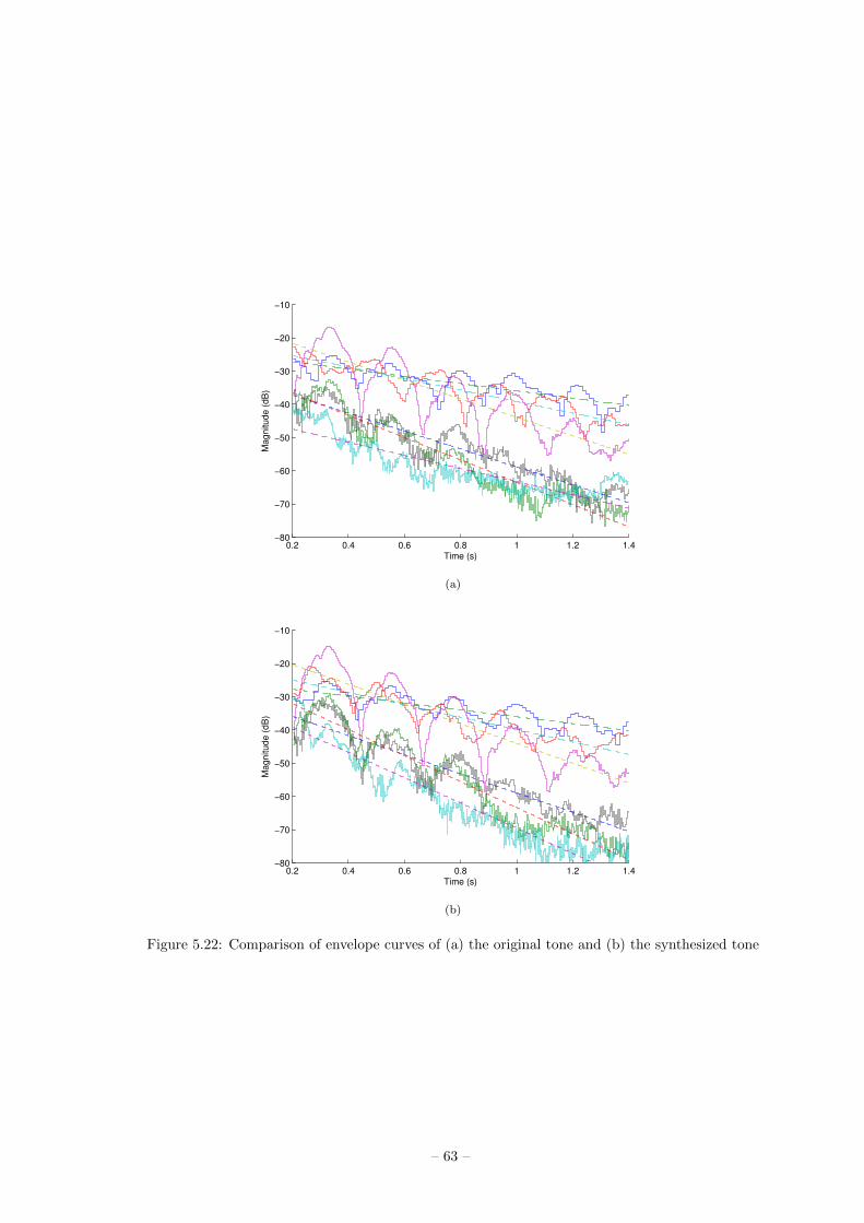
0.2 0.4 0.6 0.8 1 1.2 1.4−80

−70

−60

−50

−40

−30

−20

−10

Time (s)

Ma

gn

itu

de

(d

B)

(a)

0.2 0.4 0.6 0.8 1 1.2 1.4−80

−70

−60

−50

−40

−30

−20

−10

Time (s)

Ma

gn

itu

de

(d

B)

(b)

Figure 5.22: Comparison of envelope curves of (a) the original tone and (b) the synthesized tone

– 63 –

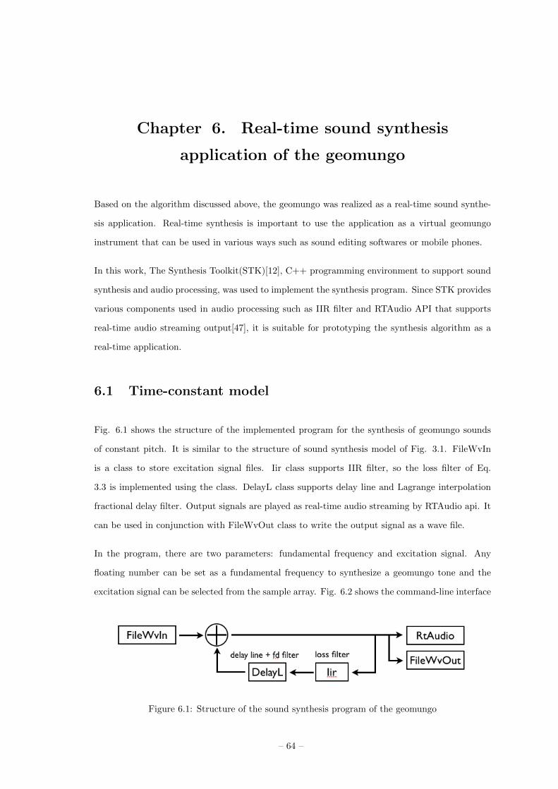
Chapter 6. Real-time sound synthesis

application of the geomungo

Based on the algorithm discussed above, the geomungo was realized as a real-time sound synthe-

sis application. Real-time synthesis is important to use the application as a virtual geomungo

instrument that can be used in various ways such as sound editing softwares or mobile phones.

In this work, The Synthesis Toolkit(STK)[12], C++ programming environment to support sound

synthesis and audio processing, was used to implement the synthesis program. Since STK provides

various components used in audio processing such as IIR filter and RTAudio API that supports

real-time audio streaming output[47], it is suitable for prototyping the synthesis algorithm as a

real-time application.

6.1 Time-constant model

Fig. 6.1 shows the structure of the implemented program for the synthesis of geomungo sounds

of constant pitch. It is similar to the structure of sound synthesis model of Fig. 3.1. FileWvIn

is a class to store excitation signal files. Iir class supports IIR filter, so the loss filter of Eq.

3.3 is implemented using the class. DelayL class supports delay line and Lagrange interpolation

fractional delay filter. Output signals are played as real-time audio streaming by RTAudio api. It

can be used in conjunction with FileWvOut class to write the output signal as a wave file.

In the program, there are two parameters: fundamental frequency and excitation signal. Any

floating number can be set as a fundamental frequency to synthesize a geomungo tone and the

excitation signal can be selected from the sample array. Fig. 6.2 shows the command-line interface

Figure 6.1: Structure of the sound synthesis program of the geomungo

– 64 –

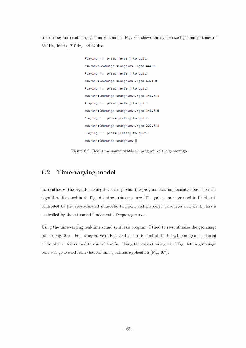
based program producing geomungo sounds. Fig. 6.3 shows the synthesized geomungo tones of

63.1Hz, 160Hz, 210Hz, and 320Hz.

Figure 6.2: Real-time sound synthesis program of the geomungo

6.2 Time-varying model

To synthesize the signals having fluctuant pitchs, the program was implemented based on the

algorithm discussed in 4. Fig. 6.4 shows the structure. The gain parameter used in Iir class is

controlled by the approximated sinusoidal function, and the delay parameter in DelayL class is

controlled by the estimated fundamental frequency curve.

Using the time-varying real-time sound synthesis program, I tried to re-synthesize the geomungo

tone of Fig. 2.1d. Frequency curve of Fig. 2.4d is used to control the DelayL, and gain coefficient

curve of Fig. 6.5 is used to control the Iir. Using the excitation signal of Fig. 6.6, a geomungo

tone was generated from the real-time synthesis application (Fig. 6.7).

– 65 –

(a)

(b)

(c)

(d)

Figure 6.3: Synthesized (a) 63.1Hz (b) 160Hz (c) 210Hz (d) 320Hz geomungo tones using the

real-time application

– 66 –

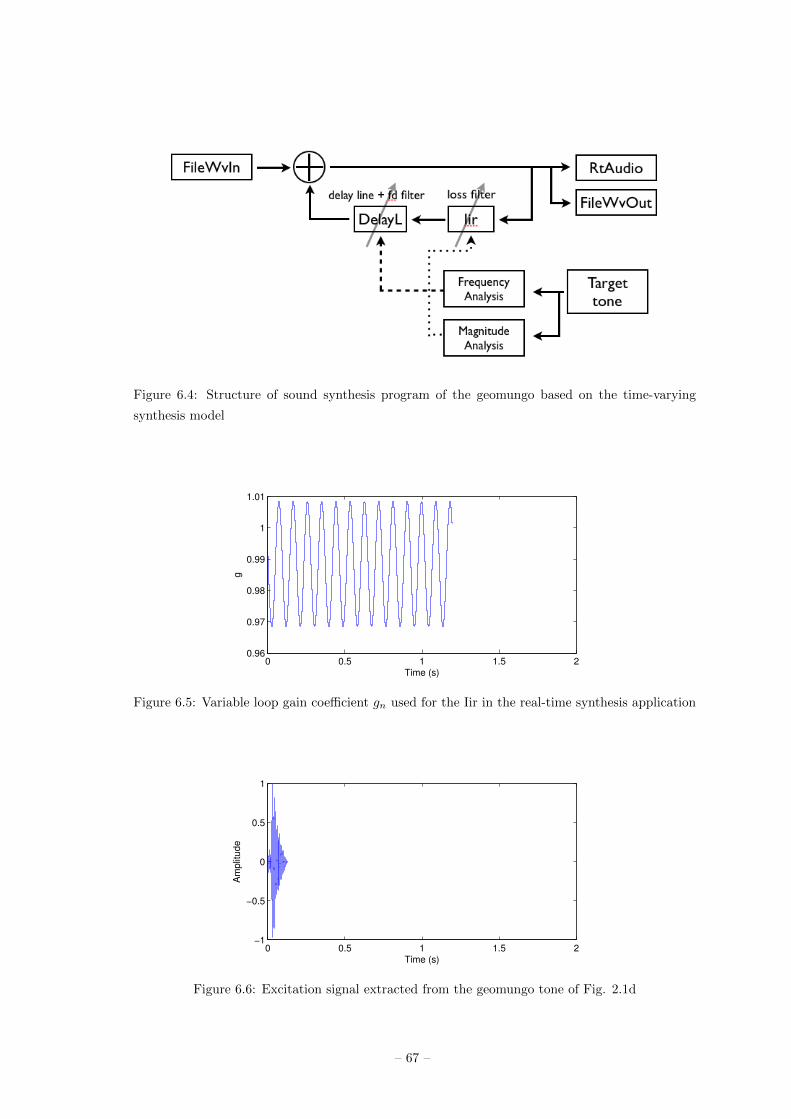
Figure 6.4: Structure of sound synthesis program of the geomungo based on the time-varying

synthesis model

0 0.5 1 1.5 20.96

0.97

0.98

0.99

1

1.01

Time (s)

g

Figure 6.5: Variable loop gain coefficient gn used for the Iir in the real-time synthesis application

0 0.5 1 1.5 2−1

−0.5

0

0.5

1

Time (s)

Am

plit

ude

Figure 6.6: Excitation signal extracted from the geomungo tone of Fig. 2.1d

– 67 –

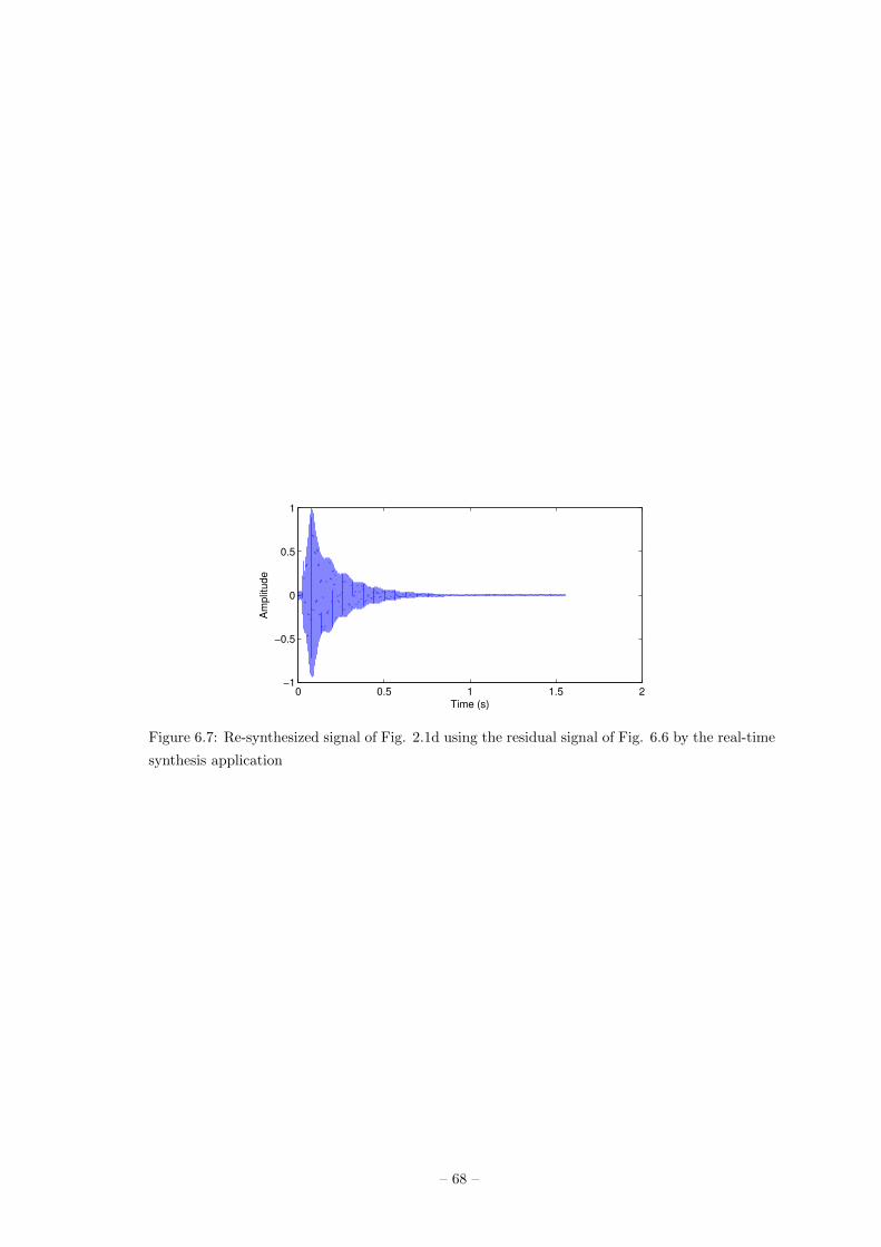
0 0.5 1 1.5 2−1

−0.5

0

0.5

1

Time (s)

Am

plit

ude

Figure 6.7: Re-synthesized signal of Fig. 2.1d using the residual signal of Fig. 6.6 by the real-time

synthesis application

– 68 –

Chapter 7. Conclusion

7.1 Evaluation

As a qualitative evaluation of the synthesized geomungo tones based on the digital waveguide

modeling, I interviewed an expert in Korean traditional music. After playing the original tones

and synthesized tones, I asked about the possibility of the proposed model to use in real music. She

answered that timbres of the synthesized tones were very similar to the original tones, but it was

better to add small noises because sounds played by the geomungo have some noises like friction.

In addition, she said that it was also better to synthesize more geomungo tones to generate various

kinds of vibrato effects.

In addition, a quantitative evaluation was performed based on an objective evaluation method.

In previous studies, group listening tests were used for evaluation of audio quality, but they are

subjective and time-consuming. Thus, research about object testing methods has been conducted.

For example, Perceptual Evaluation of Audio Quality (PEAQ) is the standardized assessment

method referred by the International Telecommunications Union (ITU). Perceptual Evaluation

of Speech Quality (PESQ) and Noise-To-Mask Ratio (NMR) are also the methods for objective

audio quality assessment[7]. However, these models were developed for digital speech coding for

wireless telephony or music coding for compression, so focuses of the models are different because

synthesized instrument tones sound different from a real instrument[17]. Nevertheless, there has

been a research for evaluating the waveguide synthesis method based on objective algorithms such

as Perceptual Audio Quality Measure (PAQM) and Noise-To-Mask Ratio (NMR)[63]. PAQM

algorithm showed that 71% of the scores fell within the range of scores of the human subjective

listening test. Thus, it is still doubtful whether the PAQM test assures the objective quality of the

synthesized tones, but I used the PAQM test to show that it is better to use the control of the gain

factor in the loop filter of the waveguide synthesis model based on a sinusoidal function. Because

the PAQM method scores based on difference between an original signal and a target signal based

on a human perception model, so getting high marks in the test means that the target signal is

more similar to the original signal.

Evaluation algorithm based on the PAQM test was implemented. The PAQM test includes com-

– 69 –

putation of spectral power density, transfer function of human ear model, transformation of the

samples from frequency to bark scale, time-domain spreading, and frequency-domain spreading.

Instructions of the PAQM test were in [5]. The final result from the PAQM test is a score from 1 to

5, and a lower score means that difference is smaller. Using the algorithm, synthesized tones were

scored based on the comparison of the original tones. As the test, the synthesized tone without

gain control (Fig. 4.8) scores 1.92, and the former with gain control (Fig. 4.15) scores 1.67. Thus,

synthesis of fluctuating geomungo tone with gain control is better. In addition, the synthesized

geomungo tone with another excitation signal (Fig. 4.16) scores 3.33, synthesized tone with the

hybrid model (Fig. 5.19) scores 2.3, and synthesized tone from the real-time application (Fig. 6.7)

scores 2.97.

7.2 Summary and conclusion

This paper discussed the sound synthesis of the geomungo, a Korean traditional plucked string

instrument. Physical modeling was used as a synthesis method for the instrument because it

allowed to generate various sounds based on mathematical models. Description of the geomungo

was discussed at first, and background theories about physical modeling were introduced.

From the extracted geomungo samples, frequency responses of the signals were estimated by

FFT and SFTF, and the harmonic partials were found from the magnitude spectrum. Then the

behaviors of fundamental frequency in time were estimated and some of them showed great pitch

fluctuations.

The model proposed in this work was based on the digital waveguide theory which was a generalized

Karplus-Strong algorithm. A ripple filter was used with a one-pole filter to design a loss filter,

and allpass filter was used to tune the fundamental frequency. Filter parameters were calibrated

by calculating the loss of the harmonic partials. Then input signals in the synthesis model were

calculated by inverse filtering from the recorded samples.

Synthesized geomungo tones sounds similar to original signals, and the peaks were found in the

magnitude spectrum. Then, in order to produce vibrato sounds having fluctuating pitches, an

time-varying synthesis model was proposed. The gain factor and loop gain coefficient in the loss

filter were controlled based on the magnitude analysis of the target tone, and the length of delay

line and fractional delay filter were controlled based on the frequency analysis of the target tone.

The variable gain coefficient was approximated as a sinusoid function. Excitation signal could be

– 70 –

extracted from a geomungo tone which had constant pitch and similar timbre to the target tone

or from the target tone itselft, but the latter needed to be modified by deamplifying and removing

the vibrating part in the sound.

For a more accurate synthesis, hybrid modal-waveguide synthesis which generated harmonic par-

tials at low frequencies with second-order resonators and at high frequencies with the digital

waveguide model. For fluctuant pitches, frequency and gain factor of each resonator was also

controlled by the frequency curve and the approximated gain coefficient curve of a sinusoidal func-

tion. The synthesized geomungo tone was very similar to the target tone in frequency domain

comparison.

Finally, a real-time sound synthesis application was realized by using STK. Using the application,

it could be possible to synthesize the geomungo tones of any fundamental frequency. The time-

varying model was also implemented for the vibrato sounds.

The model proposed in this work showed that physical modeling synthesis based on digital waveg-

uide theory was an effective method to generate the geomungo sounds which had various pitch

fluctuations. I expect that proposing sound synthesis models based on physical modeling for other

Korean traditional plucked string instruments is also highly effect. Ultimately, implementation

of a virtual synthesizer program which can be used in sound recording software is required for

composers to make use of the sounds of Korean traditional instruments without recording.

7.3 Future works

Future work includes the analysis of physical properties of each string and the design of a more

elaborate model considering nonlinear acoustic characteristics of geomungo tones. In real in-

strument, the relation between string and body is nonlinear. The proposed model in this work

assumed that it was linear and time invariant (LTI) because this made it possible to reduce the

computational cost. However, it may be better to design the body filter for realistic sounds. Also,

design of a model which generates an input signal is also necessary to synthesize model only based

on mathematical equations without any recorded samples. Finally, evaluation model for sound

synthesis methods of instruments needs to be established. Separation between music and noise

is important in audio compression, but generation and dissolution of harmonic partials are more

important in instrumental sounds. Thus, previous evaluation models need to be changed to result

in more accurate test scores.

– 71 –

References

[1] The geomungo. 국악과교육, 5:1–10, May 1982.

[2] Milton Abramowitz and Irene A. Stegun. Handbook of Mathematical Functions. Dover Pub-

lications, 1965.

[3] Jont B. Allen and Lawrence L. Rabiner. A unified approach to short-time fourier analysis

and synthesis. In Proceedings of the IEEE, volume 65, pages 1558–1564, November 1997.

[4] Balazs Bank, Federico Avanzini, Gianpaolo Borin, Giovanni De Poli, Federico Fontana, and

Davide Rocchesso. Physically informed signal processing methods for piano sound synthesis:

a research overview. EURASIP Journal on Applied Signal Processing, 2003:941–952, 2003.

[5] John G. Beerends. Audio quality determination based on perceptual measurement techniques,

chapter 1, pages 1–38. Applications of Digital Signal Processing to Audio and Acoustics.

Kluwer Academic Publishers, 1998.

[6] K. Bradley, Mu-Huo Cheng, and V.L. Stonick. Automated analysis and computationally

efficient synthesis of acoustic guitar strings and body. In Proceedings of the IEEE workshop

on Applied Signal Processing to Audio and Acoustics, pages 238–241, New Paltz, NY, USA,

October 1995.

[7] Dermot Campbell, Edward Jones, and Martin Glavin. Audio quality assessment techniques

- a review, and recent developments. Signal Processing, 89(8):1489–1500, 8 2009.

[8] Chris Chafe. A short history of digital sound synthesis by composers in the U.S.A.

[9] Sang-Jin Cho. Physical Modeling of the Sanjo Gayageum Using Digital Waveguide Theory.

PhD thesis, University of Ulsan, Ulsan, Korea, 2006.

[10] Sang-Jin Cho, Ui-Pil Chong, and Sang-Bock Cho. Synthesis of the dan trahn based on a

parameter extraction system. Journal of the Audio Engineering Society, 58(6):498–507, 2010.

[11] John Chowning. The synthesis of complex audio spectra by means of frequency modulation.

Journal of the Audio Engineering Society, 21(7):526–534, 1973.

– 72 –

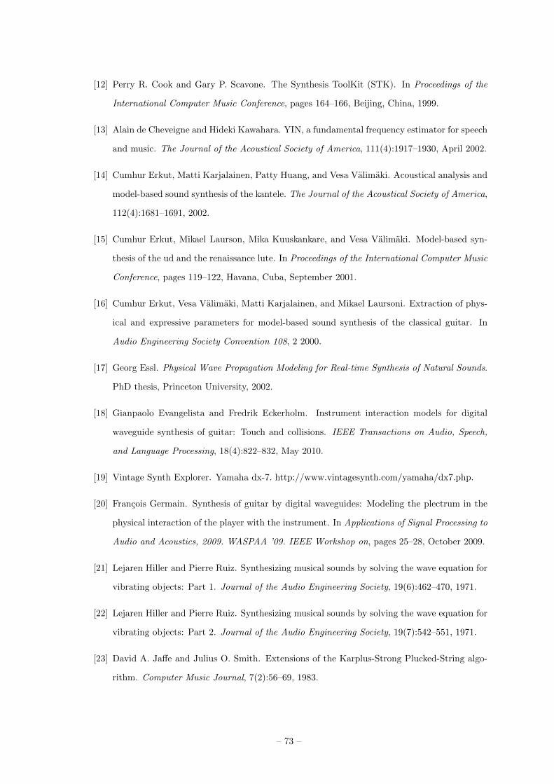
[12] Perry R. Cook and Gary P. Scavone. The Synthesis ToolKit (STK). In Proceedings of the

International Computer Music Conference, pages 164–166, Beijing, China, 1999.

[13] Alain de Cheveigne and Hideki Kawahara. YIN, a fundamental frequency estimator for speech

and music. The Journal of the Acoustical Society of America, 111(4):1917–1930, April 2002.

[14] Cumhur Erkut, Matti Karjalainen, Patty Huang, and Vesa Valimaki. Acoustical analysis and

model-based sound synthesis of the kantele. The Journal of the Acoustical Society of America,

112(4):1681–1691, 2002.

[15] Cumhur Erkut, Mikael Laurson, Mika Kuuskankare, and Vesa Valimaki. Model-based syn-

thesis of the ud and the renaissance lute. In Proceedings of the International Computer Music

Conference, pages 119–122, Havana, Cuba, September 2001.

[16] Cumhur Erkut, Vesa Valimaki, Matti Karjalainen, and Mikael Laursoni. Extraction of phys-

ical and expressive parameters for model-based sound synthesis of the classical guitar. In

Audio Engineering Society Convention 108, 2 2000.

[17] Georg Essl. Physical Wave Propagation Modeling for Real-time Synthesis of Natural Sounds.

PhD thesis, Princeton University, 2002.

[18] Gianpaolo Evangelista and Fredrik Eckerholm. Instrument interaction models for digital

waveguide synthesis of guitar: Touch and collisions. IEEE Transactions on Audio, Speech,

and Language Processing, 18(4):822–832, May 2010.

[19] Vintage Synth Explorer. Yamaha dx-7. http://www.vintagesynth.com/yamaha/dx7.php.

[20] Francois Germain. Synthesis of guitar by digital waveguides: Modeling the plectrum in the

physical interaction of the player with the instrument. In Applications of Signal Processing to

Audio and Acoustics, 2009. WASPAA ’09. IEEE Workshop on, pages 25–28, October 2009.

[21] Lejaren Hiller and Pierre Ruiz. Synthesizing musical sounds by solving the wave equation for

vibrating objects: Part 1. Journal of the Audio Engineering Society, 19(6):462–470, 1971.

[22] Lejaren Hiller and Pierre Ruiz. Synthesizing musical sounds by solving the wave equation for

vibrating objects: Part 2. Journal of the Audio Engineering Society, 19(7):542–551, 1971.

[23] David A. Jaffe and Julius O. Smith. Extensions of the Karplus-Strong Plucked-String algo-

rithm. Computer Music Journal, 7(2):56–69, 1983.

– 73 –

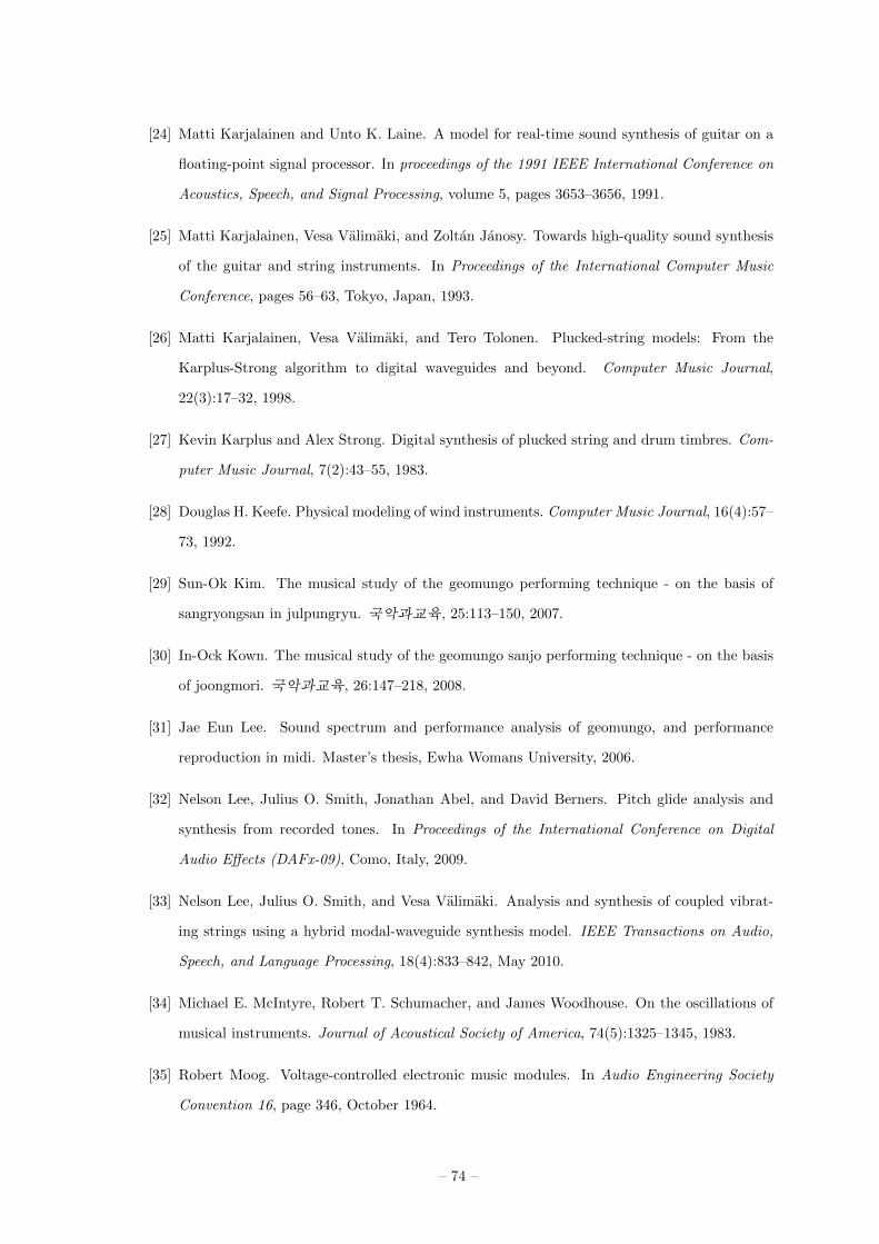
[24] Matti Karjalainen and Unto K. Laine. A model for real-time sound synthesis of guitar on a

floating-point signal processor. In proceedings of the 1991 IEEE International Conference on

Acoustics, Speech, and Signal Processing, volume 5, pages 3653–3656, 1991.

[25] Matti Karjalainen, Vesa Valimaki, and Zoltan Janosy. Towards high-quality sound synthesis

of the guitar and string instruments. In Proceedings of the International Computer Music

Conference, pages 56–63, Tokyo, Japan, 1993.

[26] Matti Karjalainen, Vesa Valimaki, and Tero Tolonen. Plucked-string models: From the

Karplus-Strong algorithm to digital waveguides and beyond. Computer Music Journal,

22(3):17–32, 1998.

[27] Kevin Karplus and Alex Strong. Digital synthesis of plucked string and drum timbres. Com-

puter Music Journal, 7(2):43–55, 1983.

[28] Douglas H. Keefe. Physical modeling of wind instruments. Computer Music Journal, 16(4):57–

73, 1992.

[29] Sun-Ok Kim. The musical study of the geomungo performing technique - on the basis of

sangryongsan in julpungryu. 국악과교육, 25:113–150, 2007.

[30] In-Ock Kown. The musical study of the geomungo sanjo performing technique - on the basis

of joongmori. 국악과교육, 26:147–218, 2008.

[31] Jae Eun Lee. Sound spectrum and performance analysis of geomungo, and performance

reproduction in midi. Master’s thesis, Ewha Womans University, 2006.

[32] Nelson Lee, Julius O. Smith, Jonathan Abel, and David Berners. Pitch glide analysis and

synthesis from recorded tones. In Proceedings of the International Conference on Digital

Audio Effects (DAFx-09), Como, Italy, 2009.

[33] Nelson Lee, Julius O. Smith, and Vesa Valimaki. Analysis and synthesis of coupled vibrat-

ing strings using a hybrid modal-waveguide synthesis model. IEEE Transactions on Audio,

Speech, and Language Processing, 18(4):833–842, May 2010.

[34] Michael E. McIntyre, Robert T. Schumacher, and James Woodhouse. On the oscillations of

musical instruments. Journal of Acoustical Society of America, 74(5):1325–1345, 1983.

[35] Robert Moog. Voltage-controlled electronic music modules. In Audio Engineering Society

Convention 16, page 346, October 1964.

– 74 –

[36] Robert Moog. Voltage-controlled electronic music modules. Journal of the Audio Engineering

Society, 13(3):200–206, 1965.

[37] 120 Years of Electronic Music. Elisha gray and “the musical telegraph”(1876).

http://120years.net/machines/telegraph/.

[38] Museum Portal of Korea. Geomungo. http://www.emuseum.go.kr.

[39] Alan V. Oppenheim and Ronald W. Schafer. Discrete-Time Signal Processing. Prentice Hall,

2009.

[40] Jyri Pakarinen, Matti Karjalainen, Vesa Valimaki, and Stefan Bilbao. Energy behavior in

time-varying fractional delay filters for physical modeling synthesis of musical instruments.

In Acoustics, Speech, and Signal Processing, 2005. Proceedings. (ICASSP ’05). IEEE Inter-

national Conference on, volume 3, pages iii/1–iii/4 Vol. 3, 2005.

[41] Henri Penttinen, Jyri Pakarinen, Vesa Valimaki, Mikael Laurson, Henbing Li, and Marc

Leman. Model-based sound synthesis of the guqin. The Journal of the Acoustical Society of

America, 120(6):4052–4063, 2006.

[42] Lawrence R. Rabiner. Theory and application of digital signal processing. Prentice Hall, 1975.

[43] Curtis Roads. The computer music tutorial. MIT Press, February 1996.

[44] Curtis Roads and Max Mathews. Interview with max mathews. Computer Music Journal,

4(4):15–22, 1980.

[45] Gary P. Scavone. Modeling wind instrument sound radiation using digital waveguide. In

Proceedings of the International Computer Music Conference, pages 355–358, Beijing, China,

1999.

[46] Gary P. Scavone and Perry R. Cook. Real-time computer modeling of woodwind instruments.

In Proceedings of the International Symposium on Musical Acoustics(ISMA), pages 197–202,

Leavenworth, Washington, U.S.A, 1998.

[47] Gary P. Scavone and Perry R. Cook. RtMidi, RtAudio, and a Synthesis ToolKit (STK) up-

date. In Proceedings of the International Computer Music Conference, pages 1–4, Barcelona,

Spain, 2005.

[48] Stefania Serafin and Diana Young. Recent advances in real-time bowed string synthesis:

Evaluation of the models. In Proceedings of the International Congress of Acoustics, Madrid,

Spain, 2007.

– 75 –

[49] Julius O. Smith. Waveguide filter tutorial. In Proceedings of the International Computer

Music Conference, pages 9–16, Champaign-Urbana, Illinois, U.S.A, 1987.

[50] Julius O. Smith. Physical modeling using digital waveguides. Computer Music Journal,

16(4):74–91, 1992.

[51] Julius O. Smith. Efficient synthesis of stringed musical instruments. In Proceedings of the

International Computer Music Conference, pages 64–71, Tokyo, Japan, 1993.

[52] Julius O. Smith. Principles of digital waveguide models of musical instruments. Applications

of Digital Signal Processing to Audio and Acoustics, 437:417–466, 2002.

[53] Julius O. Smith. Mathematics of the discrete fourier transform(DFT). W3K Publishing,

2003.

[54] Julius O. Smith and Scott A. Van Duyne. Commuted piano synthesis. In Proceedings of the

International Computer Music Conference, pages 319–326, 1995.

[55] Sound On Sound. Yamaha VL1. http://www.soundonsound.com/sos/1994 articles/jul94/yama

havl1.html.

[56] Gilbert Strang. Linear Algebra and Its Applications. Harcourth Brace Jovanovich, 1988.

[57] Tero Tolonen, Vesa Valimaki, and Matti Karjalainen. Modeling of tension modulation nonlin-

earity in plucked strings. IEEE Transactions on Speech and Audio Processing, 8(3):300–310,

2000.

[58] Vesa Valimaki. Discrete-Time Modeling of Acoustic Tubes Using Fractional Delay Filters.

PhD thesis, Helsinki University of Technology, Espoo, Finland, 1995.

[59] Vesa Valimaki, Jyri Huopaniemi, and Matti Karjalainen. Physical modeling of plucked string

instruments with application to real-time sound synthesis. Journal of the Audio Engineering

Society, 44(5):331–352, 1996.

[60] Vesa Valimaki, Timo I. Laakso, and J. Mackenzie. Elimination of transients in time-varying

allpass fractional delay filters with application to digital waveguide modeling. In Proceedings

of the International Computer Music Conference, pages 327–334, Banff, Alberta, Canada,

September 1995.

[61] Vesa Valimaki, Henri Penttinen, Jonte Knif, Mikael Laurson, and Cumhur Erkut. Sound

synthesis of the harpsichord using a computationally efficient physical model. EURASIP

Journal on Applied Signal Processing, 2004:934–948, 2004.

– 76 –

[62] Vesa Valimaki and Tero Tolonen. Development and calibration of a guitar synthesizer. Journal

of the Audio Engineering Society, 46(9):766–778, 1998.

[63] Steve G. Wood. Objective test methods for waveguide audio synthsis. Master’s thesis,

Brigham Young University, 2007.

[64] James Woodhouse. Physical modeling of bowed strings. Computer Music Journal, 16(4):43–

56, 1992.

– 77 –

Acknowledgement

– 78 –

이 력 서

이 름 : 김 승 훈

생 년 월 일 : 1988년 4월 23일

주 소 : 부산광역시 해운대구 반여4동 우방신세계타운 105-1806

E-mail 주 소 : [email protected]

학 력

2004. 3. – 2006. 2. 부산과학고등학교

2006. 2. – 2009. 2. 한국정보통신대학교(ICU) 전자통신공학과 (B.S.)

2009. 2. – 2011. 8. 한국과학기술원(KAIST) 문화기술대학원 (M.S.)

경 력

2007. 8. – 2008. 2. 핀란드 탐페레공과대학 (Tampere University of Technology) 교환학생

2010. 9. – 2010. 12. GCT 633 Audio & Multimedia Programming 과목조교

연구업적

1. Jeho Oh, Soyoung Kim, Seunghun Kim, and Chungkon Shi. A Study of Interactive Art in

the Narrative Form of ”Magic Monkey”, In Proceedings of the 8th International Conference

on Computer Graphics, Imaging, and Visualization, Singapore, August, 2011.

2. Seunghun Kim and Woon Seung Yeo. Musical Control of a Pipe Based on Acoustic Reso-

nance, In Proceedings of the International Conference on New Interfaces for Musical Expres-

sion, Oslo, Norway, Jun, 2011.

– 79 –

3. Seunghun Kim, Luke Keunhyung Kim, Songhee Jeong, and Woon Seung Yeo. Clothesline

as a Metaphor for a Musical Interface, In Proceedings of the International Conference on New

Interfaces for Musical Expression, Oslo, Norway, Jun, 2011.

4. Seunghun Kim, Jooseok Hong, Jinwoo Kim, Soyoung Kim, and Woon Seung Yeo, Emotional

Expression in Online Communication Based on Physiological Siganls, In Proceedings of the

Korean Conference of HCI, Pyeongchang, Korea, January, 2011.

5. Seunghun Kim and Woon Seung Yeo, Clothesline-based Interactive Music Installation, Jour-

nal of the engineering and arts society in Korea, 2010.

6. Sihwa Park, Seunghun Kim, Samuel Lee, and Woon Seung Yeo, Online Map Interface for

Creative and Interactive Music-Making, In Proceedings of the International Conference on

New Interfaces for Musical Expression, Sydney, Australia, June, 2010.

7. Sihwa Park, Seunghun Kim, Samuel Lee, and Woon Seung Yeo, Composition With Path:

Musical Sonification of Geo-referenced Data With Online Map Interface, In Proceedings of

the International Computer Music Conference, New York, NY, USA, June, 2010.

8. Sihwa Park, Seunghun Kim, Samuel Lee, and Woon Seung Yeo, COMPath: Music Compo-

sition Environment Based on Interactive Map Interface, In Proceedings of the Korean Elec-

troacoustic Music Society Conference, Seoul, Korea, December, 2009.

– 80 –

sound synthesis of the geomungo using digital waveguide ... filesound synthesis of the geomungo...

Documents