statistics of wind and waves off tsuyazaki, fukuoka, in ... · akira masuda, tadao kusaba, kenji...

Journal of Oceanography, Vol. 55, pp. 289 to 305. 1999

289Copyright The Oceanographic Society of Japan.

Keywords:⋅Statistics of windsand waves,

⋅Eastern TsushimaStrait,

⋅ seasonal cycle,⋅upper bound ofwave steepness,

⋅ spectral similaritybetween winds andwaves.

Statistics of Wind and Waves off Tsuyazaki, Fukuoka,in the Eastern Tsushima Strait

AKIRA MASUDA, TADAO KUSABA, KENJI MARUBAYASHI and MICHIYOSHI ISHIBASHI

Research Institute for Applied Mechanics, Kyushu University, Kasuga 816, Japan

(Received 9 September 1998; in revised form 5 November 1998; accepted 13 November 1998)

The variability of the sea surface wind and wind waves in the coastal area of the EasternTsushima Strait was investigated based on the hourly data from 1990 to 1997 obtained ata station 2 km off Tsuyazaki, Fukuoka. The annual mean wind speed was 4.84 m s–1, withstrong northwesterly monsoon in winter and weak southwesterly wind in summer.Significant wave heights and wave periods showed similar sinusoidal seasonal cyclesaround their annual means of 0.608 m and 4.77 s, respectively. The seasonal variabilityrelative to the annual mean is maximum for wave heights, medium for wind speeds, andminimum for wave periods. Significant wave heights off Tsuyazaki turned out to bebounded by a criterion, which is proportional to the square of the significant wave periodcorresponding to a constant steepness, irrespective of the season or the wind speed. Forterms shorter than a month, the significant wave height and the wave period were foundto have the same spectral form as the inshore wind velocity: white for frequencies less than0.2 day–1 and proportional to the frequency to the –5/3 power for higher frequencies,where the latter corresponds to the inertial subrange of turbulence. The spectral levels ofwave heights and wave periods in that inertial range were also correlated with those of theinshore wind velocity, though the scatter was large.

measured once an hour since 1989 at a sea observation toweroff Tsuyazaki, Fukuoka, by the Research Institute for Ap-plied Mechanics (RIAM), Kyushu University. Since noother similar station is located nearby, the data obtainedthere have been considered the most reliable concerning thesea surface wind and wind waves of the coastal area of theEastern Tsushima Strait. The data obtained at the station willcontinue to supply valuable information not only for thefundamental science of air-sea interaction, but also for aprojected plan of the Japan Sea, which is considered as anideal field for the experiment of monitoring and predictingthe oceanic and atmospheric variability (Masuda, 1998).

No systematic analysis, however, has been publishedeven for the basic features of the sea surface wind and windwaves at that location representing the Eastern TsushimaStrait. For future research, therefore, the present paperprepares the basic statistics or the climatology of the seasurface wind and wind waves based on the direct measure-ment at the fixed station representative of the EasternTsushima Strait.

In the next section a brief sketch is given of theobservation system and the preliminary data processing.The third section then yields overall statistics of the seasurface wind and waves based on the eight years of obser-vation: time series, annual means, and seasonal variation aswell as scatter diagrams. The short-term variability is dis-

1. IntroductionIn order to forecast the variability of the ocean it is quite

important to estimate the air-sea flux precisely. Amongvarious factors governing the air-sea interaction, the seasurface wind is probably the most fundamental; the seasurface wind appears in every bulk formula for the exchangeof momentum, heat, and various kinds of material, includingcarbon dioxide, between the ocean and the atmosphere.

Recently wind waves have been widely recognized asanother key element that controls the air-sea interaction,because wind waves represent the sea surface state orroughness. The subject has been argued intensively for thelast ten years or so, in particular as regards the surfaceroughness z0, which is equivalent to the drag coefficient ofthe sea surface under the neutrally stratified air just abovethe sea surface (Masuda and Kusaba, 1987; Toba et al., 1990;Donelan, 1993). See Komen et al. (1998) for a most recentreview of this problem. Nevertheless the issue has remainedconfused. To settle this complicated and important problem,further elaborate observation is needed for qualified andreliable data of the sea surface wind and wind waves (forexample, the HEXOS experiment reported by Smith et al.,1992). In this sense a fixed observation station is especiallyvaluable to accumulate long-term records of such randomvariables in the field measurement.

The sea surface wind and wind waves have been

290 A. Masuda et al.

Fig. 1. Location of the Tsuyazaki Sea Observation Station, whichis 2 km northwest off Tsuyazaki, Fukuoka, in the EasternTsushima Strait. The tower stands on a bottom which is 15 mdeep lying over a gentle slope of 1/100–2/100.

cussed in the fourth section, where spectral similarity isfound among the inshore wind velocity, significant waveheights, and significant wave periods. Finally the fifthsection gives a summary and discussion.

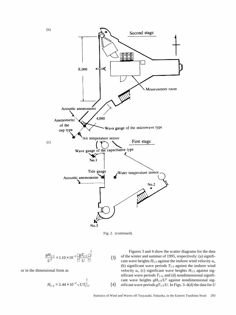
2. Observation System and Preliminary Data Process-ingFigure 1 shows the location of the sea observation

tower 2 km northwestward off Tsuyazaki, Fukuoka. Thetower stands on a bottom which is 15 m deep lying over agentle slope of 1/100–1/200. With the open ocean to thenorthwest, the tower provides an ideal station for measuringwind waves developed by the northwest winter monsoon.Moreover, it is the only fixed station for measuring themaritime condition of the Eastern Tsushima Strait.

Figure 2 illustrates the observation system at the tower.The wind speed and wind direction are measured by ananemometer of the propeller type with a vane at a height of17 m from the mean sea surface. Waves are measured asfollows. First the Doppler shift due to the vertical dis-placement of the sea surface is measured by a microwavewave gauge, the electromagnetic horn of which is fixed at apoint protruding 4 m southwestward from the second stageof the tower. The measured Doppler shift gives the verticalvelocity of the sea surface, from which the surface elevationis calculated through time integration.

In the routine measurement, both the wind and thesurface displacement are sampled at a frequency of 20 Hzfor the first 12 minutes of every one hour period. Wave

heights and wave periods are calculated from the surfacedisplacement by the zero-up-cross method. The hourly dataconcerned here are the 12 minute mean wind speed U, 12minute mean wind direction θ, 12 minute maximum windspeed Umax, wind direction at that moment θmax, significantwave height H1/3, significant wave period T1/3, 12 minutemaximum wave height Hmax, and 12 minute maximum waveperiod Tmax, which is the wave period for the wave of Hmax.Wave variables are based on the 12 minute record of surfacedisplacement, which contains more than 140 waves for atypical wave period of 5 s. This number of waves yields theexpected mode of the maximum wave height as

Hmax =2 log140

πH1/3

1.60= 1.57 × H1/3 1( )

(Longuet-Higgins, 1952).The data processed as above at the tower are transferred,

together with other data such as those of tide levels, by anonline telemeter system to the Tsuyazaki Maritime Labo-ratory of the RIAM. For details of the instruments, pre-liminary data processing, and the ocean data telemeteringsystem, see Marubayashi et al. (1989) and the Annual Re-ports of Oceanographic Data at the Tsuyazaki Station (1989–1997), the Dynamics Simulations Research Center, RIAM,Kyushu University.

From the raw data, the hourly wind vector (uE, uN) iscalculated from U and θ: the eastward and northwardcomponents of wind are defined by uE = Ucosθ and uN =Usinθ, where θ is measured anticlockwise from the east.Note that θ is the direction to which the wind is blowing. Wealso use the inshore and alongshore wind velocities ui and ua,which are the northwesterly and southwesterly componentsof the wind vector defined by ui ≡ Ucos(θ + π/4) and ua ≡Usin(θ + π/4); the northwest direction is the outward normalto the coast. The positive inshore wind velocity is probablythe most responsible for the growth of wind waves observedat the Tsuyazaki Station.

For the convenience of the later analysis, we classifythe four seasons of winter, spring, summer, and autumn, asthe months of December to February, March to May, June toAugust, and September to November, respectively. This isbecause the wind and wave characteristics depend on theseason.

3. Fundamental Statistics and Seasonal Variation

3.1 Annual means, yearly maxima and scatter diagramsThe simple mean or annual mean of the hourly scalar

wind speed U over the eight years from 1990 to 1997 was4.84 m s–1. The mean of the wind vector based on the 12minute wind speed and wind direction was (0.54, –0.68) ms–1 in terms of the zonal and meridional representation,

Statistics of Wind and Waves off Tsuyazaki, Fukuoka, in the Eastern Tsushima Strait 291

while it was (0.86, –0.10) m s–1 in terms of the inshore andalongshore decomposition. The annual mean wind blowsalmost inshore on account of the large contribution from thenorthwesterly winter monsoon. Also note that the magni-tude of the annual mean of the wind vector is below a fifthof the annul mean of the scalar wind speed U. As regardswave properties, the annual mean was 0.608 m for signifi-cant wave heights H1/3 and 4.77 s for significant wave peri-ods T1/3.

Another useful statistic is the yearly maximum value,because disasters often occur together with strong winds andhigh waves. It was determined as the maximum among oneyear of hourly data. Tables 1 and 2 respectively show theyearly maxima of the wind speed and wave height thusdetermined, along with other wind and wave propertieswhen the maxima occurred. The highest wind speed observedfrom 1990 to 1997 was 51.1 m s–1 associated with a fiercetyphoon of September in 1991, for which even the 12 minutemean wind speed was 36.4 m s–1. That typhoon, however,

did not cause the maximum wave height; the duration isshort and the wind direction changes rapidly for a typhoonin general. Instead, the maximum wave height of 5.12 mappeared in January of 1997, when the strong wind blewalmost from the west.

We see that the yearly maximum wind speed is ratherrandom; the range is wide and the corresponding winddirection is irregular. On the other hand, the yearly maxi-mum wave height is stable, concentrated around 4.8 m withperiods of 6 to 7 s. They occurred with the westerly tonorthwesterly wind in winter from December to March. Anexception was found in 1990, when the wind blew from thenorth in September: Hmax < 4 m and Tmax > 8 s. Probably themaximum wave height in 1990 was due to swells comingfrom the north.

Next let us investigate the correlation among the threevariables of U, H1/3, and T1/3. Since it is the wind that gen-erates wind waves, some degree of correlation is expectedeither between H1/3 and U or between T1/3 and U, through the

year/month/day/time Hmax Tmax U θ H1/3 T1/3 Umax θmax

(m) (s) (m s –1 ) (deg.) (m) (s) (m s –1) (deg.)

’90/09/19/23 3.96 8.3 14.5 350 2.55 8.8 19.4 353’90/12/11/10 4.76 6.6 20.0 276 1.97 7.0 25.1 280’92/01/31/23 4.81 6.7 20.9 217 2.7 6.7 27.5 225’93/01/28/03 4.86 6.8 16.1 305 2.56 7.1 20.0 309’94/02/10/02 4.81 6.5 12.6 292 2.24 6.8 16.4 286’95/03/11/02 4.69 7.3 15.3 276 2.5 7.2 20.1 272’96/02/05/12 4.85 5.6 15.2 273 2.24 6.0 19.5 266’97/01/01/19 5.12 6.3 17.7 275 2.65 6.7 22.8 271

Table 2. The same as Table 2 except that the yearly maximum is for the wave height Hmax, so that the second and the fifth columnsare exchanged.

year/month/day/time Umax θmax U θ H1/3 T1/3 Hmax Tmax

(m s –1) (deg.) (m s –1) (deg.) (m) (s) (m) (s)

’90/09/19/09 28.5 27 19.1 11 1.54 5.9 2.22 5.8’91/09/27/19 51.1 302 36.4 301 3.07 6.5 4.29 6.6’92/08/08/13 39.3 357 28.1 342 1.93 6.0 2.89 4.8’93/08/10/01 33.4 88 21.7 90 0.81 3.4 1.17 3.3’94/10/12/06 34.7 191 24.7 183 1.43 4.1 1.92 4.2’95/11/07/21 26.8 268 20.0 277 2.95 7.1 4.34 6.4’96/08/14/11 30.5 37 22.9 31 0.87 2.8 1.38 2.7’97/09/16/15 28.7 357 20.2 11 1.86 3.9 1.27 3.0

Table 1. The yearly maximum among hourly 12 minute maxima of wind speed Umax for each year from 1990 to 1997, together withconditions when the yearly maximum wind speed was observed: the first column shows the date and time when the maximum wasobserved, the second the maximum wind speed Umax and the wind direction θmax at that time, the third the mean wind speed U andthe mean wind direction θ, the fourth the significant wave height H1/3 and the significant wave period T1/3, and the fifth the maximumwave height Hmax and the maximum wave period Tmax. Here the wind direction is expressed in a conventional way; it is the directionthe wind comes from and measured clockwise from the north in degrees.


fetch relations (Mitsuyasu, 1968, 1969; Hasselmann et al.,1973):

H1/3 = 1.99 ×10−3 F

gU = 6.37 ×10−4 F ⋅U

T1/3 = 3.21×10−1 F

g2

1

3U

1

3 = 7.00 ×10−2 F1

3U1

3 ,

2( )

Fig. 2. Sketch of the observation system at the Tsuyazaki Station: (a) the side view of the tower, (b) the plan view of the second stage,and (c) the plan view of the first stage. The length is in units of mm.

where F is the fetch and g = 9.8 m s–2 the acceleration dueto gravity. Here we have put U ≡ U17 = 1.053 × U10 based onthe assumption of a constant drag coefficient of 1.6 × 10–3

for U10, where U17 and U10 denote the wind speeds at heightsof 17 m and 10 m, respectively. Also wave heights and waveperiods are expected to be related with each other throughthe 3/2-power law of Toba (1972), which is obtained whenF is eliminated from the fetch relations (2). It is expressed inthe nondimensional form as

(a)


gH1/3

U 2 = 1.10 ×10−2 gT1/3

U

3

23( )

or in the dimensional form as

H1/3 = 3.44 ×10−2 UT1/3

3

2 . 4( )

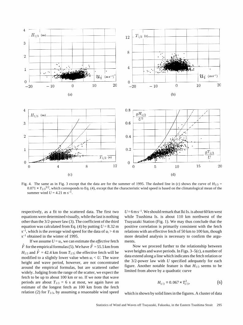
Figures 3 and 4 show the scatter diagrams for the dataof the winter and summer of 1995, respectively: (a) signifi-cant wave heights H1/3 against the inshore wind velocity ui,(b) significant wave periods T1/3 against the inshore windvelocity ui, (c) significant wave heights H1/3 against sig-nificant wave periods T1/3, and (d) nondimensional signifi-cant wave heights gH1/3/U2 against nondimensional sig-nificant wave periods gT1/3/U. In Figs. 3–4(d) the data for U

(b)

(c)

Fig. 2. (continued).


≤ 4 m s–1 are excluded to avoid the division by an inad-equately small value of U. As a whole it is difficult to findsimple relations either between H1/3 and ui or between T1/3

and ui, in particular for negative ui in summer. Nevertheless,a positive correlation is found between H1/3 and ui in thepositive ui region for the winter data. Correlation is lessobvious, however, between T1/3 and ui even in the positiveui region in winter. Significant wave heights H1/3 and sig-nificant wave periods T1/3 are correlated well with eachother in winter, though the scatter is large. Whennondimensionalized in terms of g and U, significant waveheights and significant wave periods are correlated muchbetter, both in winter and in summer.

For a while let us concentrate our attention on thewinter data of positive ui of a medium to high speed, for

(b)(a)

(c) (d)

Fig. 3. Scatter diagrams for the winter of 1995: (a) significant wave heights H1/3 versus the inshore wind velocity ui, (b) significantwave periods T1/3 versus the inshore wind velocity ui, (c) significant wave heights H1/3 versus significant wave periods T1/3, and(d) nondimensional significant wave heights gH1/3/U2 versus nondimensional significant wave periods gT1/3/U, where g is theacceleration due to gravity g and U the wind speed; in (d) the data for U ≤ 4 m s–1 were excluded. The lines in (c) show the scalinglaws: a solid line for Eq. (6), a dotted line for Eq. (8), and a dashed line for H1/3 = 0.083 × T1/3

3/2. The last line corresponds to Eq.(4) except that the characteristic wind speed is based on the climatological mean of the winter wind U = 5.86 m s–1.

which we observe significant correlation with wave proper-ties. Figure 5 replots the winter case of Fig. 3 on logarithmicscales, where we have excluded the data when ui ≤ 4 m s–1.The lines drawn indicate

H1/3 = 0.15 × ui

T1/3 = 2.44 × ui

1

3

H1/3 = 0.099 × T1/3

3

2

gH1/3

U 2 = 0.011×gT1/3

U

3

2,

5( )


(a) (b)

(c) (d)

respectively, as a fit to the scattered data. The first twoequations were determined visually, while the last is nothingother than the 3/2-power law (3). The coefficient of the thirdequation was calculated from Eq. (4) by putting U = 8.32 ms–1, which is the average wind speed for the data of ui > 4 ms–1 obtained in the winter of 1995.

If we assume U = ui, we can estimate the effective fetch

F for the empirical formulas (5). We have

F = 55.5 km from

H1/3 and

F = 42.4 km from T1/3; the effective fetch will bemodified to a slightly lower value when ui < U. The waveheight and wave period, however, are not concentratedaround the empirical formulas, but are scattered ratherwidely. Judging from the range of the scatter, we expect thefetch to be up to about 100 km or so. If we note that waveperiods are about T1/3 = 6 s at most, we again have anestimate of the longest fetch as 100 km from the fetchrelation (2) for T1/3, by assuming a resaonable wind speed

U = 6 m s–1. We should remark that Iki Is. is about 60 km westwhile Tsushima Is. is about 110 km northwest of theTsuyazaki Station (Fig. 1). We may thus conclude that thepositive correlation is primarily consistent with the fetchrelations with an effective fetch of 50 km to 100 km, thoughmore detailed analysis is necessary to confirm the argu-ments.

Now we proceed further to the relationship betweenwave heights and wave periods. In Figs. 3–5(c), a number ofdata extend along a line which indicates the fetch relation orthe 3/2-power law with U specified adequately for eachfigure. Another notable feature is that H1/3 seems to belimited from above by a quadratic curve

H1/3 = 0.067 × T1/32 , 6( )

which is shown by solid lines in the figures. A cluster of data

Fig. 4. The same as in Fig. 3 except that the data are for the summer of 1995. The dashed line in (c) shows the curve of H1/3 =0.071 × T1/3

3/2, which corresponds to Eq. (4), except that the characteristic wind speed is based on the climatological mean of thesummer wind U = 4.21 m s–1.


(a) (b)

(c) (d)

Fig. 5. The same as in Fig.3 except that the data of ui ≤ 4 m s–1 are excluded and the results are shown on logarithmic scales. The linesin (a) and (b) respectively indicate the empirical relations fitted visually: H1/3 = 0.15 × ui and T1/3 = 2.44 × ui

1/3. In (c) and (d), thesolid line shows the empirical upper bound found here (6), the dotted line the steepness for the saturated sea by Wilson (8), and thedashed line the 3/2-power law of H1/3 = 0.0099 × T3/2 for (c) or gH1/3/U2 = 0.011 × (gT1/3/U)3/2 for (d), respectively.

are found close to this upper bound. In logarithmic scales ofFig. 5(c) the upper limit becomes conspicuous, making astraight boundary to the data. For nondimensionalized waveheights and wave periods, Fig. 5(d) indicates the data nearthe upper bound are mostly of young waves characterized bya small wave age gT1/3/U. The upper bound applies to olderwaves as well, though the number is small.

The T1/3-square dependence of the right-hand side ofEq. (6) suggests that the upper bound is independent of theinshore wind velocity. A candidate for the mechanismsrelated with the constraint is the breaking condition ofgravity waves described by Michell (1893), which is ex-pressed as H/L = 1/7 for a regular wave of wave height H andwave length L. It is rewritten as

H1/3 = 0.223 × T1/32 7( )

if we identify H with H1/3 and T with T1/3, respectively, forconvenience. Another possibility is the wave height for thefully developed sea expected from the Wilson IV formula(Wilson, 1965)

H1/3 = 0.0397 × T1/32 , 8( )

which is indicated by a dotted line in the figures. The dottedline crosses with the dashed line representing the 3/2-powerlaw at a point, which usually means the saturated state ofwaves. Note, however, that the data extend a little furtheralong the line of the 3/2-power law. The coefficient of (6)found here is above that of (8) and below that of (7).

To our surprise, Eq. (6) was confirmed to apply to mostdata obtained at the Tsuyazaki Station, irrespective of theseason or the wind speed. A question is whether Eq. (6) is


applicable to the wave data of other similar stations. Or isthis curve peculiar to the data of the station off Tsuyazaki?What kind of physics is responsible for that? We know that,at least, much younger wind waves in a wind flume can havea steepness larger than that given by Eq. (6). They are stillbounded by the limiting steepness equivalent to Eq. (7)(Kusaba and Masuda, 1989). Also an inspection shows thatsome individual waves in a wind flume analyzed by Koga(1984) have wave heights that are very close to the breakingcondition of Eq. (7). The questions mentioned above may beanswered by carrying out similar analyses for other sourcesof wind and wave data.

3.2 Seasonal variationWe next investigate the seasonal variation using the

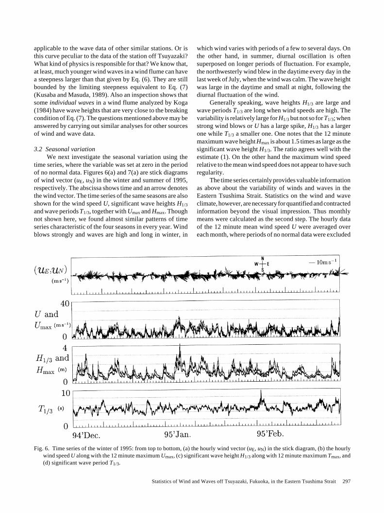
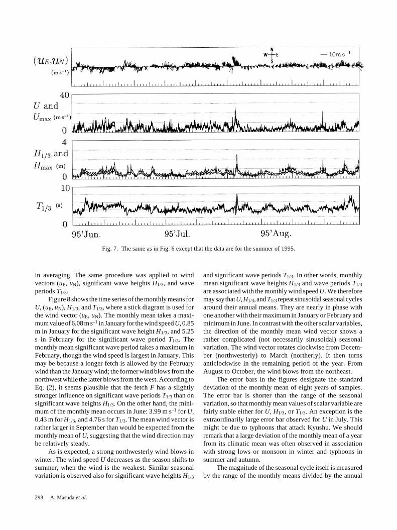
time series, where the variable was set at zero in the periodof no normal data. Figures 6(a) and 7(a) are stick diagramsof wind vector (uE, uN) in the winter and summer of 1995,respectively. The abscissa shows time and an arrow denotesthe wind vector. The time series of the same seasons are alsoshown for the wind speed U, significant wave heights H1/3

and wave periods T1/3, together with Umax and Hmax. Thoughnot shown here, we found almost similar patterns of timeseries characteristic of the four seasons in every year. Windblows strongly and waves are high and long in winter, in

which wind varies with periods of a few to several days. Onthe other hand, in summer, diurnal oscillation is oftensuperposed on longer periods of fluctuation. For example,the northwesterly wind blew in the daytime every day in thelast week of July, when the wind was calm. The wave heightwas large in the daytime and small at night, following thediurnal fluctuation of the wind.

Generally speaking, wave heights H1/3 are large andwave periods T1/3 are long when wind speeds are high. Thevariability is relatively large for H1/3 but not so for T1/3; whenstrong wind blows or U has a large spike, H1/3 has a largerone while T1/3 a smaller one. One notes that the 12 minutemaximum wave height Hmax is about 1.5 times as large as thesignificant wave height H1/3. The ratio agrees well with theestimate (1). On the other hand the maximum wind speedrelative to the mean wind speed does not appear to have suchregularity.

The time series certainly provides valuable informationas above about the variability of winds and waves in theEastern Tsushima Strait. Statistics on the wind and waveclimate, however, are necessary for quantified and contractedinformation beyond the visual impression. Thus monthlymeans were calculated as the second step. The hourly dataof the 12 minute mean wind speed U were averaged overeach month, where periods of no normal data were excluded

Fig. 6. Time series of the winter of 1995: from top to bottom, (a) the hourly wind vector (uE, uN) in the stick diagram, (b) the hourlywind speed U along with the 12 minute maximum Umax, (c) significant wave height H1/3 along with 12 minute maximum Tmax, and(d) significant wave period T1/3.


Fig. 7. The same as in Fig. 6 except that the data are for the summer of 1995.

in averaging. The same procedure was applied to windvectors (uE, uN), significant wave heights H1/3, and waveperiods T1/3.

Figure 8 shows the time series of the monthly means forU, (uE, uN), H1/3, and T1/3, where a stick diagram is used forthe wind vector (uE, uN). The monthly mean takes a maxi-mum value of 6.08 m s–1 in January for the wind speed U, 0.85m in January for the significant wave height H1/3, and 5.25s in February for the significant wave period T1/3. Themonthly mean significant wave period takes a maximum inFebruary, though the wind speed is largest in January. Thismay be because a longer fetch is allowed by the Februarywind than the January wind; the former wind blows from thenorthwest while the latter blows from the west. According toEq. (2), it seems plausible that the fetch F has a slightlystronger influence on significant wave periods T1/3 than onsignificant wave heights H1/3. On the other hand, the mini-mum of the monthly mean occurs in June: 3.99 m s–1 for U,0.43 m for H1/3, and 4.76 s for T1/3. The mean wind vector israther larger in September than would be expected from themonthly mean of U, suggesting that the wind direction maybe relatively steady.

As is expected, a strong northwesterly wind blows inwinter. The wind speed U decreases as the season shifts tosummer, when the wind is the weakest. Similar seasonalvariation is observed also for significant wave heights H1/3

and significant wave periods T1/3. In other words, monthlymean significant wave heights H1/3 and wave periods T1/3

are associated with the monthly wind speed U. We thereforemay say that U, H1/3, and T1/3 repeat sinusoidal seasonal cyclesaround their annual means. They are nearly in phase withone another with their maximum in January or February andminimum in June. In contrast with the other scalar variables,the direction of the monthly mean wind vector shows arather complicated (not necessarily sinusoidal) seasonalvariation. The wind vector rotates clockwise from Decem-ber (northwesterly) to March (northerly). It then turnsanticlockwise in the remaining period of the year. FromAugust to October, the wind blows from the northeast.

The error bars in the figures designate the standarddeviation of the monthly mean of eight years of samples.The error bar is shorter than the range of the seasonalvariation, so that monthly mean values of scalar variable arefairly stable either for U, H1/3, or T1/3. An exception is theextraordinarily large error bar observed for U in July. Thismight be due to typhoons that attack Kyushu. We shouldremark that a large deviation of the monthly mean of a yearfrom its climatic mean was often observed in associationwith strong lows or monsoon in winter and typhoons insummer and autumn.

The magnitude of the seasonal cycle itself is measuredby the range of the monthly means divided by the annual


mean. It is 0.433, 0.710, and 0.216 for U, H1/3, and T1/3,respectively. According to the index, the seasonal variabil-ity is the largest for H1/3, medium for U, and the smallest forT1/3. If we assume that the variability of wave properties isprimarily ascribed to that of the wind speed U, the variabilityof U appears amplified in the response of wave heightsH1/3 whereas it is attenuated in that of T1/3. This tendencywas also observed in the time series of Figs. 6 and 7. Notethat the ordinary fetch relations (2) suggest that the variabil-ity of U induces the same magnitude of variability for waveheights H1/3 (H1/3 ∝ U), while it gives rise to a less sensitiveresponse of wave periods T1/3 (T1/3 ∝ U1/3). The latterstatement is supported by observation, but the former is not;the variability of H1/3 seems enhanced.

4. Short-Term FluctuationFor periods shorter than a month, the variability is

investigated through spectral analysis based on three months

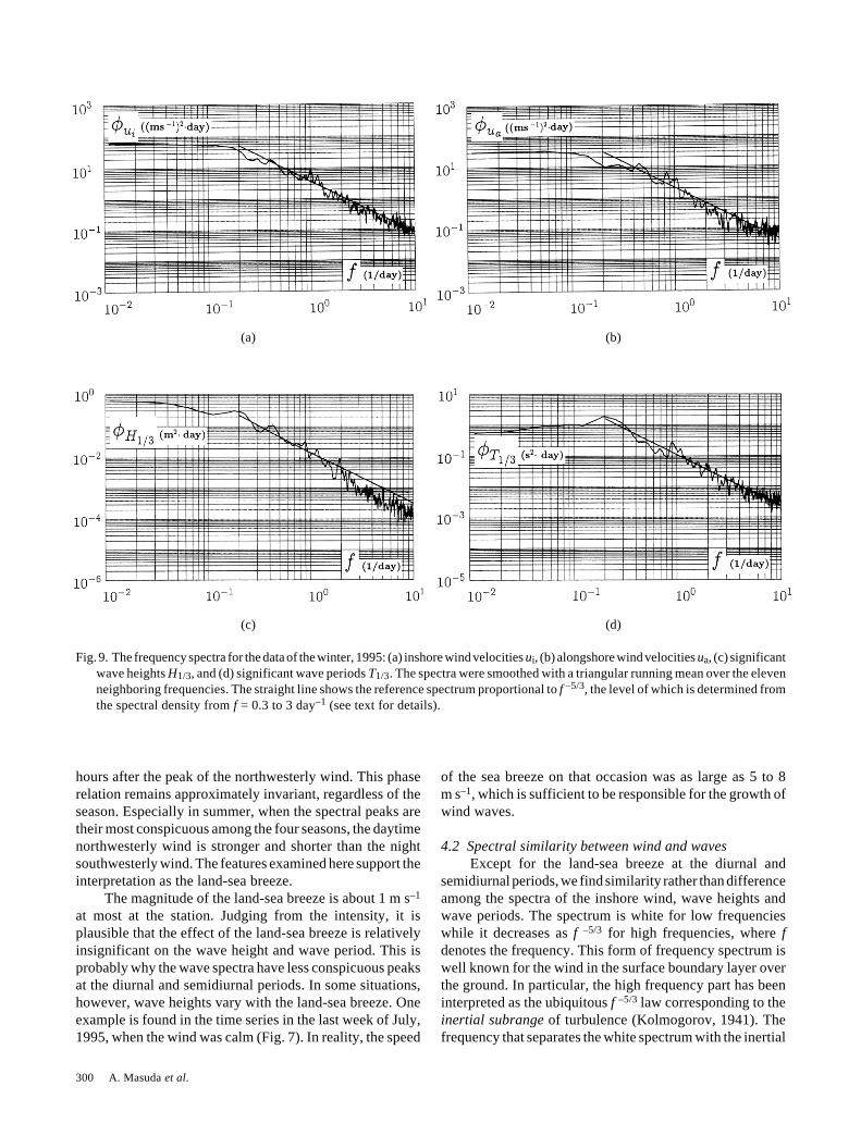
of hourly data for each season. Figures 9 and 10 show thespectra for the summer and winter of 1995: (a) inshore windvelocities ui, (b) alongshore wind velocities ua, (c) signifi-cant wave heights H1/3, and (d) significant wave periodsT1/3, where the spectra were smoothed with a triangularrunning mean over the eleven neighboring frequencies.

4.1 Land-sea breezesA feature that is obvious in the wind spectrum, but

ambiguous in the wave spectrum, is the peaks at the diurnaland semidiurnal periods. The peaks are the most conspicu-ous for ui in summer. It is likely therefore that the peaksrepresent the land-sea breeze. To confirm the inference wedraw stick diagrams of the wind due to the diurnal andsemidiurnal periods for the data of 1995 (Fig. 11). Thosefrequency components of wind blow inshore from the north-west in the daytime around 15 o’clock and offshore from thesoutheast at night around 24 o’clock, which is about ten

(b)(a)

(c) (d)

Fig. 8. Monthly means and error bars of (a) the wind speed U, (b) the wind vector (uE, uN), (c) the significant wave height H1/3, and(d) the significant wave period T1/3. The dotted lines in (a), (c), and (d) indicate the annual mean values.


(a) (b)

(c) (d)

Fig. 9. The frequency spectra for the data of the winter, 1995: (a) inshore wind velocities ui, (b) alongshore wind velocities ua, (c) significantwave heights H1/3, and (d) significant wave periods T1/3. The spectra were smoothed with a triangular running mean over the elevenneighboring frequencies. The straight line shows the reference spectrum proportional to f –5/3, the level of which is determined fromthe spectral density from f = 0.3 to 3 day–1 (see text for details).

hours after the peak of the northwesterly wind. This phaserelation remains approximately invariant, regardless of theseason. Especially in summer, when the spectral peaks aretheir most conspicuous among the four seasons, the daytimenorthwesterly wind is stronger and shorter than the nightsouthwesterly wind. The features examined here support theinterpretation as the land-sea breeze.

The magnitude of the land-sea breeze is about 1 m s–1

at most at the station. Judging from the intensity, it isplausible that the effect of the land-sea breeze is relativelyinsignificant on the wave height and wave period. This isprobably why the wave spectra have less conspicuous peaksat the diurnal and semidiurnal periods. In some situations,however, wave heights vary with the land-sea breeze. Oneexample is found in the time series in the last week of July,1995, when the wind was calm (Fig. 7). In reality, the speed

of the sea breeze on that occasion was as large as 5 to 8m s–1, which is sufficient to be responsible for the growth ofwind waves.

4.2 Spectral similarity between wind and wavesExcept for the land-sea breeze at the diurnal and

semidiurnal periods, we find similarity rather than differenceamong the spectra of the inshore wind, wave heights andwave periods. The spectrum is white for low frequencieswhile it decreases as f –5/3 for high frequencies, where fdenotes the frequency. This form of frequency spectrum iswell known for the wind in the surface boundary layer overthe ground. In particular, the high frequency part has beeninterpreted as the ubiquitous f –5/3 law corresponding to theinertial subrange of turbulence (Kolmogorov, 1941). Thefrequency that separates the white spectrum with the inertial


(a) (b)

(c) (d)

Fig. 10. The same as in Fig. 9 except that the data are for the summer of 1995.

f –5/3 spectrum is found at about 0.2 day–1 in frequency or 5days in period.

It is remarkable, however, that almost the same spectralform is also observed for significant wave heights andsignificant wave periods. So far as we know, this spectralsimilarity has not been discussed in detail for wave proper-ties such as significant wave heights and significant waveperiods. How can we interpret this spectral similarity?Because wind generates surface waves, some associationbetween winds and waves is expected, as we saw in themonthly mean. Take a simple example as follows. Supposethat a linear stochastic system Q is governed by

dQ

dt+ λQ = U t( ), 9( )

where λ–1 is the characteristic time of the response of Q toa random forcing U which has a frequency spectrum ofSU( f ). Then Q has the spectrum SQ( f ) as

SQ f( ) ~SU f( )

λ2 + 2πf( )2 . 10( )

When the response is slow, or the characteristic time λ–1 ismuch larger than the period f –1 in concern, the above for-mula yields

SQ f( ) ~SU f( )2πf( )2 . 11( )

That is, the resulting spectrum SQ( f ) decays faster thanSU( f ). For the opposite case, we have

SQ f( ) ~SU f( )

λ2 . 12( )

In other words, if the response of the system is rapid enough


(a)

we can expect Q to have the same spectral form as theforcing of U.

Such a close spectral similarity between the forcingand the response as in Eq. (12) is not limited to the linearsystem. If there is a direct correspondence between H1/3 and

(b)

(c)

Fig. 11. Stick diagrams of the hourly wind vector due to thecomponents of the diurnal and semidiurnal periods for the dataof (a) winter, (b) summer, and (c) whole one year, respec-tively, 1995. The figures suggest those frequency componentsare interpreted as the land-sea breeze.

(a)

(b)

Fig. 12. The same as in Fig. 9 except that the spectra are for (a)

ui2(t) and (b)

ui t( ) , where ui(t) is the time series observed

in the winter of 1995. For either case the spectral form is thesame as that of ui(t) itself shown in Fig. 9(a).

ui or between T1/3 and ui, the same spectral form may appear.Figure 12 verifies the inference by showing the spectra for

the time series of ui2(t) and

ui t( ) , which were derived by

the ui(t) observed in the winter of 1995. As is anticipated,

both ui2 and

ui have the same spectral form as ui itself,

which is shown in Fig. 9.We must keep in mind, however, that neither wave

heights nor wave periods are directly connected with thelocal wind, as we saw in the scatter diagrams of Subsection3.1. Even at the growing stage, wave heights and waveperiods are not determined solely by the local wind; theyalso depend on the duration and the fetch. Moreover, whenswells are present, the wave properties will be less correlatedwith the local wind. In fact, the correlation was weak inparticular when wind blew offshore (negative inshore wind


velocity), suggesting that the local wind is uncorrelated withwaves propagating inshore as swells. In short, the responseof waves to wind is not straightforward. The large scatter inthe correlation diagrams between the inshore wind velocityand significant wave heights (or wave periods) reflects thiscomplex relation between the local wind and wave proper-ties. Further, a close examination shows that the adequatespectral form of H1/3 valid up to about 8 day–1 is often f –6/

3 or f –7/3, steeper than the inertial form of f –5/3. If within anarrow frequency range (below 2 day–1), however, the f –5/

3 spectral form still seems valid. We again have a questionwhy this subtle difference is observed for H1/3.

The spectral similarity of the inshore wind, wave heights,and wave periods suggests that the spectral properties ofwaves may be ascribed primarily to those of the inshorewind. Then the next question is about the level of thespectrum; if the above supposition is valid, the levels of thefrequency spectra of wave heights and wave periods shouldbe correlated well with those of the inshore wind velocity.To examine the hypothesis, we calculated the representativespectral density at 1 day–1 as an index of the spectral level ofthe inertial range, which is denoted as SL(·) with the argu-ment being the name of the variable. It was obtained byaveraging the spectral density multiplied by f 5/3 over f from0.3 day–1 to 2 day–1. The spectra with this level are drawn bystraight lines in Figs. 9 and 10.

Figure 13 shows the scatter diagrams for the spectrallevels thus determined: (a) SL(H1/3) versus SL(ui), (b)SL(T1/3) versus SL(ui), and (c) SL(H1/3) versus SL(T1/3). Thefigures verify some degree of correlation among the spectrallevels in the inertial range of the inshore wind velocity, waveheights, and wave periods limited within the positive ui

region. The spectral level of H1/3 seems proportional to thatof ui

2, while that of T1/3 is proportional to that of ui2/3, though

the regression may be meaningless at present on account ofthe large scatter. This fact implies that the response to thewind fluctuation is amplified for wave heights and attenu-ated for wave periods, just as we saw in the seasonal cycleof the monthly mean. Also it again suggests that we must becareful when we apply the ordinary fetch relations to thefluctuating wind and waves.

5. Summary and DiscussionThe sea surface wind and wind waves were analyzed to

yield their fundamental statistics based on the hourly datafrom 1990 to 1997 obtained at an observation tower offTsuyazaki, Fukuoka, in the Eastern Tsuhima Strait.

First, fundamental statistics were analyzed. The annualmean was calculated for wind speeds U, wind vectors (uE, uN),significant wave heights H1/3, and significant wave periodsT1/3. Also yearly maximum values were determined for the12 minute maximum wind speed and 12 minute maximumwave height. After that, correlation was investigated amongui, H1/3, and T1/3. Although the scatter was rather large, some

(a)

(b)

(c)

Fig. 13. Scatter diagrams of spectral levels SL of the inertial rangefor the four seasons of 1990 to 1997: (a) SL(H1/3) versus SL(ui),(b) SL(T1/3) versus SL(ui), and (c) SL(H1/3) versus SL(T1/3). Thestraight line added in the figure shows a reference slope of thescaling law: (a) SL(H1/3) ∝ SL2(ui), (b) SL(T1/3) ∝ SL2/3(ui), and(c) SL(H1/3) ∝ SL3(T1/3).


degree of correlation was found among them, especially forthe data of positive ui in winter. By fitting the data to scalinglaws, the effective fetch was inferred to be 50 km or longer.The estimated fetch seems reasonable, since Iki Is. is 60 kmwest and Tsushima Is. is 110 km northwest of the station.

The scatter diagram of H1/3 against T1/3 revealed thatmost H1/3 data are limited from above by a quadratic curveof T1/3. That is, the data off Tsuyazaki have an upper boundof wave steepness, regardless of the season or the windspeed. The reason for this is not clear. This upper bound doesnot apply to wind waves in the wind flume, at least. It isworthwhile examining whether this upper bound is appli-cable to other sources of wave data and to elucidate thephysics responsible for this upper bound of wave steepness.

Then the seasonal variation was examined. Monthlymean wind speeds attain their peaks in January, when thenorthwesterly monsoon prevails in East Asia. The monthlymean wind blows most weakly in June (not July). Monthlymean significant wave heights H1/3 and wave periods T1/3

have similar sinusoidal seasonal cycles as the monthly meanwind speed U; the wind vector rotates clockwise from De-cember to March and anticlockwise in the remaining periodof the year. The association between wind and waves isplausible, because strong wind develops high and longwaves. Moreover the winter monsoon is preferable for thegrowth of waves observed at the station off Tsuyazaki; thenorthwesterly wind allows a longer fetch, favorable for thedevelopment of waves. The variability of the seasonal cyclerelative to the annual mean is maximum for wave heights,moderate for wind speeds, and minimum for wave periods.This fact suggests that the response of wave heights to windsis enhanced, whereas that of wave periods is reduced.

For periods shorter than a month, the variability wasinvestigated through spectral analysis. The wind spectrumhas peaks at the diurnal and semidiurnal periods, thoughthey are ambiguous in the spectra of H1/3 or T1/3. From a fewproperties analyzed, they were interpreted well as the land-sea breeze. Although the wind speed due to these spectralcomponents were 1 m s–1 at most, sea breezes of 5 to 8m s–1 were confirmed to blow in some situations, so thatland-sea breezes often play a significant role in the fluctua-tion of wave heights and wave periods.

One notable finding is that both significant wave heightsand wave periods have almost the same spectral form as theinshore wind velocity ui: it is white for periods longer than5 days and decays as f –5/3 for shorter periods. Although thisspectral shape is familiar in boundary-layer meteorology,the same spectral form is remarkable with respect to sig-nificant wave heights and significant wave periods, whichdepend not only on the local wind but also on the windduration or the fetch even at the developing stage of windwaves. The local wind loses an intimate relationship withwaves coexisting with swells. In fact the observed correla-tion was poor when the wind blows offshore. It was worse

between significant wave periods and inshore wind veloci-ties. Moreover, a close examination revealed that significantwave heights H1/3 tend to have a spectrum that decaysslightly faster than f –5/3, though we do not know why.

In parallel to the spectral form, the correlation betweenthe spectral levels in the inertial frequency range of theinshore wind velocity was compared with those of thesignificant wave height (or the significant wave period). Thelatter spectral level appeared to increase with the formerspectral level. The scatter was so large that it was difficult toderive simple relations between wave heights (periods) andthe inshore wind velocity. At least, however, the spectrallevel of wave heights increases with that of the inshore windspeed more rapidly than that of wave periods. This agreeswith the difference in the seasonal variability relative to theannual mean among the wind speed, wave heights, and waveperiods. That is, wave heights respond to the variability ofthe wind speed sensitively, whereas wave periods in a lesssensitive way.

The similarity of the spectral form is worthy of furtherinvestigation. It is not straightforward to explain the prop-erties revealed here, although some explanation has beenattempted in the paper. We need further evidence of thisform of frequency spectrum for similar data of differentlocations. We also have to answer to the question why thespectrum H1/3 in the inertial range decays more rapidly thanthose of ui, ua, or T1/3. Are these phenomena common toother locations or peculiar to the station off Tsuyazaki? It isnecessary to accumulate similar data to be compared withour data representative of the maritime condition of theEastern Tsushima Strait. One of the goals of the Japan SeaProject of the RIAM is to establish the climatology of the seasurface wind and wind waves over and along the coast of theJapan Sea, for oceanographic, engineering, fishery, andsocial purposes.

The first objective of the study was to prepare thefundamental statistics on climatology of the wind and wavesobserved at a representative ocean station in the EasternTsushima Strait. During the study, however, intriguingphenomena were found such as a uniform upper bound of thesteepness of significant waves off Tsuyazaki or the spectralsimilarity among the inshore wind, wave heights, and waveperiods. In addition, tide levels, water temperature, and soon are being accumulated at the Tsuyazaki Station. Thesedata are expected to reveal other kinds of oceanographicvariability of the Eastern Tsushima Strait. All of these areleft for future analysis and dynamical research.

AcknowledgementsThe study was partially supported by Grant-in-Aid for

Scientific Research from the Ministry of Education andCulture, Japan, as well as by a fund for the CooperativeStudy from the Research Institute for Applied Mechanics,Kyushu University. We would like to thank the committee


of the Tsuyazaki Maritime Laboratory for their cooperation.We also appreciate Mr. Abe for his work in maintaining theTsuyazaki Sea Observation Tower. Thanks are due to Mr.Yada for his assistance in the data analysis.

ReferencesDonelan, M. A. (1993): On the dependence of sea surface rough-

ness on wave development. J. Phys. Oceanogr., 23, 2143–2149.Hasselmann, K., T. P. Barnett, E. Bouws, H. Carlson, D. E.

Cartwright, K. Enke, J. A. Ewing, H. Gienapp, D. E.Hasselmann, P. Kruseman, A. Meerburg, P. Müller, D. J.Olbers, K. Richter, W. Sell and H. Walden (1973): Measure-ments of wind-wave growth and swell decay during the JointNorth Sea Wave Project (JONSWAP). Dtsch. Hydrogr. Z.,Suppl. A.8, No. 12, 1-95.

Koga, M. (1984): Characteristics of a breaking wind-wave field inthe light of the individual wind-wave concept. J. Oceanogr.Soc. Japan, 40, 105–114.

Kolmogorov, A. N. (1941): The local structure of turbulence inincompressible viscous fluid for very large Reynolds number.Dokl. Akad. Nauk SSSR, 30, 301–305.

Komen, G., P. A. E. M. Janssen, V. Makin and W. Oost (1998): Onthe sea state dependence of the Charnock parameter. GlobalAtmosphere and Ocean System, 5, 367–388.

Kusaba, T. and A. Masuda (1989): Wind-wave spectra based onthe hypothesis of local equilibrium. J. Oceanogr. Soc. Japan,45, 45–64.

Longuet-Higgins, M. S. (1952): On the statistical distribution ofthe height of sea waves. J. Mar. Res., 11, 245–266.

Marubayashi, K., M. Ishibashi, H. Honji and H. Mitsuyasu (1989):

A telemeter system for oceanographic observation. Rep. Res.Inst. Appl. Mech. Kyushu Univ., 68, 525–544 (in Japanese).

Masuda, A. (1998): A research project for the air-sea interactionand the oceanic and atmospheric variability in the Japan Sea.Kaiyo Monthly, 30, No. 8, 447–455 (in Japanese).

Masuda, A. and T. Kusaba (1987): On the local equilibrium ofwinds and wind-waves in relation to surface drag. J. Oceanogr.Soc. Japan, 43, 28–36.

Michell, J. H. (1893): On the highest waves in water. Phil. Mag.,36(5), 430–437.

Mitsuyasu, H. (1968): On the growth of the spectrum of wind-generated waves I. Rep. Res. Inst. Appl. Mech., Kyushu Univ.,16, 459–465.

Mitsuyasu, H. (1969): On the growth of the spectrum of wind-generated waves II. Rep. Res. Inst. Appl. Mech., Kyushu Univ.,17, 235–243.

Smith, S. D., R. J. Anderson, W. A. Oost, C. Kraan, N. Maat, J.DeCosmo, K. B. Katsaros, K. L. Davidson, K. Bumke, L.Hasse and H. M. Chadwick (1992): Sea surface wind stressand drag coefficients: The HEXOS results. Boudary-LayerMet., 60, 109–142.

Toba, Y. (1972): Local balance in the air-sea boundary processes.I. On the growth process of wind waves. J. Oceanogr. Soc.Japan, 28, 109–120.

Toba, Y., N. Iida, H. Kawamura, N. Ebuchi and I. S. F. Jones(1990): Wave dependence of sea-surface wind stress. J. Phys.Oceanogr., 20, 705–721.

Wilson, B. W. (1965): Numerical prediction of ocean waves in theNorth Atlantic for December, 1959. Dtsch. Hydrogr. Z., 18,114–130.

statistics of wind and waves off tsuyazaki, fukuoka, in ... · akira masuda, tadao kusaba, kenji...

Documents