stochastic guide for a time-delay object in a positional differential game

ISSN 0081-5438, Proceedings of the Steklov Institute of Mathematics, 2012, Vol. 277, Suppl. 1, pp. S145–S151.c© Pleiades Publishing, Ltd., 2012.Original Russian Text c© N.N. Krasovskii, A.N. Kotel’nikova, 2011,published in Trudy Instituta Matematiki i Mekhaniki UrO RAN, 2011, Vol. 17, No. 2.

Stochastic Guide for a Time-Delay Object

in a Positional Differential Game

N. N. Krasovskii†1 and A. N. Kotel’nikova1

Received February 1, 2011

Abstract—A positional differential time-optimal game is considered for a conflict-controlledtime-delay object. Minimax and maximin feedback controls are constructed within a schemethat includes an intermediate model object described by an ordinary differential equation anda stochastic guide described by the Ito differential equation. The motion of the guide is basedon the real-time solution of a sequence of auxiliary boundary value problems for a parabolicequation with a degenerate diffusion term.Keywords: time-delay object, minimax–maximin time to the encounter, stochastic guide.

DOI: 10.1134/S0081543812050148

INTRODUCTION

For a conflict-controlled object described by a time-delay equation, a differential game onthe minimax–maximin time to the encounter with a given set M inside a given set N in thephase x-space of this object [1–3] is considered. Approximative minimax and maximin feedbackcontrols are built based on stochastic guides included in the loop. The connection between theinitial x-object described by a time-delay equation and a stochastic w-guide described by theIto differential equation is closed by an intermediate approximation model y-object described byan ordinary differential equation. The motions of the guide are formed by solving in real timea sequence of auxiliary approximation boundary value problems for parabolic equations with adegenerate diffusion term. This is done by the method developed in [4–6] for initial x-objectsdescribed by ordinary differential equations. In the proposed method of building controls for theinitial time-delay x-object, we use the theorem on the proximity of motions of the x-object andthe approximating ordinary y-object for sufficiently large dimensions of the y-object. A similarapproximation of an x-object by a y-object was used in many studies of stability and controlproblems for time-delay systems (see, e.g., [7–11]). The proposed generation of controls with astochastic guide for time-delay systems is based on the theory of parabolic equations [12].

1. DIFFERENTIAL APPROACH–EVASION GAME FOR A TIME-DELAY SYSTEM

Consider the equation of motion of a controlled x-object

x[t] = f(t, x[t], x[t − h], u, v), t0 ≤ t ≤ τ, |x| < ∞. (1.1)1Institute of Mathematics and Mechanics, Ural Branch of the Russian Academy of Sciences, ul. S. Kovalevskoi 16,Yekaterinburg, 620990 Russiaemail: [email protected]

S145

S146 KRASOVSKII, KOTEL’NIKOVA

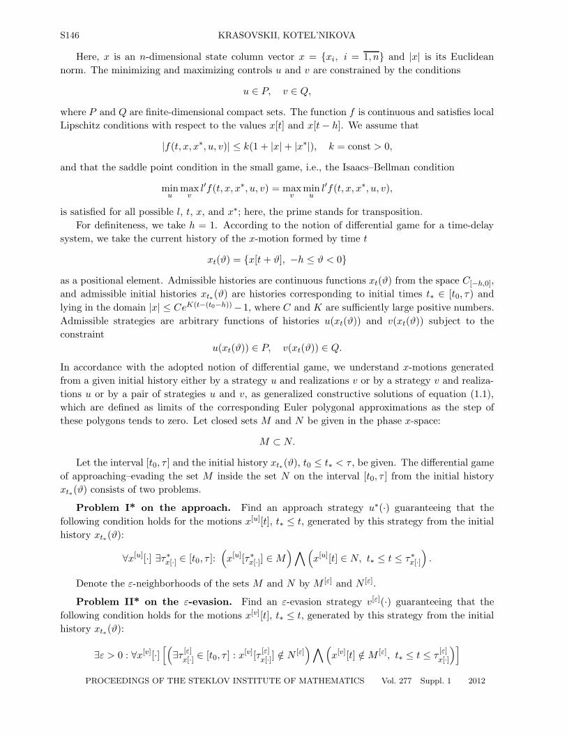
Here, x is an n-dimensional state column vector x = {xi, i = 1, n} and |x| is its Euclideannorm. The minimizing and maximizing controls u and v are constrained by the conditions

u ∈ P, v ∈ Q,

where P and Q are finite-dimensional compact sets. The function f is continuous and satisfies localLipschitz conditions with respect to the values x[t] and x[t − h]. We assume that

|f(t, x, x∗, u, v)| ≤ k(1 + |x| + |x∗|), k = const > 0,

and that the saddle point condition in the small game, i.e., the Isaacs–Bellman condition

minu

maxv

l′f(t, x, x∗, u, v) = maxv

minu

l′f(t, x, x∗, u, v),

is satisfied for all possible l, t, x, and x∗; here, the prime stands for transposition.For definiteness, we take h = 1. According to the notion of differential game for a time-delay

system, we take the current history of the x-motion formed by time t

xt(ϑ) = {x[t + ϑ], −h ≤ ϑ < 0}

as a positional element. Admissible histories are continuous functions xt(ϑ) from the space C[−h,0],and admissible initial histories xt∗(ϑ) are histories corresponding to initial times t∗ ∈ [t0, τ) andlying in the domain |x| ≤ CeK(t−(t0−h)) −1, where C and K are sufficiently large positive numbers.Admissible strategies are arbitrary functions of histories u(xt(ϑ)) and v(xt(ϑ)) subject to theconstraint

u(xt(ϑ)) ∈ P, v(xt(ϑ)) ∈ Q.

In accordance with the adopted notion of differential game, we understand x-motions generatedfrom a given initial history either by a strategy u and realizations v or by a strategy v and realiza-tions u or by a pair of strategies u and v, as generalized constructive solutions of equation (1.1),which are defined as limits of the corresponding Euler polygonal approximations as the step ofthese polygons tends to zero. Let closed sets M and N be given in the phase x-space:

M ⊂ N.

Let the interval [t0, τ ] and the initial history xt∗(ϑ), t0 ≤ t∗ < τ , be given. The differential gameof approaching–evading the set M inside the set N on the interval [t0, τ ] from the initial historyxt∗(ϑ) consists of two problems.

Problem I* on the approach. Find an approach strategy u∗(·) guaranteeing that thefollowing condition holds for the motions x[u][t], t∗ ≤ t, generated by this strategy from the initialhistory xt∗(ϑ):

∀x[u][·] ∃τ∗x[·] ∈ [t0, τ ]:

(x[u][τ∗

x[·]] ∈ M) ∧(

x[u][t] ∈ N, t∗ ≤ t ≤ τ∗x[·]

).

Denote the ε-neighborhoods of the sets M and N by M [ε] and N [ε].

Problem II* on the ε-evasion. Find an ε-evasion strategy v[ε](·) guaranteeing that thefollowing condition holds for the motions x[v][t], t∗ ≤ t, generated by this strategy from the initialhistory xt∗(ϑ):

∃ε > 0 : ∀x[v][·][(

∃τ[ε]x[·] ∈ [t0, τ ] : x[v][τ [ε]

x[·]] /∈ N [ε])∧(

x[v][t] /∈ M [ε], t∗ ≤ t ≤ τ[ε]x[·]

)]

PROCEEDINGS OF THE STEKLOV INSTITUTE OF MATHEMATICS Vol. 277 Suppl. 1 2012

STOCHASTIC GUIDE FOR A TIME-DELAY OBJECT S147

∨[(x[v][t] ∈ N [ε], t∗ ≤ t ≤ τ

) ∧(x[v][t] /∈ M [ε], t∗ ≤ t ≤ τ

)].

The following theorem of alternatives [2] is valid.

Theorem 1. For the interval [t0, τ ] and initial history xt∗(ϑ), t0 ≤ t∗ < τ , one and only oneof the two assertions is true: either the problem on the approach is solvable or the problem on theε-evasion is solvable.

Given the initial history xt∗(ϑ), assume that there exists an interval [t0, τ ] for which Problem I*on the approach is solvable for this initial history. Then, the theorem from [1, 3] is valid. Thereexists a smallest value τ0, t∗ ≤ τ0 ≤ τ , for which the approach problem is solvable. Moreover, forany value τ∗, t∗ ≤ τ∗ < τ0, there exists ε∗ > 0 such that, for the given initial history, Problem II*on the ε-evasion is solvable for ε = ε∗.

These theorems are descriptive.In the present paper, we give a constructive method of forming approximative minimax and

maximin controls for the time-delay object under consideration. This is a development (for time-delay systems) of the method of forming minimax and maximin controls based on a stochastic guidefor objects described by ordinary differential equations [5, 6]. Here, an essential role is played bythe approximation of the time-delay object by an appropriate model object described by a highlymultidimensional ordinary differential equation.

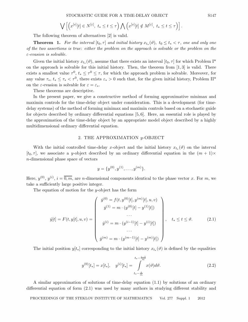
2. THE APPROXIMATION y-OBJECT

With the initial controlled time-delay x-object and the initial history xt∗(ϑ) on the interval[t0, τ ], we associate a y-object described by an ordinary differential equation in the (m + 1)×n-dimensional phase space of vectors

y = {y(0), y(1), . . . , y(m)}.

Here, y(0), y(i), i = 0,m, are n-dimensional components identical to the phase vector x. For m, wetake a sufficiently large positive integer.

The equation of motion for the y-object has the form

y[t] = F (t, y[t], u, v) =

⎛⎜⎜⎜⎜⎜⎜⎜⎜⎜⎜⎜⎝

y(0) = f(t, y(0)[t], y(m)[t], u, v)

y(1) = m · (y(0)[t] − y(1)[t])

· · ·y(i) = m · (y(i−1)[t] − y(i)[t])

· · ·y(m) = m · (y(m−1)[t] − y(m)[t])

⎞⎟⎟⎟⎟⎟⎟⎟⎟⎟⎟⎟⎠

, t∗ ≤ t ≤ ϑ. (2.1)

The initial position y[t∗] corresponding to the initial history xt∗(ϑ) is defined by the equalities

y(0)[t∗] = x[t∗], y(i)[t∗] =

t∗− i−1m∫

t∗− im

x(ϑ)dϑ. (2.2)

A similar approximation of solutions of time-delay equation (1.1) by solutions of an ordinarydifferential equation of form (2.1) was used by many authors in studying different stability and



control problems for time-delay systems (see, for example, [7–11]). The justification of suchapproximation for the problem of stabilizing a controlled time-delay system was given in [9]. Forthe initial history xt∗(ϑ) and initial position y[t∗] (2.2), we will consider approximative solutionsof equations (1.1) and (2.1), i.e., Euler polygons x[t] and y[t], which are solutions of the followingfinite difference equations. In the case of minimax control, we write

x[t] = f(τj , x[τj], x[τj − 1], u[x][τj], v[t]

),

y[t] = F(τj, y[τj ], u[t], v[y][τj ]

),

τj ≤ t < τj+1, j = 1, 2 . . . , τ1 = t∗,

τj+1 − τj ≤ δ, δ > 0.

Here, v[t] and u[t] are arbitrary admissible piecewise continuous realizations

u[t] ∈ P, v[t] ∈ Q, (2.3)

and the controls u[x][τj ] and v[y][τj] are chosen from the conditions

u[x][τj ] ∈ arg maxu

minv

l′[τj ]f(τj, x[τj ], x[τj − h], u, v

),

(2.4)

v[y][τj] ∈ arg minv

maxu

l′[τj]f(τj, y

(0)[τj ], y(m)[τj], u, v).

In the case of maximin control, we write

x[t] = f(τj , x[τj], x[τj − 1], u[t], v[x][τj]

), (2.5)

y[t] = F(τj, y[τj ], u[y][τj ], v[t]

). (2.6)

Here, v[t] and u[t] are arbitrary admissible piecewise continuous realizations satisfying condi-tions (2.3), while the controls u[y][τj ] and v[x][τj] are chosen from the conditions

v[x][τj] ∈ arg maxv

minu

l′[τj]f(τj , x[τj], x[τj − 1], u, v

), (2.7)

u[y][τj ] ∈ arg minu

maxv

l′[τj ]f(τj, y

(0)[τj], y(m)[τj ], u, v). (2.8)

Here, in (2.5)–(2.8), we havel[τj ] = y(0)[τj ] − x[τj ].

Theorem 2. For the interval [t0, τ ] and chosen initial history xt∗(ϑ) and initial position y[t∗](see (2.2)), for any prescribed ε > 0, there exists a sufficiently large number m∗ and a sufficientlysmall value δ(m) > 0 such that the inequality

|x[t] − y(0)[t]| < ε, t∗ ≤ t ≤ τ,

holds for m > m∗ and δ < δ(m).

Since the proof of this proximity theorem involves a considerable number of calculations, whichexceed the volume of this paper, we omit the proof of Theorem 2. The proof is carried out by thescheme of the proof of a similar proximity theorem from [9] and differs in details related to thespecific form of the equations and the nature of the problems under consideration.



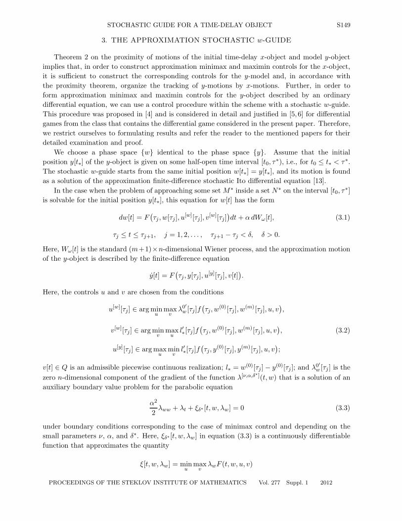
3. THE APPROXIMATION STOCHASTIC w-GUIDE

Theorem 2 on the proximity of motions of the initial time-delay x-object and model y-objectimplies that, in order to construct approximation minimax and maximin controls for the x-object,it is sufficient to construct the corresponding controls for the y-model and, in accordance withthe proximity theorem, organize the tracking of y-motions by x-motions. Further, in order toform approximation minimax and maximin controls for the y-object described by an ordinarydifferential equation, we can use a control procedure within the scheme with a stochastic w-guide.This procedure was proposed in [4] and is considered in detail and justified in [5, 6] for differentialgames from the class that contains the differential game considered in the present paper. Therefore,we restrict ourselves to formulating results and refer the reader to the mentioned papers for theirdetailed examination and proof.

We choose a phase space {w} identical to the phase space {y}. Assume that the initialposition y[t∗] of the y-object is given on some half-open time interval [t0, τ∗), i.e., for t0 ≤ t∗ < τ∗.The stochastic w-guide starts from the same initial position w[t∗] = y[t∗], and its motion is foundas a solution of the approximation finite-difference stochastic Ito differential equation [13].

In the case when the problem of approaching some set M∗ inside a set N∗ on the interval [t0, τ∗]is solvable for the initial position y[t∗], this equation for w[t] has the form

dw[t] = F(τj , w[τj ], u[w][τj], v[w][τj]

)dt + αdWω[t], (3.1)

τj ≤ t ≤ τj+1, j = 1, 2, . . . , τj+1 − τj < δ, δ > 0.

Here, Wω[t] is the standard (m+1)×n-dimensional Wiener process, and the approximation motionof the y-object is described by the finite-difference equation

y[t] = F(τj, y[τj ], u[y][τj ], v[t]

).

Here, the controls u and v are chosen from the conditions

u[w][τj] ∈ arg minu

maxv

λ0′w [τj ]f

(τj, w

(0)[τj], w(m)[τj], u, v),

v[w][τj] ∈ arg minv

maxu

l′∗[τj]f(τj, w

(0)[τj ], w(m)[τj ], u, v), (3.2)

u[y][τj] ∈ arg maxu

minv

l′∗[τj ]f(τj, y

(0)[τj], y(m)[τj ], u, v);

v[t] ∈ Q is an admissible piecewise continuous realization; l∗ = w(0)[τj ] − y(0)[τj ]; and λ0′w [τj ] is the

zero n-dimensional component of the gradient of the function λ[ν,α,δ∗](t, w) that is a solution of anauxiliary boundary value problem for the parabolic equation

α2

2λww + λt + ξδ∗ [t, w, λw] = 0 (3.3)

under boundary conditions corresponding to the case of minimax control and depending on thesmall parameters ν, α, and δ∗. Here, ξδ∗ [t, w, λw] in equation (3.3) is a continuously differentiablefunction that approximates the quantity

ξ[t, w, λw] = minu

maxv

λwF (t, w, u, v)



in a sufficiently large domain of the space {t, w} and for |λw| < ∞ so that the following conditionholds:

ξδ∗ [t, w, λw] − ξ[t, w, λw] < δ∗.

In the case when the problem of the ε-evasion from the set M inside the set N on theinterval [t0, τ∗] is solvable for the initial position y[t∗] and some fixed ε∗ > 0, the equation forthe w-guide has the same form (3.1), but the motion of the y-object takes the form

y[t] = F (τj , y[τj ], u[t], v[y][τj ]);

the controls u and v are found from the conditions

u[w][τj] ∈ arg minu

maxv

l′∗[τj ]f(τj, w

(0)[τj ], w(m)[τj], u, v),

v[w][τj ] ∈ arg maxv

minu

λ0′w [τj ]f

(τj, w

(0)[τj ], w(m)[τj ], u, v), (3.4)

v[y][τj] ∈ arg maxv

minu

l′∗[τj ]f(τj, y(0)[τj], y(m)[τj ], u, v),

where u[t] ∈ P is an admissible piecewise continuous realization. Here, λ0′w [τj ] is the zero n-

dimensional component of the gradient of the function λ[ν,α,δ∗](t, w) that is a solution of an auxiliaryboundary value problem for the parabolic equation

α2

2λww + λt + ξδ∗ [t, w, λw] = 0

under boundary conditions corresponding to the case of maximin control and depending on thesmall parameters ν, α, and δ∗.

Assertion 1. In the case of minimax control, for any ε > 0 and β < 1, one can specify smallvalues of ν, α, δ∗, and δ such that, for the y-motion, the encounter of y(0)[t] with the ε-neighborhoodM∗(ε) inside the ε-neighborhood N∗(ε) on the interval [t0, τ∗] will be provided with probability P notless than β.

Assertion 2. In the case of maximin control, for any ε < ε∗ and β < 1, one can specify smallvalues of ν, α, δ∗, and δ such that, for the y-motion, the evasion of y(0)[t] from the ε-neighborhoodM∗(ε) inside the ε-neighborhood N∗(ε) on the interval [t0, τ∗] will be provided with probability P notless than β.

4. MINIMAX APPROXIMATION CONTROL

OF THE INITIAL TIME-DELAY x-OBJECT

In the minimax case, we close the system consisting of the initial time-delay x-object, theintermediate y-model described by an ordinary differential equation, and the stochastic w-guidedescribed by the Ito differential equation by assuming in the theorem on the proximity of themotions x and y that the control u[t] for the y-model is assigned by the rule specified in (3.2) andthe control v[t] for the y-model from Section 3 is assigned by rule (2.4) specified in the proximitytheorem for the motions x and y. Then, the following statement is valid.

Theorem 3. Assume that Problem I* on the approach of the motion x[t] to the set M insidethe set N on the interval [t0, τ∗] is solvable for the initial history xt∗(ϑ). Then, for any ε > 0 andβ < 1, one can specify a large value m and small values δ(m) and parameters ν, α, and δ∗ suchthat the encounter of the motion x[t] with the ε-neighborhood M (ε) inside the ε-neighborhood N (ε)

will be guaranteed with probability not less than β.



5. MAXIMIN APPROXIMATION CONTROL

OF THE INITIAL TIME-DELAY X-OBJECT

In the maximin case, we close the system consisting of the initial time-delay x-object, theintermediate y-model described by an ordinary differential equation, and the stochastic w-guidedescribed by the Ito differential equation by assuming in the theorem on the proximity of themotions x and y that the control v[t] for the y-model is assigned by the rule specified in (3.4) andthe control u[t] for the y-model from Section 3 is assigned by rule (2.8) specified in the proximitytheorem for the motions x and y. Then, the following statement is valid.

Theorem 4. Assume that Problem II* on the ε-evasion of the motion x[t] from the set M

inside the set N on the interval [t0, τ∗] is solvable for fixed ε = ε∗ and the initial history xt∗(ϑ).Then, for any 0 < ε < ε∗ and β < 1, one can specify a large value m and small values δ(m) andparameters ν, α, and δ∗ such that the ε-evasion of the motion x[t] from the ε-neighborhood M (ε)

inside the ε-neighborhood N (ε) on the interval [t0, τ∗] will be guaranteed with probability not lessthan β.

The described constructions of the control with a stochastic guide based on solving auxiliaryapproximation boundary value problems for the parabolic equations under consideration are real-izable for a rather general case of the sets M and N in accordance with the classical methods ofthe theory of parabolic equations [12]. However, the practical realization of this method is hardlypossible because of the immense number of calculations that must be implemented in real time.

It is typical for the considered approximation of a differential game in a time-delay system thatthe conditions imposed on the controls in the x-object, y-model, and w-guide are similar to theextremal shift conditions in a time-delay system, which were established and used in [1–3], and tothe extremal shift conditions in ordinary and a stochastic systems, which were used in [5, 6].

ACKNOWLEDGMENTS

This work was supported by the Ural Branch of the Russian Academy of Sciences (project no. 09-P-1-1015) within the Program of the Presidium of the Russian Academy of Sciences “MathematicalTheory of Control” and by the Russian Foundation for Basic Research (project no. 09-01-00313).

REFERENCES1. Yu. S. Osipov, Dokl. Akad. Nauk SSSR 196 (4), 779 (1971).

2. Yu. S. Osipov, Dokl. Akad. Nauk SSSR 197 (5), 1022 (1971).

3. Yu. S. Osipov, J. Appl. Math. Mech. 35 (2), 262 (1971).

4. N. N. Krasovskii, Dokl. Akad. Nauk SSSR 237 (5), 1020 (1977).

5. N. N. Krasovskii and A. N. Kotel’nikova, Autom. Remote Control 72 (2), 305 (2011).

6. N. N. Krasovskii and A. N. Kotel’nikova, Proc. Steklov Inst. Math. 268 (1), 161 (2010).

7. M. E. Salukvadze, Automat. Remote Control 23, 1495 (1962).

8. Yu. M. Repin and V. E. Tret’yakov, Avtomat. i Telemekh. 24 (6), 738 (1963).

9. N. N. Krasovskii, J. Appl. Math. Mech. 28 (4), 876 (1964).

10. Yu. M. Repin, J. Appl. Math. Mech. 29 (2), 254 (1965).

11. A. B. Kurzhanskii, Differents. Uravneniya 3 (12), 2094 (1967).

12. O. A. Ladyzhenskaya, V. A. Solonnikov, and N. N. Ural’tseva, Linear and Quasilinear Equations of ParabolicType (Nauka, Moscow, 1967; Amer. Math. Soc., Providence, 1968).

13. R. Sh. Liptser and A. N. Shiryaev, Statistics of Random Processes (Nauka, Moscow, 1974) [in Russian].

Translated by I. Tselishcheva


stochastic guide for a time-delay object in a positional differential game

Documents