study on heterogeneity of oxide films formed on ... · title study on heterogeneity of oxide films...
TRANSCRIPT

Instructions for use
Title Study on Heterogeneity of Oxide Films Formed on Polycrystalline Iron
Author(s) 高畠, 勇
Issue Date 2017-03-23
DOI 10.14943/doctoral.k12795
Doc URL http://hdl.handle.net/2115/67741
Type theses (doctoral)
File Information Yu_Takabatake.pdf
Hokkaido University Collection of Scholarly and Academic Papers : HUSCAP
Study on
Heterogeneity of Oxide Films
Formed on Polycrystalline Iron
多結晶鉄上に形成する酸化物皮膜の
不均一性に関する研究
Yu Takabatake
Graduate School of Chemical Sciences and Engineering
Hokkaido University
March 2017
Table of contents
Chapter 1 Introduction
1.1. Corrosion of metals . . . . . . . . . . . . . . . . . . . . . . . . . . . . . . . . . . . . . . . . . . . . . . . . . . . 1
1.1.1. Significance of corrosion study . . . . . . . . . . . . . . . . . . . . . . . . . . . . . . . . . . . . . . . . . . 1
1.1.2. Anisotropic corrosion . . . . . . . . . . . . . . . . . . . . . . . . . . . . . . . . . . . . . . . . . . . . . . . . . 2
1.2. Iron . . . . . . . . . . . . . . . . . . . . . . . . . . . . . . . . . . . . . . . . . . . . . . . . . . . . . . . . . . . . . . . 3
1.2.1. General characteristics . . . . . . . . . . . . . . . . . . . . . . . . . . . . . . . . . . . . . . . . . . . . . . . . 3
1.2.2. Corrosion behavior . . . . . . . . . . . . . . . . . . . . . . . . . . . . . . . . . . . . . . . . . . . . . . . . . . . 4
1.2.3 Passive film . . . . . . . . . . . . . . . . . . . . . . . . . . . . . . . . . . . . . . . . . . . . . . . . . . . . . . . . . 7
1.3. Analytical techniques . . . . . . . . . . . . . . . . . . . . . . . . . . . . . . . . . . . . . . . . . . . . . . . . . 15
1.3.1 Vacuum analysis . . . . . . . . . . . . . . . . . . . . . . . . . . . . . . . . . . . . . . . . . . . . . . . . . . . . . 15
1.3.2 Optical measurements . . . . . . . . . . . . . . . . . . . . . . . . . . . . . . . . . . . . . . . . . . . . . . . . . 17
1.3.3. Micro-electrochemical measurement methods . . . . . . . . . . . . . . . . . . . . . . . . . . . . . . 17
1.4. Previous study on orientation-dependent corrosion of iron . . . . . . . . . . . . . . . . . . . . 19
1.5. Purpose of this dissertation . . . . . . . . . . . . . . . . . . . . . . . . . . . . . . . . . . . . . . . . . . . . . 20
References . . . . . . . . . . . . . . . . . . . . . . . . . . . . . . . . . . . . . . . . . . . . . . . . . . . . . . . . . . . . . . . . . 23
Chapter 2 Experimental techniques and setups
2.1. Sample preparation . . . . . . . . . . . . . . . . . . . . . . . . . . . . . . . . . . . . . . . . . . . . . . . . . . . 39
2.1.1. Grain coarsening . . . . . . . . . . . . . . . . . . . . . . . . . . . . . . . . . . . . . . . . . . . . . . . . . . . . . 39
2.1.2. Surface polishing . . . . . . . . . . . . . . . . . . . . . . . . . . . . . . . . . . . . . . . . . . . . . . . . . . . . . 39
2.1.3. Identification of surface crystallographic orientation . . . . . . . . . . . . . . . . . . . . . . . . . 40
2.2. Electrochemical measurements with micro-capillary cell . . . . . . . . . . . . . . . . . . . . . 41
2.2.1. Fabrication of micro-capillary . . . . . . . . . . . . . . . . . . . . . . . . . . . . . . . . . . . . . . . . . . . 41
2.2.2. Micro-reference electrode . . . . . . . . . . . . . . . . . . . . . . . . . . . . . . . . . . . . . . . . . . . . . . 42
2.2.3. Setup of micro-capillary cell . . . . . . . . . . . . . . . . . . . . . . . . . . . . . . . . . . . . . . . . . . . 42
2.2.4. Measurement procedure . . . . . . . . . . . . . . . . . . . . . . . . . . . . . . . . . . . . . . . . . . . . . . . 43
2.3. Two-dimensional ellipsometry . . . . . . . . . . . . . . . . . . . . . . . . . . . . . . . . . . . . . . . . . . 44
2.3.1. Principle of ellipsometry . . . . . . . . . . . . . . . . . . . . . . . . . . . . . . . . . . . . . . . . . . . . . . . 44
2.3.2. Two-dimensional ellipsometry measurement . . . . . . . . . . . . . . . . . . . . . . . . . . . . . . . 47
2.3.3. Setup of electrochemical cell for in situ 2D ellipsometry . . . . . . . . . . . . . . . . . . . . . 48
References . . . . . . . . . . . . . . . . . . . . . . . . . . . . . . . . . . . . . . . . . . . . . . . . . . . . . . . . . . . . . . . . . 48
Chapter 3 Grain-dependent oxidation behavior in sulfuric acid
measured by micro-capillary cell
3.1. Introduction . . . . . . . . . . . . . . . . . . . . . . . . . . . . . . . . . . . . . . . . . . . . . . . . . . . . . . . . . 65
3.2. Experimental . . . . . . . . . . . . . . . . . . . . . . . . . . . . . . . . . . . . . . . . . . . . . . . . . . . . . . . . 66
3.2.1. Micro-electrochemical measurements . . . . . . . . . . . . . . . . . . . . . . . . . . . . . . . . . . . . 66
3.2.2. X-ray photoelectron spectroscopy . . . . . . . . . . . . . . . . . . . . . . . . . . . . . . . . . . . . . . . . 66
3.3. Results . . . . . . . . . . . . . . . . . . . . . . . . . . . . . . . . . . . . . . . . . . . . . . . . . . . . . . . . . . . . . 67
3.3.1. Corrosion potential and dynamic polarization . . . . . . . . . . . . . . . . . . . . . . . . . . . . . . 67
3.3.2. Potentiostatic polarization . . . . . . . . . . . . . . . . . . . . . . . . . . . . . . . . . . . . . . . . . . . . . . 70
3.3.3. Electrochemical impedance spectroscopy . . . . . . . . . . . . . . . . . . . . . . . . . . . . . . . . . . 71
3.3.4. Galvanostatic reduction of the passive film . . . . . . . . . . . . . . . . . . . . . . . . . . . . . . . . 73
3.3.5. X-ray photoelectron spectroscopy . . . . . . . . . . . . . . . . . . . . . . . . . . . . . . . . . . . . . . . . 74
3.4. Discussion . . . . . . . . . . . . . . . . . . . . . . . . . . . . . . . . . . . . . . . . . . . . . . . . . . . . . . . . . . 75
3.5. Conclusions . . . . . . . . . . . . . . . . . . . . . . . . . . . . . . . . . . . . . . . . . . . . . . . . . . . . . . . . . 76
References . . . . . . . . . . . . . . . . . . . . . . . . . . . . . . . . . . . . . . . . . . . . . . . . . . . . . . . . . . . . . . . . . 76
Chapter 4 Heterogeneity of thermally grown oxide film
observed by two-dimensional ellipsometry
4.1. Introduction . . . . . . . . . . . . . . . . . . . . . . . . . . . . . . . . . . . . . . . . . . . . . . . . . . . . . . . . . 96
4.2. Experimental . . . . . . . . . . . . . . . . . . . . . . . . . . . . . . . . . . . . . . . . . . . . . . . . . . . . . . . . 97
4.2.1. Sample preparation . . . . . . . . . . . . . . . . . . . . . . . . . . . . . . . . . . . . . . . . . . . . . . . . . . . 97
4.2.2. Characterization of the oxidized surface . . . . . . . . . . . . . . . . . . . . . . . . . . . . . . . . . . . 97
4.2.3. Two-dimensional ellipsometry . . . . . . . . . . . . . . . . . . . . . . . . . . . . . . . . . . . . . . . . . . 98
4.2.4. Micro-electrochemistry . . . . . . . . . . . . . . . . . . . . . . . . . . . . . . . . . . . . . . . . . . . . . . . . 98
4.3. Results . . . . . . . . . . . . . . . . . . . . . . . . . . . . . . . . . . . . . . . . . . . . . . . . . . . . . . . . . . . . . 99
4.3.1. Inhomogeneous growth of oxide on polycrystalline iron . . . . . . . . . . . . . . . . . . . . . . 99
4.3.2. Two-dimensional ellipsometry in air . . . . . . . . . . . . . . . . . . . . . . . . . . . . . . . . . . . . . . 100
4.3.3. In situ 2D ellipsometry during galvanostatic polarization . . . . . . . . . . . . . . . . . . . . . 101
4.3.4. Electric properties of the thermal oxide film . . . . . . . . . . . . . . . . . . . . . . . . . . . . . . . . 103
4.4. Discussion . . . . . . . . . . . . . . . . . . . . . . . . . . . . . . . . . . . . . . . . . . . . . . . . . . . . . . . . . . 104
4.5. Conclusions . . . . . . . . . . . . . . . . . . . . . . . . . . . . . . . . . . . . . . . . . . . . . . . . . . . . . . . . . 106
References . . . . . . . . . . . . . . . . . . . . . . . . . . . . . . . . . . . . . . . . . . . . . . . . . . . . . . . . . . . . . . . . . 106
Chapter 5 Grain-dependency of passive film formed in neutral
borate solution investigated by MCC and 2D ellipsometry
5.1. Introduction . . . . . . . . . . . . . . . . . . . . . . . . . . . . . . . . . . . . . . . . . . . . . . . . . . . . . . . . 123
5.2. Experimental . . . . . . . . . . . . . . . . . . . . . . . . . . . . . . . . . . . . . . . . . . . . . . . . . . . . . . . 124
5.2.1. In situ 2D ellipsometry . . . . . . . . . . . . . . . . . . . . . . . . . . . . . . . . . . . . . . . . . . . . . . . . 124
5.2.2. Micro-electrochemistry . . . . . . . . . . . . . . . . . . . . . . . . . . . . . . . . . . . . . . . . . . . . . . . 124
5.2.3. Characterization of the passive film . . . . . . . . . . . . . . . . . . . . . . . . . . . . . . . . . . . . . . 124
5.3. Results . . . . . . . . . . . . . . . . . . . . . . . . . . . . . . . . . . . . . . . . . . . . . . . . . . . . . . . . . . . . 125
5.3.1. In situ 2D ellipsometry . . . . . . . . . . . . . . . . . . . . . . . . . . . . . . . . . . . . . . . . . . . . . . . . 125
5.3.2. Characterization of the passive film . . . . . . . . . . . . . . . . . . . . . . . . . . . . . . . . . . . . . . 126
5.3.3. Micro-electrochemical measurements . . . . . . . . . . . . . . . . . . . . . . . . . . . . . . . . . . . . 126
5.4. Discussion . . . . . . . . . . . . . . . . . . . . . . . . . . . . . . . . . . . . . . . . . . . . . . . . . . . . . . . . . 128
5.5. Conclusions . . . . . . . . . . . . . . . . . . . . . . . . . . . . . . . . . . . . . . . . . . . . . . . . . . . . . . . . 130
References . . . . . . . . . . . . . . . . . . . . . . . . . . . . . . . . . . . . . . . . . . . . . . . . . . . . . . . . . . . . . . . . 131
Chapter 6 Summary . . . . . . . . . . . . . . . . . . . . . . . . . . . . . . . . . . . . . . . . . . . . 142
Appendix . . . . . . . . . . . . . . . . . . . . . . . . . . . . . . . . . . . . . . . . . . . . . . . . . . . . . . . . . . 146
List of publications . . . . . . . . . . . . . . . . . . . . . . . . . . . . . . . . . . . . . . . . . . . . . . . 151
Acknowledgements . . . . . . . . . . . . . . . . . . . . . . . . . . . . . . . . . . . . . . . . . . . . . . 152
Chapter 1
1
Chapter 1
Introduction
1.1. Corrosion of metals
1.1.1. Significance of corrosion study
Metals and alloys are used in a wide range of industrial fields as structural materials for
purposes such as infrastructures, transportation equipment, and buildings ranging in scale from
skyscrapers to individual houses. It is not too much to say that our productive activities and even
our very lives are supported by metallic materials. Metallic materials with different properties
(e.g., mechanical strength, flexibility, workability, corrosion resistance) have been used for
particular purposes. Whenever metals and alloys are used in practice, corrosion occurs on their
surfaces; it is caused by chemical reactions that develop at material-environment interfaces.
Corrosion is a naturally occurring phenomenon, occurring on metallic materials and progressing
through thermodynamically stable reactions by forming oxides and/or dissolving into the
environment in ionic states, since Gibbs formation energies of oxides and ions are usually lower
than those of metallic states [1]. Although it is not a realistic goal to stop the progress of corrosion
reactions completely, it is possible to reduce corrosion rates by applying appropriate conservation
measures to metallic materials. The progress of corrosion causes a functional decline and
breakdown in devices and facilities; occasionally, it can cause serious accidents such as the
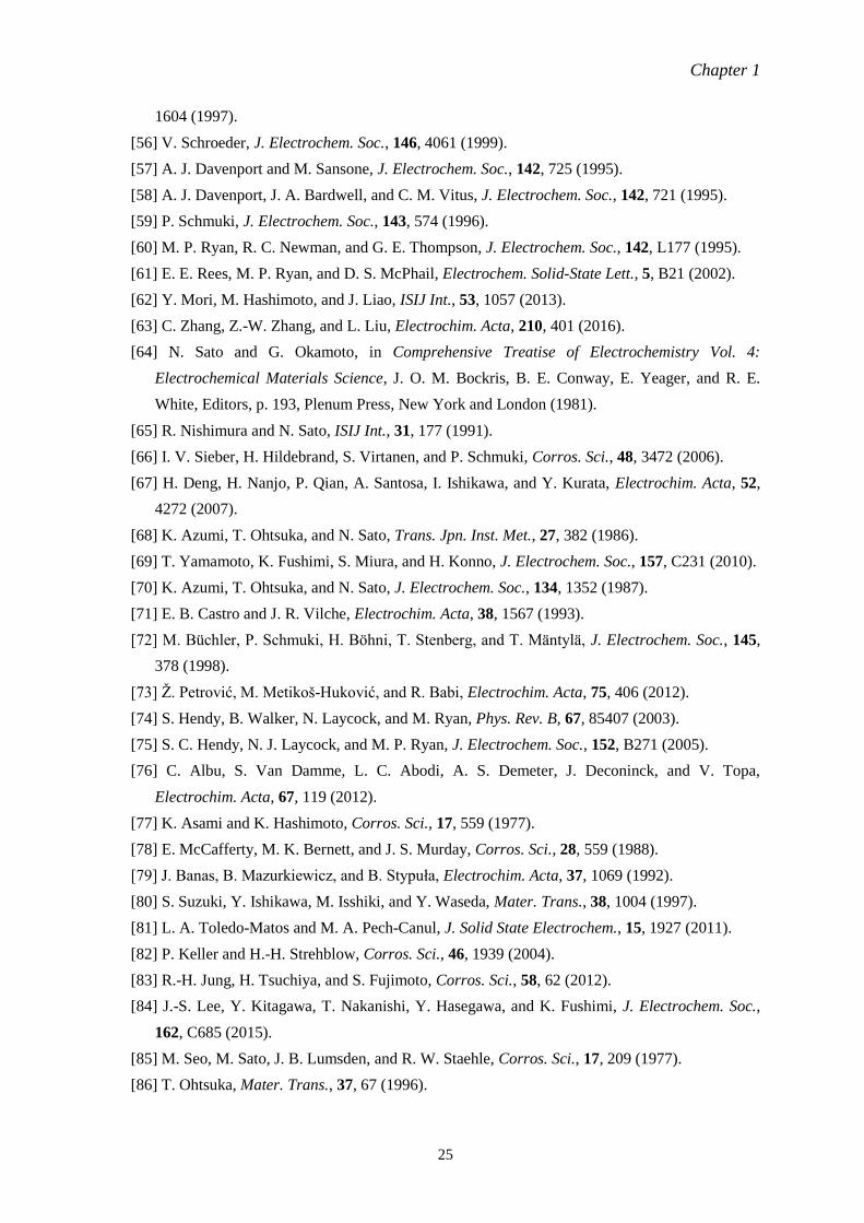
explosion of plant equipment. The Committee on Cost of Corrosion in Japan [2] reported that
corrosion costs in Japan at 1997, including economic losses and corrosion expenditures, to be 3.9
trillion JPY and 5.3 trillion JPY, as estimated by the Uhlig method and the Hoar method
respectively; these figures were equivalent to 0.77% and 1.02% to Japan’s gross national product
(GNP). Figure 1.1 shows the breakdown of corrosion costs as estimated by the Uhlig method.
Total costs, including direct and indirect costs, were estimated at 9.7 trillion JPY in 1997 (1.88%
of Japanese GNP) by the Input/Output analysis. From the viewpoint of reducing economic losses
and saving energy and resources, it is necessary to use metallic materials as long as possible, from
several decades to even hundreds of years. Longer service time in metallic materials is realized by
prevention strategies that minimize the progression of corrosion. A knowledge of corrosion
science and theories is necessary to develop appropriate strategies and aid in achieving a
sustainable society. Traditionally, the progress of corrosion has been estimated from the
macroscopic perspective by using the theories of uniform corrosion. In practice, non-uniform
Chapter 1
2
corrosion occurs on the surface of practical metallic materials, depending on the heterogeneous
characteristics of the surface (e.g., surface inclusions, metallographic texture, and crystallographic
orientation). Such heterogeneous corrosion leads to undesired breakdown in materials initiated by
localized corrosion that is difficult to predict with traditional theories of uniform corrosion. In
order to predict the progress of localized corrosion that occurs on practical materials, it is
necessary to elucidate the precise mechanisms of heterogeneous corrosion reactions from a
microscopic view.
1.1.2. Anisotropic corrosion
Metals and alloys demonstrate anisotropy for their characteristics because they have a
well-ordered crystal structure at the atomic level unless they are amorphous. Anisotropy affects
the properties of metallic materials and is used in several applications. For example, electrical
steel [3], which is a magnetic material used as the iron core of motors and electric transformers,
takes advantage of magnetic anisotropy. The iron core requires high magnetic flux density (i.e.,
high permeability) to maintain its magnetic energy. Since the magnetization easy axis of
body-centered cubic (bcc) iron is in the <0 0 1> direction, the orientation of crystal grains of the
electrical steel is controlled to face the <0 0 1> direction to the substrate normal direction (ND) by
rolling and annealing processes (Fig. 1.2), so that the steel achieves high magnetic flux density.
The activity of chemical reaction that occurs on the surface of metals and alloys is also
affected by anisotropy. The surface crystallographic orientation of metals and alloys affects their
corrosion reaction. Orientation-dependent corrosion behavior is reported using single crystals of
iron [4–6], copper [7], niobium [8], titanium [9], and zinc [10]. The oxide formation rates in both
air and aqueous solution depend on the surface crystallographic orientation.
Most metallic materials used in a wide range of industrial fields are polycrystalline, unless
there are specific reasons to use their monocrystalline forms, as with silicon chips for electronic
devices [11] and Ni-based alloys for gas turbine blades [12]. Since a polycrystalline material is
composed of numerous crystal grains, the surface of the material exposes many crystal planes,
each of which is characterized by individual crystallographic orientations, which means that the
surface activity of the polycrystalline material is not homogeneous. Grain-dependent corrosion of
polycrystalline metals has been reported for aluminum [13], copper [14–16], iron [17–20],
magnesium [21,22], titanium [23–27], zinc [28], and zirconium and tantalum [29].
Grain-dependent electrochemical activity for the redox reaction of Fe(II)/Fe(III) couples has also
been reported for polycrystalline platinum electrodes [30]. Through these studies, the broad trends
of grain-dependent corrosion on polycrystalline metals have been revealed; orientation-dependent
parameters such as surface energy and surface atomic density affect the dissolution and oxide
formation rates of substrate metals. However, the precise corrosion mechanism that depends on
the crystallographic orientation of the polycrystalline surface remains unclear. The progress of
anisotropic corrosion may initiate localized corrosion on polycrystalline materials. When the
Chapter 1
3
degradation rate of an oxide film and/or the dissolution rate of a substrate metal differ depending
on the surface orientation of the substrate, corrosion progresses preferentially at a local site where
corrosion resistivity is the lowest. The local site becomes a local anode, with the anodic
dissolution of the metal at that site accelerating due to the high anodic current density caused by
an extremely high ratio of local cathode/anode areas. This is the initiation of pitting corrosion,
which is a type of localized corrosion. In order to predict the initiation of localized corrosion, it is
necessary to elucidate the mechanism of grain-dependent corrosion that progresses on
polycrystalline materials.
1.2. Iron
Iron is the most commonly used metal in the world; it is employed in many industries as a
base element of steels. Figure 1.3 shows the total production of crude steel in the world from 1967
to 2015 [31]. Although Japanese steel production has not varied a great deal since the 1970s,
production in other countries has increased slightly, with China’s increasing dramatically since the
early decade of the 21st century. The drop in production in 2009 was due to the 2008 financial
crisis. According to a report by the Research Institute of Innovative Technology for the Earth
(RITE) in Japan [32], steel production will continue to increase in the coming decades due to
growing demand in developing countries. Thus, studying the corrosion behavior of iron will
become ever more important in supporting steel-based societies of the future.
High-purity iron is not used as a structural material since it is easily oxidized to rust by
oxygen in humid air and shows low toughness against external stress. However, knowing the
electrochemical behavior of pure iron is of great importance to understanding the essentials of
corrosion reactions on iron-based materials and steels.
1.2.1. General characteristics
Iron is in the transition metal family of elements (atomic number: 26, atomic weight: 55.85).
Its Clarke number, which indicates the ratio of elements that exist on the earth by weight percent
concentration, is 4.70 [33]. This is the second largest number among metal elements, trailing only
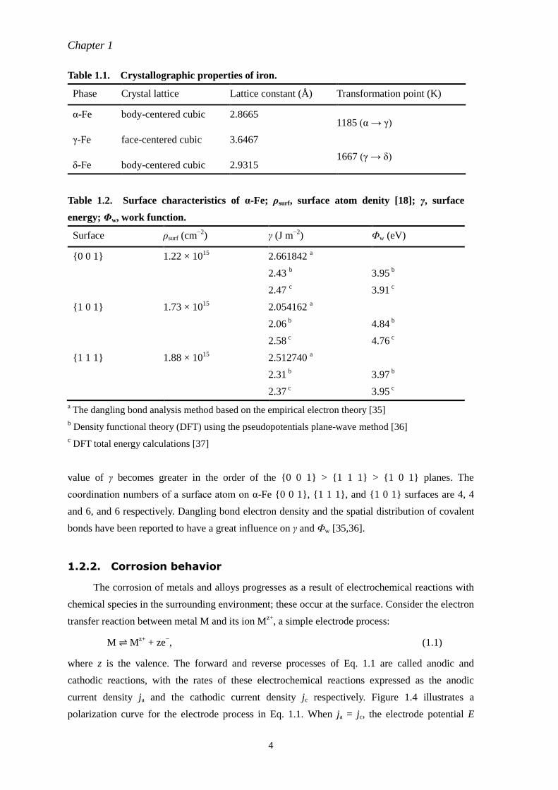
aluminum. The crystallographic properties of iron [34] are summarized in Table 1.1. Alpha-Fe
shows ferromagnetism at low temperature and paramagnetism at temperatures above the Curie or
A2 transformation point at 1044 K, with melting and boiling points of 1811 and 3003 K
respectively. When α-Fe showed paramagnetic properties, it was once called β-Fe. The electronic
properties of iron surfaces with low Miller indices have been studied with quantum chemistry
calculations. The calculated surface atom density ρsurf, the reported values of surface energy γ, and
the work function Φw, as calculated for the α-Fe {0 0 1}, {1 0 1}, and {1 1 1} planes, are
presented in Table 1.2. Although the authors report that γ shows some scattering, the average
Chapter 1
4
Table 1.1. Crystallographic properties of iron.
Phase Crystal lattice Lattice constant (Å) Transformation point (K)
α-Fe body-centered cubic 2.8665 1185 (α → γ)
γ-Fe face-centered cubic 3.6467
1667 (γ → δ) δ-Fe body-centered cubic 2.9315
Table 1.2. Surface characteristics of α-Fe; ρsurf, surface atom denity [18]; γ, surface
energy; Φw, work function.
Surface ρsurf (cm−2
) γ (J m−2
) Φw (eV)
{0 0 1} 1.22 × 10¹⁵
2.661842 a
2.43 b 3.95
b
2.47 c 3.91
c
{1 0 1} 1.73 × 10¹⁵
2.054162 a
2.06 b 4.84
b
2.58 c 4.76
c
{1 1 1} 1.88 × 10¹⁵
2.512740 a
2.31 b 3.97
b
2.37 c 3.95
c
a The dangling bond analysis method based on the empirical electron theory [35]
b Density functional theory (DFT) using the pseudopotentials plane-wave method [36]
c DFT total energy calculations [37]
value of γ becomes greater in the order of the {0 0 1} > {1 1 1} > {1 0 1} planes. The
coordination numbers of a surface atom on α-Fe {0 0 1}, {1 1 1}, and {1 0 1} surfaces are 4, 4
and 6, and 6 respectively. Dangling bond electron density and the spatial distribution of covalent
bonds have been reported to have a great influence on γ and Φw [35,36].
1.2.2. Corrosion behavior
The corrosion of metals and alloys progresses as a result of electrochemical reactions with
chemical species in the surrounding environment; these occur at the surface. Consider the electron
transfer reaction between metal M and its ion Mz+
, a simple electrode process:
M ⇌ Mz+ + ze
−, (1.1)
where z is the valence. The forward and reverse processes of Eq. 1.1 are called anodic and
cathodic reactions, with the rates of these electrochemical reactions expressed as the anodic
current density ja and the cathodic current density jc respectively. Figure 1.4 illustrates a
polarization curve for the electrode process in Eq. 1.1. When ja = jc, the electrode potential E
Chapter 1
5
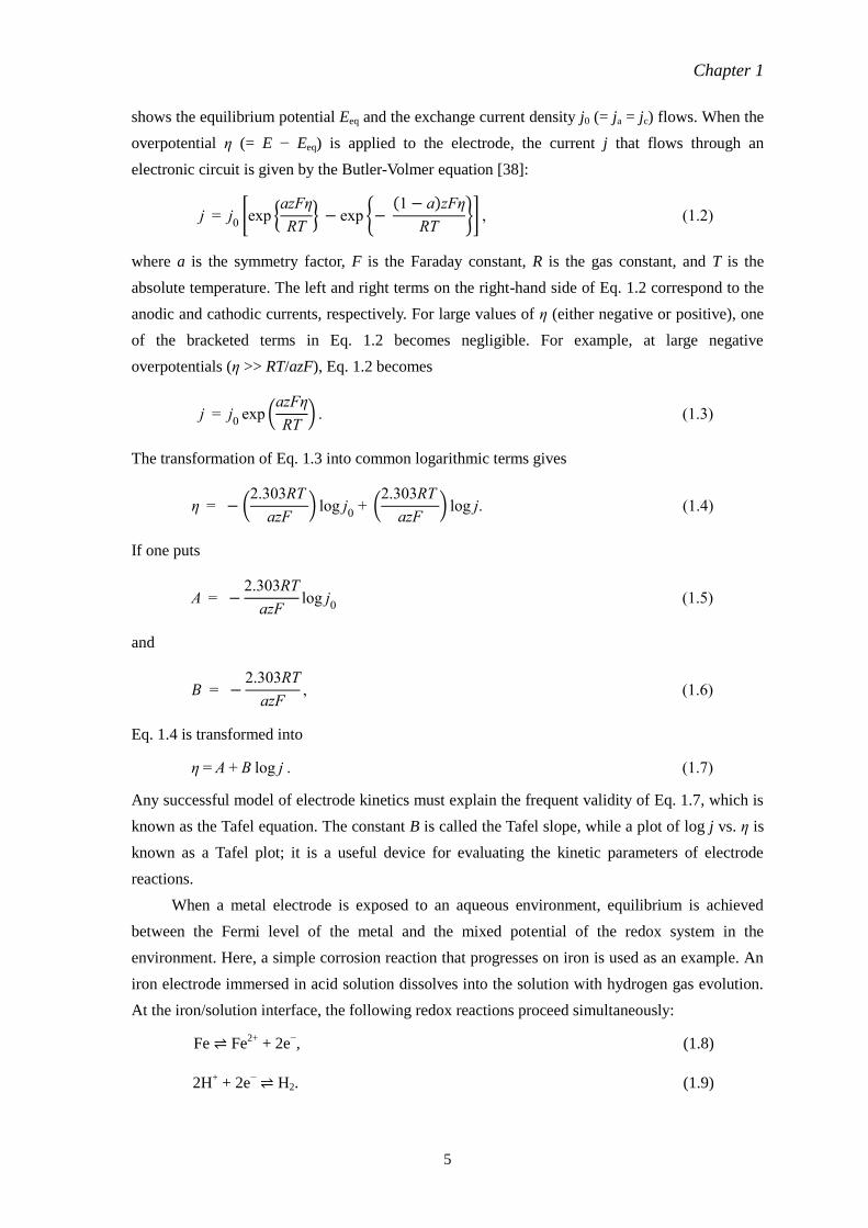
shows the equilibrium potential Eeq and the exchange current density j0 (= ja = jc) flows. When the
overpotential η (= E − Eeq) is applied to the electrode, the current j that flows through an
electronic circuit is given by the Butler-Volmer equation [38]:
j = j0
[exp {azFη
RT} − exp {−
(1 − a)zFη
RT}] , (1.2)
where a is the symmetry factor, F is the Faraday constant, R is the gas constant, and T is the
absolute temperature. The left and right terms on the right-hand side of Eq. 1.2 correspond to the
anodic and cathodic currents, respectively. For large values of η (either negative or positive), one
of the bracketed terms in Eq. 1.2 becomes negligible. For example, at large negative
overpotentials (η >> RT/azF), Eq. 1.2 becomes
j = j0
exp (azFη
RT) . (1.3)
The transformation of Eq. 1.3 into common logarithmic terms gives
η = − (2.303RT
azF) log j
0 + (
2.303RT
azF) log j. (1.4)
If one puts
A = −2.303RT
azFlog j
0 (1.5)
and
𝐵 = −2.303RT
azF, (1.6)
Eq. 1.4 is transformed into
η = A + B log j . (1.7)
Any successful model of electrode kinetics must explain the frequent validity of Eq. 1.7, which is
known as the Tafel equation. The constant B is called the Tafel slope, while a plot of log j vs. η is
known as a Tafel plot; it is a useful device for evaluating the kinetic parameters of electrode
reactions.
When a metal electrode is exposed to an aqueous environment, equilibrium is achieved
between the Fermi level of the metal and the mixed potential of the redox system in the
environment. Here, a simple corrosion reaction that progresses on iron is used as an example. An
iron electrode immersed in acid solution dissolves into the solution with hydrogen gas evolution.
At the iron/solution interface, the following redox reactions proceed simultaneously:
Fe ⇌ Fe2+
+ 2e−, (1.8)
2H+ + 2e
− ⇌ H2. (1.9)
Chapter 1
6
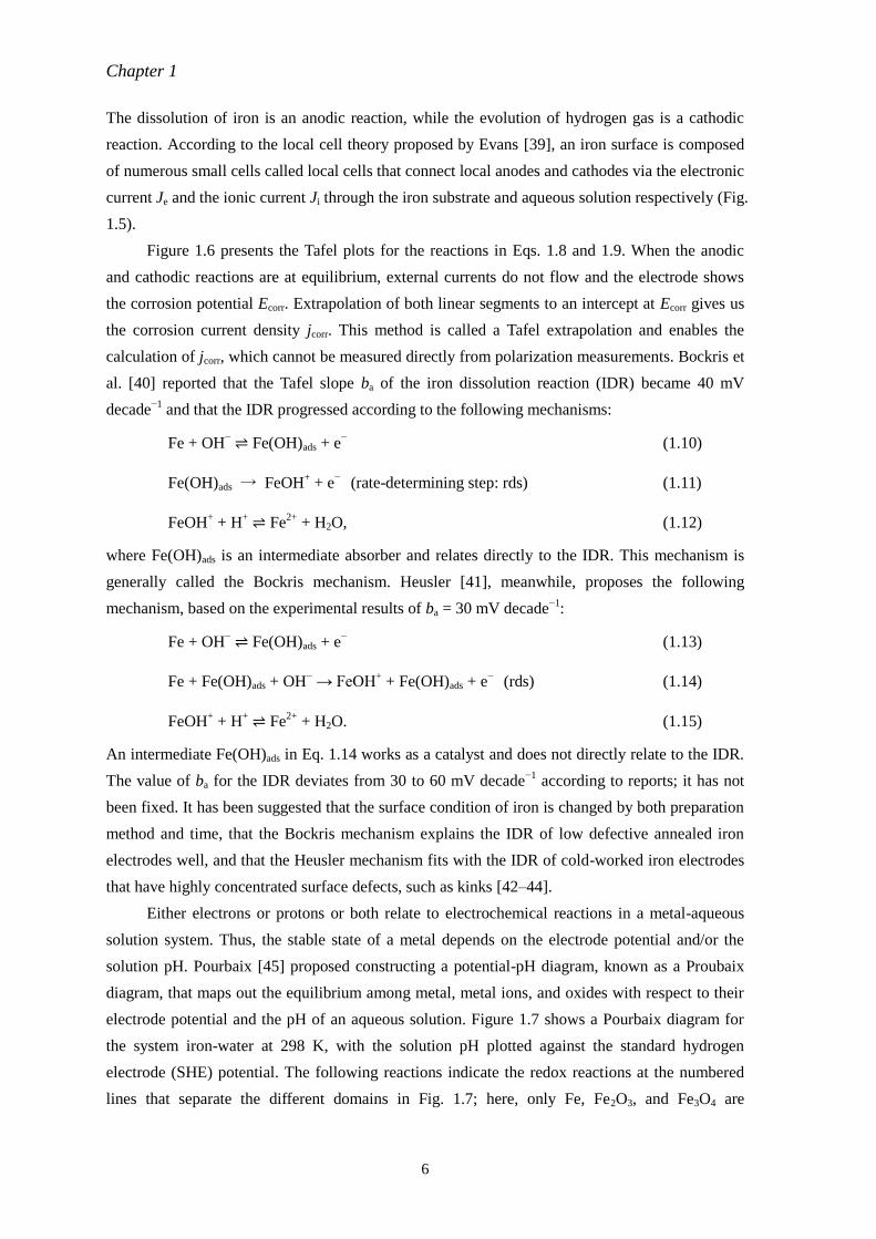
The dissolution of iron is an anodic reaction, while the evolution of hydrogen gas is a cathodic
reaction. According to the local cell theory proposed by Evans [39], an iron surface is composed
of numerous small cells called local cells that connect local anodes and cathodes via the electronic
current Je and the ionic current Ji through the iron substrate and aqueous solution respectively (Fig.
1.5).
Figure 1.6 presents the Tafel plots for the reactions in Eqs. 1.8 and 1.9. When the anodic
and cathodic reactions are at equilibrium, external currents do not flow and the electrode shows
the corrosion potential Ecorr. Extrapolation of both linear segments to an intercept at Ecorr gives us
the corrosion current density jcorr. This method is called a Tafel extrapolation and enables the
calculation of jcorr, which cannot be measured directly from polarization measurements. Bockris et
al. [40] reported that the Tafel slope ba of the iron dissolution reaction (IDR) became 40 mV
decade−1
and that the IDR progressed according to the following mechanisms:
Fe + OH− ⇌ Fe(OH)ads + e
− (1.10)
Fe(OH)ads → FeOH+ + e
− (rate-determining step: rds) (1.11)
FeOH+ + H
+ ⇌ Fe
2+ + H2O, (1.12)
where Fe(OH)ads is an intermediate absorber and relates directly to the IDR. This mechanism is
generally called the Bockris mechanism. Heusler [41], meanwhile, proposes the following
mechanism, based on the experimental results of ba = 30 mV decade−1
:
Fe + OH− ⇌ Fe(OH)ads + e
− (1.13)
Fe + Fe(OH)ads + OH− → FeOH
+ + Fe(OH)ads + e
− (rds) (1.14)
FeOH+ + H
+ ⇌ Fe
2+ + H2O. (1.15)
An intermediate Fe(OH)ads in Eq. 1.14 works as a catalyst and does not directly relate to the IDR.
The value of ba for the IDR deviates from 30 to 60 mV decade−1
according to reports; it has not
been fixed. It has been suggested that the surface condition of iron is changed by both preparation
method and time, that the Bockris mechanism explains the IDR of low defective annealed iron
electrodes well, and that the Heusler mechanism fits with the IDR of cold-worked iron electrodes
that have highly concentrated surface defects, such as kinks [42–44].
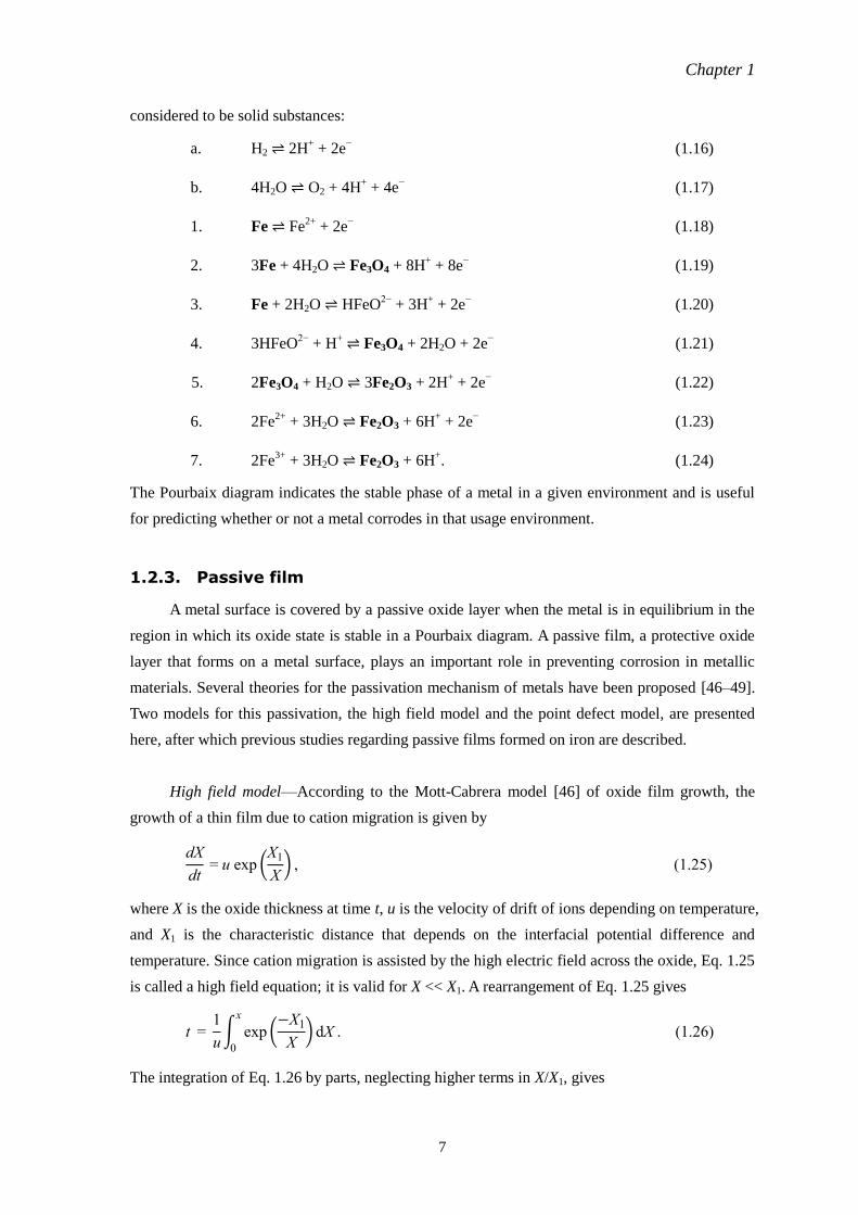
Either electrons or protons or both relate to electrochemical reactions in a metal-aqueous
solution system. Thus, the stable state of a metal depends on the electrode potential and/or the
solution pH. Pourbaix [45] proposed constructing a potential-pH diagram, known as a Proubaix
diagram, that maps out the equilibrium among metal, metal ions, and oxides with respect to their
electrode potential and the pH of an aqueous solution. Figure 1.7 shows a Pourbaix diagram for
the system iron-water at 298 K, with the solution pH plotted against the standard hydrogen
electrode (SHE) potential. The following reactions indicate the redox reactions at the numbered
lines that separate the different domains in Fig. 1.7; here, only Fe, Fe2O3, and Fe3O4 are
Chapter 1
7
considered to be solid substances:
a. H2 ⇌ 2H+ + 2e
− (1.16)
b. 4H2O ⇌ O2 + 4H+ + 4e
− (1.17)
1. Fe ⇌ Fe2+
+ 2e− (1.18)
2. 3Fe + 4H2O ⇌ Fe3O4 + 8H+ + 8e
− (1.19)
3. Fe + 2H2O ⇌ HFeO2−
+ 3H+ + 2e
− (1.20)
4. 3HFeO2−
+ H+ ⇌ Fe3O4 + 2H2O + 2e
− (1.21)
5. 2Fe3O4 + H2O ⇌ 3Fe2O3 + 2H+ + 2e
− (1.22)
6. 2Fe2+
+ 3H2O ⇌ Fe2O3 + 6H+ + 2e
− (1.23)
7. 2Fe3+
+ 3H2O ⇌ Fe2O3 + 6H+. (1.24)
The Pourbaix diagram indicates the stable phase of a metal in a given environment and is useful
for predicting whether or not a metal corrodes in that usage environment.
1.2.3. Passive film
A metal surface is covered by a passive oxide layer when the metal is in equilibrium in the
region in which its oxide state is stable in a Pourbaix diagram. A passive film, a protective oxide
layer that forms on a metal surface, plays an important role in preventing corrosion in metallic
materials. Several theories for the passivation mechanism of metals have been proposed [46–49].
Two models for this passivation, the high field model and the point defect model, are presented
here, after which previous studies regarding passive films formed on iron are described.
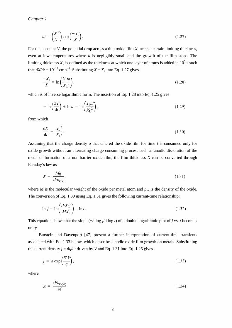
High field model—According to the Mott-Cabrera model [46] of oxide film growth, the
growth of a thin film due to cation migration is given by
dX
dt = u exp (
X1
X) , (1.25)
where X is the oxide thickness at time t, u is the velocity of drift of ions depending on temperature,
and X1 is the characteristic distance that depends on the interfacial potential difference and
temperature. Since cation migration is assisted by the high electric field across the oxide, Eq. 1.25
is called a high field equation; it is valid for X << X1. A rearrangement of Eq. 1.25 gives
t = 1
u∫ exp (
−X1
X) dX . (1.26)
x
0
The integration of Eq. 1.26 by parts, neglecting higher terms in X/X1, gives
Chapter 1
8
ut = (X 2
X1
) exp (−X1
X) . (1.27)
For the constant V, the potential drop across a thin oxide film X meets a certain limiting thickness,
even at low temperatures where u is negligibly small and the growth of the film stops. The
limiting thickness XL is defined as the thickness at which one layer of atoms is added in 105 s such
that dX/dt = 10−13
cm s−1
. Substituting X = XL into Eq. 1.27 gives
−X1
X = ln (
X1ut
XL2
) , (1.28)
which is of inverse logarithmic form. The insertion of Eq. 1.28 into Eq. 1.25 gives
− ln (dX
dt) + ln u = ln (
X1ut
XL2
) , (1.29)
from which
dX
dt =
XL2
X1t. (1.30)
Assuming that the charge density q that entered the oxide film for time t is consumed only for
oxide growth without an alternating charge-consuming process such as anodic dissolution of the
metal or formation of a non-barrier oxide film, the film thickness X can be converted through
Faraday’s law as
X = Mq
zFρOX
, (1.31)
where M is the molecular weight of the oxide per metal atom and ρox is the density of the oxide.
The conversion of Eq. 1.30 using Eq. 1.31 gives the following current-time relationship:
ln j = ln (zFXL
2
MX1
) − ln t . (1.32)
This equation shows that the slope (−d log j/d log t) of a double logarithmic plot of j vs. t becomes
unity.
Burstein and Davenport [47] present a further interpretation of current-time transients
associated with Eq. 1.33 below, which describes anodic oxide film growth on metals. Substituting
the current density j = dq/dt driven by V and Eq. 1.31 into Eq. 1.25 gives
j = A exp (B’V
q) , (1.33)
where
A = zFuρ
OX
M (1.34)
Chapter 1
9
and
B’V = zFρ
OX X1
M. (1.35)
Substituting Eqs. 1.31, 1.33, and 1.34 into the logarithmic form of Eq. 1.27 gives
B’V
q = − ln (
B’V At
q2) , (1.36)
from which insertion into the logarithmic form of Eq. 1.33 gives
ln (j
A) = − ln [
At {ln ( j/A)}2
B’V] . (1.37)
After rearrangement, Eq. 1.37 becomes
j = B’V
t {ln (j/A)}2. (1.38)
Equation 1.38 provides an expression that describes high field growth kinetics in terms of current
and time. Rearranging Eq. 1.38 and taking common logarithms gives
log j = log A + (B’V)
1/2
2.303 ( jt)−1/2
. (1.39)
Thus, a plot of log j vs. (jt)−1/2
shows a straight line with gradient (B’V)1/2
/2.303 and intercept
log A. The current decays according to direct logarithmic kinetics in Eq. 1.32, in which (−d log j/d
log t) = 1 requires the product of j and t to be a constant. Thus, the current-time relation observed
with direct logarithmic kinetics appears as a vertical line parallel to the log j axis on a plot of log j
vs. (jt)−1/2
. This model, when considered with the ohmic potential drop between the working
electrode and the reference electrode, shows good agreement with current-time transients
describing passivating oxide film growth on iron and titanium alloys.
Point defect model—The point defect model was first proposed by Chao, Lin, and
Macdonald [48] to account for the growth kinetics of a passive film on a metal surface; it has been
refined considerably by Macdonald [49]. The model is based on the following assumptions: (i)
whenever the external potential Eext is nobler than the Flade potential, where a metal electrode
transits from the passive state to the active state, a continuous passive film will form on the
surface of the metal; (ii) the passive film has a high concentration of defects: point defect species
(VMx’ the metal vacancy, VO•• the oxygen vacancy, e’ the electrons, and h
• the holes) are expected
in the passive film, and the Kröger-Vink notation is adopted to designate the point defect species;
(iii) the field strength is a function of the film’s chemical and electrical characteristics and is thus
independent of film thickness, even for potentiostatic conditions; (iv) the electrons e’ and holes h•
in the film matrix are in their equilibrium states, and the electrochemical reactions involving e’ (or
h•) are rate-controlled at either the metal/film (m/f) or the film/solution (f/s) interface, while the
Chapter 1
10
rate-controlling step for those processes that involve VMx’ and VO•• (i.e., film growth) is assumed
to be the transport of the vacancies across the film.
Figure 1.8 shows the potential-position relationship between working and reference
electrodes, with the following relation obtained:
Eext + ∆ϕR
= ∆ϕm/f
+ ∆ϕf + ∆ϕ
f/s, (1.40)
where ∆ϕm/f, ∆ϕf/s, and ∆ϕR are potential drops at the m/f, f/s, and solution/reference electrode
interfaces and ∆ϕf is the potential drop across the film. The following two reactions occur at the
m/f interface:
m ⇄ MM + x
2VO•• + xe’ (1.41)
m + VMx’ ⇄ MM + xe’, (1.42)
where m represents the metal atom in the metal and MM is the metal cation in the film. When the
m/f interface is at equilibrium
μm
= μMM
+ x
2μ
VO•• + xFϕ
f’ + x𝜇e’ − xFϕ
m, (1.43)
where ϕf’ and ϕm are the flat band potentials for the film and metal at the m/f interface,
respectively, and μι is the chemical potential of species ι. The standard Gibbs energy ∆G41º of the
reaction of Eq. 1.41 is defined as
ΔG41º = μMM
º + x
2μ
VO•• º + xμ
e’º − μ
mº (1.44)
by selecting appropriate the standard states
μm
= μm
º , (1.45a)
μMM
= μMM
º , (1.45b)
𝜇e’ = μe’
º , (1.45c)
ϕm
− ∆ϕf
= ∆ϕm/f
, (1.45d)
and
μVO
•• = μVO
•• º + RT ln aVO••(m/f) , (1.46)
where aVO••(m/f) is the activity of VO
•• at the m/f interface. Substituting Eqs. 1.44–46 into Eq. 1.43
yields
aVO••(m/f) = exp {
2FΔϕm/f
− (2/x)ΔG41º
RT} . (1.47)
A similar treatment of Eq. 1.42 gives
Chapter 1
11
aVMx’(m/f) = exp (ΔG42º − 𝑥FΔϕ
m/f
RT) , (1.48)
where ∆G42º is the standard Gibbs energy of the reaction in Eq. 1.42. Assuming that the
interaction between point defects is negligible—i.e., the point defects behave as an ideal
solution—the activity coefficient is unity and the concentrations CVO••(m/f) and CVMx’(m/f) of VO
••
and VMx’ at the m/f interface are estimated as
CVO••(m/f) =
NA
Ω exp {
2FΔϕm/f
− (2/x)ΔG41º
RT} (1.49)
and
CVMx’(m/f) =NA
Ω exp (
ΔG42º − 𝑥FΔϕm/f
RT) , (1.50)
where NA is the Avogadro number and Ω is the molecular volume of oxide.
At the f/s interface, two other reactions occur:
VO•• + H2O ⇄ 2H
+(aq) + OO (1.51)
and
MM ⇄ VMx’ + Mx+
(aq), (1.52)
where Mx+
(aq) is the hydrated metal cation in electrolyte solution. The concentration CVO••(f/s) of
VO•• at the f/s interface is obtained in the same manner as the calculation of Eq. 1.49 with ∆G51º,
the standard Gibbs energy of the reaction of Eq. 1.51:
CVO••(f/s) =
NA
Ω exp [(
ΔG51º − xFΔϕm/f
RT) − 4.606 pH] . (1.53)
From the Schottky pair reaction,
Null ⇄ VMx’ + x
2VO•• . (1.54)
Therefore,
CVMx’∙ [CVO
•• ]x/2
= [ NA
Ω ]
1 + (x 2⁄ )
exp (− ΔGSº
RT) , (1.55)
where ∆GSº is the Gibbs standard energy change for the Schottky pair reaction and the multiplier
on the right-hand side arises due to the use of concentrations rather than activities. From Eqs. 1.53
and 1.54, CVO••(f/s) is obtained as
CVO••(f/s) =
NA
Ω exp {
xFΔϕm/f
− ΔGSº − (x 2⁄ )ΔG51º
RT + 2.303 x pH} . (1.56)
Chapter 1
12
Since it is clear from Eqs. 1.41, 1.42, 1.51, and 1.52 that the diffusion of VO•• (or equivalently,
oxygen anion) results in film growth, the diffusion rate of VO•• is equivalent to film growth
kinetics. Thus,
dX
dt =
Ω
NA
JVO•• , (1.57)
where Ω is the molar volume per cation and JVO•• is the flux of VO
•• per unit area per unit time.
From the generalized Fick’s first law, JVO•• can be calculated as
JVO•• = 2KD*
VO••
CVO••(m/f) exp(2KX) − CVO
••(f/s)
exp(2KX) − 1 , (1.58)
where D*VO
•• is the electrochemical diffusivity of VO••
and K is equal to FεF/RT (εF is the field
strength, εF = Δϕf/X). Assuming that Δϕ
f/s is a function of applied potential and solution pH but
is independent of film thickness, Δϕf/s
is described as
Δϕf/s
= αEext + β pH + ϕf/s
º , (1.59)
where α and β are coefficients and Δϕf/s
º is the value of Δϕf/s
when Eext = 0 and pH = 0. From
Eqs. 1.40 and 1.59, an expression for Δϕm/f
is derived as
Δϕm/f
= (1 − α)Eext
− β pH − Δϕf/s
º + ΔϕR
− εFX , (1.60)
where ΔϕR
is treated as a constant because the reference electrode is not polarized. Substituting
Eqs. 1.49, 1.56, 1.58, 1.59, and 1.60 into Eq. 1.57 gives
dX
dt =
A(B − 1)
exp(2KX) − 1, (1.61)
where
A = 2KD*VO
•• exp {−2F
RT (αEext + β pH + Δϕ
f/sº) +
ΔG51º
RT− 4.606 pH} (1.62)
and
B = exp {2F
RT (Eext + Δϕ
R) −
2ΔG41º
xRT −
ΔG51º
RT + 4.606 pH} . (1.63)
Under potentiostatic polarization, Eext is equal to the applied potential Eapp and independent of the
film thickness X. Eq. 1.61 can be integrated directly, since
∫ [exp(2KX) − 1] d(2KX) = ∫ 2KA(B − 1)dt , (1.64)t
0
X
0
which therefore yields
exp(2KX) − 2KX − 1 = 2KA (B − 1) t. (1.65)
Equation 1.65 is the integrated rate law for film growth.
The field strength εF for most anodic films is of the order of 106 V cm
−1 at room
Chapter 1
13
temperature. Thus, 2KX = 2FεF/RT ~ 0.76 X. This means that whenever X ≥ 0.5 nm, exp(2KX) >>
2KX >> 1 and Eq. 1.65 can be simplified to
exp(2KX) = 2KA (B − 1) t (1.66)
or
X = 1
2K[ln {2KA(B − 1)} + ln t]. (1.67)
Equation 1.67 has the form of the logarithmic growth raw. Furthermore, when the current j is
consumed only for oxide growth, it is written as
j = 2F NA
Ω
dX
dt. (1.68)
Substituting Eq. 1.68 into Eq. 1.67 gives
j = FNA
KΩt−1. (1.69)
Equation 1.69 indicates that a current transient varies inversely with time.
On the other hand, for very small values of X, Eq. 1.65 can be reduced to
X = {A(B − 1)
Kt}
1/2
. (1.70)
This gives a relation of
j ∝ dX
dt =
1
2{
A(B − 1)
K}
1 2⁄
t −1 2⁄ . (1.71)
Equation 1.71 indicates that a current transient varies with the square root of time.
Due to their importance in industry, the passivation mechanism and kinetics of iron have
been intensively investigated for more than half a century. In many cases, the passivation behavior
and the property of the passive film on iron were studied in neutral aqueous solution, where the
dissolution of the film and the substrate iron through the film into electrolyte solution was
negligible and the change in the film property during measurements was minimal.
The structure of a passive film formed on iron in neutral borate buffer solution has been
studied using several investigative techniques. An electron diffraction study [50] demonstrated
that the film had a bi-layered spinel structure of inner Fe3O4 and outer γ-Fe2O3. A further electron
diffraction study [51] showed that it was not possible to make a definitive distinction between
Fe3O4 and γ-Fe2O3, but the film had a fine-grained crystalline spinel structure consisting of a
varying iron concentration from the metal/oxide interface to the oxide/solution interface. On the
other hand, cathodic reduction combined with ellipsometry and chemical analysis [52] led to
another film structure with a barrier Fe(III) oxide layer in contact with the metal and a deposit
Chapter 1
14
hydrated Fe(III) oxide or oxyhydroxide layer on the barrier layer. A bi-layer film with inner
anhydrous and outer hydrated layers was also found by electron spectroscopy for chemical
analysis (ESCA) and secondary ion mass spectroscopy (SIMS) [53]. Nowadays, ESCA is known
as X-ray photoelectron spectroscopy (XPS). By contrast, the results of surface-enhanced Raman
spectroscopy (SERS) indicated that the passive film was hydrated spinel-based oxide [54,55] or a
bi-layer of inner Fe3O4 or defected γ-Fe2O3 and outer unknown ferric oxide or hydroxide [56].
More recently, high resolution in situ X-ray absorption near edge structure (XANES)
demonstrated that the obtained absorption edge peak was consistent with the proposed
Fe3O4/γ-Fe2O3 structure or a disordered structure with distorted coordination polyhedral [57–59].
A study using in situ synchrotron X-ray diffraction (XRD) [6] suggested that the passive film was
neither Fe3O4 nor γ-Fe2O3, but was instead a new phase—the LAMM phase—that had a spinel
structure with a different defect structure. The crystalline nature of the passive film was confirmed
by in situ scanning tunneling microscopy (STM) [60]. Later STM work [61] suggested the
presence of nanoscale oxide grains in the LAMM phase, but did not reveal the complete structure
of the film. As noted above, while several structures of passive films on iron have been proposed,
there are presently no definitive studies of the nature of the passive films, with most recent studies
suggesting a structure related to Fe3O4 and γ-Fe2O3.
Due to the ultra-thin nature—in the range of a few nanometers—of passive films, direct
observation of the film structure has rarely been demonstrated. Recently, a focused ion beam
(FIB) technique made the preparation of a thin sample film for observation with transmission
electron microscopy (TEM) easier than previously possible. A cross section of a few nanometer
thick passive film on 316L stainless steel was observed by means of FIB-TEM [62,63]. However,
the question remained whether or not that ex situ observation in vacuum examined the film
structure as it exists in situ, so in situ ellipsometry under polarization measurements have been
intensively demonstrated to evaluate the thickness of the passive film on iron in neutral borate
buffer solution. The thickness of the passive film evaluated by ellipsometry ranged from ca. 2–7
nm depending on the formation potential, electrolyte pH, and anion species and concentration in
electrolyte solution [64–67].
The electric property of the passive film has been evaluated by means of electrochemical
impedance spectroscopy (EIS). The charge transfer resistance Rct for ionic and electronic
conductions through the film is usually obtained from curve fitting of impedance spectra obtained
from EIS measurements. Values of Rct = 0.2‒1.5 MΩ cm2 were reported for the passive film
formed on iron in borate solution [68,69]. Mott-Schottky (MS) analysis based on EIS evaluated an
n-type semiconductive property of the passive film from the positive slope in the so-called MS
plot, which draws the variation of inverse squares of space-charge capacitance as a function of
evaluation potential. The passive film showed a flat band potential Efb of 0.3‒0.5 V versus
reversible hydrogen electrode (RHE) potential and a donor density ND of 2‒30 × 1020
cm−3
[69–
73]. The slight scattering observed in these parameters is due to differences in formation potential
Chapter 1
15
and time. The value of Efb was almost constant at potentials less than 1.5 V (RHE) [70], at which
the oxygen evolution reaction occurred. On the contrary, ND decreased with increasing formation
potential or oxidation time due to the reduction of defect sites [70]. A study of MS analysis and
photocurrent measurements [72] concluded that the doping species of the passive film was Fe(II)
ion and the further oxidation of Fe(II) into Fe(III) in the film decreased ND in the high potential
region.
Recent developments in the field of computer science have enabled the use of
computational calculation for the investigation of the growth mechanism and electronic property
of the passive film. Density functional theory (DFT) calculations suggested that the proposed
LAMM phase was metastable with respect to the iron substrate [74] and that cation transport
during oxide growth was dominated by grain boundary diffusion [75]. A numerical simulation
based on a finite element method showed that Fe(III) interstitials and oxygen vacancies were the
species responsible for the transport of mass in the oxide film [76].
1.3. Analytical techniques
In this section, typical techniques used to analyze the structure, composition, and property
of oxide films formed on iron are introduced, along with practical examples.
1.3.1. Vacuum analysis
X-ray photoelectron spectroscopy is a highly sensitive surface analysis technique that
examines the composition, chemical state, and electronic state of the elements that exist on a
sample surface. Photoelectron spectra are obtained by simultaneously measuring the kinetic
energy Ek and the number of electrons that escape from the top ca. 10 nm of the sample by X-ray
irradiation. Generally, photoelectron intensity is shown as a function of the binding energy Eb
between an electron and an atomic nucleus, according to the following relation:
Eb = hν – Ek – Φw, (1.72)
where hν is the photon energy of an incident X-ray (h is the Plank constant and ν is the frequency)
and Φw is the work function dependent on both the spectrometer and the sample [77]. Figure 1.9
illustrates the emission of a photoelectron caused by the incident X-ray. Taking advantage of its
surface sensitivity, XPS has used to investigate the composition and structure of ultra-thin passive
films [78–80]. A passive film formed on pure iron in neutral solution was studied ex situ after
being transferred from electrolyte solution to the vacuum chamber of a spectrometer; a bi-layer
film structure with an inner iron oxide containing both Fe(II) and Fe(III) and outer hydrated
oxides was reported [81]. Angle-resolved XPS found that a passive film formed in phosphate
buffer solution contained a significant amount of phosphate in the outer part of the film, whereas
boron species were not significantly incorporated into the film formed in borate buffer solution
Chapter 1
16
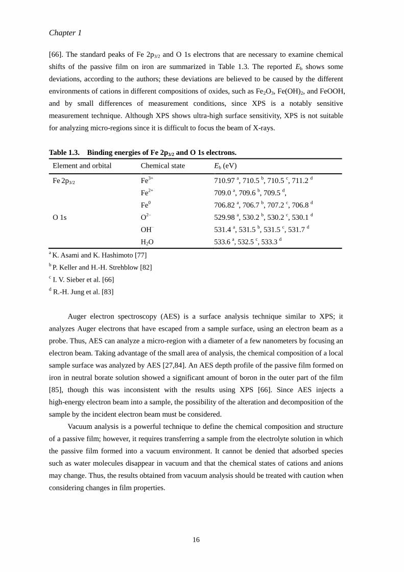
[66]. The standard peaks of Fe 2p3/2 and O 1s electrons that are necessary to examine chemical
shifts of the passive film on iron are summarized in Table 1.3. The reported Eb shows some
deviations, according to the authors; these deviations are believed to be caused by the different
environments of cations in different compositions of oxides, such as Fe2O3, Fe(OH)2, and FeOOH,
and by small differences of measurement conditions, since XPS is a notably sensitive
measurement technique. Although XPS shows ultra-high surface sensitivity, XPS is not suitable
for analyzing micro-regions since it is difficult to focus the beam of X-rays.
Table 1.3. Binding energies of Fe 2p3/2 and O 1s electrons.
Element and orbital Chemical state Eb (eV)
Fe 2p3/2 Fe3+
710.97 a, 710.5
b, 710.5
c, 711.2
d
Fe2+
709.0 a, 709.6
b, 709.5
d,
Fe0 706.82
a, 706.7
b, 707.2
c, 706.8
d
O 1s O2–
529.98 a, 530.2
b, 530.2
c, 530.1
d
OH– 531.4
a, 531.5
b, 531.5
c, 531.7
d
H2O 533.6 a, 532.5
c, 533.3
d
a K. Asami and K. Hashimoto [77]
b P. Keller and H.-H. Strehblow [82]
c I. V. Sieber et al. [66]
d R.-H. Jung et al. [83]
Auger electron spectroscopy (AES) is a surface analysis technique similar to XPS; it
analyzes Auger electrons that have escaped from a sample surface, using an electron beam as a
probe. Thus, AES can analyze a micro-region with a diameter of a few nanometers by focusing an
electron beam. Taking advantage of the small area of analysis, the chemical composition of a local
sample surface was analyzed by AES [27,84]. An AES depth profile of the passive film formed on
iron in neutral borate solution showed a significant amount of boron in the outer part of the film
[85], though this was inconsistent with the results using XPS [66]. Since AES injects a
high-energy electron beam into a sample, the possibility of the alteration and decomposition of the
sample by the incident electron beam must be considered.
Vacuum analysis is a powerful technique to define the chemical composition and structure
of a passive film; however, it requires transferring a sample from the electrolyte solution in which
the passive film formed into a vacuum environment. It cannot be denied that adsorbed species
such as water molecules disappear in vacuum and that the chemical states of cations and anions
may change. Thus, the results obtained from vacuum analysis should be treated with caution when
considering changes in film properties.
Chapter 1
17
1.3.2. Optical measurements
Using light as a probe, optical measurement techniques enable the analysis of a sample
surface without any destruction of chemical species and do not require a specific experimental
environment. Taking advantage of these characteristics, several optical measurement techniques
have been developed and applied to the analysis of oxide films formed on iron.
Raman spectroscopy investigates the vibrational structure of a substance, generally using
visible light as a probe (Fig. 1.10) to identify the composition of the substance by comparing it
with standards. The composition of a passive film on iron was studied by means of Raman
spectroscopy, with Raman peaks assigned to a hydrated form of Fe3O4 and γ-Fe2O3 or Fe3–δO4
[86]. However, observation of clear Raman peaks in the passive film and in situ observation were
difficult due to its ultrathin structure. This obstacle has been overcome by a SERS technique that
enhances Raman scattering of substances by nanostructures of a substrate surface, which enables
in situ measurements of Raman spectra. The passive film on iron was investigated by means of in
situ SERS by depositing nanoparticles of silver [54] and gold [56]. Recently, confocal Raman
spectroscopy that confines measurement area to ca. 1 µm in a diameter has been performed to
investigate a local sample surface; Raman mapping was also conducted [87].
Ellipsometry is an effective method for determining the thickness and optical constants of a
thin oxide layer on a flat substrate. The principle of ellipsometry is described in Chapter 2. Due to
its high thickness resolution of sub-nanometers, ellipsometry has been intensively used to
investigate the thicknesses and structures of anodic oxide films on metals [88–90]. A relatively
thin thermal oxide film formed on an interstitial free steel has also been reported [91]. Since
ellipsometry is a non-destructive technique, it is suitable for in situ measurements of the
formation and degradation of oxide films on metals and alloys. An ellipsometer combined with an
electrochemical cell observed in situ optical changes of an iron surface during potentiostatic
anodic polarization and galvanostatic cathodic reduction [92]. The structure of a passive film on
iron was precisely revealed by in situ ellipsometry [93]. In situ ellipso-microscopy observed local
film degradation of a passive film on titanium [27]. By using a laser as a probe light, the spot area
on a sample surface can be confined to several micrometers in diameter. Laser-probed
ellipsometry with high lateral resolution has enabled the visualization of the two-dimensional
(2D) distribution of ellipsometric parameters of the sample surface. For example, the thickness
distributions of organic thin films on a gold substrate [94] and a ZnO film on a silicon wafer [95]
were observed by 2D ellipsometry. This technique is a promising method for elucidating the
surface heterogeneity of oxidized polycrystalline metals. Thus, in situ 2D ellipsometry, which is a
combination of 2D ellipsometry and electrochemical measurements, is thought to be an effective
technique for investigating the surface heterogeneity of oxidized polycrystalline metals.
1.3.3. Micro-electrochemical measurement methods
For the purpose of investigating the local electrochemical behavior of polycrystalline
Chapter 1
18
metals and alloys, several micro-electrochemical measurement techniques have been developed
by researchers [96–99]. The two major techniques, scanning electrochemical microscopy (SECM)
and a micro-capillary cell (MCC) method, are outlined.
SECM is a kind of scanning probe microscopy developed by Bard et al. [96,97] as a tool for
imaging the electrochemical activity of a sample electrode surface. The probe tip of a
micro-electrode moves normally to the sample surface (in the z direction) to evaluate the diffusion
layer on the surface, or can be scanned at constant z across the surface (in the x-y directions) to
achieve an image map of electrochemical reactivity of the surface. This technique was applied to
evaluate the heterogeneity of an anodic passive film formed on polycrystalline metals [15,17,23].
When SECM is conducted in tip-generation/substrate-collection (TG/SC) mode (Fig. 1.11), the
oxidation and reduction of a redox couple mediator such as Fe(CN)64−
/Fe(CN)63−
occur
respectively at the tip and substrate kept at constant potential. The mediator is oxidized at the tip
and the oxidized mediator is reduced at a passive film formed on the substrate metal. The probe
current reflects the generation rate of reduced species on the film and thus depends on the electron
tunneling through the passive film. Since the tunneling current is affected by the electronic
property and thickness of the film, SECM can evaluate the heterogeneity of the electronic
property and/or thickness of a passive film formed on a whole polycrystalline metal surface.
The MCC (also called a capillary microcell or a micro-droplet cell) method was developed
independently by Böhni et al. [98] and Lohrengel et al. [99] in the late 1990s. It uses a narrow
capillary filled with electrolyte solution and places a small droplet on a sample surface. The
contact area of the droplet represents the working electrode in an electrochemical cell. The tip
diameter of the capillary varies from 20 µm to a few millimeters and defines the electrode
diameter of the MCC. Usually, insulating narrow tubes of glasses or polymers are used for the
capillary, while at times metallic tubes of platinum, gold, and stainless steel are used for the
capillary, which also works as a counter electrode. MCC has the following advantages comparing
with ordinary macro-electrochemical cells: (i) pretreatment of a sample with insulating coating,
resin-embedding, or the like is not necessary; (ii) an electrochemical measurement is conducted
only at a desired micro-region of a sample electrode; (iii) it consumes only a small amount of
electrolyte solution for a single measurement (on the order of micro-liters). The MCC technique is
divided into two groups, according to the structure of a capillary tip/sample electrode interface.
Figure 1.12a shows the cell structure of a meniscus type MCC [98]. A capillary tip maintains a
constant distance from a substrate and makes a droplet as a micro-electrode between the tip and
the substrate surface. Since the capillary tip does not contact the substrate directly, it is possible to
scan the micro-electrode laterally during electrochemical measurements. However, it is difficult to
keep the electrode area constant, because the shape of the droplet is governed by the surface
tension and wettability of the electrolyte solution. Figure 1.12b shows a gasket type MCC [99]. A
silicone rubber is placed on the tip and the capillary directly contacts the substrate surface. A
micro-electrode is formed in the confined area made up of the capillary, gasket, and sample
Chapter 1
19
substrate. Although it is difficult to scan gasket type MCCs, they realize a constant electrode area
at each measurement.
1.4. Previous study on orientation-dependent
corrosion of iron
The corrosion behavior of iron has been studied heavily, as outlined above; it has been
reported that surface crystallographic orientation affected corrosion behavior [4–6]. However, the
progress of orientation-dependent corrosion of iron is difficult to explain using previous corrosion
theories and has been frequently overlooked when researchers have examined the corrosion
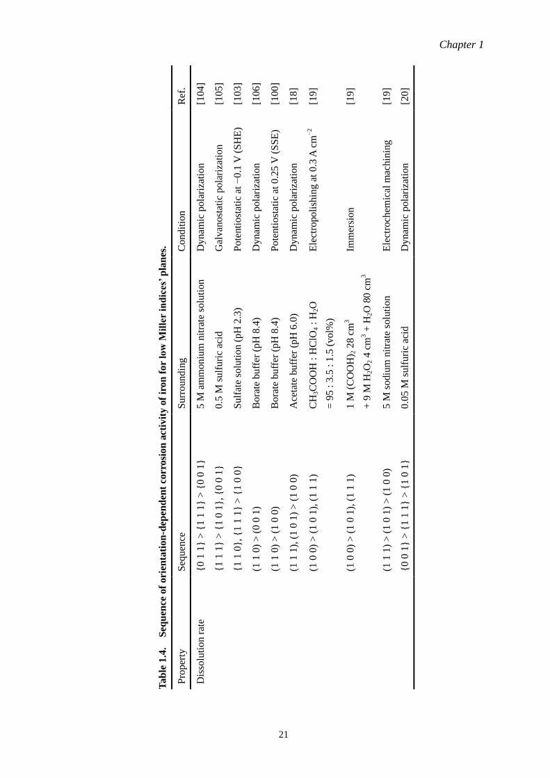
reactions of iron. The orientation-dependent corrosion behavior of iron low Miller indices’ planes
has been reported by several researchers [5,6,17–20,100–106] using single crystals or single
grains on a polycrystalline substrate as sample electrodes. The currently reported corrosion
tendency of the iron planes are summarized in Table 1.4.
The dissolution rate of iron {0 0 1}, {1 0 1}, and {1 1 1} planes has been reported using
several evaluation methods and solutions. Although the sequence shows some scattering, it can be
classified according to the acidity of solution, with the following relation is thought to be a major
suggestion: the dissolution rate becomes larger in the order of {0 0 1} > {1 1 1} > {1 0 1} in
acidic solution and {1 1 1} > {1 0 1} > {0 0 1} in neutral or base solutions. In acidic solution,
Schreiber et al. [19] observed by atomic force microscopy that electropolishing led to the
occurrence of positive, barely visible or step-like grain boundaries on polycrystalline iron,
whereas chemical polishing led to the occurrence of negative and step-like grain boundaries.
Fushimi et al. [20] concluded that the decomposed d-valence charge at the outermost surface
could explain the sequence. For neutral and base solutions, Chiba and Seo [100] explained that
the difference in anodic dissolution rates was due to the surface atom density ρsurf; that of the
{1 0 1} plane is 1.42 times larger than that of the {0 0 1} plane. Schreiber et al. [18] suggested
that electrochemical behavior of three iron planes correlated with ρsurf (Table 1.2); they believed
that the closer distance between the uppermost and second atom layers provided stronger bonding
and resulted in a surface stable against active dissolution.
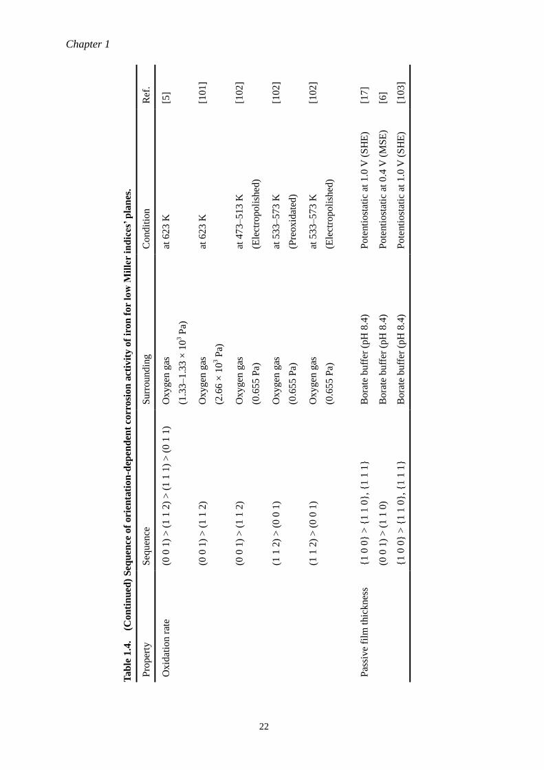
An oxidation rate in air was greatly affected by the substrate structure below 843 K, at
which recrystallization of iron is very slow and FeO does not form due to its thermodynamic
instability [107]. The orientation dependency of the oxidation rate in dry air has been reported at
low oxygen partial pressure and at a temperature range of 473–623 K. Boggs et al. [5] observed
the oxidation behavior of four iron planes and concluded that the formation rate of outer α-Fe2O3
on the surface of inner Fe3O4 reduced the overall oxidation rate, depending on the anisotropic
growth of both oxides. This finding was supported by Ramasubramanian et al. [101]. On the other
hand, Graham and Hussey [102] showed that surface pretreatment greatly affected the oxidation
behavior, rather than the substrate orientation, due to the formation of vacancies that caused a
Chapter 1
20
separation of the metal-oxide interface.
The orientation dependency on the thickness of a passive film on iron single crystals was
reported by Davenport et al. [6], who conducted in situ XRD to identify the detailed structure of
the passive film. The thickness difference was explained by the epitaxial relationship between the
film and the substrate iron. Fushimi et al. [17] observed the heterogeneous thickness of the
passive film formed on polycrystalline iron surface by means of SECM, observing the same grain
dependency as reported by Davenport et al. and indicating that the dependency was caused by ρsurf
of substrate iron and/or the epitaxial relationship between the film and the substrate.
As introduced above, the rough trends of orientation-dependent corrosion of iron have been
clarified. However, the relationship between the crystallographic orientations of an iron surface
and corrosion behavior has not been sufficiently studied, and the detailed mechanism of
orientation-dependent corrosion remains unclear. It is thus necessary to examine
orientation-dependent corrosion behavior in detail and to establish a new corrosion model to
explain it.
1.5. Purpose of this dissertation
As described above, oxide films formed on polycrystalline iron show heterogeneous
behavior and property due to the orientation-dependent corrosion of substrate iron. The
characteristics of the orientation-dependent corrosion of low Miller indices’ iron planes have been
partially studied, but there is still no clear understanding that connects the oxidation behavior and
oxide property of each grain with the heterogeneity of the oxide film formed on whole
polycrystalline substrate. With the aim at connecting them, two measurement techniques were
developed in this dissertation. Micro-electrochemistry with an improved MCC was used to study
the passivation behavior and oxide property of single grains on a polycrystalline iron surface. In
situ 2D ellipsometry was applied to investigate the heterogeneity of the thickness and the
degradation behavior of oxide film formed on whole polycrystalline iron surface. Finally, the
heterogeneity of oxide films formed on polycrystalline iron was discussed from the viewpoints of
both single grains and the whole surface of polycrystalline iron.
Chapter 1
21
Tab
le 1
.4.
S
equ
ence
of
ori
enta
tio
n-d
epen
den
t co
rrosi
on
act
ivit
y o
f ir
on
for
low
Mil
ler
ind
ices
’ p
lan
es.
Ref
.
[10
4]
[10
5]
[10
3]
[10
6]
[10
0]
[18
]
[19
]
[19
]
[19
]
[20
]
Co
nd
itio
n
Dy
nam
ic p
ola
riza
tio
n
Gal
van
ost
atic
pola
riza
tio
n
Po
tenti
ost
atic
at
−0
.1 V
(S
HE
)
Dy
nam
ic p
ola
riza
tio
n
Po
tenti
ost
atic
at
0.2
5 V
(S
SE
)
Dy
nam
ic p
ola
riza
tio
n
Ele
ctro
po
lish
ing
at
0.3
A c
m−
2
Imm
ersi
on
Ele
ctro
chem
ical
mac
hin
ing
Dy
nam
ic p
ola
riza
tio
n
Surr
oundin
g
5 M
am
moniu
m n
itra
te s
olu
tion
0.5
M s
ulf
uri
c ac
id
Sulf
ate
solu
tion
(pH
2.3
)
Bora
te b
uff
er (
pH
8.4
)
Bora
te b
uff
er (
pH
8.4
)
Ace
tate
buff
er (
pH
6.0
)
CH
3C
OO
H :
HC
lO4 :
H2O
= 9
5 :
3.5
: 1
.5 (
vol%
)
1 M
(C
OO
H) 2
28
cm
3
+ 9
M H
2O
2 4
cm
3 +
H2O
80
cm
3
5 M
sodiu
m n
itra
te s
olu
tion
0.0
5 M
sulf
uri
c ac
id
Seq
uen
ce
{0
1 1
} >
{1 1
1} >
{0 0
1}
{1
1 1
} >
{1 0
1},
{0 0
1}
{1
1 0
},
{1 1
1} >
{1 0
0}
(1 1
0)
> (
0 0
1)
(1 1
0)
> (
1 0
0)
(1 1
1),
(1 0
1)
> (
1 0
0)
(1 0
0)
> (
1 0
1),
(1 1
1)
(1 0
0)
> (
1 0
1),
(1 1
1)
(1 1
1)
> (
1 0
1)
> (
1 0
0)
{0
0 1
} >
{1 1
1} >
{1 0
1}
Pro
per
ty
Dis
solu
tio
n r
ate
Chapter 1
22
Tab
le 1
.4.
(C
on
tin
ued
) S
equ
ence
of
ori
enta
tion
-dep
end
ent
corr
osi
on
act
ivit
y o
f ir
on
for
low
Mil
ler
ind
ices
’ p
lan
es.
Ref
.
[5]
[10
1]
[10
2]
[10
2]
[10
2]
[17
]
[6]
[10
3]
Co
nd
itio
n
at 6
23
K
at 6
23
K
at 4
73–5
13 K
(Ele
ctro
poli
shed
)
at 5
33–5
73 K
(Pre
ox
idat
ed)
at 5
33–5
73 K
(Ele
ctro
poli
shed
)
Po
tenti
ost
atic
at
1.0
V (
SH
E)
Po
tenti
ost
atic
at
0.4
V (
MS
E)
Po
tenti
ost
atic
at
1.0
V (
SH
E)
Surr
oundin
g
Oxygen
gas
(1.3
3–1.3
3 ×
10
3 P
a)
Oxygen
gas
(2.6
6 ×
10
3 P
a)
Oxygen
gas
(0.6
55 P
a)
Oxygen
gas
(0.6
55 P
a)
Oxygen
gas
(0.6
55 P
a)
Bora
te b
uff
er (
pH
8.4
)
Bora
te b
uff
er (
pH
8.4
)
Bora
te b
uff
er (
pH
8.4
)
Seq
uen
ce
(0 0
1)
> (
1 1
2)
> (
1 1
1)
> (
0 1
1)
(0 0
1)
> (
1 1
2)
(0 0
1)
> (
1 1
2)
(1 1
2)
> (
0 0
1)
(1 1
2)
> (
0 0
1)
{1
0 0
} >
{1 1
0},
{1 1
1}
(0 0
1)
> (
1 1
0)
{1
0 0
} >
{1 1
0},
{1 1
1}
Pro
per
ty
Oxid
atio
n r
ate
Pas
siv
e fi
lm t
hic
knes
s
Chapter 1
23
References
[1] P. W. Atkins and J. De Paula, Atkins’ Physical Chemistry, 10th Ed., Oxford University Press,
Oxford (2014).
[2] Committee on Cost of Corrosion in Japan, Zairyo-to-Kankyo, 50, 490 (2001).
[3] Z. Xia, Y. Kang, and Q. Wang, J. Magn. Magn. Mater., 320, 3229 (2008).
[4] P. B. Sewell, C. D. Stockbridge, and M. Cohen, J. Electrochem. Soc., 108, 933 (1961).
[5] W. E. Boggs, R. H. Kachik, and G. E. Pellissier, J. Electrochem. Soc., 112, 32 (1967).
[6] A. J. Davenport, L. J. Oblonsky, M. P. Ryan, and M. F. Toney, J. Electrochem. Soc., 147,
2162 (2000).
[7] S. I. Ali and G. C. Wood, Corros. Sci., 8, 413 (1968).
[8] W. Wang and A. Alfantazi, Electrochim. Acta, 131, 79 (2014).
[9] S. Kudelka, A. Michaelis, and J. W. Schultze, Electrochim. Acta, 41, 863 (1996).
[10] D. Abayarathna, E. B. Hale, T. J. O’Keefe, Y.-M. Wang, and D. Radovict, Corros. Sci., 32,
755 (1991).
[11] J. T. Clemens, Bell Labs Techn. J., 2, 76 (1997).
[12] P. Caron and T. Khan, Aerosp. Sci. Technol., 3, 513 (1999).
[13] H. Krawiec and Z. Szklarz, Electrochim. Acta, 203, 426 (2016).
[14] J.-M. Song, Y.-S. Zou, C.-C. Kuo, and S.-C. Lin, Corros. Sci., 74, 223 (2013).
[15] E. Martinez-Lombardia, Y. Gonzalez-Garcia, L. Lapeire, I. De Graeve, K. Verbeken, L.
Kestens, J. M. C. Mol, and H. Terryn, Electrochim. Acta, 116, 89 (2014).
[16] E. Martinez-Lombardia, V. Maurice, L. Lapeire, I. De Graeve, K. Verbeken, L. Kestens, P.
Marcus, and H. Terryn, J. Phys. Chem. C, 118, 25421 (2014).
[17] K. Fushimi, K. Azumi, and M. Seo, ISIJ Int., 39, 346 (1999).
[18] A. Schreiber, J. W. Schultze, M. M. Lohrengel, F. Kármán, and E. Kálmán, Electrochim.
Acta, 51, 2625 (2006).
[19] A. Schreiber, C. Rosenkranz, and M. M. Lohrengel, Electrochim. Acta, 52, 7738 (2007).
[20] K. Fushimi, K. Miyamoto, and H. Konno, Electrochim. Acta, 55, 7322 (2010).
[21] M. Liu, D. Qiu, M.-C. Zhao, G. Song, and A. Atrens, Scr. Mater., 58, 421 (2008).
[22] G.-L. Song and Z. Xu, Corros. Sci., 63, 100 (2012).
[23] K. Fushimi, T. Okawa, K. Azumi, and M. Seo, J. Electrochem. Soc., 147, 524 (2000).
[24] U. König and B. Davepon, Electrochim. Acta, 47, 149 (2001).
[25] M. Hoseini, A. Shahryari, S. Omanovic, and J. A. Szpunar, Corros. Sci., 51, 3064 (2009).
[26] M. Schneider, S. Schroth, J. Schilm, and A. Michaelis, Electrochim. Acta, 54, 2663 (2009).
[27] K. Fushimi, K. Kurauchi, Y. Yamamoto, T. Nakanishi, Y. Hasegawa, and T. Ohtsuka,
Electrochim. Acta, 144, e56 (2014).
[28] C. J. Park, M. M. Lohrengel, T. Hamelmann, M. Pilaski, and H. S. Kwon, Electrochim. Acta,
47, 3395 (2002).
[29] J. W. Schultze, M. Pilaski, M. M. Lohrengel, and U. Konig, Faraday Discuss., 121, 211
Chapter 1
24
(2002).
[30] B. D. B. Aaronson, C.-H. Chen, H. Li, M. T. M. Koper, S. C. S. Lai, and P. R. Unwin, J. Am.
Chem. Soc., 135, 3873 (2013).
[31] World Steel Association, Steel Statistical Yearbook 2016.
[32] The Research Institute of Innovative Technology for the Earth (RITE), 地球環境国際研究
推進事業(脱地球温暖化と持続的発展可能な経済社会実現のための対応戦略の研究)
成果報告書, (2011).
[33] F. W. Clarke and H. S. Washington, The composition of the Earth’s crust, Government
Printing Office, Washington (1924).
[34] H. W. King, in CRC Handbook of Chemistry and Physics, W. M. Haynes and D. R. Lide,
Editors, p. 12–15, CRC Press, New York (2011).
[35] B.-Q. Fu, W. Liu, and Z.-L. Li, Appl. Surf. Sci., 255, 8511 (2009).
[36] J. Radilla, G. E. Negrón-Silva, M. Palomar-Pardavé, M. Romero-Romo, and M. Galván,
Electrochim. Acta, 112, 577 (2013).
[37] P. Błoński and A. Kiejna, Surf. Sci., 601, 123 (2007).
[38] A. J. Bard and L. R. Faulkner, Electrochemical Methods: Fundamentals and Applications,
2nd ed., John Wiley & sons, New York (2001).
[39] U. R. Evans, Metallic Corrosion, Passivity and Protection, E. Arnold & Co., London (1937).
[40] J. O. Bockris, D. Drazic, and A. R. Despic, Electrochim. Acta, 4, 325 (1961).
[41] K. E. Heusler, Berichte der Bunsengesellschaft für Phys. Chemie, 62, 582 (1958).
[42] F. Hibert, Y. Miyoshi, G. Eichkorn, and W. J. Lorenz, J. Electrochem. Soc., 118, 1919
(1971).
[43] F. Hibert, Y. Miyoshi, G. Eichkorn, and W. J. Lorenz, J. Electrochem. Soc., 118, 1927
(1971).
[44] H. Schweickert and W. J. Lorenz, J. Electrochem. Soc., 127, 1693 (1980).
[45] M. Pourbaix, Atlas of Electrochemical Equilibria in Aqueous Solution, 2nd English ed.,
p. 307, National Association of Corrosion Engineers, Houston (1974).
[46] N. Cabrera and N. F. Mott, Rep. Prog. Phys., 12, 163 (1949).
[47] G. T. Burstein and A. J. Davenport, J. Electrochem. Soc., 136, 936 (1989).
[48] C. Y. Chao, L. F. Lin, and D. D. Macdonald, J. Electrochem. Soc., 128, 1187 (1981).
[49] D. D. MacDonald, Electrochim. Acta, 56, 1761 (2011).
[50] M. Nagayama and M. Cohen, J. Electrochem. Soc., 109, 781 (1962).
[51] K. Kuroda, B. D. Cahan, G. Nazri, E. Yeager, and T. E. Mitchell, J. Electrochem. Soc., 129,
2163 (1982).
[52] N. Sato, K. Kudo, and R. Nishimura, J. Electrochem. Soc., 123, 1419 (1976).
[53] S. C. Tjong and E. Yeager, J. Electrochem. Soc., 128, 2251 (1981).
[54] L. J. Oblonsky and T. M. Devine, Corros. Sci., 37, 17 (1995).
[55] L. J. Oblonsky, S. Virtanen, V. Schroeder, and T. M. Devine, J. Electrochem. Soc., 144,
Chapter 1
25
1604 (1997).
[56] V. Schroeder, J. Electrochem. Soc., 146, 4061 (1999).
[57] A. J. Davenport and M. Sansone, J. Electrochem. Soc., 142, 725 (1995).
[58] A. J. Davenport, J. A. Bardwell, and C. M. Vitus, J. Electrochem. Soc., 142, 721 (1995).
[59] P. Schmuki, J. Electrochem. Soc., 143, 574 (1996).
[60] M. P. Ryan, R. C. Newman, and G. E. Thompson, J. Electrochem. Soc., 142, L177 (1995).
[61] E. E. Rees, M. P. Ryan, and D. S. McPhail, Electrochem. Solid-State Lett., 5, B21 (2002).
[62] Y. Mori, M. Hashimoto, and J. Liao, ISIJ Int., 53, 1057 (2013).
[63] C. Zhang, Z.-W. Zhang, and L. Liu, Electrochim. Acta, 210, 401 (2016).
[64] N. Sato and G. Okamoto, in Comprehensive Treatise of Electrochemistry Vol. 4:
Electrochemical Materials Science, J. O. M. Bockris, B. E. Conway, E. Yeager, and R. E.
White, Editors, p. 193, Plenum Press, New York and London (1981).
[65] R. Nishimura and N. Sato, ISIJ Int., 31, 177 (1991).
[66] I. V. Sieber, H. Hildebrand, S. Virtanen, and P. Schmuki, Corros. Sci., 48, 3472 (2006).
[67] H. Deng, H. Nanjo, P. Qian, A. Santosa, I. Ishikawa, and Y. Kurata, Electrochim. Acta, 52,
4272 (2007).
[68] K. Azumi, T. Ohtsuka, and N. Sato, Trans. Jpn. Inst. Met., 27, 382 (1986).
[69] T. Yamamoto, K. Fushimi, S. Miura, and H. Konno, J. Electrochem. Soc., 157, C231 (2010).
[70] K. Azumi, T. Ohtsuka, and N. Sato, J. Electrochem. Soc., 134, 1352 (1987).
[71] E. B. Castro and J. R. Vilche, Electrochim. Acta, 38, 1567 (1993).
[72] M. Buchler, P. Schmuki, H. Böhni, T. Stenberg, and T. Mäntylä, J. Electrochem. Soc., 145,
378 (1998).
[73] Ž. Petrović, M. Metikoš-Huković, and R. Babi, Electrochim. Acta, 75, 406 (2012).
[74] S. Hendy, B. Walker, N. Laycock, and M. Ryan, Phys. Rev. B, 67, 85407 (2003).
[75] S. C. Hendy, N. J. Laycock, and M. P. Ryan, J. Electrochem. Soc., 152, B271 (2005).
[76] C. Albu, S. Van Damme, L. C. Abodi, A. S. Demeter, J. Deconinck, and V. Topa,
Electrochim. Acta, 67, 119 (2012).
[77] K. Asami and K. Hashimoto, Corros. Sci., 17, 559 (1977).
[78] E. McCafferty, M. K. Bernett, and J. S. Murday, Corros. Sci., 28, 559 (1988).
[79] J. Banas, B. Mazurkiewicz, and B. Stypuła, Electrochim. Acta, 37, 1069 (1992).
[80] S. Suzuki, Y. Ishikawa, M. Isshiki, and Y. Waseda, Mater. Trans., 38, 1004 (1997).
[81] L. A. Toledo-Matos and M. A. Pech-Canul, J. Solid State Electrochem., 15, 1927 (2011).
[82] P. Keller and H.-H. Strehblow, Corros. Sci., 46, 1939 (2004).
[83] R.-H. Jung, H. Tsuchiya, and S. Fujimoto, Corros. Sci., 58, 62 (2012).
[84] J.-S. Lee, Y. Kitagawa, T. Nakanishi, Y. Hasegawa, and K. Fushimi, J. Electrochem. Soc.,
162, C685 (2015).
[85] M. Seo, M. Sato, J. B. Lumsden, and R. W. Staehle, Corros. Sci., 17, 209 (1977).
[86] T. Ohtsuka, Mater. Trans., 37, 67 (1996).

Chapter 1
26
[87] M. López-López, J. L. Ferrando, and C. García-Ruiz, Anal. Chem., 85, 2595 (2013).
[88] N. Sato, K. Kudo, and T. Noda, Corros. Sci., 10, 785 (1970).
[89] S. H. Kim, W.-K. Paik, and J. O’M. Bockris, Surf. Sci., 33, 617 (1972).
[90] T. Ohtsuka, M. Masuda, and N. Sato, J. Electrochem. Soc., 132, 787 (1985).
[91] V. Goossens, J. Wielant, S. Van Gils, R. Finsy, and H. Terryn, Surf. Interface Anal., 38, 489
(2006).
[92] N. Sato and K. Kudo, Electrochim. Acta, 16, 447 (1971).
[93] R. Nishimura, K. Kudo, and N. Sato, Surf. Sci., 96, 413 (1980).
[94] A. Furchner, G. Sun, H. Ketelsen, J. Rappich, and K. Hinrichs, Analyst, 140, 1791 (2015).
[95] D. C. Look, K. D. Leedy, and D. L. Agresta, Appl. Phys. Lett., 104, 242107 (2014).
[96] A. J. Bard, F.-R. F. Fan, J. Kwak, and O. Lev, Anal. Chem., 61, 132 (1989).
[97] A. J. Bard, F.-R. F. Fan, D. T. Pierce, P. R. Unwin, D. O. Wipf, and F. Zhou, Science, 254,
68 (1991).
[98] H. Böhni, T. Suter, and A. Schreyer, Electrochim. Acta, 40, 1361 (1995).
[99] M. M. Lohrengel, Electrochim. Acta, 42, 3265 (1997).
[100] M. Chiba and M. Seo, J. Electorchemical Soc., 150, B525 (2003).
[101] N. Ramasubramanian, P. B. Sewell, and M. Cohen, J. Electrochem. Soc., 115, 12 (1968).
[102] M. J. Graham and R. J. Hussey, Oxid. Met., 15, 407 (1981).
[103] K. Fushimi and M. Seo, Electrochim. Acta, 47, 121 (2001).
[104] J. Mieluch and M. Smialowski, Corros. Sci., 4, 237 (1964).
[105] G. P. Cammarota, L. Felloni, G. Palombarini, and S. Sostero Traverso, Corrosion, 129, 129
(1970).
[106] M. Seo and M. Chiba, Electrochim. Acta, 47, 319 (2001).
[107] R. Y. Chen and W. Y. D. Yuen, Oxid. Met., 59, 433 (2003).
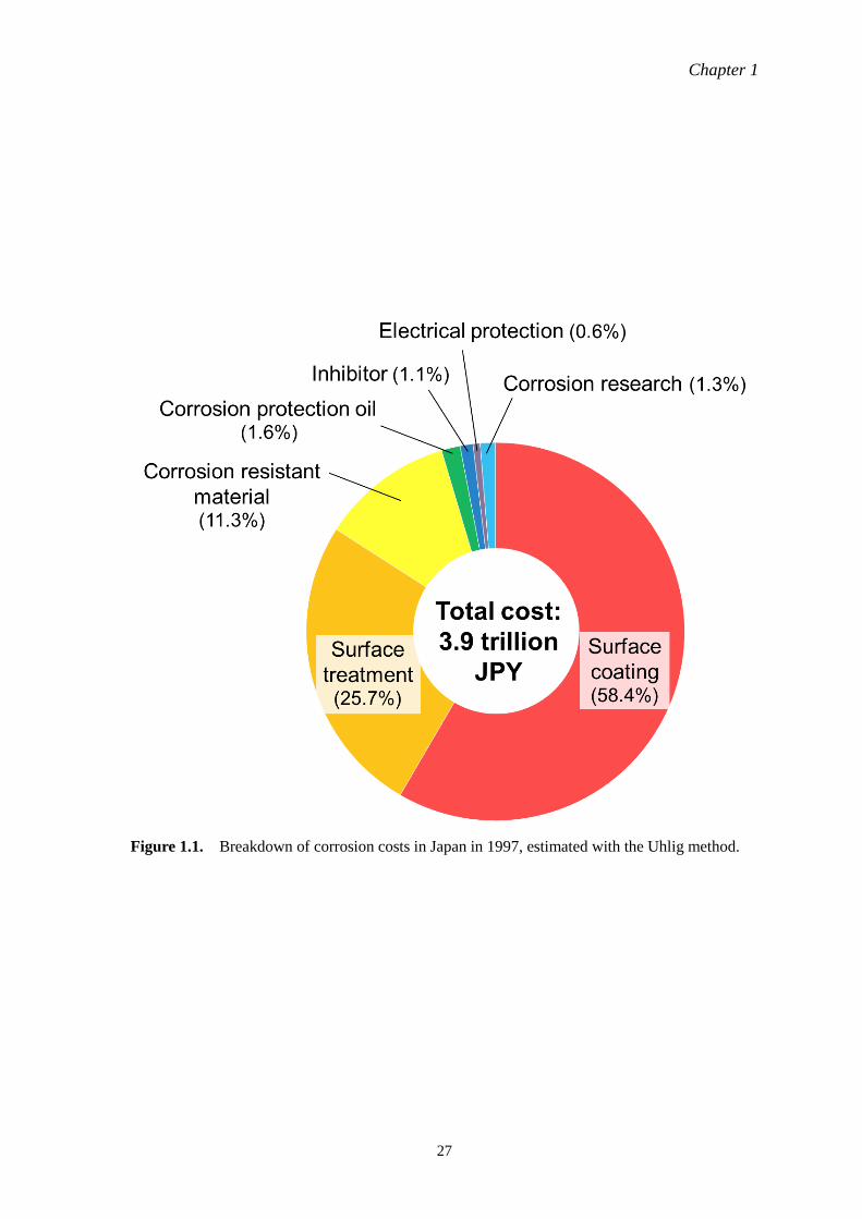
Chapter 1
27
Figure 1.1. Breakdown of corrosion costs in Japan in 1997, estimated with the Uhlig method.
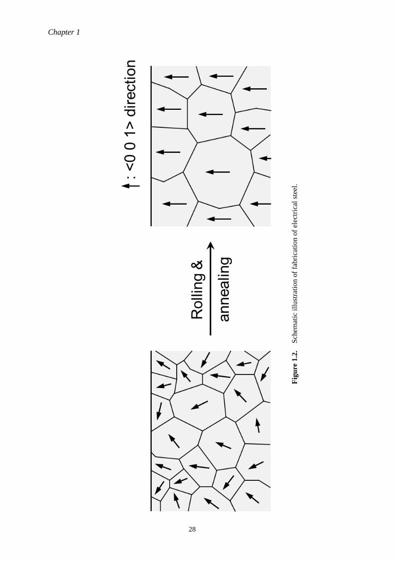
Chapter 1
28
Fig
ure
1.2
. S
chem
atic
ill
ust
rati
on o
f fa
bri
cati
on o
f el
ectr
ical
ste
el.
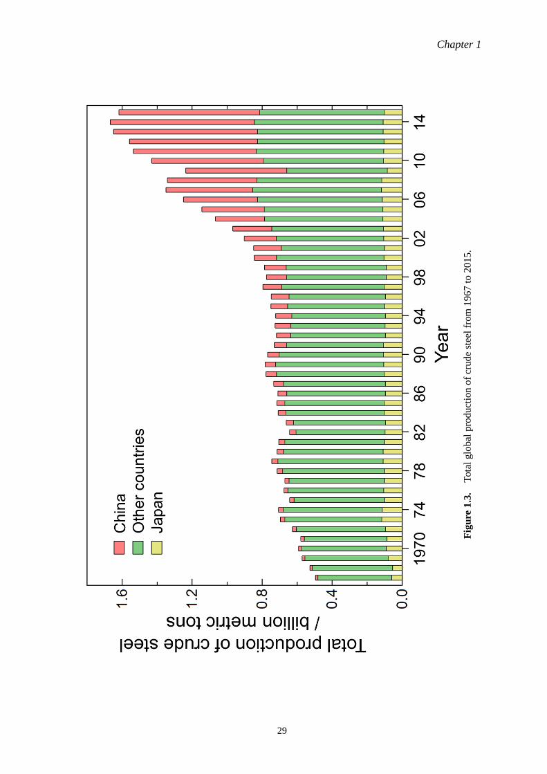
Chapter 1
29
Fig
ure
1.3
. T
ota
l glo
bal
pro
duct
ion
of
crud
e st
eel
from
1967 t
o 2
015.
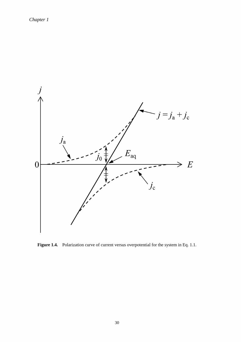
Chapter 1
30
Figure 1.4. Polarization curve of current versus overpotential for the system in Eq. 1.1.
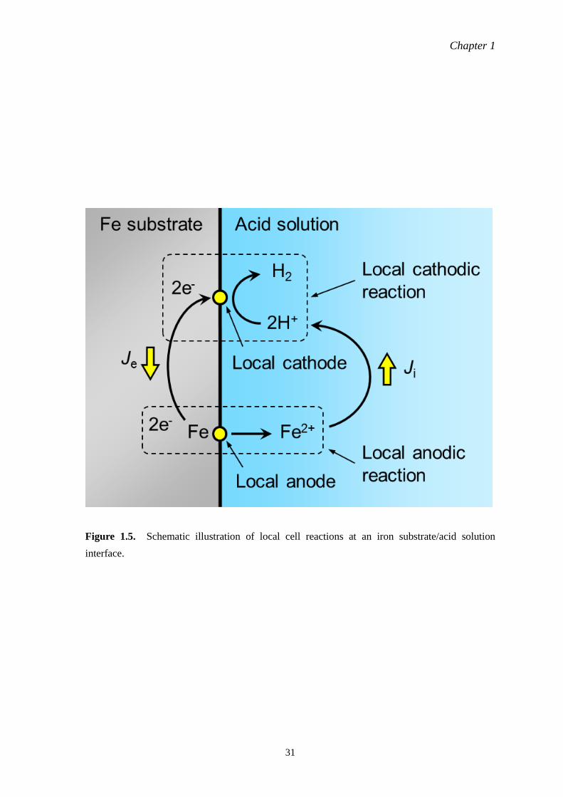
Chapter 1
31
Figure 1.5. Schematic illustration of local cell reactions at an iron substrate/acid solution
interface.
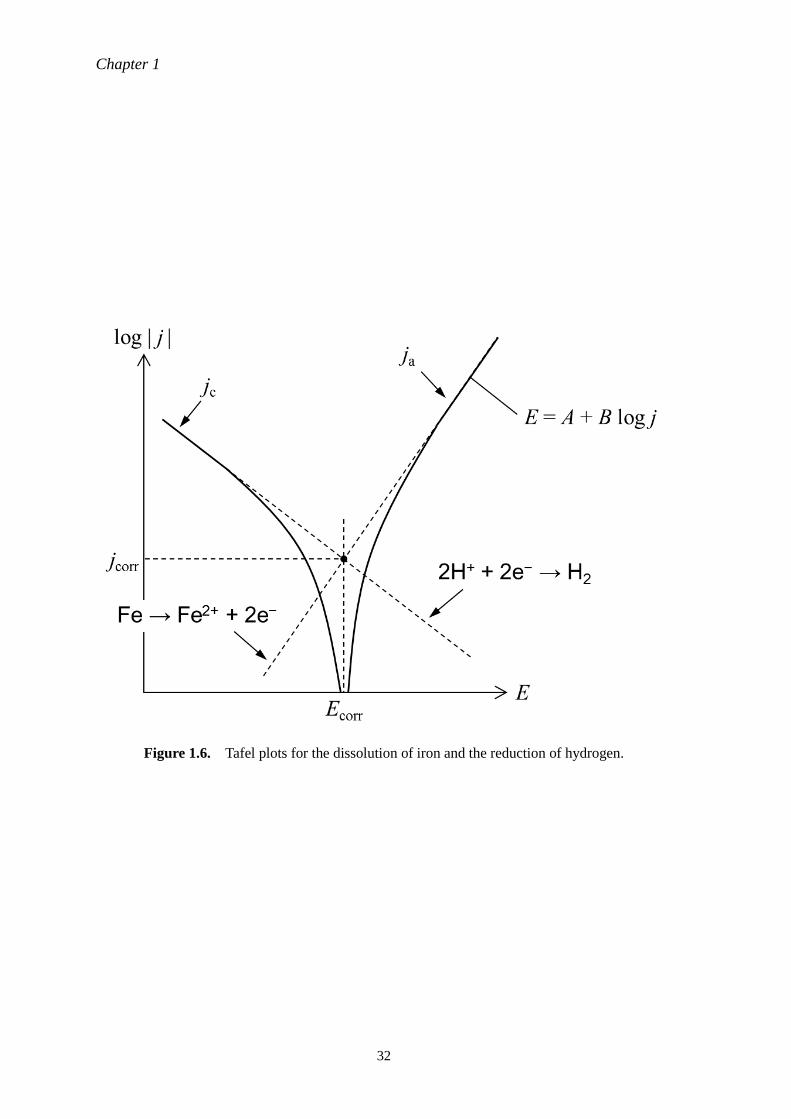
Chapter 1
32
Figure 1.6. Tafel plots for the dissolution of iron and the reduction of hydrogen.
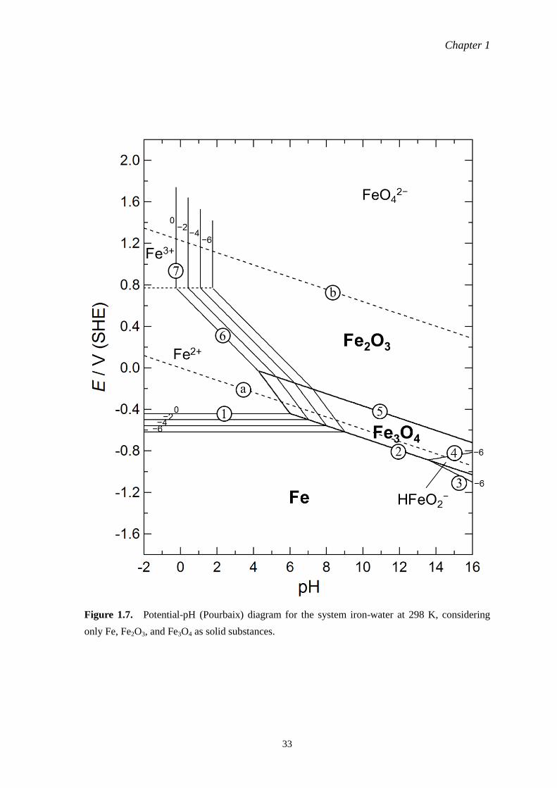
Chapter 1
33
Figure 1.7. Potential-pH (Pourbaix) diagram for the system iron-water at 298 K, considering
only Fe, Fe2O3, and Fe3O4 as solid substances.
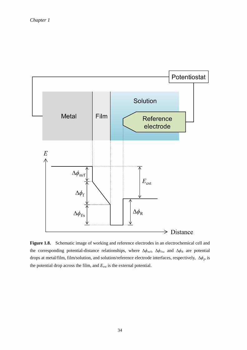
Chapter 1
34
Figure 1.8. Schematic image of working and reference electrodes in an electrochemical cell and
the corresponding potential-distance relationships, where ∆ϕm/f, ∆ϕf/s, and ∆ϕR are potential
drops at metal/film, film/solution, and solution/reference electrode interfaces, respectively, ∆ϕf, is
the potential drop across the film, and Eext is the external potential.
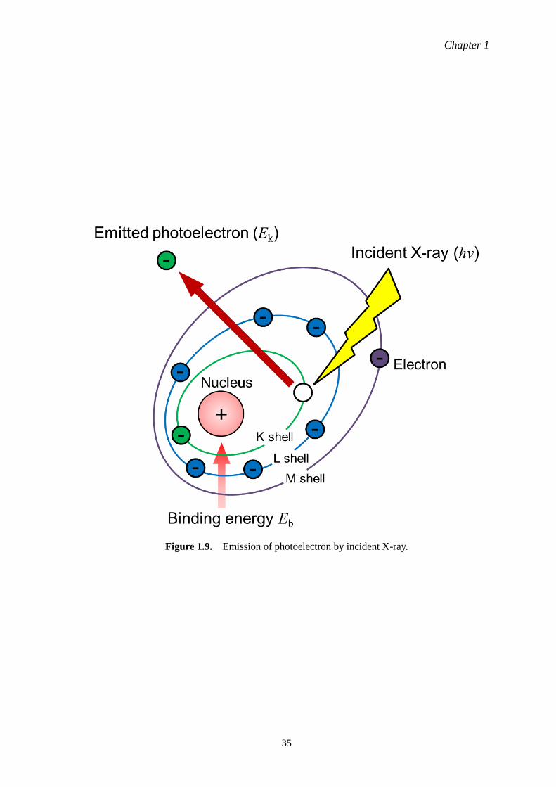
Chapter 1
35
Figure 1.9. Emission of photoelectron by incident X-ray.
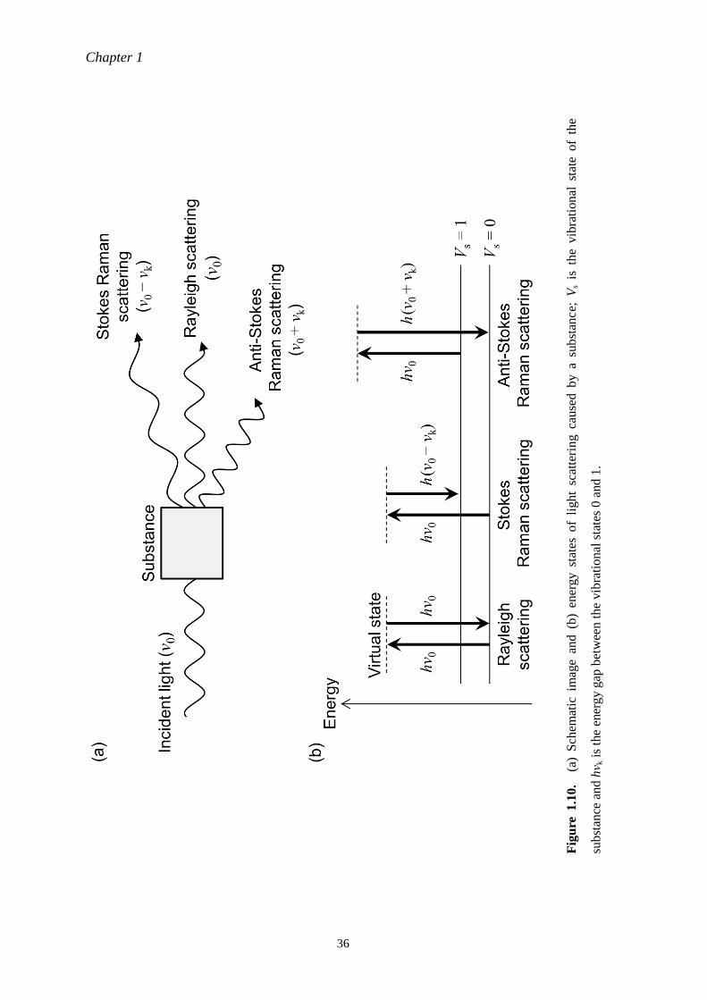
Chapter 1
36
Fig
ure
1.1
0.
(a
) S
chem
atic
im
age
and (
b)
ener
gy s
tate
s of
light
scat
teri
ng c
ause
d b
y a
sub
stan
ce;
Vs
is t
he
vib
rati
on
al s
tate
of
the
sub
stan
ce a
nd
hν k
is
the
ener
gy g
ap b
etw
een t
he
vib
rati
onal
sta
tes
0 a
nd 1
.
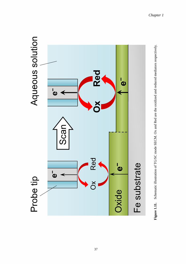
Chapter 1
37
Fig
ure
1.1
1.
S
chem
atic
ill
ust
rati
on o
f T
G/S
C m
ode
SE
CM
. O
x a
nd R
ed a
re t
he
oxid
ized
an
d r
educe
d m
edia
tors
res
pec
tivel
y.
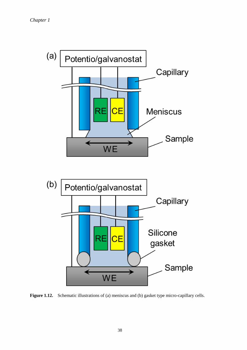
Chapter 1
38
Figure 1.12. Schematic illustrations of (a) meniscus and (b) gasket type micro-capillary cells.
Chapter 2
39
Chapter 2
Experimental techniques and
setups
2.1. Sample preparation
The sample used in this study was a polycrystalline iron plate (purity: 99.99%) provided by
Nippon Steel and Sumitomo Metal corporation. The sample was cut into small pieces (10 mm × 5
mm × 2 mm) by a refine saw (RCO-961, Refinetec) and subjected to the following treatments.
2.1.1. Grain coarsening
When a metal undergoes plastic deformation by rolling processes, dislocations and lattice
defects are induced inside the metal. Since metals and alloys with a distorted lattice structure have
higher strain energy than a well-ordered lattice structure, the former are thermodynamically
unstable and show different reaction behaviors than the latter. Distortion in metals should be
removed for the precise investigation of corrosion behavior, since the atomic arrangement of a
metal surface affects corrosion behavior. For the purpose of releasing lattice distortion and
coarsening crystal grains, the annealing of a sample specimen was performed.
The sample iron pieces were vacuum-encapsulated into a quartz glass tube to avoid
contamination by oxygen and inserted into a tubular furnace. Figure 2.1 shows the sequence of
the annealing. At first, the sample was heated to 1253 K for 3 h and kept at that temperature for 1
h; it was then cooled to 603 K for 48 h. The transformation point of iron from α-phase to γ-phase
is at 1185 K (Table 1.1). This process of crossing the transformation point introduces lattice
disarrangement to the sample as a driving force for the growth of crystal grains. It is known that
the correct temperature for the growth of crystal grains is about approximately one-third to
one-half of the melting point (degrees K basis) of metals [1], or 603–904 K for iron. The
following procedure was then repeated three times: the sample was heated to 1053 K for 4 h, kept
there for 2 h, and cooled to 603 K for 24 h. Finally, the sample was cooled to room temperature.
The upper temperature limit at 1053 K was set to take into account the temperature difference
between the sample and a thermocouple in the furnace.
2.1.2. Surface polishing
The sample specimen was mounted in acrylic resin (Technovit 5071, Heraeus Kulzer) and
Chapter 2
40
ground with the conditions in Table 2.1 by using an auto-grinding machine (LaboForce-3, Struers).
After mirror-like polishing with colloidal SiO2 particles with a diameter of 0.04 µm, the sample
was etched in 10 vol% HNO3 ethanol solution for 10 s to remove the mechanically damaged layer
generated by rough grinding processes. Then, the sample was polished again with the colloidal
silica particles to make the roughened sample surface flat and washed ultrasonically in distilled
water for 60 s. Finally the sample was removed from the resin by breaking it mechanically and
washed ultrasonically in each of acetone and ethanol for 60 s.
Table 2.1. Conditions of mechanical polishing for a sample specimen. Tap water was used
as lubricant for all processes.
Order 1 2 3 4 5
Abrasive MD-Piano 220* SiC-paper SiC-paper SiC-paper MD-chem*
Particle Diamonds SiC SiC SiC SiO2
Grit - #800 #1500 #4000 0.04 µm
Rotating rate (rpm) 300 150 150 150 150
Applied force (N) 30 10 10 10 15
Time (s) to be flat 180 300 420 180
*Abrasive disc produced by Struers
2.1.3. Identification of surface crystallographic orientation
The crystallographic orientation of a polycrystalline iron surface was identified by electron
backscattering diffraction (EBSD) patterning, which is a surface characterization technique to
study the metallographic structure, crystallographic orientation, and phase of crystalline materials.
When an electron beam is incident to a sample tilted 70 degrees in the chamber of a scanning
electron microscope (SEM), an electron diffraction pattern called the Kikuchi pattern is projected
on a phosphor screen serving as a detector (Fig. 2.2). The crystallographic orientation of the
sample surface is determined by indexing pattern bands projected on the screen. Since the escape
depth of diffracted electrons is about 50 nm depending on the measurement conditions, such as
the acceleration voltage and atomic number of a sample, it is important for accurate patterning to
prepare a flat sample surface without a grinding-affected layer. A crystallographic orientation is
described by three Euler angles (φ1, Φ, φ2) as misorientation angles between crystal and sample
frames (Fig. 2.3). The line of node NCS is defined as the intersection of the xy and XY coordinate
planes. A crystallographic orientation is visually represented by a pole figure and an inverse pole
figure (IPF). When one focuses on a certain crystal plane of a sample, a pole figure provides
helpful information; Fig. 2.4a shows the formation of the pole figure of the {0 0 1} plane of a
sample with cubic crystal symmetry. Intersections between the sphere centered at the sample
lattice and {0 0 1} normal directions (NDs) of the sample are projected on a stereographic
projection plane, which is a pole figure. Figures 2.4b–d indicate that the {0 0 1} plane of the
Chapter 2
41
sample is perpendicular to the sample ND and that other {0 0 1} planes are perpendicular to the
sample rolling direction (RD) and transverse direction (TD). On the other hand, when one focuses
on the crystallographic orientation of a sample surface, an IPF is beneficial for optimizing the
orientation. Figure 2.5a shows the IPF on a stereographic projection plane when the sample
(0 0 1) plane is parallel to the sample ND. Figures 2.5b–c indicate when the {1 2 2} and {1 2 3}
planes are perpendicular to the sample ND and the equivalent planes of a sample with cubic
crystal symmetry can be expressed on the shaded unit triangle. In this study, the crystallographic
orientation of the sample surface was displayed by the colors of the unit triangle (Fig 2.5d).
The crystallographic orientation of a polycrystalline iron specimen was identified by an
EBSD apparatus (SC-200, TSL Solutions) incorporated in a field emission Auger electron
microprobe (JAMP-9500F, JEOL) and measurement software (OIM Data Collection 5.31, TSL
Solutions). The conditions of Kikuchi pattern projection and background subtraction are
summarized in Table 2.2. The crystallographic orientation of the sample surface was collected at a
magnification of ×100 with a scanning step of 10 µm. Obtained orientation images were cleaned
under the cleanup parameters of a grain tolerance angle of 5 degrees and a minimum grain size of
5 pixels, using OIM Analysis 5.31 software (TSL Solutions). Figure 2.6 shows the EBSD IPF map
of a typical polycrystalline iron specimen. The annealed sample consists of many grains with
diameters ranging from a few micrometers to 1 mm. Relatively large grains with approximated
{0 0 1}, {1 0 1}, and {1 1 1} planes within a misorientation angle of 10 degrees were used for
micro-electrochemical measurements as working electrodes.
Table 2.2. Typical conditions of Kikuchi pattern projection and background subtraction
for EBSD measurements.
Acceleration
voltage (kV)
Probe
current (nA)
Working
distance (mm) Gain Black
Exposure
(ms) Flames
20 1 25 −2.0 1.0 7.74 30
2.2. Electrochemical measurements with micro-
capillary cell
There are two types of MCCs, depending to the geometry of a capillary tip/sample
electrode interface, as introduced in 1.3.3. In this study, the gasket type MCC was adopted and
developed to conduct electrochemical measurements with a constant electrode area in which the
scanning of the MCC was not necessary.
2.2.1. Fabrication of micro-capillary
A 10 cm-long Pylex glass tube with inner and outer diameters of 3 and 5 mm respectively
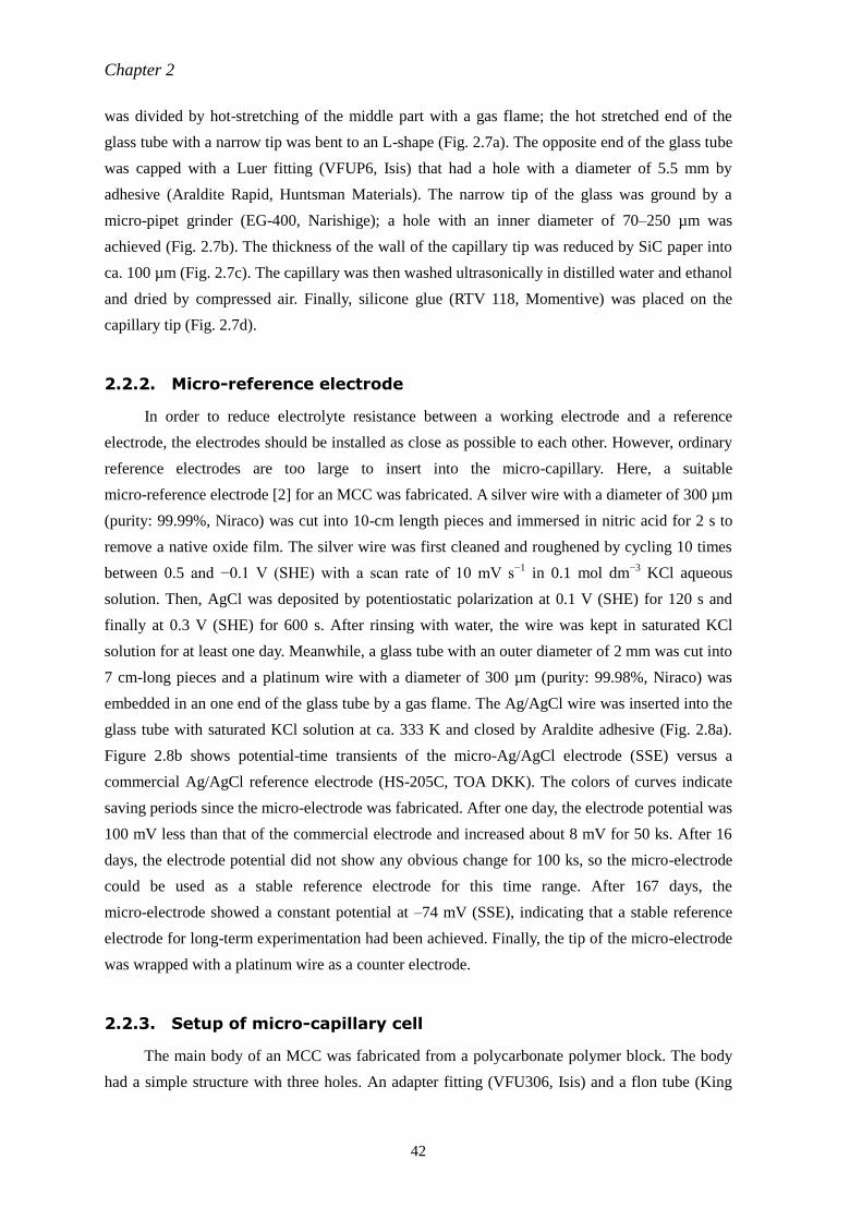
Chapter 2
42
was divided by hot-stretching of the middle part with a gas flame; the hot stretched end of the
glass tube with a narrow tip was bent to an L-shape (Fig. 2.7a). The opposite end of the glass tube
was capped with a Luer fitting (VFUP6, Isis) that had a hole with a diameter of 5.5 mm by
adhesive (Araldite Rapid, Huntsman Materials). The narrow tip of the glass was ground by a
micro-pipet grinder (EG-400, Narishige); a hole with an inner diameter of 70–250 µm was
achieved (Fig. 2.7b). The thickness of the wall of the capillary tip was reduced by SiC paper into
ca. 100 µm (Fig. 2.7c). The capillary was then washed ultrasonically in distilled water and ethanol
and dried by compressed air. Finally, silicone glue (RTV 118, Momentive) was placed on the
capillary tip (Fig. 2.7d).
2.2.2. Micro-reference electrode
In order to reduce electrolyte resistance between a working electrode and a reference
electrode, the electrodes should be installed as close as possible to each other. However, ordinary
reference electrodes are too large to insert into the micro-capillary. Here, a suitable
micro-reference electrode [2] for an MCC was fabricated. A silver wire with a diameter of 300 µm
(purity: 99.99%, Niraco) was cut into 10-cm length pieces and immersed in nitric acid for 2 s to
remove a native oxide film. The silver wire was first cleaned and roughened by cycling 10 times
between 0.5 and −0.1 V (SHE) with a scan rate of 10 mV s−1
in 0.1 mol dm−3
KCl aqueous
solution. Then, AgCl was deposited by potentiostatic polarization at 0.1 V (SHE) for 120 s and
finally at 0.3 V (SHE) for 600 s. After rinsing with water, the wire was kept in saturated KCl
solution for at least one day. Meanwhile, a glass tube with an outer diameter of 2 mm was cut into
7 cm-long pieces and a platinum wire with a diameter of 300 µm (purity: 99.98%, Niraco) was
embedded in an one end of the glass tube by a gas flame. The Ag/AgCl wire was inserted into the
glass tube with saturated KCl solution at ca. 333 K and closed by Araldite adhesive (Fig. 2.8a).
Figure 2.8b shows potential-time transients of the micro-Ag/AgCl electrode (SSE) versus a
commercial Ag/AgCl reference electrode (HS-205C, TOA DKK). The colors of curves indicate
saving periods since the micro-electrode was fabricated. After one day, the electrode potential was
100 mV less than that of the commercial electrode and increased about 8 mV for 50 ks. After 16
days, the electrode potential did not show any obvious change for 100 ks, so the micro-electrode
could be used as a stable reference electrode for this time range. After 167 days, the
micro-electrode showed a constant potential at –74 mV (SSE), indicating that a stable reference
electrode for long-term experimentation had been achieved. Finally, the tip of the micro-electrode
was wrapped with a platinum wire as a counter electrode.
2.2.3. Setup of micro-capillary cell
The main body of an MCC was fabricated from a polycarbonate polymer block. The body
had a simple structure with three holes. An adapter fitting (VFU306, Isis) and a flon tube (King
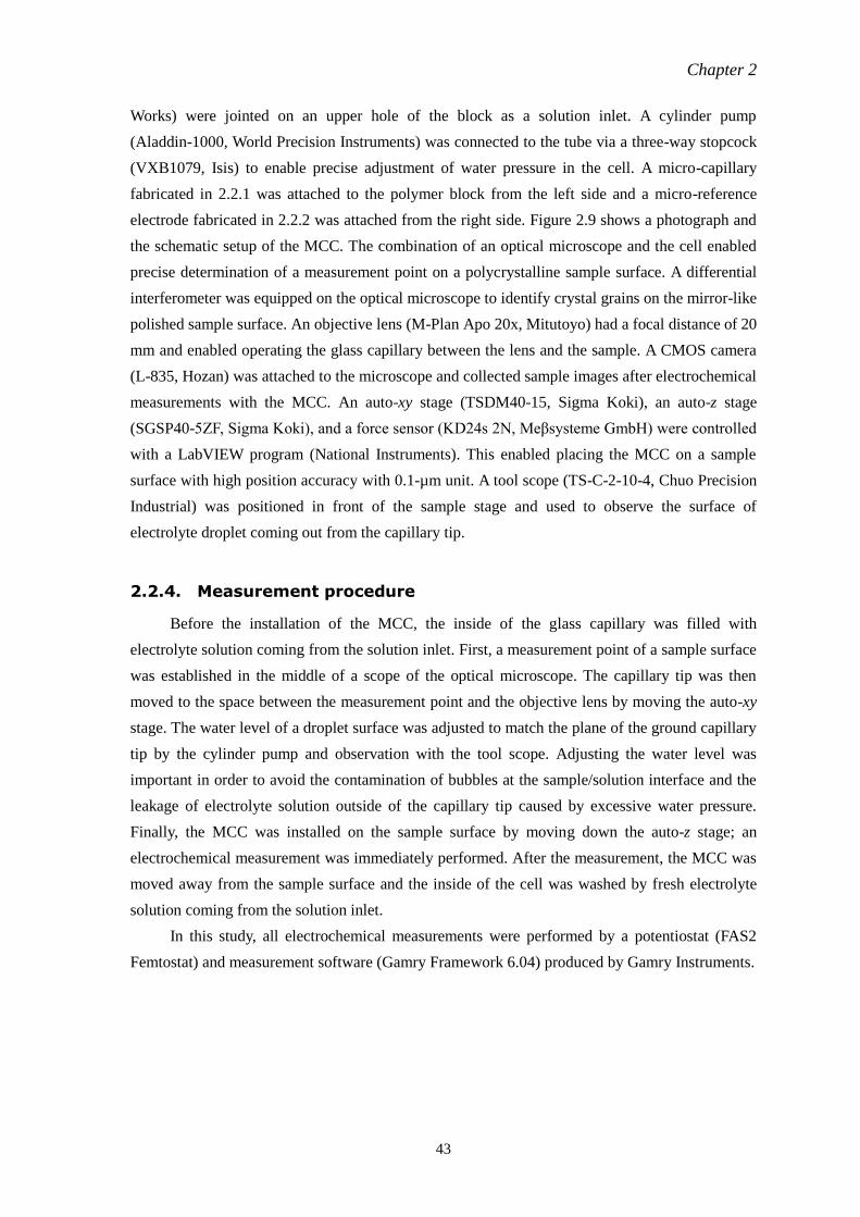
Chapter 2
43
Works) were jointed on an upper hole of the block as a solution inlet. A cylinder pump
(Aladdin-1000, World Precision Instruments) was connected to the tube via a three-way stopcock
(VXB1079, Isis) to enable precise adjustment of water pressure in the cell. A micro-capillary
fabricated in 2.2.1 was attached to the polymer block from the left side and a micro-reference
electrode fabricated in 2.2.2 was attached from the right side. Figure 2.9 shows a photograph and
the schematic setup of the MCC. The combination of an optical microscope and the cell enabled
precise determination of a measurement point on a polycrystalline sample surface. A differential
interferometer was equipped on the optical microscope to identify crystal grains on the mirror-like
polished sample surface. An objective lens (M-Plan Apo 20x, Mitutoyo) had a focal distance of 20
mm and enabled operating the glass capillary between the lens and the sample. A CMOS camera
(L-835, Hozan) was attached to the microscope and collected sample images after electrochemical
measurements with the MCC. An auto-xy stage (TSDM40-15, Sigma Koki), an auto-z stage
(SGSP40-5ZF, Sigma Koki), and a force sensor (KD24s 2N, Meβsysteme GmbH) were controlled
with a LabVIEW program (National Instruments). This enabled placing the MCC on a sample
surface with high position accuracy with 0.1-µm unit. A tool scope (TS-C-2-10-4, Chuo Precision
Industrial) was positioned in front of the sample stage and used to observe the surface of
electrolyte droplet coming out from the capillary tip.
2.2.4. Measurement procedure
Before the installation of the MCC, the inside of the glass capillary was filled with
electrolyte solution coming from the solution inlet. First, a measurement point of a sample surface
was established in the middle of a scope of the optical microscope. The capillary tip was then
moved to the space between the measurement point and the objective lens by moving the auto-xy
stage. The water level of a droplet surface was adjusted to match the plane of the ground capillary
tip by the cylinder pump and observation with the tool scope. Adjusting the water level was
important in order to avoid the contamination of bubbles at the sample/solution interface and the
leakage of electrolyte solution outside of the capillary tip caused by excessive water pressure.
Finally, the MCC was installed on the sample surface by moving down the auto-z stage; an
electrochemical measurement was immediately performed. After the measurement, the MCC was
moved away from the sample surface and the inside of the cell was washed by fresh electrolyte
solution coming from the solution inlet.
In this study, all electrochemical measurements were performed by a potentiostat (FAS2
Femtostat) and measurement software (Gamry Framework 6.04) produced by Gamry Instruments.
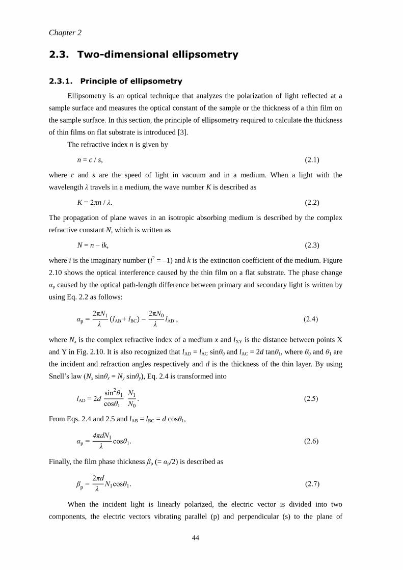
Chapter 2
44
2.3. Two-dimensional ellipsometry
2.3.1. Principle of ellipsometry
Ellipsometry is an optical technique that analyzes the polarization of light reflected at a
sample surface and measures the optical constant of the sample or the thickness of a thin film on
the sample surface. In this section, the principle of ellipsometry required to calculate the thickness
of thin films on flat substrate is introduced [3].
The refractive index n is given by
n = c / s, (2.1)
where c and s are the speed of light in vacuum and in a medium. When a light with the
wavelength λ travels in a medium, the wave number K is described as
K = 2πn / λ. (2.2)
The propagation of plane waves in an isotropic absorbing medium is described by the complex
refractive constant N, which is written as
N = n – ik, (2.3)
where i is the imaginary number (i2 = –1) and k is the extinction coefficient of the medium. Figure
2.10 shows the optical interference caused by the thin film on a flat substrate. The phase change
αp caused by the optical path-length difference between primary and secondary light is written by
using Eq. 2.2 as follows:
αp = 2πN1
λ (lAB + lBC) –
2πN0
λ lAD , (2.4)
where Nx is the complex refractive index of a medium x and lXY is the distance between points X
and Y in Fig. 2.10. It is also recognized that lAD = lAC sinθ0 and lAC = 2d tanθ1, where θ0 and θ1 are
the incident and refraction angles respectively and d is the thickness of the thin layer. By using
Snell’s law (Nx sinθx = Ny sinθy), Eq. 2.4 is transformed into
lAD = 2d sin
2θ1
cosθ1 N1
N0
. (2.5)
From Eqs. 2.4 and 2.5 and lAB = lBC = d cosθ1,
αp = 4πdN1
λ cosθ1. (2.6)
Finally, the film phase thickness βp (= αp/2) is described as
βp =
2πd
λ N1cosθ1. (2.7)
When the incident light is linearly polarized, the electric vector is divided into two
components, the electric vectors vibrating parallel (p) and perpendicular (s) to the plane of
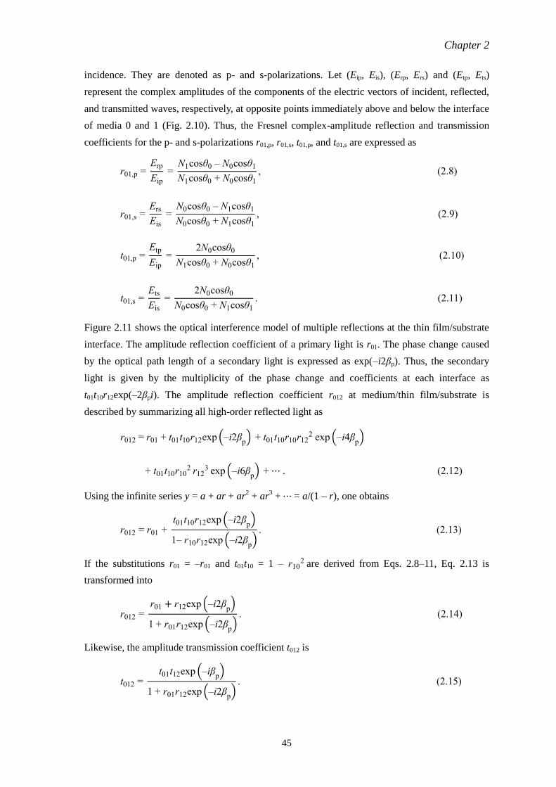
Chapter 2
45
incidence. They are denoted as p- and s-polarizations. Let (Eip, Eis), (Erp, Ers) and (Etp, Ets)
represent the complex amplitudes of the components of the electric vectors of incident, reflected,
and transmitted waves, respectively, at opposite points immediately above and below the interface
of media 0 and 1 (Fig. 2.10). Thus, the Fresnel complex-amplitude reflection and transmission
coefficients for the p- and s-polarizations r01,p, r01,s, t01,p, and t01,s are expressed as
r01,p = Erp
Eip
= N1cosθ0 – N0cosθ1
N1cosθ0 + N0cosθ1
, (2.8)
r01,s = Ers
Eis
= N0cosθ0 – N1cosθ1
N0cosθ0 + N1cosθ1
, (2.9)
t01,p = Etp
Eip
= 2N0cosθ0
N1cosθ0 + N0cosθ1
, (2.10)
t01,s = Ets
Eis
= 2N0cosθ0
N0cosθ0 + N1cosθ1
. (2.11)
Figure 2.11 shows the optical interference model of multiple reflections at the thin film/substrate
interface. The amplitude reflection coefficient of a primary light is r01. The phase change caused
by the optical path length of a secondary light is expressed as exp(–i2βp). Thus, the secondary
light is given by the multiplicity of the phase change and coefficients at each interface as
t01t10r12exp(–2βpi). The amplitude reflection coefficient r012 at medium/thin film/substrate is
described by summarizing all high-order reflected light as
r012 = r01 + t01t10r12exp (–i2βp) + t01t10r10r12
2 exp (–i4βp)
+ t01t10r102 r12
3 exp (–i6βp) + ⋯ . (2.12)
Using the infinite series y = a + ar + ar2 + ar
3 + ⋯ = a/(1 – r), one obtains
r012 = r01 + t01t10r12exp (–i2β
p)
1– r10r12exp (–i2βp)
. (2.13)
If the substitutions r01 = –r01 and t01t10 = 1 – r102 are derived from Eqs. 2.8–11, Eq. 2.13 is
transformed into
r012 = r01 + r12exp (–i2β
p)
1 + r01r12exp (–i2βp)
. (2.14)
Likewise, the amplitude transmission coefficient t012 is
t012 = t01t12exp (–iβ
p)
1 + r01r12exp (–i2βp)
. (2.15)
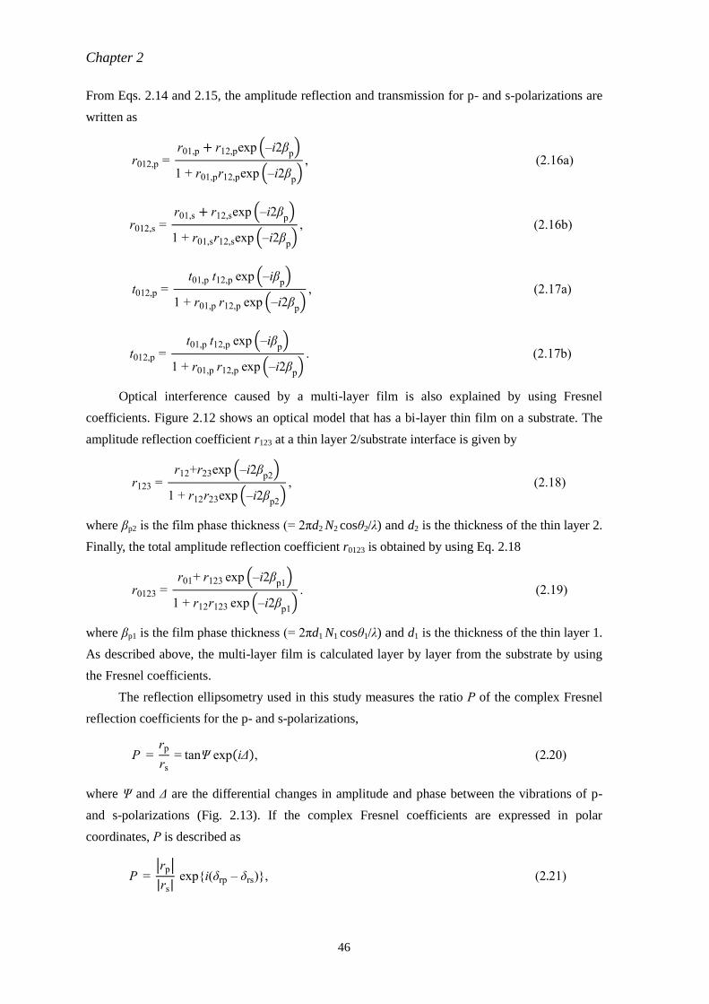
Chapter 2
46
From Eqs. 2.14 and 2.15, the amplitude reflection and transmission for p- and s-polarizations are
written as
r012,p = r01,p + r12,pexp (–i2β
p)
1 + r01,pr12,pexp (–i2βp)
, (2.16a)
r012,s = r01,s + r12,sexp (–i2β
p)
1 + r01,sr12,sexp (–i2βp)
, (2.16b)
t012,p = t01,p t12,p exp (–iβ
p)
1 + r01,p r12,p exp (–i2βp)
, (2.17a)
t012,p = t01,p t12,p exp (–iβ
p)
1 + r01,p r12,p exp (–i2βp)
. (2.17b)
Optical interference caused by a multi-layer film is also explained by using Fresnel
coefficients. Figure 2.12 shows an optical model that has a bi-layer thin film on a substrate. The
amplitude reflection coefficient r123 at a thin layer 2/substrate interface is given by
r123 = r12+r23exp (–i2β
p2)
1 + r12r23exp (–i2βp2
), (2.18)
where βp2 is the film phase thickness (= 2πd2 N2 cosθ2/λ) and d2 is the thickness of the thin layer 2.
Finally, the total amplitude reflection coefficient r0123 is obtained by using Eq. 2.18
r0123 = r01+ r123 exp (–i2β
p1)
1 + r12r123 exp (–i2βp1
). (2.19)
where βp1 is the film phase thickness (= 2πd1 N1 cosθ1/λ) and d1 is the thickness of the thin layer 1.
As described above, the multi-layer film is calculated layer by layer from the substrate by using
the Fresnel coefficients.
The reflection ellipsometry used in this study measures the ratio Ρ of the complex Fresnel
reflection coefficients for the p- and s-polarizations,
Ρ = rp
rs
= tanΨ exp(iΔ), (2.20)
where Ψ and Δ are the differential changes in amplitude and phase between the vibrations of p-
and s-polarizations (Fig. 2.13). If the complex Fresnel coefficients are expressed in polar
coordinates, Ρ is described as
Ρ = |rp|
|rs| exp {i(δrp – δrs)}, (2.21)
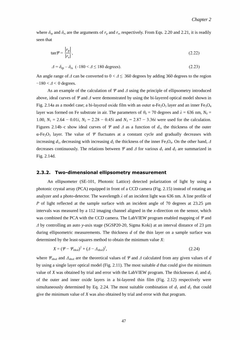
Chapter 2
47
where δrp and δrs are the arguments of rp and rs, respectively. From Eqs. 2.20 and 2.21, it is readily
seen that
tanΨ = |rp|
|rs|, (2.22)
Δ = δrp – δrs (–180 < Δ ≤ 180 degrees). (2.23)
An angle range of Δ can be converted to 0 < Δ ≤ 360 degrees by adding 360 degrees to the region
−180 < Δ < 0 degrees.
As an example of the calculation of Ψ and Δ using the principle of ellipsometry introduced
above, ideal curves of Ψ and Δ were demonstrated by using the bi-layered optical model shown in
Fig. 2.14a as a model case; a bi-layered oxide film with an outer α-Fe2O3 layer and an inner Fe3O4
layer was formed on Fe substrate in air. The parameters of θ0 = 70 degrees and λ = 636 nm, N0 =
1.00, N1 = 2.64 − 0.01i, N2 = 2.28 − 0.45i and N3 = 2.87 − 3.36i were used for the calculation.
Figures 2.14b–c show ideal curves of Ψ and Δ as a function of d1, the thickness of the outer
α-Fe2O3 layer. The value of Ψ fluctuates at a constant cycle and gradually decreases with
increasing d1, decreasing with increasing d2 the thickness of the inner Fe3O4. On the other hand, Δ
decreases continuously. The relations between Ψ and Δ for various d1 and d2 are summarized in
Fig. 2.14d.
2.3.2. Two-dimensional ellipsometry measurement
An ellipsometer (SE-101, Photonic Lattice) detected polarization of light by using a
photonic crystal array (PCA) equipped in front of a CCD camera (Fig. 2.15) instead of rotating an
analyzer and a photo-detector. The wavelength λ of an incident light was 636 nm. A line profile of
Ρ of light reflected at the sample surface with an incident angle of 70 degrees at 23.25 µm
intervals was measured by a 112 imaging channel aligned in the x-direction on the sensor, which
was combined the PCA with the CCD camera. The LabVIEW program enabled mapping of Ψ and
Δ by controlling an auto y-axis stage (SGSP20-20, Sigma Koki) at an interval distance of 23 µm
during ellipsometric measurements. The thickness d of the thin layer on a sample surface was
determined by the least-squares method to obtain the minimum value X:
X = (Ψ − Ψideal)2 + (Δ − Δideal)
2, (2.24)
where Ψideal and Δideal are the theoretical values of Ψ and Δ calculated from any given values of d
by using a single layer optical model (Fig. 2.11). The most suitable d that could give the minimum
value of X was obtained by trial and error with the LabVIEW program. The thicknesses d1 and d2
of the outer and inner oxide layers in a bi-layered thin film (Fig. 2.12) respectively were
simultaneously determined by Eq. 2.24. The most suitable combination of d1 and d2 that could
give the minimum value of X was also obtained by trial and error with that program.
Chapter 2
48
2.3.3. Setup of electrochemical cell for in situ 2D ellipsometry
First, a sample specimen was mounted on an epoxy resin holder with the Araldite Rapid
adhesive. A brass screw in contact with the back side of the sample was used to obtain an electric
contact with the potentiostat. The sample was put in an electrochemical cell designed for in situ
2D ellipsometry, as shown in Fig. 2.16. A platinum wire was used as a counter electrode and an
Ag/AgCl/saturated KCl reference electrode was connected to the cell via a Luggin-Haber
capillary and a salt-bridge of solidified agar with KNO3. The cell was connected with two glass
bottles filled with pH 6.5 and pH 8.4 borate buffer solutions (0.293 mol dm–3
boric acid and
0.00188 mol dm–3
sodium borate, and 0.150 mol dm–3
boric acid and 0.0375 mol dm–3
sodium
borate solutions, respectively.). These solutions were deaerated with bubbling of pure Ar gas and
injected into the cell by the pressure of the Ar gas, thus avoiding the contamination by air of the
cell.
References
[1] 古林英一 著、材料学シリーズ 再結晶と材料組織、内田老鶴圃 (2000).
[2] A. W. Hassel, K. Fushimi, and M. Seo, Electrochem. commun., 1, 180 (1999).
[3] R. M. A. Azzam and N. M. Bashara, Ellipsometry and Polarized Light, p. 269, North-Holland
Personal Library, Amsterdam (1987).
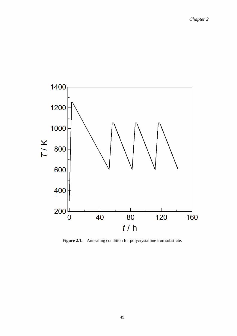
Chapter 2
49
Figure 2.1. Annealing condition for polycrystalline iron substrate.
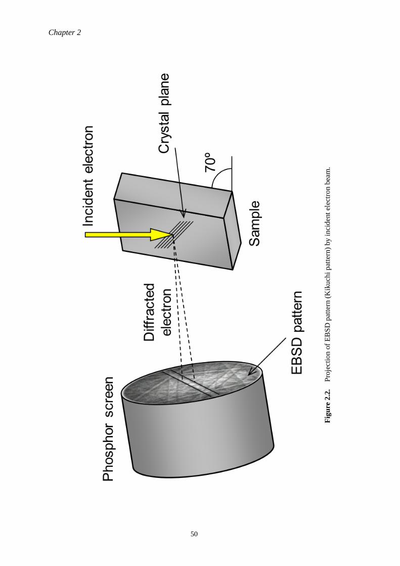
Chapter 2
50
Fig
ure
2.2
. P
roje
ctio
n o
f E
BS
D p
atte
rn (
Kik
uch
i p
atte
rn)
by i
nci
den
t el
ectr
on b
eam
.
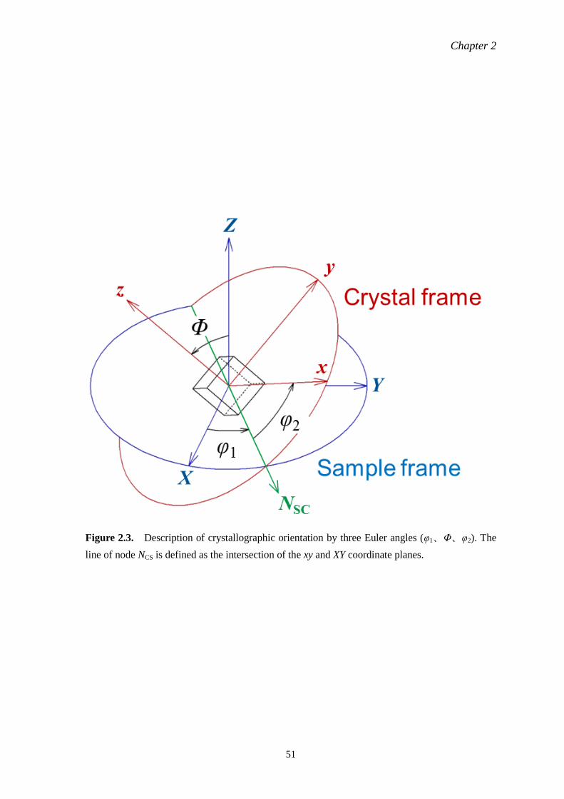
Chapter 2
51
Figure 2.3. Description of crystallographic orientation by three Euler angles (φ1、Φ、φ2). The
line of node NCS is defined as the intersection of the xy and XY coordinate planes.
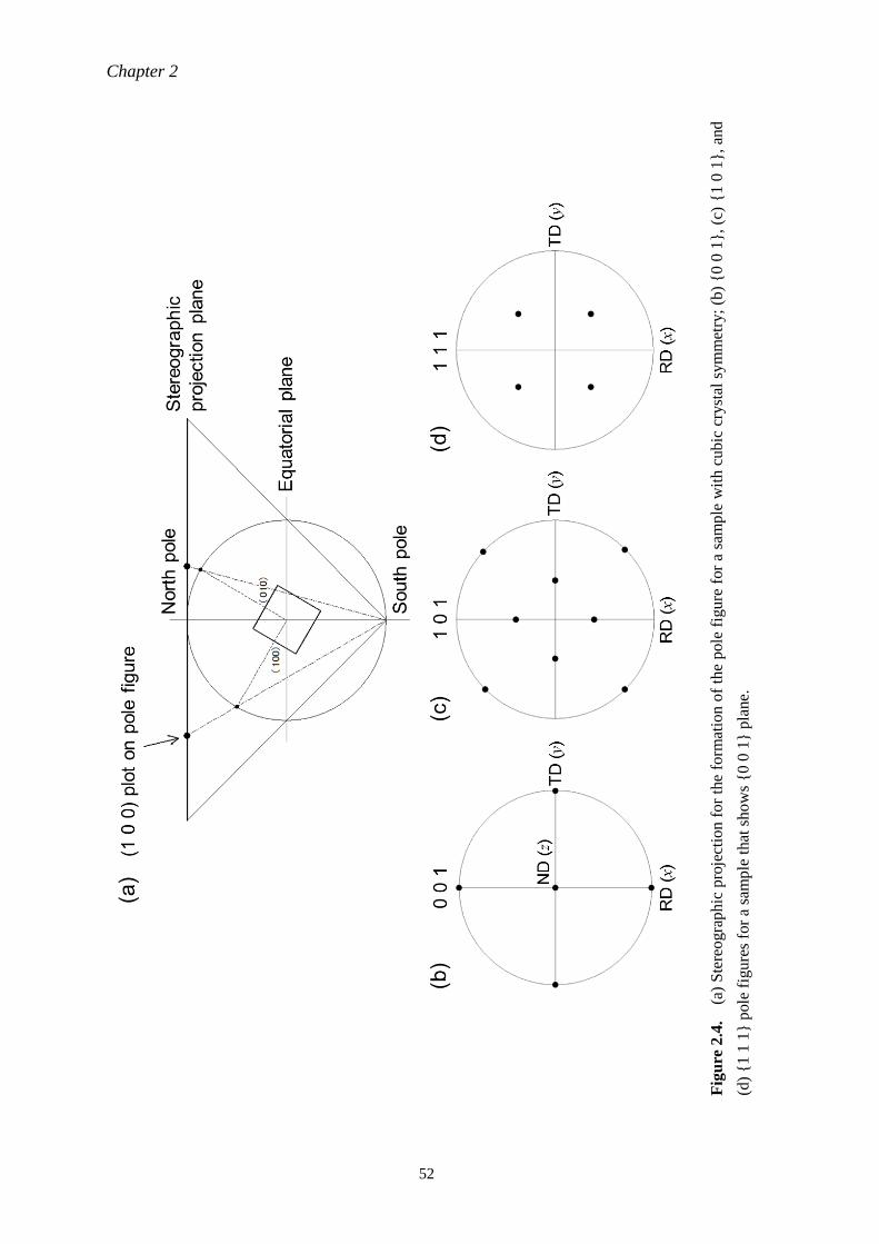
Chapter 2
52
Fig
ure
2.4
.
(a)
Ste
reo
gra
ph
ic p
roje
ctio
n f
or
the
form
atio
n o
f th
e pole
fig
ure
for
a sa
mple
wit
h c
ub
ic c
ryst
al s
ym
met
ry;
(b)
{0
0 1
},
(c)
{1
0 1
},
and
(d)
{1 1
1} p
ole
fig
ure
s fo
r a
sam
ple
that
show
s {0 0
1} p
lane.
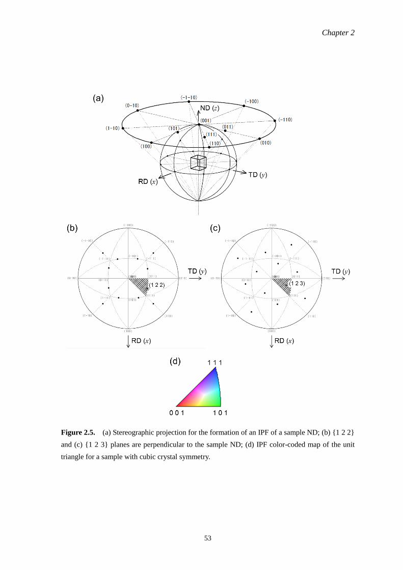
Chapter 2
53
Figure 2.5. (a) Stereographic projection for the formation of an IPF of a sample ND; (b) {1 2 2}
and (c) {1 2 3} planes are perpendicular to the sample ND; (d) IPF color-coded map of the unit
triangle for a sample with cubic crystal symmetry.
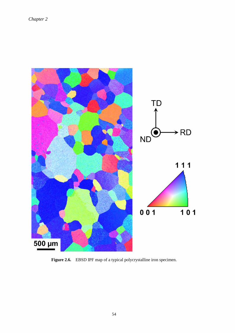
Chapter 2
54
Figure 2.6. EBSD IPF map of a typical polycrystalline iron specimen.
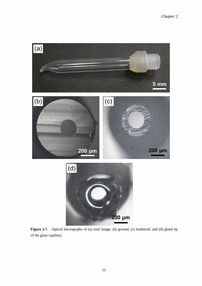
Chapter 2
55
Figure 2.7. Optical micrographs of (a) total image, (b) ground, (c) feathered, and (d) glued tip
of the glass capillary.
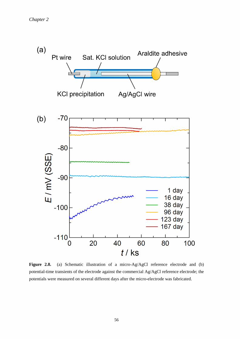
Chapter 2
56
Figure 2.8. (a) Schematic illustration of a micro-Ag/AgCl reference electrode and (b)
potential-time transients of the electrode against the commercial Ag/AgCl reference electrode; the
potentials were measured on several different days after the micro-electrode was fabricated.
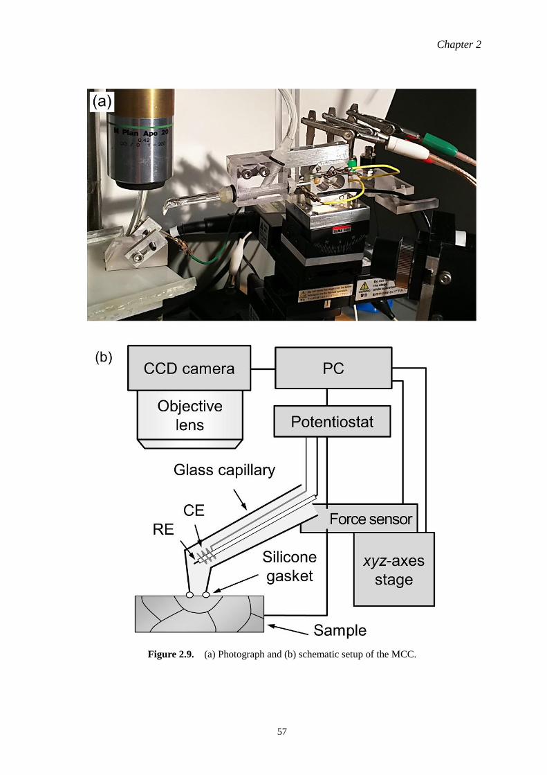
Chapter 2
57
Figure 2.9. (a) Photograph and (b) schematic setup of the MCC.
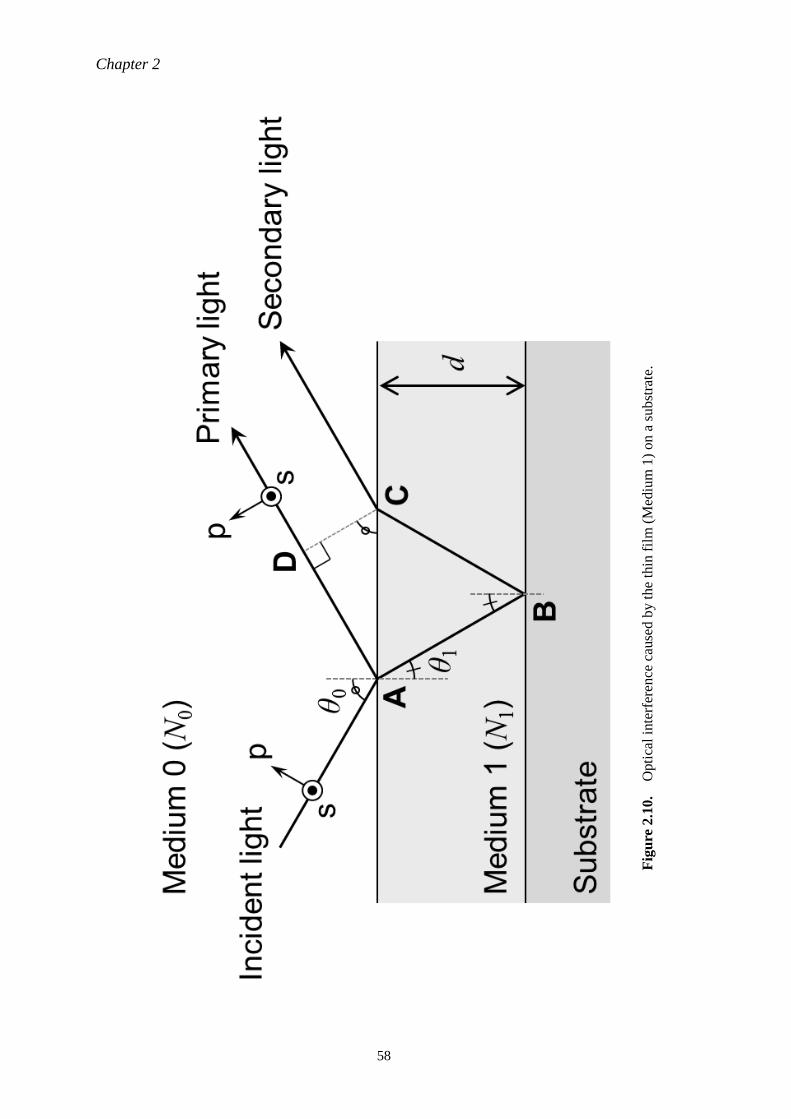
Chapter 2
58
Fig
ure
2.1
0.
O
pti
cal
inte
rfer
ence
cau
sed b
y t
he
thin
fil
m (
Med
ium
1)
on
a s
ub
stra
te.
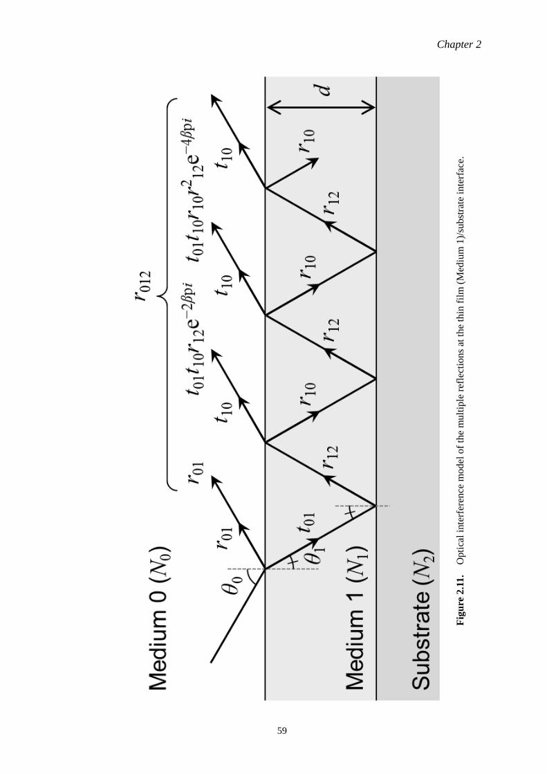
Chapter 2
59
Fig
ure
2.1
1.
O
pti
cal
inte
rfer
ence
model
of
the
mult
iple
ref
lect
ions
at t
he
thin
fil
m (
Med
ium
1)/
subst
rate
in
terf
ace.
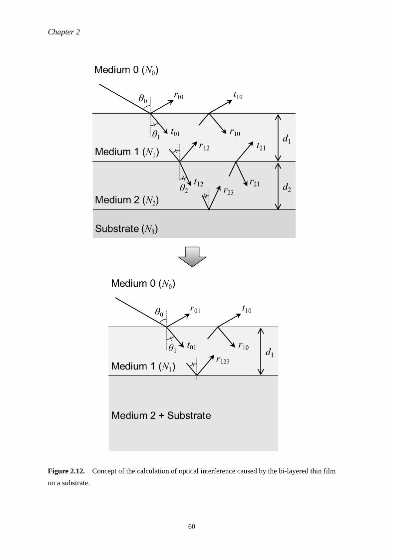
Chapter 2
60
Figure 2.12. Concept of the calculation of optical interference caused by the bi-layered thin film
on a substrate.
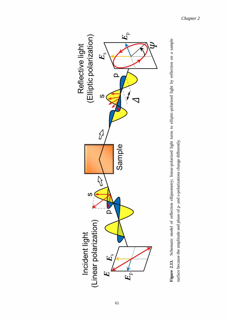
Chapter 2
61
Fig
ure
2.1
3.
S
chem
atic
mo
del
of
refl
ecti
on e
llip
som
etry
; li
nea
r-pola
rize
d l
ight
turn
s to
ell
ipti
c-p
ola
rize
d l
igh
t b
y r
efle
ctio
n o
n a
sam
ple
surf
ace
bec
ause
th
e am
pli
tud
e an
d p
has
e of
p-
and s
-po
lari
zati
ons
chan
ge
dif
fere
ntl
y.
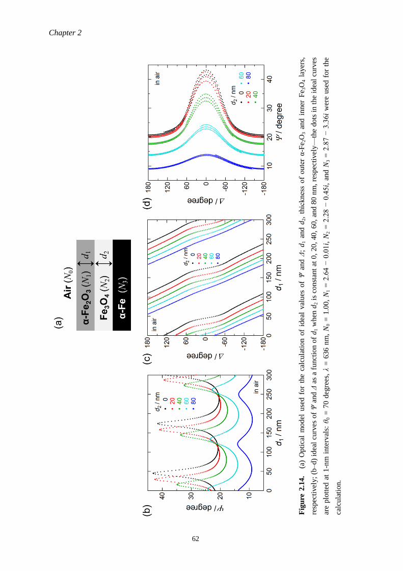
Chapter 2
62
Fig
ure
2.1
4.
(a
) O
pti
cal
mo
del
use
d f
or
the
calc
ula
tion o
f id
eal
val
ues
of
Ψ a
nd Δ
; d
1 a
nd d
2,
thic
kn
ess
of
ou
ter
α-F
e 2O
3 a
nd
in
ner
Fe 3
O4 l
ayer
s,
resp
ecti
vel
y;
(b–d
) id
eal
curv
es o
f Ψ
an
d Δ
as
a fu
nct
ion o
f d
1 w
hen
d2 i
s co
nst
ant
at 0
, 20,
40,
60
, an
d 8
0 n
m,
resp
ecti
vel
y—
the
do
ts i
n t
he
idea
l cu
rves
are
plo
tted
at
1-n
m i
nte
rval
s: θ
0 =
70 d
egre
es,
λ =
636
nm
, N
0 =
1.0
0,
N1 =
2.6
4 −
0.0
1i,
N2 =
2.2
8 −
0.4
5i,
and N
3 =
2.8
7 −
3.3
6i
wer
e use
d f
or
the
calc
ula
tion
.
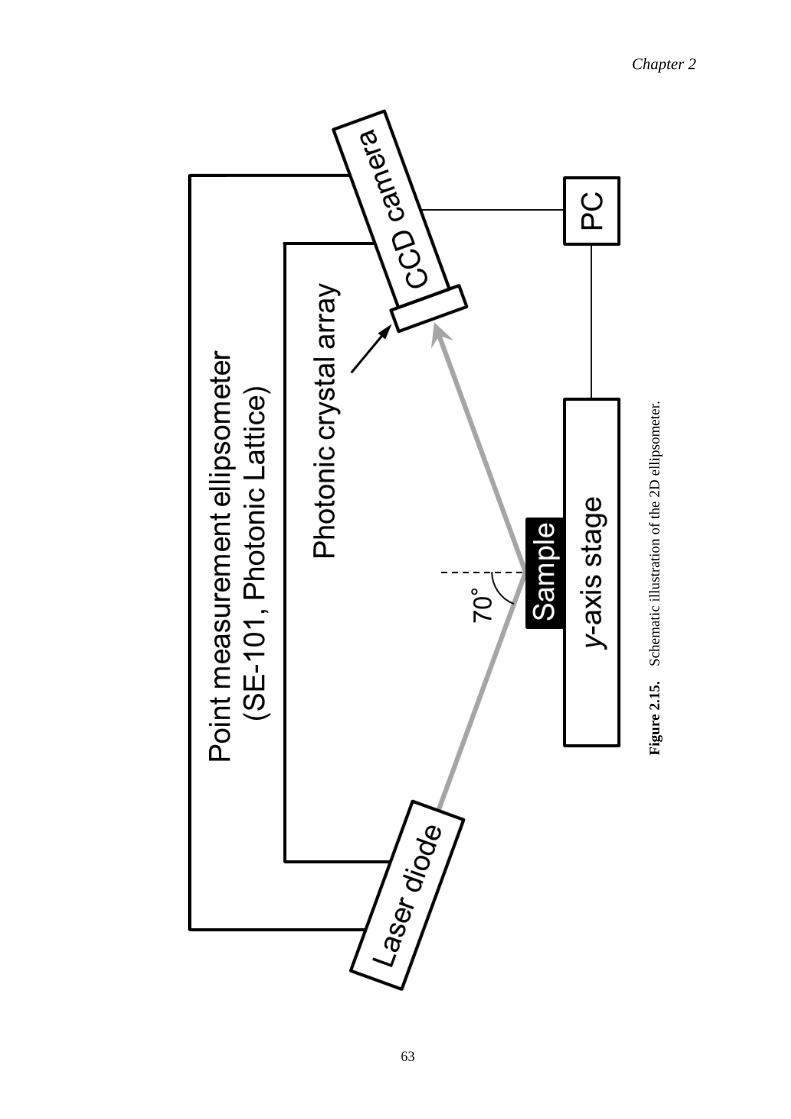
Chapter 2
63
Fig
ure
2.1
5.
S
chem
atic
ill
ust
rati
on o
f th
e 2D
ell
ipso
met
er.
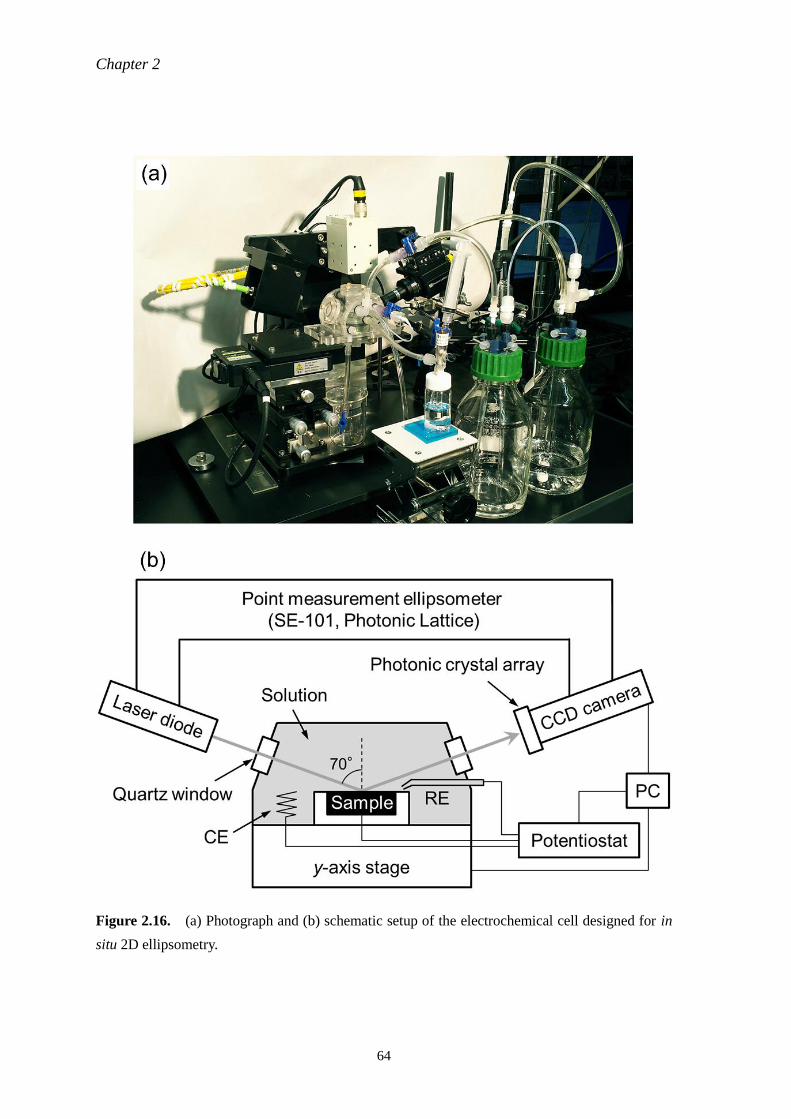
Chapter 2
64
Figure 2.16. (a) Photograph and (b) schematic setup of the electrochemical cell designed for in
situ 2D ellipsometry.
Chapter 3
65
Chapter 3
Grain-dependent oxidation
behavior in sulfuric acid measured
by micro-capillary cell
3.1. Introduction
The polarization behavior of iron depends on the pH of the electrolyte solution [1,2].
Anodic currents in active and passive states increase with decreasing pH. In the passive state, the
anodic current is suppressed by the formation of a passive oxide film and the steady state current
increases with decreasing the solution pH due to the dissolution of iron ions into the solution
through the passive film. The passive film thickness at steady state is a linear function of the
applied potential. Ellipsometric measurement revealed that the structure of the passive film
formed in acid solution was a bi-layered barrier film of inner Fe3O4 and outer γ-Fe2O3, and
photoelectric potential measurements demonstrated the n-type semiconductive property of the
passive oxide.
The orientation-dependent corrosion of iron in acid solution was observed through its
dissolution rate (Table 1.4). The anisotropic dissolution of iron has been examined by means of
several measurement methods by researchers and the tendencies of the dissolution rate have been
clarified. Grain-dependent dissolution of polycrystalline iron was reported by Fushimi and Seo [3],
who conducted SECM in pH 2.3 sulfate solution. In such an environment, it is expected that iron
will also show orientation dependency in passivation behavior; however, there is no published
research that investigated the orientation dependency of the passive film formed in acid solution,
and the mechanism of grain-dependent passivation remains unclear. In order to elucidate the
precise corrosion reaction that occurs on a polycrystalline iron surface, it is necessary to examine
both the passivation behavior and the dissolution behavior of each grain on the polycrystalline
substrate.
In this chapter, the grain-dependent oxidation behavior of iron single grains in sulfuric acid
was investigated using an MCC method in order to reveal how the surface orientation determines
passive film formation.
Chapter 3
66
3.2. Experimental
3.2.1. Micro-electrochemical measurements
Micro-electrochemical measurements were carried out by using the MCC developed in
section 2.2. In this section, three glass capillaries with different tip geometry were used for the
MCC. Figure 3.1 presents optical images of the glass capillaries; their sizes are summarized in
Table 3.1. The tips have different inner diameters and widths of silicone rubber. All potentials
measured versus SSE were converted into potentials versus RHE. The inside of the capillary was
filled with an electrolyte of 0.05 mol dm−3 H2SO4 aqueous solution (pH 1.3), deaerated by
bubbling of pure Ar gas before measurement. Crystal grains for which crystallographic orientation
could be approximated to {0 0 1}, {1 0 1}, and {1 1 1} planes within an Euler angle disparity of
10 degrees were used as sample electrodes.
Table 3.1. Sizes of capillary tips of MCCs; AMCC, achieved electrode area.
No. Inner diameter (µm) Silicone gasket AMCC (cm2) Tip image
C1 93 thick and wide 6.8 × 10⁻⁵
Fig. 3.1a
C2 70 thin and narrow 3.7 × 10⁻⁵
Fig. 3.1b
C3 250 thin and narrow 5.1 × 10⁻⁴
Fig. 3.1c
After Ecorr measurement for 300 s, potentiodynamic polarization was performed from (Ecorr
− 0.1 V) to 1.9 V (RHE) at a potential sweep rate of 5 mV s−1
with the capillary C1 or C2. The
morphology of the sample surface after potentiodynamic polarization was observed with a
field-emission SEM (JSM-6500F, JEOL). On a fresh sample surface, potentiostatic polarization
was carried out at 1.2 V (RHE) for 1 h with the capillary C3 and the current transient was
recorded. Immediately after the potentiostatic polarization, EIS was performed at 1.2 V (RHE)
with an ac voltage amplitude of ±10 mV in a frequency range of 105 to 10
−2 Hz. Curve fitting of
impedance spectrum was done by using a suitable equivalent electronic circuit (EEC) with
analysis software (Echem Analyst 6.04, Gamry Instruments). Furthermore, after the potentiostatic
polarization at 1.2 V (RHE), impedance measurements for MS analysis were conducted in a
potential range from 1.2 to 0.5 V (RHE) with an ac voltage amplitude of ±10 mV at the frequency
of 100 Hz. Separately, the sample polarized at 1.2 V (RHE) for 1 h was galvanostatically reduced
at −6 µA cm−2
[4] and the potential transient of the sample electrode was recorded. All
electrochemical measurements were conducted in an air-conditioned room at 295 K.
3.2.2. X-ray photoelectron spectroscopy
After potentiostatic polarization by the MCC with the capillary C3, the samples were
immediately rinsed with ethanol and dried with clean air. The chemical state of the polarized
Chapter 3
67
sample surface was studied by XPS. Photoelectron spectra were recorded using a JPS-9200
photoelectron spectrometer (JEOL) with Al Kα radiation operating at 100 W (10 kV, 10 mA). This
photoelectron spectrometer can analyze a micro-region by adjusting the angle-limiting aperture
and the field view aperture, which select photoelectrons captured into the electrostatic lens and
the analyzer, instead of focusing an X-ray. Here, we confined the detection area of photoelectrons
to 200 µm in a diameter by adjusting the two apertures to analyze the small sample area polarized
with the MCC. The acquisition of each spectrum was repeated 100 times due to the small
photoelectron intensity obtained from the small detection area. In this study, no sputtering to
remove contamination on the surface was carried out to avoid reduction of oxidized iron species
[5]. Photoelectron spectra were analyzed by using SpecSurf software (JEOL). The C 1s peak from
contaminant carbon at 285.1 eV was used as a reference for charge correction [6]. After
background subtraction using Shirley’s method [7], the spectra were separated into different
oxidation states by deconvolution.
3.3. Results
3.3.1. Corrosion potential and dynamic polarization
Since the diameter of the MCCs was smaller than the grains on the sample, a micro-
electrode could be set on a single grain. Just after the installation of the MCC, the sample surface
showed a relatively noble rest potential; however, it shifted immediately to a steady state value of
Ecorr (Fig. 3.2), suggesting that a native oxide film that had formed on the sample surface was
removed due to the acidity of the electrolyte.
Figure 3.3 shows dynamic polarization curves measured on the iron {0 0 1}, {1 0 1}, and
{1 1 1} grains using the capillary C1. The polarization curves show active, passive, and
trans-passive states of iron. All samples show similar Ecorr values of ca. −0.22 V (RHE), though
this is more positive than previous results [8] obtained in a sufficiently deaerated solution using an
ordinary electrochemical cell. The obscure difference and the positive shift of Ecorr are likely due
to contamination of oxygen dissolved from the tip of the glass capillary before the installation of
the MCC. Compared with ordinary macro-cells, an MCC is sensitive to contamination of the
solution because of its small volume. Regardless of the similar Ecorr values, an anodic current
flowing in the active state from Ecorr to ca. 0.76 V is due to active dissolution and was slightly
dependent on the surface crystallographic orientation. The electric charge qa consumed in the
active state was in the order of {1 1 1} > {1 0 1} > {0 0 1} grains (Table 3.2). Subsequently, a
small current flowed on each grain in the passive state from ca. 0.76 to 1.46 V (RHE), due to
passivation of the surface. The current included fluctuations on the {1 0 1} and {1 1 1} grains but
no fluctuation on the {0 0 1} grain. The electric charge qp consumed in the passive state was also
in the order of {1 1 1} > {1 0 1} > {0 0 1} grains associated with the current fluctuations (Table
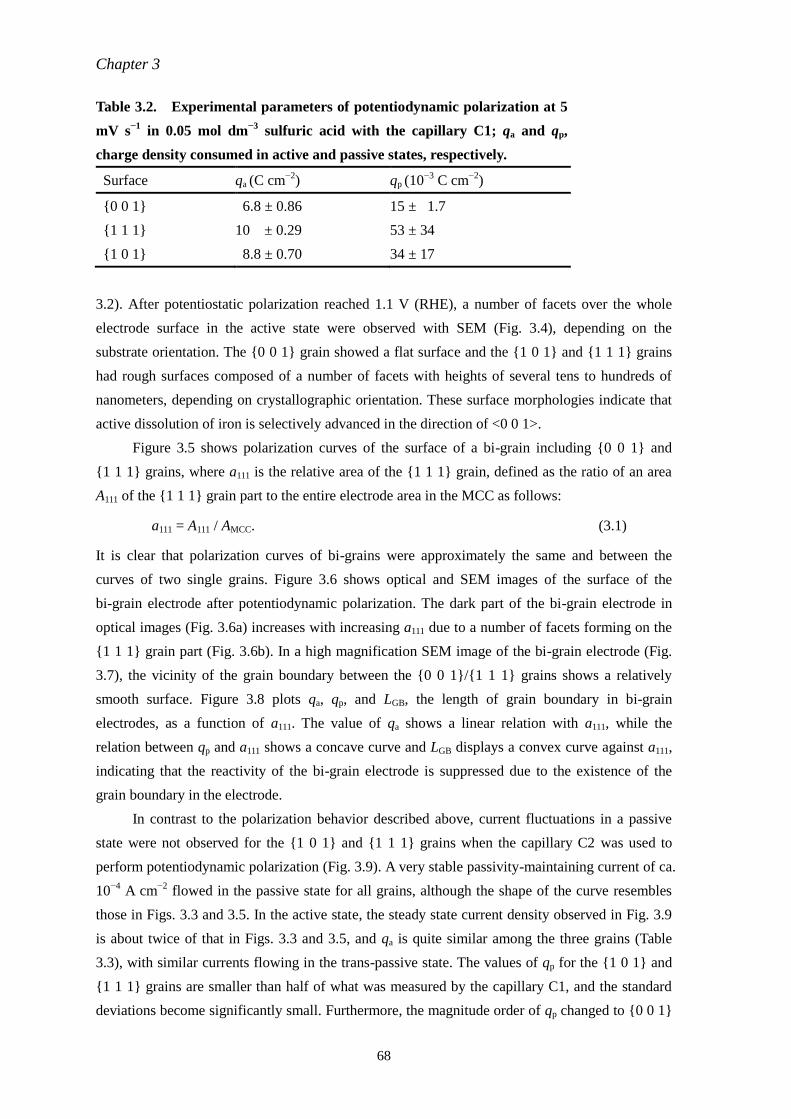
Chapter 3
68
Table 3.2. Experimental parameters of potentiodynamic polarization at 5
mV s−1
in 0.05 mol dm−3
sulfuric acid with the capillary C1; qa and qp,
charge density consumed in active and passive states, respectively.
Surface qa (C cm−2
) qp (10−3
C cm−2
)
{0 0 1} 6.8 ± 0.86 15 ± 1.7
{1 1 1} 10 ± 0.29 53 ± 34
{1 0 1} 8.8 ± 0.70 34 ± 17
3.2). After potentiostatic polarization reached 1.1 V (RHE), a number of facets over the whole
electrode surface in the active state were observed with SEM (Fig. 3.4), depending on the
substrate orientation. The {0 0 1} grain showed a flat surface and the {1 0 1} and {1 1 1} grains
had rough surfaces composed of a number of facets with heights of several tens to hundreds of
nanometers, depending on crystallographic orientation. These surface morphologies indicate that
active dissolution of iron is selectively advanced in the direction of <0 0 1>.
Figure 3.5 shows polarization curves of the surface of a bi-grain including {0 0 1} and
{1 1 1} grains, where a111 is the relative area of the {1 1 1} grain, defined as the ratio of an area
A111 of the {1 1 1} grain part to the entire electrode area in the MCC as follows:
a111 = A111 / AMCC. (3.1)
It is clear that polarization curves of bi-grains were approximately the same and between the
curves of two single grains. Figure 3.6 shows optical and SEM images of the surface of the
bi-grain electrode after potentiodynamic polarization. The dark part of the bi-grain electrode in
optical images (Fig. 3.6a) increases with increasing a111 due to a number of facets forming on the
{1 1 1} grain part (Fig. 3.6b). In a high magnification SEM image of the bi-grain electrode (Fig.
3.7), the vicinity of the grain boundary between the {0 0 1}/{1 1 1} grains shows a relatively
smooth surface. Figure 3.8 plots qa, qp, and LGB, the length of grain boundary in bi-grain
electrodes, as a function of a111. The value of qa shows a linear relation with a111, while the
relation between qp and a111 shows a concave curve and LGB displays a convex curve against a111,
indicating that the reactivity of the bi-grain electrode is suppressed due to the existence of the
grain boundary in the electrode.
In contrast to the polarization behavior described above, current fluctuations in a passive
state were not observed for the {1 0 1} and {1 1 1} grains when the capillary C2 was used to
perform potentiodynamic polarization (Fig. 3.9). A very stable passivity-maintaining current of ca.
10−4
A cm−2
flowed in the passive state for all grains, although the shape of the curve resembles
those in Figs. 3.3 and 3.5. In the active state, the steady state current density observed in Fig. 3.9
is about twice of that in Figs. 3.3 and 3.5, and qa is quite similar among the three grains (Table
3.3), with similar currents flowing in the trans-passive state. The values of qp for the {1 0 1} and
{1 1 1} grains are smaller than half of what was measured by the capillary C1, and the standard
deviations become significantly small. Furthermore, the magnitude order of qp changed to {0 0 1}
Chapter 3
69
Table 3.3. Experimental parameters of potentiodynamic polarization at 5
mV s−1
in 0.05 mol dm−3
sulfuric acid with the capillary C2; qa and qp,
charge density consumed in active and passive state, respectively.
Surface qa (C cm−2
) qp (10−3
C cm−2
)
{0 0 1} 17 ± 1.2 21 ± 2.1
{1 1 1} 17 ± 1.1 18 ± 1.3
{1 0 1} 17 ± 1.5 16 ± 1.4
> {1 1 1} > {1 0 1}. After potentiodynamic polarization using the capillary C1, the morphology of
the polarized sample surface became inhomogeneous (Figs. 3.10a and 3.10c). The middle part of
the sample surface showed a number of facets that appear as dark parts in an optical image;
however, the outside of the sample surface, which was laid under the silicone gasket during
polarization, showed no facets. On the contrary, after the polarization using the capillary C2, a
number of facets were formed over the entire electrode surface and the morphology of the surface
was homogeneous (Figs. 3.10b and 3.10d).
It is obvious that the transients of anodic currents depend on the geometry of the MCC.
Localized concentration of dissolved iron species at the solution/electrode interface induces
precipitation of iron oxides or iron hydroxides, and acidification of the solution simultaneously,
resulting in current oscillations in active to passive transition [9]. In this sense, it is considered
that the thick and wide silicone gasket rubber of the capillary C1 makes a tiny space between the
rubber and the sample surface in the MCC. Diffusion of ferrous ions generated at the sample
surface in an active state to bulk electrolyte is limited in the tiny space and the ions are highly
concentrated. This results in a decrease in local pH due to hydrolysis by the formation of iron
hydroxides, leading the destabilization of passivity. A smaller steady current in the active state
with the capillary C1 suggests that the diffusion of dissolved species is partially limited. The
current fluctuation observed in the passive state with the capillary C1 is probably related to a
roughness of the specimen surface under the silicone gasket. The concentration gradient of ferrous
ions on a rough surface destabilizes passivity rather than that on a smooth surface. Thus, it is also
thought that a relatively smooth surface in the vicinity of a grain boundary stabilizes the passivity
of the bi-grain electrode. In any cases, corrosion behavior in both active and passive states on
bi-grain electrodes seems to be explained by that on single grains. These results indicate that the
geometry of an MCC greatly affects electrochemical behavior of local surfaces.
During polarization in acidic media, the surface condition of an electrode is altered
chemically and electrochemically. The electrochemical behavior of the electrode surface
significantly suffers from the previous polarization under the condition of potentiodynamic
polarization. In this sense, the iron species generated in an active state affect the electrode
behavior in a passive state. The MCC is much more susceptible than macro-electrochemical cells
to dissolved species due to its small solution volume. Although there are some qualitative grain
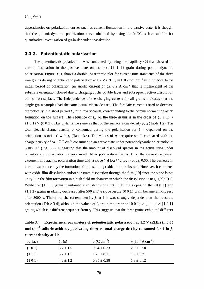
Chapter 3
70
dependencies on polarization curves such as current fluctuation in the passive state, it is thought
that the potentiodynamic polarization curve obtained by using the MCC is less suitable for
quantitative investigation of grain-dependent passivation.
3.3.2. Potentiostatic polarization
The potentiostatic polarization was conducted by using the capillary C3 that showed no
current fluctuation in the passive state on the iron {1 1 1} grain during potentiodynamic
polarization. Figure 3.11 shows a double logarithmic plot for current-time transients of the three
iron grains during potentiostatic polarization at 1.2 V (RHE) in 0.05 mol dm−3
sulfuric acid. In the
initial period of polarization, an anodic current of ca. 0.2 A cm−2
that is independent of the
substrate orientation flowed due to charging of the double layer and subsequent active dissolution
of the iron surface. The independence of the charging current for all grains indicates that the
single grain samples had the same actual electrode area. The faradaic current started to decrease
dramatically in a short period tpa of a few seconds, corresponding to the commencement of oxide
formation on the surface. The sequence of tpa on the three grains is in the order of {1 1 1} >
{1 0 1} > {0 0 1}. This order is the same as that of the surface atom density ρsurf (Table 1.2). The
total electric charge density qt consumed during the polarization for 1 h depended on the
orientation associated with tp (Table 3.4). The values of qt are quite small compared with the
charge density of ca. 17 C cm−2
consumed in an active state under potentiodynamic polarization at
5 mV s−1
(Fig. 3.9), suggesting that the amount of dissolved species in the active state under
potentiostatic polarization is very small. After polarization for ca. 10 s, the current decreased
exponentially against polarization time with a slope (–d log j / d log t) of ca. 0.65. The decrease in
current was caused by the formation of an insulating oxide on the substrate. However, it competes
with oxide film dissolution and/or substrate dissolution through the film [10] since the slope is not
unity like the film formation in a high field mechanism in which the dissolution is negligible [11].
While the {1 0 1} grain maintained a constant slope until 1 h, the slopes on the {0 0 1} and
{1 1 1} grains gradually decreased after 500 s. The slope on the {0 0 1} grain became almost zero
after 3000 s. Therefore, the current density jf at 1 h was strongly dependent on the substrate
orientation (Table 3.4), although the values of jf are in the order of {0 0 1} > {1 1 1} > {1 0 1}
grains, which is a different sequence from tp. This suggests that the three grains exhibited different
Table 3.4. Experimental parameters of potentiostatic polarization at 1.2 V (RHE) in 0.05
mol dm−3
sulfuric acid; tpa, passivating time; qt, total charge density consumed for 1 h; jf,
current density at 1 h.
Surface tpa (s) qt (C cm−2
) jf (10−6
A cm−2
)
{0 0 1} 3.7 ± 1.5 0.54 ± 0.33 2.9 ± 0.50
{1 1 1} 5.2 ± 1.1 1.2 ± 0.11 1.9 ± 0.21
{1 0 1} 4.6 ± 1.2 0.85 ± 0.38 1.3 ± 0.12
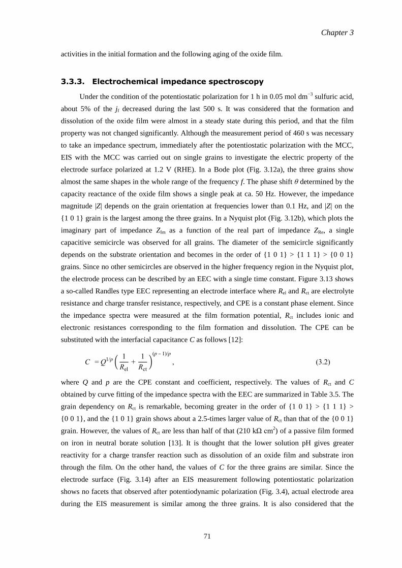
Chapter 3
71
activities in the initial formation and the following aging of the oxide film.
3.3.3. Electrochemical impedance spectroscopy
Under the condition of the potentiostatic polarization for 1 h in 0.05 mol dm−3
sulfuric acid,
about 5% of the jf decreased during the last 500 s. It was considered that the formation and
dissolution of the oxide film were almost in a steady state during this period, and that the film
property was not changed significantly. Although the measurement period of 460 s was necessary
to take an impedance spectrum, immediately after the potentiostatic polarization with the MCC,
EIS with the MCC was carried out on single grains to investigate the electric property of the
electrode surface polarized at 1.2 V (RHE). In a Bode plot (Fig. 3.12a), the three grains show
almost the same shapes in the whole range of the frequency f. The phase shift θ determined by the
capacity reactance of the oxide film shows a single peak at ca. 50 Hz. However, the impedance
magnitude |Z| depends on the grain orientation at frequencies lower than 0.1 Hz, and |Z| on the
{1 0 1} grain is the largest among the three grains. In a Nyquist plot (Fig. 3.12b), which plots the
imaginary part of impedance ZIm as a function of the real part of impedance ZRe, a single
capacitive semicircle was observed for all grains. The diameter of the semicircle significantly
depends on the substrate orientation and becomes in the order of {1 0 1} > {1 1 1} > {0 0 1}
grains. Since no other semicircles are observed in the higher frequency region in the Nyquist plot,
the electrode process can be described by an EEC with a single time constant. Figure 3.13 shows
a so-called Randles type EEC representing an electrode interface where Rel and Rct are electrolyte
resistance and charge transfer resistance, respectively, and CPE is a constant phase element. Since
the impedance spectra were measured at the film formation potential, Rct includes ionic and
electronic resistances corresponding to the film formation and dissolution. The CPE can be
substituted with the interfacial capacitance C as follows [12]:
C = Q1/p ( 1
Rel
+ 1
Rct
)(p – 1)/p
, (3.2)
where Q and p are the CPE constant and coefficient, respectively. The values of Rct and C
obtained by curve fitting of the impedance spectra with the EEC are summarized in Table 3.5. The
grain dependency on Rct is remarkable, becoming greater in the order of {1 0 1} > {1 1 1} >
{0 0 1}, and the {1 0 1} grain shows about a 2.5-times larger value of Rct than that of the {0 0 1}
grain. However, the values of Rct are less than half of that (210 kΩ cm2) of a passive film formed
on iron in neutral borate solution [13]. It is thought that the lower solution pH gives greater
reactivity for a charge transfer reaction such as dissolution of an oxide film and substrate iron
through the film. On the other hand, the values of C for the three grains are similar. Since the
electrode surface (Fig. 3.14) after an EIS measurement following potentiostatic polarization
shows no facets that observed after potentiodynamic polarization (Fig. 3.4), actual electrode area
during the EIS measurement is similar among the three grains. It is also considered that the
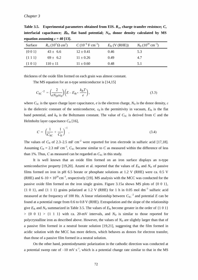
Chapter 3
72
Table 3.5. Experimental parameters obtained from EIS. Rct, charge transfer resistnce; C,
interfacial capacitance; Efb, flat band potential; ND, donor density calculated by MS
equation assuming ε = 40 [13].
Surface Rct (103 Ω cm
2) C (10
−6 F cm
−2) Efb (V (RHE)) ND (10
20 cm
−3)
{0 0 1} 43 ± 6.6 12 ± 0.41 0.46 5.3
{1 1 1} 69 ± 6.2 11 ± 0.26 0.49 4.7
{1 0 1} 110 ± 11 11 ± 0.60 0.48 5.1
thickness of the oxide film formed on each grain was almost constant.
The MS equation for an n-type semiconductor is [14,15]
CSC–2 = (
2
eNDεε0
) (E – Efb– kBT
e) , (3.3)
where CSC is the space charge layer capacitance, e is the electron charge, ND is the donor density, ε
is the dielectric constant of the semiconductor, ε0 is the permittivity in vacuum, Efb is the flat
band potential, and kB is the Boltzmann constant. The value of CSC is derived from C and the
Helmholtz layer capacitance CH [16],
C = (1
CSC
+ 1
CH )
–1
. (3.4)
The values of CH of 2.3–2.5 mF cm–2
were reported for iron electrode in sulfuric acid [17,18].
Assuming CH = 2.3 mF cm–2
, CSC became similar to C as measured within the difference of less
than 1%. Thus, C as measured can be regarded as CSC in this study.
It is well known that an oxide film formed on an iron surface displays an n-type
semiconductive property [19,20]. Azumi et al. reported that the values of Efb and ND of passive
films formed on iron in pH 6.5 borate or phosphate solutions at 1.2 V (RHE) were ca. 0.5 V
(RHE) and 6–10 × 1020
cm–3
, respectively [19]. MS analysis with the MCC was conducted for the
passive oxide film formed on the iron single grains. Figure 3.15a shows MS plots of {0 0 1},
{1 0 1}, and {1 1 1} grains polarized at 1.2 V (RHE) for 1 h in 0.05 mol dm–3
sulfuric acid
measured at the frequency of 100 Hz. A linear relationship between CSC–2
and potential E can be
found at a potential range from 0.6 to 0.8 V (RHE). Extrapolation and the slope of the relationship
give Efb and ND summarized in Table 3.5. The values of Efb become greater in the order of {1 0 1}
> {0 0 1} > {1 1 1} with ca. 20-mV intervals, and ND is similar to those reported for
polycrystalline iron as described above. However, the values of ND are slightly larger than that of
a passive film formed in a neutral borate solution [19,21], suggesting that the film formed in
acidic solution with the MCC has more defects, which behaves as donors for electron transfer,
than those of a passive film formed in a neutral solution.
On the other hand, potentiodynamic polarization in the cathodic direction was conducted at
a potential sweep rate of –10 mV s–1
, which is a potential change rate similar to that in the MS
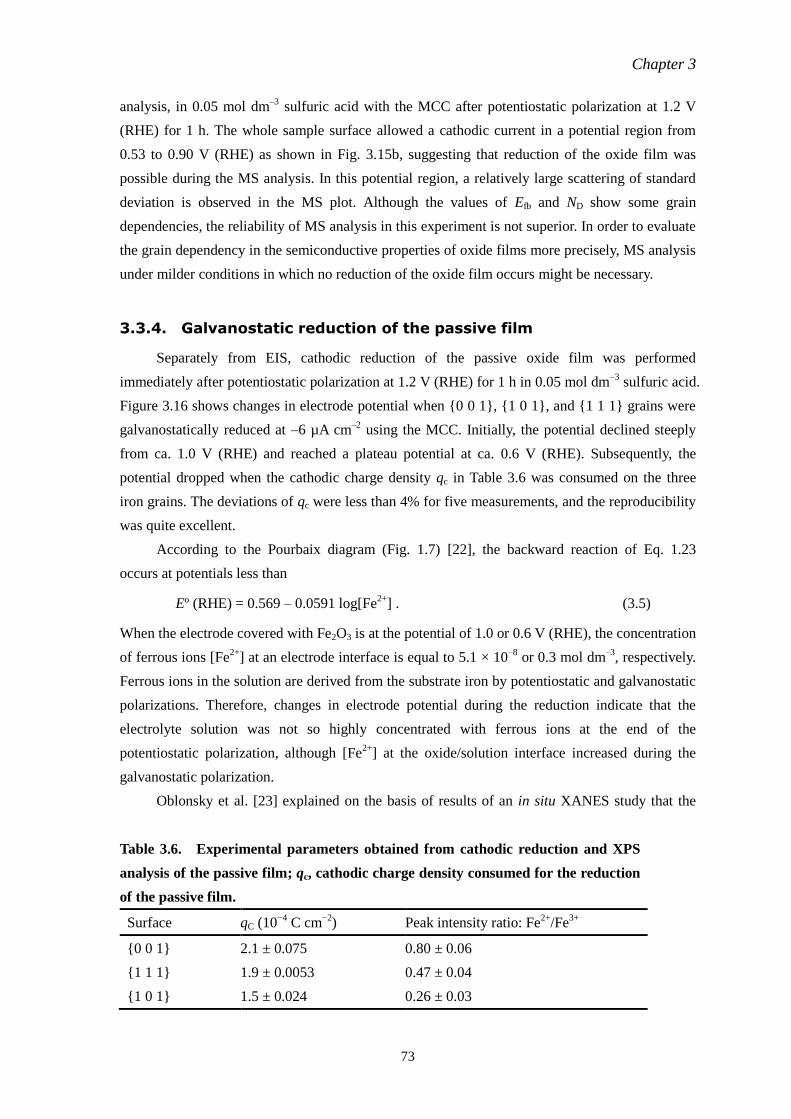
Chapter 3
73
analysis, in 0.05 mol dm–3
sulfuric acid with the MCC after potentiostatic polarization at 1.2 V
(RHE) for 1 h. The whole sample surface allowed a cathodic current in a potential region from
0.53 to 0.90 V (RHE) as shown in Fig. 3.15b, suggesting that reduction of the oxide film was
possible during the MS analysis. In this potential region, a relatively large scattering of standard
deviation is observed in the MS plot. Although the values of Efb and ND show some grain
dependencies, the reliability of MS analysis in this experiment is not superior. In order to evaluate
the grain dependency in the semiconductive properties of oxide films more precisely, MS analysis
under milder conditions in which no reduction of the oxide film occurs might be necessary.
3.3.4. Galvanostatic reduction of the passive film
Separately from EIS, cathodic reduction of the passive oxide film was performed
immediately after potentiostatic polarization at 1.2 V (RHE) for 1 h in 0.05 mol dm–3
sulfuric acid.
Figure 3.16 shows changes in electrode potential when {0 0 1}, {1 0 1}, and {1 1 1} grains were
galvanostatically reduced at –6 µA cm–2
using the MCC. Initially, the potential declined steeply
from ca. 1.0 V (RHE) and reached a plateau potential at ca. 0.6 V (RHE). Subsequently, the
potential dropped when the cathodic charge density qc in Table 3.6 was consumed on the three
iron grains. The deviations of qc were less than 4% for five measurements, and the reproducibility
was quite excellent.
According to the Pourbaix diagram (Fig. 1.7) [22], the backward reaction of Eq. 1.23
occurs at potentials less than
Eº (RHE) = 0.569 – 0.0591 log[Fe2+
] . (3.5)
When the electrode covered with Fe2O3 is at the potential of 1.0 or 0.6 V (RHE), the concentration
of ferrous ions [Fe2+
] at an electrode interface is equal to 5.1 × 10⁻⁸
or 0.3 mol dm–3
, respectively.
Ferrous ions in the solution are derived from the substrate iron by potentiostatic and galvanostatic
polarizations. Therefore, changes in electrode potential during the reduction indicate that the
electrolyte solution was not so highly concentrated with ferrous ions at the end of the
potentiostatic polarization, although [Fe2+
] at the oxide/solution interface increased during the
galvanostatic polarization.
Oblonsky et al. [23] explained on the basis of results of an in situ XANES study that the
Table 3.6. Experimental parameters obtained from cathodic reduction and XPS
analysis of the passive film; qc, cathodic charge density consumed for the reduction
of the passive film.
Surface qC (10−4
C cm−2
) Peak intensity ratio: Fe2+
/Fe3+
{0 0 1} 2.1 ± 0.075 0.80 ± 0.06
{1 1 1} 1.9 ± 0.0053 0.47 ± 0.04
{1 0 1} 1.5 ± 0.024 0.26 ± 0.03
Chapter 3
74
plateau potential under galvanostatic reduction of the passive film formed on iron in acetate buffer
represented the simultaneous reduction of Fe2O3 to Fe3O4 and Fe2+
as follows:
2Fe2O3 + 4H+ + 2e
– → Fe3O4 + Fe
2+ + 2H2O. (3.6)
Fe3O4 dissolves chemically in an acidic solution [22]. When the substrate iron is partially exposed
to the solution, the remaining oxide (including Fe2O3 and Fe3O4) seems to be removed rapidly
since an electrochemical dissolution of the substrate Fe can drive an electrochemical reduction of
the oxide. As a result, the potential shifts immediately to another plateau where hydrogen
evolution reaction on the substrate iron is dominant.
It is thought that the order of qc corresponds to the grain dependency on the amount of
Fe2O3 in the film. From Eq. 3.6, a charge density of 0.29 mC cm–2
was required to reduce a Fe2O3
layer with a thickness of 1 nm that was contained in the oxide film formed in an acidic solution
[4]. However, the values of qc are less than that required to reduce all of the Fe2O3. This indicates
that a chemical dissolution of the oxide film proceeded in parallel with the electrochemical
reactions of Eqs. 1.23 and/or 3.6 in an acidic solution [23]. Although qc indicates that the relative
thickness of the Fe2O3 layer becomes in the order of {0 0 1} > {1 1 1} > {1 0 1} grains, the
chemical dissolution make it difficult to estimate quantitatively the amount of Fe2O3 in the film
from the cathodic polarization in this study.
3.3.5. X-ray photoelectron spectroscopy
After potentiostatic polarization of a single grain with the MCC that has a tip diameter of ca.
250 µm, XPS analysis of the polarized surface was conducted with a photoelectron detection
diameter of 200 µm. Figure 3.17 shows Fe 2p3/2 photoelectron spectra obtained from the surfaces
of iron {0 0 1}, {1 0 1}, and {1 1 1} grains polarized at 1.2 V (RHE) for 1 h in 0.05 mol dm–3
sulfuric acid. Although several deconvolution components for iron oxides have been reported for
analyzing photoelectron spectra of passive oxide films on iron [24–26], Fe2+
and Fe3+
ions were
focused on for oxidized iron species in order to identify the grain dependency on the oxidation
state of iron atoms in the passive film. The spectra after background subtraction were
deconvoluted into three curves that represent different oxidation states of iron species, Fe3+
, Fe2+
,
and Fe0, using the XPS peak energies for the standards reported by Keller and Strehblow [25]. A
relatively large peak of Fe0 observed in Fig. 3.17 probably indicate that the thickness of the
passive film is similar or smaller than the escape depth of photoelectrons since an in elastic mean
free path of Fe at Kα radiation [27] is ca. 2 nm. Therefore, the intensity of Fe0 should be excluded
to discuss the grain dependency of the oxide film. The ratio Fe2+
/Fe3+
of peak intensity in Table
3.6 clearly depends on the substrate orientation. This indicates that the film composition depends
on the substrate orientation and that the relative quantity of Fe2+
in the film was larger in the order
of {0 0 1} > {1 1 1} > {1 0 1} grains.
Chapter 3
75
3.4. Discussion
A bi-layered structure of the passive film, an inner Fe3O4 layer and an outer γ-Fe2O3 layer
[4], was reported by Nishimura et al., who conducted ellipsometry and galvanostatic polarization
in pH 1.85 phosphate solution. When the oxide film formed on iron in sulfuric acid has a bi-layer
structure, grain-dependent layer structures as shown in Fig. 3.18 can be assumed. While both
oxide films have similar thicknesses, since the interfacial capacitance C is independent of
substrate orientation, they show different ratios in the thickness of the inner Fe3O4 layer and the
outer γ-Fe2O3 layer. On the {0 0 1} grain (Fig. 3.18a), for which the largest qc was consumed
during galvanostatic polarization among the three grains, the outer γ-Fe2O3 layer accounted for a
larger proportion of the film than did that of the {1 0 1} grain (Fig. 3.18c). The film structure of
the iron {1 1 1} grain is considered such that the ratio of Fe3O4/γ-Fe2O3 represents a value
between those of the iron {0 0 1} and {1 0 1} grains (Fig. 3.18b). Since the electrical resistivity ρ
of Fe3O4 is significantly smaller than that of γ-Fe2O3 (ρ = 10−4
Ω m [28] and 105–10
7 Ω m [29–31]
for Fe3O4 and γ-Fe2O3 respectively.), most of the potential drop in the oxide film during
potentiostatic polarization exists in the γ-Fe2O3 layer, and Rct expresses the resistance to the
migration of ions driven by the potential drop. However, the magnitude order of Rct and qc showed
inverse correlation, even though thicker oxide typically shows higher electric or ionic resistances.
XPS analysis demonstrated that the Fe3+
/Fe2+
ratio in the oxide became greater in the same order
as that of Rct. Thus, the concentration of defects that trap Fe2+
ions as impurities and provide the
ionic conduction pass of the oxide becomes larger in the order of {0 0 1} > {1 1 1} > {1 0 1}.
Generation of Fe3O4, which introduces Fe2+
ions into the oxide film, is thermodynamically
spontaneous in γ-Fe2O3. For example, at the metal/film interface, the following reaction
progresses, since the Gibbs energy ∆G is equal to –133.0 kJ mol−1
:
Fe + 4γ-Fe2O3 → 3Fe3O4, (3.7)
where the ∆G of the formation of Fe3O4 and γ-Fe2O3 are –1014.88 kJ mol–1
and –727.9 kJ mol–1
respectively [28,32]. Here, the surface energy γ of a bcc lattice structure is greater in the order of
{0 0 1} > {1 1 1} > {1 0 1} grains (Table 1.2). It is reasonable that the {1 0 1} grain of bcc iron
has a low activity for Eq. 3.7 and is more impoverished in Fe2+
than the other grains.
Greater ionic defects in the oxide film allow a larger ionic current, and oxide ions [33]
and/or alternative cations [34] carry the ionic current in the anodic oxide film on iron. Davenport
et al. conducted in situ surface XRD and suggested that the passive film formed on the iron
(0 0 1) face was less defective than that formed on the iron (1 0 1) face due to the larger grain size
and fewer antiphase boundaries of the oxide film on the (1 0 1) face [35]. Their results measured
in pH 8.4 borate solution indicate that the {0 0 1} grain shows a higher ionic resistance than that
of the {1 0 1} grain. However, the {1 0 1} grain exhibited the largest Rct. This inconsistency can
be caused by the difference of the acidity of electrolyte solution. Under potentiostatic anodic
polarization in a passive state, the dissolution of an oxide film and/or substrate iron through the
Chapter 3
76
oxide film occurs in acidic solution, whereas it is negligible in neutral solution. Thus, it is
considered that the passive oxide film formed in pH 1.3 sulfuric acid has different defect
concentration due to the dissolution compared with that formed in neutral solution. The defect
concentration is the largest for the oxide film formed on the {0 0 1} grain and is the smallest for
that on the {1 0 1} grain. As a result, the migration rate of ions thorough the defect and the
dissolution rate of the oxide and substrate become greater in the order of {0 0 1} > {1 1 1} >
{1 0 1} grains, that is the inverse order of Rct. The dominant defects in the oxide film are
considered to be oxygen vacancies and/or iron interstitials [36], and grain boundaries between
grains of the oxide. It is thought that the grain-dependent defect structure is caused by different γ
and epitaxial relation between the substrate and oxide.
3.5. Conclusions
Grain-dependent passivation of iron single grains in sulfuric acid was investigated
individually with an MCC. Under the condition of potentiostatic polarization, iron {0 0 1},
{1 0 1}, and {1 1 1} grains showed different passivation behavior, and the current density after
polarization for 1 h became larger in the order of {0 0 1} > {1 1 1} > {1 0 1}. EIS following the
passivation revealed that the charge transfer resistance of the passive film formed on the iron
single grains greatly depended on the substrate orientation and exhibited a larger value in the
order of {1 0 1} > {1 1 1} > {0 0 1}. It was considered from galvanostatic reduction and XPS
analysis that the structure of the passive film formed on iron depended on the substrate orientation
due to the different surface energy of bcc iron. Considering that the structure of the oxide film
formed in sulfuric acid was bi-layered with an inner Fe3O4 layer and an outer γ-Fe2O3 layer, the
ratio of these two oxide layers depended on the substrate orientation. However, the thickness of a
highly-resistive γ-Fe2O3 layer and the charge transfer resistance inversely correlated. It was
considered that the defect concentration depends on the substrate orientation due to different
surface energy and/or epitaxial relation between the substrate and oxide.
References
[1] N. Sato, in Passivity of metals, R. P. Frankental and J. Kruger, Editors, p. 29, The
Electrochemical Society Inc., Princeton, NJ (1978).
[2] N. Sato and G. Okamoto, in Comprehensive Treatise of Electrochemistry Vol. 4:
Electrochemical Materials Science, J. O. M. Bockris, B. E. Conway, E. Yeager, and R. E.
White, Editors, p. 193, Plenum Press, New York and London (1981).
[3] K. Fushimi and M. Seo, Electrochim. Acta, 47, 121 (2001).
[4] R. Nishimura, K. Kudo, and N. Sato, Surf. Sci., 96, 413 (1980).
Chapter 3
77
[5] T. J. Chuang, C. R. Brundle, and K. Wandelt, Thin Solid Films, 53, 19 (1978).
[6] E. Desimoni, G. I. Casella, A. M. Salvi, T. R. I. Cataldi, and A. Morone, Carbon, 30, 527
(1992).
[7] D. A. Shirley, Phys. Rev. B, 5, 4709 (1972).
[8] K. Fushimi, K. Miyamoto, and H. Konno, Electrochim. Acta, 55, 7322 (2010).
[9] B. Rush and J. Newman, J. Electrochem. Soc., 142, 3770 (1995).
[10] K. J. Vetter and F. Gorn, Electrochim. Acta, 18, 321 (1973).
[11] G. T. Burstein and A. J. Davenport, J. Electrochem. Soc., 136, 936 (1989).
[12] G. J. Brug, A. L. G. van den Eeden, M. Sluyters-Rehbach, and J. H. Sluyters, J. Electroanal.
Chem. Interfacial Electrochem., 176, 275 (1984).
[13] K. Azumi, T. Ohtsuka, and N. Sato, Trans. Jpn. Inst. Met., 27, 382 (1986).
[14] N. F. Mott, Proc. R. Soc. London A, 171, 27 (1939).
[15] W. Schottky, Zeitschrift für Phys., 113, 367 (1939).
[16] J. W. Schultze and M. M. Lohrengel, Electrochim. Acta, 45, 2499 (2000).
[17] N. Krithivasan, T. Tsuru, and S. Haruyama, Boshoku Gijutsu, 29, 275 (1980).
[18] C. Jeyaprabha, S. Sathiyanarayanan, and G. Venkatachari, Appl. Surf. Sci., 246, 108 (2005).
[19] K. Azumi, T. Ohtsuka, and N. Sato, J. Electrochem. Soc., 134, 1352 (1987).
[20] J. Wielant, V. Goossens, R. Hausbrand, and H. Terryn, Electrochim. Acta, 52, 7617 (2007).
[21] T. Yamamoto, K. Fushimi, S. Miura, and H. Konno, J. Electrochem. Soc., 157, C231 (2010).
[22] M. Pourbaix, Atlas of Electrochemical Equilibria in Aqueous Solution, 2nd English ed.,
p. 307, National Association of Corrosion Engineers, Houston (1974).
[23] L. J. Oblonsky, M. P. Ryan, and H. S. Isaacs, Corros. Sci., 42, 229 (2000).
[24] K. Asami and K. Hashimoto, Corros. Sci., 17, 559 (1977).
[25] P. Keller and H.-H. Strehblow, Corros. Sci., 46, 1939 (2004).
[26] R.-H. Jung, H. Tsuchiya, and S. Fujimoto, Corros. Sci., 58, 62 (2012).
[27] T. Nagatomi, S. Tanuma, and K. Goto, Surf. Interface Anal., 42, 1537 (2010).
[28] G. V. Samsonov, The Oxide Handbook, p. 272, IFI/Plenum, New York (1973).
[29] K. Iwauchi, Jpn. J. Appl. Phys., 10, 1520 (1971).
[30] K. S. Rane, A. K. Nikumbh, and A. J. Mukhedkar, J. Mater. Sci., 16, 2387 (1981).
[31] V. A. Hiremath and A. Venkataraman, Bull. Mater. Sci., 26, 391 (2003).
[32] J. Majzlan, K.-D. Grevel, and A. Navrotsky, Am. Mineral., 88, 855 (2003).
[33] N. Sato and T. Noda, Electrochim. Acta, 22, 839 (1977).
[34] S. C. Hendy, N. J. Laycock, and M. P. Ryan, J. Electrochem. Soc., 152, B271 (2005).
[35] A. J. Davenport, L. J. Oblonsky, M. P. Ryan, and M. F. Toney, J. Electrochem. Soc., 147,
2162 (2000).
[36] S. Ahn and H. Kwon, J. Electroanal. Chem., 579, 311 (2005).
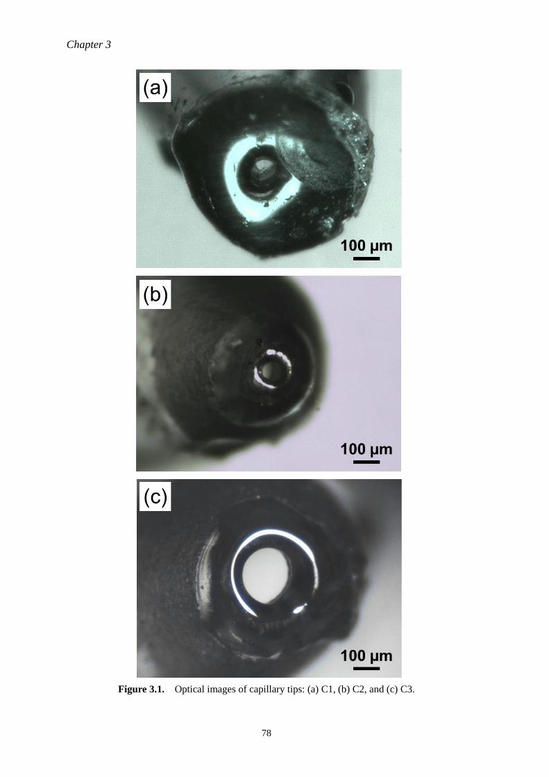
Chapter 3
78
Figure 3.1. Optical images of capillary tips: (a) C1, (b) C2, and (c) C3.
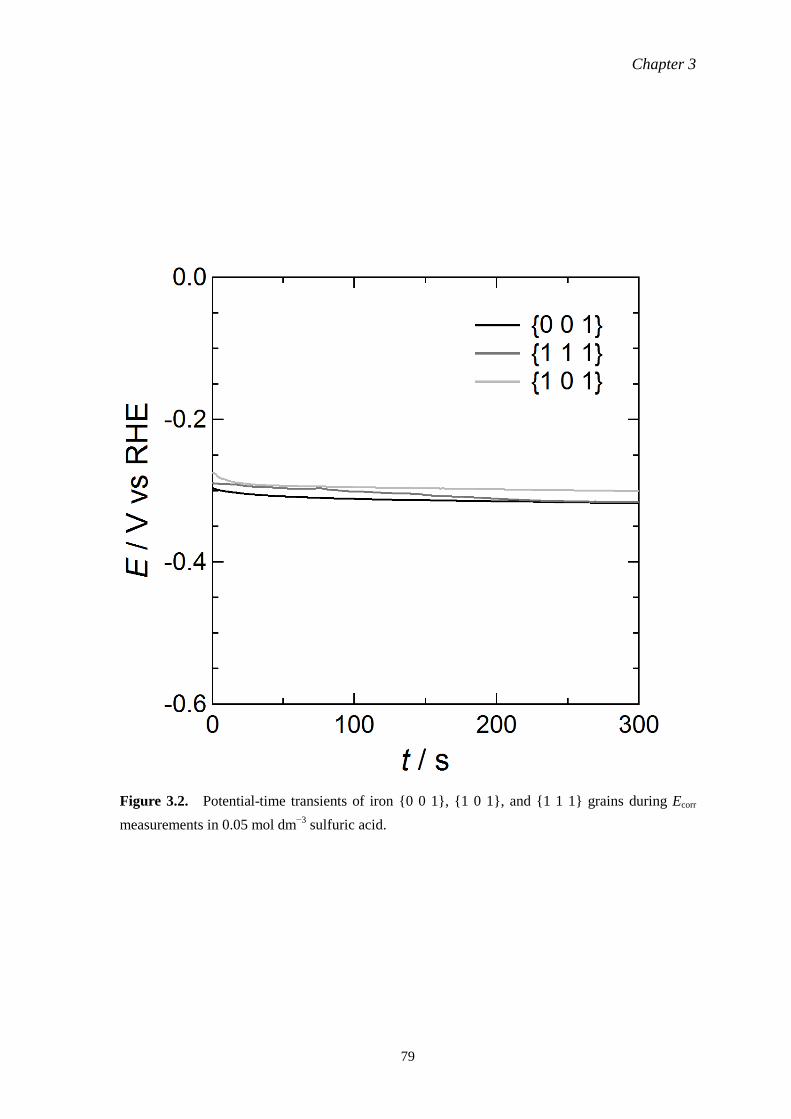
Chapter 3
79
Figure 3.2. Potential-time transients of iron {0 0 1}, {1 0 1}, and {1 1 1} grains during Ecorr
measurements in 0.05 mol dm−3
sulfuric acid.
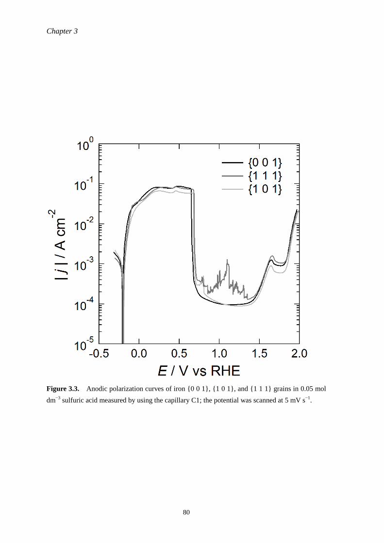
Chapter 3
80
Figure 3.3. Anodic polarization curves of iron {0 0 1}, {1 0 1}, and {1 1 1} grains in 0.05 mol
dm−3
sulfuric acid measured by using the capillary C1; the potential was scanned at 5 mV s−1
.
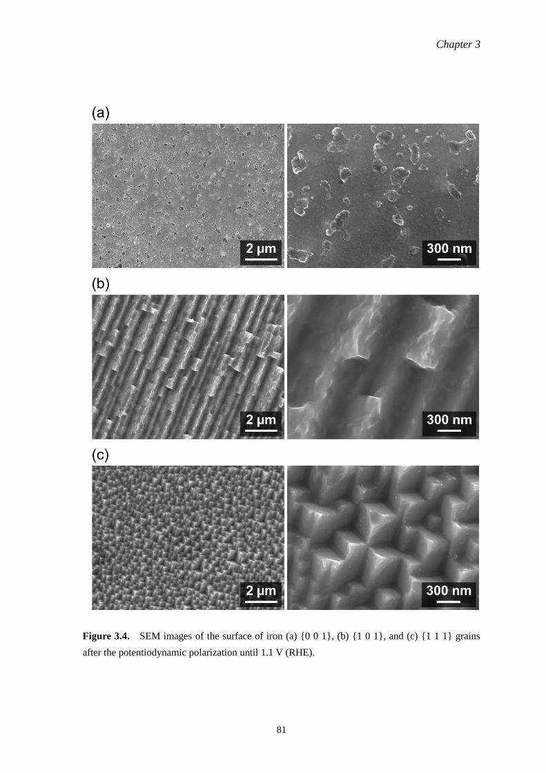
Chapter 3
81
Figure 3.4. SEM images of the surface of iron (a) {0 0 1}, (b) {1 0 1}, and (c) {1 1 1} grains
after the potentiodynamic polarization until 1.1 V (RHE).
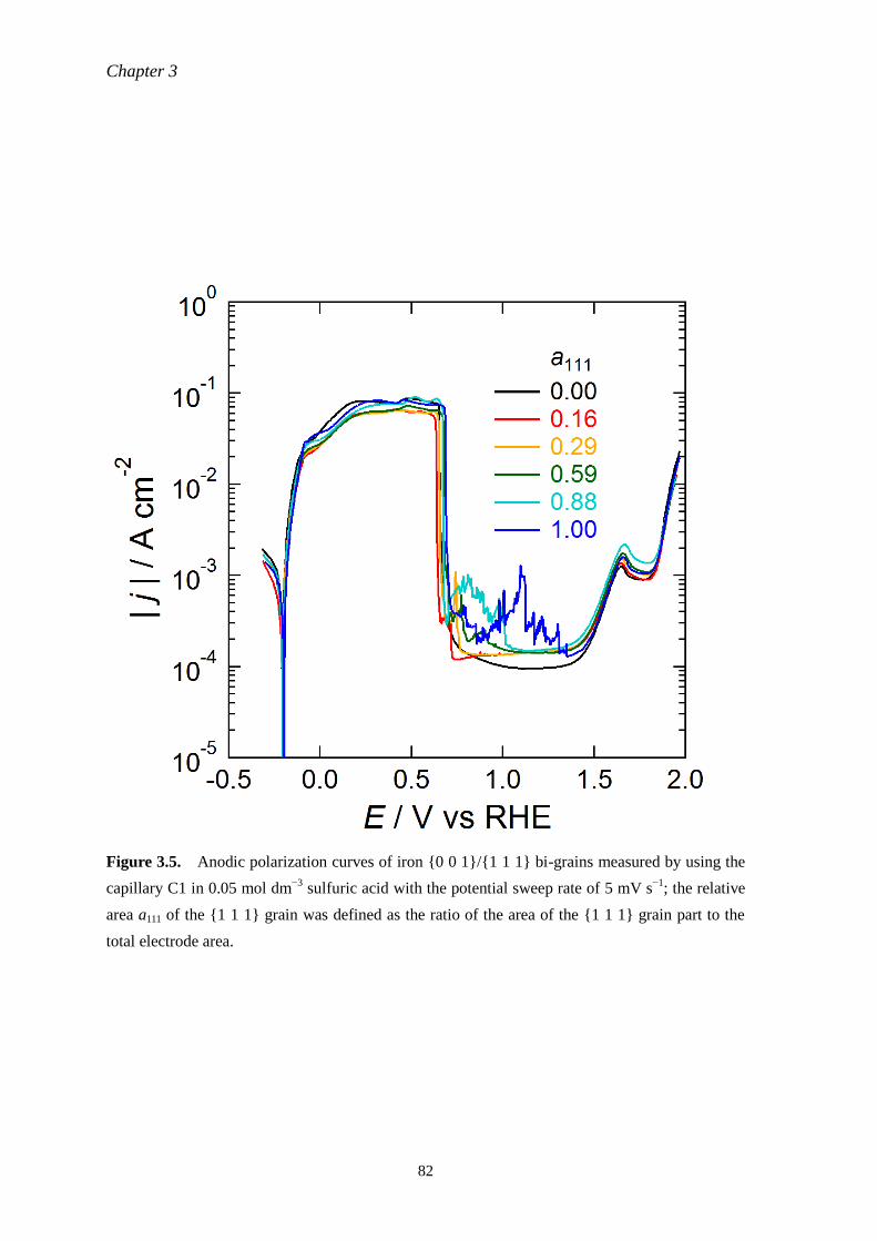
Chapter 3
82
Figure 3.5. Anodic polarization curves of iron {0 0 1}/{1 1 1} bi-grains measured by using the
capillary C1 in 0.05 mol dm−3
sulfuric acid with the potential sweep rate of 5 mV s−1
; the relative
area a111 of the {1 1 1} grain was defined as the ratio of the area of the {1 1 1} grain part to the
total electrode area.
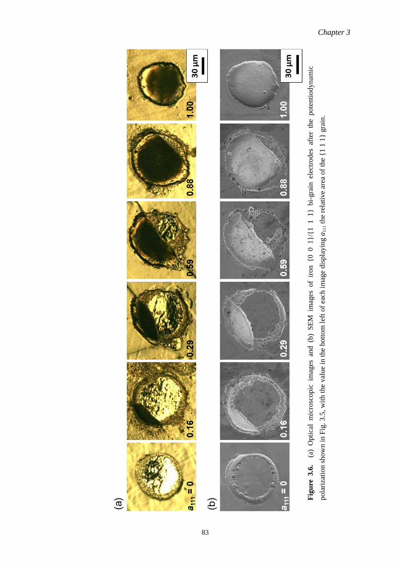
Chapter 3
83
Fig
ure
3
.6.
(a
) O
pti
cal
mic
rosc
opic
im
ages
an
d (b
) S
EM
im
ages
of
iron {0 0 1}/{
1
1 1
} b
i-gra
in el
ectr
od
es af
ter
the
po
ten
tio
dyn
amic
pola
riza
tio
n s
ho
wn
in
Fig
. 3
.5, w
ith
the
val
ue
in t
he
bott
om
lef
t of
each
im
age
dis
pla
yin
g a
111 t
he
rela
tive
area
of
the
{1
1 1
} g
rain
.
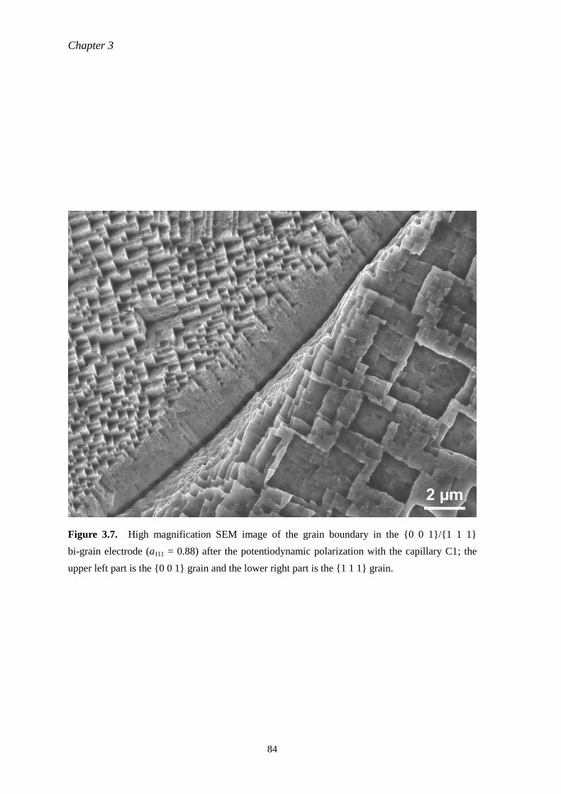
Chapter 3
84
Figure 3.7. High magnification SEM image of the grain boundary in the {0 0 1}/{1 1 1}
bi-grain electrode (a111 = 0.88) after the potentiodynamic polarization with the capillary C1; the
upper left part is the {0 0 1} grain and the lower right part is the {1 1 1} grain.
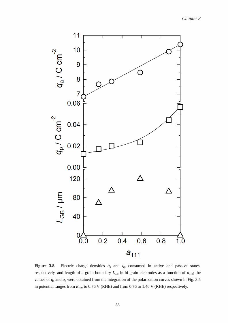
Chapter 3
85
Figure 3.8. Electric charge densities qa and qp consumed in active and passive states,
respectively, and length of a grain boundary LGB in bi-grain electrodes as a function of a111; the
values of qa and qp were obtained from the integration of the polarization curves shown in Fig. 3.5
in potential ranges from Ecorr to 0.76 V (RHE) and from 0.76 to 1.46 V (RHE) respectively.
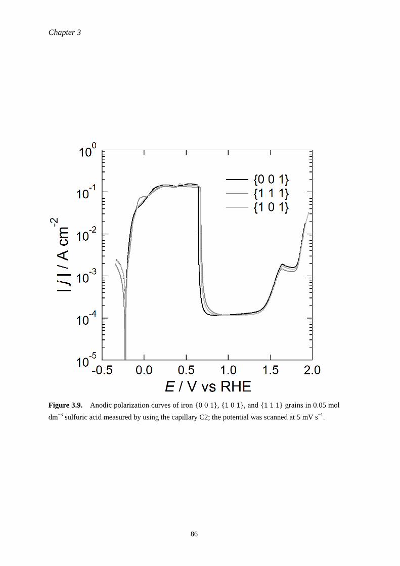
Chapter 3
86
Figure 3.9. Anodic polarization curves of iron {0 0 1}, {1 0 1}, and {1 1 1} grains in 0.05 mol
dm−3
sulfuric acid measured by using the capillary C2; the potential was scanned at 5 mV s−1
.
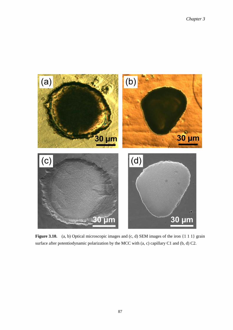
Chapter 3
87
Figure 3.10. (a, b) Optical microscopic images and (c, d) SEM images of the iron {1 1 1} grain
surface after potentiodynamic polarization by the MCC with (a, c) capillary C1 and (b, d) C2.
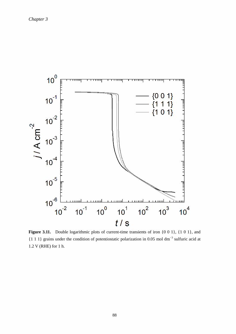
Chapter 3
88
Figure 3.11. Double logarithmic plots of current-time transients of iron {0 0 1}, {1 0 1}, and
{1 1 1} grains under the condition of potentiostatic polarization in 0.05 mol dm−3
sulfuric acid at
1.2 V (RHE) for 1 h.

Chapter 3
89
Figure 3.12. (a) Bode plot and (b) Nyquist plot of iron {0 0 1}, {1 0 1}, and {1 1 1} grains
polarized at 1.2 V (RHE) for 1 h in 0.05 mol dm−3
sulfuric acid.
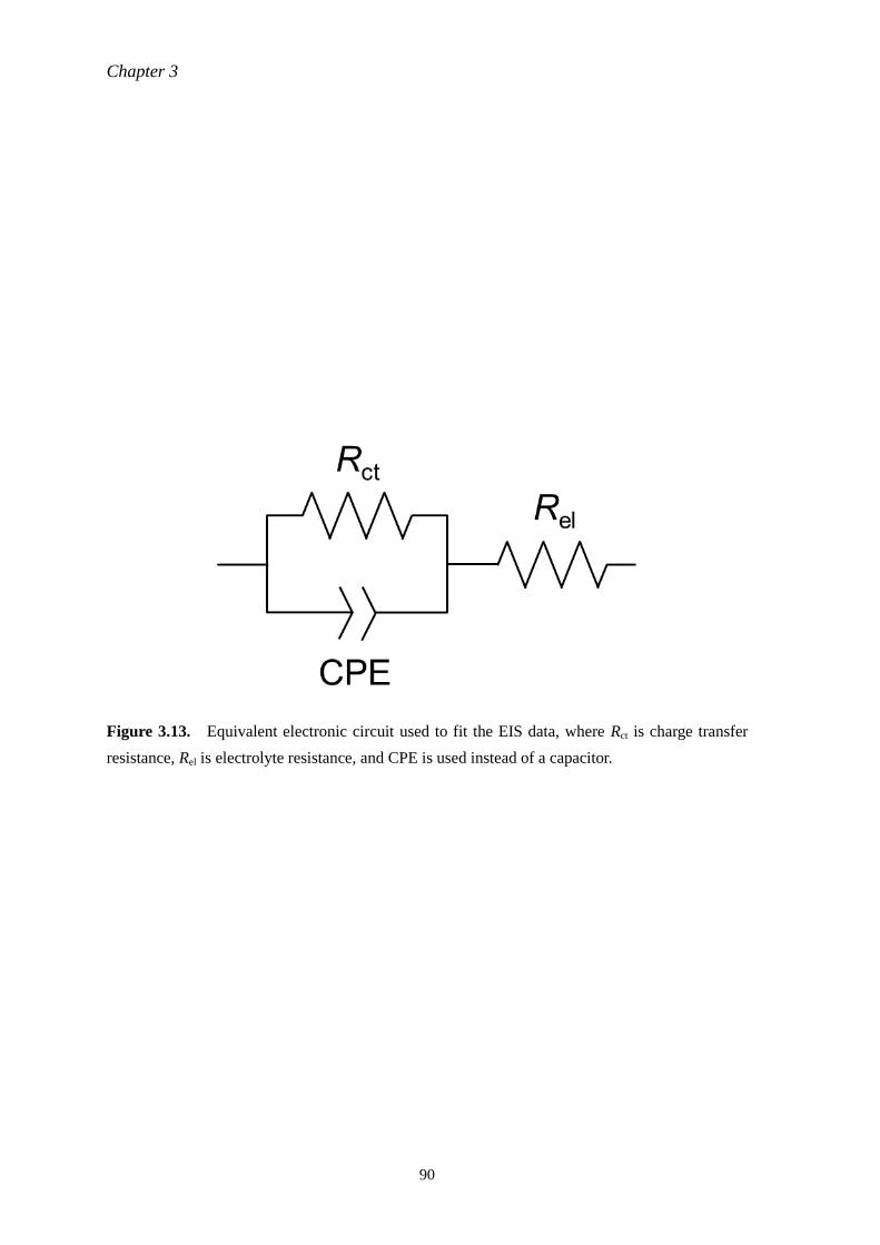
Chapter 3
90
Figure 3.13. Equivalent electronic circuit used to fit the EIS data, where Rct is charge transfer
resistance, Rel is electrolyte resistance, and CPE is used instead of a capacitor.
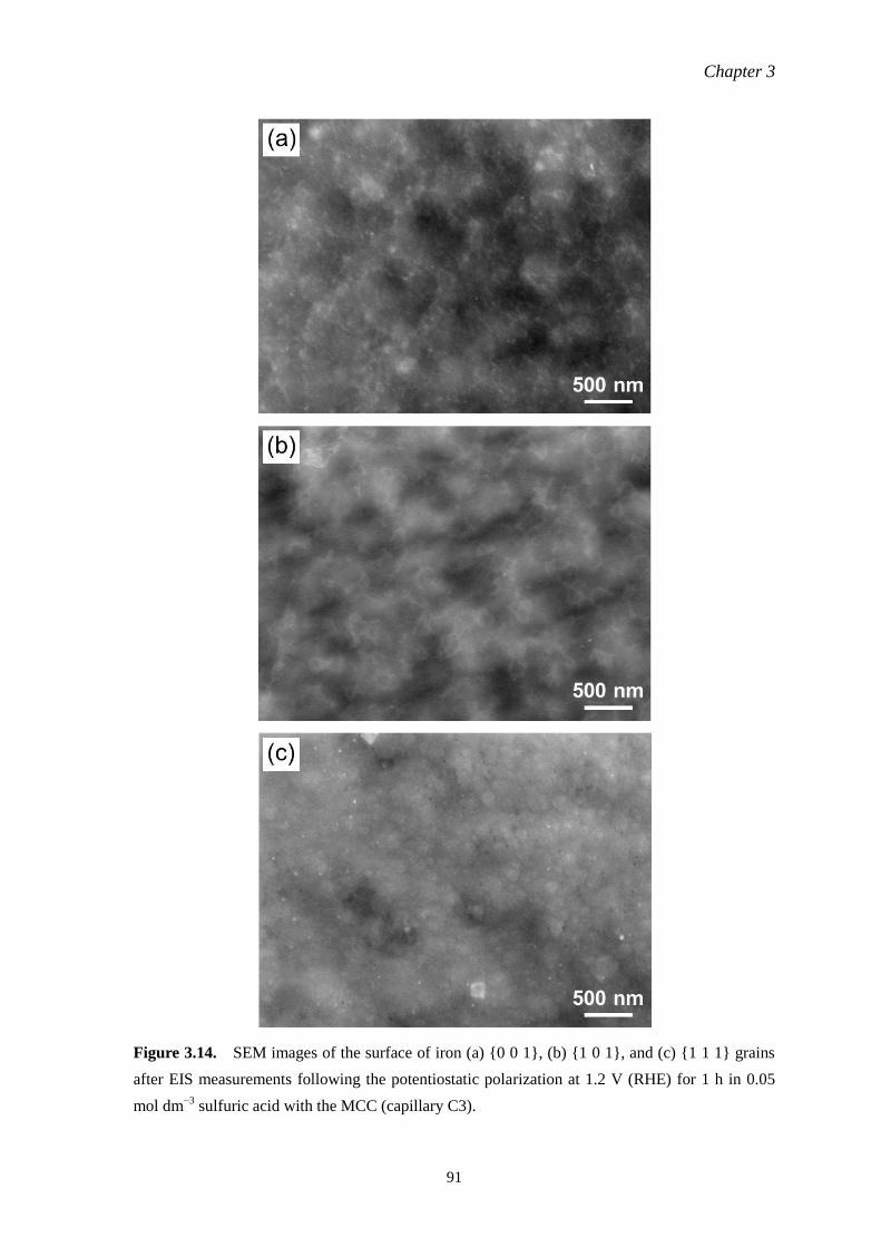
Chapter 3
91
Figure 3.14. SEM images of the surface of iron (a) {0 0 1}, (b) {1 0 1}, and (c) {1 1 1} grains
after EIS measurements following the potentiostatic polarization at 1.2 V (RHE) for 1 h in 0.05
mol dm−3
sulfuric acid with the MCC (capillary C3).
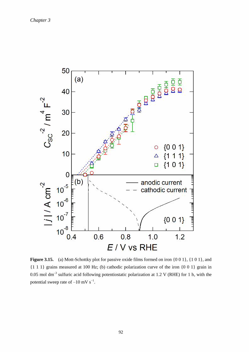
Chapter 3
92
Figure 3.15. (a) Mott-Schottky plot for passive oxide films formed on iron {0 0 1}, {1 0 1}, and
{1 1 1} grains measured at 100 Hz; (b) cathodic polarization curve of the iron {0 0 1} grain in
0.05 mol dm–3
sulfuric acid following potentiostatic polarization at 1.2 V (RHE) for 1 h, with the
potential sweep rate of –10 mV s−1
.
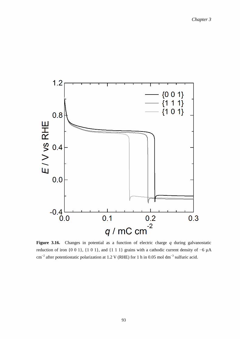
Chapter 3
93
Figure 3.16. Changes in potential as a function of electric charge q during galvanostatic
reduction of iron {0 0 1}, {1 0 1}, and {1 1 1} grains with a cathodic current density of −6 µA
cm−2
after potentiostatic polarization at 1.2 V (RHE) for 1 h in 0.05 mol dm−3
sulfuric acid.
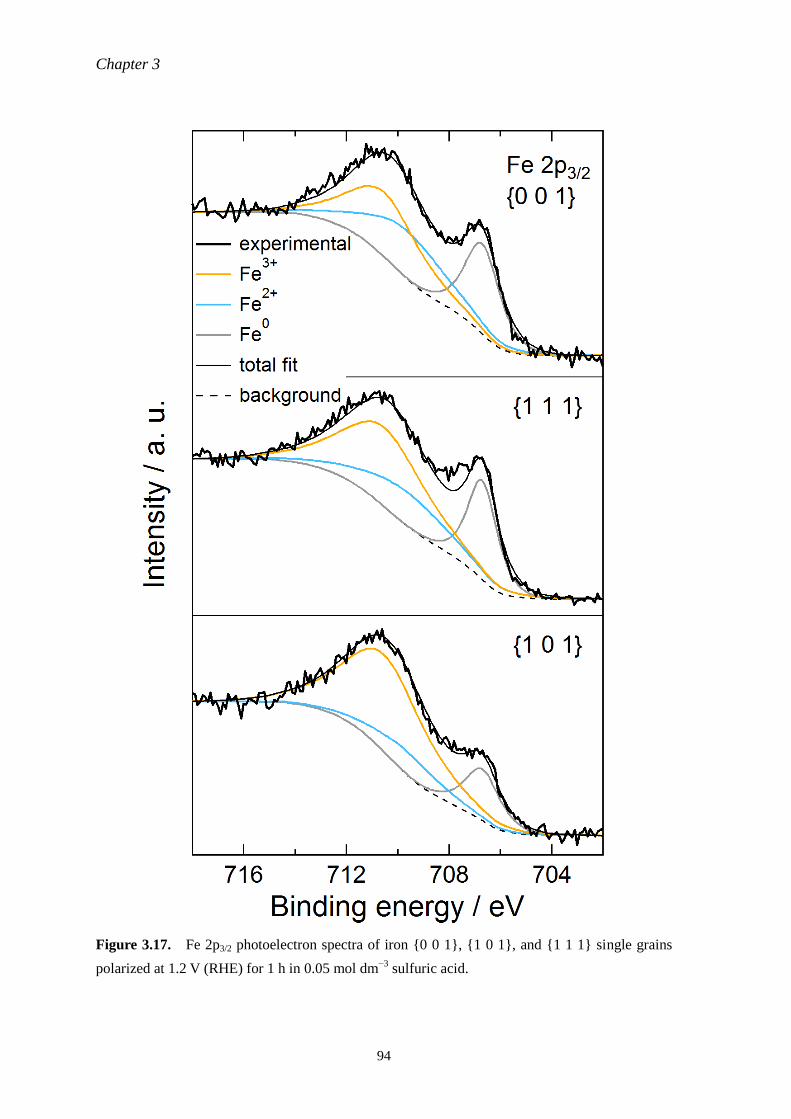
Chapter 3
94
Figure 3.17. Fe 2p3/2 photoelectron spectra of iron {0 0 1}, {1 0 1}, and {1 1 1} single grains
polarized at 1.2 V (RHE) for 1 h in 0.05 mol dm−3
sulfuric acid.
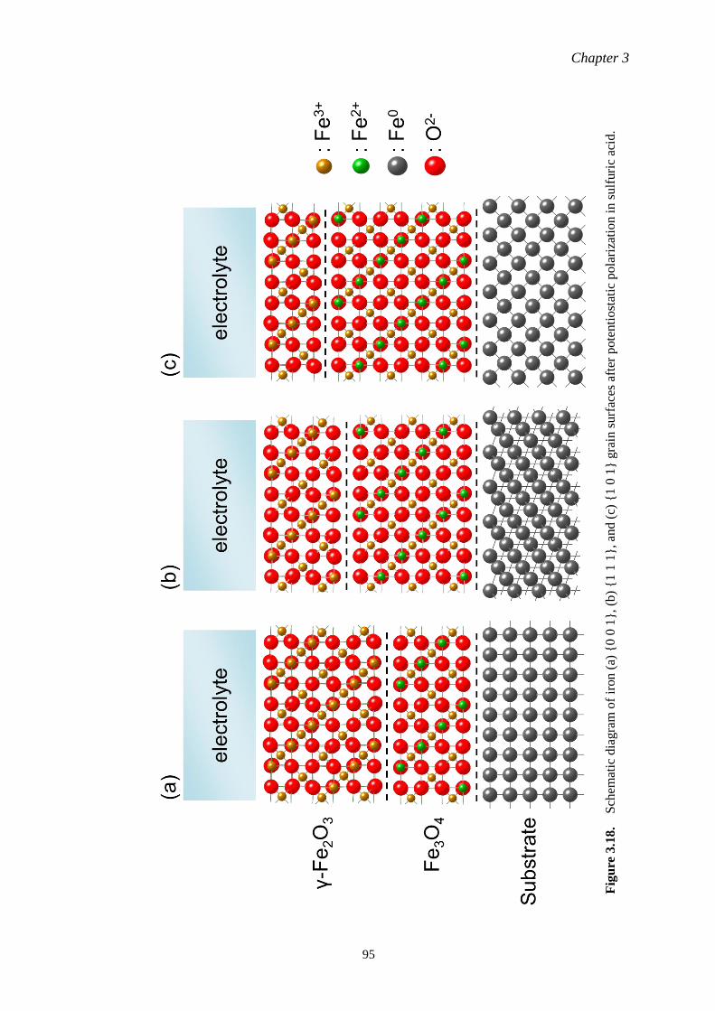
Chapter 3
95
Fig
ure
3.1
8.
S
chem
atic
dia
gra
m o
f ir
on (
a) {
0 0
1},
(b)
{1 1
1}, and (
c) {
1 0
1} g
rain
surf
aces
aft
er p
ote
nti
ost
atic
pola
riza
tio
n i
n s
ulf
uri
c ac
id.
Chapter 4
96
Chapter 4
Heterogeneity of thermally
grown oxide film observed by
two-dimensional ellipsometry
4.1. Introduction
A thermal oxide film grows on the surface of metals and alloys when it is exposed to a high
temperature atmosphere. Chemical characteristics of oxide such as corrosion resistance generally
differ from those of base metals. Thus, it is important to know the characteristics of the thermally
oxidized surface of metals and alloys to avoid undesired degradation of metallic materials. It has
been shown that thermally grown oxides formed on pure iron have characteristic composition,
structure, and thickness depending on oxidation conditions such as temperature, oxygen partial
pressure, and the presence of water vapor [1–3]. The crystallographic orientation of the iron
surface is also one of the factors that influence the rate of formation of thermal oxides.
Orientation-dependent formation of an oxide on an iron single crystal has been reported [4–6]. It
has been shown that the surface orientation greatly affects oxide formation at temperatures of 473
to 623 K、a temperature range at which recrystallization of iron is very slow and FeO does not
form due to its thermodynamic instability [7]. Orientation dependence on oxide thickness was
observed during an oxidation period of less than 1 h. Steels are generally used as polycrystalline
substances with surfaces consisting of numerous grains with different orientations and it is
apparent that the characteristics of a thermally oxidized polycrystalline iron surface are
heterogeneous. Pryor and Evans observed non-uniform dissolution of thermally grown oxide on
iron in dilute hydrochloric acid due to the heterogeneity of oxide thickness [8]. When the oxide
locally degrades and the substrate is partially exposed to a corrosive environment, localized
corrosion can occur. However, the heterogeneity of the oxidized surface was overlooked when
researchers investigated the characteristics and growth behavior of thermal oxides formed on iron.
For example, the thickness of an oxide layer on polycrystalline iron was usually reported as an
average value of the whole surface [9]; the distribution of oxide thicknesses that depended on the
each grain of a polycrystalline iron surface was not considered. The requirement to average
characteristics of a surface oxide was partly due to the lack of a measurement technique to
investigate both the numerous crystallographic orientations on a polycrystalline surface and the
characteristics of all of the oxides formed on each grain of the polycrystalline surface. Recently,
Chapter 4
97
EBSD patterning has been used for the identification of surface crystallographic orientations of
polycrystalline metals as applied to iron in 2.1.3. Precise crystal structures of relatively thick
thermal oxides, so-called “oxide scales”, formed on low-carbon steel [10] and pure iron [11] were
also determined by EBSD. However, despite the development of high-precision measurement
techniques, there has still been no report on the heterogeneous thermally oxidized surface of
polycrystalline iron.
In Chapter 3, the MCC fabricated in Chapter 2 successfully demonstrated the
grain-dependent electric properties of passive films formed on iron in sulfuric acid. In this chapter,
the heterogeneity of a thermally oxidized polycrystalline iron surface was visualized using 2D
ellipsometry, with the characteristics of the oxidized surface of each grain investigated by the
MCC method. Furthermore, grain-dependent degradation of the oxidized surface was observed by
means of in situ 2D ellipsometry and orientation-dependent growth of the thermal oxide film was
discussed.
4.2. Experimental
4.2.1. Sample preparation
After mirror-like polishing and EBSD patterning as described in section 2.1, the sample was
oxidized in a muffle furnace (KDF-S70, Denken-Highdental) at 573 K in air for 1 h. This
temperature is suitable for both MCC measurements and ellipsometry, since thick oxide films
formed at temperatures above 573 K showed too much electronic resistance and impedance
measurement became difficult, while thin oxide films formed below 573 K showed less grain
dependency. Finally, the sample was cooled to ambient temperature in open air.
4.2.2. Characterization of the oxidized surface
The oxidized surface of each grain was characterized by using a confocal Raman
microscope (XploRA, HORIBA) with a probe area of ca. 1 µm in diameter. A diode laser with a
wavelength of 532 nm was used for the excitation of Raman scattering. The power of the incident
laser was confined to 2 mW by filtering to avoid any change in the composition of the sample
surface, and a single Raman spectrum was scanned 64 times. In fact, no visual change was
observed on the sample surface after a Raman spectroscopic measurement for 280 s.
The oxidized surface was also characterized with XPS. The JPS-9200 photoelectron
spectrometer with Al Kα radiation operating at 100 W (10 kV, 10 mA) collected photoelectrons
emitted from the oxidized polycrystalline substrate and α-Fe2O3 powder (purity: 99.9%, Wako
Pure Chem. Ind., Ltd.) on a conductive carbon tape as a reference.
The morphology of the oxidized surface was observed with the JSM-6500F field-emission
Chapter 4
98
SEM and secondary electron (SE) images were collected. Furthermore, in order to observe the
cross-sectional structure of the oxidized sample surface, the sample was prepared by a cross
section polisher (CP) (SM-09010, JEOL) as follows. The sample specimen mounted in acrylic
resin was ground parallel to the sample ND with #800 SiC paper, and a sample cross section was
fabricated by using an Ar ion beam with an acceleration voltage of 6 kV. The cross section of the
sample was observed with a field-emission SEM (JSM-7001FA, JEOL). Backscattered electron
(BE) images were collected to observe the compositional distribution in the oxidized surface.
4.2.3. Two-dimensional ellipsometry
The thickness distribution of an oxidized layer on the sample specimen was measured in air
with the 2D ellipsometer described in 2.3. Furthermore, the changes in Ψ and Δ were investigated
during degradation of the oxidized sample by galvanostatic polarization. First, the oxidized
sample specimen was mounted on an epoxy resin holder with Araldite adhesive. A brass screw in
contact with the back side of the sample was used to obtain electric contact with the potentiostat.
The sample was put in an electrochemical cell designed for in situ 2D ellipsometry as shown in
Fig. 2.16. The cell was filled with pure Ar gas before measurements. A pH 8.4 borate buffer
deaerated with bubbling of pure Ar gas was injected into the cell. After open circuit potential
(OCP) measurement for 1 h, which was sufficient to obtain a stable electrode potential within
scattering of ±1 mV per 100 s, galvanostatic polarization was performed at −6 µA cm−2
and a
potential transient of the sample electrode was recorded. Ellipsometric measurements were
conducted every 300 s during the galvanostatic polarization.
4.2.4. Micro-electrochemistry
Local electrochemical measurements of the oxidized sample surface were conducted with
the MCC developed in section 2.2 that had a capillary tip with an inner diameter of 200 µm and a
thin silicone gasket. The tip of the cell achieved an electrolyte contact area of 3.1 × 10⁻⁴
cm2 on
the sample surface. The inside of the capillary was filled with an electrolyte of pH 8.4 borate
buffer solution. After OCP measurement for 1 h, EIS was performed at a rest potential, which was
the final potential of the OCP measurement, with an ac voltage amplitude of ±10 mV in a
frequency range of 105 to 10
−2 Hz. Subsequently, the sample electrode was kept at OCP for 1800 s
and MS analysis was conducted in a potential range from 0.3 to −0.4 V (SSE) with an ac voltage
of ±10 mV at a frequency of 0.1 Hz. All electrochemical measurements were conducted in an
air-conditioned room at 296 K.
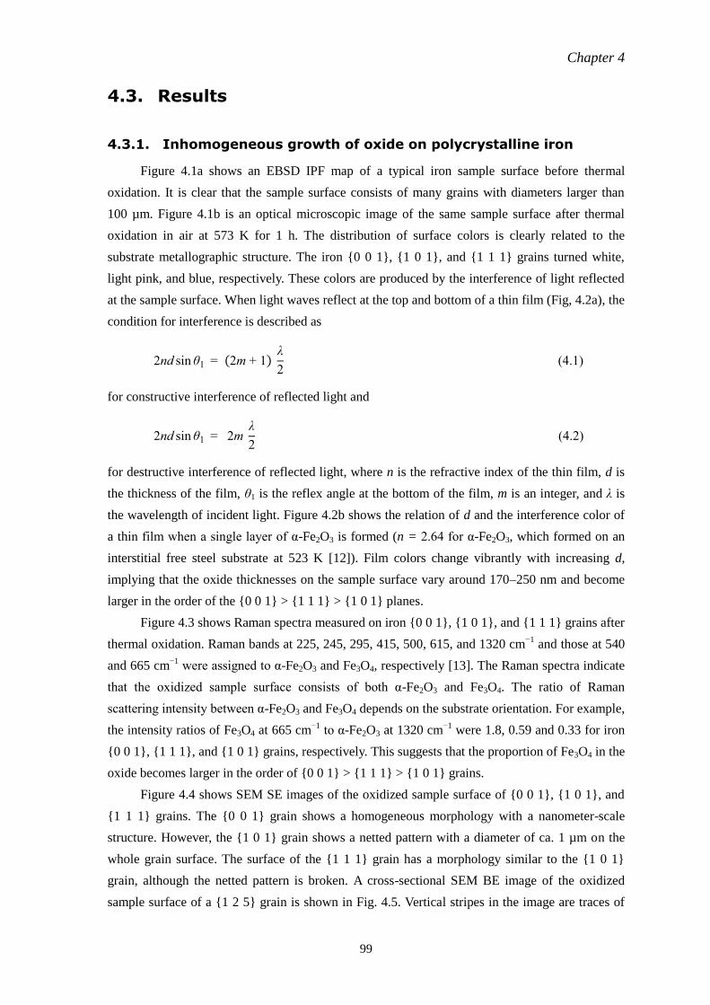
Chapter 4
99
4.3. Results
4.3.1. Inhomogeneous growth of oxide on polycrystalline iron
Figure 4.1a shows an EBSD IPF map of a typical iron sample surface before thermal
oxidation. It is clear that the sample surface consists of many grains with diameters larger than
100 µm. Figure 4.1b is an optical microscopic image of the same sample surface after thermal
oxidation in air at 573 K for 1 h. The distribution of surface colors is clearly related to the
substrate metallographic structure. The iron {0 0 1}, {1 0 1}, and {1 1 1} grains turned white,
light pink, and blue, respectively. These colors are produced by the interference of light reflected
at the sample surface. When light waves reflect at the top and bottom of a thin film (Fig, 4.2a), the
condition for interference is described as
2nd sin θ1 = (2m + 1) λ
2 (4.1)
for constructive interference of reflected light and
2nd sin θ1 = 2m λ
2 (4.2)
for destructive interference of reflected light, where n is the refractive index of the thin film, d is
the thickness of the film, θ1 is the reflex angle at the bottom of the film, m is an integer, and λ is
the wavelength of incident light. Figure 4.2b shows the relation of d and the interference color of
a thin film when a single layer of α-Fe2O3 is formed (n = 2.64 for α-Fe2O3, which formed on an
interstitial free steel substrate at 523 K [12]). Film colors change vibrantly with increasing d,
implying that the oxide thicknesses on the sample surface vary around 170–250 nm and become
larger in the order of the {0 0 1} > {1 1 1} > {1 0 1} planes.
Figure 4.3 shows Raman spectra measured on iron {0 0 1}, {1 0 1}, and {1 1 1} grains after
thermal oxidation. Raman bands at 225, 245, 295, 415, 500, 615, and 1320 cm−1
and those at 540
and 665 cm−1
were assigned to α-Fe2O3 and Fe3O4, respectively [13]. The Raman spectra indicate
that the oxidized sample surface consists of both α-Fe2O3 and Fe3O4. The ratio of Raman
scattering intensity between α-Fe2O3 and Fe3O4 depends on the substrate orientation. For example,
the intensity ratios of Fe3O4 at 665 cm−1
to α-Fe2O3 at 1320 cm−1
were 1.8, 0.59 and 0.33 for iron
{0 0 1}, {1 1 1}, and {1 0 1} grains, respectively. This suggests that the proportion of Fe3O4 in the
oxide becomes larger in the order of {0 0 1} > {1 1 1} > {1 0 1} grains.
Figure 4.4 shows SEM SE images of the oxidized sample surface of {0 0 1}, {1 0 1}, and
{1 1 1} grains. The {0 0 1} grain shows a homogeneous morphology with a nanometer-scale
structure. However, the {1 0 1} grain shows a netted pattern with a diameter of ca. 1 µm on the
whole grain surface. The surface of the {1 1 1} grain has a morphology similar to the {1 0 1}
grain, although the netted pattern is broken. A cross-sectional SEM BE image of the oxidized
sample surface of a {1 2 5} grain is shown in Fig. 4.5. Vertical stripes in the image are traces of
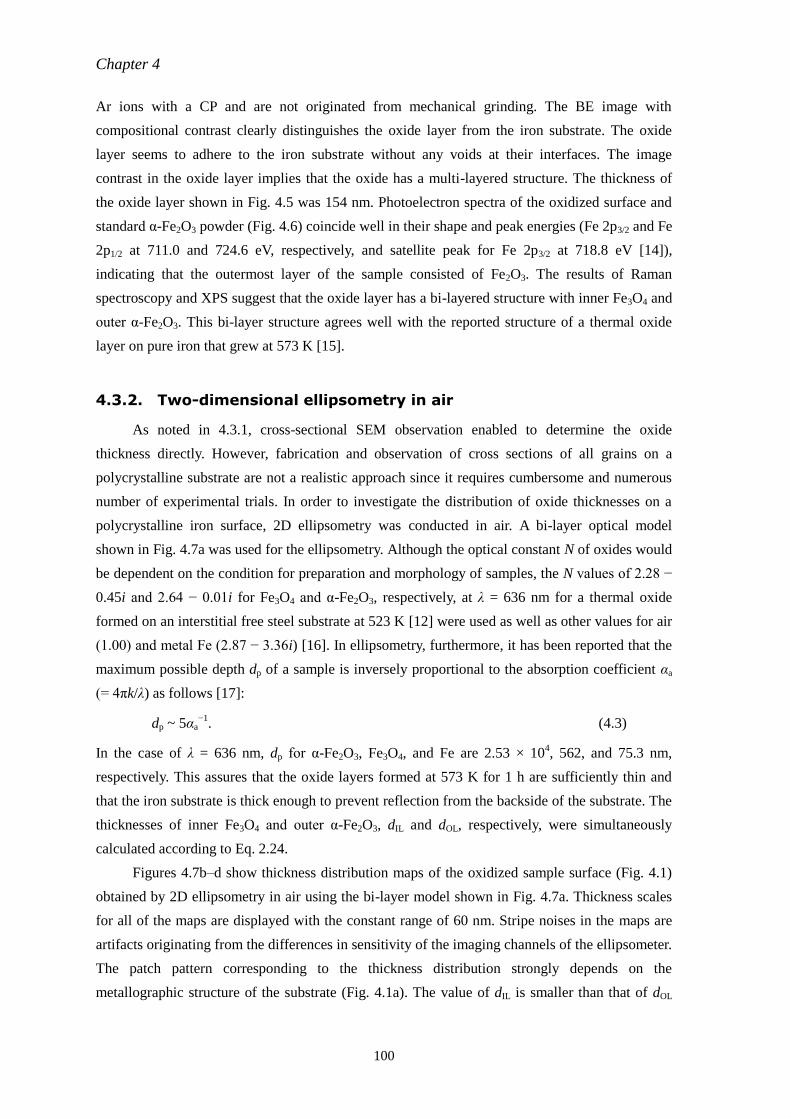
Chapter 4
100
Ar ions with a CP and are not originated from mechanical grinding. The BE image with
compositional contrast clearly distinguishes the oxide layer from the iron substrate. The oxide
layer seems to adhere to the iron substrate without any voids at their interfaces. The image
contrast in the oxide layer implies that the oxide has a multi-layered structure. The thickness of
the oxide layer shown in Fig. 4.5 was 154 nm. Photoelectron spectra of the oxidized surface and
standard α-Fe2O3 powder (Fig. 4.6) coincide well in their shape and peak energies (Fe 2p3/2 and Fe
2p1/2 at 711.0 and 724.6 eV, respectively, and satellite peak for Fe 2p3/2 at 718.8 eV [14]),
indicating that the outermost layer of the sample consisted of Fe2O3. The results of Raman
spectroscopy and XPS suggest that the oxide layer has a bi-layered structure with inner Fe3O4 and
outer α-Fe2O3. This bi-layer structure agrees well with the reported structure of a thermal oxide
layer on pure iron that grew at 573 K [15].
4.3.2. Two-dimensional ellipsometry in air
As noted in 4.3.1, cross-sectional SEM observation enabled to determine the oxide
thickness directly. However, fabrication and observation of cross sections of all grains on a
polycrystalline substrate are not a realistic approach since it requires cumbersome and numerous
number of experimental trials. In order to investigate the distribution of oxide thicknesses on a
polycrystalline iron surface, 2D ellipsometry was conducted in air. A bi-layer optical model
shown in Fig. 4.7a was used for the ellipsometry. Although the optical constant N of oxides would
be dependent on the condition for preparation and morphology of samples, the N values of 2.28 −
0.45i and 2.64 − 0.01i for Fe3O4 and α-Fe2O3, respectively, at λ = 636 nm for a thermal oxide
formed on an interstitial free steel substrate at 523 K [12] were used as well as other values for air
(1.00) and metal Fe (2.87 − 3.36i) [16]. In ellipsometry, furthermore, it has been reported that the
maximum possible depth dp of a sample is inversely proportional to the absorption coefficient αa
(= 4πk/λ) as follows [17]:
dp ~ 5αa−1
. (4.3)
In the case of λ = 636 nm, dp for α-Fe2O3, Fe3O4, and Fe are 2.53 × 10⁴, 562, and 75.3 nm,
respectively. This assures that the oxide layers formed at 573 K for 1 h are sufficiently thin and
that the iron substrate is thick enough to prevent reflection from the backside of the substrate. The
thicknesses of inner Fe3O4 and outer α-Fe2O3, dIL and dOL, respectively, were simultaneously
calculated according to Eq. 2.24.
Figures 4.7b–d show thickness distribution maps of the oxidized sample surface (Fig. 4.1)
obtained by 2D ellipsometry in air using the bi-layer model shown in Fig. 4.7a. Thickness scales
for all of the maps are displayed with the constant range of 60 nm. Stripe noises in the maps are
artifacts originating from the differences in sensitivity of the imaging channels of the ellipsometer.
The patch pattern corresponding to the thickness distribution strongly depends on the
metallographic structure of the substrate (Fig. 4.1a). The value of dIL is smaller than that of dOL
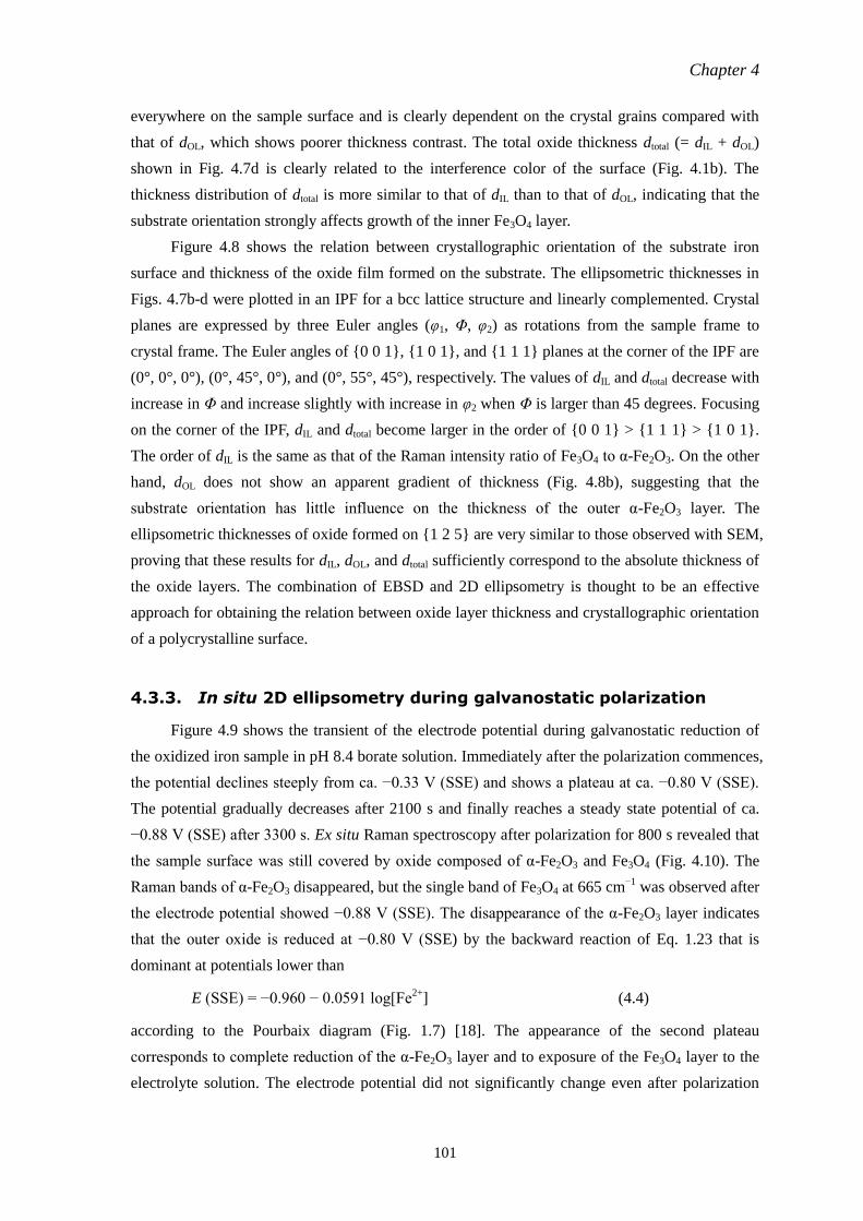
Chapter 4
101
everywhere on the sample surface and is clearly dependent on the crystal grains compared with
that of dOL, which shows poorer thickness contrast. The total oxide thickness dtotal (= dIL + dOL)
shown in Fig. 4.7d is clearly related to the interference color of the surface (Fig. 4.1b). The
thickness distribution of dtotal is more similar to that of dIL than to that of dOL, indicating that the
substrate orientation strongly affects growth of the inner Fe3O4 layer.
Figure 4.8 shows the relation between crystallographic orientation of the substrate iron
surface and thickness of the oxide film formed on the substrate. The ellipsometric thicknesses in
Figs. 4.7b-d were plotted in an IPF for a bcc lattice structure and linearly complemented. Crystal
planes are expressed by three Euler angles (φ1, Φ, φ2) as rotations from the sample frame to
crystal frame. The Euler angles of {0 0 1}, {1 0 1}, and {1 1 1} planes at the corner of the IPF are
(0°, 0°, 0°), (0°, 45°, 0°), and (0°, 55°, 45°), respectively. The values of dIL and dtotal decrease with
increase in Φ and increase slightly with increase in φ2 when Φ is larger than 45 degrees. Focusing
on the corner of the IPF, dIL and dtotal become larger in the order of {0 0 1} > {1 1 1} > {1 0 1}.
The order of dIL is the same as that of the Raman intensity ratio of Fe3O4 to α-Fe2O3. On the other
hand, dOL does not show an apparent gradient of thickness (Fig. 4.8b), suggesting that the
substrate orientation has little influence on the thickness of the outer α-Fe2O3 layer. The
ellipsometric thicknesses of oxide formed on {1 2 5} are very similar to those observed with SEM,
proving that these results for dIL, dOL, and dtotal sufficiently correspond to the absolute thickness of
the oxide layers. The combination of EBSD and 2D ellipsometry is thought to be an effective
approach for obtaining the relation between oxide layer thickness and crystallographic orientation
of a polycrystalline surface.
4.3.3. In situ 2D ellipsometry during galvanostatic polarization
Figure 4.9 shows the transient of the electrode potential during galvanostatic reduction of
the oxidized iron sample in pH 8.4 borate solution. Immediately after the polarization commences,
the potential declines steeply from ca. −0.33 V (SSE) and shows a plateau at ca. −0.80 V (SSE).
The potential gradually decreases after 2100 s and finally reaches a steady state potential of ca.
−0.88 V (SSE) after 3300 s. Ex situ Raman spectroscopy after polarization for 800 s revealed that
the sample surface was still covered by oxide composed of α-Fe2O3 and Fe3O4 (Fig. 4.10). The
Raman bands of α-Fe2O3 disappeared, but the single band of Fe3O4 at 665 cm−1
was observed after
the electrode potential showed −0.88 V (SSE). The disappearance of the α-Fe2O3 layer indicates
that the outer oxide is reduced at −0.80 V (SSE) by the backward reaction of Eq. 1.23 that is
dominant at potentials lower than
E (SSE) = −0.960 − 0.0591 log[Fe2+
] (4.4)
according to the Pourbaix diagram (Fig. 1.7) [18]. The appearance of the second plateau
corresponds to complete reduction of the α-Fe2O3 layer and to exposure of the Fe3O4 layer to the
electrolyte solution. The electrode potential did not significantly change even after polarization
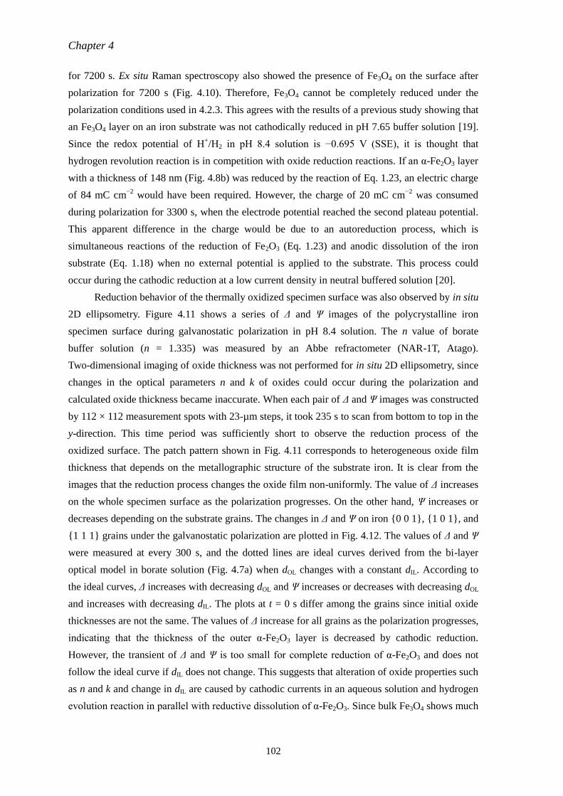
Chapter 4
102
for 7200 s. Ex situ Raman spectroscopy also showed the presence of Fe3O4 on the surface after
polarization for 7200 s (Fig. 4.10). Therefore, Fe3O4 cannot be completely reduced under the
polarization conditions used in 4.2.3. This agrees with the results of a previous study showing that
an Fe3O4 layer on an iron substrate was not cathodically reduced in pH 7.65 buffer solution [19].
Since the redox potential of H+/H2 in pH 8.4 solution is −0.695 V (SSE), it is thought that
hydrogen revolution reaction is in competition with oxide reduction reactions. If an α-Fe2O3 layer
with a thickness of 148 nm (Fig. 4.8b) was reduced by the reaction of Eq. 1.23, an electric charge
of 84 mC cm−2
would have been required. However, the charge of 20 mC cm−2
was consumed
during polarization for 3300 s, when the electrode potential reached the second plateau potential.
This apparent difference in the charge would be due to an autoreduction process, which is
simultaneous reactions of the reduction of Fe2O3 (Eq. 1.23) and anodic dissolution of the iron
substrate (Eq. 1.18) when no external potential is applied to the substrate. This process could
occur during the cathodic reduction at a low current density in neutral buffered solution [20].
Reduction behavior of the thermally oxidized specimen surface was also observed by in situ
2D ellipsometry. Figure 4.11 shows a series of Δ and Ψ images of the polycrystalline iron
specimen surface during galvanostatic polarization in pH 8.4 solution. The n value of borate
buffer solution (n = 1.335) was measured by an Abbe refractometer (NAR-1T, Atago).
Two-dimensional imaging of oxide thickness was not performed for in situ 2D ellipsometry, since
changes in the optical parameters n and k of oxides could occur during the polarization and
calculated oxide thickness became inaccurate. When each pair of Δ and Ψ images was constructed
by 112 × 112 measurement spots with 23-µm steps, it took 235 s to scan from bottom to top in the
y-direction. This time period was sufficiently short to observe the reduction process of the
oxidized surface. The patch pattern shown in Fig. 4.11 corresponds to heterogeneous oxide film
thickness that depends on the metallographic structure of the substrate iron. It is clear from the
images that the reduction process changes the oxide film non-uniformly. The value of Δ increases
on the whole specimen surface as the polarization progresses. On the other hand, Ψ increases or
decreases depending on the substrate grains. The changes in Δ and Ψ on iron {0 0 1}, {1 0 1}, and
{1 1 1} grains under the galvanostatic polarization are plotted in Fig. 4.12. The values of Δ and Ψ
were measured at every 300 s, and the dotted lines are ideal curves derived from the bi-layer
optical model in borate solution (Fig. 4.7a) when dOL changes with a constant dIL. According to
the ideal curves, Δ increases with decreasing dOL and Ψ increases or decreases with decreasing dOL
and increases with decreasing dIL. The plots at t = 0 s differ among the grains since initial oxide
thicknesses are not the same. The values of Δ increase for all grains as the polarization progresses,
indicating that the thickness of the outer α-Fe2O3 layer is decreased by cathodic reduction.
However, the transient of Δ and Ψ is too small for complete reduction of α-Fe2O3 and does not
follow the ideal curve if dIL does not change. This suggests that alteration of oxide properties such
as n and k and change in dIL are caused by cathodic currents in an aqueous solution and hydrogen
evolution reaction in parallel with reductive dissolution of α-Fe2O3. Since bulk Fe3O4 shows much
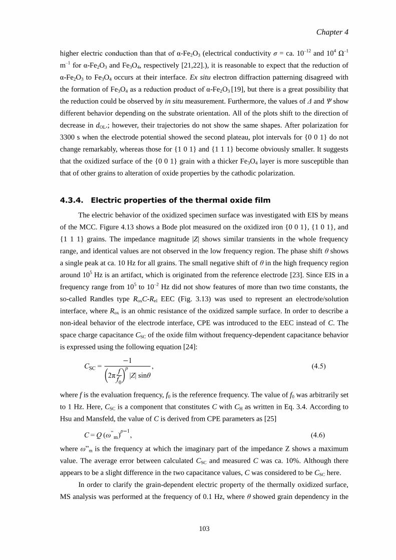
Chapter 4
103
higher electric conduction than that of α-Fe2O3 (electrical conductivity σ = ca. 10–12
and 104 Ω
–1
m–1
for α-Fe2O3 and Fe3O4, respectively [21,22].), it is reasonable to expect that the reduction of
α-Fe2O3 to Fe3O4 occurs at their interface. Ex situ electron diffraction patterning disagreed with
the formation of Fe3O4 as a reduction product of α-Fe2O3 [19], but there is a great possibility that
the reduction could be observed by in situ measurement. Furthermore, the values of Δ and Ψ show
different behavior depending on the substrate orientation. All of the plots shift to the direction of
decrease in dOL.; however, their trajectories do not show the same shapes. After polarization for
3300 s when the electrode potential showed the second plateau, plot intervals for {0 0 1} do not
change remarkably, whereas those for {1 0 1} and {1 1 1} become obviously smaller. It suggests
that the oxidized surface of the {0 0 1} grain with a thicker Fe3O4 layer is more susceptible than
that of other grains to alteration of oxide properties by the cathodic polarization.
4.3.4. Electric properties of the thermal oxide film
The electric behavior of the oxidized specimen surface was investigated with EIS by means
of the MCC. Figure 4.13 shows a Bode plot measured on the oxidized iron {0 0 1}, {1 0 1}, and
{1 1 1} grains. The impedance magnitude |Z| shows similar transients in the whole frequency
range, and identical values are not observed in the low frequency region. The phase shift θ shows
a single peak at ca. 10 Hz for all grains. The small negative shift of θ in the high frequency region
around 105 Hz is an artifact, which is originated from the reference electrode [23]. Since EIS in a
frequency range from 105 to 10
–2 Hz did not show features of more than two time constants, the
so-called Randles type RoxC-Rel EEC (Fig. 3.13) was used to represent an electrode/solution
interface, where Rox is an ohmic resistance of the oxidized sample surface. In order to describe a
non-ideal behavior of the electrode interface, CPE was introduced to the EEC instead of C. The
space charge capacitance CSC of the oxide film without frequency-dependent capacitance behavior
is expressed using the following equation [24]:
CSC = −1
(2πff0
)p
|Z| sinθ
, (4.5)
where f is the evaluation frequency, f0 is the reference frequency. The value of f0 was arbitrarily set
to 1 Hz. Here, CSC is a component that constitutes C with CH as written in Eq. 3.4. According to
Hsu and Mansfeld, the value of C is derived from CPE parameters as [25]
C = Q (ω”m)
p−1, (4.6)
where ω”m is the frequency at which the imaginary part of the impedance Z shows a maximum
value. The average error between calculated CSC and measured C was ca. 10%. Although there
appears to be a slight difference in the two capacitance values, C was considered to be CSC here.
In order to clarify the grain-dependent electric property of the thermally oxidized surface,
MS analysis was performed at the frequency of 0.1 Hz, where θ showed grain dependency in the
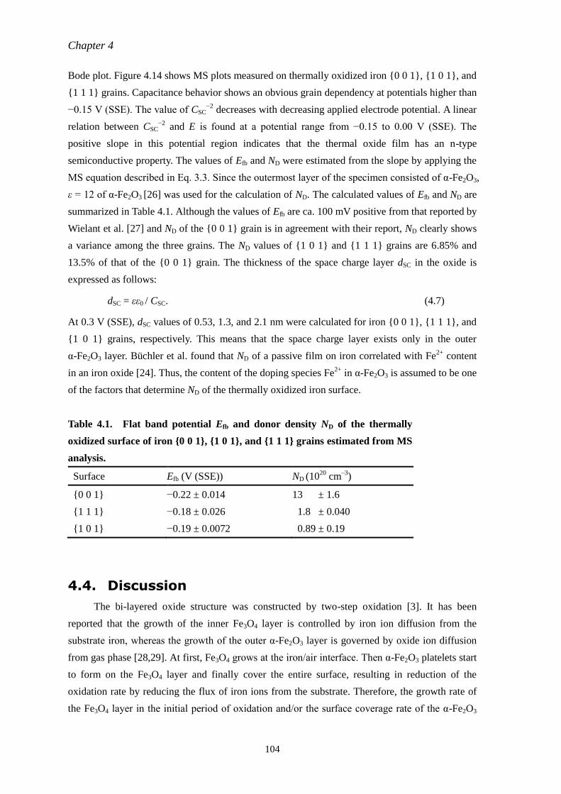
Chapter 4
104
Bode plot. Figure 4.14 shows MS plots measured on thermally oxidized iron {0 0 1}, {1 0 1}, and
{1 1 1} grains. Capacitance behavior shows an obvious grain dependency at potentials higher than
−0.15 V (SSE). The value of CSC−2
decreases with decreasing applied electrode potential. A linear
relation between CSC−2
and E is found at a potential range from −0.15 to 0.00 V (SSE). The
positive slope in this potential region indicates that the thermal oxide film has an n-type
semiconductive property. The values of Efb and ND were estimated from the slope by applying the
MS equation described in Eq. 3.3. Since the outermost layer of the specimen consisted of α-Fe2O3,
ε = 12 of α-Fe2O3 [26] was used for the calculation of ND. The calculated values of Efb and ND are
summarized in Table 4.1. Although the values of Efb are ca. 100 mV positive from that reported by
Wielant et al. [27] and ND of the {0 0 1} grain is in agreement with their report, ND clearly shows
a variance among the three grains. The ND values of {1 0 1} and {1 1 1} grains are 6.85% and
13.5% of that of the {0 0 1} grain. The thickness of the space charge layer dSC in the oxide is
expressed as follows:
dSC = εε0 / CSC. (4.7)
At 0.3 V (SSE), dSC values of 0.53, 1.3, and 2.1 nm were calculated for iron {0 0 1}, {1 1 1}, and
{1 0 1} grains, respectively. This means that the space charge layer exists only in the outer
α-Fe2O3 layer. Büchler et al. found that ND of a passive film on iron correlated with Fe2+
content
in an iron oxide [24]. Thus, the content of the doping species Fe2+
in α-Fe2O3 is assumed to be one
of the factors that determine ND of the thermally oxidized iron surface.
Table 4.1. Flat band potential Efb and donor density ND of the thermally
oxidized surface of iron {0 0 1}, {1 0 1}, and {1 1 1} grains estimated from MS
analysis.
Surface Efb (V (SSE)) ND (1020
cm–3
)
{0 0 1} −0.22 ± 0.014 13 ± 1.6
{1 1 1} −0.18 ± 0.026 1.8 ± 0.040
{1 0 1} −0.19 ± 0.0072 0.89 ± 0.19
4.4. Discussion
The bi-layered oxide structure was constructed by two-step oxidation [3]. It has been
reported that the growth of the inner Fe3O4 layer is controlled by iron ion diffusion from the
substrate iron, whereas the growth of the outer α-Fe2O3 layer is governed by oxide ion diffusion
from gas phase [28,29]. At first, Fe3O4 grows at the iron/air interface. Then α-Fe2O3 platelets start
to form on the Fe3O4 layer and finally cover the entire surface, resulting in reduction of the
oxidation rate by reducing the flux of iron ions from the substrate. Therefore, the growth rate of
the Fe3O4 layer in the initial period of oxidation and/or the surface coverage rate of the α-Fe2O3
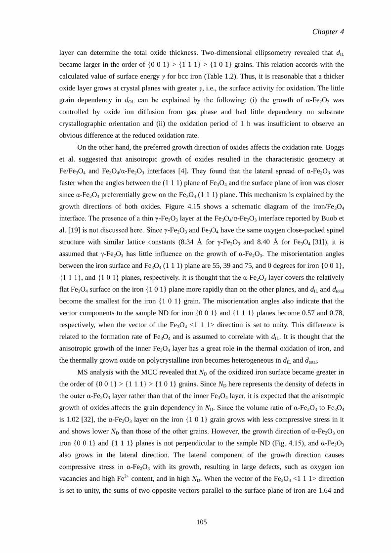
Chapter 4
105
layer can determine the total oxide thickness. Two-dimensional ellipsometry revealed that dIL
became larger in the order of {0 0 1} > {1 1 1} > {1 0 1} grains. This relation accords with the
calculated value of surface energy γ for bcc iron (Table 1.2). Thus, it is reasonable that a thicker
oxide layer grows at crystal planes with greater γ, i.e., the surface activity for oxidation. The little
grain dependency in dOL can be explained by the following: (i) the growth of α-Fe2O3 was
controlled by oxide ion diffusion from gas phase and had little dependency on substrate
crystallographic orientation and (ii) the oxidation period of 1 h was insufficient to observe an
obvious difference at the reduced oxidation rate.
On the other hand, the preferred growth direction of oxides affects the oxidation rate. Boggs
et al. suggested that anisotropic growth of oxides resulted in the characteristic geometry at
Fe/Fe3O4 and Fe3O4/α-Fe2O3 interfaces [4]. They found that the lateral spread of α-Fe2O3 was
faster when the angles between the (1 1 1) plane of Fe3O4 and the surface plane of iron was closer
since α-Fe2O3 preferentially grew on the Fe3O4 (1 1 1) plane. This mechanism is explained by the
growth directions of both oxides. Figure 4.15 shows a schematic diagram of the iron/Fe3O4
interface. The presence of a thin γ-Fe2O3 layer at the Fe3O4/α-Fe2O3 interface reported by Buob et
al. [19] is not discussed here. Since γ-Fe2O3 and Fe3O4 have the same oxygen close-packed spinel
structure with similar lattice constants (8.34 Å for γ-Fe2O3 and 8.40 Å for Fe3O4 [31]), it is
assumed that γ-Fe2O3 has little influence on the growth of α-Fe2O3. The misorientation angles
between the iron surface and Fe3O4 (1 1 1) plane are 55, 39 and 75, and 0 degrees for iron {0 0 1},
{1 1 1}, and {1 0 1} planes, respectively. It is thought that the α-Fe2O3 layer covers the relatively
flat Fe3O4 surface on the iron {1 0 1} plane more rapidly than on the other planes, and dIL and dtotal
become the smallest for the iron {1 0 1} grain. The misorientation angles also indicate that the
vector components to the sample ND for iron {0 0 1} and {1 1 1} planes become 0.57 and 0.78,
respectively, when the vector of the Fe3O4 <1 1 1> direction is set to unity. This difference is
related to the formation rate of Fe3O4 and is assumed to correlate with dIL. It is thought that the
anisotropic growth of the inner Fe3O4 layer has a great role in the thermal oxidation of iron, and
the thermally grown oxide on polycrystalline iron becomes heterogeneous in dIL and dtotal.
MS analysis with the MCC revealed that ND of the oxidized iron surface became greater in
the order of {0 0 1} > {1 1 1} > {1 0 1} grains. Since ND here represents the density of defects in
the outer α-Fe2O3 layer rather than that of the inner Fe3O4 layer, it is expected that the anisotropic
growth of oxides affects the grain dependency in ND. Since the volume ratio of α-Fe2O3 to Fe3O4
is 1.02 [32], the α-Fe2O3 layer on the iron {1 0 1} grain grows with less compressive stress in it
and shows lower ND than those of the other grains. However, the growth direction of α-Fe2O3 on
iron {0 0 1} and {1 1 1} planes is not perpendicular to the sample ND (Fig. 4.15), and α-Fe2O3
also grows in the lateral direction. The lateral component of the growth direction causes
compressive stress in α-Fe2O3 with its growth, resulting in large defects, such as oxygen ion
vacancies and high Fe2+
content, and in high ND. When the vector of the Fe3O4 <1 1 1> direction
is set to unity, the sums of two opposite vectors parallel to the surface plane of iron are 1.64 and
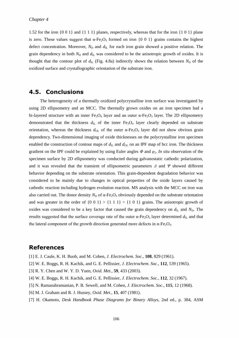
Chapter 4
106
1.52 for the iron {0 0 1} and {1 1 1} planes, respectively, whereas that for the iron {1 0 1} plane
is zero. These values suggest that α-Fe2O3 formed on iron {0 0 1} grains contains the highest
defect concentration. Moreover, ND and dIL for each iron grain showed a positive relation. The
grain dependency in both ND and dIL was considered to be the anisotropic growth of oxides. It is
thought that the contour plot of dIL (Fig. 4.8a) indirectly shows the relation between ND of the
oxidized surface and crystallographic orientation of the substrate iron.
4.5. Conclusions
The heterogeneity of a thermally oxidized polycrystalline iron surface was investigated by
using 2D ellipsometry and an MCC. The thermally grown oxides on an iron specimen had a
bi-layered structure with an inner Fe3O4 layer and an outer α-Fe2O3 layer. The 2D ellipsometry
demonstrated that the thickness dIL of the inner Fe3O4 layer clearly depended on substrate
orientation, whereas the thickness dOL of the outer α-Fe2O3 layer did not show obvious grain
dependency. Two-dimensional imaging of oxide thicknesses on the polycrystalline iron specimen
enabled the construction of contour maps of dIL and dOL on an IPF map of bcc iron. The thickness
gradient on the IPF could be explained by using Euler angles Φ and φ2. In situ observation of the
specimen surface by 2D ellipsometry was conducted during galvanostatic cathodic polarization,
and it was revealed that the transient of ellipsometric parameters Δ and Ψ showed different
behavior depending on the substrate orientation. This grain-dependent degradation behavior was
considered to be mainly due to changes in optical properties of the oxide layers caused by
cathodic reaction including hydrogen evolution reaction. MS analysis with the MCC on iron was
also carried out. The donor density ND of α-Fe2O3 obviously depended on the substrate orientation
and was greater in the order of {0 0 1} > {1 1 1} > {1 0 1} grains. The anisotropic growth of
oxides was considered to be a key factor that caused the grain dependency on dIL and ND. The
results suggested that the surface coverage rate of the outer α-Fe2O3 layer determined dIL and that
the lateral component of the growth direction generated more defects in α-Fe2O3.
References
[1] E. J. Caule, K. H. Buob, and M. Cohen, J. Electrochem. Soc., 108, 829 (1961).
[2] W. E. Boggs, R. H. Kachik, and G. E. Pellissier, J. Electrochem. Soc., 112, 539 (1965).
[3] R. Y. Chen and W. Y. D. Yuen, Oxid. Met., 59, 433 (2003).
[4] W. E. Boggs, R. H. Kachik, and G. E. Pellissier, J. Electrochem. Soc., 112, 32 (1967).
[5] N. Ramasubramanian, P. B. Sewell, and M. Cohen, J. Electrochem. Soc., 115, 12 (1968).
[6] M. J. Graham and R. J. Hussey, Oxid. Met., 15, 407 (1981).
[7] H. Okamoto, Desk Handbook Phase Diagrams for Binary Alloys, 2nd ed., p. 384, ASM
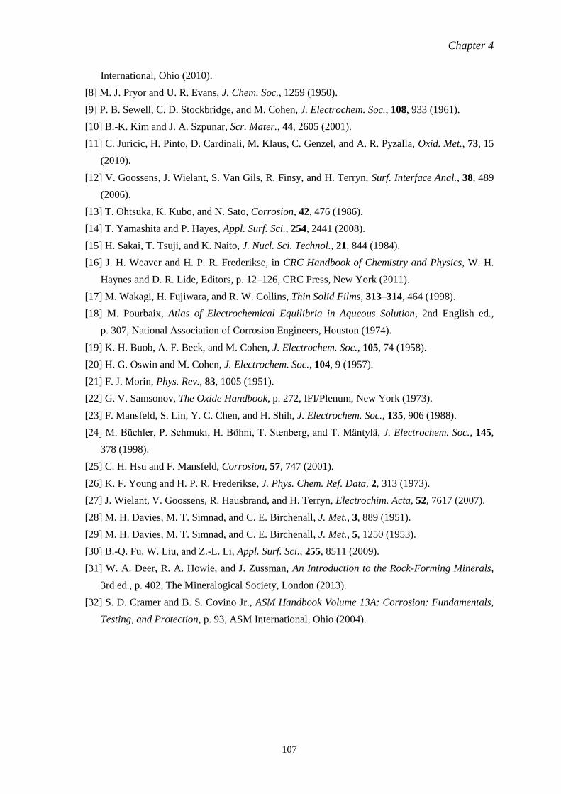
Chapter 4
107
International, Ohio (2010).
[8] M. J. Pryor and U. R. Evans, J. Chem. Soc., 1259 (1950).
[9] P. B. Sewell, C. D. Stockbridge, and M. Cohen, J. Electrochem. Soc., 108, 933 (1961).
[10] B.-K. Kim and J. A. Szpunar, Scr. Mater., 44, 2605 (2001).
[11] C. Juricic, H. Pinto, D. Cardinali, M. Klaus, C. Genzel, and A. R. Pyzalla, Oxid. Met., 73, 15
(2010).
[12] V. Goossens, J. Wielant, S. Van Gils, R. Finsy, and H. Terryn, Surf. Interface Anal., 38, 489
(2006).
[13] T. Ohtsuka, K. Kubo, and N. Sato, Corrosion, 42, 476 (1986).
[14] T. Yamashita and P. Hayes, Appl. Surf. Sci., 254, 2441 (2008).
[15] H. Sakai, T. Tsuji, and K. Naito, J. Nucl. Sci. Technol., 21, 844 (1984).
[16] J. H. Weaver and H. P. R. Frederikse, in CRC Handbook of Chemistry and Physics, W. H.
Haynes and D. R. Lide, Editors, p. 12–126, CRC Press, New York (2011).
[17] M. Wakagi, H. Fujiwara, and R. W. Collins, Thin Solid Films, 313–314, 464 (1998).
[18] M. Pourbaix, Atlas of Electrochemical Equilibria in Aqueous Solution, 2nd English ed.,
p. 307, National Association of Corrosion Engineers, Houston (1974).
[19] K. H. Buob, A. F. Beck, and M. Cohen, J. Electrochem. Soc., 105, 74 (1958).
[20] H. G. Oswin and M. Cohen, J. Electrochem. Soc., 104, 9 (1957).
[21] F. J. Morin, Phys. Rev., 83, 1005 (1951).
[22] G. V. Samsonov, The Oxide Handbook, p. 272, IFI/Plenum, New York (1973).
[23] F. Mansfeld, S. Lin, Y. C. Chen, and H. Shih, J. Electrochem. Soc., 135, 906 (1988).
[24] M. Buchler, P. Schmuki, H. Böhni, T. Stenberg, and T. Mäntylä, J. Electrochem. Soc., 145,
378 (1998).
[25] C. H. Hsu and F. Mansfeld, Corrosion, 57, 747 (2001).
[26] K. F. Young and H. P. R. Frederikse, J. Phys. Chem. Ref. Data, 2, 313 (1973).
[27] J. Wielant, V. Goossens, R. Hausbrand, and H. Terryn, Electrochim. Acta, 52, 7617 (2007).
[28] M. H. Davies, M. T. Simnad, and C. E. Birchenall, J. Met., 3, 889 (1951).
[29] M. H. Davies, M. T. Simnad, and C. E. Birchenall, J. Met., 5, 1250 (1953).
[30] B.-Q. Fu, W. Liu, and Z.-L. Li, Appl. Surf. Sci., 255, 8511 (2009).
[31] W. A. Deer, R. A. Howie, and J. Zussman, An Introduction to the Rock-Forming Minerals,
3rd ed., p. 402, The Mineralogical Society, London (2013).
[32] S. D. Cramer and B. S. Covino Jr., ASM Handbook Volume 13A: Corrosion: Fundamentals,
Testing, and Protection, p. 93, ASM International, Ohio (2004).
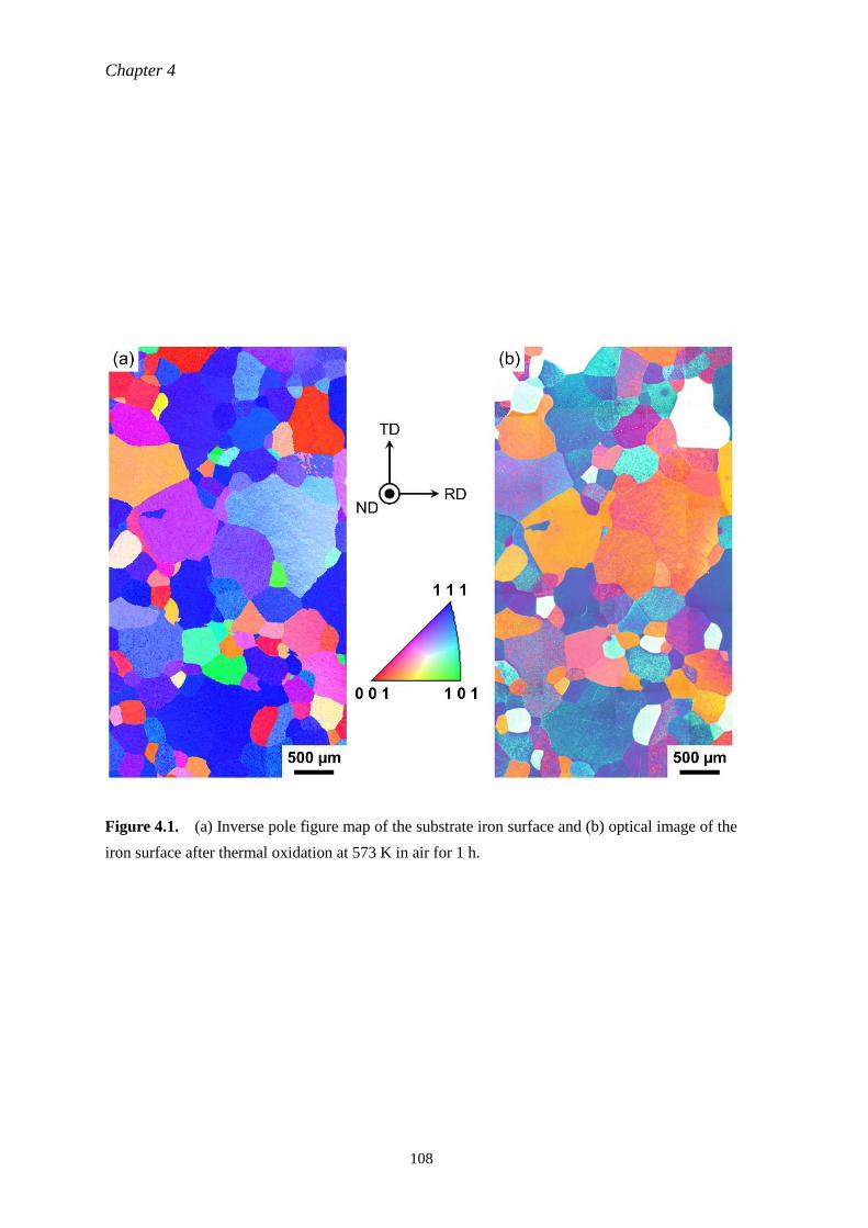
Chapter 4
108
Figure 4.1. (a) Inverse pole figure map of the substrate iron surface and (b) optical image of the
iron surface after thermal oxidation at 573 K in air for 1 h.
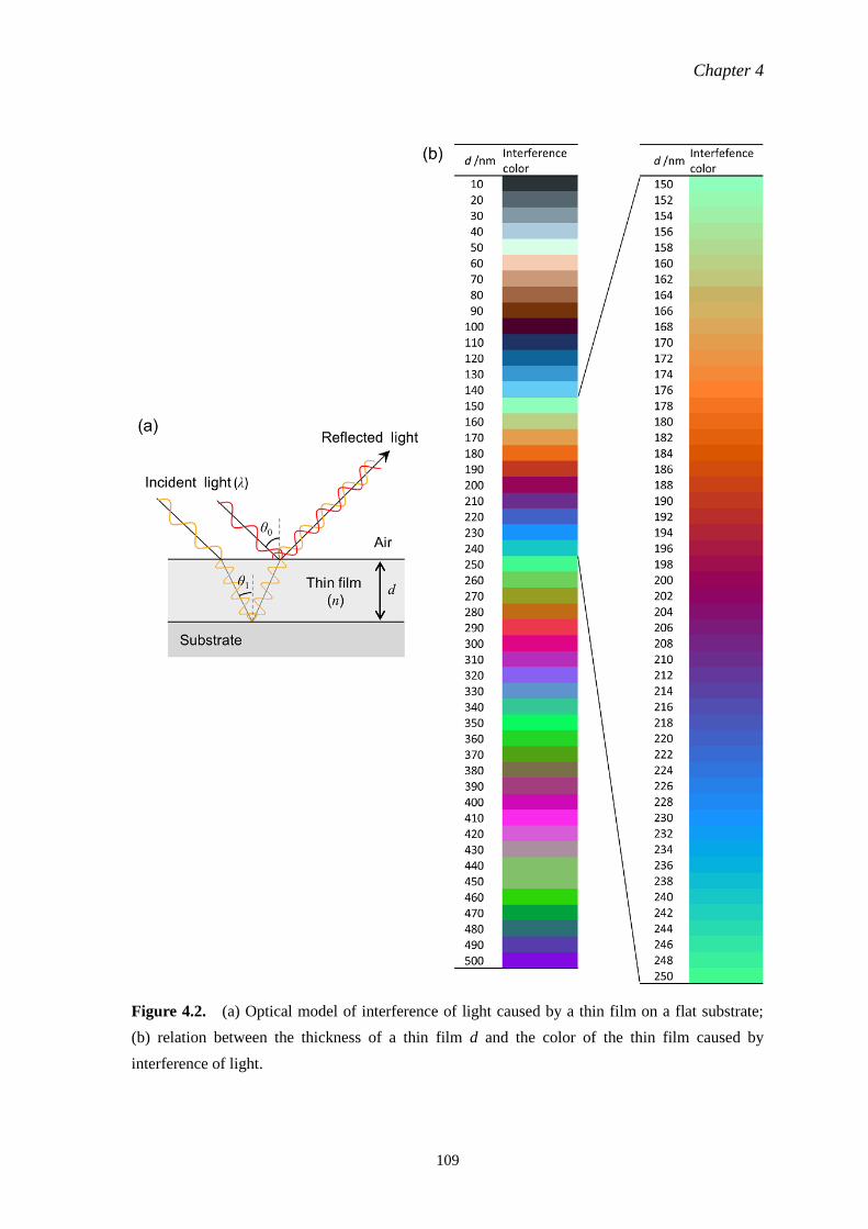
Chapter 4
109
Figure 4.2. (a) Optical model of interference of light caused by a thin film on a flat substrate;
(b) relation between the thickness of a thin film d and the color of the thin film caused by
interference of light.
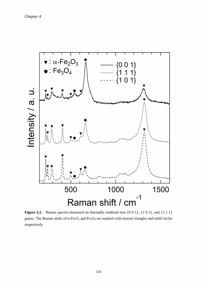
Chapter 4
110
Figure 4.3. Raman spectra measured on thermally oxidized iron {0 0 1}, {1 0 1}, and {1 1 1}
grains. The Raman shifts of α-Fe2O3 and Fe3O4 are marked with inverse triangles and solid circles
respectively.
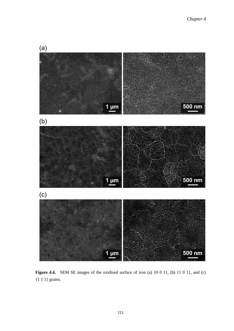
Chapter 4
111
Figure 4.4. SEM SE images of the oxidized surface of iron (a) {0 0 1}, (b) {1 0 1}, and (c)
{1 1 1} grains.
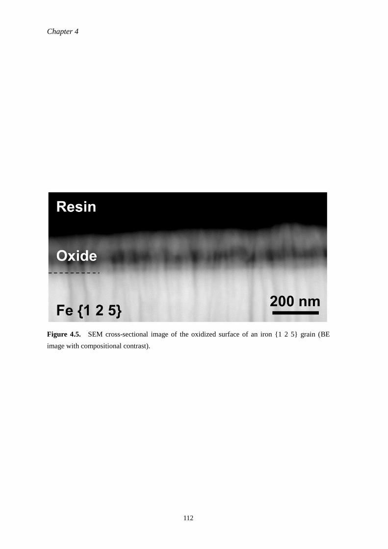
Chapter 4
112
Figure 4.5. SEM cross-sectional image of the oxidized surface of an iron {1 2 5} grain (BE
image with compositional contrast).
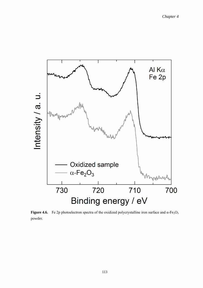
Chapter 4
113
Figure 4.6. Fe 2p photoelectron spectra of the oxidized polycrystalline iron surface and α-Fe2O3
powder.

Chapter 4
114
Figure 4.7. (a) Optical model used for 2D ellipsometry; dIL and dOL, thickness of the inner
Fe3O4 layer and that of the outer α-Fe2O3 layer respectively; (b–d) 2D maps of dIL and dOL, and
total layer thickness dtotal (= dIL + dOL), with these maps showing the same sample surface as that
shown in Fig. 4.1.
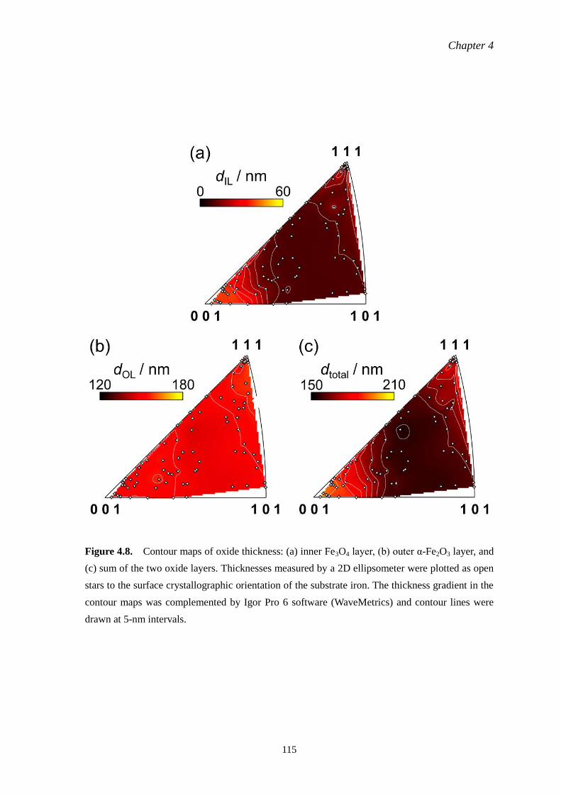
Chapter 4
115
Figure 4.8. Contour maps of oxide thickness: (a) inner Fe3O4 layer, (b) outer α-Fe2O3 layer, and
(c) sum of the two oxide layers. Thicknesses measured by a 2D ellipsometer were plotted as open
stars to the surface crystallographic orientation of the substrate iron. The thickness gradient in the
contour maps was complemented by Igor Pro 6 software (WaveMetrics) and contour lines were
drawn at 5-nm intervals.
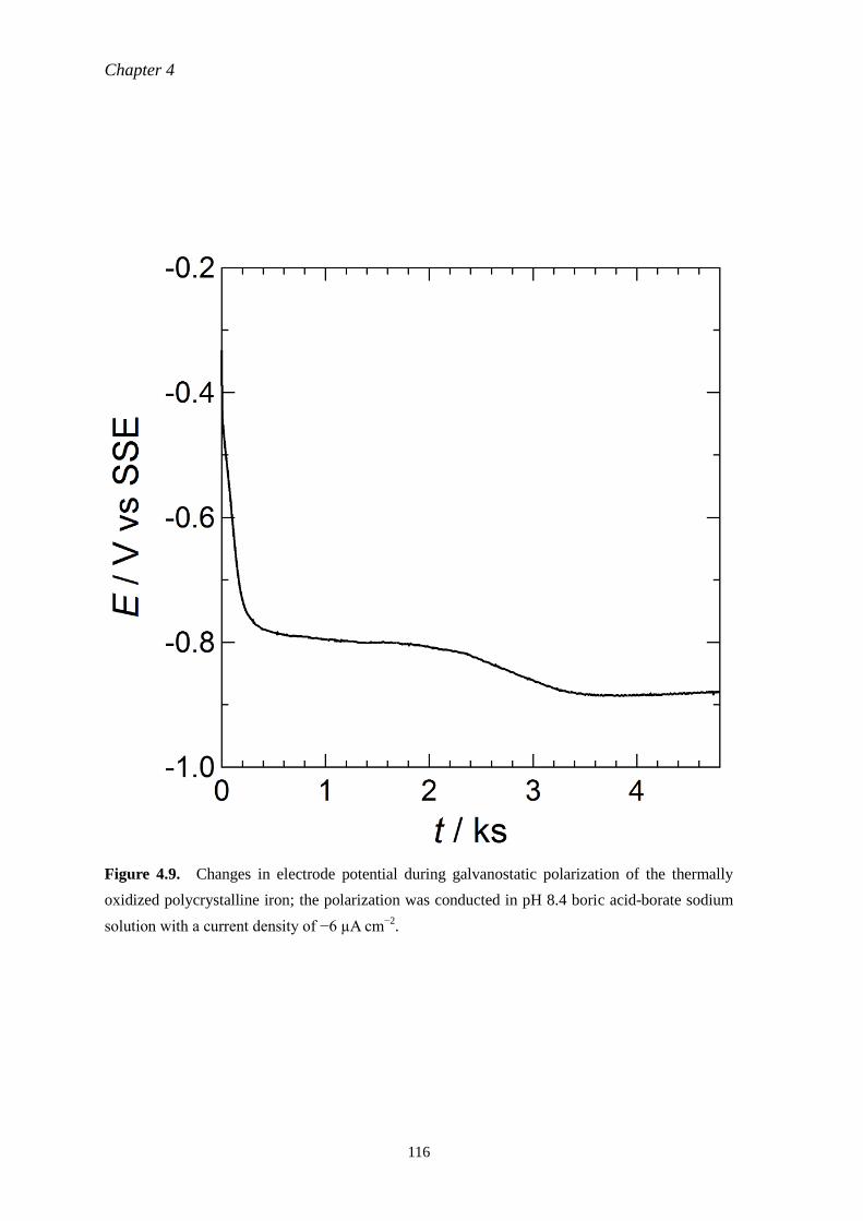
Chapter 4
116
Figure 4.9. Changes in electrode potential during galvanostatic polarization of the thermally
oxidized polycrystalline iron; the polarization was conducted in pH 8.4 boric acid-borate sodium
solution with a current density of −6 µA cm−2
.
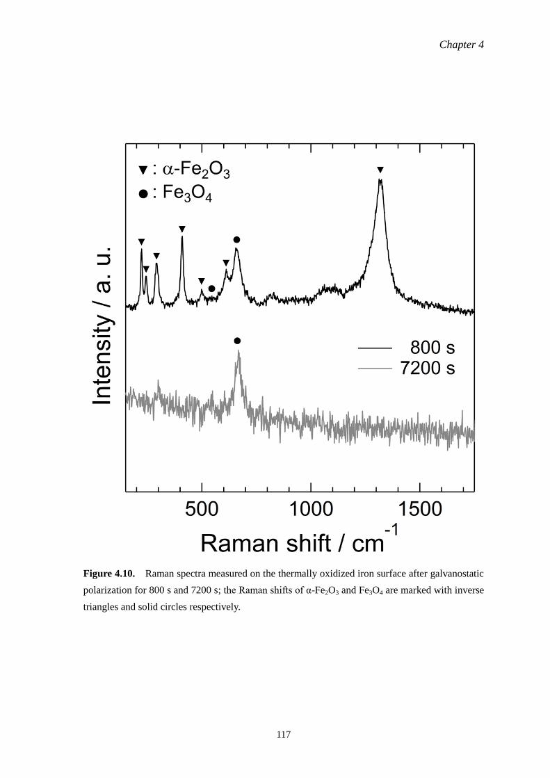
Chapter 4
117
Figure 4.10. Raman spectra measured on the thermally oxidized iron surface after galvanostatic
polarization for 800 s and 7200 s; the Raman shifts of α-Fe2O3 and Fe3O4 are marked with inverse
triangles and solid circles respectively.
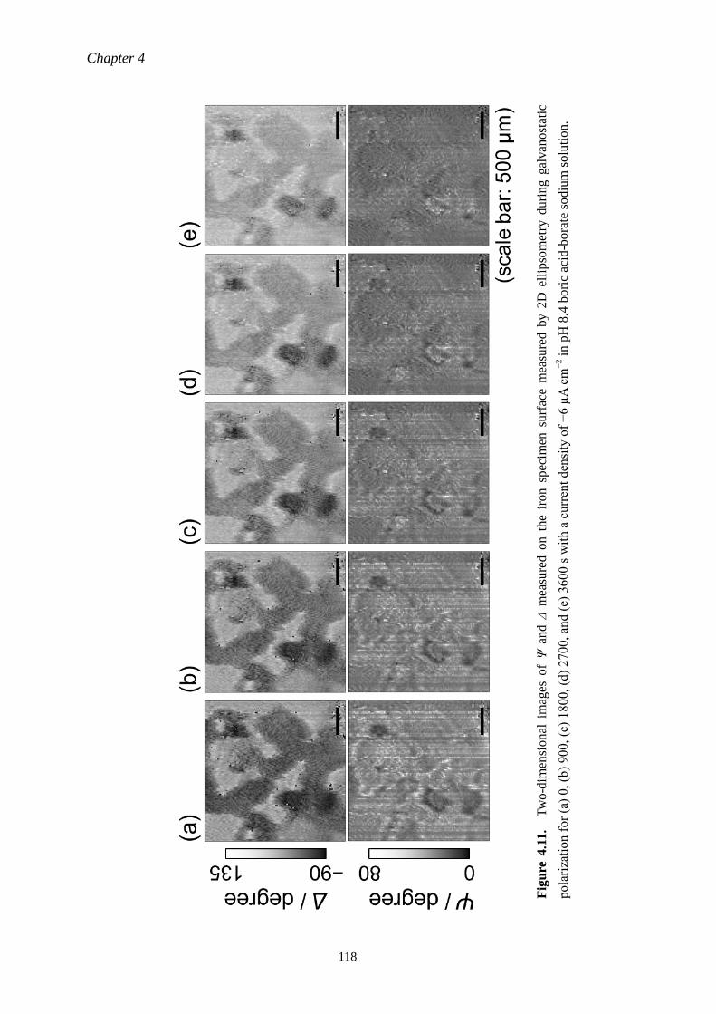
Chapter 4
118
Fig
ure
4.1
1.
T
wo
-dim
ensi
on
al i
mag
es o
f Ψ
and Δ
mea
sure
d o
n t
he
iron s
pec
imen
surf
ace
mea
sure
d b
y 2
D e
llip
som
etry
du
rin
g g
alvan
ost
atic
pola
riza
tio
n f
or
(a)
0, (b
) 90
0, (c
) 1
800,
(d)
2700,
and (
e) 3
600 s
wit
h a
curr
ent
den
sity
of
−6 µ
A c
m−
2 i
n p
H 8
.4 b
ori
c ac
id-b
ora
te s
od
ium
so
luti
on
.
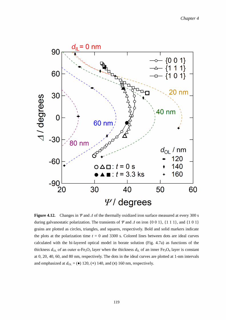
Chapter 4
119
Figure 4.12. Changes in Ψ and Δ of the thermally oxidized iron surface measured at every 300 s
during galvanostatic polarization. The transients of Ψ and Δ on iron {0 0 1}, {1 1 1}, and {1 0 1}
grains are plotted as circles, triangles, and squares, respectively. Bold and solid markers indicate
the plots at the polarization time t = 0 and 3300 s. Colored lines between dots are ideal curves
calculated with the bi-layered optical model in borate solution (Fig. 4.7a) as functions of the
thickness dOL of an outer α-Fe2O3 layer when the thickness dIL of an inner Fe3O4 layer is constant
at 0, 20, 40, 60, and 80 nm, respectively. The dots in the ideal curves are plotted at 1-nm intervals
and emphasized at dOL = (♦) 120, (+) 140, and (x) 160 nm, respectively.
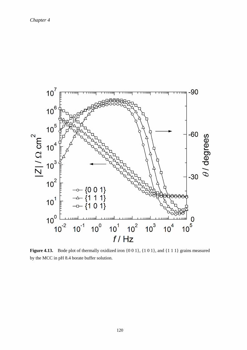
Chapter 4
120
Figure 4.13. Bode plot of thermally oxidized iron {0 0 1}, {1 0 1}, and {1 1 1} grains measured
by the MCC in pH 8.4 borate buffer solution.
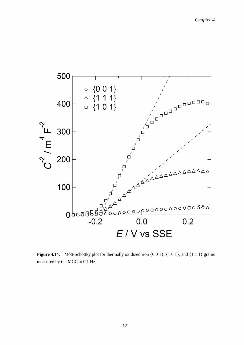
Chapter 4
121
Figure 4.14. Mott-Schottky plot for thermally oxidized iron {0 0 1}, {1 0 1}, and {1 1 1} grains
measured by the MCC at 0.1 Hz.
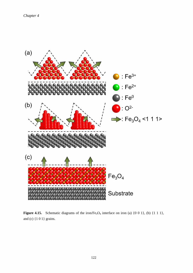
Chapter 4
122
Figure 4.15. Schematic diagrams of the iron/Fe3O4 interface on iron (a) {0 0 1}, (b) {1 1 1},
and (c) {1 0 1} grains.
Chapter 5
123
Chapter 5
Grain-dependency of passive
film formed in neutral borate
solution investigated by MCC
and 2D ellipsometry
5.1. Introduction
As noted in Chapter 1, the structure, thickness, and characteristics of a passive film formed
on iron have been intensively studied in neutral borate buffer solution, in which the dissolution of
the film and/or the substrate into the solution is negligible. However, most previous studies on
passive film have used a polycrystalline electrode, thus overlooking heterogeneous passivation
behavior that might occur on the polycrystalline substrate due to the grain-dependent passivation
that is affected by the various crystallographic orientations of surface grains.
Davenport et al. [1], who conducted in situ XRD, observed that the structure of the passive
film depended on the surface crystallographic orientation. They used single crystals as sample
specimens and explained that the difference in the structure of the passive film was due to the
epitaxial relationship between the film and the substrate. The heterogeneity of the passive film
formed on whole polycrystalline iron surface was examined by Fushimi et al. [2], who performed
SECM in pH 8.4 borate buffer solution. The probe current, which reflected the tunneling current
through the passive film, obviously depended on the substrate grains and the current flowed above
the grain surface oriented to the {1 0 0} plane was less than that above the grain surface oriented
to the {1 1 0} and {1 1 1} planes, indicating that the electronic resistivity of the film differed
among the substrate grains. They ascribed their results largely to the difference in thickness of the
passive films.
As noted above, the heterogeneity of the passive film formed on a polycrystalline iron
surface has been reported. However, the passivation behavior of each grain has not been studied
and the mechanism that leads to the grain dependency of the film remains unclear. In Chapter 3,
grain-dependent passivation in pH 1.3 sulfuric acid was clearly demonstrated with an MCC
technique. In Chapter 4, the heterogeneous thickness distribution and degradation behavior of the
oxide film formed on whole polycrystalline substrate were successfully observed by in situ 2D
ellipsometry. Thus, the combination of these techniques is expected to clarify the precise
Chapter 5
124
mechanism of grain-dependent passivation of polycrystalline iron by examining the passivation
behavior of both single grains and whole surface of a polycrystalline substrate.
In this chapter, the passivation behavior of polycrystalline iron in pH 8.4 borate buffer
solution was investigated by means of in situ 2D ellipsometry and an MCC method. Furthermore,
the electric property of a passive film formed on each grain was evaluated by EIS with the MCC.
5.2. Experimental
5.2.1. In situ 2D ellipsometry
The sample specimen of polycrystalline iron prepared in section 2.1 was mounted on an
epoxy resin holder and placed in an electrochemical cell designed for in situ 2D ellipsometry (Fig.
2.16). At first, a native oxide film that formed on the sample surface was removed by
galvanostatic polarization at −6 µA cm−2
in pH 6.5 borate buffer for 400 s. After the electrolyte
solution was changed to fresh solution of pH 8.4 borate buffer solution, Ecorr was measured for 10
s and followed by potentiodynamic polarization from (Ecorr − 0.05 V) to 1.1 V (SSE) at a potential
sweep rate of 1 mV s−1
or potentiostatic polarization at 0.9 V (SSE) for 24 h. In parallel with the
potentiostatic polarization, in situ 2D ellipsometry was conducted at the polarization periods of 0,
1, 6, 12, and 24 h. The changes in Ψ and Δ were measured during the potentiostatic polarization.
Separately, EIS measurements were taken after the potentiostatic polarization at 0.9 V (SSE) for 1,
6, 12, and 24 h with an ac voltage amplitude of ±10 mV in the frequency range of 105 to 10
−2 Hz.
5.2.2. Micro-electrochemistry
Micro-electrochemical measurements were conducted with an MCC that had a capillary tip
with an inner diameter of 200 µm. The fabrication of the MCC was described in section 2.2. The
tip of the cell had an electrolyte contact area of 3.1 × 10⁻⁴
cm2 on the sample surface. An
electrolyte solution of pH 8.4 borate buffer solution filled the inside of the capillary. The capillary
tip was placed on a grain of the polycrystalline iron sample and potentiostatic polarization was
performed at 0.9 V (SSE) for 1 h. Immediately after potentiostatic polarization, EIS was
performed at 0.9 V (SSE) with an ac voltage amplitude of ±10 mV with a frequency range of 105
to 10−2
Hz. Separately, MS analysis was performed immediately after the potentiostatic
polarization in a potential range from 0.4 to −0.4 V (SSE) with an ac voltage of ±5 mV at a
frequency of 10 Hz.
5.2.3. Characterization of the passive film
After the potentiostatic polarization, the sample surface was examined by means of Raman
spectroscopy and XPS. Raman spectra were measured on a grain of the polycrystalline substrate
Chapter 5
125
by the XploRA confocal Raman microscope with a probe area of ca. 1 µm in diameter. A laser
diode with a wavelength of 532 nm was used for the excitation of Raman scattering. The power of
the incident laser was confined to 1 mW, and a Raman spectrum was scanned 64 times.
Photoelectron spectra were measured by the JPS-9200 photoelectron spectrometer with Al Kα
radiation operating at 100 W (10 kV, 10 mA). The diameter of the photoelectron detection area
was confined to 200 µm by adjusting the detection apertures of the spectrometer in order to
collect photoelectrons escaped from a grain on the polycrystalline substrate. The C 1s peak from
contaminant carbon at 285.1 eV [3] was used as a reference for charge correction.
5.3. Results
5.3.1. In situ 2D ellipsometry
The entire surface of the polycrystalline iron specimen was used as a working electrode for
in situ 2D ellipsometry. Figure 5.1 shows a dynamic polarization curve measured at a potential
sweep rate of 1 mV s–1
. Active and passive states of iron were observed from −0.62 to 0.95
V (SSE), followed by oxygen evolution. Thus, the potential of 0.9 V (SSE) was chosen as the Eapp
value for the potentiostatic polarization at which no oxygen evolution occurs and the formation
rate of a passive film was expected to be significant.
Figure 5.2 shows a double logarithmic plot for the current-time transient of the
polycrystalline iron specimen under potentiostatic polarization at 0.9 V (SSE). The current
decreased exponentially due to the formation of an insulating passive oxide film on the specimen.
After polarization for ca. 10 s, the transient showed a constant slope (−d log j / d log t) of 0.99.
When an anodic oxide film grows under high electric field in which dissolution of the oxide is
negligible, the slope becomes unity [4], which suggests that the current efficiency of the film
formation is close to 100% and that the film grows without dissolution of the oxide and the
substrate iron. Subsequently, the slope declined to 0.67 after a few hundred seconds, likely
because the dominant anodic reaction shifted from the growth to the aging of the passive oxide
film.
Figure 5.3 shows an ideal curve of Δ vs Ψ when a passive oxide film formed on iron has a
uniform single layer. The ideal curve for a single barrier layer of thickness d and an imaginary
refractive index N of 2.50 – 0.30i [5] is drawn as a dotted line. The values of N for borate buffer
solution (1.335) and metal Fe (2.87 − 3.36i [6]) were also used to draw the ideal curve, which
indicates that the growth of a passive film leads to a decrease in Δ and an increase in Ψ. Figure 5.4
shows a series of 2D images of Δ and Ψ obtained from in situ 2D ellipsometry. Ellipsometric
parameters were scanned from bottom to top of each pair of Δ and Ψ images; it took 235 s to
Chapter 5
126
obtain the pair and the value in the bottom left of each image shows the average value of that
image. At t = 0 s after the reduction of a native oxide film, Δ and Ψ were in good agreement with
the ideal values of d = 0 nm (Δ and Ψ are 113.0 and 28.4 degrees, respectively.). The value of Δ
decreased from 113.5 to 107.3 degrees at 1 h and finally decreased to 105.8 degrees at 24 h. By
contrast, Ψ increased from 28.2 to 28.5 degrees at 1 h and did not show any further increase for
the remaining polarization periods. Impedance spectra of the passive film (Fig. 5.5) show that the
electric resistance at the electrode surface increases as polarization progress, suggesting that the
thickness of the passive film increases or that the aging of the film progresses in 24-h polarization.
According to the least-squares calculation in Eq. 2.24, the thickness of the passive film formed at
24-h polarization was derived as 3.1 nm, which is slightly thinner than the reported thickness (ca.
4.5 nm) [7] and is likely due to the absence of grain boundaries on a single grain electrode or a
difference in λ used in the ellipsometer. Although the growth of an oxide film was observed,
heterogeneous transients that correspond to the metallographic texture of the substrate iron (Fig.
2.6) were not clearly observed in the 2D images.
5.3.2. Characterization of the passive film
Figure 5.6 shows ex situ Raman spectra measured on iron {0 0 1}, {1 0 1}, and {1 1 1}
grains after potentiostatic polarization. All spectra show no clear Raman peaks except for a broad
peak at ca. 670 cm−1
; this broad peak corresponds to strong Raman shifts of γ-Fe2O3 and Fe3O4 (at
645, 670 and 715 cm−1
, and 665 cm−1
[8]). The shapes of the Raman spectra are quite similar to
those of a passive film formed on iron in same media [9]. The oxide composition assigned from
the broad peak is in agreement with the reported bi-layer structure—an inner Fe3O4 layer and an
outer γ-Fe2O3 layer [10,11]—of the passive film formed on iron. Figure 5.7 shows photoelectron
spectra obtained from iron {0 0 1}, {1 0 1}, and {1 1 1} grains after potentiostatic polarization.
The photoelectron peak corresponding to Fe3+
is observed at 710.9 eV in Fe 2p3/2 spectra,
although it is shifted by 0.4 eV from the standard reported peak [12]. However, a peak of Fe2+
that
is 0.9 eV negative from Fe3+
is not clearly observed in the spectra. The small peak around 707 eV
is assigned to substrate Fe0, indicating that the thickness of the passive film is similar to the
escape depth of photoelectrons, since an inelastic mean free path of Fe at Al Kα radiation [13] is
ca. 2 nm. On the other hand, a peak corresponding to O2−
is observed at 530.2 eV in the O 1s
spectra. The broad bottom of the peak at higher energies indicates the presence of hydroxides on
the outermost layer of the passive film. In any case, the three grains show quite similar spectra of
both Raman scattering and photoelectrons, indicating that the composition of the oxide film is
independent of the substrate orientation.
5.3.3. Micro-electrochemical measurements
Figure 5.8 shows a double logarithmic plot for current-time transients of three iron grains
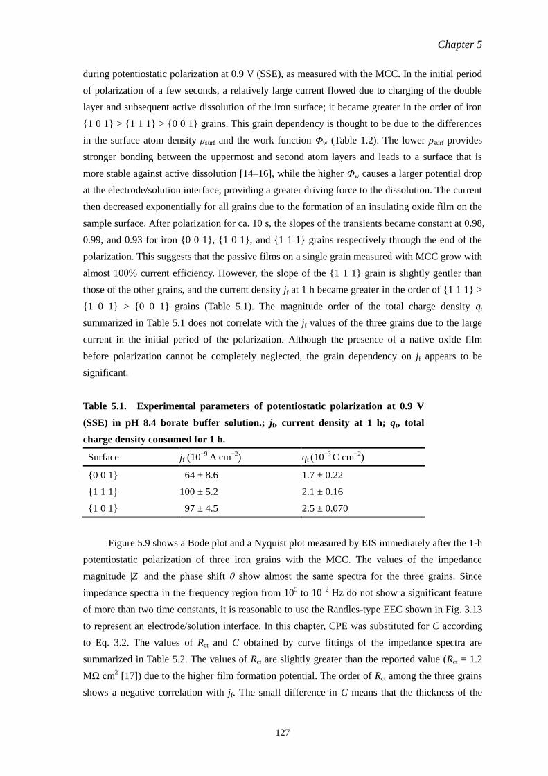
Chapter 5
127
during potentiostatic polarization at 0.9 V (SSE), as measured with the MCC. In the initial period
of polarization of a few seconds, a relatively large current flowed due to charging of the double
layer and subsequent active dissolution of the iron surface; it became greater in the order of iron
{1 0 1} > {1 1 1} > {0 0 1} grains. This grain dependency is thought to be due to the differences
in the surface atom density ρsurf and the work function Φw (Table 1.2). The lower ρsurf provides
stronger bonding between the uppermost and second atom layers and leads to a surface that is
more stable against active dissolution [14–16], while the higher Φw causes a larger potential drop
at the electrode/solution interface, providing a greater driving force to the dissolution. The current
then decreased exponentially for all grains due to the formation of an insulating oxide film on the
sample surface. After polarization for ca. 10 s, the slopes of the transients became constant at 0.98,
0.99, and 0.93 for iron {0 0 1}, {1 0 1}, and {1 1 1} grains respectively through the end of the
polarization. This suggests that the passive films on a single grain measured with MCC grow with
almost 100% current efficiency. However, the slope of the {1 1 1} grain is slightly gentler than
those of the other grains, and the current density jf at 1 h became greater in the order of {1 1 1} >
{1 0 1} > {0 0 1} grains (Table 5.1). The magnitude order of the total charge density qt
summarized in Table 5.1 does not correlate with the jf values of the three grains due to the large
current in the initial period of the polarization. Although the presence of a native oxide film
before polarization cannot be completely neglected, the grain dependency on jf appears to be
significant.
Table 5.1. Experimental parameters of potentiostatic polarization at 0.9 V
(SSE) in pH 8.4 borate buffer solution.; jf, current density at 1 h; qt, total
charge density consumed for 1 h.
Surface jf (10−9
A cm−2
) qt (10−3
C cm−2
)
{0 0 1} 64 ± 8.6 1.7 ± 0.22
{1 1 1} 100 ± 5.2 2.1 ± 0.16
{1 0 1} 97 ± 4.5 2.5 ± 0.070
Figure 5.9 shows a Bode plot and a Nyquist plot measured by EIS immediately after the 1-h
potentiostatic polarization of three iron grains with the MCC. The values of the impedance
magnitude |Z| and the phase shift θ show almost the same spectra for the three grains. Since
impedance spectra in the frequency region from 105 to 10
−2 Hz do not show a significant feature
of more than two time constants, it is reasonable to use the Randles-type EEC shown in Fig. 3.13
to represent an electrode/solution interface. In this chapter, CPE was substituted for C according
to Eq. 3.2. The values of Rct and C obtained by curve fittings of the impedance spectra are
summarized in Table 5.2. The values of Rct are slightly greater than the reported value (Rct = 1.2
MΩ cm2 [17]) due to the higher film formation potential. The order of Rct among the three grains
shows a negative correlation with jf. The small difference in C means that the thickness of the
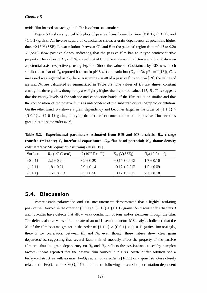
Chapter 5
128
oxide film formed on each grain differ less from one another.
Figure 5.10 shows typical MS plots of passive films formed on iron {0 0 1}, {1 0 1}, and
{1 1 1} grains. An inverse square of capacitance shows a grain dependency at potentials higher
than −0.15 V (SSE). Linear relations between C−2
and E in the potential region from −0.15 to 0.20
V (SSE) show positive slopes, indicating that the passive film has an n-type semiconductive
property. The values of Efb and ND are estimated from the slope and the intercept of the relation on
a potential axis, respectively, using Eq. 3.3. Since the value of C obtained by EIS was much
smaller than that of CH reported for iron in pH 8.4 borate solution (CH = 134 µF cm−2
[18]), C as
measured was regarded as CSC here. Assuming ε = 40 of a passive film on iron [19], the values of
Efb and ND are calculated as summarized in Table 5.2. The values of Efb are almost constant
among the three grains, though they are slightly higher than reported values [17,19]. This suggests
that the energy levels of the valence and conduction bands of the film are quite similar and that
the composition of the passive films is independent of the substrate crystallographic orientation.
On the other hand, ND shows a grain dependency and becomes larger in the order of {1 1 1} >
{0 0 1} > {1 0 1} grains, implying that the defect concentration of the passive film becomes
greater in the same order as ND.
Table 5.2. Experimental parameters estimated from EIS and MS analysis. Rct, charge
transfer resistance; C, interfacial capacitance; Efb, flat band potential; ND, donor density
calculated by MS equation assuming ε = 40 [19].
Surface Rct (106 Ω cm
2) C (10
−6 F cm
−2) Efb (V(SSE)) ND (10
20 cm
–3)
{0 0 1} 2.2 ± 0.24 6.2 ± 0.29 −0.17 ± 0.012 1.7 ± 0.10
{1 0 1} 1.8 ± 0.21 5.9 ± 0.14 −0.17 ± 0.013 1.5 ± 0.09
{1 1 1} 1.5 ± 0.054 6.3 ± 0.50 −0.17 ± 0.012 2.1 ± 0.18
5.4. Discussion
Potentiostatic polarization and EIS measurements demonstrated that a highly insulating
passive film formed in the order of {0 0 1} > {1 0 1} > {1 1 1} grains. As discussed in Chapters 3
and 4, oxides have defects that allow weak conduction of ions and/or electrons through the film.
The defects also serve as a donor state of an oxide semiconductor. MS analysis indicated that the
ND of the film became greater in the order of {1 1 1} > {0 0 1} > {1 0 1} grains. Interestingly,
there is no correlation between Rct and ND even though these values show clear grain
dependencies, suggesting that several factors simultaneously affect the property of the passive
film and that the grain dependency on Rct and ND reflects the passivation caused by complex
factors. It was reported that the passive film formed in pH 8.4 borate buffer solution had a
bi-layered structure with an inner Fe3O4 and an outer γ-Fe2O3 [10,11] or a spinel structure closely
related to Fe3O4 and γ-Fe2O3 [1,20]. In the following discussion, orientation-dependent
Chapter 5
129
passivation of iron is discussed based on the formation of a passive film with the bi-layered
structure.
In Chapters 3 and 4, the grain dependency in oxide formation was explained by the
difference of surface energy γ. Thus, it is also thought that γ (summarized in Table 1.2) is one
factor affecting grain-dependent passivation in pH 8.4 borate solution. Higher γ values mean
greater activity in the oxidation reaction at the substrate iron/oxide interface, even in an aqueous
solution environment. This implies that the growth rate of inner Fe3O4 is directly affected by γ.
The formation of Fe3O4 is thermodynamically feasible since ΔG for the formation of Fe3O4 from
Fe (and γ-Fe2O3) in Eq. 3.7 is negative (ΔG = −133.0 kJ mol−1
). Therefore, higher γ values can
lead to greater formation rates of Fe3O4 and make a thickness difference in the order of iron
{0 0 1} > {1 1 1} > {1 0 1} grains, which is the same as the order of γ in vacuum. The correlation
between γ and the thickness of an inner Fe3O4 layer was obtained for thermally grown oxides in
Chapter 4. However, it was difficult to observe the same relation in the thickness of oxide films
by 2D ellipsometry measurements during polarization in neutral solution. The small grain
dependency in the 2D ellipsometric images (Fig. 5.4) suggests that the difference in thickness
among substrate grain is significantly small and/or that the thickness resolution of the
ellipsometer is insufficient to optimize grain dependency. Since the dissolution of oxide film
and/or substrate through the oxide during anodic polarization is negligible in neutral aqueous
solution, it is thought that greater γ values indicate greater activity for the aging of the oxide film,
leading to the reduction of defects in the oxide rather than introducing Fe2+
ions into the oxide.
This means that Rct becomes greater in the order of {0 0 1} > {1 1 1} > {1 0 1} in pH 8.4 borate
solution. Although this order is slightly different from that of measured Rct and the difference in
Rct is less significant than what has been observed in sulfuric acid, it is thought that γ affected the
defect structure of the passive oxide film.
The anisotropic growth of oxides is another factor that develops a grain-dependent
passivation. It was reported in Chapter 4 that anisotropic growth affected the defect concentration
of oxides due to the compressive stress caused by the lateral component of the growth direction of
the oxides. The values of ND of thermally grown oxides became greater in the same order of the
magnitude of the lateral component. The same anisotropic relation between an oxide film and
substrate iron as the thermally grown oxide was also observed by Davenport et al. [1] for the
passive film formed on iron in pH 8.4 borate solution. They implied that the passive film formed
on the iron (0 0 1) face was less defective than the formed on the iron (1 0 1) plane, which is
related to the fact that the passive film on the iron {0 0 1} grain shows a higher Rct than on the
{1 0 1} grain. However, the implied defect structure does not explain the grain dependency of ND.
When the passive film formation is governed only by the movement of ions through the oxide
[22], Rct indicates the resistivity for ionic conduction in the oxide, whereas ND displays the density
of electron trap sites. Inconsistency in the grain dependency of Rct and ND suggests that ionic and
electronic conductions are in competition during the measurements of these parameters and in
Chapter 5
130
passive film formation, in which ionic conduction is a major factor during the passivation and
electronic conduction is dominant during the measurement of ND. It is thought that, here, ND
reflects the density of electron trap sites in the oxide film. The inverse magnitude order of {0 0 1}
and {1 0 1} for Rct to ND suggests that greater γ values reduce the lattice defects that act as
electron donors in the oxide film formed on {0 0 1} grains, compared to those formed on {1 0 1}
grains. The highest ionic conductivity and the largest ND on the iron {1 1 1} grain were caused by
both oxide formation with high γ, which is 95% of that on the iron {0 0 1} grain, and the
anisotropic growth of the oxide in the lateral direction.
Furthermore, the acidity of electrolyte solution could change the ratio of dissolution rate to
oxide formation rate, depending on the value of γ. In Chapter 3, the values of Rct of the passive
films formed in pH 1.3 sulfuric acid became greater in the order of {1 0 1} > {1 1 1} > {0 0 1}
grains. The current density during the potentiostatic polarization in pH 1.3 sulfuric acid is greater
than in pH 8.4 borate solution while the slope (−d log j / d log t) in pH 1.3 is gentler than in pH
8.4 solution. This is due to the dissolution of an oxide film and/or substrate iron through the film
into acidic media. It was reported in Chapter 3 that the consumption of γ-Fe2O3 for the formation
of Fe3O4 depended on γ. This conversion reaction would compete with the dissolution of γ-Fe2O3
into solution; the grain dependency of Rct would become much obvious in cases in which no
γ-Fe2O3 dissolves. In pH 8.4 borate buffer, where the dissolution reaction is negligibly small, the
difference in γ could be the main cause of differences in defect concentrations in the oxide. The
magnitude relation of Rct might be affected by differences in the formation rate and/or dissolution
rate of oxide, depending on both the γ of the substrate and the acidity of solution.
5.5. Conclusions
Grain-dependent passivation behavior of polycrystalline iron in pH 8.4 borate buffer was
investigated by means of in situ 2D ellipsometry and electrochemical measurements with the
MCC. Ellipsometric parameters changed on the entire sample surface as potentiostatic
polarization progressed. However, it was difficult to observe the clear heterogeneity of parameters,
depending on the metallographic texture of the substrate, even after polarization for 24 h. The
heterogeneity of a passive film thickness was too small to observe with the 2D ellipsometer
employed. Ex situ Raman spectroscopy and XPS analysis suggested that the composition of the
passive film was independent of the substrate crystallographic orientation. On the other hand,
micro-electrochemical measurements with the MCC demonstrated the grain dependency in the
charge transfer resistance Rct and the donor density ND of the passive film. Little correlation
between Rct and ND for the three iron grains indicated that the γ and anisotropic oxide growth
affect grain dependency during passivation. It was also suggested that the acidity of solution
during polarization affects anisotropic passive film formation, due to an increase in the dissolution
rate of the outer oxide layer.
Chapter 5
131
References
[1] A. J. Davenport, L. J. Oblonsky, M. P. Ryan, and M. F. Toney, J. Electrochem. Soc., 147,
2162 (2000).
[2] K. Fushimi, K. Azumi, and M. Seo, ISIJ Int., 39, 346 (1999).
[3] E. Desimoni, G. I. Casella, A. M. Salvi, T. R. I. Cataldi, and A. Morone, Carbon, 30, 527
(1992).
[4] G. T. Burstein and A. J. Davenport, J. Electrochem. Soc., 136, 936 (1989).
[5] N. Sato, K. Kudo, and R. Nishimura, J. Electrochem. Soc., 123, 1419 (1976).
[6] J. H. Weaver and H. P. R. Frederikse, in CRC Handbook of Chemistry and Physics, W. H.
Haynes and D. R. Lide, Editors, p. 12–126, CRC Press, New York (2011).
[7] N. Sato and K. Kudo, Electrochim. Acta, 16, 447 (1971).
[8] T. Ohtsuka, K. Kubo, and N. Sato, Corrosion, 42, 476 (1986).
[9] T. Ohtsuka, Mater. Trans., 37, 67 (1996).
[10] M. Nagayama and M. Cohen, J. Electrochem. Soc., 109, 781 (1962).
[11] M. P. Ryan, R. C. Newman, and G. E. Thompson, J. Electrochem. Soc., 142, L177 (1995).
[12] P. Keller and H.-H. Strehblow, Corros. Sci., 46, 1939 (2004).
[13] T. Nagatomi, S. Tanuma, and K. Goto, Surf. Interface Anal., 42, 1537 (2010).
[14] M. Seo and M. Chiba, Electrochim. Acta, 47, 319 (2001).
[15] M. Chiba and M. Seo, J. Electorchemical Soc., 150, B525 (2003).
[16] A. Schreiber, J. W. Schultze, M. M. Lohrengel, F. Kármán, and E. Kálmán, Electrochim.
Acta, 51, 2625 (2006).
[17] T. Yamamoto, K. Fushimi, S. Miura, and H. Konno, J. Electrochem. Soc., 157, C231 (2010).
[18] S. P. Harrington, F. Wang, and T. M. Devine, Electrochim. Acta, 55, 4092 (2010).
[19] K. Azumi, T. Ohtsuka, and N. Sato, J. Electrochem. Soc., 134, 1352 (1987).
[20] K. Kuroda, B. D. Cahan, G. Nazri, E. Yeager, and T. E. Mitchell, J. Electrochem. Soc., 129,
2163 (1982).
[21] W. E. Boggs, R. H. Kachik, and G. E. Pellissier, J. Electrochem. Soc., 112, 32 (1967).
[22] N. Sato, in Passivity of metals, R. P. Frankental and J. Kruger, Editors, p. 29, The
Electrochemical Society Inc., Princeton, NJ (1978).
[23] K. Iwauchi, Jpn. J. Appl. Phys., 10, 1520 (1971).
[24] K. S. Rane, A. K. Nikumbh, and A. J. Mukhedkar, J. Mater. Sci., 16, 2387 (1981).
[25] V. A. Hiremath and A. Venkataraman, Bull. Mater. Sci., 26, 391 (2003).
[26] G. V. Samsonov, The Oxide Handbook, p. 272, IFI/Plenum, New York (1973).
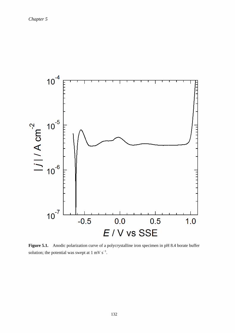
Chapter 5
132
Figure 5.1. Anodic polarization curve of a polycrystalline iron specimen in pH 8.4 borate buffer
solution; the potential was swept at 1 mV s−1
.
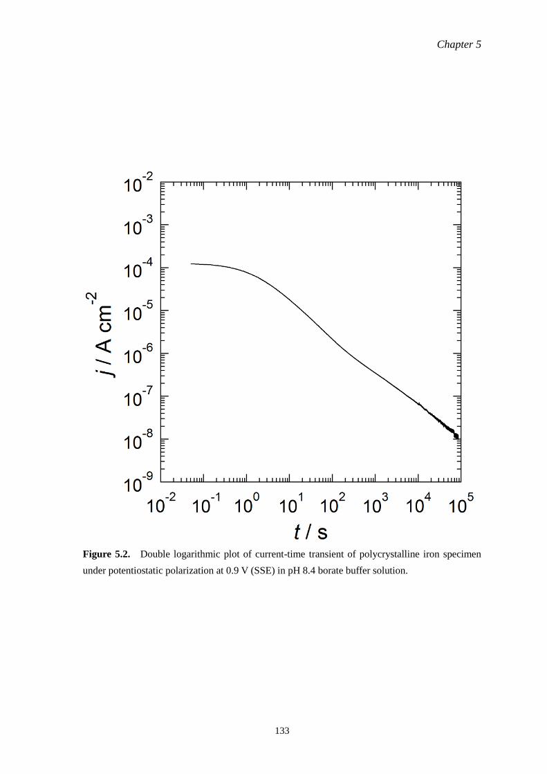
Chapter 5
133
Figure 5.2. Double logarithmic plot of current-time transient of polycrystalline iron specimen
under potentiostatic polarization at 0.9 V (SSE) in pH 8.4 borate buffer solution.
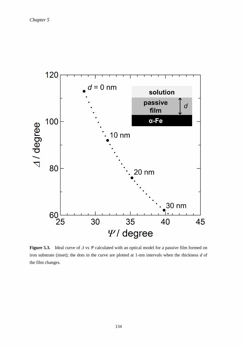
Chapter 5
134
Figure 5.3. Ideal curve of Δ vs Ψ calculated with an optical model for a passive film formed on
iron substrate (inset); the dots in the curve are plotted at 1-nm intervals when the thickness d of
the film changes.
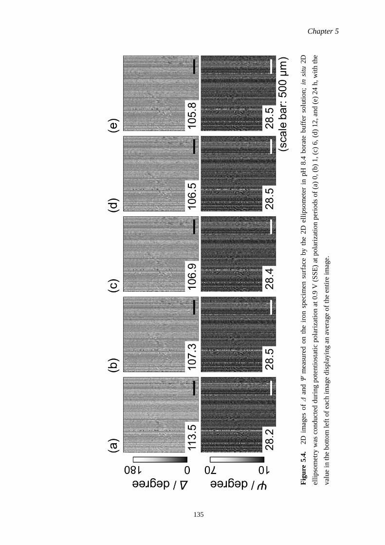
Chapter 5
135
Fig
ure
5.4
. 2
D i
mag
es o
f Δ
an
d Ψ
mea
sure
d o
n t
he
iron s
pec
imen
surf
ace
by t
he
2D
ell
ipso
met
er i
n p
H 8
.4 b
ora
te b
uff
er s
olu
tion
; in
sit
u 2
D
elli
pso
met
ry w
as c
on
du
cted
du
rin
g p
ote
nti
ost
atic
pola
riza
tion a
t 0.9
V (
SS
E)
at p
ola
riza
tion p
erio
ds
of
(a)
0,
(b)
1,
(c)
6,
(d)
12
, an
d (
e) 2
4 h
, w
ith
th
e
val
ue
in t
he
bo
tto
m l
eft
of
each
im
age
dis
pla
yin
g a
n a
ver
age
of
the
enti
re i
mag
e.
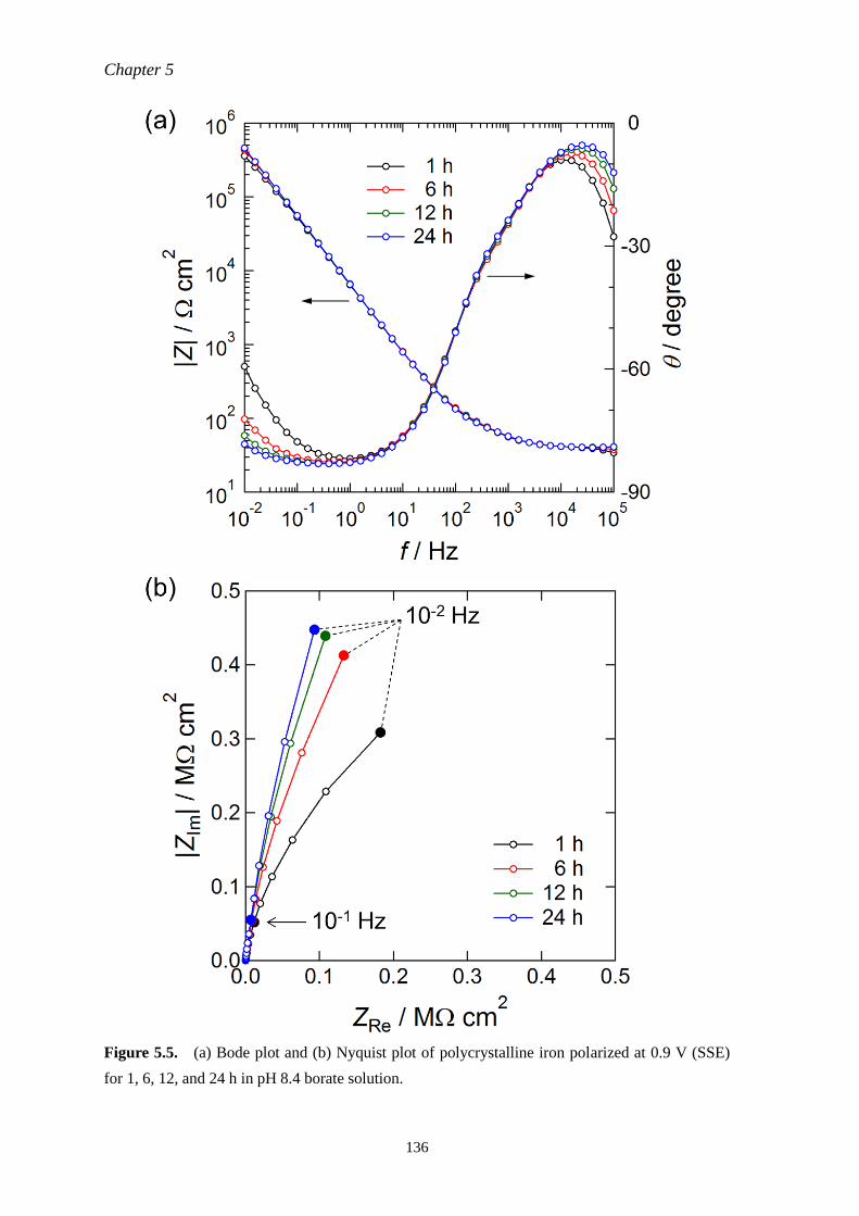
Chapter 5
136
Figure 5.5. (a) Bode plot and (b) Nyquist plot of polycrystalline iron polarized at 0.9 V (SSE)
for 1, 6, 12, and 24 h in pH 8.4 borate solution.
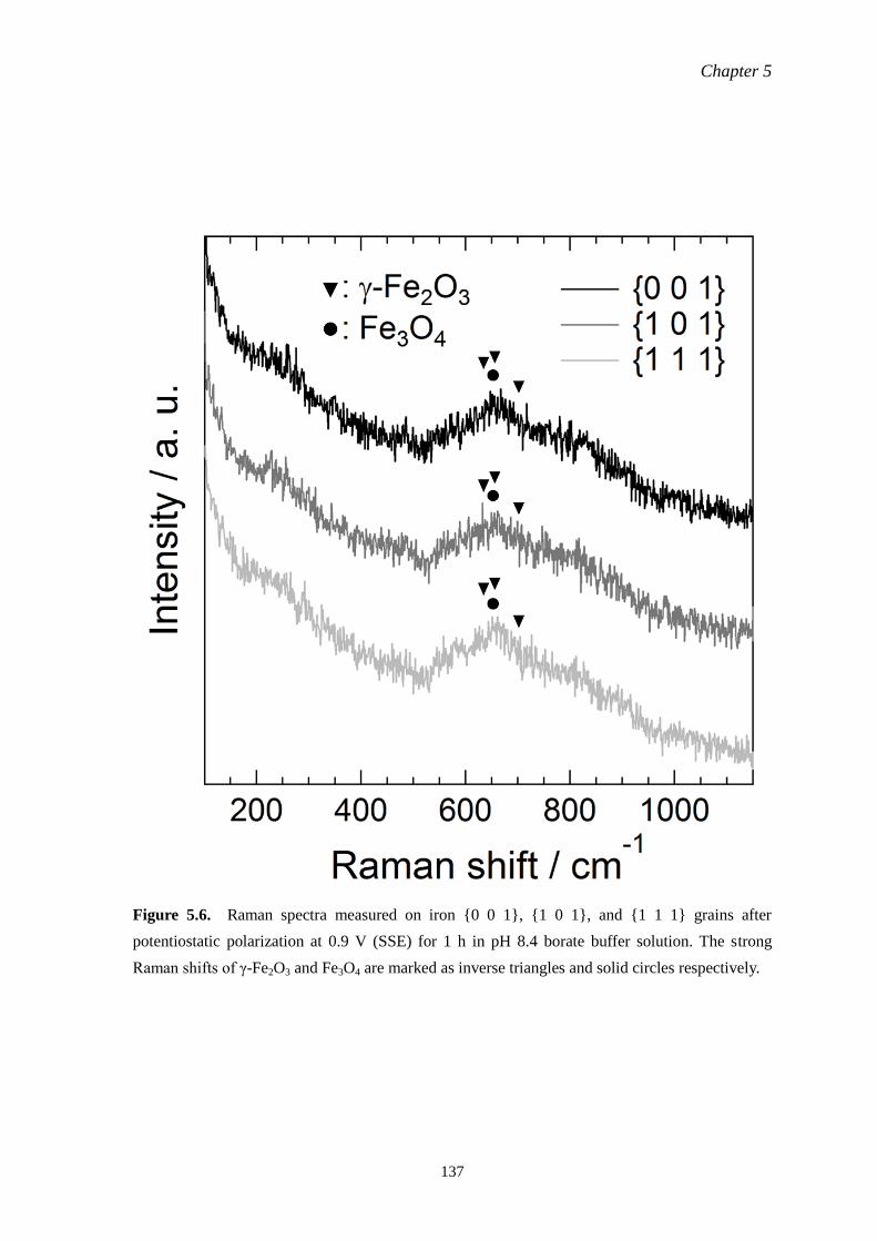
Chapter 5
137
Figure 5.6. Raman spectra measured on iron {0 0 1}, {1 0 1}, and {1 1 1} grains after
potentiostatic polarization at 0.9 V (SSE) for 1 h in pH 8.4 borate buffer solution. The strong
Raman shifts of γ-Fe2O3 and Fe3O4 are marked as inverse triangles and solid circles respectively.
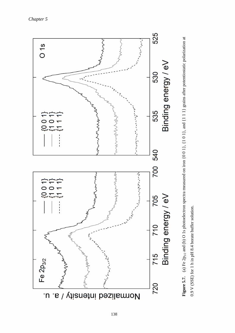
Chapter 5
138
Fig
ure
5.7
. (a
) F
e 2
p3/2 a
nd
(b
) O
1s
photo
elec
tron s
pec
tra
mea
sure
d o
n i
ron {
0 0
1},
{1 0
1}, an
d {
1 1
1} g
rain
s af
ter
po
ten
tio
stat
ic p
ola
riza
tio
n a
t
0.9
V (
SS
E)
for
1 h
in
pH
8.4
bo
rate
buff
er s
olu
tion.
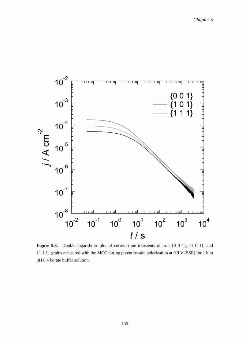
Chapter 5
139
Figure 5.8. Double logarithmic plot of current-time transients of iron {0 0 1}, {1 0 1}, and
{1 1 1} grains measured with the MCC during potentiostatic polarization at 0.9 V (SSE) for 1 h in
pH 8.4 borate buffer solution.
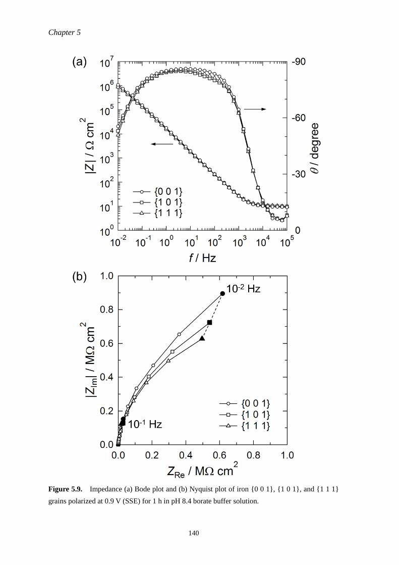
Chapter 5
140
Figure 5.9. Impedance (a) Bode plot and (b) Nyquist plot of iron {0 0 1}, {1 0 1}, and {1 1 1}
grains polarized at 0.9 V (SSE) for 1 h in pH 8.4 borate buffer solution.
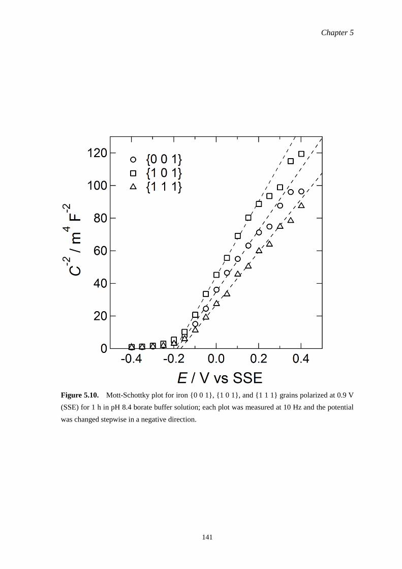
Chapter 5
141
Figure 5.10. Mott-Schottky plot for iron {0 0 1}, {1 0 1}, and {1 1 1} grains polarized at 0.9 V
(SSE) for 1 h in pH 8.4 borate buffer solution; each plot was measured at 10 Hz and the potential
was changed stepwise in a negative direction.
Chapter 6
142
Chapter 6
Summary
An oxide film formed on metallic materials plays an important role in preventing the
corrosion of metallic materials. The formation mechanism and characteristics of this oxide film
have been intensively studied since they directly affect the reliability and service time predictions
of metallic materials. Most metals and alloys used across a wide range of industries are
polycrystalline, and it has been pointed out that the formation rate, thickness, and characteristics
of the oxide film at the micro-region on a substrate depend on the metallographic structure, such
as the surface crystallographic orientation and grain boundaries. The detailed investigation of the
orientation-dependent oxidation behavior of polycrystalline metals and alloys was expected to
explain a detailed oxidation mechanism and the kinetics of practical metallic materials. Among
such materials, iron is the most commonly used metal in many industries as a base element of
steels; it is necessary for daily life. A clear understanding of the heterogeneity of the oxide film
formed on polycrystalline iron should lead to predicting the progress of corrosion on steels
accurately and to improving the reliability of service time estimations of steel-based structures.
Eventually, it could contribute to the realization of a genuinely sustainable society. On the other
hand, the technological advancements in the identification technique of surface crystallographic
orientations and in micro-electrochemical measurement methods have enabled precise analysis of
the oxidation behavior and the physicochemical property of an oxide film formed on a single
grain of a polycrystalline substrate. Grain-dependent oxidation behavior and the surface oxide
property of the single grain have been reported by several researchers, and the rough trends of the
grain-dependent oxidation are now becoming clear. However, the findings in previous reports
gave only fragmentary information on the way to the construction of a theory and the
development of an analytical technique to explain the relationship between oxide film formation
and corrosion resistance of metallic materials from the viewpoint of metallographic structure.
In this dissertation, an improved MCC method and in situ 2D ellipsometry were developed
as measurement techniques to investigate the heterogeneity of an oxide film formed on
polycrystalline iron. The passivation behavior of single grains and oxide film thickness and
degradation behavior of the entire polycrystalline surface were investigated using the developed
electrochemical measurement techniques.
In Chapter 1, the significance of studying corrosion and the grain-dependent corrosion of
polycrystalline metals were introduced. The motivation for investigating polycrystalline iron for
Chapter 6
143
this study and previous work on investigating corrosion behavior were both described. Finally, the
precise purpose of this dissertation was presented.
In Chapter 2, sample preparation, experimental setups, and procedures of the MCC and in
situ 2D ellipsometry were described.
In Chapter 3, passive films formed on single grains of a polycrystalline iron substrate were
investigated by the MCC in sulfuric acid. The current-time transients under potentiostatic
polarization depended heavily on the crystallographic orientation of the substrate surface.
Electrochemical impedance spectroscopy, XPS, and galvanostatic reduction revealed the grain
dependency in the charge transfer resistance Rct, composition, and the thickness of outer γ-Fe2O3
of the passive film. It was concluded that the grain dependency in the surface energy γ and
epitaxial relation between the oxide and substrate affected the defect structure of the passive film,
resulting in an inverse correlation between Rct and the thickness of γ-Fe2O3.
In Chapter 4, the heterogeneity of the thermally oxidized surface of a polycrystalline iron
substrate was investigated by means of 2D ellipsometry and the MCC. A bi-layered structure—an
inner Fe3O4 layer/an outer α-Fe2O3 layer—of the thermally grown oxide was confirmed by Raman
spectroscopy, SEM observation, and XPS. The oxide thickness evaluated by ex situ 2D
ellipsometry was summarized on an IPF of bcc iron as a contour map and the relationship
between the oxide thickness and surface crystallographic orientations was clarified.
Heterogeneous degradation behavior of the thermally oxidized surface was observed by in situ 2D
ellipsometry under galvanostatic polarization. The transients of ellipsometric parameters followed
different trajectories depending on the substrate orientation, indicating that an oxide film with
thicker inner Fe3O4 was more susceptible to the alteration of oxide properties caused by cathodic
currents. The donor density ND demonstrated by EIS measurements with the MCC showed a
positive correlation with dIL of the thickness of the inner Fe3O4 and γ of the iron substrate. It was
concluded that the anisotropic growth of two oxide layers affected dIL and the defect structure of
the outer α-Fe2O3 layer.
In Chapter 5, the passivation behavior of polycrystalline iron in pH 8.4 borate buffer
solution was investigated from the viewpoint of both a single grain and a whole polycrystalline
substrate. The growth of the passive film on a whole substrate was observed by in situ 2D
ellipsometry under potentiostatic polarization for 24 h. Ellipsometric images showed little grain
dependency in the passivation behavior, suggesting that the difference in thickness among
substrate grains was small and/or that the thickness resolution of the ellipsometer is insufficient to
optimize grain dependency. MCC measurements revealed the grain dependency in Rct and ND of
the passive film, but a clear correlation between these parameters was not observed. It was
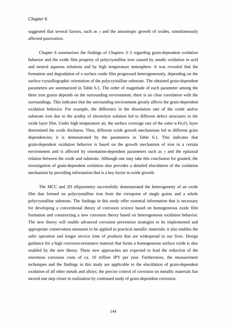
Chapter 6
144
suggested that several factors, such as γ and the anisotropic growth of oxides, simultaneously
affected passivation.
Chapter 6 summarizes the findings of Chapters 3–5 regarding grain-dependent oxidation
behavior and the oxide film property of polycrystalline iron caused by anodic oxidation in acid
and neutral aqueous solutions and by high temperature atmosphere. It was revealed that the
formation and degradation of a surface oxide film progressed heterogeneously, depending on the
surface crystallographic orientation of the polycrystalline substrate. The obtained grain-dependent
parameters are summarized in Table 6.1. The order of magnitude of each parameter among the
three iron grains depends on the surrounding environment; there is no clear correlation with the
surroundings. This indicates that the surrounding environment greatly affects the grain-dependent
oxidation behavior. For example, the difference in the dissolution rate of the oxide and/or
substrate iron due to the acidity of electrolyte solution led to different defect structures in the
oxide layer film. Under high temperature air, the surface coverage rate of the outer α-Fe2O3 layer
determined the oxide thickness. Thus, different oxide growth mechanisms led to different grain
dependencies; it is demonstrated by the parameters in Table 6.1. This indicates that
grain-dependent oxidation behavior is based on the growth mechanism of iron in a certain
environment and is affected by orientation-dependent parameters such as γ and the epitaxial
relation between the oxide and substrate. Although one may take this conclusion for granted, the
investigation of grain-dependent oxidation also provides a detailed elucidation of the oxidation
mechanism by providing information that is a key factor in oxide growth.
The MCC and 2D ellipsometry successfully demonstrated the heterogeneity of an oxide
film that formed on polycrystalline iron from the viewpoint of single grains and a whole
polycrystalline substrate. The findings in this study offer essential information that is necessary
for developing a conventional theory of corrosion science based on homogeneous oxide film
formation and constructing a new corrosion theory based on heterogeneous oxidation behavior.
The new theory will enable advanced corrosion prevention strategies to be implemented and
appropriate conservation measures to be applied to practical metallic materials; it also enables the
safer operation and longer service time of products that are widespread in our lives. Design
guidance for a high corrosion-resistance material that forms a homogeneous surface oxide is also
enabled by the new theory. These new approaches are expected to lead the reduction of the
enormous corrosion costs of ca. 10 trillion JPY per year. Furthermore, the measurement
techniques and the findings in this study are applicable to the elucidation of grain-dependent
oxidation of all other metals and alloys; the precise control of corrosion on metallic materials has
moved one step closer to realization by continued study of grain-dependent corrosion.
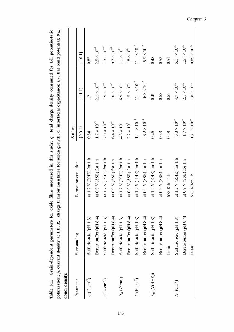
Chapter 6
145
Tab
le 6.1
. G
rain
-dep
end
ent
pa
ram
eter
s fo
r oxid
e fi
lms
mea
sure
d in
th
is st
ud
y;
qt, to
tal
cha
rge
den
sity
co
nsu
med
fo
r 1
-h p
ote
nti
ost
ati
c
pola
riza
tio
n;
j f,
curr
ent
den
sity
at
1 h
; R
ct, c
harg
e tr
an
sfer
res
ista
nce
for
oxid
e gro
wth
; C
, in
terf
aci
al
cap
aci
tan
ce;
Efb
, fl
at
ban
d p
ote
nti
al;
ND,
don
or
den
sity
.
{1
0 1
}
0.8
5
2.5
× 1
0−
3
1.3
× 1
0−
6
9.7
× 1
0−
8
1.1
× 1
05
1.8
× 1
06
11
× 1
0−
6
5
.9 ×
10
−6
0.4
8
0.5
3
0.5
1
5.1
×
10
20
1.5
×
10
20
0.8
9 ×
10
20
{1
1 1
}
1.2
2.1
× 1
0−
3
1.9
× 1
0−
6
1.0
× 1
0−
7
6.9
× 1
04
1.5
× 1
06
11
× 1
0−
6
6
.3 ×
10
−6
0.4
9
0.5
3
0.5
2
4.7
× 1
020
2.1
× 1
020
1.8
× 1
020
Surf
ace
{0 0
1}
0.5
4
1.7
× 1
0−
3
2.9
× 1
0−
6
6.4
× 1
0−
8
4.3
× 1
04
2.2
× 1
06
12
×
10
−6
6.2
× 1
0−
6
0.4
6
0.5
3
0.4
8
5.3
× 1
020
1.7
× 1
020
13
×
10
20
Form
atio
n c
ondit
ion
at 1
.2 V
(R
HE
) fo
r 1 h
at 0
.9 V
(S
SE
) fo
r 1 h
at 1
.2 V
(R
HE
) fo
r 1 h
at 0
.9 V
(S
SE
) fo
r 1 h
at 1
.2 V
(R
HE
) fo
r 1 h
at 0
.9 V
(S
SE
) fo
r 1 h
at 1
.2 V
(R
HE
) fo
r 1 h
at 0
.9 V
(S
SE
) fo
r 1 h
at 1
.2 V
(R
HE
) fo
r 1 h
at 0
.9 V
(S
SE
) fo
r 1 h
573 K
for
1 h
at 1
.2 V
(R
HE
) fo
r 1 h
at 0
.9 V
(S
SE
) fo
r 1 h
573 K
for
1 h
Su
rro
un
din
g
Su
lfuri
c ac
id (
pH
1.3
)
Bo
rate
bu
ffer
(pH
8.4
)
Su
lfuri
c ac
id (
pH
1.3
)
Bo
rate
bu
ffer
(pH
8.4
)
Su
lfuri
c ac
id (
pH
1.3
)
Bo
rate
bu
ffer
(pH
8.4
)
Su
lfuri
c ac
id (
pH
1.3
)
Bo
rate
bu
ffer
(pH
8.4
)
Su
lfuri
c ac
id (
pH
1.3
)
Bo
rate
bu
ffer
(pH
8.4
)
In a
ir
Su
lfuri
c ac
id (
pH
1.3
)
Bo
rate
bu
ffer
(pH
8.4
)
In a
ir
Par
amet
er
qt (C
cm
−2)
j f (
A c
m−
2)
Rct (
Ω c
m2)
C (
F c
m−
2)
Efb
(V
(RH
E))
ND
(cm
–3)
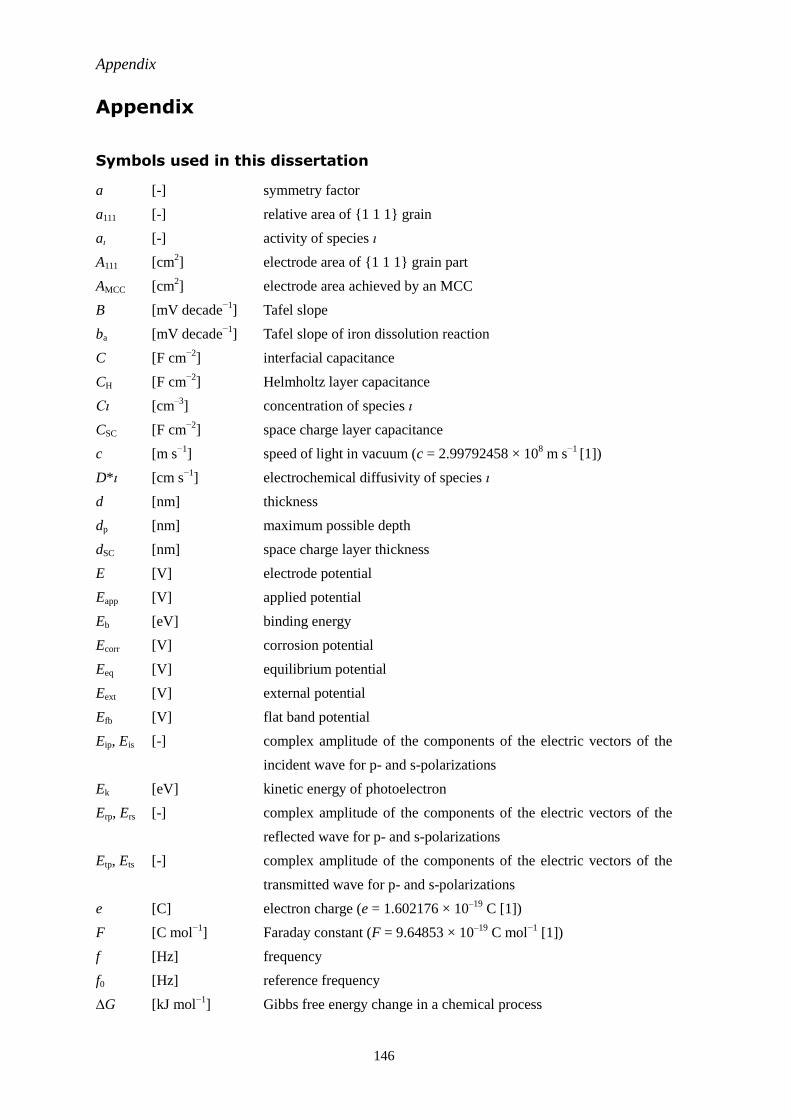
Appendix
146
Appendix
Symbols used in this dissertation
a [-] symmetry factor
a111 [-] relative area of {1 1 1} grain
aι [-] activity of species ι
A111 [cm2] electrode area of {1 1 1} grain part
AMCC [cm2] electrode area achieved by an MCC
B [mV decade−1
] Tafel slope
ba [mV decade−1
] Tafel slope of iron dissolution reaction
C [F cm−2
] interfacial capacitance
CH [F cm−2
] Helmholtz layer capacitance
Cι [cm–3
] concentration of species ι
CSC [F cm−2
] space charge layer capacitance
c [m s−1
] speed of light in vacuum (c = 2.99792458 × 10⁸ m s
−1 [1])
D*ι [cm s−1
] electrochemical diffusivity of species ι
d [nm] thickness
dp [nm] maximum possible depth
dSC [nm] space charge layer thickness
E [V] electrode potential
Eapp [V] applied potential
Eb [eV] binding energy
Ecorr [V] corrosion potential
Eeq [V] equilibrium potential
Eext [V] external potential
Efb [V] flat band potential
Eip, Eis [-] complex amplitude of the components of the electric vectors of the
incident wave for p- and s-polarizations
Ek [eV] kinetic energy of photoelectron
Erp, Ers [-] complex amplitude of the components of the electric vectors of the
reflected wave for p- and s-polarizations
Etp, Ets [-] complex amplitude of the components of the electric vectors of the
transmitted wave for p- and s-polarizations
e [C] electron charge (e = 1.602176 × 10⁻¹⁹
C [1])
F [C mol−1
] Faraday constant (F = 9.64853 × 10⁻¹⁹
C mol−1
[1])
f [Hz] frequency
f0 [Hz] reference frequency
∆G [kJ mol−1
] Gibbs free energy change in a chemical process
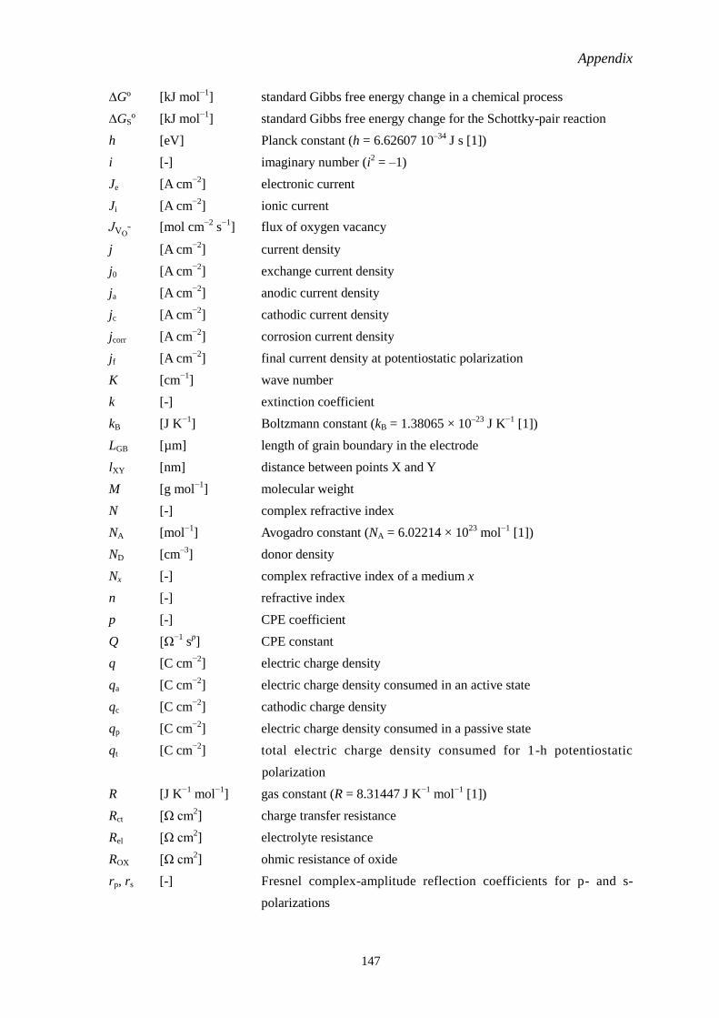
Appendix
147
∆Gº [kJ mol−1
] standard Gibbs free energy change in a chemical process
∆GSº [kJ mol−1
] standard Gibbs free energy change for the Schottky-pair reaction
h [eV] Planck constant (h = 6.62607 10–34
J s [1])
i [-] imaginary number (i2 = –1)
Je [A cm−2
] electronic current
Ji [A cm−2
] ionic current
JVO•• [mol cm
−2 s
−1] flux of oxygen vacancy
j [A cm−2
] current density
j0 [A cm−2
] exchange current density
ja [A cm−2
] anodic current density
jc [A cm−2
] cathodic current density
jcorr [A cm−2
] corrosion current density
jf [A cm−2
] final current density at potentiostatic polarization
K [cm−1
] wave number
k [-] extinction coefficient
kB [J K−1
] Boltzmann constant (kB = 1.38065 × 10⁻²³
J K−1
[1])
LGB [µm] length of grain boundary in the electrode
lXY [nm] distance between points X and Y
M [g mol−1
] molecular weight
N [-] complex refractive index
NA [mol−1
] Avogadro constant (NA = 6.02214 × 10²³
mol−1
[1])
ND [cm–3
] donor density
Nx [-] complex refractive index of a medium x
n [-] refractive index
p [-] CPE coefficient
Q [Ω−1
sp] CPE constant
q [C cm−2
] electric charge density
qa [C cm−2
] electric charge density consumed in an active state
qc [C cm−2
] cathodic charge density
qp [C cm−2
] electric charge density consumed in a passive state
qt [C cm−2
] total electric charge density consumed for 1-h potentiostatic
polarization
R [J K−1
mol−1
] gas constant (R = 8.31447 J K−1
mol−1
[1])
Rct [Ω cm2] charge transfer resistance
Rel [Ω cm2] electrolyte resistance
ROX [Ω cm2] ohmic resistance of oxide
rp, rs [-] Fresnel complex-amplitude reflection coefficients for p- and s-
polarizations
Appendix
148
s [m s−1
] speed of light in a medium
t [s] time
tp, ts [-] Fresnel complex-amplitude transmission coefficients for p- and s-
polarizations
tpa [s] passivating time
u [cm s−1
] velocity of drift of ions in an oxide film
T [K] absolute temperature
V [V] voltage drop across thin oxide film
X [cm] oxide film thickness at t
X1 [cm] characteristic distance depending on the interfacial potential
difference and temperature
XL [cm] limiting film thickness
|Z| [Ω cm2] impedance magnitude
ZIm [Ω cm2] imaginary part of impedance
ZRe [Ω cm2] real part of impedance
z [-] valence
α [-] coefficient for the potential dependence of ∆ϕf/s
αa [cm−1
] absorption coefficient
αp [-] phase change
β [-] coefficient for the pH dependence of ∆ϕf/s
βp [-] film phase thickness (βp = αp/2)
γ [J m−1
] surface energy
Δ [degrees] differential change in phase between vibrations of p- and s-
polarizations
δrp, δrs [degrees] arguments of rp and rs
ε [-] dielectric constant
ε0 [J−1
C2 m
−1] permittivity in vacuum (ε0 = 8.85419 × 10
–12 J
−1 C
2 m
−1 [1])
εF [V cm−1
] field strength
η [V] overpotential
θ [degrees] phase shift
θ0 [degrees] incident angle
θ1 [degrees] refraction angle
λ [nm] wavelength of light
μι [kJ mol−1
] chemical potential of species ι
ν [s−1
] frequency of electromagnetic wave
Ρ [-] ratio of the complex Fresnel reflection coefficients for p- and s-
polarizations
ρ [Ω m] electrical resistivity
Appendix
149
ρox [g cm–3
] density of oxide
ρsurf [cm–2
] surface atom density
σ [Ω–1
m–1
] electrical conductivity
Φ [degrees] Euler angle between the Z axis and the z axis
Φw [eV] work function
φ1 [degrees] Euler angle between the X axis and the NSC axis
φ2 [degrees] Euler angle between the NSC axis and the x axis
∆ϕf [V] potential drop across the oxide film on a metal
∆ϕR
[V] potential drop at a solution/reference electrode interface
∆ϕf/s
[V] potential drop at a film/solution interface
∆ϕm/f
[V] potential drop at a metal/film interface
Ψ [degrees] differential change in amplitude between vibrations of p- and s-
polarizations
ω”m [Hz] frequency at which the |ZIm| shows a maximum value
Ω [cm3 mol
−1] molecular volume
[1] P. W. Atkins and J. De Paula, Atkins’ Physical Chemistry, 10 th Ed., Oxford University Press,
Oxford (2014).
Abbreviations
AES Auger electron spectroscopy
bcc body-centered cubic
BE backscattered electron
CP cross section polisher
CPE constant phase element
DFT density functional theory
EBSD electron backscatter diffraction
EES equivalent electronic circuit
EIS electrochemical impedance spectroscopy
ESCA electron spectroscopy for chemical analysis
FIB focused ion beam
GNP gross national product
IDR iron dissolution reaction
IPF inverse pole figure
MCC micro-capillary cell
MS Mott-Schottky
ND normal direction
Appendix
150
OCP open circuit potential
PCA photonic crystal array
RD rolling direction
rds rate-determining step
RHE reversible hydrogen electrode
TD transverse direction
SE secondary electron
SECM scanning electrochemical microscopy
SEM scanning electron microscope
SERS surface-enhanced Raman spectroscopy
SIMS secondary ion mass spectroscopy
SHE standard hydrogen electrode
SSE silver-silver chloride electrode
STM scanning tunneling microscopy
TEM transmission electron microscopy
XANES X-ray absorption near edge structure
XPS X-ray photoelectron spectroscopy
XRD X-ray diffraction
List of publications
151
List of publications
[1] Yu Takabatake, Koji Fushimi, Takayuki Nakanishi, and Yasuchika Hasegawa,
“Grain-Dependent Passivation of Iron in Sulfuric Acid Solution”, Journal of The
Electrochemical Society, Vol. 161, Issue 14, pp. C594–C600 (2014).
[2] Yu Takabatake, Yuichi Kitagawa, Takayuki Nakanishi, Yasuchika Hasegawa, and Koji
Fushimi, “Heterogeneity of a Thermal Oxide Film Formed on Polycrystalline Iron Observed
by Two-Dimensional Ellipsometry”, Journal of The Electrochemical Society, Vol. 163, Issue
14, pp. C815–C822 (2016).
Other publications
[1] Koji Fushimi, Yu Takabatake, Takayuki Nakanishi, and Yasuchika Hasegawa,
“Microelectrode techniques for corrosion research of iron”, Electrochimica Acta, Vol. 113, pp.
741–747 (2013).
[2] Hisataka Kataoka, Takayuki Nakanishi, Shun Omagari, Yu Takabatake, Yuichi Kitagawa, and
Yasuchika Hasegawa, “Drastically Improved Durability and Efficiency of Silicon Solar Cells
Using Hyper-Stable Lanthanide Coordination Polymer Beads”, Bulletin of the Chemical
Society of Japan, Vol. 89, Issue 1, pp. 103–109 (2016).
Acknowledgements
152
Acknowledgements
I would like to express my deepest gratitude to my supervisor Associate professor
Koji Fushimi for the continuous support and encouragement throughout my Ph. D.
program, for his kind guidance and immense knowledge.
I would like to show my sincere appreciation to Professor Kazuhisa Azumi, Kei
Murakoshi, Hiroki Habazaki, and Yasuchika Hasegawa for being my advisors and giving
insightful comments and suggestions to develop my research.
I also would like to thank Associate professor Masatoshi Sakairi, Assistant
professor Takayuki Nakanishi and Yuichi Kitagawa for their helpful advice and warm
encouragement.
My sincere thanks also go to colleagues in the laboratory of Advanced Materials
Chemistry (AMC), Graduate School of Chemical Sciences and Engineering, Hokkaido
University, Japan, who had helped my daily work.
Finally, I gratefully acknowledge the financial support from the Japan Society for
the Promotion of Science (JSPS) for Young Scientists by a Grant-in-Aid for JSPS Fellows
(No. 26000231).
Yu Takabatake
Sapporo, Japan
March 2017