study on the converted total least squares method and its
TRANSCRIPT
Universität Stuttgart
Geodätisches Institut
Study on the Converted Total Least Squaresmethod and its application in coordinate
transformation
Bachelorarbeit im Studiengang
Geodäsie und Geoinformatik
an der Universität Stuttgart
Dalu Dong
Stuttgart, April 2017
Betreuer: Prof. Dr.-Ing. Nico SneeuwUniversität Stuttgart
Dr.-Ing. Jianqing CaiUniversität Stuttgart

II

Erklärung der Urheberschaft
Ich erkläre hiermit an Eides statt, dass ich die vorliegende Arbeit ohne Hilfe Dritter und ohneBenutzung anderer als der angegebenen Hilfsmittel angefertigt habe; die aus fremden Quellendirekt oder indirekt übernommenen Gedanken sind als solche kenntlich gemacht. Die Arbeitwurde bisher in gleicher oder ähnlicher Form in keiner anderen Prüfungsbehörde vorgelegtund auch noch nicht veröffentlicht.
Ort, Datum Unterschrift
III

Abstract
This Thesis gives a brief introduction to Total Least Squares (TLS) comparing with the classicalLS, and its common solutions by singular value decomposition (SVD) approaches and the it-eration, also following with the advantages and disadvantages of both methods. One methodnamed Converted Total Least Squares (CTLS) dealing with the errors-in-variables (EIV) modelcan solve the problems of both. The basic idea of it is to take the stochastic design matrix el-ements as virtual observations, and the TLS problem can be transformed into a LS problem.The significance of CTLS lies not merely in attaining the optimal estimation of parameters andmore importantly in completing the theory of TLS with classical LS. As a comparison, anotherestimation method based on Partial-EIV model will also be presented, which can deal with theTLS problems with iterative algorithm. The coordinate transformation parameter estimationformula of both algorithms are derived. By specifying the accuracy assessment formulas ofCTLS, this thesis identifies rigorously the degree of freedom of the EIV model in theory andsolves the bottleneck problem of TLS that restricts the application and development of TLS.
Key words Total Least Squares, singular value decomposition, errors-in-variables, virtual ob-servation, Partial-EIV model, accuracy assessment.
V

VI

VII
Contents
1 Introduction 1
2 Transformation models and data preparation 32.1 6-parameter affine transformation models(2D) . . . . . . . . . . . . . . . . . . . . 32.2 7-parameter Helmert transformation models(3D) . . . . . . . . . . . . . . . . . . . 42.3 Data preparation and the analysis with collocated points in Baden-Württemberg 5
3 Total Least Squares 83.1 Introduction . . . . . . . . . . . . . . . . . . . . . . . . . . . . . . . . . . . . . . . . 83.2 Total Least Squares with singular value decomposition(SVD) . . . . . . . . . . . . 103.3 Total Least Squares with the Euler-Lagrange approach . . . . . . . . . . . . . . . . 113.4 Total Least Squares based on Partial-EIV model . . . . . . . . . . . . . . . . . . . . 13
4 Converted Total Leat Squares 164.1 Introduction and mathematical foundation . . . . . . . . . . . . . . . . . . . . . . 164.2 Estimation formula of unit weight variance . . . . . . . . . . . . . . . . . . . . . . 184.3 Co-factor matrix of parameters . . . . . . . . . . . . . . . . . . . . . . . . . . . . . 19
5 Application of the coordinate transformation in Baden-Württenberg with differentEstimation methods 205.1 Transformation in two-dimensional(2D) . . . . . . . . . . . . . . . . . . . . . . . . 20
5.1.1 Transformation with Total Least Squares(SVD) . . . . . . . . . . . . . . . . 215.1.2 Transformation with Total Least Squares based on Partial-EIV model . . . 225.1.3 Transformation with Converted Total Least Squares . . . . . . . . . . . . . 235.1.4 Presentation and Comparison of the results . . . . . . . . . . . . . . . . . . 24
5.2 Transformation in three-dimensional(3D) . . . . . . . . . . . . . . . . . . . . . . . 285.2.1 Transformation with Total Least Squares(SVD) . . . . . . . . . . . . . . . . 295.2.2 Transformation with Total Least Squares based on Partial-EIV model . . . 305.2.3 Transformation with Converted Total Least Squares . . . . . . . . . . . . . 325.2.4 Presentation and Comparison of the results . . . . . . . . . . . . . . . . . . 33
6 Conclusion 39
VIII
List of Figures
2.1 Horizontal residuals after 6-parameter affine transformation in Baden-Württemberg network . . . . . . . . . . . . . . . . . . . . . . . . . . . . . . . . . . 6
2.2 Horizontal residuals after 7-parameter Helmert transformation in Baden-Württemberg network . . . . . . . . . . . . . . . . . . . . . . . . . . . . . . . . . . 7
4.1 Illustrate the basic idea of the algorithm . . . . . . . . . . . . . . . . . . . . . . . . 17
5.1 Illustrate the process for 6p-affine transformation . . . . . . . . . . . . . . . . . . 215.2 Horizontal residuals after 6-parameter affine transformation in Baden-
Württemberg network . . . . . . . . . . . . . . . . . . . . . . . . . . . . . . . . . . 265.3 Horizontal residuals after 6-parameter affine transformation in Baden-
Württemberg network . . . . . . . . . . . . . . . . . . . . . . . . . . . . . . . . . . 265.4 Horizontal residuals after 6-parameter affine transformation in Baden-
Württemberg network . . . . . . . . . . . . . . . . . . . . . . . . . . . . . . . . . . 275.5 Horizontal residuals after 6-parameter affine transformation in Baden-
Württemberg network . . . . . . . . . . . . . . . . . . . . . . . . . . . . . . . . . . 275.6 Illustrate the process for 7p-Helmert transformation . . . . . . . . . . . . . . . . . 295.7 Horizontal residuals after 7-parameter Helmert transformation in Baden-
Württemberg network . . . . . . . . . . . . . . . . . . . . . . . . . . . . . . . . . . 355.8 Horizontal residuals after 7-parameter Helmert transformation in Baden-
Württemberg network . . . . . . . . . . . . . . . . . . . . . . . . . . . . . . . . . . 355.9 Horizontal residuals after 7-parameter Helmert transformation in Baden-
Württemberg network . . . . . . . . . . . . . . . . . . . . . . . . . . . . . . . . . . 365.10 Horizontal residuals after 7-parameter Helmert transformation in Baden-
Württemberg network . . . . . . . . . . . . . . . . . . . . . . . . . . . . . . . . . . 36

IX
List of Tables
2.1 Transformation parameters and their standard deviation with 131 BWREF points 6
5.1 Comparison of 6-parameter affine transformation parameters with 4 estimators . 255.2 Numerical deviation of 6-parameter affine transformation with 4 estimators . . . 255.3 Comparison of 7-parameter Helmert transformation parameters with 4 estimators 345.4 Numerical deviation of 7-parameter Helmert transformation with 4 estimators . 345.5 First 10 rows of the residuals by design matrix with 2D affine transformation . . 385.6 First 10 rows of the residuals by design matrix with 3D Helmert transformation . 38
1
Chapter 1
Introduction
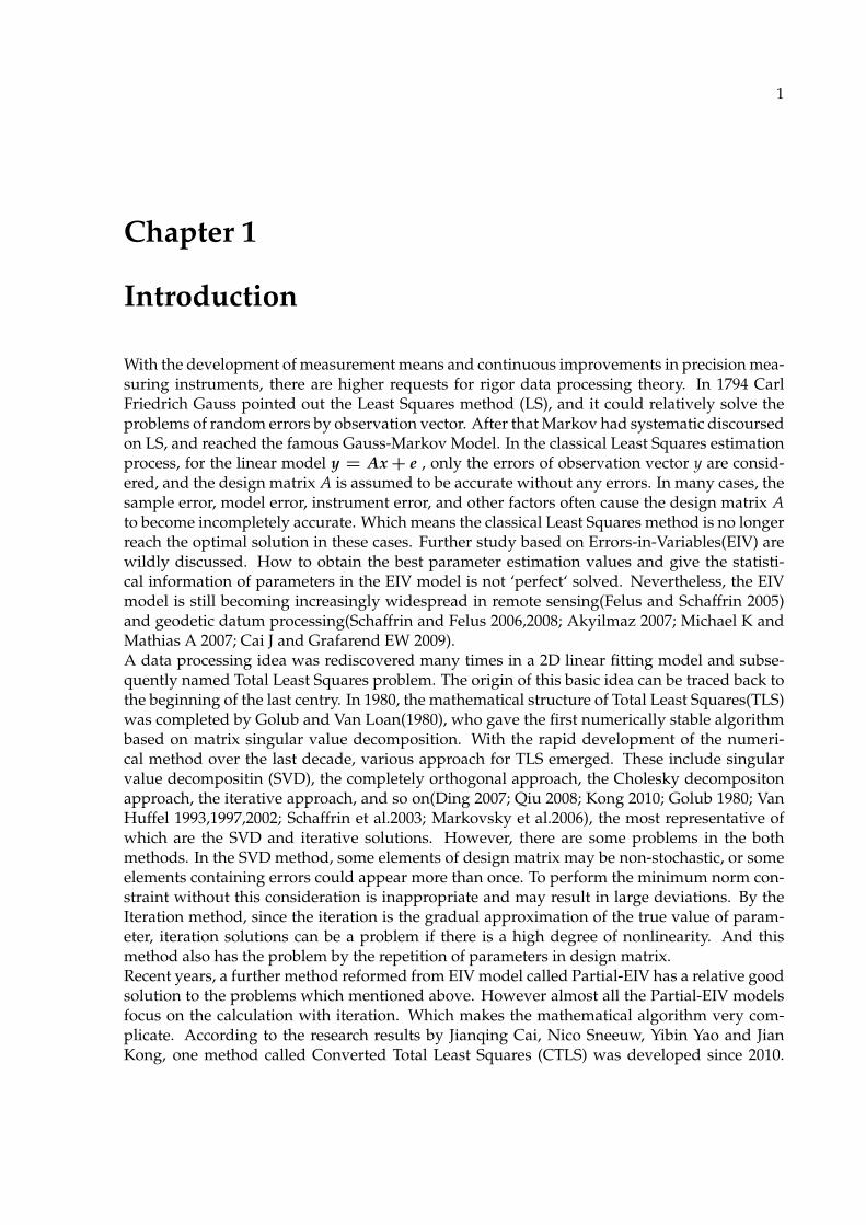
With the development of measurement means and continuous improvements in precision mea-suring instruments, there are higher requests for rigor data processing theory. In 1794 CarlFriedrich Gauss pointed out the Least Squares method (LS), and it could relatively solve theproblems of random errors by observation vector. After that Markov had systematic discoursedon LS, and reached the famous Gauss-Markov Model. In the classical Least Squares estimationprocess, for the linear model y = Ax + e , only the errors of observation vector y are consid-ered, and the design matrix A is assumed to be accurate without any errors. In many cases, thesample error, model error, instrument error, and other factors often cause the design matrix Ato become incompletely accurate. Which means the classical Least Squares method is no longerreach the optimal solution in these cases. Further study based on Errors-in-Variables(EIV) arewildly discussed. How to obtain the best parameter estimation values and give the statisti-cal information of parameters in the EIV model is not ‘perfect‘ solved. Nevertheless, the EIVmodel is still becoming increasingly widespread in remote sensing(Felus and Schaffrin 2005)and geodetic datum processing(Schaffrin and Felus 2006,2008; Akyilmaz 2007; Michael K andMathias A 2007; Cai J and Grafarend EW 2009).A data processing idea was rediscovered many times in a 2D linear fitting model and subse-quently named Total Least Squares problem. The origin of this basic idea can be traced back tothe beginning of the last centry. In 1980, the mathematical structure of Total Least Squares(TLS)was completed by Golub and Van Loan(1980), who gave the first numerically stable algorithmbased on matrix singular value decomposition. With the rapid development of the numeri-cal method over the last decade, various approach for TLS emerged. These include singularvalue decompositin (SVD), the completely orthogonal approach, the Cholesky decompositonapproach, the iterative approach, and so on(Ding 2007; Qiu 2008; Kong 2010; Golub 1980; VanHuffel 1993,1997,2002; Schaffrin et al.2003; Markovsky et al.2006), the most representative ofwhich are the SVD and iterative solutions. However, there are some problems in the bothmethods. In the SVD method, some elements of design matrix may be non-stochastic, or someelements containing errors could appear more than once. To perform the minimum norm con-straint without this consideration is inappropriate and may result in large deviations. By theIteration method, since the iteration is the gradual approximation of the true value of param-eter, iteration solutions can be a problem if there is a high degree of nonlinearity. And thismethod also has the problem by the repetition of parameters in design matrix.Recent years, a further method reformed from EIV model called Partial-EIV has a relative goodsolution to the problems which mentioned above. However almost all the Partial-EIV modelsfocus on the calculation with iteration. Which makes the mathematical algorithm very com-plicate. According to the research results by Jianqing Cai, Nico Sneeuw, Yibin Yao and JianKong, one method called Converted Total Least Squares (CTLS) was developed since 2010.

Chapter 1 Introduction 2
This method has been culculated without iteration and at the same time solve the problem bythe repetition of elements and the non-stochastic elements containing errors in design matrix.In this thesis the two transformation models (6-parameter affine transformation model and 7-parameter Helmert transformation model) are firstly reviewed. They will be analyzed by using131 BWREF points in Baden-Württemberg. Then the mathematic foundation of TLS method isreviewed. Two different solutions SVD (Van Huffel, 1991) and iteration approach (Schaffrin,2005) and the Partial-EIV model are introduced. And the representative experiments will beimplemented through the coordinate transformation in Baden-Württemberg. As a compari-son, the transformation parameters estimated by LS, TLS (SVD), Partial-EIV model and CTLSwill be represented and discussed.
3
Chapter 2
Transformation models and data preparation
2.1 6-parameter affine transformation models(2D)
In the case of map coordinates, which result from the projection of the reference ellipsoid intoplane, a two-dimensional model is more useful. For example, when between the respectivereference systems (DHDN, Bessel and ETRS89, GRS80) no direct mathematical relationshipexists. Two-dimensional transformation models are used. As a result, the Gauss-Krügercoordinates of the net points in DHDN can be transformed only over collocated pointsinto UTM coordinates related to ETR89. For the two dimensional transformation models,there are three , four, five, or six transformation parameters, whose number depends on therespective requirements. Because the models with three or five parameters can make for someproblems, e.g. non-linear equations problem, so they will not be considered here. In mostapplications of the plane-transformation, the 6-parameter affine transformation model is usedand is recommended by the Surveying Authorities of the States of the Federal Republic ofGermany. Therefor, the 6-parameter affine model will be reviewed and applied in estimatingthe parameters of the plane transformation parameters based on 131 collocated points inBaden-Württemberg(Cai, 2006).
With the planar affine transformation, where six parameters are to be determined, bothcoordinate directions are rotated with two different angles α and β. So that not only thedistances and the angles are distorted, but usually also the original orthogonality of the axesof coordinates is lost. An affine transformation preserves collinearity and ratios of distances.While an affine transformation preserves proportions on lines, it does not necessarily preserveangles or lengths(Cai, 2006).
The 6-parameter affine transformation model between any two plane coordinates systems, e.g.from Grauss-Krüger coordinate(H,R) in DHDN (G) directly to the UTM-Coordinate (N,E) inETRS89 can be written as [
NE
]=
[λHcosα −λRsinβλHsinα λRcosβ
] [HR
]+
[tNtE
](2.1)
Where tN and tE are translation parameters; α and β are rotation parameters; λH and λR arescale corrections.

Chapter 2 Transformation models and data preparation 4
2.2 7-parameter Helmert transformation models(3D)
In most applications of three-dimensional transformation three seven parameter similaritytransformation 3D Helmert model, also called after Bursa-Wolf (Bursa 1962, Wolf 1963),Molodensky-Badekas (Molodensky et al., 1960; Badekas, 1969) and Veis(1960) models aredeveloped and used. Though the three seven parameter models are expressed in differentforms with different origin and parameters, their transformation results are completelyequialent. The description and the application of the Molodensky-Badekas models are referredto Heck(1995) and Ihde et al.(1995).
• Bursa-Wolf model XGYGZG
= (1 + dλ)
1 γ −β−γ 1 αβ −α 1
XLYLZL
+
TXTYTZ
(2.2)
•Molodensky-Badekas modelXGYGZG
=
XLYLZL
+
TXTYTZ
+
0 ω −ψ−ω 0 εψ −ε 0
XL − XL0YL − YL0ZL − ZL0
+ dλ
XL − XL0YL − YL0ZL − ZL0
(2.3)
• Veis modelXGYGZG
=
XLYLZL
+
TXTYTZ
+ dλ
XL − XL0YL − YL0ZL − ZL0
+
0 ZL0 − ZL YL − YL0ZL − ZL0 0 XL0 − XLYL0 − YL XL − XL0 0
−sinBL0cosLL0 −sinLL0 cosBL0cosLL0−sinBL0sinLL0 cosLL0 cosBL0sinLL0
cosBL0 0 sinBL0
ωxωyωz
(2.4)
The similarity of the transformation is particularly important since the conformal characteristicof the coordinates after the transformation are maintained. They are applied particular forthe discrepancies between a local (e.g. DHDN related Bessel ellipsoid) and a global referencesystem(e.g. ETRS89 related GRS80 Ellipsoid) which are due to the differences in the geodeticdatum. However, the three seven parameter models are expressed in different forms withdifferent origin and parameters, their transformation results are completely equivalent. So7-parameter Helmert model is used most commonly(Cai, 2006).
The further reasons for the choice of 7-parameter Helmert transformation model are:
• It is the only known method which allows a direct interpretation of origin shifts.
• The rotations around the ’Earth-Centered, Earth-Fixed(ECEF)’ Cartesian axes can havephysical interpretations in global reference frames.
• It perform a conformal transformation, where the ratios of distances and the angles pre-serve invariantly.(Cai, 2006)
Chapter 2 Transformation models and data preparation 5
It performs a conformal transformation, where the ratios of distances and the angles preserveinvariantly. A ’local’ non-geocentric XL,YL,ZL-system can be transformed into a ’global’geocentric XG,YG,ZG-system with the help of a 7-parameter Helmert transformation model.XG
YGZG
=
TXTYTZ
+ (1 + dλ)
1 γ −β−γ 1 αβ −α 1
XLYLZL
∼=
TXTYTZ
+
dλ γ −β−γ dλ αβ −α dλ
XLYLZL
+
XLYLZL
(2.5)
Where TX,TY,TZ are translate parameters; α , β and γ are differential rotation parameters; dλ isscale correction.
2.3 Data preparation and the analysis with collocated points inBaden-Württemberg
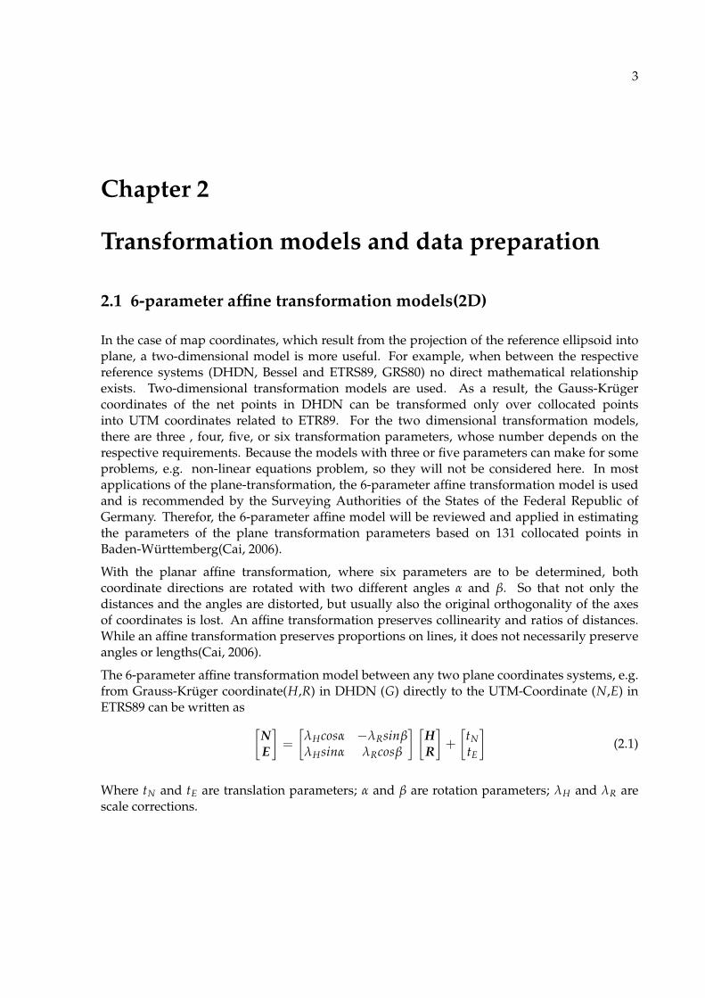
In preparation of local coordinate of collocated points the Gauss-Krüger coordinates of DHDNwill be transformed to Bessel ellipsoidal coordinates latitude (BL) and longitude (LL) throughinverse conformal mapping formulas and the conversion of ellipsoidal coordinates (BL,LL,HL)to geodetic Cartesian coordinates (XL,YL,ZL) and the reverse conversion are accomplishedthrough the general formula. For the global coordinates can be also converted with the samealgorithms on the GRS80 ellipsoid. Then we can construct the quasi-observations with the 131collocated points (131 BWREF points in Baden-Württemberg) and perform the estimation ofthe transformation parameters of the 7-parameter Helmert transformation and the 6-parameteraffine transformation. The transformation parameter solutions using above two models arelisted in table I and the residuals are illustrated in figure 2.1 and figure 2.2.
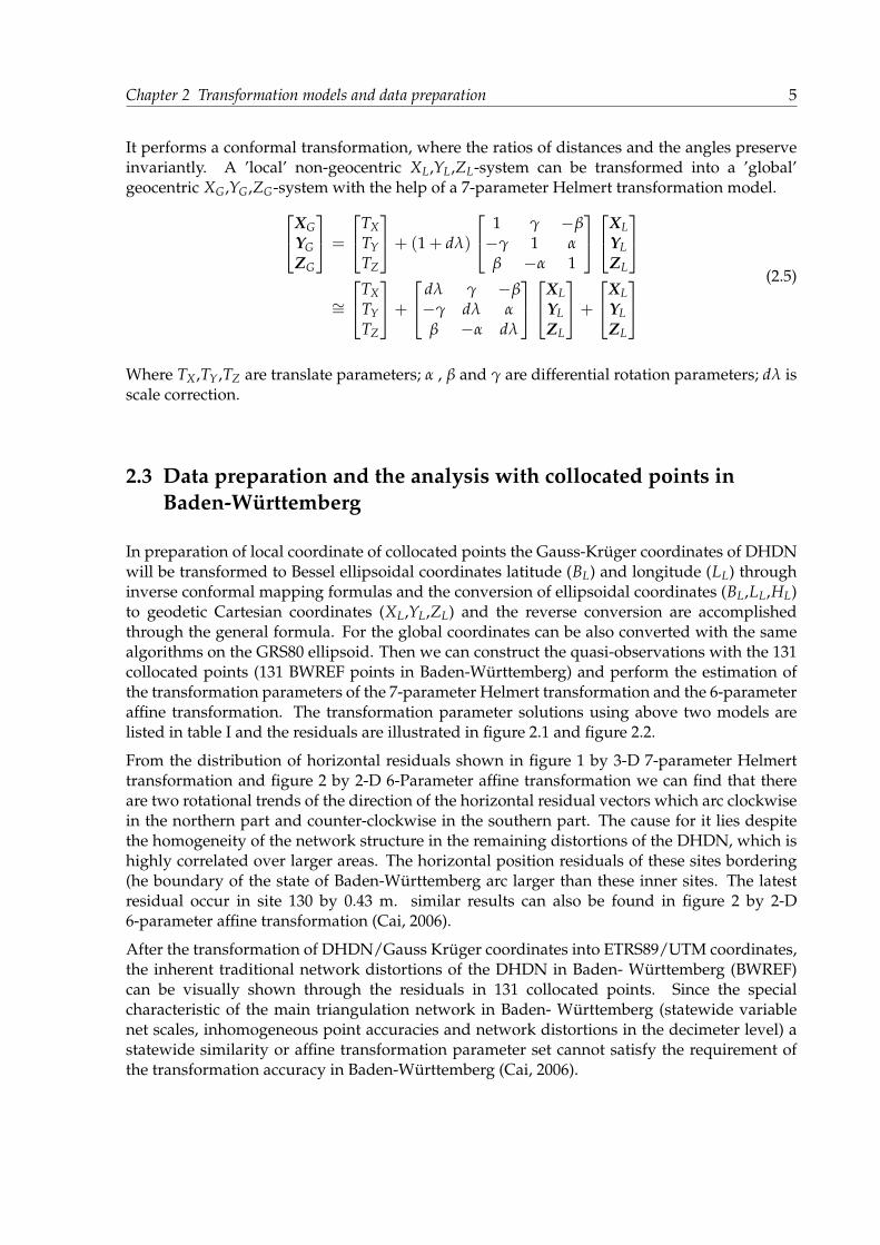
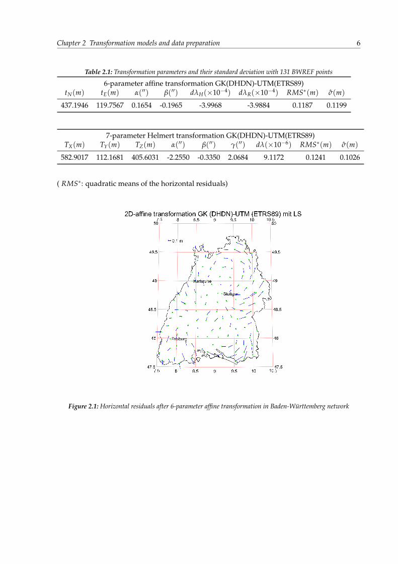
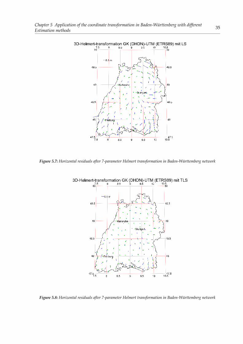
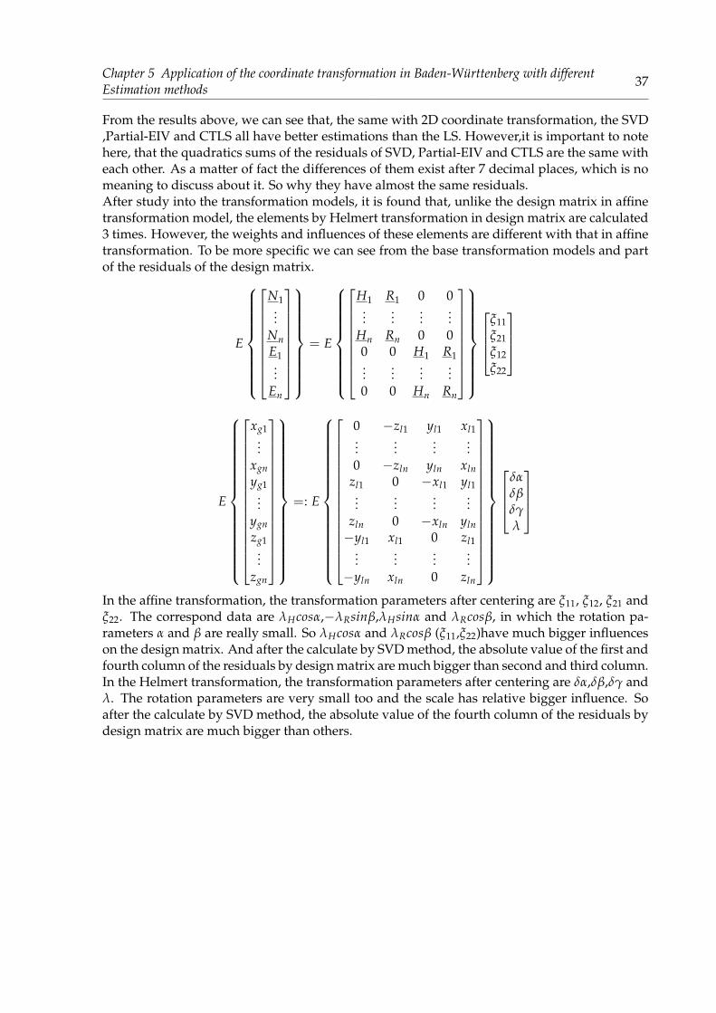
From the distribution of horizontal residuals shown in figure 1 by 3-D 7-parameter Helmerttransformation and figure 2 by 2-D 6-Parameter affine transformation we can find that thereare two rotational trends of the direction of the horizontal residual vectors which arc clockwisein the northern part and counter-clockwise in the southern part. The cause for it lies despitethe homogeneity of the network structure in the remaining distortions of the DHDN, which ishighly correlated over larger areas. The horizontal position residuals of these sites bordering(he boundary of the state of Baden-Württemberg arc larger than these inner sites. The latestresidual occur in site 130 by 0.43 m. similar results can also be found in figure 2 by 2-D6-parameter affine transformation (Cai, 2006).
After the transformation of DHDN/Gauss Krüger coordinates into ETRS89/UTM coordinates,the inherent traditional network distortions of the DHDN in Baden- Württemberg (BWREF)can be visually shown through the residuals in 131 collocated points. Since the specialcharacteristic of the main triangulation network in Baden- Württemberg (statewide variablenet scales, inhomogeneous point accuracies and network distortions in the decimeter level) astatewide similarity or affine transformation parameter set cannot satisfy the requirement ofthe transformation accuracy in Baden-Württemberg (Cai, 2006).
Chapter 2 Transformation models and data preparation 6
Table 2.1: Transformation parameters and their standard deviation with 131 BWREF points
6-parameter affine transformation GK(DHDN)-UTM(ETRS89)tN(m) tE(m) α(′′) β(′′) dλH(×10−4) dλR(×10−4) RMS∗(m) σ(m)
437.1946 119.7567 0.1654 -0.1965 -3.9968 -3.9884 0.1187 0.1199
7-parameter Helmert transformation GK(DHDN)-UTM(ETRS89)TX(m) TY(m) TZ(m) α(′′) β(′′) γ(′′) dλ(×10−6) RMS∗(m) σ(m)
582.9017 112.1681 405.6031 -2.2550 -0.3350 2.0684 9.1172 0.1241 0.1026
( RMS∗: quadratic means of the horizontal residuals)
Figure 2.1: Horizontal residuals after 6-parameter affine transformation in Baden-Württemberg network
Chapter 2 Transformation models and data preparation 7
Figure 2.2: Horizontal residuals after 7-parameter Helmert transformation in Baden-Württemberg network
8
Chapter 3
Total Least Squares
3.1 Introduction
The total least squares method is one of several linear parameter estimation techniques thathave been devised to compensate for data errors. The basic motivation for total least squares(TLS) is the following: Let a set of multidimensional data points (vectors) be given. How canone obtain a linear model that explains these data? The idea is to modify all data points insuch a way that some norm of the modification is minimized subject to the constraint that themodified vectors satisfy a linear relation. (Van Huffel, 1991)The origin of this basic idea can be traced back to the beginning of last century. It was redis-covered many times, often independently, mainly in the statistical and psychometric literature.However, it is only in the 1980s and 1990s that the technique also found wide use in scientificand engineering applications. One of the main reasons for its popularity is the availability ofefficient and numerical robust algorithms, in which the singular value decomposition plays aprominent role. Another reason is the fact the TLS is an application oriented procedure. It isideally suited for situations in which all data are corrupted by noise, which is almost alwaysthe case in engineering applications. In this sense, it is a powerful extension of the classicalleast squares method, which corresponds only to a partial modification of the data.The problem of linear parameter estimation arises in a broad class of scientific disciplines suchas signal processing, automatic control, system theory and in general engineering, statistics,physics, economics, biology, medicine, etc... It starts from a model described by a linearequation.
y = a1ξ1 + · · ·+ amξm (3.1)
Where a1, · · · , am and y denote the variables and ξ = [ξ1, · · · , ξm]T ∈ Rm plays role of a
parameter vector that characterizes the specific system. The basic problem is then to determinean estimate of the true but unknown parameters from certain measurements of the variables.This gives rise to an overdetermined set of m linear equations(m > n):
y = Aξ + ey (3.2)
Where the i − th row of the data matrix A ∈ Rm and the vector of observations y ∈ Rn
contain the measurements of the variables a1, · · · , am and y, respectively. In the classical leastsquares (LS) approach the measurements A of the variables ai (the right-hand side of (3.2)) areassumed to be free of error and hence, all errors are confined to the observation vector y (theleft-hand side of (3.2)). However, this assumption is frequently unrealistic: sampling errors,human errors, modelling errors and instrument errors may imply inaccuracies of the data
Chapter 3 Total Least Squares 9
matrix A as well. TLS is one method of fitting that is appropriate when there are errors in boththe observation vector y and the data matrix A. It amounts to fitting a ’best’ subspace to themeasurement data (AT
i , yi),i = 1, · · · , n, where ATi is the i− th row of A. To illustrate the effect
of TLS in comparison with LS, we consider here a simple example of parameter estimation,i.e., only one parameter (m = 1) is to be estimated. Hence, equation(3.1) reduces to
y = aξ (3.3)
An estimate for parameter ξ is to be found from n measurements of the variables a and y:
ai = a0i + ∆ai
yi = y0i + ∆yi i = 1, · · · , n
(3.4)
By solving the linear system (3.2) with A = [a1, · · · , an]T and b = [b1, · · · , bn]T. ∆ai and ∆yirepresent the random errors added to the true values a0
i and y0i of the variables a and y. If a
can be observed exactly, i.e., ∆ai = 0, errors only occur in the measurements of y contained inthe right-hand side vector y. Hence, the use of LS for solving (3.2) is appropriate. This methodperturbs the observation vector y by a minimum amount e so that (y− e) can be predicted byAξ. This is done by minimizing the sum of squared and differences
n
∑i=1
(yi − aiξ)2 (3.5)
The best estimate ξy of ξ follows then immediately:
ξy = (AT A)−1ATy =∑n
i=1 aiyi
∑ni=1 a2
i(3.6)
If y can be measured without error, i.e., ∆yi = 0, the use of LS is again appropriate. Indeed wecan rewrite as
yξ= a (3.7)
And confine all errors to the measurements of α contained in the right-hand side vector A ofthe corresponding set of equations A ≈ yξ−1. By minimizing the sum of squared differencesbetween the measured values ai and the predicted values yi/ξ, the best estimate ξA of ξ is givenby
ξy = (yTy)−1yT A =∑n
i=1 a2i
∑ni=1 aiyi
(3.8)
In many application, however, both variables are measured with errors, i.e., ∆ai 6= 0 and∆yi 6= 0. If the errors are independently and identically distributed with zero mean andcommon variance σ2
v , the best estimate ξ is obtained by minimizing the sum of squareddistances of the observed points from the fitted line, i.e.,
n
∑i=1
(yi − aiξ)2/(1 + ξ2) (3.9)
This is in fact the solution ξTLS we obtain by solving (3.2) with the TLS method for m = 1.
Chapter 3 Total Least Squares 10
3.2 Total Least Squares with singular value decomposition(SVD)
The singular value decomposition(SVD) is of great theoretical and practical importance forthe LS and TLS problems. Not only does it provide elegant geometrical and algebraic insightsinto many numerical linear algebra problems, but also at the same time, a numerically reliablealgorithm can be devised.
If C ∈ Rn×m then there exist orthonormal matrices U = [u1, · · · , un] ∈ Rn×m andV = [v1, · · · , vn] ∈ Rn×m such that (Van Huffel, 1991)
UTCV = ∑ = diag(σ1, · · · , σp), σ1 ≥ · · · ≥ σp ≥ 0 and p = min(n, m) (3.10)
The σi are are the singular values of C and they are collectively known as the singular valuespectrum. The vectors ui and vi are the i− th left singular vector and the i− th right singularvector, respectively. The triplet ui, sigmai, vi is called a singular triplet. It is easy to verify bycomparing columns in the equations CV = U ∑ and CTU = ∑T V that
Cvi = σiui and CTui = σivi i = 1, · · · , p (3.11)
The SVD reveals many interesting structures of a matrix. If the SVD of C is given by Theorem1, and we define r by
σ1 ≥ · · · ≥ σr ≥ σr+1 = · · · = σp = 0
the number of positive singular values, then
rank(C) = r,R(C) = R([u1, · · · , ur]),N(C) = R([vr+1, · · · , vm]),
Rr(C) = R(CT) = R([v1, · · · , vr]),
Nr(C) = N(CT) = R([ur+1, · · · , un]).
(3.12)
Moreover, if Ur = [u1, · · · , ur], ∑r = diag(σ1, · · · , σp) and Vr = [v1, · · · , vr], then we have theSVD expansion
C = Ur ∑r
V Tr =
r
∑i=1
σiuivTi (3.13)
Above equation, which is also called the dyadic decomposition, decomposes the matrix C ofrank r in a sum of r matrices of rank one. Also, the 2-norm an the Frobenius norm are neatlycharacterized in terms of the SVD:
‖C‖2F =
n
∑i=1
m
∑j=1
c2ij = σ2
1 + · · ·+ σ2p , p = min(n, m)
‖C‖2 = supy 6=0
‖Cy‖2‖y‖2
= σ1
Chapter 3 Total Least Squares 11
With Eckart-Young-Mirsky matrix approximation theorem, let the SVD of C ∈ Rn × m begiven by C = ∑r
i=1 σiuivTi with r = rank(C). If k < r and Ck = ∑k
i=1 σiuivTi , then
minrank(D)=k
‖C− D‖2 = ‖C− Ck‖2 = σk+1
minrank(D)=k
‖C− D‖F = ‖C− Ck‖F =
√√√√ p
∑i=k+1
σ2i , p = min(n, m)
(3.14)
Eckart and Young originally proved the theorem for the Frobenius norm in 1936. In 1960,Mirsky proved the theorem for the 2-norm. Therefore, Theorem 2 is called the Eckart-Young-Mirsky Theorem (Van Huffel, 1991).
On the basis of the above mathematical theorems, convert model Ax = b to[A b
] [ x−1
]= 0.
If it performs SVD on matrix[A b
], using the above theorem, following formulas can be
derived under the criteria∥∥[A; b
]−[A; b
]∥∥2 = min.
x = − 1vt+1,t+1
[v1,t+1 · · · vt+1,t+1]T
[∆A ∆b
]=[A b
]−[A b
]= σt+1ut+1vT
t+1
(3.15)
Where t is the number of parameters. Although this algorithm is based on established math-ematical theorems, it has a weakness. Golub and Van Loan presumed that A, b are stochasticelements and performed SVD directly on the matrix
[A b
]. However, some elements of A
may be non-stochastic, or some elements containing errors could appear more than once. Toperform the minimum norm constraint without this consideration is inappropriate and mayresult in large deviations.
3.3 Total Least Squares with the Euler-Lagrange approach
Another solution for TLS is the iterative method(Schaffrin, 2006). The most important featureof the iterative method is it’s straightforward algorithm. Schaffrin and Felus(2003) have intro-duced a multivariate version of Total Least Squares (TLS) adjustment in order to determine theoptimal parameters of an affine coordinate transformation empirically.
The following model, with full-rank matrix A, is assumed (Schaffrin, 2003):
(A− EA)ξ − (y− e) = 0E {[EA, e]} = 0C {[EA, e]} = 0
D {vec [EA, e]} = Σ0 ⊗ In
(3.16)

Chapter 3 Total Least Squares 12
Where e and EA denote a random error vector, resp. matrix. Σ0 = σ20 Im+1 is a (m+ 1)× (m+ 1)
matrix with an unknown variance component σ20 and given identity matrix Im+1. The symbol
⊗ denotes the ’Kronecker-Zehfuss product’ of matrices, defined by:
M ⊗ N :=[mij · N
]For M = mij and N arbitrary.
The ’vec’ operator stacks one column of a matrix under the other, moving from left to right. Incontrast to the Least-Squares(LS) method, this is based on the minimization of
eTe = (y− Aξ)T(y− Aξ) (3.17)
Under the condition EA = 0, the(equally weighted) TLS principle is based on minimizing theobjective function (Schaffrin, 2003):
eTe + (vecEA)T(vecEA) = min(ξ) (3.18)
When performing an adjustment, it is sometimes necessary to fix some parameters to spe-cific values. Here, a total least squares solution will be presented, along with an iterationscheme(Schaffrin, 2003).
In order to solve the TLS problem as presented in (3.18) and minimize the respective objectivefunction in view of the model (3.16), we define the Lagrange target function as follows where
eA : = vec(EA) ∼ (0, σ20 Im ⊗ In)
Φ(e, eA, λ, ξ) = eTe + eTAeA + 2λT [y− e− Aξ + EAξ]
(3.19)
Where λ denotes the n× 1 vector of Lagrange multipliers; note that
EAξ = (ξT ⊗ In)eA (3.20)
thus the Euler-Lagrange necessary conditions are (Schaffrin, 2003):
12
∂Φ
∂e= e− λ = 0
12
∂Φ
∂eA= eA − (ξ ⊗ In)λ = 0
12
∂Φ
∂λ= y− Aξ − e + EAξ = 0
12
∂Φ
∂ξ= −ATλ + ET
Aλ = 0
This system is simplified into:
(AT A)ξ = ATy + ξ(λTλ)(1 + ξT ξ)
λ = (e− EAξ)(1 + ξT ξ)−1 = (y− Aξ)(1 + ξT ξ)−1 (3.21)
Note that
v =(y− Aξ)T(y− Aξ)
(1 + ξT ξ)= (λTλ)(1 + ξT ξ) = eT e + ET
AEAξ = min(ξ) (3.22)
Chapter 3 Total Least Squares 13
is Rayleigh’s quotient for the matrix [AT A ATyyT A yTy
](3.23)
with[ξT,−1
]Tas the vector argument. Rayleigh’s quotient defines the minimum eigen-
value of the augmented matrix, based on the corresponding eigenvector(see, e.g.,G. Strang,1988)(Schaffrin, 2003).Using these equations the following algorithm had been developed by Schaffrin (2003) to solvethe TLS problem (Schaffrin, 2003):
1) Compute the LS solution:
ξ1 = (AT A)−1ATy ( f or v0 := 0)
2) Insert the solution of step 1) as the innitial value for the following iterative process:
ξi+1 = (AT A)−1[ATy +(y− Aξi)T(y− Aξi)
(1 + (ξi)T ξi)]
3) End when∥∥∥ξi+1 − ξi
∥∥∥ < ε. Then
σ20 =
v(n−m)
The algorithm seems to converge to the TLS solution in most cases although it’s efficiency(convergence rate, convergence radius, etc.) still needs to be further investigated. However,since the iterative method is the gradual approximation of the true value of parameter, iterativesolutions can be a problem if there is a high degree of nonlinearity.
3.4 Total Least Squares based on Partial-EIV model
Total Least Squares has attracted a widely spread attention since Golub and van Loan (1980)coined the terminology of Total Least Squares and demonstrated that the TLS solution can bereadily obtained algorithmically by singular value decomposition about 30 years ago. TheTotal Least squares method has been developed to deal with observation equations, whichare functions of both unknown parameters of interest and other measured data contaminatedwith random errors. Such an observation model is well known as an errors-in-variables (EIV)model and almost always solved as a nonlinear equality-constrained adjustment problem. Xu,Liu and Shi (2012) reformulate it as a nonlinear adjustment model without constraints andfurther extend it to a Partial-EIV model, in which not all the elements of the design matrixare random. As a result, the total number of unknowns in the normal equations has beensignificantly reduced.
The EIV observation model is defined as:
y− ey = (A− EA)ξ (3.24)
Chapter 3 Total Least Squares 14
Where y denotes the m × 1 observation vector, A represents the the m × n coefficient matrixwith rank(A) = n < m. ξ represents the n × 1 unknown parameter vector. Moreover, eydenotes the random error vector of y, and EA denotes the random error matrix of A. ey is oftensupposed to be of zero mean and a variance-covariance matrix σ2
0 Qy , with Qy being a givenpositive definite cofactor matrix and σ2
0 an variance of unit weight. eA = vecEA, in which ’vec’denotes the operator which stacks one column of the matrix underneath the previous one, eAis also assumed to be zero mean and the variance-covariance matrix is defined as σ2
0 Qy , withQA being the cofactor matrix of eA, QA is singular when the matrix A contains non-randomelements. ey and eA is uncorrelated.
Xu etal.(2012) transformed the EIV model into a partial-EIV model by extracting functionallyindependent random variables within the coefficient matrix:
y− ey = (ξT ⊗ Im) [h + B(a− ea)] (3.25)
where Im is the m − th order identity matrix, a is a t × 1 vector of functionally independentvariables within A, ea denotes the random error vector of a, h is a deterministic constantvector whose elements correspond to the non-random elements of A, B is a given deterministicmatrix with a dimension of mn× t. Obviously, A can be expressed as:
A = ivec(h + Ba) (3.26)
where ’ivec’ represents the inverse operator of ’vec’ , which recovers the mn× 1 vector to theoriginal matrix with a dimension of m× n.The corresponding stochastic model of the partial EIV model is:[
eyea
]∼([
00
]σ2
0
[Qy 00 Qa
])(3.27)
where Qa denotes a given positive definite cofactor matrix of ea.We assume that the obtained parameter estimator vector after i − th iteration is ξ(i), and thepredictive residual vector of a is ea(i). The right-hand member of (3.25) is expressed through
Taylor series expansion at(
X(i), ea(i)
):
y− ey =(
XT(i) ⊗ Im
)(h + Ba)−
(XT(i) ⊗ Im
)Bea + ivec(h + B(a− ea(i)))δξ
= Aξ(i) + A(i)δξ − (ξT(i) ⊗ Im)Bea
(3.28)
whereA(i) = ivec(h + B(a− ea(i))) = A− ivec(Bea(i)) (3.29)
In (3.28), the terms of the second and higher orders are omitted, whereas only the first orderterms are maintained. δξ denotes the small corrected values of ξ.The Lagrange objective function of TLS is constructed as:
Φ(ey, ea, ξ, λ) =
eTy Q−1
L ey + eTa Q−1
a ea + 2λT(y− ey − Aξ(i) − A(i)δξ + (ξT(i) ⊗ Im)Bea)
(3.30)
Chapter 3 Total Least Squares 15
where λ is the m× 1 vector of ’Lagrange multipliers’, the solution of this target function can bederived via the Euler-Lagrange necessary conditions:
12
∂Φ
∂ey= Q−1
L e− λ = 0
12
∂Φ
∂ea= Q−1
a ea + BT(ξ(i) ⊗ Im)λ = 0
12
∂Φ
∂ξ= −AT
(i)λ = 0
12
∂Φ
∂λ= y− Aξ(i) − ey + (ξT
(i) ⊗ Im)Bea = 0
(3.31)
The following equations are derived though solving (3.31):
δξ(i+1) = (AT(i)Q
−1c(i)A(i))
−1AT(i)Q
−1c(i)(y− Aξ(i)) (3.32)
withξ(i+1) = δξ(i+1) + ξ(i)
then we get the new ξ(i+1)
δξ(i+1) = (AT(i)Q
−1c(i)A(i))
−1AT(i)Q
−1c(i)(y− (ξT
(i) ⊗ Im)Bea(i)) (3.33)
ey(i+1) = QyQ−1c(i)(y− Aξ(i) − A(i)δξ(i+1)) (3.34)
ea(i+1) = QaBT(ξ(i) ⊗ Im)Q−1c(i)(y− Aξ(i) − A(i)δξ(i+1)) (3.35)
In equations (3.35-3.38),
Qc(i) = Qy + (ξT(i) ⊗ Im)BQaBT(ξ(i) ⊗ Im) (3.36)
The iterative process described in equations (3.32-3.35) can be implemented from LS solution.A small positive number threshold ε should be primarily presented to terminate iteration until∥∥∥δ ˆξ(i+1)
∥∥∥ < ε , where ‖·‖ represents l2-norm of a vector. This algorithm reduced the number ofunknowns and directly deal with the positive cofactor matrix Qa instead of QA. However, wecan see from the equations above that, the mathematical algorithm is very complicate. Whichmakes it quite difficult to grasp.
16
Chapter 4
Converted Total Leat Squares
4.1 Introduction and mathematical foundation
The Converted Total Least Squares (CTLS) is proposed for dealing with the errors-in-variables(EIV) model. Firstly take classic Gauss-Markov model of LS as basis equation.
y = Aξ + ey (4.1)
Taking into account the design matrix’s errors in model (4.1) will lead to difficulties forparameter estimation and accuracy assessment. Particularly, one cannot apply the traditionalerror propagation law directly, since die law is established on the basis of linear relations.The basic idea of CTLS is to take the stochastic design matrix elements as virtual observation.On the basis of the original error equation, the number of observation equation is increased bytaking the design matrix elements as the observation vector, and some of the design matrixelements are estimated as parameters in the new algorithm. The advantage of such strategyis the ability to obtain the adjusted value of required parameters, the design matrix is formedby the initial value of design matrix parameters, which no longer has random properties. Theparameters obtained are the linear functions of the observation vector. After this treatment,(4.1) is combined with the classical LS adjustment theory.Augmenting the observation equations that take design matrix elements as virtual observationon the basis of the original error equation.
ya = ξa + ea (4.2)

Chapter 4 Converted Total Leat Squares 17
Figure 4.1: Illustrate the basic idea of the algorithm
Where ya is comprised of the design matrix elements that contain errors, and ξa is comprisedof the new parameters. If (4.1)is combine with (4.2), a mathematical model under the newalgorithm can be obtained.
y = Aξ + ey
ya = ξa + ea(4.3)
It should be clear that ya contains only the observations of design matrix. To distinguish thedesign matrix in the original model, the symbol Aξ is used to denote the design matrix in (4.1),which is formed by the initial value of parameters ξa and some elements without errors.
Chapter 4 Converted Total Leat Squares 18
Based on the above model, we can get the following error equations
ey = (A0ξ + EA)(ξ0 + ∆ξ)− y
= A0ξ∆ξ + EAξ0 + A0
ξξ0− y + ∆A∆ξ → EA∆ξ ≈ 0
= A0ξ∆ξ + B∆a + A0
ξξ0− y
ea = a− ya
(4.4)
Where EA is composed of ∆a, the corrections to the new parameters, and B∆a is the rewrittenform of EAξ0. In converting EAξ0 to B∆a , which is the key step for the approach. A0
ξ iscomposed of non-stochastic elements in the design matrix and the initial value a.
Define η =
[y− A0
ξξ0
a− ya
], Aη =
[A0
ξ B0 E
], ∆η =
[∆ξ∆a
], eη =
[eyea
], (4.5) can be reduced to:
η = Aη∆η+ eη (4.5)
Where eη is the residual vector of all observations, Aη is formed by the initial values of theparameters, and ∆η is comprised of the corrections to all parameters. The estimation criterionis still eT
η eη → min, which is the same as eTy ey + eT
η eη → min. Since the TLS problem istransformed into the classical LS problem, the adjustment can be completed by following the
classical LS principle. The new weight matrix is Pη =
[Py 00 Pa
]. And the TLS problem can be
solved considering the weight of observations and stochastic design matrix by:
∆η = (ATη PηAη)
−1ATη Pηη (4.6)
4.2 Estimation formula of unit weight variance
The estimation formula of unit weight variance of the TLS is difficult to determine. Inconsidering the design matrix errors, the question of whether or not the degree of freedom foradjustment model changes arises. The TLS problem is converted into a classical LS problemusing the new algorithm. With model (4.6), after adjustment by the LS principle, and V asthe correct ion of observations, accuracy assessment is straightforward from the adjustmenttheory. (4.8) is the resulting formula of unit weight variance for TLS.
σ20 =
ATη PηAη
tr(PηQVV)=
ATη PηAη
(n + u)− (t + u)=
ATη PηAη
n− t(4.7)
where n is the number of observations that the observation vector y contains, u is the numberof stochastic elements in the design matrix A. t is the number of parameters, here only thenumber of original parameters in model (4.1). u ≤ n× t and tr(PηQVV) = (n + u)− (t + u) isthe conclusion of the Gauss-Markov theorem.Compared with LS, the degree of freedom for TLS does not change, that is, TLS and LS havethe same degrees of freedom.

Chapter 4 Converted Total Leat Squares 19
4.3 Co-factor matrix of parameters
Giving the error description of parameters is a basic object of adjustment. The TLS accuracyassessment problem is difficult to resolve in TLS adjustment theory. For decades, manyscholars have proposed different methods to do so. However, these methods vary in termsof degrees of approximation, such that real statistical information of parameters cannot beobtained. CTLS allows TLS accuracy assessment through the theory of classical LS accuracyassessment.After the adjustment based on model (4.6), the design matrix is formed by the initial value ofdesign matrix parameters since it no longer has random properties, and accuracy assessmentcan continue based on the principle of error propagation The co-factor of parameters may betaken as an example below:
Q∆η′∆η′ = (ATη PηAη)
−1ATη PηQηPηB(BT PηB)−1 = (AT
η PηAη)−1 (4.8)
Solving TLS problems by CTLS does not only solve the TLS accuracy assessment problem,which limit the expanded use of TLS, but also achieves integration of the TLS theory with theclassical LS approach.
Appendix Vectorization of the matrix product equation
Vec(ABC) = (CT ⊗ A)Vec(B)
ABX = Vec(ABX) = Vec(XT BT AT)
ABX = (XT ⊗ A)Vec(B)
If An·n
= I, Bn·t
, then
In·n
Bn·t
X = (XT ⊗ I)t·1
Vec(B)
And
Bn·t
Xt·1
= (XT ⊗ I)n⊗np
Vec(B)np·1
20
Chapter 5
Application of the coordinate transformation inBaden-Württenberg with different Estimationmethods
5.1 Transformation in two-dimensional(2D)
Before we transform the coordinate, we need to centralize the 6-parameter affine transforma-tion model in order to vanish the translation parameters.[
NE
]=
[λHcosα −λRsinβλHsinα λRcosβ
] [HR
]+
[tNtE
]
=:[
ξ11 ξ21ξ12 ξ22
] [HR
]+
[ξ31ξ32
]=
[H R 0 0 1 00 0 H R 0 1
]
ξ11ξ21ξ12ξ22ξ31ξ32
(5.1)
Because the element ’1’ and ’0’ have no error, the translation parameters shall disappearby centering this equation. Thus, after the centering the coordinates in the mid point, thetranslation parameters tN and tE will be automatically vanished. Then the observation and oldcoordinates are centered on their average values in the form:[
NE
]=:[
ξ11 ξ21ξ12 ξ22
] [HR
](5.2)
with
N = N −mean(N), E = E−mean(E)H = H −mean(H), R = R−mean(R)

Chapter 5 Application of the coordinate transformation in Baden-Württenberg with differentEstimation methods 21
Figure 5.1: Illustrate the process for 6p-affine transformation
5.1.1 Transformation with Total Least Squares(SVD)
For the n couple of coordinates we have the transformation model, which is suited for theapplication of TLS solution.
E
N1...
NnE1...
En
= E
H1 R1 0 0...
......
...Hn Rn 0 00 0 H1 R1...
......
...0 0 Hn Rn
ξ11ξ21ξ12ξ22
y− e = (A− EA)ξ (5.3)
eT e + ETAEA = min(e, EA, ξ) (5.4)
Solution of the TLS problem by using the singular value decomposition(SVD).
ξTLS = (AT A− σ2m+1I)−1AT y (5.5)
with σm+1 the smallest singular value of the augmented design matrix [A; y]:
[A; y] = UΣV T =m+1
∑∑∑i=0
σiuivTi , σ1 ≥ · · · ≥ σm+1 ≥ 0
The best TLS approximation [A; y] of [A; y] is give by
[A; y] = UΣV T , with Σ = diag(σ1, · · ·, σm, 0)
and with corresponding TLS correction matrix
[EA; e] = [A; y]− [A; y] = σm+1um+1vTm+1
With MATLAB function [U,S,V]=svd(X) these procedures can be implemented easily.We can see from the design matrix A that, the elements H i and Ri appeared twice, which means
Chapter 5 Application of the coordinate transformation in Baden-Württenberg with differentEstimation methods 22
their corrections have been calculated twice. Additionally, the element 0 also have correctionwhen we perform SVD method. 0 is a non-stochastic element and theoretically has no correc-tion. This means that SVD has a theoretical weakness in that it can not be applied directly whenonly part of the design matrix contains errors.
5.1.2 Transformation with Total Least Squares based on Partial-EIV model
For the n couple of coordinates we have the same transformation model, which is suited forthe application of TLS solution.
E
N1...
NnE1...
En
= E
H1 R1 0 0...
......
...Hn Rn 0 00 0 H1 R1...
......
...0 0 Hn Rn
ξ11ξ21ξ12ξ22
Reform the EIV observation model from
y− ey = (A− EA)ξ
to
y− ey = (ξT ⊗ Im) [h + B(a− ea)] (5.6)
Create the vector a, h and the deterministic matrix B
a(2n×1)
=
H1...
HnR1...
Rn
h = 0
B(8n×2n)
=
In 00 00 In0 00 0In 00 00 In
with In =
1 0 0
0. . . 0
0 0 1
= n, 0 =
0 0 0
0. . . 0
0 0 0
= n
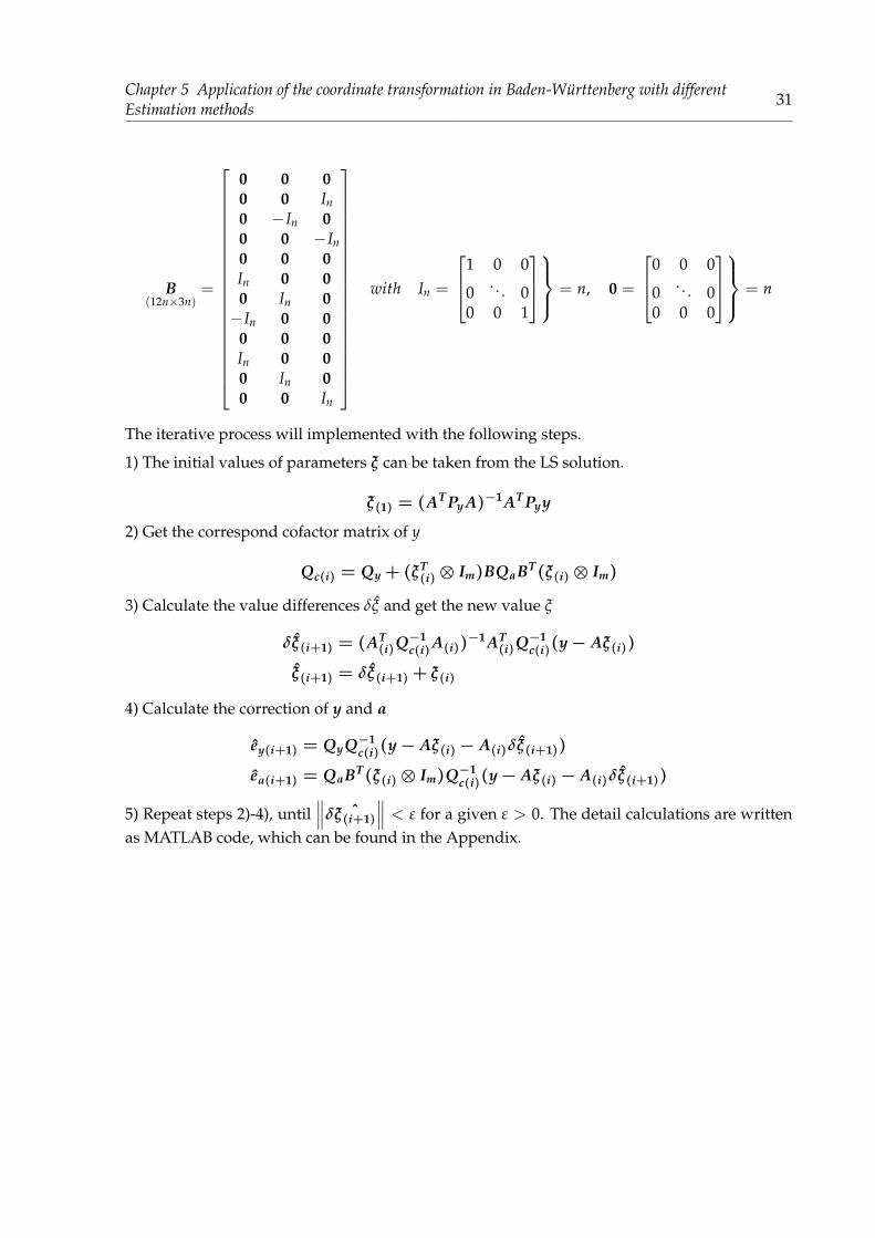
The iterative process will implemented with the following steps.
1) The initial values of parameters ξ can be taken from the LS solution.
ξ(1) = (AT Py A)−1AT Pyy
Chapter 5 Application of the coordinate transformation in Baden-Württenberg with differentEstimation methods 23
2) Get the correspond cofactor matrix of y
Qc(i) = Qy + (ξT(i)⊗ Im)BQaBT(ξ(i)⊗ Im)
3) Calculate the value differences δξ and get the new value ξ
δξ(i+1) = (AT(i)Q−1
c(i)A(i))−1AT
(i)Q−1c(i)(y− Aξ(i))
ξ(i+1) = δξ(i+1) + ξ(i)
4) Calculate the correction of y and a
ey(i+1) = QyQ−1c(i)(y− Aξ(i)− A(i)δξ(i+1))
ea(i+1) = QaBT(ξ(i)⊗ Im)Q−1c(i)(y− Aξ(i)− A(i)δξ(i+1))
5) Repeat steps 2)-4), until∥∥∥δ ˆξ(i+1)
∥∥∥ < ε for a given ε > 0. The detail calculations are writtenas MATLAB code, which can be found in the Appendix.
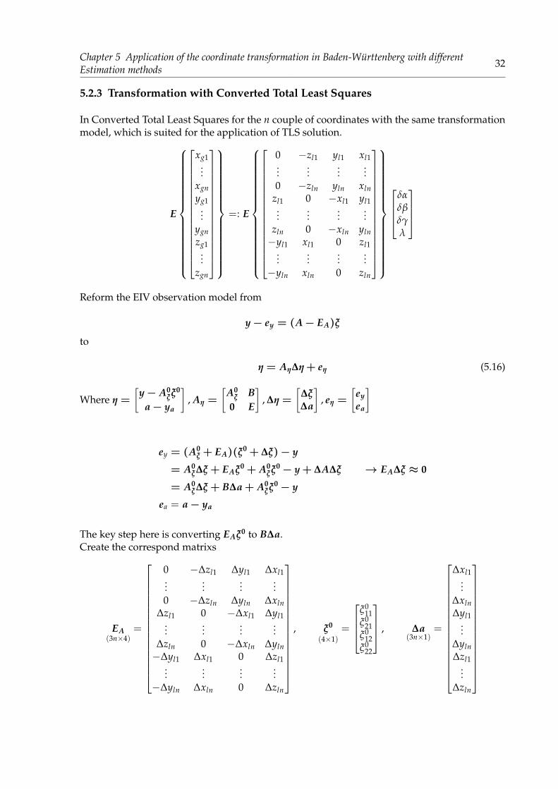
5.1.3 Transformation with Converted Total Least Squares
In Converted Total Least Squares for the n couple of coordinates with the same transformationmodel, which is suited for the application of TLS solution.
E
N1...
NnE1...
En
= E
H1 R1 0 0...
......
...Hn Rn 0 00 0 H1 R1...
......
...0 0 Hn Rn
ξ11ξ21ξ12ξ22
Reform the EIV observation model from
y− ey = (A− EA)ξ
to
η = Aη∆η+ eη (5.7)
Where η =
[y− A0
ξξ0
a− ya
], Aη =
[A0
ξ B0 E
], ∆η =
[∆ξ∆a
], eη =
[eyea
]
ey = (A0ξ + EA)(ξ0 + ∆ξ)− y
= A0ξ∆ξ + EAξ0 + A0
ξξ0− y + ∆A∆ξ → EA∆ξ ≈ 0
= A0ξ∆ξ + B∆a + A0
ξξ0− y
ea = a− ya
Chapter 5 Application of the coordinate transformation in Baden-Württenberg with differentEstimation methods 24
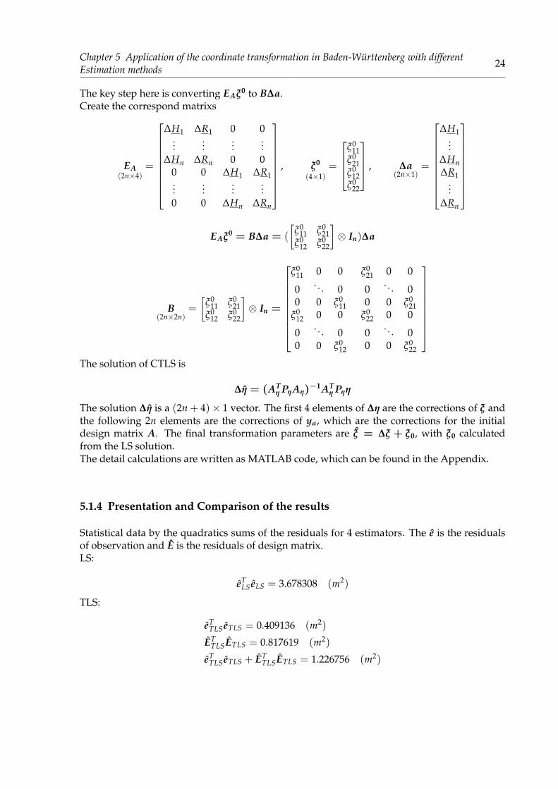
The key step here is converting EAξ0 to B∆a.Create the correspond matrixs
EA(2n×4)
=
∆H1 ∆R1 0 0...
......
...∆Hn ∆Rn 0 0
0 0 ∆H1 ∆R1...
......
...0 0 ∆Hn ∆Rn
, ξ0
(4×1)=
ξ0
11ξ0
21ξ0
12ξ0
22
, ∆a(2n×1)
=
∆H1...
∆Hn∆R1
...∆Rn
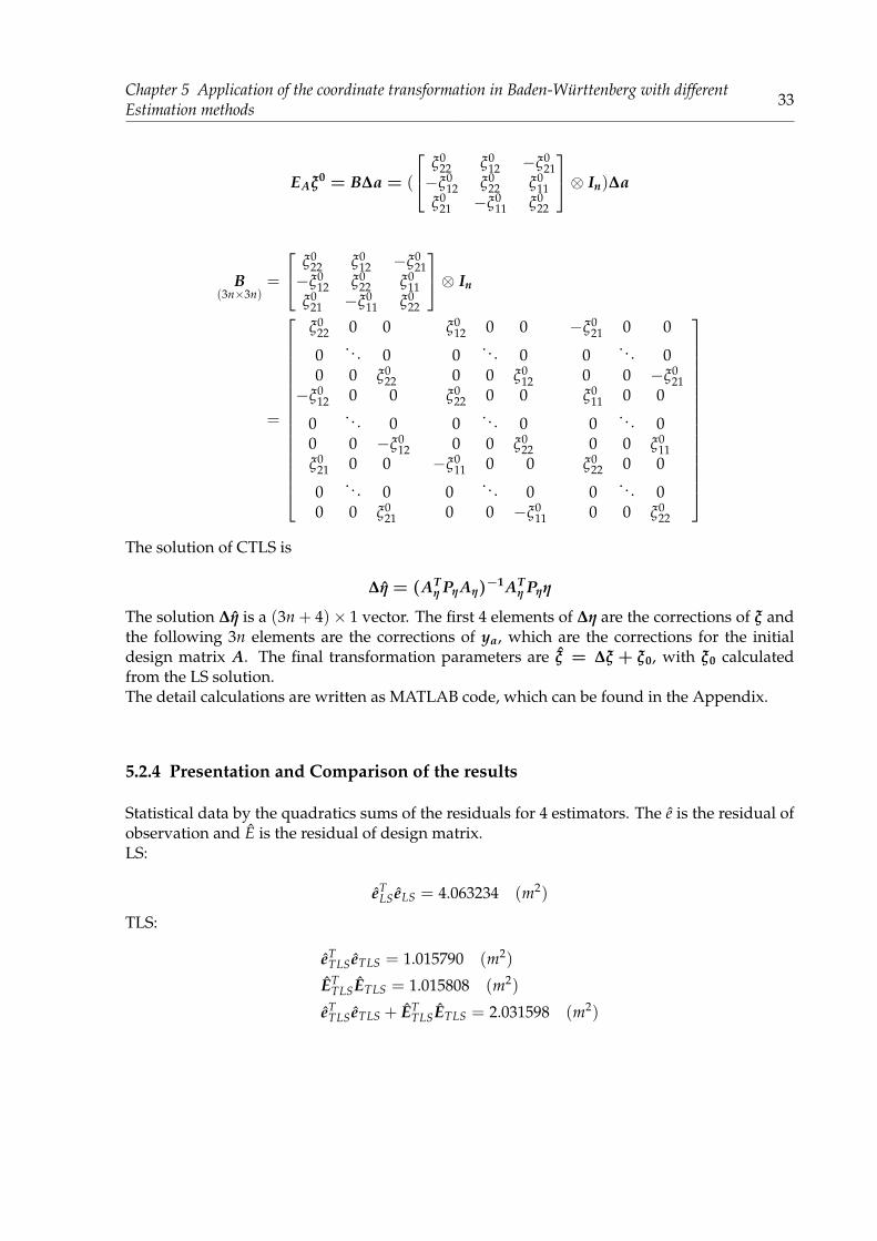
EAξ0 = B∆a = (
[ξ0
11 ξ021
ξ012 ξ0
22
]⊗ In)∆a
B(2n×2n)
=
[ξ0
11 ξ021
ξ012 ξ0
22
]⊗ In =
ξ011 0 0
0. . . 0
0 0 ξ011
ξ021 0 0
0. . . 0
0 0 ξ021
ξ012 0 0
0. . . 0
0 0 ξ012
ξ022 0 0
0. . . 0
0 0 ξ022
The solution of CTLS is
∆η = (ATη PηAη)
−1ATη Pηη
The solution ∆η is a (2n + 4)× 1 vector. The first 4 elements of ∆η are the corrections of ξ andthe following 2n elements are the corrections of ya, which are the corrections for the initialdesign matrix A. The final transformation parameters are ξ = ∆ξ + ξ0, with ξ0 calculatedfrom the LS solution.The detail calculations are written as MATLAB code, which can be found in the Appendix.
5.1.4 Presentation and Comparison of the results
Statistical data by the quadratics sums of the residuals for 4 estimators. The e is the residualsof observation and E is the residuals of design matrix.LS:
eTLS eLS = 3.678308 (m2)
TLS:
eTTLS eTLS = 0.409136 (m2)
ETTLSETLS = 0.817619 (m2)
eTTLS eTLS + ET
TLSETLS = 1.226756 (m2)

Chapter 5 Application of the coordinate transformation in Baden-Württenberg with differentEstimation methods 25
TLSP:
eTTLSP eTLSP = 0.920311 (m2)
ETTLSPETLSP = 0.919577 (m2)
eTTLSP eTLSP + ET
TLSPETLSP = 1.839889 (m2)
CTLS:
eTCTLS eCTLS = 0.920311 (m2)
ETCTLSECTLS = 0.919577 (m2)
eTCTLS eCTLS + ET
CTLSECTLS = 1.839889 (m2)
Table 5.1: Comparison of 6-parameter affine transformation parameters with 4 estimators
Transformation 6-parameter affine transformation GK(DHDN)-UTM(ETRS89)models tN(m) tE(m) α(′′) β(′′) dλH(×10−4) dλR(×10−4)
LS 437.194567 119.756709 0.165368 -0.196455 -3.996797 -3.988430TLS 437.194554 119.756712 0.165368 -0.196455 -3.996797 -3.988430
Partial-EIV 437.194556 119.756709 0.165375 -0.196445 -3.996797 -3.988430CTLS 437.194556 119.756709 0.165375 -0.196445 -3.996797 -3.988430
Table 5.2: Numerical deviation of 6-parameter affine transformation with 4 estimators
Transformationmodel
Collocatedsites
Absolute mean ofResiduals (m)
Max.absolute meanof Residuals(m)
RMS(m)
Standard deviationof unit weight (m)
[VN ] [VE] [VN ] [VE]
LS B-W 131 0.1049 0.0804 0.3288 0.3226 0.1187 0.1199TLS B-W 131 0.0350 0.0268 0.1097 0.1076 0.0396 0.0400
Partial-EIV B-W 131 0.0525 0.0402 0.1645 0.1614 0.0594 0.0848CTLS B-W 131 0.0525 0.0402 0.1645 0.1614 0.0594 0.0848
Chapter 5 Application of the coordinate transformation in Baden-Württenberg with differentEstimation methods 26
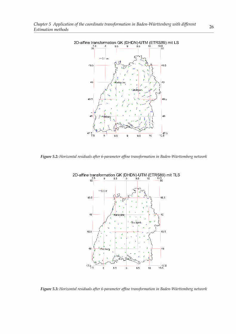
Figure 5.2: Horizontal residuals after 6-parameter affine transformation in Baden-Württemberg network
Figure 5.3: Horizontal residuals after 6-parameter affine transformation in Baden-Württemberg network

Chapter 5 Application of the coordinate transformation in Baden-Württenberg with differentEstimation methods 27
Figure 5.4: Horizontal residuals after 6-parameter affine transformation in Baden-Württemberg network
Figure 5.5: Horizontal residuals after 6-parameter affine transformation in Baden-Württemberg network
Chapter 5 Application of the coordinate transformation in Baden-Württenberg with differentEstimation methods 28
From the results above, we can see that the SVD, Partial-EIV and CTLS all have better estima-tions than the LS, which is obvious and reasonable. It should be pointed out that, it seems thatSVD has a better results than Partial-EIV and CTLS. Which is not correct, because the SVD is amethod taking the whole elements in design matrix into consideration. Under the same weightconditions, the deviation is systematically distributed to every element in the design matrix,even those non-stochastic elements included. As a consequence, the residuals calculated withSVD are not that dispersion. For the Partial-EIV and CTLS, they have almost the same results inevery part of estimation data. That means CTLS can calculate the 2 dimensional transformationparameters without iteration and has the same level of accuracy with Partial-EIV.
5.2 Transformation in three-dimensional(3D)
The following formula has been used for the estimation of the parameters in seven-parameterHelmert transformation.XG
YGZG
= (1 + dλ)
1 γ −β−γ 1 αβ −α 1
XLYLZL
+
TXTYTZ
XG = λ
1 γ −β−γ 1 αβ −α 1
XL + TL
(5.8)
Where λ is scale factor, α, β, γ are rotation angles. The translation terms TX, TY, TZ are thecoordinates of the origin of the 3-D network.After the linearization, the formula is rewritten:
XGYGZG
=
1 0 0 0 −ZL YL XL0 1 0 ZL 0 −XL YL0 0 1 −YL XL 0 ZL
TXTYTZδαδβδγλ
(5.9)
After centering the coordinates in the midpoints, the translation parameter TX, TY, TZ willdisappear, and then the observations and old coordinates are centered on their average values.This will be assumed in the following:
xgygzg
=
0 −zl yl xlzl 0 −xl yl−yl xl 0 zl
δαδβδγλ
(5.10)
with xgygzg
=
XGYGZG
−mean
XGYGZG
,
xlylzl
=
XLYLZL
−mean
XLYLZL
(5.11)
Chapter 5 Application of the coordinate transformation in Baden-Württenberg with differentEstimation methods 29
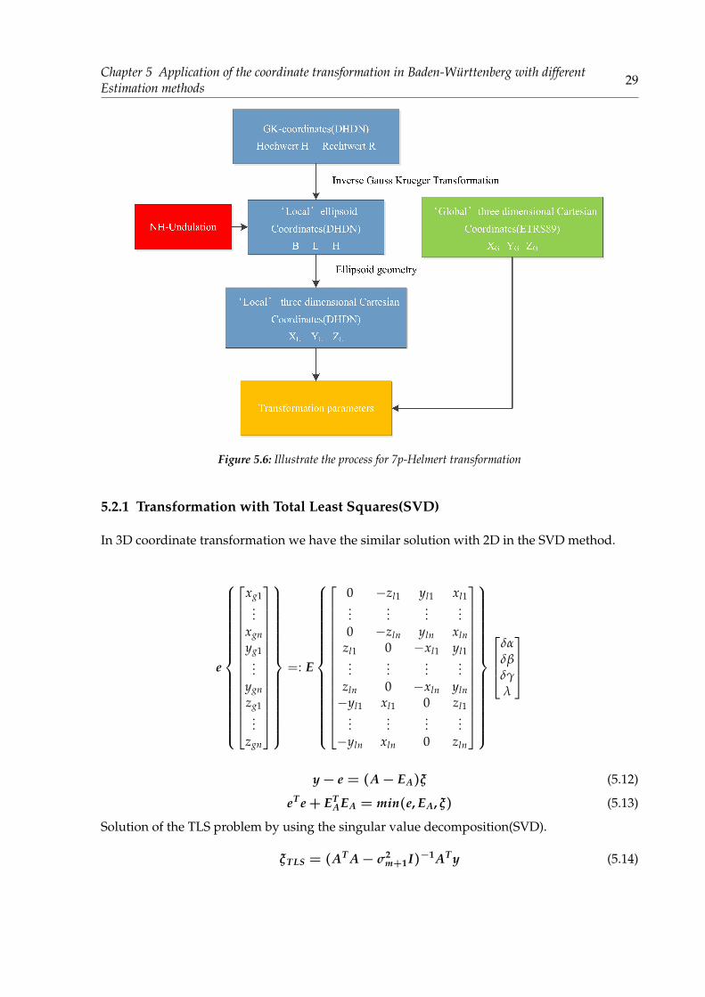
Figure 5.6: Illustrate the process for 7p-Helmert transformation
5.2.1 Transformation with Total Least Squares(SVD)
In 3D coordinate transformation we have the similar solution with 2D in the SVD method.
e
xg1...
xgnyg1
...ygnzg1
...zgn
=: E
0 −zl1 yl1 xl1...
......
...0 −zln yln xln
zl1 0 −xl1 yl1...
......
...zln 0 −xln yln−yl1 xl1 0 zl1
......
......
−yln xln 0 zln
δαδβδγλ
y− e = (A− EA)ξ (5.12)
eT e + ETAEA = min(e, EA, ξ) (5.13)
Solution of the TLS problem by using the singular value decomposition(SVD).
ξTLS = (AT A− σ2m+1I)−1AT y (5.14)

Chapter 5 Application of the coordinate transformation in Baden-Württenberg with differentEstimation methods 30
with σm+1 the smallest singular value of the augmented design matrix [A; y]:
[A; y] = UΣV T =m+1
∑∑∑i=0
σiuivTi , σ1 ≥ · · · ≥ σm+1 ≥ 0
The best TLS approximation [A; y] of [A; y] is give by
[A; y = UΣV T , with Σ = diag(σ1, · · ·, σm, 0)
and with corresponding TLS correction matrix
[EA; e] = [A; y]− [A; y] = σm+1um+1vTm+1
5.2.2 Transformation with Total Least Squares based on Partial-EIV model
For the n couple of coordinates we have the transformation model, which is suited for theapplication of TLS solution.
E
xg1...
xgnyg1
...ygnzg1
...zgn
=: E
0 −zl1 yl1 xl1...
......
...0 −zln yln xln
zl1 0 −xl1 yl1...
......
...zln 0 −xln yln−yl1 xl1 0 zl1
......
......
−yln xln 0 zln
δαδβδγλ
Reform the EIV observation model from
y− ey = (A− EA)ξ
to
y− ey = (ξT ⊗ Im) [h + B(a− ea)] (5.15)
Create the vector a, h and the deterministic matrix B
a(3n×1)
=
xl1...
xlnyl1...
ylnzl1...
zln
h = 0
Chapter 5 Application of the coordinate transformation in Baden-Württenberg with differentEstimation methods 31
B(12n×3n)
=
0 0 00 0 In0 −In 00 0 −In0 0 0In 0 00 In 0−In 0 0
0 0 0In 0 00 In 00 0 In
with In =
1 0 0
0. . . 0
0 0 1
= n, 0 =
0 0 0
0. . . 0
0 0 0
= n
The iterative process will implemented with the following steps.
1) The initial values of parameters ξ can be taken from the LS solution.
ξ(1) = (AT Py A)−1AT Pyy
2) Get the correspond cofactor matrix of y
Qc(i) = Qy + (ξT(i)⊗ Im)BQaBT(ξ(i)⊗ Im)
3) Calculate the value differences δξ and get the new value ξ
δξ(i+1) = (AT(i)Q−1
c(i)A(i))−1AT
(i)Q−1c(i)(y− Aξ(i))
ξ(i+1) = δξ(i+1) + ξ(i)
4) Calculate the correction of y and a
ey(i+1) = QyQ−1c(i)(y− Aξ(i)− A(i)δξ(i+1))
ea(i+1) = QaBT(ξ(i)⊗ Im)Q−1c(i)(y− Aξ(i)− A(i)δξ(i+1))
5) Repeat steps 2)-4), until∥∥∥δ ˆξ(i+1)
∥∥∥ < ε for a given ε > 0. The detail calculations are writtenas MATLAB code, which can be found in the Appendix.
Chapter 5 Application of the coordinate transformation in Baden-Württenberg with differentEstimation methods 32
5.2.3 Transformation with Converted Total Least Squares
In Converted Total Least Squares for the n couple of coordinates with the same transformationmodel, which is suited for the application of TLS solution.
E
xg1...
xgnyg1
...ygnzg1
...zgn
=: E
0 −zl1 yl1 xl1...
......
...0 −zln yln xln
zl1 0 −xl1 yl1...
......
...zln 0 −xln yln−yl1 xl1 0 zl1
......
......
−yln xln 0 zln
δαδβδγλ
Reform the EIV observation model from
y− ey = (A− EA)ξ
to
η = Aη∆η+ eη (5.16)
Where η =
[y− A0
ξξ0
a− ya
], Aη =
[A0
ξ B0 E
], ∆η =
[∆ξ∆a
], eη =
[eyea
]
ey = (A0ξ + EA)(ξ0 + ∆ξ)− y
= A0ξ∆ξ + EAξ0 + A0
ξξ0− y + ∆A∆ξ → EA∆ξ ≈ 0
= A0ξ∆ξ + B∆a + A0
ξξ0− y
ea = a− ya
The key step here is converting EAξ0 to B∆a.Create the correspond matrixs
EA(3n×4)
=
0 −∆zl1 ∆yl1 ∆xl1...
......
...0 −∆zln ∆yln ∆xln
∆zl1 0 −∆xl1 ∆yl1...
......
...∆zln 0 −∆xln ∆yln−∆yl1 ∆xl1 0 ∆zl1
......
......
−∆yln ∆xln 0 ∆zln
, ξ0
(4×1)=
ξ0
11ξ0
21ξ0
12ξ0
22
, ∆a(3n×1)
=
∆xl1...
∆xln∆yl1
...∆yln∆zl1
...∆zln
Chapter 5 Application of the coordinate transformation in Baden-Württenberg with differentEstimation methods 33
EAξ0 = B∆a = (
ξ022 ξ0
12 −ξ021
−ξ012 ξ0
22 ξ011
ξ021 −ξ0
11 ξ022
⊗ In)∆a
B(3n×3n)
=
ξ022 ξ0
12 −ξ021
−ξ012 ξ0
22 ξ011
ξ021 −ξ0
11 ξ022
⊗ In
=
ξ022 0 0
0. . . 0
0 0 ξ022
ξ012 0 0
0. . . 0
0 0 ξ012
−ξ021 0 0
0. . . 0
0 0 −ξ021
−ξ012 0 0
0. . . 0
0 0 −ξ012
ξ022 0 0
0. . . 0
0 0 ξ022
ξ011 0 0
0. . . 0
0 0 ξ011
ξ021 0 0
0. . . 0
0 0 ξ021
−ξ011 0 0
0. . . 0
0 0 −ξ011
ξ022 0 0
0. . . 0
0 0 ξ022
The solution of CTLS is
∆η = (ATη PηAη)
−1ATη Pηη
The solution ∆η is a (3n + 4)× 1 vector. The first 4 elements of ∆η are the corrections of ξ andthe following 3n elements are the corrections of ya, which are the corrections for the initialdesign matrix A. The final transformation parameters are ξ = ∆ξ + ξ0, with ξ0 calculatedfrom the LS solution.The detail calculations are written as MATLAB code, which can be found in the Appendix.
5.2.4 Presentation and Comparison of the results
Statistical data by the quadratics sums of the residuals for 4 estimators. The e is the residual ofobservation and E is the residual of design matrix.LS:
eTLS eLS = 4.063234 (m2)
TLS:
eTTLS eTLS = 1.015790 (m2)
ETTLSETLS = 1.015808 (m2)
eTTLS eTLS + ET
TLSETLS = 2.031598 (m2)
Chapter 5 Application of the coordinate transformation in Baden-Württenberg with differentEstimation methods 34
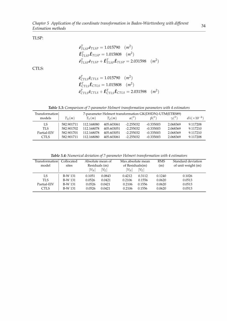
TLSP:
eTTLSP eTLSP = 1.015790 (m2)
ETTLSPETLSP = 1.015808 (m2)
eTTLSP eTLSP + ET
TLSPETLSP = 2.031598 (m2)
CTLS:
eTCTLS eCTLS = 1.015790 (m2)
ETCTLSECTLS = 1.015808 (m2)
eTCTLS eCTLS + ET
CTLSECTLS = 2.031598 (m2)
Table 5.3: Comparison of 7-parameter Helmert transformation parameters with 4 estimators
Transformation 7-parameter Helmert transformation GK(DHDN)-UTM(ETRS89)models TX(m) TY(m) TZ(m) α(′′) β(′′) γ(′′) dλ(×10−6)
LS 582.901711 112.168080 405.603061 -2.255032 -0.335003 2.068369 9.117208TLS 582.901702 112.168078 405.603051 -2.255032 -0.335003 2.068369 9.117210
Partial-EIV 582.901701 112.168078 405.603051 -2.255032 -0.335003 2.068369 9.117210CTLS 582.901711 112.168080 405.603061 -2.255032 -0.335003 2.068369 9.117208
Table 5.4: Numerical deviation of 7-parameter Helmert transformation with 4 estimatorsTransformation
modelCollocated
sitesAbsolute mean of
Residuals (m)Max.absolute mean
of Residuals(m)RMS(m)
Standard deviationof unit weight (m)
[VN ] [VE] [VN ] [VE]
LS B-W 131 0.1051 0.0843 0.4212 0.3112 0.1240 0.1026TLS B-W 131 0.0526 0.0421 0.2106 0.1556 0.0620 0.0513
Partial-EIV B-W 131 0.0526 0.0421 0.2106 0.1556 0.0620 0.0513CTLS B-W 131 0.0526 0.0421 0.2106 0.1556 0.0620 0.0513
Chapter 5 Application of the coordinate transformation in Baden-Württenberg with differentEstimation methods 35
Figure 5.7: Horizontal residuals after 7-parameter Helmert transformation in Baden-Württemberg network
Figure 5.8: Horizontal residuals after 7-parameter Helmert transformation in Baden-Württemberg network

Chapter 5 Application of the coordinate transformation in Baden-Württenberg with differentEstimation methods 36
Figure 5.9: Horizontal residuals after 7-parameter Helmert transformation in Baden-Württemberg network
Figure 5.10: Horizontal residuals after 7-parameter Helmert transformation in Baden-Württemberg network
Chapter 5 Application of the coordinate transformation in Baden-Württenberg with differentEstimation methods 37
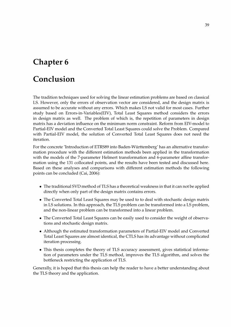
From the results above, we can see that, the same with 2D coordinate transformation, the SVD,Partial-EIV and CTLS all have better estimations than the LS. However,it is important to notehere, that the quadratics sums of the residuals of SVD, Partial-EIV and CTLS are the same witheach other. As a matter of fact the differences of them exist after 7 decimal places, which is nomeaning to discuss about it. So why they have almost the same residuals.After study into the transformation models, it is found that, unlike the design matrix in affinetransformation model, the elements by Helmert transformation in design matrix are calculated3 times. However, the weights and influences of these elements are different with that in affinetransformation. To be more specific we can see from the base transformation models and partof the residuals of the design matrix.
E
N1...
NnE1...
En
= E
H1 R1 0 0...
......
...Hn Rn 0 00 0 H1 R1...
......
...0 0 Hn Rn
ξ11ξ21ξ12ξ22
E
xg1...
xgnyg1
...ygnzg1
...zgn
=: E
0 −zl1 yl1 xl1...
......
...0 −zln yln xln
zl1 0 −xl1 yl1...
......
...zln 0 −xln yln−yl1 xl1 0 zl1
......
......
−yln xln 0 zln
δαδβδγλ
In the affine transformation, the transformation parameters after centering are ξ11, ξ12, ξ21 andξ22. The correspond data are λHcosα,−λRsinβ,λHsinα and λRcosβ, in which the rotation pa-rameters α and β are really small. So λHcosα and λRcosβ (ξ11,ξ22)have much bigger influenceson the design matrix. And after the calculate by SVD method, the absolute value of the first andfourth column of the residuals by design matrix are much bigger than second and third column.In the Helmert transformation, the transformation parameters after centering are δα,δβ,δγ andλ. The rotation parameters are very small too and the scale has relative bigger influence. Soafter the calculate by SVD method, the absolute value of the fourth column of the residuals bydesign matrix are much bigger than others.

Chapter 5 Application of the coordinate transformation in Baden-Württenberg with differentEstimation methods 38
Table 5.5: First 10 rows of the residuals by design matrix with 2D affine transformation
0.033378 3.179106×10⁻⁸ 2.6760356×10⁻⁸ 0.033378
0.068186 6.494339×10⁻⁸ 5.466658×10⁻⁸ 0.068186
-0.096281 -9.170245×10⁻⁸ -7.719122×10⁻⁸ -0.096281
0.005882 5.601823×10⁻⁹ 4.715376×10⁻⁹ 0.005882
0.040717 3.878038×10⁻⁸ 3.264367×10⁻⁸ 0.040717
0.041302 3.933744×10⁻⁸ 3.311258×10⁻⁸ 0.041302
-0.109623 -1.044095×10⁻⁷ -8.788746×10⁻⁸ -0.109623
-0.031937 -3.041849×10⁻⁸ -2.560499×10⁻⁸ -0.031937
-0.029446 -2.804580×10⁻⁸ -2.360776×10⁻⁸ -0.029446
0.001235 1.175897×10⁻⁹ 9.898197×10⁻¹⁰ 0.001235
Table 5.6: First 10 rows of the residuals by design matrix with 3D Helmert transformation
2.261038×10⁻⁷ 3.358953×10⁻⁸ -2.073878×10⁻⁷ -0.020682
5.867438×10⁻⁷ 8.716551×10⁻⁸ -5.381755×10⁻⁸ -0.053669
-9.169869×10⁻⁷ -1.362258×10⁻⁷ 8.410823×10⁻⁷ 0.083876
1.253344×10⁻⁷ 1.861943×10⁻⁸ -1.149597×10⁻⁷ -0.011464
4.069860×10⁻⁷ 6.046104×10⁻⁸ -3.732973×10⁻⁷ -0.037227
3.329597×10⁻⁷ 4.946384×10⁻⁷ -3.053987×10⁻⁷ -0.030456
-8.796520×10⁻⁷ -1.306794×10⁻⁷ 8.068378×10⁻⁷ 0.080461
-1.221220×10⁻⁷ -1.814221×10⁻⁸ 1.120133×10⁻⁷ 0.011170
-2.906775×10⁻⁷ -4.318247×10⁻⁸ 2.666163×10⁻⁷ 0.026588
3.301255×10⁻⁷ 4.904279×10⁻⁹ -3.027990×10⁻⁸ -0.003020
From the table we can see that, in the 3D Helmert transformation, there is only one columnin the residuals of design matrix has effective data. Which means in this case, although thecoordinates in design matrix have been calculated 3 times, 2 of them have very small residuals.Only one, the fourth column has effectively calculated. As a result, the final quadratics sumsof the residuals of SVD are almost the same with Partial-EIV and CTLS. But it can not provethat, SVD is as good as Partial-EIV and CTLS. Because it still has some systematical problems,like it has the residuals for 0. We could see that, SVD might be acceptable in 3D Helmerttransformation.
39
Chapter 6
Conclusion
The tradition techniques used for solving the linear estimation problems are based on classicalLS. However, only the errors of observation vector are considered, and the design matrix isassumed to be accurate without any errors. Which makes LS not valid for most cases. Furtherstudy based on Errors-in-Variables(EIV), Total Least Squares method considers the errorsin design matrix as well. The problem of which is, the repetition of parameters in designmatrix has a deviation influence on the minimum norm constraint. Reform from EIV-model toPartial-EIV model and the Converted Total Least Squares could solve the Problem. Comparedwith Partial-EIV model, the solution of Converted Total Least Squares does not need theiteration.
For the concrete ’Introduction of ETRS89 into Baden-Württemberg’ has an alternative transfor-mation procedure with the different estimation methods been applied in the transformationwith the models of the 7-parameter Helmert transformation and 6-parameter affine transfor-mation using the 131 collocated points, and the results have been tested and discussed here.Based on these analyses and comparisons with different estimation methods the followingpoints can be concluded (Cai, 2006):
• The traditional SVD method of TLS has a theoretical weakness in that it can not be applieddirectly when only part of the design matrix contains errors.
• The Converted Total Least Squares may be used to to deal with stochastic design matrixin LS solutions. In this approach, the TLS problem can be transformed into a LS problem,and the non-linear problem can be transformed into a linear problem.
• The Converted Total Least Squares can be easily used to consider the weight of observa-tions and stochastic design matrix.
• Although the estimated transformation parameters of Partial-EIV model and ConvertedTotal Least Squares are almost identical, the CTLS has its advantage without complicatediteration processing.
• This thesis completes the theory of TLS accuracy assessment, gives statistical informa-tion of parameters under the TLS method, improves the TLS algorithm, and solves thebottleneck restricting the application of TLS.
Generally, it is hoped that this thesis can help the reader to have a better understanding aboutthe TLS theory and the application.
X
Bibliography
Acar, M., Oezluedemir, M. T., Akzilmaz, O., Celik, R. N. and Ayan, T.(2006): Deformationanalysis with Total Least Squares, Istanbul Technical University, Division of Geodesy,Istanbul, Turkey.
Adcock, R. J. (1878): A problem in least squares. The Analyst, 5, 53-54.
Akyilmaz O (2007): Total Least-Squares Solution of Coordinate Transformation. SurveyReview.39(303):68-80
Badekas, J. (1969): Investigations related to the establishment of a world geodetic system, Re-port 124, Department of Geodetic Science, Ohio State University, Columbus.
Bursa, M. (1962): The theory of the determination of the non parallelism of the minor axis of thereference ellipsoid, polar axis of the Earth, and initial astronomical and geodetic merid-ians from observations of artificial Earth satellites. Studia Geophysica et Geodaetica 6,209-214.
Cai, J. (2000): The systematic analysis of the transformation between the German GeodeticReference System (DHDN, DHHN) and the ETRF System (DREF91). Earth Planets Space52, 947-952.
Cai, J. (2009): Systematical nalysis of the transformation between Gauss-Krüger-Coordinate/DHDN and UTM-Coordinate/ETRS89 in Baden-Württemberg with different estimationmethods. IAG Symposium VOLUME 134, Hermann Drewes(ED), Geodetic ReferenceFrame 2009.
Cai, J. (2003): Gutachten zur ’Einführung von ETRS89 in Baden-Württemberg’. GeodätischesInstitut der Universität Stuttgart, Stuttgart 2003.
Ding K., Ou J. and Zhao C. (2007): Methods of the least-suqares orthogonal distance fitting.Science of Surveying and Maping.32(3)17-19(in Chinese)
Gleser, L. J. (1981): Estimation in a multivariate ’errors in variables’ regression model: Largesample results. Ann. Statist. 9, 24-44.
Golub, G. H. (1973): Some modified matrix eigenvalue problems. SIAM Rev. 15, 318-344.
Golub, G. H. and Van Loan, C. F. (1980): An Analysis of the total least squares problem. Siam J.Humer Anal. Vol 17, No.6., December 1980.
Grafarend, E. (2006): Linear and Nonlinear Models: Fixed Effects, Random Effects, and MixedModels. de Gruyter, Berlin; New York.
Guo, R. (2007): Systematical analysis of the transformation procedures in Baden-Württembergwith Least Squares and Total Least Squares methods. Geodätisches Institut der Univer-sität Stuttgart, Stuttgart 2007.
Chapter 6 Conclusion XI
Kong, J., Yao Y., and Wu, H (2010): Iterative Method For Total Least-Squares. Geomatics andinformation science of wuhan university, 35(6):711-714(in Chinese)
Koopmans, T. C. (1937): Linear Regression Analysis of Economic Time Series. De Erven F.Bohn, Haarlem, The Netherlands.
Levin, M. J. (1964): Estimation of a system pulse transfer function in the presence of noise. IEEETrans. Automat. Control 9, 229-235
Madansky, A. (1959): The fitting of straight lines when both variables are subject to error. J.Amer. Statist. Assoc. 54, 173-205.
Micheal, K., Mathias, A. (2007) A weighted total least-squares algorithm for fitting a straightline. Meas. Sci Technol.No.18:3438-3442
Molodensky, M., Eremeev, S. and Yurkina, V. F. (1960): Metody izucheniya vnesnego gravitat-sion nogopolya I figure Zemli. Tr. CNIIGAIK, Moscow, 131.
Mühlich, M. and Mester, R. (1999): Subspace methods and equilibration in computer vision.Submitted to Citeseer 2000. Institute for Applied Physics, J. W. Goethe-UniversitätFrankfurt, Frankfurt, Germany.
Pearson, K. (1901): On lines and planes of closest fit to points in space, Philos. Mag., 2, pp.559-572.
Qiu W, Tao B, YaoY, Wu Y, Huang H (2008): The Theory and Method of Surveying Data Pro-cessing. Wuhan: Wuhan University Press.(in Chiness)
Schaffrin, B. and Felus, Y. (2003): On Total Least-Squares adjustment with constraints, In Pro-ceedings to IUGG General Ass. Department of Civil and Environmental Engineeringand geodetic Science, The Ohio State Universtity, Columbus.
Schaffrin, B. and Felus, Y. (2008):Multivariate total least squares adjustment for empiricalaffine transformations. In: Xu, P., Liu, J: Sermanis A(eds) International association ofgeodesy symposia: VI Hotine-Marussi symposium on the theoretical and computationalGeodesy, 29 May-2 June 2006, Wuhan,China, vol 132. Springer, Berlin, pp 238-242
Schaffrin, B. (2003): A Note on Constrained Total Least-Squares Estimation, In ComputaionalStatistics and Data Analysis, eingereicht Okt 2003.
Schaffin, B. (2005): Generalizing the Total Least-Squares Estimation for Empirical CoordinateTransformation, lecture in Geodetic Inst. Stuttgart.
Strang, G. (1988): Linear Algebra and its Applications, 3rd edition, Harcourt Brace Jovanovich,San Diego, pp. 505.
Van Huffel, S. and Zha, H. (1993): The Total Least-Squares problem, in Handbook of Statistics:Computational Statistics, (Rao, C. R., ed.), vol. 9, North Holland Publishing Company,Amsterdam, The Netherlands, 1993, pp. 377-408.
Van Huffel, S. and Lemmerling, P. (2002): Total Least Squares and Errors-in-Variables Model-ing, Kluwer Academic Publishers, Netherlands.
Van Huffel, S. and Vandewalle, J. (1991): The Total Least Squares Problem Computational As-pects and Analysis, Society for Industrial and Applied Mathematics, Philadelphia.

Chapter 6 Conclusion XII
Veis, G. (1960): Geodetic uses of artifical satellites, Smithsonian Contributions to Astrophysics3, 95-161.
Wang, B., Jiancheng, Li. and Liu, Chao (2015):A robust weighted total least squares algorithmand its geodetic applications.
Wei, M. (1992): Algebraic relations between the total least-squares and least square problemswith more than one solution. Numer. Math. 62:123-148(in Chinese)
Wolf, H. (1963): Geometric connection and re-orientation of three-dimensional triangulationnets, Bulletin Geodesique, 68, 165-169.
Wolf, R. P. and Ghilani, D. C. (1997): Adjustment computations: statistics and least squares insurveying and GIS, Wiley, New York, 347.
York, D. (1966): Least squares fitting of a straight line. Canad. J. Phys. 44, 1079-1086.
Yu, J (1996): On the Solvability of the Total Least-Squares Problem. Journal of Nanjing NormalUniversity (Nature Science).19(1)13-16(in Chinese)
Zhang Q., Bao Z. and Jiao L. (1994): A Neural Network Approach to Total Least-SquanresProblem. Journal of China Institute of Communications.15(4): 79-85(in Chinese)