Keskustelualoitteita #54 Joensuun yliopisto, Taloustieteet

Subsidies to forestry

Yrjänä Tolonen

ISBN 978-952-219-093-2 ISSN 1795-7885

No 54

1

SUBSIDIES TO FORESTRY

Yrjänä Tolonen* Department of Economics and Business Administration

University of Joensuu

FEBRUARY 2008

Abstract I analyze effects of investment and production subsidies to forestry and forest owners. Subsidies lead to an increase in forest owners' consumption, wealth and welfare but also in their indebtedness. A model is applied where with exogenous wood price there is no transitional dynamics. However, if a forest owner’s supply affects wood price it is profitable for her to divide the subsidy- induced increase in forest reserves (and in wood production) over time. I also compare permanent and temporary subsidies. Keywords: dynamics of imperfect competition, input markets, renewable resources, forestry

* Author’s address: Department of Economics and Business Administration, University of Joensuu, P. O.

Box 111 (Yliopistokatu 2), FI-80101 Joensuu, Finland email: yrjana.tolonen@joensuu.fi

2

1. INTRODUCTION

Sixty-five per cent of the Finnish wood-producing forests are owned by private persons. To these owners the public sector gives, since the 1960s, aid, the purpose of which is to increase the long-term cutting potential of the forests. Especially subsidized are artificial regeneration, draining, fertilizing and forest roads building (see Linden and Leppänen (2004)) The size of this aid is considerable. For example, in financing of silvicultural and forest improvement works in private forests, the public subsidy was in the 1990s between 50 to 70 per cent of the private outlays (see METLA (2003)). This paper analyzes forestry subsidies. I differentiate between investment and production subsidies. In practice, three types of forestry investments are distinguished. First, there is reforesting bare lands like cornfields. For northern tree types the growing period is more than thirty (maybe one hundred) years. On the other hand, with other tree types like eucalyptus in South- American countries the situation is different. One can (and does) speak about tree- fields and the investing means creating new tree- fields. Second, there are improvement works of existing forests like draining, forest road building etc. The characteristic feature of these two types is that they may be considered permanent. I mean these when I speak about forest investments and the expression “increase in effective forest reserves” is intended to cover both an increase in area and in quality of forests. Third, many times in (Nordic) literature the costs of replanting the cut areas are included in investments. This may be defended by the long maturity period. Theoretically, as will be discussed below, a continuous replanting is considered optimal. In addition, replanting is often mandatory, for example, because of environmental reasons. With tree types with a considerably shorter maturity replanting may be characterized as sowing on existing tree fields. I include these costs in production costs. Into production costs I also include, naturally, cutting trees and transporting them. In Finland, the main demand for wood comes from a few large firms producing paper products There are accusations about their collusion in buying wood. On the other hand, private Finnish forest owners are well-organized via their associations. Recently, paper industry has accused forest owners for collusion in wood selling (see HS (2008)). All this seems to imply a non-competitive wood market. There are,

3

however, factors pointing to a more competitive situation. About one-third of Finnish wood consumption is imported from Russia at competitive prices. At first sight, it would seem that this implies lower (and more competitive) wood prices to Finnish forest owners. This is not necessarily so. A considerable part of these imports consist of such wood (birch etc.) which does not grow plentifully in Finland but is needed as a component part in the optimal mixture for producing final goods like paper. In this way, these imports can lead to increased demand for ordinary Finnish wood like spruce and pine and to an increase in their price and strengthen a potential monopoly position of Finnish forest-owners. I have modeled wood markets as follows. The wood buyers, that is, the producers of final goods based on wood, are competitive. The wood sellers (the forest owners) are modeled in two ways. In a competitive situation wood prices are exogenous to forest owners while in a non-competitive situation these owners take into account the effect of their supply on wood price. This I have formulated in a rather general way. For the analysis we first need a description of the output of forest reserves. A venerable model is Faustmann (1849). It is still considered to be theoretically valid (see, e.g., Samuelson (1976)). It is a profit maximization model where harvesting is related to stands with different ages and there is replanting. Based on this, Mitra and Wan (1985) showed that the following (stationary) forest is optimal: A forest is split into M equal subplots each containing trees of age a (a = 0,1,...,M-1). In each period, trees of age M are cut down and the subplot so cleared is planted with seedlings (age zero trees.) I will apply a continuous-time modification of this and analyze a situation where there are subplots of every age on a continuous time scale and cutting (and replanting) takes place continuously. I will assume that investments contribute instantaneously to larger production of wood. This simplifies the analysis considerably. In forestry investments there are obvious congestion phenomena. When foresting new areas, the best sites are taken into cultivation first and less productive sites later on. Or the most effective roads are built

4

first. I model this as installment costs which grow with the cumulative investments. These investments lead to an increase in the effective size of forests which I will call reserves. Other outlays like cutting and transporting wood or planting in the cut areas, are included in variable costs. Two types of subsidies are discussed. The first is investment subsidy. By it I mean support to outlays which increase reserves. The second is production subsidy which reduces variable costs of forest owner. When comparing permanent subsidies, it turns out that their consequences are surprisingly similar. However, if subsidies are temporary, their effects may differ rather much. I apply a dynamic Ramsey-type model. It has similarities to those presented, e.g., by Blanchard and Fischer (1989, Ch.2.4.) or Sen and Turnovsky (1991). In their models transitional dynamics is generated by increasing investment installation costs in competitive circumstances with decreasing returns to scale technology. These installation costs increase when the size of investment flow increases. Without this there are no transitional dynamics. In my model, there are constant returns to scale and no such installation costs. In a competitive situation a subsidy leads to an instantaneous jump to a new steady state value. That there are installment costs which depend on cumulative investments does not change this. Surprisingly, it turns out that non-competitiveness among wood sellers is sufficient to generate transitional dynamics. Finance markets are assumed fully functioning. The forest-owner can lend and borrow at a given interest rate which is equal to her personal time preference rate. This contrasts with forestry models with various types of finance markets imperfections. For example, Tahvonen et al. (2001) and Brazee (2003) discuss, among other things, situations where forest owners pay higher interest rate as borrowers than as lenders. This leads to a so called Volvo- effect where consumption decisions determine harvesting time. Finally, Tahvonen and Salo (1999) discuss optimal forest rotation in a modified Ramsey- model with perfect capital markets. The modification concerns including the forest reserves in utility function as bequests. For utility, I will apply a conventional formulation. Abel (1982) showed that temporary investment subsidy is, in the short run, more expansionary than a permanent subsidy because the investor tries to have the subsidy benefit as long as it lasts in spite of

5

higher installment costs. Similar results were obtained by Sen and Turnovsky (1990) within an open-economy framework. This probably applies in my model also if there is transitional dynamics. On the other hand, as I show, a temporary production subsidy is less expansionary than a permanent one. Even a temporary production subsidy leads larger reserves but when considering their yield one has to take into consideration that the variable production costs increase after the subsidy stops. The model is presented in Section 2 which discusses forest owners’ optimization and the ensuing first order conditions for the two types of permanent subsidies in a competitive and non-competitive situations. Long run effects are presented in Section 3 and transitional dynamics in Section 4. Forest owners' indebtedness and wealth are discussed in Section 5. Section 6 deals with temporary subsidies and compares their effects with those of permanent subsidies. Concluding remarks are in Section 7.

2. THE MODEL

Wood is produced in forests owned by a representative consumer - forest owner - wood producer. The effective size of these forests is denoted by R which I will call (forest) reserves. These reserves contain different age groups of trees and are cut and replanted at a constant rate σ. Accordingly, there is a continuous flow of wood σR(t) where t denotes time. Variable unit costs (going to outsiders) of, for example, cutting and transporting wood are assumed constant. Without affecting the conclusions we can set them equal to zero. Investments, I, increase reserves and they are financed by borrowing and/or from retained earnings. There is no depreciation of reserves because all cut areas are replanted. Installation costs of investments increase with the

6

size of R. A simple formulation for this is to assume that the total costs of investing I is (1+h(R))I, h' > 0. The forest owner maximizes her intertemporal utility depending on her consumption c subject to the (flow) budget constraint. She may take loans from a fully functioning credit market at a constant interest rate i* and her subjective discount rate is equal to this. Her indebtedness at time t is B(t). For forest investments she may obtain an investment subsidy z measured as a share of the overall investment costs. Correspondingly, she may obtain unit production subsidy, s, for producing wood. All in all, her optimization may be presented as ∞

max ∫u(c(t))e- i*t

dt (1) 0 subject to dB/dt= i*B + c + (1-z)(1+h(R))I - wσR - sσR (2a) dR/dt = I (2b) where u denotes instantaneous utility, u’> 0, u’’< 0, and w denotes wood price. Wood market equilibrium may be presented as w = f(σR) = w(R). In the competitive situation wood price is exogenous to the forest owner, that is, w' = 0. In the non-competitive situation w' < 0, w'' < 0. An increase in a forest owner's wood supply leads to a decrease in its price. For forest owner’s optimization, the Hamiltonian is:

H = {u(c)- µ[ i*B+c+(1-z)(1+h(R))I–sσR-wσR]+µqI} e-i*t

(3)

The control variables are c and I while B and R are state variables. The

co- state variables are - µ(t)e-i*t

for debt accumulation and

µ(t)q(t)e-i*t

for reserve accumulation. The first degree optimum conditions are:

7

u’(c(t)) = µ(t) (from dH/dc = 0) (4a)

(1-z)(1+h(R)) = q (from dH/dI = 0 ) (4b)

d(-µe-i*t

)/dt = µi*e-i*t

(4c)

d [µqe-i*t

] /dt = µ[ -wσ - w'σR - sσ + (1-z) h'(R)I ] e-i*t

(4d) Additionally, there are transversality conditions which may be shown to be fulfilled. From Eq. (4c), dµ/dt = 0 or µ is constant. Because the utility function, u, is decreasingly increasing, we may conclude from Eq. (4a) that consumption is the same for all t, that is, there is a complete consumption smoothing. Accordingly, from Eqs. (2a) and (2b) c(t) = c* = (w*+s)σR* - i*B* (5) where asterisks refer to long run (steady state) values. Differentiating

Eq. (4b) with respect to q we may see that Rq > 0 and from this that

Iq > 0. Using dµ/dt = 0 and Eq. (4c) we obtain from Eq. (4d): dq/dt = i*q - wσ - w'σR - sσ

+ (1-z)h’(R)I (6)

8

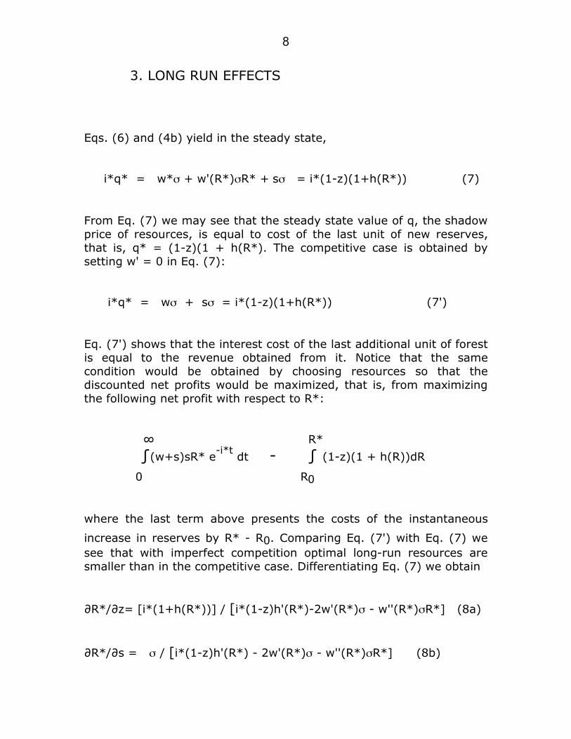
3. LONG RUN EFFECTS Eqs. (6) and (4b) yield in the steady state, i*q* = w*σ + w'(R*)σR* +

sσ

= i*(1-z)(1+h(R*)) (7)

From Eq. (7) we may see that the steady state value of q, the shadow price of resources, is equal to cost of the last unit of new reserves, that is, q* = (1-z)(1 + h(R*). The competitive case is obtained by setting w' = 0 in Eq. (7): i*q* = wσ + sσ

= i*(1-z)(1+h(R*)) (7')

Eq. (7') shows that the interest cost of the last additional unit of forest is equal to the revenue obtained from it. Notice that the same condition would be obtained by choosing resources so that the discounted net profits would be maximized, that is, from maximizing the following net profit with respect to R*: ∞ R*

∫(w+s)sR* e-i*t

dt - ∫ (1-z)(1 + h(R))dR

0 R0 where the last term above presents the costs of the instantaneous

increase in reserves by R* - R0. Comparing Eq. (7') with Eq. (7) we see that with imperfect competition optimal long-run resources are smaller than in the competitive case. Differentiating Eq. (7) we obtain ∂R*/∂z= [i*(1+h(R*))] / [i*(1-z)h'(R*)-2w'(R*)σ - w''(R*)σR*] (8a) ∂R*/∂s = σ / [i*(1-z)h'(R*) - 2w'(R*)σ - w''(R*)σR*] (8b)

9

which are positive because w',w'' ≤ 0 and h' > 0. Both types of subsidies lead to larger steady state reserves both in the non-competitive and competitive case. 4. SYSTEM DYNAMICS The system may be seen as functions of two variables, R and q. Linearizing the non-linear functions in Equations (2b) and (6) around the steady state values, denoted by asterisks, yields dR/dt = Iq(q*)(q-q*) (9a) dq/dt = i*q - sσ - w*σ - w'(R*)σR*- [2w'(R*)σ+ w''(R*)σR*][R-R*] +(1-z)Iq(q*)h'(R*)[q-q*] (9b) These equations may be presented in matrix form as: dR/dt 0 Iq(q*) R constant | | = | | | | + | | (10) dq/dt E G q constant where E = - [2w'(R*)σ + w''(R*)σR*] > 0 and G = i* + (1-z)Iqh'(R*) > 0. When solving these two simultaneous differential equations, one of the characteristic roots is negative, equal to

v = [G-(G2+4IqE)

1/2]/2, and the other is positive, equal to

10

[G+(G2+4IqE)

1/2]/2. Consequently, we have saddle-path dynamics.

Notice that in the competitive situation E = 0 which implies that the stable root v is zero and, accordingly, that there are no transitional dynamics. Reserves jump instantaneously to the steady state level. The optimal path is the stable branch of the saddle-paths. A particular solution of these simultaneous differential equations is, applying Eq. (7) in Eq. (9b), q(t) = q* , R(t) = R* and so we obtain the time path of R as:

R(t) = R* + (R0 - R*)evt

(11)

where R0 is the initial reserves. Eq. (11) shows the gradual growth of reserves to their new steady state size as a consequence of subsidy. As Eq. (3) shows, the wood price starts falling according to the increase in forest reserves. Differentiating Eq. (11) and inserting it into Eq. (9a) yields the corresponding optimal path for q:

q(t) = q* + (v/Iq)(R0 - R*)evt

= q* + (v/Iq)(R(t) - R*) (12) A conclusion from Eq. 12) is that in the competitive case the shadow price of resources q adjusts instantaneously to its steady state level.

11

5. DEBT AND WEALTH Using Eqs. (4b), (5), (7), (11) and (12) in Eq. (2a) and linearizing we obtain the following first-order differential equation for indebtedness (see Appendix):

dB/dt = i*B - i*B* + (q*v - i*q*)(R0 - R*)evt

(13) Solving this yields

B(t) = B* + Ω [ R0 – R*] evt

= B* + Ω [ R(t) – R*] (14) where Ω = q* = 1+h(R*) > 1 and B* is the steady state indebtedness. We may see from Eq. (14) that the forest owner's debt increases in the same way as the reserves increase. Further, from Eq. (14), ∂B*/∂z = Ω [∂R*/∂z] (15a) ∂B*/∂s = Ω [∂R*/∂s] (15b) As may be seen, the long-run indebtedness of the forest owner increases as a consequence of both types of subsidies. Applying this in Eq. (14) and using Eq. (11) we may infer that debt increases along its time path in the non-competitive case. The competitive case is straightforward: reserves increase instantaneously to the long-run level. As is obvious this is entirely financed by increased debt.

From Eq. (14), B* - B(0) = Ω [ R* – R0] where Ω > 1. This should not be interpreted so that the wealth of the forest-owner decreases in the long run as a consequence of subsidies. Instead, we should compare debt with the value of reserves. This value V is the present (discounted) value of sales revenues at time 0 or

12

∞

V = ∫ (w(t) + s)σR(t)e -i*t

dt (16) 0 As an example let us analyze the competitive case. As discussed above, subsidies (or an increase in subsidies) lead to an instantaneous

increase in reserves, let us say from R1* to R2*. Assume for simplicity that there are no subsidies in the initial situation which is denoted by

subscript 1. The (post-subsidy) value of reserves R2* at wood price w is, from (16) applying Eq. (7'), ∞

V2 = ∫ (w+s)σR2*e -i*t

dt 0

= (w+s)σR2*/i* = (1-z)(1+h(R2*))R2*

Correspondingly, the value of reserves R1* at price w is ∞

V1 = ∫ wσR1*e -i*t

dt = wσR1*/i* = (1+h(R1*))R1* 0 As may be shown t

he cost of the instantaneous reserves increase from R1* to R2* is

R2*

C = ∫ (1-z)(1 + h(R))dR = (1-z)(1+h(ξ))(R2*- R1*)

R1*

where R1* < ξ < R2*. Because there is no transitional dynamics this

is equal to the (instantaneous) debt increase B2* - B1*. The increase

13

in income flow, (w+s)σR2* - wσR1*, is used for the increase in interest payments and in consumption. Let us analyze the two types of subsidy separately. If there is production subsidy in state 2, the (potential)

increase in net wealth, V2 - V1 - C, is

(1+h(R2*))R2* - (1+h(R1*))R1* = (1+h(ξ))(R2* - R1*)

= [h(R2*) - h(ξ)] R2* + [(h(ξ) - h(R1*)]R1*

This is positive because h is an increasing function and R1* < ξ <

R2*. Production subsidy increases the forest owner's net wealth. For investment subsidy, the increase in net wealth may be presented as

wσR2*/i* - wσR1*/i* - (1-z)(1+h(ξ))(R2*- R1*)

= (wσ/i*)(R2*- R1*) - (1-z)(1+h(ξ))(R2*- R1*)

= (1-z)(1+h(R2*))(R2*- R1*) - (1-z)(1+h(ξ))(R2*- R1*)

= (1-z) [h(R2*) - h(ξ)](R2*- R1*)

This is positive because ξ < R2. Investment subsidy increases the forest-owner's net wealth.

14

6. TEMPORARY SUBSIDIES In the competitive situation, the forest-owner obviously reaches highest welfare by maximizing her discounted net profits because there is no transitional dynamics of reserves (cf. the discussion in Section 3). Assume that production subsidy is paid from time 0 to time T. The forest-owner chooses the reserves R* so that the following is maximized: T ∞

∫ [wσR*+sσR*] e-i*t

dt + ∫ wσR*e-i*t

dt 0 T

R* (17)

- (1-z)∫ (1+h(R))dR

R0

where R0 is the initial level of reserves and R* denotes their post-subsidy steady-state levels. The first order condition is

wσ + (1 – e-i*T

)sσ = (1-z) i*(1+ h(R*)) (18) Because h is an increasing function of R, Eq. (18) shows that a temporary production subsidy leads to an increase in reserves which is smaller than with permanent subsidy. Eq. (18) may be interpreted so that the average income from selling one unit of wood must equal the interest cost of the last unit invested and this average income is smaller with temporary subsidy. When the owner invests she has to take into account that her costs increase after time T. As is obvious for investment subsidy, temporariness does not affect the results at all. How about temporary subsidies in the non-competitive situation? There are now transitional dynamics caused by falling price. Referring

15

to Abel (1982) we may expect that temporary forest investment subsidy speeds up the increase in investment as compared with permanent subsidy as long as the marginal benefit from subsidy more than offsets the fall in wood price. The long run effect is smaller reserves than with permanent subsidy because a larger short-run investment leads to an earlier price fall. Opposite to this, for production subsidy the increase in investments is smaller for temporary subsidy than for permanent one. After all, so this is the case if wood price does not fall. To show the effects of temporary subsidies rigorously is complicated and I leave it at these remarks 7. CONCLUSIONS AND CONCLUDING REMARKS Both an investment subsidy and a production subsidy lead to an increase in forest reserves and wood production. All or a part of this is financed by increased indebtedness. The forest- owners' net wealth, consumption and welfare increase. For production subsidy, these increases are smaller for a temporary subsidy than for a permanent subsidy. For investment subsidy the increases are either equal or larger for a temporary subsidy. Transitional dynamics is created by non-competitiveness and the long run reserves are smaller (for a further analysis, see Tolonen (2008)). Assume now that the representative agent represents one among a large group of (identical) consumer- owners and her personal wood supply does not affect wood price even if all agents' combined supply does. Obviously here investment subsidies lead to too large and too rapid investments (from the forest owners' point of view).

16

REFERENCES: Abel,A, 1982. Dynamic effects of permanent and temporary tax policies in a q model of investment. Journal of Monetary Economics 9, 353-373. Brazee, R.J., 2003. The Volvo theorem: From myth to behavior model. In: Helles,F. et al. (Eds.). Recent Accomplishments in Applied Forest Economics Research, Kluwer Academic Publishers, pp.39-48. Faustmann, M., 1849. Berechnung des Wertes welchen Waldboden sowie noch nicht haubare Holzbestände fur die Weltwirtschaft besitzen. Allgemeine Wald und Jagd Zeitung 15, 441-455. Linden,M. and J.Leppänen, 2004. Effects of public financed aid on private forest investments: some evidence from Finland 1963-2000. Forthcoming in Scandinavian Journal of Forest Research. Lucas,R.E., 1967. Adjustment costs and the theory of supply. Journal of Political Economy 75, 321-334. Hayashi,F., 1982. Tobin's q rational expectations, and optimal investment rule. Econometrica 50,213-224. HS (Helsingin Sanomat), 2008. Metsäteollisuus haluaa myös puun myyjät markkinaoikeuteen. January 23, 2008. METLA (Finnish Forest Research Insitute) , 2003. Finnish forest sector outlook 2003-2004. Mita,T. and H.Y.Wan, 1985. Some theoretical results on the economics of forestry. Review of Economic Studies LII, 263-282. Samuelson, P., 1976. Economics of forestry in an evolving society. Economic Inquiry XIV, 466-491. Sen,P. and S.J.Turnovsky, 1990. Investment tax credit in an open economy. Journal of Public Economics 42, 277-299. Sen,P. and S.J.Turnovsky, 1991. Fiscal policy, capital accumulation and debt in an open economy. Oxford Economic Papers 43, 001-024.

17

Tahvonen,O. and S.Salo, 1999. Optimal forest rotation with in situ preferences. Journal of Environmental Economics and Management 37, 106-128. Tahvonen,O.,S.Salo and J.Kuuluvainen, 2001. Optimal forest rotation under borrowing constraint. Journal Of Economics and Control 25, 1595-1627. Tolonen,Y., 2008. Imperfect competition in input good market: a dynamic analysis. Discussion Papers (Economics) 53, University of Joensuu, Finland

18

APPENDIX SEC. 2. Transversality conditions are fulfilled Optimality requires the following transversality conditions: lim H = 0 t→∞

lim -µe-i*t

= 0 t→∞

lim µq e- i*t

= 0 t→∞

H = { u(c)- µ [ i*B + c + (1-z)(1+h(R))I – sσR - w(R)σR ]+µqI } e-i*t

Because µ and c are constant and I* = 0, the conditions are fulfilled if

lim Re- i*t

= 0 t→∞

lim B e- i*t

= 0 t→∞

lim q e- i*t

= 0 t→∞ Because R*, B* and q* are finite the conditions are fulfilled.

19

SEC. 2 AND 4: From Eq. (4c)

d(-µe-i*t

)/dt = [d(-µ)/dt] e-i*t

+ µi*ei*t

= - (∂H/∂B) = µi*ei*t

From this, dµ/dt = 0. Applying this, the fourth condition becomes

d [µqe-i*t

] /dt = µe-i*t

(dq/dt) + q d(µe-i*t

)/dt

= µe-i*t

(dq/dt) - qi*µe-i*t

= - (∂H/∂R) )

= µ [- wσ - w'σR - sσ + (1-z)h'(R)I]e-i*t

Dividing by µe-i*t

yields dq/dt = i*q - wσ - w'σR - sσ

+ (1-z)h'(R)I

Linearizing, dq/dt = i*q - w*σ - w'(R*)σR* =

- [2w'(R*)σ + w''(R*)σR*][R-R*] + (1-z)Iq(q*)h'(R*)[q-q*]

+(1-z) I* h’(R*) + (1-z)Iq(q*)h'(R*) [q-q*] + (1-z)I*h''(R*)[R-R*] - sσ Because I* = 0 these are as presented in text.Linearizing Eq. (2b) yields dR/dt = I(q*) + Iq(q-q*) = Iq(q*)(q-q*)

20

SEC.5. Foreign debt dB/dt = c + i*B - wσR + (1+h(R))I (use Eq. (5)) = w*σ R*- i*B*+sσR* + i*B - wσR - sσR + (1-z) (1+h(R))I (use Eq.(4b)) = i*B - i*B* + (w*+s)σR* - (w+s)σR + qI (linearize) = i*B - i*B* + (w*+s)σR* - (w*+s)σR* - [w*σ + w'(R*)σR*+sσ](R(t) – R*) + q*Iq (q-q*) (use Eq. (11) and Eq. (12))

= i*B - i*B* - [w*σ + w'(R*)σR*+ sσ](R0 - R*)evt

+ q*v (R0 - R*)evt

= i*B - i*B* - i*q*(R0 - R*)evt

+ q*v (R0 - R*)evt

(when using (7))

Solving this first-degree differential equation yields

B(t) = Mei*t

+ ei*t ∫[ – i*B*] e

-i*t dt

+ ei*t ∫[- i*q*

+ q*v][R0 – R*] e

-i*t + vt dt

= Mei*t

+ B* + [-i*q* + q*v][1/(v – i*)]

[ R0 – R*] e

vt

= Mei*t

+ B* + Ω[ R0 – R*] evt

21

where, using Eq. (7), Ω = q* = 1+h(R*). To obtain M set t = 0: M

= B(0) – B* - Ω [R0 – R*]. Inserting this into the equation above and

dividing by ei*t

yields

B(t)e–i*t

= B(0) – B* - Ω [R0 – R*]

+ B* e-i*t

+ Ω [R0 – R*] evt-i*t

Letting t approach infinity and applying the transversality conditions yields

0 = B(0) – B* - Ω[ R0 – R*] = M

Inserting this into the solution of the first order differential equation yields

B(t) = B* + Ω[ R0 – R*] evt

.

Overall investment cost: Costs of investing R* – R are

(Rs – Rs-1)(1+hs) + (Rs-1 – Rs-2)(1+hs-1) + ….. Letting the division approach zero this is R*

∫ (1 + h(R))dR = (1+h(ξ))(R*-R0), R0 < ξ < R*

R0 by intermediate theorem of integral calculus.