symmetry and bifurcations of momentum mappings*marsden/bib/1981/01-armamo1981/armamo19… ·...
TRANSCRIPT
Communications inCommun. Math. Phys. 78, 455-478 (1981) MathθΓΠatiCΘl
Physics© Springer-Verlag 1981
Symmetry and Bifurcations of Momentum Mappings*
Judith M. Arms1, Jerrold E. Marsden2, and Vincent Moncrief3
1 Department of Mathematics, University of Washington, Seattle, WA 98195, USA2 Department of Mathematics, University of California, Berkeley, CA 94720, USA3 Department of Physics, Yale University, P.O. Box 2014 Yale Station, New Haven, CT 06520, USA
Abstract. The zero set of a momentum mapping is shown to have a singularityat each point with symmetry. The zero set is diffeomorphic to the product of amanifold and the zero set of a homogeneous quadratic function. The proof usesthe Kuranishi theory of deformations. Among the applications, it is shown thatthe set of all solutions of the Yang-Mills equations on a Lorentz manifold has asingularity at any solution with symmetry, in the sense of a pure gaugesymmetry. Similarly, the set of solutions of Einstein's equations has asingularity at any solution that has spacelike Killing fields, provided thespacetime has a compact Cauchy surface.
1. Introduction
A momentum mapping is the conserved quantity associated with a symmetrygroup acting on phase space. The purpose of this paper is to study the level sets ofa momentum mapping and, especially, the zero set. The main results of the papershow that these level sets have cone-type singularities at any point (in phase space)which itself has some symmetries.
Level sets of momentum mappings are important in several contexts.
a) The Topology of Hamiltonian Systems with Symmetry
The momentum mapping is conserved by a given Hamiltonian system withsymmetry, so knowledge of the level sets and their bifurcations can help inunderstanding the qualitative features of its flow, as has been emphasized by Smale(1970). In this context, one can reduce a Hamiltonian system with symmetry,looking at the orbit space of a level set of the momentum mapping. This general
* This work was partially supported by the National Science Foundation. The second author wassupported by a Killam Visiting fellowship at the University of Calgary during the completion of thepaper
0010-3616/81/0078/0455/$04.80

456 J. M. Arms, J. E. Marsden, and V. Moncrief
procedure, due to Marsden and Weinstein (1974) generalizes the classical elim-ination of 2k variables when k integrals in involution are known as well as Jacobi'selimination of the node in celestial mechanics.
b) Constraints in Classical Relativistic Field Theories
Under certain general conditions, the constraints in Lagrangian field theories canbe phrased as saying that an appropriate momentum mapping vanish (see Gotayet al., 1980). This idea first arose in general relativity and (classical Lorentzian)gauge theory. The present paper grew out of our work in general relativity (Fischeret al., 1980) and gauge theory (Arms, 1980). The study of the space of all solutionsto a classical relativistic field theory is thus closely related to the study of the zeroset of an associated momentum mapping1. This space of classical solutions plays akey role in perturbation theory about a given solution. If this solution is a point ofsymmetry for the gauge group generating the constraints, then first orderperturbation theory must be supplemented by second order conditions in order toapproximate solutions to the nonlinear equations.
Most of the work on classical field theory assumes that the space ofsolutions forms a manifold, or has restricted attention to points where thatassumption holds. This is true, for example, in Marsden and Weinstein (1974), inthe work of Gotay et al. (1978) on the Dirac theory of constraints, in Segal (1978)on Yang-Mills theory and in most perturbation work in field theory. In generalrelativity however, Brill and Deser (1973) questioned this assumption, and foundthat it sometimes fails. In fact it fails exactly when there is symmetry, i.e. exactly inthe cases of interest, for the known solutions which are perturbed are symmetric.Similar phenomena for more general situations in general relativity were obtainedin a series of papers of Choquet-Bruhat et al. see Fischer et al. (1980) andreferences therein. For gauge theories similar results are due to Moncrief (1977)and Arms (1979a, 1980).
c) Perturbative Quantum Theory
The breakdown of classical perturbation theory near a solution with symmetryhas a quantum analogue that arises if one quantizes the fluctuations about a givensymmetric classical background solution. Even at first order, the quantized form ofthe linearized constraints does not adequately capture the content of the nonlinearconstraints. Using the method of Dirac, one must restrict the linearized constraintsby certain second order quantum constraints in order to exclude some physicallyspurious quantum states. An example was worked out by Moncrief (1978) it wasshown that without the second order conditions, states which violate thecorrespondence principle would be allowed.
A similar phenomenon will occur in the path integral quantization of smallfluctuations about a symmetric classical background. One would find it essentialto expand certain projections of the constraints (which appear in the classical
1 Our work applies to Lorentzian field theories. The results for Euclidean field theories, such asYang-Mills fields on S4 or gravitational instantons are different; see Atiyah et al. (1978)
Bifurcations of Momentum Mappings 457
action integral) to higher than linear order to accurately approximate theircontribution to the quantum theory.
This paper describes the structure of the singularities in the zero sets ofmomentum mappings that occur at points of symmetry when the group giving riseto the momentum mapping is compact or admits a local slice. We emphasize zerolevels rather than general level sets both for simplicity and because this coversmost of the examples of interest. In perturbation theory, it is assumed that thelinearized equations in a field theory such as relativity are a good approximationto the original nonlinear equation i.e., the solution set of the nonlinear equationswhen linearized, is diffeomorphic to the solution set of the linearized equations. Inthis paper we show that at points with symmetries the nonlinear zero set isdiffeomorphic to the zero set of a homogeneous quadratic form given by thesecond order perturbation equations. Moreover, this zero set is the product of amanifold of solutions with the same degree of symmetry and a cone of solutions forwhich one or more of the symmetries has been broken. An important consequencefor perturbation theory is that while second order conditions must be imposed onthe first order perturbations, there are no additional higher order obstructions tocompleting the perturbation expansion.
The method of proof involves a function borrowed, via the work of Atiyah etal. (1978) on gauge theory, from the Kuranishi Theorem on deformation ofcomplex structures. However, the proof itself makes no reference to that work.What is directly and extensively used is the machinery of groups of symplectomor-phisms (canonical transformations) acting on a symplectic manifold (phase space)which has an additional metric structure. The relevant machinery is reviewed inSect. 2 for a more leisurely discussion, see Chaps. 3 and 4 of Abraham andMarsden (1978). The main results of the paper are contained in Theorems 1-5 inSects. 3-6. Section 7 resumes the present discussion and Sect. 8 gives some specificexamples.
The critical or bifurcation points that occur are proved to be non-degenerate ina suitable sense (see Theorem 2), so it may be possible to develop a correspondingglobal Morse theory. [Local Morse theory does in fact appear in the precedingwork by Fischer et al. (1979), but those methods are not pursued here.] Thepresent paper deals only with the local structure of the singularities.
2. Background and Notation
We recall some concepts and list the notations that will be used throughout thepaper. We let (P, ω) be a given symplectic manifold (possibly infinite dimensionalin which case ω is only required to be a weak symplectic form). Let G be a Liegroup with Lie algebra g. Assume G acts symplectically on P the action is denotedby (g,x)t-*g x = Φg(x). Let
be an Ad*-equivariant momentum mapping. This means two things. First, Jsatisfies the identity
v,ξy=ωx(ξP(X\v), (1)
458 J. M. Arms, J. E. Marsden, and V. Moncrief
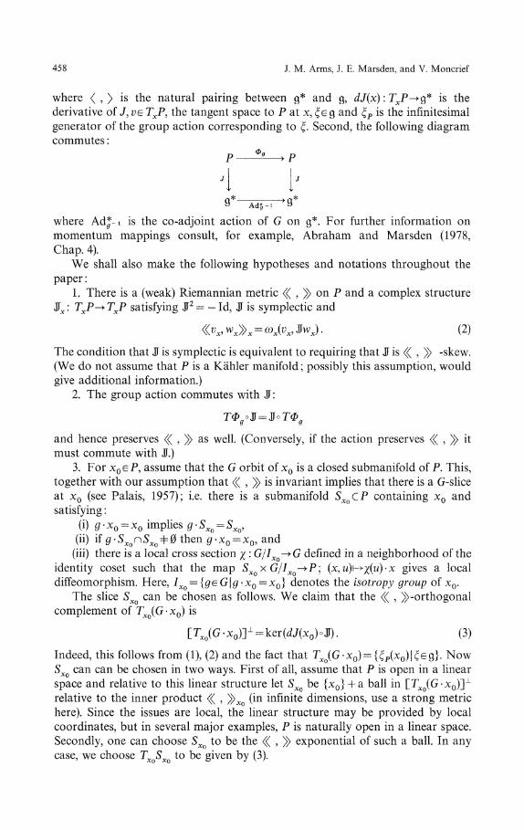
where < , > is the natural pairing between g* and g, dJ(x): TxP-»g* is thederivative of J, υe TXP, the tangent space to P at x, ξe g and ξp is the infinitesimalgenerator of the group action corresponding to ξ. Second, the following diagramcommutes:
p Φs > P
9* Ads-i '9*
where Ad*- 1 is the co-adjoint action of G on g*. For further information onmomentum mappings consult, for example, Abraham and Marsden (1978,Chap. 4).
We shall also make the following hypotheses and notations throughout thepaper :
1. There is a (weak) Riemannian metric <^ , ^> on P and a complex structure$x: TXP^TXP satisfying $2= -Id, JJ is symplectic and
«vx,wx»x = ωx(vxjwx). (2)
The condition that $ is symplectic is equivalent to requiring that Jί is « , » -skew.(We do not assume that P is a Kahler manifold possibly this assumption, wouldgive additional information.)
2. The group action commutes with Jί:
and hence preserves « , » as well. (Conversely, if the action preserves « , » itmust commute with Jί.)
3. For x0eP, assume that the G orbit of x0 is a closed submanifold of P. This,together with our assumption that « , » is invariant implies that there is a G-sliceat x0 (see Palais, 1957); i.e. there is a submanifold SXQCP containing x0 andsatisfying :
(i) g x0 = x0 implies g SXQ = SXQ,(ii) if g SXQnSXQ φ 0 then g-x0 = x0, and
(iii) there is a local cross section χ : G/IXQ-^G defined in a neighborhood of theidentity coset such that the map S X Q x G / I X Q - + P ; (x, u)t-*χ(u) x gives a localdiffeomorphism. Here, /Xo = {gfeG|gf x0 = x0} denotes the isotropy group of x0.
The slice SXQ can be chosen as follows. We claim that the « , » -orthogonalcomplement of TXQ(G - x0) is
[Γ:co(G-x0)]1 = ker(dJ(x0)oJ|). (3)
Indeed, this follows from (1), (2) and the fact that TXo(G x0) = { ξ P ( x 0 ) \ ξ £ $ } . NowSXQ can can be chosen in two ways. First of all, assume that P is open in a linearspace and relative to this linear structure let SXQ be {x0} + a ball in [jΓ^G Xo)]1
relative to the inner product <^ , ^>xo (in infinite dimensions, use a strong metrichere). Since the issues are local, the linear structure may be provided by localcoordinates, but in several major examples, P is naturally open in a linear space.Secondly, one can choose SXo to be the « , » exponential of such a ball. In anycase, we choose TXQSXQ to be given by (3).
Bifurcations of Momentum Mappings 459
4. The adjoint of dJ(x0) : TXQP-»g* is the operator
defined by
(In infinite dimensions, assume the adjoint exists.)In terms of adjoints, the defining relation (1) for momentum mappings reads :
ξp(x0)=-$°dj(x0)*.ξ. (4)
5. For each x0eP, assume there is an inner product ( , )XQ on g* such that ( , )XQ
is invariant under Ad*-ι for each g satisfying gx0 = x0. [In infinite dimensions( , )XQ need not be complete.] We define the ( , )JCo dual of dJ(xQ) to be
where
It follows that
g* = rangedJ(x0)eker dJ(x0)t (5)
[In infinite dimensions assume dJ(x0)t or dJ(xQ) is an elliptic operator and apply
the Fredholm alternative.]6. Let x0eP and assume J(x0) = 0. From Ad*-equivariance, it follows that G
leaves J"1^) invariant. In particular, TXo(G x0)CkerίiJ(x0). In other words,
range( - Sod J(χ0)*) C ker d J(x0) . (6)
Thus the two decompositions
TXoP = kπdJ(xQ)® ranged J(x0)*
and
can be intersected to produce Moncrίefs decomposition (see Moncrief, 1975b;Arms et al, 1975):
TXQP = [range( - JMJ(χ0
)] . (7)
Remark. If J(x0) φ 0 then analogues of (7) and many results below remain true. IfGJ(Xo) = {geG\ Ad*-ιJ(x0)=J(.x0)} = G, then all the results remain valid. IfGJ(Xo) φ G, we do not know if Theorem 3 below is valid.
We provide a brief glossary of symbols preceeding the bibliography to aid thereader.
460 J. M. Arms, J. E. Marsden, and V. Moncrief
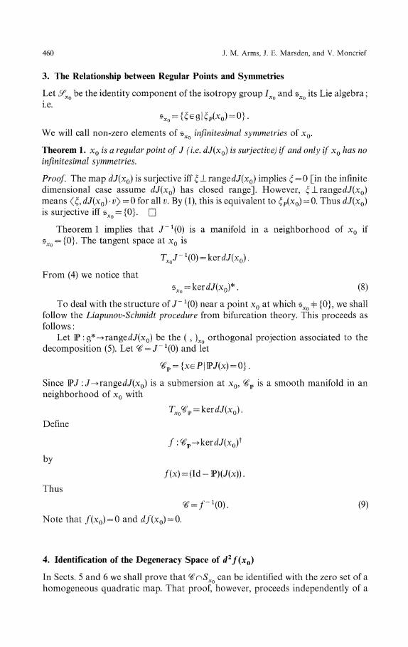
3. The Relationship between Regular Points and Symmetries
Let £fXQ be the identity component of the isotropy group IXQ and sxo its Lie algebrai.e.
We will call non-zero elements of sxo infinitesimal symmetries of x0.
Theorem 1. x0 is a regular point of J (i.e. dJ(x0) is surjective) if and only if x0 has noinfinitesimal symmetries.
Proof. The map dJ(x0) is surjective iff ξ JL range dJ(x0) implies ξ — 0 [in the infinitedimensional case assume dJ(x0) has closed range]. However, ξλ. range dJ(x0)means <ξ, dJ(x0) ι;> =0 for all v. By (1), this is equivalent to ξp(χ0) = 0. Thus dJ(x0)is surjective iff sxo = {0}. Π
Theorem 1 implies that J"1^) is a manifold in a neighborhood of x0 ifsxo = {0}. The tangent space at x0 is
From (4) we notice that)*. (8)
To deal with the structure of J~ 1(0) near a point x0 at which $xo Φ {0}, we shallfollow the Liapunov-Schmidt procedure from bifurcation theory. This proceeds asfollows :
Let IP :g*->rangedJ(x0) be the ( , )XQ orthogonal projection associated to thedecomposition (5). Let (β = J~1(Q) and let
Since PJ : J^ range dJ(x0) is a submersion at x0, is a smooth manifold in anneighborhood of x0 with
Define
by
Thus
Note that /(x0) = 0 and d/(x0) = 0.
4. Identification of the Degeneracy Space of d2f(xQ)
In Sects. 5 and 6 we shall prove that ^π5Xo can be identified with the zero set of ahomogeneous quadratic map. That proof, however, proceeds independently of a
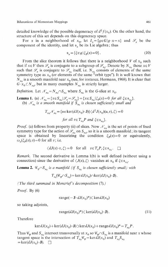
Bifurcations of Momentum Mappings 461
detailed knowledge of the possible degeneracy of d2f(x0). On the other hand, thestructure of this set depends on this degeneracy space.
For x in a neighborhood of x0, let Ix = {geG\g x = x} and 5 . be thecomponent of the identity, and let *x be its Lie algebra thus
*x = {ξeg\ξp(x) = 0}. (10)
From the slice theorem it follows that there is a neighborhood V of x0 suchthat if xe V then <?x is conjugate to a subgroup of £fXQ. Denote by NXQ those XE Vsuch that £fx is conjugate to £fXQ itself, i.e. NXQ consists of elements of the samesymmetry type as x0 (or elements of the same "orbit type"). It is well known thatNXQ is a smooth manifold near XQ (see, for instance, Hermann, 1968). It is clear thatG x0CNXQ, but in many examples NXQ is strictly larger.
Definition. Let Jf^ =JVV nSY where Sv is the G-slice at xn.J XQ XQ Xθ XQ V
Lemma 1. (a) ^eo = {χeSJCO|^e = 0} = {xεSJ(0|ξP(x)=0 for all ξesxo}.(b) JfKQ is a smooth manifold if Sxo is chosen sufficiently small and
Txo^x0 = {weker(dJ(x0)oJO| <d2J(x0)(u, t;), O =0
for all υeTXQP and £esxo}.
Proof, (a) follows from property (ii) of slices. Now JVXQ is the set of points of fixedsymmetry type for the action of ^XQ on SXQ, so it is a smooth manifold its tangentspace is obtained by linearizing the condition ξp(χ) = Q or equivalently,ωx(ξp(x),υ) = Q for all v; i.e.
υ,O=0 fora11 vεTxP,ξe*XQ. Π
Remark. The second derivative in Lemma l(b) is well defined (without using aconnection) since the derivative of <J(x), O vanishes at x0 if
Lemma 2. ^n^ is a manifold (if SXQ is chosen sufficiently small) with
(The third summand in Moncriefs decomposition (1).)
Proof. By (6)
range ( - JT° dJ(x0)*) C ker dJ(x0)
so taking adjoints,
range(^J(x0)*)Cker(^J(x0)oJJ). (11)
Therefore
ker dJ(x0) + ker(JJ(x0)o JJ) 3 ker JJ(x0) + range
Thus ^p and SXo intersect trans versally at x0 so nS^ is a manifold near x whosetangent space is the intersection of TXQ
(£]p = kerdJ(x()) and TXQSXQ
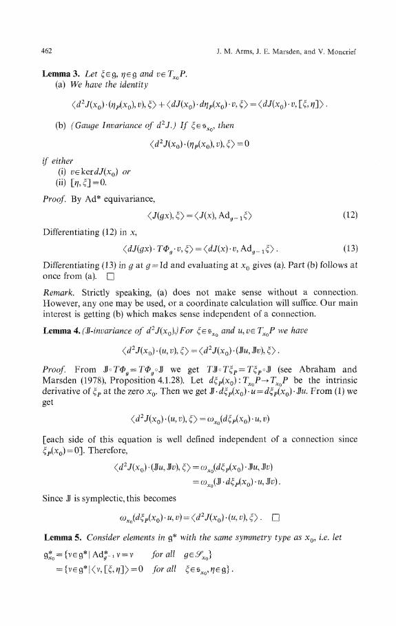
462 J. M. Arms, J. E. Marsden, and V. Moncrief
Lemma 3. Let ξe$, ηεg and veTXQP.(a) We have the identity
(d2J(x0) - (ηp(x0\ v\ ξy + <dJ(xσ) « dηp(x0) - ξ> = <dJ(xσ)' v> \ζ> Φ -
(b) (Gauge Invariance of d2J.) If ξesxo, then
if either(i) vekQΐdJ(xQ) or
(ϋ) fo,<3=0.
Proof. By Ad* equivariance
Differentiating (12) in x,
<^Jfex) - TΦ, -ϋ, O = <dJ(x) ϋ, Ad^_ XO . (13)
Differentiating (13) in g at g = Id and evaluating at x0 gives (a). Part (b) follows atonce from (a). Π
Remark. Strictly speaking, (a) does not make sense without a connection.However, any one may be used, or a coordinate calculation will suffice. Our maininterest is getting (b) which makes sense independent of a connection.
Lemma 4. (S-invariance of d2J(x0).)For ζ£*XQ and u,ve TXQP we have
(d2J(xQ) (u, v), ξy = <d2J(x0) - (Su9 Jfo), O.
Proof. From $*TΦg=TΦg*$ we get T$*TξP=Tξp°$ (see Abraham andMarsden (1978), Proposition 4.1.28). Let dξp(x0):TXQP-+TXQP be the intrinsicderivative o f ξ p at the zero x0. Then we get 3! dξp(x0) u = dξp(x0) lίu. From (1) weget
<d2 J(x0) (u, v\ ξy = ωxo(dξp(x0) - u, v)
[each side of this equation is well defined independent of a connection sinceζp(xo) = ϋ]. Therefore,
<d2 J(x0) - (Ju, Jί4 O - ωXo(dξP(xQ) Su, Sv)
= ωxo($ dξp(x0) u9$v).
Since Jί is symplectic, this becomes
ω*0(^P(x0) -^^) = <d V(x0) («, 4 O Π
Lemma 5. Consider elements in g* with the same symmetry type as x0, i.e. let
Ad*- ιV-v for all
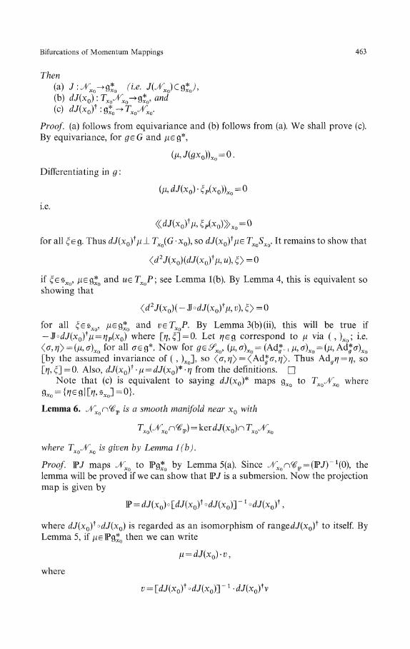
Bifurcations of Momentum Mappings 463
Then(a) J:^X0^Q*XO (ί.e. J(Λ"JCQ*J,(b)dJ(x0):TxoΛ χo-+Q*Xo,and(c) dJ(xoγ .9*xo-+TXoΛ χo.
Proof, (a) follows from equivariance and (b) follows from (a). We shall prove (c).By equivariance, for #eG and μeg*,
Differentiating in g :
.e.
for all ξe g. Thus dJ(x0)^μ _L TXQ(G x0), so d J(x0)^e TXQSXQ. It remains to show that
if ξesxo, μegJ0 and ueTXQPι see Lemma l(b). By Lemma 4, this is equivalent soshowing that
for all ξesxo, μeg*o and veTXQP. By Lemma 3(b) (ii), this will be true if— SodJ(xQYμ = ηP(xQ) where [)/,£] = 0. Let ^eg correspond to μ via ί,)^; i.e.<σ, ηy = (μ, σ)XQ for all σe g*. Now for ge ίfχo, (μ, σ)Xo = (Ad*- , μ, σ)Λo - (μ, Ad*σ)Xo
[by the assumed invariance of ( , )Xo], so <σ,?/> = <Ad*σ,77>. Thus Aάgη = η., so[//, ξ] = 0. Also, dJ(x^ - μ = dJ(xQ)* η from the definitions. Π
Note that (c) is equivalent to saying dJ(x0)* maps QXQ to TXQ^XQ where
Lemma 6. ^o^^p is α smooth manifold near XQ with
where TXQJfXQ is given by Lemma ί(b).
Proof. PJ maps jVXQ to Pg*o by Lemma 5(a). Since J^on<iflp = (PJ)~1(0), the
lemma will be proved if we can show that IP J is a submersion. Now the projectionmap is given by
P = dJ(x0) o [dJ(x0)t °dJ(*0)] '
ί °dJ(xoγ ,
where dJ(x0)to<l/(;x;0) is regarded as an isomorphism of range dJ(xQ)^ to itself. By
Lemma 5, if μePg*0 then we can write
where
464 J. M. Arms, J. E. Marsden, and V. Moncrief
for some vegjo. By Lemma 5 (b) and (c), veTXQ^VXQ. Thus μ = JPdJ(xQ)'V forVE TXQ^XO, so PJ is a submersion at x0. ΠXO
Lemma 7.
Proof. Notice that if ξe$xo and xeΛ^0 then dJ(x)*ξ = 0. Thus the x-derivative of<J(x), O vanishes identically on «yΓXo. Therefore, 0 = <J(x), £> for xeJVXQ andξeker^J(x0)*. Equivalently, 0 = ( J(x), v)XQ for xe^XQ and V6kerrfj(x0)
f. But thismeans that (/-P)(J(x)) = 0, so J(x) = 0 on Jf^rfβ^ Π
Thus, solutions of J(x) = 0 with the same symmetry type as x0 form a smoothmanifold. The proof of Lemma 7 also establishes the following :
Lemma 8. Consider the map f :^pnSXo-»ker<i7(;x0)t defined by
(as in Sect. 3). Then J^n^p is a manifold of critical points of f.
The degeneracy space of / at a critical point x is defined to be
{uεTx(VwπSXo)\d2f(x)(u,v) = Q for all veT^^SJ
Here is our second main result :
Theorem!. Λ^n^ is a manifold of non-degenerate critical points forf :^wnSXQ^kQΐdJ(x0)^ in the sense that
(a) each xeΛ^n^ satisfies df(x) = Qand
(b) the degeneracy space for f at xeΛ^n^7 equals Tx(JfXQr\^\
Proof. By Lemmas 7 and 8, (a) holds. Also, we have
<rf2/(*o) - (ii, v\ O = <d2J(x0) - (u, v), ξy (14)
for all ξe*x, and u9veTXQ(<#vnSXo). If weΓJΛ/^n^) then (14) vanishes byLemma l(b), so u lies in the degeneracy space for / at x0. Conversely, supposeue Txffi^r\SX() and u lies in the degeneracy space for / at x0 thus (14) vanishes forall ξesxo and all veTXo(<gvnSXQ). If w t e range (-J°dJ(x0)*) then<d2J(x0)(tί,w1), ξ>=0 by gauge invariance [Lemma 3(b)(i)]. Now the orthogonalcomplement of Txo(^?
lpn5:co)©range( — S°dJ(xQ)*) is range(rfj(%0)*) by Moncrief sdecomposition (7). For w2erange(ί?J(x0)*), <rf2J(x0)(w, w2), ξy = 0 byLemma 3(b)(i) and JJ-invariance. Thus <^2J(x0)(w,w), ξy=0 for all VETXQP, soweΓ^Λ^. Since all points of Λ^n^ have the same symmetry, the samecalculation works at any point xeΛ^n^. Π
The following special case is useful to note :
Corollary. // dimker(iJ(x0)* = 1, then Jf^c\^ is a nondegenerate critical manifoldfor f and so ^nSXQ is the product of a cone with (Λ^nS^) and hence Ή itself is acone x (^Xo(^SXQ) x (G/IXQ), in a neighborhood of x0.
The conclusion that ^nSXQ is a cone x J^XQr\SXQ follows from the parametrizedMorse lemma; cf. Bott (1954).
Bifurcations of Momentum Mappings 465
Example. Let H:IR2-»IR be a smooth hamiltonian with a critical point at theorigin. Suppose H has all its orbits periodic of the same period. Then H has a non-degenerate critical point at (0, 0). This follows from the corollary to Theorem 2 byusing G = S^ acting by the flow of XH. In fact, as we will see in Lemma 17 below,there are symplectic coordinates near (0, 0) in which H is homogeneous quadraticthus H is a harmonic oscillator.
5. Quadratic Momentum Mappings
Theorem 3 below proves that if / is quadratic then there is a diffeomorphism of aneighborhood of x0 that maps ^nSXo to the set of zeros of u\-*(I — lP)d2J(x0)(u,u)for ueTXQSXQ. Moreover, this diffeomorphism respects the information derived inTheorem 2 (see Theorems 4 and 4').
The case treated in this section applies to some interesting quadratic examples,such as gauge theories, as we shall see in Sect. 8. The proofs really only require that(Id — IP)/ restricted to SXQ is quadratic. This observation is applied to theconstraint equations in general relativity near a spacetime having k spacelikeKilling symmetries (the supermomentum constraint is quadratic, but theHamiltonian constraint is not).
The following elementary example shows that in general, zero sets of quadraticmaps need not have conical singularities thus, even when J is quadratic, it is notobvious that /"ΉO) has conical singularities.
Example. Let F:!R3-»IR2; F(x, y, z) = (x2 + y2 - z, x2 - yz) and consider F'^O)near (0,0,0). This set does not have a conical singularity, but rather a cuspsingularity z = y2 + y3 + . . ., x = y3/2 + . . . near (0, 0, 0).
The components of the momentum mapping are linked together in a nontrivialway by Ad*-equivariance. These extra properties actually rule out singularities ofhigher order than quadratic.
The key to the constructions in this section is the Kuranishi map used byAtiyah et al. (1978). We are grateful to L. Nirenberg and I. Singer for suggesting itsconsideration2. Kuranishi (1965) originally used this map (called F below) in astudy of deformations of complex structures.
Our assumptions are as in Sect. 2, except now let us assume that P is (open in) alinear space and J is quadratic; i.e., let J(x0) = Q and assume that in a neigh-borhood of x e P ,
where Q(h) = %B(h9h), and B(u,υ) = d2J(x0)(u,v).The map A = dJ(x0)°dJ(x0)'* is an isomorphism of rangerfJ(x0) to itself. Let
G = J ~ l o P: g* -> ranged J(x0), the "Green's function" for Δ. The crucial map wedeal with is
F-.P-+P
where h = x — x0.
2 Keep in mind the fact that the singularities found here do not occur in the Euclidean theorystudied by Atiyah et al. (1978)
466 J. M. Arms, J. E. Marsden, and V. Moncrief
Lemma 9. F is a local diffeomorphism of a neighborhood of x0 to a neighborhood of
*o
Proof. DF(x0) = Id. D
Lemma 10. F takes a neighborhood of x0 in Ήw to a neighborhood of x0 in{x0}+kerdJ(:x0).
Proof. We need to show that
xe^jpoF(x) — x0ekerdJ(x0) .
Now
But from the definition of G we have dJ(x0)°dJ(x0)toG = P and so
dJ(x0)(F(x) - x0) = dJ(x0) ft + Pβ(h)
. D
We now explicitly choose Sxo to be the affine slice; i.e. SXo is a ball in{x0}+ker(Λ7(x0)oJF).
Lemma 11. JF maps SXQ to SXQ.
Proof. For £eg and
= <d/(x0)oJΓ(Λ),O
because range (Jorf^XQj^ckerdJixo) implies that
<dJ(x0)oJoίi/(x0)toGoβ(Λχθ = 0. D
From Lemmas 10 and 11 we get
Lemma 12. F restricts to a local diffeomorphism of ^^r\SXQ to
{%0} +kerdJ(x0)nker(dJ(x0)oJί).
Note that this proof also shows that ^nS^ is a manifold; cf. Lemma 2.Lemmas 9-12 do not use the fact that J is quadratic; indeed, Q(h) can be
replaced by the remainder R(h) in the Taylor expansion. Now we shall use the factthat J is quadratic. [As we already remarked, it is noteworthy that we only need toassume that (Id — F)°J is quadratic.] Our main result of this section is as follows.
Theorem 3. The local diffeomorphism F maps ^nSXo locally 1 — 1 onto the cone
<d2J(x0)(w, u\ O=0 for all
Thus, locally Γ ^0) - # w CXQ x G//X0.
Bifurcations of Momentum Mappings 467
Proof. From Lemma 12, we need to show that for
(Id - F) Q(F(x) - x0) = 0^(Id - P)J(x) = 0. (16)
Keep in mind that (Id-P)J(x) = (Id-P)β(ft). By Lemma 10, F(x)-x0eker dJ(xQ)so letting P be the orthogonal projection onto ker dJ(x0), we have
F(x)-x0 = P(F(x)-x0)
= P(fc + dJ(x0)t°G°β(Λ))
= Wh.
Therefore,
(Id-P)β(F(x)-x0) = (Id-P)β(P/0
= (Id-P)β(Λ-(Id-P)Λ).
Since (Id — P)J is quadratic, this becomes
(Id-P)β(F(x)-x0)
= (Id- P){β(Λ)- B(h, (Id- P)Λ) + \ β((Id- P)h, (Id- P)Λ)} . (17)
By J-invariance of d2J(x0),
(Id - P)(£(Λ, (Id - P)Λ)) - (Id - P)(B(JTft, JJ(Id - P) A)) .
Now /ιeker(dJ(x0)°JJ) since xeS^, so Ji/ieker(dJ(x0)). Also,Jf(Id — P) foe range J°dJ(x0)*, so $(Id — W)h = ηP(xQ) for some ηe§. Therefore, bygauge invariance [Lemma 3(b) (i)],
A similar argument together with the fact that range ($°dJ(x0)*)C ker dJ(x0) showsthat
Thus from (17),(Id-P)β(F(x)-x0) = (Id-P)β(h),
which gives (16). QNext we show that F maps the degeneracy manifold to the affine space
determined by the degeneracy space of the second derivative.
Theorem 4. F maps Jf^r^ locally 1 — 1 onto the affine space
{x0} + {t/6ker(dJ(x0)oJJ)nker(^J(x0))| (d2J(x0)(u, υ\ ξ> -0
for all £ekerdJ(x0)* and all vεTXQP} = xon%XQ.
Proof. We already know that for xeSxn^, u=F(x)— x0eker(JJ(x0)°JJ)nker(dJ(x0))by Lemmas 10 and 11. Now suppose that xe«Λ^.0. Then by definition of F and Jϊ-invariance,
<d2J(xΰ)(u, v\ O = <d2J(x0)(h, v), ξ> + (d2J(x0)(dJ(xoγ °G°Q(h), v), O
468 J. M. Arms, J. E. Marsden, and V. Moncrief
Now JfXQ is an affine space, so he TXQ^VXQ. Thus by Lemma 5, G°Q(h)eQ*Q. Thus byLemma 3(b)(ii), the second term vanishes. The first term vanishes by Lemma l(b).Thus F maps J^n^ into the stated space. Since these spaces are tangent at x0
and F is a local diffeomorphism, the result follows. ΠTheorem 4 can be generalized as follows : let Jf C XQ be a Lie subgroup with
Lie algebra ί). Define £/.# = {xeP\dJ(x)*ξ = Q for all ξ e f y , an affine subspacethrough x0, let &^ = £/^πSXQ and let CXQ be the cone in Theorem 3.
Theorem 4'. We have F(jtf#) = jtf#, F(^^) = &*> and so F(g&#n<#) = 3S#nCXQ in aneighborhood of x0.
Thus, F preserves symmetry type for any subgroup of έfXQ. Theorem 4 is thecase 3? = SfXQ. [Note that as above, we need only assume (Id — F)J|SΛo isquadratic.]
Proof of Theorem 4'. Since s/# is affine, xestf^ if and only if (d2J(x0)(h,v\ O =0for all veTXQP and £eϊ), where h = x — x0. Then if u = F(x) — x0,
<d2 J(x0)(u, ι>), O = <d2 J(x0)(h, ϋ), O + <d2 J(x0)(^J(x0)t o Goβ(h), ι>), O .
The first term vanishes by assumption. Since ί) C sxo, the argument in the proof ofTheorem 4 shows that the second term vanishes as well. Thus JF( j^) C si#. SinceDF(x0) = Id, we have local equality. The remaining assertions follow fromLemma 11 and Theorem 3. Π
6. General Momentum Mappings
We shall now obtain the conical structure of J~ 1(Q) without the assumption that Jis quadratic. The methods of this section do not rely on those in the previous one.However, the methods here have the disadvantage that they are more difficult toimplement in the infinite dimensional case. The examples given in Sect. 8 use theresults of the previous section rather than this one. In particular, the method usedhere relies on the Darboux theorem a version of this theorem that is useful ininfinite dimensional problems is technically quite complicated (see Marsden, 1980,Sect. 1).
The strategy in this section is to show that j = (ld—!P)J\((£vΓ(SXQ) is themomentum map for the action of ^XQ. This action has a fixed point at x0 and theDarboux Theorem can be used to find symplectic coordinates in which the actionis linear and hence in which j is quadratic.
Lemma 13. ^pr\SXQ is a symplectic submanifold of P.
Proof. In Lemma 2 we showed that ^^SXQ is a manifold. It suffices to show thatthe symplectic form restricted to T,Co(
(^7
pnSί
JCo) is non-degenerate. LetuekerdJ(x0)nker(dJ(x0)°J) and suppose that
for all v in the same space. But «w,Jίw1»=0 for w x eRange$°dJ(x 0 )* and<<χjΓw2»=0 for w2e RangedJ(x0)*. Thus, by Moncriefs decomposition (7),«M, Jfo» = 0 for all ve TXQW and so u = 0. Π
The preceeding lemma is implicit in Marsden-Weinstein (1974).
Bifurcations of Momentum Mappings 469
Lemma 14. Let RcP be a symplectίc submanίfold and H C G a subgroup leaving Rinvariant. Then the momentum map of the H action on R is j = πl)°J°iR whereiR : R^P is inclusion, and π^ : cj*— »ί)* is the natural projection. If the momentum mapJ of the action is Ad*-equivariant, then so is j.
This is a straightforward verification from the definition of momentummappings (1).
Lemma 15. &XQ leaves ^wr^SXQ invariant and has a fixed point at XQ.
Proof. First of all, £fXQ leaves SXQ invariant by property (i) of the slice (see Sect. 2).Next, suppose that xe<#vι i.e. PJ(x) = 0. Then for g e ί f χ o , WJ(gx) = W Ad*-ι J(x).Thus the proof is complete if we can show that P Ad*- 1 = Ad*- 1 IP. But thisfollows from the facts that P is an ( , )XQ orthogonal projection and that ( , )XQ isAd*- 1 -in variant for gε^XQ (see assumption 5 in Sect. 2). Π
Combining Lemmas 13-15, we obtain the following:
Lemma 16. The momentum mapping for the action of ^Xo on ^PnSXo is
Lemma 17. There is a symplectic change of coordinates on ^wnSXQ (the coordinatechange has derivative the identity at x0) in which the action of &XQ is linear, andhence j is homogeneous quadratic, since j(xQ) = 0 and dj(xQ) = 0.
Proof (see Weinstein, 1977, p. 24, last paragraph). Let Ω0 be the symplecticform on ^pnSXo (Lemma 13) and let Ω1 be the (constant) symplectic form onTXo(%>wπSXo). Let exp : TXQ(^^SX^^^SXQ be the exponential map associated tothe metric « , ». Since the action Φg preserves « , » then for ge^XQ,
Φg°exp = exp°TΦg(x0). (18)
By the proof of Darboux' theorem (Weinstein, 1977, pp. 22-23) there is a localdiffeomorphism f1 of ^wnSXQ to itself such that
^Ωo (19)
and fsΦβ = Φg°fι. Let /2 = exp - 1 ofί then by (18)
f2°Φβ°fϊ1 = TΦβ(xo). (20)
Also, by (19), /2 gives a symplectic chart. Thus (20) shows that Φg is a linear actionin the new coordinates. Since the new coordinates are symplectic, (1) shows thatj isquadratic. Q
Thus, we have proved the following :
Theorem 5. There is a local diffeomorphism F of ^^r\SXQ that takes ^nSXQ locally1 — 1 onto the cone
<d2J(x0)(w,z4O=0 forall
ThusVκCXQx(G/IXQ).
470 J. M. Arms, J. E. Marsden, and V. Moncrief
7. Discussion
This section discusses several ways of interpreting and using the results obtained.
a) Bifurcations
Following Smale (1970), we define a bifurcation point of a map / : M-+N to be apoint y0e.N such that f~l(y) changes topological type as y varies in someneighborhood of y0 [see Marsden (1978) for a discussion of this definition]. Ifsome uniformity condition on the derivative of / is made (e.g. if M is compact)then no regular point can be a bifurcation point (by the implicit function theorem).Theorem 1 shows that for momentum maps, the only candidate bifurcation pointsare images of points with symmetry group of dimension ^ 1.
In topology and mechanics one is interested in how the level sets of themomentum map fit together. The reason is simply that any Hamiltonian systemleaves these sets invariant, so a knowledge of the topology of those sets can yieldinformation about the flow. Complications in the topology occur precisely atbifurcation points, by definition. In determining this complication, the structure ofJ~1(μ0) at the bifurcation point μ0 is the crucial information needed. Ourtheorems determine precisely the local structure of J~ 1(0) when 0 is a bifurcationpoint.
b) Linearization Stability
Let F:M->N be a smooth map and let x0eM and yQeF(x0}. LetTXQF : TXΌM-*TyoN denote the tangent (derivative) of F. A vector /zekerTXoF iscalled integrable if it is tangent to a C1 curve x(λ) in F~1(yQ). We call Flinearization stable at x0 if every /ιekerTXoF is integrable. This notion arose fromperturbation theory in general relativity and was first introduced in Fisher andMarsden (1973). The work was motivated by Brill and Deser (1973). Theconnection with symmetries was made by Moncrief (1975a). If one seeks solutionsx of F(x) = y0 near to x0, and if F is linearization stable at x0, these solutions can beobtained in the form x = x0 + λh -f 0(λ2) for any hekQΐTXQF.
If 3/Q is a regular value of F, then F is linearization stable at XQ by the implicitfunction theorem. Suppose, however, that y0 is not a regular value of F. Then if/ιekerTXQF is integrable, it satisfies the necessary second order condition
for any /e TyoN that annihilates the range of TXQF. (The second derivative on / iswell defined since (I, TXQF hy=0.) This is obtained by differentiating F(x(λ)) = yQ
twice.Theorems 3 and 5 imply that if F = J is an Ad*-equivariant momentum
mapping (associated with a group admitting a slice), and J(χ0) = 0, then the abovesecond order condition is not only necessary for integrability, of /zekerrfJ(x0), butis sufficient as well. This is basically another way of saying that the singularities inthe set J"1^) are homogeneous quadratic.
Bifurcations of Momentum Mappings 471
c) Reduction
Singularities can occur when one reduces a Hamiltonian system with symmetries.Suppose that (P, ώ) is a symplectic manifold and that G acts on P and has an Ad*-equi variant momentum map J :P— >g*. The first step in reduction (see Marsdenand Weinstein, 1974) is to study the level surfaces of J. The proof of Theorem 1shows that if J(xQ) = μ0, then x0 is a regular point of J if and only if x0 has noinfinitesimal symmetries. In the regular case, J~ I ( x 0 ) is a manifold near x0 and onecan then proceed with reduction to get the symplectic manifold Pμo = J~~1(μQ)/Gμo.If, however, sXo = keri/J(x0)*=t={0} then singularities in J~1(μ0) will occur at x0
(unless the cone CXQ described in Theorem 3 happens to be a single point), and sothe usual method of reduction does not apply. However, the set <Λ^Xon%? = J^xor\(&w
= N XQΓ\S XQΓ\^ is a manifold near x0 (see Lemmas 6 and 7) with tangent space
where TXQ^V is given by Lemma l(b). In fact, it is a symplectic submanifold of P.
Lemma 18. Assume J(x0) = 0. Then JfXQr\^ is a symplectic submanifold of P.
Proof. It suffices to show that the symplectic forms restricted to Txo(yi^on^) isnondegenerate. Let ueTXQ(JΓXQr\^)
(x0)(w,ι;), ξ> -0 for all t e TXQP and ξesxo}. Wewant to show that ωxo(w,ϊ;) = <^tt,Jίί;>>=0 for all ι;GTXo(Λ^on#) implies that w = 0.To see this note that if we Tx (Λ^n^) then Su lies in the same space. This followsfrom the Jί-in variance of d J(x0) (see Lemma 4). Thus, putting v = JJw, we get0 = ωxo(u, Su) = «M, JJ2w» - - «χ M>>. Thus u = 0. Π
If H : P->R is a G-invariant Hamiltonian then the flow Ft of the correspondingHamiltonian vector field XH commutes with the action, so it leaves eachsubmanifold Nxo of points with the same symmetry type as x0 invariant. It alsoleaves Nγ n^ invariant, since J is conserved. The dynamics on N n^can be
XQ J XQ
reconstructed from the dynamics on (NXon<<ί)/G««yΓ;Con# as in Abraham andMarsden (1978, pp. 304-305). But the flow on Λ^on# isjust the Hamiltonian flowof the Hamiltonian ff|(^on^). Thus, while bifurcations can occur in the fullspace #, reduction can still be done to obtain a Hamiltonian system on points withthe same symmetry type as x0. This procedure is useful, for example, when passingfrom the general Einstein equations to obtain a Hamiltonian structure forhomogeneous cosmologies (cf. Jantzen, 1979).
d) Constraints in Field Theories
The reduction procedure or the topological program in mechanics naturally leadsone to study the level sets J~l(μ) of a momentum mapping. Here it plays the roleof a conserved quantity in a mechanical system. However, in relativistic fieldtheories, the zero set of a momentum map can often be identified with theconstraint set in the sense of the Dirac theory of constraints. For relativity, therelevant group is the group of diffeomorphisms of spacetime and for gaugetheories it is the group of bundle automorphisms (covering the identity if thetheory is not coupled to gravity). In fact, in Gotay et al. (1980) it is shown that this
472 J. M. Arms, J. E. Marsden, and V. Moncrief
is the case for a wide variety of field theories (essentially any theory which is firstclass in the sense of Dirac)3. Thus, the results of this paper can be used to analyzethe singularities that occur in spaces of solutions of relativistic field theories. Howto do this for gauge theory and relativity will be outlined in the next section. It maybe useful to attempt to resolve the singularities in the constraint sets by realizingthem as projections of smooth Lagrangian submanifolds. It is not clear how to dothis in detail, but the work of Kijowski and Tulczyjew (1979) may provide thecorrect context.
8. Examples
This section gives three applications of the general theory. Very likely there areseveral more of considerable interest. For example, bifurcations of the zero set oftotal angular momentum seem to play a role in the studies of Brown and Scriven(1980).
a) Angular Momentum of N particles
Let P= T*IR3]V^1R6]V be the phase space for N non-relativistic particles (allowingseveral particles to occupy the same position in R3). Consider the usual action ofSO (3) on P. The associated momentum map is the total angular momentum J ofthe system. In terms of standard coordinates (xja), P(α)), α=l, . . . ,ΛΓ, we have
Γ— V PlJkγJ Dk
J — L b X(a)P(a)a,j,k
or
The level surfaces of the momentum map
will have singularities exactly at the points admitting nontrivial isotropy groups.The only point invariant under the full SO(3) action is clearly x(α) = 0, p(Λ)=0.Other points having nontrivial isotropy groups have the form x(α) = αfln, p(fl) = βan,where n is a unit vector in R3 and αfl and βa are constants (not all zero). Each suchpoint is invariant under the circle action of rotations about the axis h. The"degeneracy manifold" of points admitting such 1 -dimensional isotropy groups is2N + 2 dimensional. Note that each such point has J = 0. We can expect that acone of solutions of the equation J = Q branches from each such symmetric point(for the case N> 1) since one can clearly have two or more particles each with non-vanishing individual angular momentum, but J = 0 by cancellation.
3 Relativistic fluids are covered if a suitable Hamiltonian formalism is used. Even in the "standard"formalism (see Hawking and Ellis, 1973), there are still singularities in the reduction process eventhough the equations themselves are linearization stable. The failing of the "standard" formalism is thatit does not write the constraints as the zero set of a momentum mapping. This can be done with theright choice of variables; cf. Arms (1979b)
Bifurcations of Momentum Mappings 473
The case N = 1 is special, but also is interesting. Here
is a cone over a smooth compact 3-manifold M. In fact, it is not hard to see thatM is (S2 x Sl}/~ where ~ identifies simultaneous antipodal points in S2 x S1.
[There is no bifurcation from non-zero points (x9p)eJ~1(0) since all suchpoints have the same symmetry here NXQ coincides locally with J~ 1(Q). For N > 1this accident does not occur.]
b) Gauge Theory
Existence and uniqueness theory for the Cauchy problem shows that the structureof singularities in the solution space of the four dimensional Yang-Mills fieldequations on a fixed background spacetime is the same as that for the constraintequations. These constraint equations are well-known and may be described asfollows (see, for example, Arms, 1979a): Let M be a fixed compact 3-manifold (aCauchy surface in the fixed background spacetime). Let π : B-+M be a principle G-bundle and let 2ί denote the space of (Ws'p, s > 3/p + 1) connections on this bundle.Elements ,4e2I represent vector potentials for gauge fields restricted to M. LetP=T*$I be the basic symplectic space, elements of which are pairs (A,η); ηrepresents the generalized electric field density. Assume g, the Lie algebra of Gcarries an adjoint-action invariant inner product ( , ), so TU>I/)(T*9I) [elements ofwhich are denoted (b,θ)] carries a preferred L2 inner product « , ». This, thecanonical symplectic structure and the complex structure JJ(b, θ) = ( — θ, b)[appropriately dualized by ( , )] are in the correct relationship (2).
The constraint equations are J(A,η) = 0 where J(A,η) = dη + [AΛη~] is thegauge covariant divergence of η using the connection A. In fact, J is themomentum map for the action of the group ^ of bundle automorphisms of B on P.This is the group G in the general theory; its Lie algebra is g, the g-valuedfunctions on M. The dual g* is the g* valued densities thus J : P-+g*. The adjointoperators dJ(A, η)* and dJ(A, η)+ are elliptic and so one can construct a slice usingkeΐ(dJ(A,η)°$). In fact, all of the assumptions of Sect. 2 hold; the spaces here areinfinite dimensional but ellipticity of dJ(A, η)* validates the technical points.
Moreover, J is quadratic. The quadratic term g of Sect. 5 is
where b and θ are perturbations of A and η,soh = (b, θ\ and [b Λ θ~\ is the bracket ing. (From this simple form gauge and JJ-invariance can be verified directly.)Theorem 3 therefore directly applies. For gauge fields, infinitesimal symmetries of(A, η) are ,4-co variant constant g-valued functions on B that commute with η. Theexistence of such symmetries implies that the gauge field is reducible to a field witha smaller gauge group HcG, HΦG. The space Λ^^π^7 of Sect. 4 consists ofsolutions of the constraint equations which are reducible to the gauge group Hthe rest of the solution set containing the conical singularities consists of solutionswith a gauge group K intermediate between H and G, Theorem 4' then shows howconical singularities of specified symmetry type K fit together to produce the entire
474 J. M. Arms, J. E. Marsden, and V. Moncrief
conical singularity in the constraint set ($ = {(A, η)\J(A9 η) = Q}. For more details,see Arms (1980).
For noncompact M, symmetries often are associated with a gauge groupgenerating a momentum map representing a total energy-momentum tensor orcharge. Such symmetries need not lie in the group generating the constraints, soneed not indicate singularities in the space of solutions. (For example, in generalrelativity, Minkowski space is a regular point in the space of solutions of Einstein'sequations.) For Yang-Mills fields however it is interesting to impose the constraintthat the color charge q vanish for non-compact M, say M = R3. This is suggestedby the classical limit of a quantized Yang-Mills theory with the property of"confinement".
Consider then a classical Yang-Mills theory on M = 1R3 with the constraintg = 0 added on, where
=- j \_A/\η\.M M
[This procedure is to be done in the appropriate weighted Sobolev spaces toproperly capture the asymptotic behavior; cf. Cantor (1979).] There is now asingularity in the space of all solutions at the trivial "vacuum" solution A = Q,η — 0 the constraint q = 0 leads to the second order condition
M
to be placed on first order perturbations, as in the compact case. Thus it seems thatan appropriate free field approximation to the nonlinear theory is not the usuallinearized Yang-Mills equations, but rather these equations supplemented by theabove second order condition.
c) The Constraint Equations in General Relativity
We shall use the methods of Theorem 3 to study the conical singularities in theconstraint equations of general relativity. Let M be a compact 3-manifold and Jt
the space of Ws'p,s> - +1 Riemannian metrics on M and let P=T*Jί denote\ P I
the "natural" cotangent bundle of Jί i.e. the fiber of Ύ*Ji over geJt consists ofall symmetric 2-contravariant tensor densities π (of class Ws~1>p). The constraintset of the vacuum Einstein equations on a 4 dimensional spacetime in which M isembedded as a compact hypersurface is well known to be the set
where Φ : T*Jl-+ (Densities on M) x (One-form Densities on M) is defined by)) and tf and / are given by
, π) = {(π' π' - £ (trace π')2) - R(g)} μ(g)
and
Bifurcations of Momentum Mappings 475
Here π = π' ®μ(g\ μ(g) is the volume form of g, and R(g) is the scalar curvature of g.In Fischer et al. (1979) it is shown that # has a conical singularity at (g0,π0) if
(00, π0) is the Cauchy data for a spacetime with one Killing field (either timelike orspacelike). Here we show the same thing if there are k spacelίke Killing fields. Weshall assume that trace π' = constant on M (i.e. M is a hypersurface of constantmean curvature in the spacetime). Then, the aforementioned reference establishesthe analogue of Eq. (8), namely that ker(DΦ(00, π0)*) is /c-dimensional and isspanned by elements of the form (0,Xα), a = 1, . . . , k where Xa is a vector field on Msatisfying LXaπ0 = 0 and LXag0 = 0. The adjoint is taken relative to the L2 metric onT*Jί given by
«(Λ1,ω1),(Λ2,ω2)»= J {h^h2 + ω^ω2}μ(g),M
where " " denotes contraction using g [(#, π) is the base point] and the naturalpairing between (Densities) x (One-form Densities) and (Functions) x (VectorFields). Thus DΦ(g,π)*: (Functions x Vector Fields) ->T(^π)(Γ*^), and one cancompute this explicitly.
At this point we are not claiming that Φ is a momentum map for a groupaction. If we were dealing only with the momentum contraint /, the results ofTheorem 3 would apply directly since the momentum map for the action of thediffeomorphism group of M on T*Jt is just the quadratic map J : T*^-» (vectorfields)*; (J(g,π),Xy= J X - /(g, π) = 2 J (Lxg) - π. However the Hamiltonian con-
M M
straint ffl = 0 complicates this program.Decomposition (7) is known to hold for Φ (see Moncrief, 1975b Arms et al.,
1975; Fischer et al., 1979)
T(g >π)(T*M) = range( - $DΦ(g, π)*)0 range DΦ(g9 π)*
)] (21)
since range $DΦ(g0, π0)* CkerDΦ(#0, π0) and DΦ(g0, π0)* is elliptic. Here S(g>n)(h, ω)= (ωb, — /zfl), ίlfand b denote the raising and lowering of indices using the metric g.
Let
s(go,«o) = {(#o> πo)l + a neighborhood of zero in kerDΦ(#0, π0)° $ .
This makes sense since M is open in S2(M), the covariant symmetric two tensorson M, and so Ί*Jt is open in the linear space S2(M) x S^(M), where S%(M) is thespace of contravariant symmetric two tensor densities (S(go πo) plays the role of aslice for the four-dimensional diffeomorphism group of spacetime). The analogueof JVXQ (see Lemma 1) is
flf = LXβπ = 0 , f l = l , . . . , k and fo
Fischer et al. (1979) shows that ^(go^o} is a smooth manifold.Now define the local diffeomorphism F of T*Jί to T*Jί near (00,π0) as
follows. First, let,
476 J. M. Arms, J. E. Marsden, and V. Moncrief
Since DΦ(gQ, π0)* is an elliptic operator, A is an isomorphism of range DΦ(g0, π0)to itself. Following what we did in Sect. 5, let P denote the orthogonal projectionto range DΦ(#0,π0) and set G^Δ~l°W. Write h = (g, π) — (g0, π0) and let theremainder be given by
Next define F by the analogue of (15):
F(g, π) - (0, π) + DΦ(g0, π0)* o G o jR(Λ) .
Computations based on the results of Fischer et al. (1979) together with argumentslike those in Sect. 5 establish the following :
1. DF(g0, π0) — identity, so F is a local diffeomorphism.2. F maps S(go>πo) to itself.3. If = {(#, π) 1 PΦ(#, π) = 0}, which is a smooth manifold in a neighborhood
of (00, π0), then F maps in a 1 — 1 way onto a neighborhood of (00, π0) in (00, π0)+ kerDΦ(#0,π0).
4. F maps ^PnS(00>πo) to {fe0,Now define the cone
This is a cone because of the following crucial fact :
(Id-P)JR = (Id-P)Φ is quadratic in (g,π).
This is because (Id — P) projects to the span of {(Q,Xa)\a= 1, . . ., k} and so only thesupermomentum component / is involved in (Id — P)Φ. Thus one can effect thelast step in Sect. 5 :
5. F maps *nS(gθfπo) locally 1-1 onto C(ί?o>πo).The proof of Theorem 3 needs not only (Id — P)Φ to be quadratic but also
crucially uses JΓ invariance and gauge invariance of (Id — P)D2Φ(#0,π0). The J-in variance results from a direct computation using the expression for ^X-/(g,n)given above. The gauge invariance also can be proven directly see Fischer et al.(1979) for the general proof of gauge invariance of D2Φ. This reference alsoexplains how to remove the gauge condition S o πo).
Theorems 4 and 4' also carry over for this example. One of the crucial facts inthis regard is Lemma 5, which can be interpreted as a covariance property. Inparticular, it entails that φ*F(g, π) = F(φ*g, φ*π) for a diffeomorphism φ such thatφ*g0 = g0, φ*π0 = π0. For this example these may be proved by a directcalculation.
These results describe, for example, the structure of the space solutions nearBianchi IX models, such as the Taub universe (k = 4), the Kasner solution (fe = 3) orthe Gowdy solutions (fc = 2), cf. Jantzen (1979). In Arms et al. (1980) we shallgeneralize these arguments to allow a time-like Killing field as well as severalspacelike Killing fields. The flat space time T3 x IR is an especially interestingbifurcation point.
Bifurcations of Momentum Mappings 477
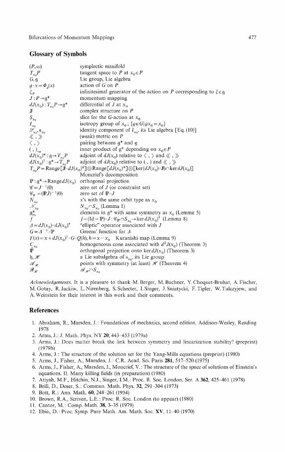
Glossary of Symbols
(JP, ω) symplectic manifoldTXQP tangent space to P at xQePG, Q Lie group, Lie algebrag x = Φg(x] action of G on Pξp infinitesimal generator of the action on P corresponding to ξe§J : P— >g* momentum mappingdJ(x0) : TXQP-+Q* differential of J at XΌ
$ complex structure on PSxo slice for the G-action at XQ
Ixo isotr opy group of x0 {g e G | gx0 = x0 }^0,5XQ identity component of IXQt its Lie algebra [Eq. (10)]
(weak) metric on Ppairing between g* and ginner product of g* depending on xQ<=P
dJ(x0)* : g-+TXQP adjoint of dj(x0) relative to < , > and « , »dJ(xoy : g*^TλoP adjoint of dj(x0) relative to ( , ) and « , »TXoP - Range [Jί»dJ(x0)*'] ® Range μj(*0)*] ® [ker (dJ(x0) ° JJ)nker dJ(x0J]
Moncrief s decompositionIP : g*-» Range dJ(xϋ) orthogonal projection(& = J~1(Q) zero set of J (or constraint set)<&r = OP./Γ HO) zero set of IP° JNxo x's with the same orbit type as x0
Λς°0 NX0^SXO (Lemma 1)gjo elements in g* with same symmetry as x0 (Lemma 5)/ /=(Id-IP)°J:%pnSXo->kerdJ(x0)
t (Lemma 8)Δ = dJ(x0)°dJ(xQ)* "elliptic" operator associated with JG = A ~ l off Greens' function for ΔF(χ) = χ + dJ(xoγ o G o Q(h), h = x-x0 Kuranishi map (Lemma 9)Cxo homogeneous cone associated with d2J(x0) (Theorem 3)IP orthogonal projection onto ker<ij(x0) (Theorem 3)ί), 3tf a Lie subalgebra of SXQ, its Lie groups$ ' # points with symmetry (at least) Jf7 (Theorem 4)
Acknowledgements. It is a pleasure to thank M. Berger, M. Buchner, Y. Choquet-Bruhat, A. Fischer,M. Gotay, R.Jackiw, L.Nirenberg, S. Schecter, I. Singer, J. Sniatycki, F. Tipler, W. Tulczyjew, andA. Weinstein for their interest in this work and their comments.
References
1. Abraham, R., Marsden, J. : Foundations of mechanics, second edition. Addison-Wesley, Reading1978
2. Arms, J.: J. Math. Phys. NY 20, 443-453 (1979a)3. Arms, J.: Does matter break the link between symmetry and linearization stability? (preprint)
(1979b)4. Arms, J. : The structure of the solution set for the Yang-Mills equations (preprint) (1980)5. Arms, J., Fisher, A., Marsden, J.: C.R. Acad. Sci. Paris 281, 517-520 (1975)6. Arms, J., Fisher, A., Marsden, J., Moncrief, V. : The structure of the space of solutions of Einstein's
equations. II. Many killing fields (in preparation) (1980)7. Atiyah, M.F., Hitchin, N.J., Singer, I.M.: Proc. R. Soc. London, Ser. A 362, 425-461 (1978)8. Brill, D., Deser, S. : Commun. Math. Phys. 32, 291-304 (1973)9. Bott, R.: Ann. Math. 60, 248-261 (1954)
10. Brown, R.A., Scriven, L.E. : Proc. R. Soc. London (to appear) (1980)11. Cantor, M.: Comp. Math. 38, 3-35 (1979)12. Ebin, D.: Proc. Symp. Pure Math. Am. Math. Soc. XV, 11-40 (1970)
478 J. M. Arms, J. E. Marsden, and V. Moncrief
13. Fischer, A., Marsden, J.: Bull. Am. Math. Soc. 79, 995-1001 (1973)14. Fischer, A., Marsden, J., Moncrief, V.: Ann. Inst. Henri Poincare (to appear) (1980)15. Gotay, M., Marsden, J., Sniatycki, J.: Lagrangian field theory and zero sets of momentum maps (in
preparation) (1980)16. Gotay, M., Nester, J., Hinds, G.: J. Math. Phys. NY 19, 2388-2399 (1978)17. Hawking, S., Ellis, G.: The large scale structure of spacetime. Cambridge: Cambridge University
Press 197318. Hermann, R.: Differential geometry and the calculus of variations, New York: Academic Press
1968, second edition by Math. Sci. Press 197719. Jantzen, R.: Commun. Math. Phys. 64, 211-232 (1979)20. Kijowski, J., Tulczyjew, W.: A symplectic framework for field theories. Springer Lecture Notes in
Physics, No. 107. Berlin, Heidelberg, New York: Springer 197921. Kuranishί, M.: New proof for the existence of locally complete families of complex structures. Proc.
Conf. on Complex Analysis. A. Aeppli et al. (eds.). Berlin, Heidelberg, New York: Springer 196522. Marsden, J.: Bull. Am. Math. Soc. 84, 1125-1148 (1978)23. Marsden, J.: Geometric methods in mathematical physics. CBMS Conf. Series (to appear) (1980)24. Marsden, J., Weinstein, A.: Rep. Math. Phys. 5, 121-130 (1974)25. Moncrief, V.: J. Math. Phys. NY 16, 493-498; 17, 1893-1902 (1975a)26. Moncrief, V.: J. Math. Phys. NY 16, 1556-1560 (1975b)27. Moncrief, V.: Ann. Phys. 108, 387-400 (1977)28. Moncrief, V.: Phys. Rev. D 18, 983-989 (1978)29. Palais, R.: Mem. Am. Math. Soc. No. 22 (1957)30. Segal, I.E.: Proc. Nat. Acad. Sci. USA 15, 4638-4639 (1978)31. Smale, S.: Inventiones Math. 10, 305-331; 11, 45-64 (1970)32. Souriau, J.M.: Structure des systemes dynamique. Paris: Dunod 197033. Weinstein, A.: Lectures on symplectic manifolds. CBMS Conf. Series No. 29, AMS (1977)
Communicated by A. Jaffe
Received January 31, 1980
Note added in proof. A very interesting example of a conical singularity in the angular momentumlevel surfaces of the spherical pendulum and its relation to action-angle variables is contained in thepreprint of H. Duistermaat, "On global action angle coordinates".
2. Results on the symplectic structure on the solution space of the Yang-Mills equations at regularpoints, which reproduce the theorems of Ref. [24, 27] (but from the spacetime rather than dynamicalpoint of views) are contained in Ref. [30] and in:34. Garcia, P., Rendon, A.P.: Reducibility of the symplectic structure of minimal interactions. In:
Lecture Notes in Mathematics, Vol. 676. Berlin, Heidelberg, New York: Springer 197835. Garcia, P.: Tangent structure of Yang-Mills equations and Hodge theory. In: Lecture Notes in
Mathematics, Vol. 836. Berlin, Heidelberg, New York: Springer 1979