tanagra perfs comp svm -...

Tanagra R.R.

5 juillet 2009 sur 16

1 Subject

Comparison of SVM implementations (Support Vector Machine) on large dataset.

Support vector machines (SVM) are a set of related supervised learning methods used for

classification and regression. Viewing input data as two sets of vectors in an n‐dimensional space, an

SVM will construct a separating hyperplane in that space, one which maximizes the margin between

the two data sets. The original optimal hyperplane algorithm proposed by Vladimir Vapnik in 1963

was a linear classifier. However, in 1992, Bernhard Boser, Isabelle Guyon and Vapnik suggested a

way to create non‐linear classifiers by applying the kernel trick (originally proposed by Aizerman et

al.) to maximum‐margin hyperplanes. The resulting algorithm is formally similar, except that every

dot product is replaced by a non‐linear kernel function. This allows the algorithm to fit the

maximum‐margin hyperplane in the transformed feature space. The transformation may be non‐

linear and the transformed space high dimensional; thus though the classifier is a hyperplane in the

high‐dimensional feature space it may be non‐linear in the original input space

(http://en.wikipedia.org/wiki/Support_vector_machine).

Our aim is to compare various free implementation of SVM, in terms of accuracy and computation

time. Indeed, because the heuristic nature of the algorithm, we can obtain different results

according to the used tools on the same dataset. In fact, in the publications describing the

performance of SVM, we should not only specify the parameters of the algorithm but also indicate

what is the tool used. This latter can influence the results.

SVM is very effective in domains with very high number of predictive variables, when the ratio

between the number of variables and the number of observations is unfavorable. In the other hand,

when the number of instances is high compared to the number of descriptors, it is not really

attractive in comparison to well known approaches such as logistic regression or linear discriminant

analysis. We are in a domain which is particularly favorable to SVM in this tutorial. We want to

discriminate two families of proteins from their description with amino acids. We use sequence of 4

characters (4‐grams) as descriptors. Thus, we can have a large number of descriptors (31,809) in

comparison to the number of examples (135 instances).

From a certain point of view, we deal with a large dataset here. But unlike the standard situation we

have a high number of variables. It is interesting to study the behavior of the tools in this situation.

Most of the tools load the whole dataset into the main memory. The memory ability of the

computer is then the main bottleneck. The feasibility of the computation relies of the utilization of

the memory, in addition to the dataset, during the learning process.

We use the OS information for measuring the memory occupation. About the calculations time, we

use the information supplied by the tools or, if it is not available, we use a chronograph. This is not

very accurate, but this is the order of magnitude that is most important.

Tanagra R.R.


We use a 5 fold cross validation for the error rate estimation. We cannot control the subdivision

according the tools. But, the results remain comparable. These are the large deviations that are

interesting to analyze.

We use the following tools:

Software Version URL

ORANGE 1.0b2 http://www.ailab.si/orange/

RAPIDMINER Community Edition 4.2 http://rapid‐i.com/

TANAGRA 1.4.27 http://eric.univ‐lyon2.fr/~ricco/tanagra/

WEKA 3.5.6 http://www.cs.waikato.ac.nz/ml/weka/

Other tools have been tested. They failed during the data loading or during the learning process. We

will list them below. It is possible that these failures are due to misuse or improper. This cannot be

excluded. The data file of this tutorial is available online. Anyone can carry out the same experiment

and probably find the right settings.

This document fills out the tutorials dedicated to the comparison of tools1.

2 Dataset

We deal with a protein classification problem. We want to discriminate two families of proteins from

their description, a sequence of 4 amino acids. Because, there are 20 kinds of amino acids, the

theoretical number of descriptors is 204 = 160.000. Many of them are not present in the dataset. We

have "only" 31809 descriptors. There are 135 instances.

The WIDE_PROTEIN_CLASSIFICATION.TXT data file is in a compressed archive2.

Note: Some OS use "," as decimal separator. In this case, use a text editor to replace “.” by “,”before

launching Tanagra.

3 Experiments results

3.1 ORANGE

When we start ORANGE, PYTHON is automatically launched. The memory occupation is 25 MB.

In a new schema, we add the FILE component. We click on the OPEN menu in order to select the

data file. As soon as the file is selected, the dataset is loaded. The computation time is 95 seconds.

The memory occupation becomes 118 MB.

1 http://data‐mining‐tutorials.blogspot.com/search/label/Software%20Comparison

2 http://eric.univ‐lyon2.fr/~ricco/tanagra/fichiers/wide_protein_classification.zip

Tanagra R.R.


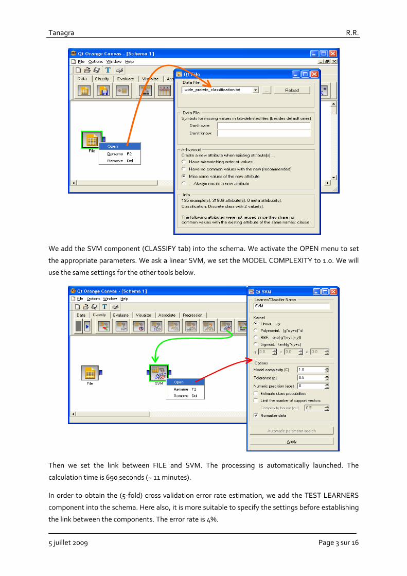
We add the SVM component (CLASSIFY tab) into the schema. We activate the OPEN menu to set

the appropriate parameters. We ask a linear SVM, we set the MODEL COMPLEXITY to 1.0. We will

use the same settings for the other tools below.

Then we set the link between FILE and SVM. The processing is automatically launched. The

calculation time is 690 seconds (~ 11 minutes).

In order to obtain the (5‐fold) cross validation error rate estimation, we add the TEST LEARNERS

component into the schema. Here also, it is more suitable to specify the settings before establishing

the link between the components. The error rate is 4%.

Tanagra R.R.


The peak of memory occupation during the whole process is 406 MB.

3.2 RAPIDMINER

The Java Virtual Machine is automatically started when we launch RAPIDMINER. The memory

occupation is 124 MB. After we create a new diagram, we insert the CSVEXAMPLESOURCE. The

settings must be specified with caution: FILENAME states the file name; LABEL_NAME states the

class attribute; we use a real with single precision for the data storage (DATAMANAGEMENT); the

COLUMN_SEPARATORS is tabulation. The processing time is 5 seconds. The memory occupation

becomes 210 MB.

Tanagra R.R.


RAPIDMINER supplies two components for SVM implementation. We test them in turns.

3.2.1 RAPIDMINER – JMYSVMLEARNER

The JMYSVMLEARNER component is a version of Stefan Ruping's MYSVM (http://www‐ai.cs.uni‐

dortmund.de/SOFTWARE/MYSVM/index.html). It is available into the menu item NEW OPERATOR

/ LEARNER / SUPERVISED / FUNCTIONS.

There are many parameters. Their consequence on the results seems not clear. We handle only the

complexity parameter (C = 1.0) and the kernel type (LINEAR).

We click on the PLAY button into the toolbar. The computation time is 29 seconds. The memory

occupation becomes 338 MB.

We implement a cross validation in order to measure the error rate.

Tanagra R.R.


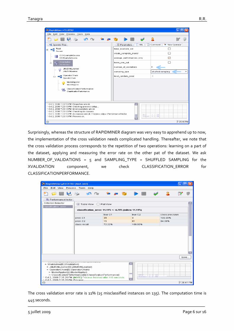
Surprisingly, whereas the structure of RAPIDMINER diagram was very easy to apprehend up to now,

the implementation of the cross validation needs complicated handling. Thereafter, we note that

the cross validation process corresponds to the repetition of two operations: learning on a part of

the dataset, applying and measuring the error rate on the other pat of the dataset. We ask

NUMBER_OF_VALIDATIONS = 5 and SAMPLING_TYPE = SHUFFLED SAMPLING for the

XVALIDATION component, we check CLASSIFICATION_ERROR for

CLASSIFICATIONPERFORMANCE.

The cross validation error rate is 11% (15 misclassified instances on 135). The computation time is

445 seconds.

Tanagra R.R.


3.2.2 RAPIDMINER – LIBSVM

A JAVA version of the famous library LIBSVM (http://www.csie.ntu.edu.tw/~cjlin/libsvm/) is available

into RAPIDMINER. We add the LIBSVMLEARNER component into the diagram. We set the

appropriate settings (KERNEL TYPE and C).

The real computation time is 9 seconds. But the listing of the coefficients of the linear classifier

takes more time. The memory occupation is 442 MB.

We obtain the cross validation error rate (2%, 3 misclassified instances) with the sequence of

components above. Curiously, the computation time is much longer here with 705 seconds. The

memory occupation is high: 870 MB.

Tanagra R.R.


3.3 TANAGRA

TANAGRA is intended to the Windows OS (W95 Vista). But it can launch on other OS using an

emulator or something like that (see http://data‐mining‐tutorials.blogspot.com/2009/01/tanagra‐

under‐linux.html for the utilization of Tanagra under Linux).

First of all, we click on the FILE / NEW menu in order to create a diagram and import the dataset. A

dialog box appears, we select the data file.

The importation time is 12 seconds. The enumeration of the variables into the visualization window

is longer. There are 31810 attributes (1 class attribute + 31809 descriptors) and 135 instances.

We specify the types of the variables using the DEFINE STATUS component. We set CLASSE as

TARGET, the other attributes as INPUT.

Tanagra R.R.


TANAGRA supplies two components for the implementation of SVM.

3.3.1 TANAGRA – SVM

The SVM component is a native implementation of the Platt’s SMO algorithm. We add it into the

diagram. We click on the PARAMETERS menu in order to set the appropriate settings.

The default settings are suitable. We click on the VIEW menu.

Tanagra R.R.


The calculation time is 130 seconds. It is rather high in comparison to other tools. We try to explain

why below (Section 3.5). The memory occupation is moderate (393 MB).

Then, we insert the CROSS VALIDATION component (SPV LEARNING ASSESSMENT tab). We

activate the PARAMETERS menu.

To launch the processing, we click on the VIEW menu. The error rate is 4% (6 misclassified

examples). During the calculations, the memory occupation remains stable (393 MB).

Tanagra R.R.


3.3.2 TANAGRA – LIBSVM

TANAGRA can use also the LIBSVM library (as DLL – Dynamic Link Library). We add the C‐SVC

component into the diagram. We click on the PARAMETERS menu. We use the default settings.

We click on the VIEW menu. The calculation is fast (11 seconds). Even if the dataset is duplicated

when we call the library, it seems it is not really detrimental since the memory occupation remains

reasonable (406 MB).

We implement the cross validation (5 FOLD). The obtained error rate is 4.44% (6 misclassified

instances). The calculation time is 64 seconds; the memory occupation remains stable (406 MB).

Tanagra R.R.


3.4 WEKA

The Java Virtual Machine is automatically launched with WEKA. We use the EXPLORER module in

this tutorial. We import the data by clicking on the OPEN FILE button with the CSVLOADER option.

The importation time is fast (10 seconds). The memory occupation reaches to 243 MB.

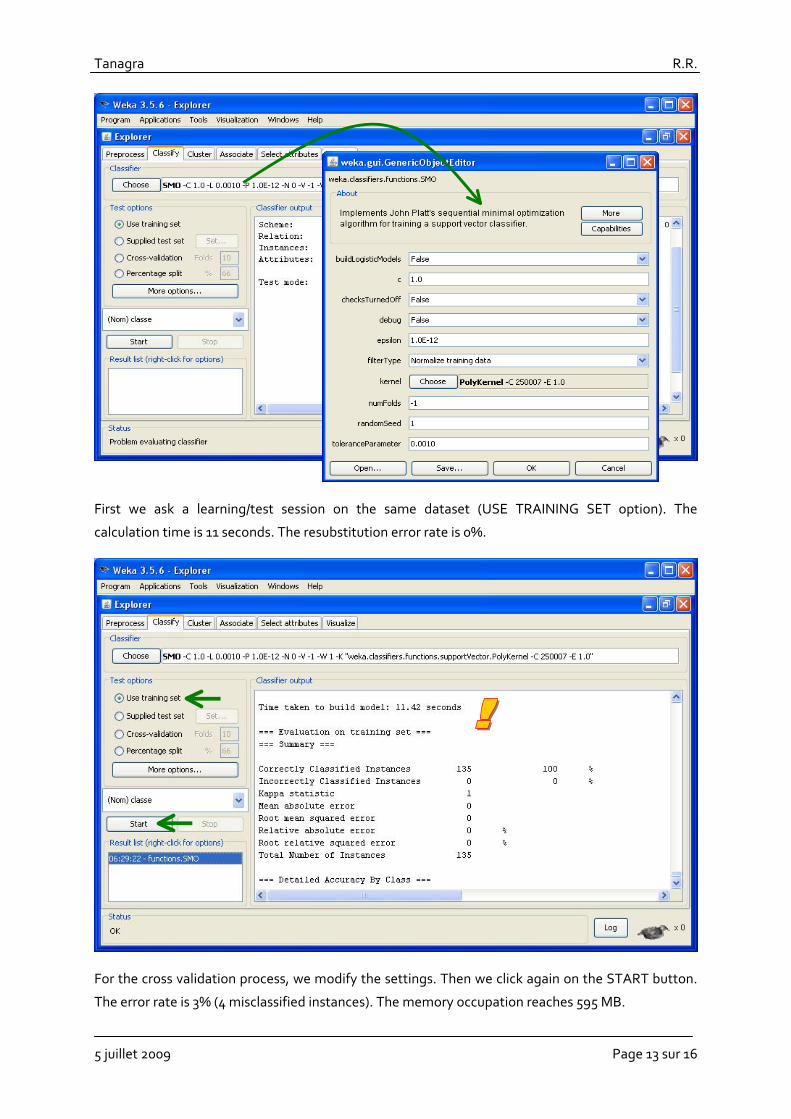
We activate the CLASSIFY tab. By clicking on the CHOOSE button, we select the SMO algorithm.

We can set the appropriate parameters i.e. we set C = 1.0 and a linear kernel (a polynomial kernel

with degree = 1).

Note: The LIBSVM library seems also available into WEKA. But on my computer, I cannot launch the

method. It seems the installation failed. The module was not reachable.

Tanagra R.R.


First we ask a learning/test session on the same dataset (USE TRAINING SET option). The

calculation time is 11 seconds. The resubstitution error rate is 0%.

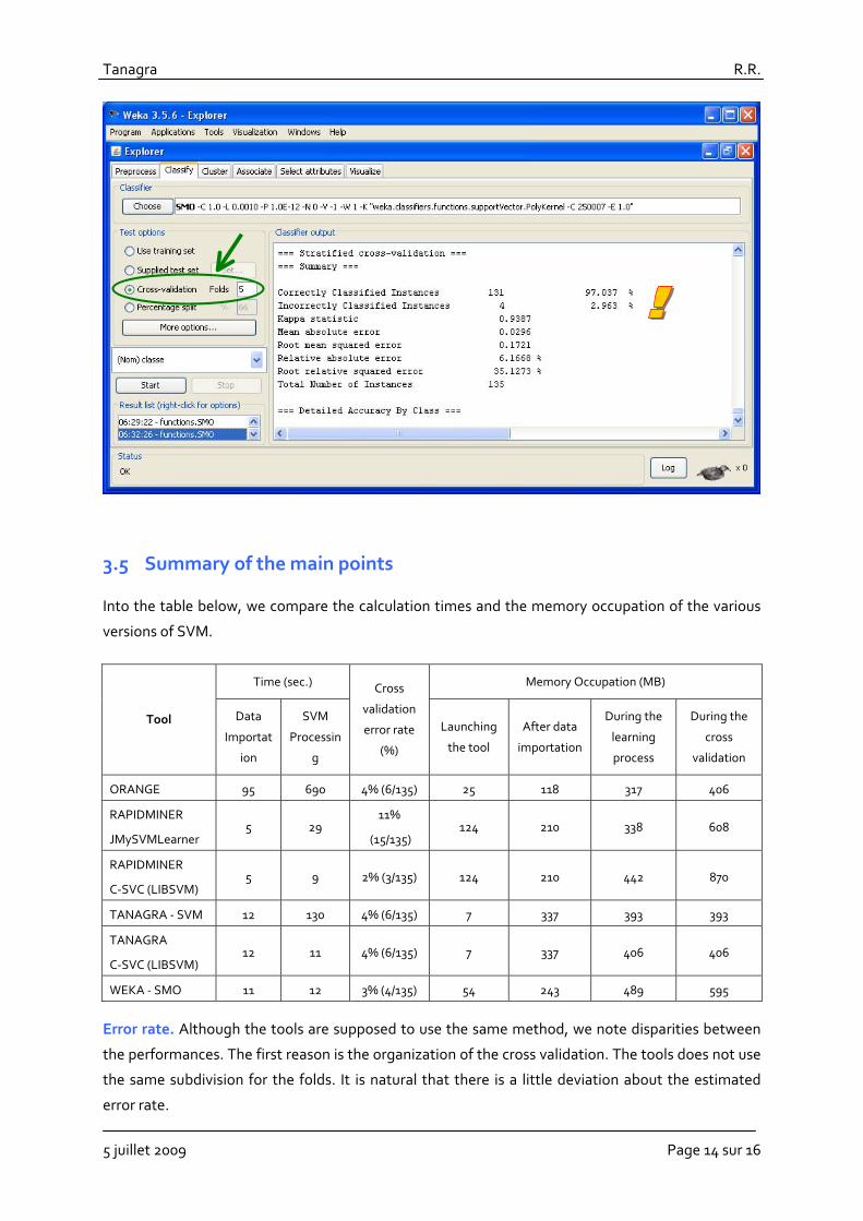
For the cross validation process, we modify the settings. Then we click again on the START button.

The error rate is 3% (4 misclassified instances). The memory occupation reaches 595 MB.

Tanagra R.R.


3.5 Summary of the main points

Into the table below, we compare the calculation times and the memory occupation of the various

versions of SVM.

Time (sec.) Memory Occupation (MB)

Tool Data

Importat

ion

SVM

Processin

g

Cross

validation

error rate

(%)

Launching

the tool

After data

importation

During the

learning

process

During the

cross

validation

ORANGE 95 690 4% (6/135) 25 118 317 406

RAPIDMINER

JMySVMLearner 5 29

11%

(15/135) 124 210 338 608

RAPIDMINER

C‐SVC (LIBSVM) 5 9 2% (3/135) 124 210 442 870

TANAGRA ‐ SVM 12 130 4% (6/135) 7 337 393 393

TANAGRA

C‐SVC (LIBSVM) 12 11 4% (6/135) 7 337 406 406

WEKA ‐ SMO 11 12 3% (4/135) 54 243 489 595

Error rate. Although the tools are supposed to use the same method, we note disparities between

the performances. The first reason is the organization of the cross validation. The tools does not use

the same subdivision for the folds. It is natural that there is a little deviation about the estimated

error rate.

Tanagra R.R.


The second reason is that the used algorithm is not the same one. That explains the strong

disparities in some circumstances. For example, JMYSVMLEARNER seems not efficient compared to

the others in the context of our data. It would be necessary to study in detail the algorithm and its

settings to understand this failure.

Processing time. I think that the LIBSVM library is extraordinary. Whatever tool in which it is

integrated, it is very fast. Into Tanagra, the data are duplicated before being sent to the compiled

library (DLL), this does not affect the processing time.

SMO of WEKA is also fast. Surprisingly, it is much faster than SMO of Tanagra while the source

codes are similar. After a thorough analysis of the stages of the algorithm, it seems that the

differences are primarily based on the data structure used. The dataset is organized by row into

Weka; they are organized by column into Tanagra. Thus, because SMO algorithm uses intensively a

dot product on row vector, Weka is much faster. In other contexts, when the calculations relies

mainly on analyzing the data by column (e.g. induction of decision trees), Tanagra is really more

efficient (http://data‐mining‐tutorials.blogspot.com/2008/11/decision‐tree‐and‐large‐dataset.html).

Morality of this, before you get excited unnecessarily on programming languages and compilers

(WEKA JAVA; TANAGRA DELPHI), we should first focus on the data structure when we want

to work on processing time.

Memory occupation. We note again here that JRE (Java Virtual Machine) leads to a more important

memory occupation, even if the internal data storage is efficient. We observe this by comparing the

memory occupation after the data loading and after the whole processing.

The behavior of RAPIDMINER‐LIBSVM during the cross‐validation suggests that many intermediate

results are kept, leading to unnecessary memory usage.

4 Related tools

We tested other tools. They failed at various step of the process. The reasons are not clear

sometimes.

• KNIME (1.5.31 ‐ http://www.knime.org/): It was not possible to import data. During the

preview, the software crashes. It seems that this is due to the visualization grid. There is no

reason that the internal structures cannot handle the data.

• R (package e1071 ‐ http://cran.r‐project.org/web/packages/e1071/index.html): We use

the package “e1071” of R 2.7.2 (http://www.r‐project.org/). The data file is rightly imported.

The loading time is 35 seconds. The memory occupation is grown from 19 MB to 156 MB.

The problem occurs when we launch the SVM. R tries to create a vector of 3.8 GB size. It is

not possible on my computer. I do not think it is possible under Windows OS. Furthermore,

this value (3.8 GB) seems mysterious.

Tanagra R.R.


• Many libraries are available online (e.g. http://www.support‐vector‐

machines.org/SVM_soft.html). The main difficulty is to prepare the data in the correct

format in order to launch the tool. Some libraries are associated with commercial software

such as MATLAB, their diffusion is necessarily limited.

5 Conclusion

In drawing a parallel between this tutorial and this one dedicated to the induction of decision trees

on large databases (http://data‐mining‐tutorials.blogspot.com/2008/11/decision‐tree‐and‐large‐

dataset.html), we realize that the solutions are more or less efficient depending on the

characteristics of data handled and the learning method used. This confirms the idea that there is no

universal solution. We must determine the most appropriate solution depending on the context of

the study that we conducted.

Anyone can reproduce the experiment described in this tutorial. We can also lead the experiment on

a dataset with other characteristics (e.g. many rows, few columns). The conclusions can be different

in this context.

tanagra perfs comp svm -...

Documents