technical report - 株式会社qt · this tr describes the physical layer aspect of the techniques...

3GPP TR 25.848 V4.0.0(2001-03)Technical Report

3rd Generation Partnership Project;Technical Specification Group Radio Access Network;

Physical layer aspects of UTRA High Speed Downlink PacketAccess

(Release 4)

The present document has been developed within the 3rd Generation Partnership Project (3GPP TM) and may be further elaborated for the purposes of 3GPP. The present document has not been subject to any approval process by the 3GPP Organisational Partners and shall not be implemented. This Specification is provided for future development work within 3GPP only. The Organisational Partners accept no liability for any use of this Specification.Specifications and reports for implementation of the 3GPP TM system should be obtained via the 3GPP Organisational Partners' Publications Offices.

3GPP

3GPP TR 25.848 V4.0.0(2001-03)2Release 4

Keywords UMTS, radio, packet mode, layer 1

3GPP

Postal address

3GPP support office address 650 Route des Lucioles - Sophia Antipolis

Valbonne - FRANCE Tel.: +33 4 92 94 42 00 Fax: +33 4 93 65 47 16

Internet http://www.3gpp.org

Copyright Notification

No part may be reproduced except as authorized by written permission. The copyright and the foregoing restriction extend to reproduction in all media.

© 2001, 3GPP Organizational Partners (ARIB, CWTS, ETSI, T1, TTA,TTC).

All rights reserved.

3GPP

3GPP TR 25.848 V4.0.0(2001-03)3Release 4

Contents Foreword ............................................................................................................................................................6 1 Scope ........................................................................................................................................................7 2 References ................................................................................................................................................7 3 Definitions, symbols and abbreviations ...................................................................................................7 4 Background and Introduction...................................................................................................................7 5 Overview oftTechnologies considered to support UTRA High Speed Downlink Packet Access ...........7 Adaptive Modulation and Coding (AMC).......................................................................................................................... 7 5.1 Hybrid ARQ (H-ARQ)............................................................................................................................................ 8 5.2 Fast Cell Selection (FCS) ........................................................................................................................................ 9 5.3 Multiple Input Multiple Output Antenna Processing .............................................................................................. 9 5.4 Stand-Alone DSCH ............................................................................................................................................... 10 6 Proposed physical layer structure of High Speed Downlink Packet Access.........................................10 6.1 Basic Physical Structure <frame length, update rates spreading codes, etc>......................................... 10 6.1.1 HSDPA physical-layer structure in the code domain....................................................................................... 10 6.1.2 HSDPA physical-layer structure in the time domain ....................................................................................... 11 6.2 Adaptive Modulation and Coding (AMC)............................................................................................................. 12 6.3 Hybrid ARQ (H-ARQ).......................................................................................................................................... 12 6.4 Fast Cell Selection (FCS) ...................................................................................................................................... 14 6.4.1 Physical-layer measurements for cell selection in case of fast cell selection................................................... 15 6.4.2 Physical-layer signalling for cell selection in case of fast cell selection.......................................................... 15 6.4.3 Physical-layer signalling for transmission-state synchronisation in case of inter-Node-B FCS ...................... 15 6.4.4 Conclusions...................................................................................................................................................... 15 6.5 Multiple input multiple output antenna processing ............................................................................................... 16 6.6 Associated signaling needed for operation of High Speed Downlink Packet Access .......................................... 18 6.6.1 Associated Uplink signaling ............................................................................................................................ 18 6.6.2 Associated Downlink signaling ....................................................................................................................... 18 6.7 Evaluation of technologies .....................................................................................................................19 6.7 Adaptive Modulation and Coding (AMC)............................................................................................................. 19 6.7.1 Performance Evaluation <throughput, delay> ................................................................................................. 19 6.7.2 Complexity Evaluation <UE and RNS impacts>............................................................................................. 22 6.7.3 Complexity Impacts to UE .............................................................................................................................. 22 6.7.3.1 Introduction...................................................................................................................................................... 22 6.7.3.2 Detection of MCS applied by Node-B............................................................................................................. 22 6.7.3.3 Demodulation of higher order modulation....................................................................................................... 22 6.7.3.4 Decoding of turbo code.................................................................................................................................... 23 6.7.3.5 Measurement/Reporting of downlink channel quality ..................................................................................... 24 6.7.3.6 Conclusions...................................................................................................................................................... 24 6.7.4 Advanced Technologies................................................................................................................................... 24 6.7.4.1 Interference Canceller and Equalizers for Higher Modulation ........................................................................ 24 6.7.5 Complexity Impacts to RNS ............................................................................................................................ 26 6.8 Hybrid ARQ (H-ARQ).......................................................................................................................................... 26 6.8.1 Performance Evaluation <throughput, delay> ................................................................................................. 26 6.8.1.1 Link Performance Comparison of Type-II and Type III HARQ Schemes ...................................................... 26 6.8.2 Summary for CPICH SIR errors w/wo H-ARQ based on System Simulations:.............................................. 31 6.8.2.1 CPICH SIR Measurement Error model ........................................................................................................... 31 6.8.2.2 Hybrid ARQ (Chase combining) modeling ..................................................................................................... 31 6.8.2.3 Simulation Results/Conclusions for CPICH SIR errors w/wo H-ARQ ........................................................... 32 6.8.3 Complexity Evaluation <UE and RNS impacts>............................................................................................. 35 6.8.3.1 N-channel stop-and-wait H-ARQ .................................................................................................................... 35 6.8.3.1.1 Introduction................................................................................................................................................ 35 6.8.3.1.2 Buffering complexity ................................................................................................................................. 35 6.8.3.1.3 Encoding/decoding and rate matching complexity .................................................................................... 38

3GPP

3GPP TR 25.848 V4.0.0(2001-03)4Release 4

6.8.3.1.4 UE and RNS processing time considerations............................................................................................. 38 6.8.3.1.5 Conclusions................................................................................................................................................ 41 6.9 Fast Cell Selection (FCS) ...................................................................................................................................... 41 6.9.1 Performance Evaluation <throughput, delay> ................................................................................................. 41 6.9.1.1 Summary for FCS benefit: ............................................................................................................................... 41 6.9.1.2 Conclusion for FCS benefit: ............................................................................................................................ 41 6.9.1.3 FCS function description ................................................................................................................................. 41 6.9.2 Complexity Evaluation <UE and RNS impacts>............................................................................................. 45 6.10 Multiple input multiple output antenna processing.......................................................................................... 45 6.10.1 MIMO performance evaluation ....................................................................................................................... 45 6.10.2 MIMO UE complexity evaluation ................................................................................................................... 49 6.10.3 Node-B Complexity Evaluation....................................................................................................................... 49 7 Physical layer aspects for TDD mode ....................................................................................................49 7.1 Techniques to support HSDPA for TDD mode..................................................................................................... 49 7.1.1 Adaptive Modulation and Coding.................................................................................................................... 50 7.1.2 Hybrid ARQ (H-ARQ) .................................................................................................................................... 50 7.1.3 Fast Cell Selection (FCS) ................................................................................................................................ 51 7.1.4 MIMO.............................................................................................................................................................. 51 7.2 Simulation assumptions......................................................................................................................................... 51 7.3 Link-level simulation results ................................................................................................................................. 51 8 Backwards compatibility aspects ...........................................................................................................53 9 Conclusions and recommendations........................................................................................................53

Annex A: Simulation Assumptions and Results ..................................................................................54 A.1 Link simulation assumptions..................................................................................................................54 A.1.1 Link assumptions ............................................................................................................................................. 54 A.1.2 Simulation description overview ..................................................................................................................... 54 A.1.3 Standard constellations for m-ary modulation ................................................................................................. 54 A.1.4 Turbo decoding................................................................................................................................................ 56 A.1.5 Other decoding................................................................................................................................................. 57 A.1.6 Performance metrics: ....................................................................................................................................... 57 A.1.7 Simulation Parameters: .................................................................................................................................... 58 A.1.8 Simulation cases .............................................................................................................................................. 60 A.2 Link simulation results ...........................................................................................................................60 A.2.1 Effect of multipath ........................................................................................................................................... 65 A.2.2 Effect of non-ideal channel estimation: ........................................................................................................... 65 A.3 System simulation assumptions .............................................................................................................67 A.3.1 Common system level simulation assumptions ............................................................................................... 68 A.3.2 Basic system level parameters ......................................................................................................................... 68 A.3.3 Data traffic model ............................................................................................................................................ 68 A.3.4 UE mobility model........................................................................................................................................... 69 A.3.5 Packet scheduler .............................................................................................................................................. 69 A.3.6 Outputs and performance metrics .................................................................................................................... 70 A.3.7 Simulation cases .............................................................................................................................................. 71 A.3.7.1 Case 1 .............................................................................................................................................................. 71 A.3.7.2 Case 2 .............................................................................................................................................................. 71 A.4 System simulation results.......................................................................................................................72 A.4.1 HSDPA baseline performance (AMC, HARQ, FCS, Fast Scheduler, 3,33ms frame) vs Release 99

Bound............................................................................................................................................................... 72 A.4.2 Sensitivity to propagation exponent................................................................................................................. 74 A.4.3 Effects of non-ideal measurement and feedback ............................................................................................. 75 A.4.4 Effect of MCS selection delay on the performance of HSDPA....................................................................... 76 A.4.5 Integrated voice and data performance ............................................................................................................ 78 A.4.6 Control information delay................................................................................................................................ 82

3GPP

3GPP TR 25.848 V4.0.0(2001-03)5Release 4

Annex B: Examples of Performance Evaluation methods .................................................................85

Annex C: Throughput Metric Definitions ...........................................................................................87

Annex D: Change history ......................................................................................................................89

3GPP

3GPP TR 25.848 V4.0.0(2001-03)6Release 4

Foreword This Technical Specification has been produced by the 3rd Generation Partnership Project (3GPP).

The contents of the present document are subject to continuing work within the TSG and may change following formal TSG approval. Should the TSG modify the contents of the present document, it will be re-released by the TSG with an identifying change of release date and an increase in version number as follows:

Version x.y.z

where:

x the first digit:

1 presented to TSG for information;

2 presented to TSG for approval;

3 or greater indicates TSG approved document under change control.

y the second digit is incremented for all changes of substance, i.e. technical enhancements, corrections, updates, etc.

z the third digit is incremented when editorial only changes have been incorporated in the document.

3GPP

3GPP TR 25.848 V4.0.0(2001-03)7Release 4

1 Scope This TR describes the physical layer aspect of the techniques behind the concept of high-speed downlink packet access (HSDPA). Furthermore, it also reports the performance and complexity evaluation of the HSDPA, done for the HSDPA feasibility study.

2 References The following documents contain provisions which, through reference in this text, constitute provisions of the present document.

• References are either specific (identified by date of publication, edition number, version number, etc.) or non-specific.

• For a specific reference, subsequent revisions do not apply.

• For a non-specific reference, the latest version applies. In the case of a reference to a 3GPP document (including a GSM document), a non-specific reference implicitly refers to the latest version of that document in the same Release as the present document.

[1] 3GPP TS 25.123: "Example 1, using sequence field".

[2] 3GPP TR 29.456 (V3.1.0): "Example 2, using fixed text".

3 Definitions, symbols and abbreviations (void)

4 Background and Introduction The study item HSDPA studies enhancements that can be applied to UTRA in order to provide very high speed downlink packet access by means of a high-speed downlink shared channel (HS-DSCH).

5 Overview oftTechnologies considered to support UTRA High Speed Downlink Packet Access

Adaptive Modulation and Coding (AMC) The benefits of adapting the transmission parameters in a wireless system to the changing channel conditions are well known. In fact fast power control is an example of a technique implemented to enable reliable communications while simultaneously improving system capacity. The process of modifying the transmission parameters to compensate for the variations in channel conditions is known as link adaptation. Another technique that falls under this category of link adaptation, is adaptive modulation and coding (AMC).

The principle of AMC is to change the modulation and coding format in accordance with variations in the channel conditions, subject to system restrictions. The channel conditions can be estimated e.g. based on feedback from the receiver In a system with AMC, users in favorable positions e.g. users close to the cell site are typically assigned higher order modulation with higher code rates (e.g. 64 QAM with R=3/4 Turbo Codes), while users in unfavorable positions e.g. users close to the cell boundary, are assigned lower order modulation with lower code rates (e.g. QPSK with R=1/2 Turbo Codes). The main benefits of AMC are, a) higher data rates are available for users in favorable positions which in turn increases the average throughput of the cell and b) reduced interference variation due to link adaptation based on variations in the modulation/coding scheme instead of variations in transmit power.

3GPP

3GPP TR 25.848 V4.0.0(2001-03)8Release 4

AMC is also effective when combined with fat-pipe scheduling techniques such as those enabled by the Downlink Shared Channel. On top of the benefits attributed to fat-pipe multiplexing [2], AMC combined with time domain scheduling offers the opportunity to take advantage of short term variations in a UE’s fading envelope so that a UE is always being served on a constructive fade. Figure 1 shows the Rayleigh fading envelope correlation vs. time delay for different values of Doppler frequency. The figure suggests that for lower Doppler frequencies it is possible to schedule a user on a constructive fade provided that the scheduling interval (i.e. frame size) is small and the measurement reports are timely (i.e. distributed scheduling).

Envelope Correlation

0

0.1

0.2

0.3

0.4

0.5

0.6

0.7

0.8

0.9

1

0 5 10 15 20 25 30

Time (msec)

Cor

rela

tion

fd=5Hz fd=10Hz fd=30Hz fd=50Hz

Figure 1. Envelope Correlation as a function of different doppler

5.1 Hybrid ARQ (H-ARQ) H-ARQ is an implicit link adaptation technique. Whereas, in AMC explicit C/I measurements or similar measurements are used to set the modulation and coding format, in H-ARQ, link layer acknowledgements are used for re-transmission decisions. There are many schemes for implementing H-ARQ - Chase combining, Rate compatible Punctured Turbo codes and Incremental Redundancy. Incremental redundancy or H-ARQ-type-II is another implementation of the H-ARQ technique wherein instead of sending simple repeats of the entire coded packet, additional redundant information is incrementally transmitted if the decoding fails on the first attempt.

H-ARQ-type-III also belongs to the class of incremental redundancy ARQ schemes. However, with H-ARQ-type-III, each retransmission is self-decodable which is not the case with H-ARQ-type II. Chase combining (also called H-ARQ-type-III with one redundancy version) involves the retransmission by the transmitter of the same coded data packet. The decoder at the receiver combines these multiple copies of the transmitted packet weighted by the received SNR. Diversity (time) gain is thus obtained. In the H-ARQ-type-III with multiple redundancy version different puncture bits are used in each retransmission.

AMC by itself does provide some flexibility to choose an appropriate MCS for the channel conditions based on measurements either based on UE measurement reports or network determined. However, an accurate measurement is required and there is an effect of delay. Also, an ARQ mechanism is still required. H-ARQ autonomously adapts to the instantaneous channel conditions and is insensitive to the measurement error and delay. Combining AMC with H-ARQ leads to the best of both worlds - AMC provides the coarse data rate selection, while H-ARQ provides for fine data rate adjustment based on channel conditions.

The choice of H-ARQ mechanism however is important. Window based Selective Repeat (SR) is a common type of ARQ protocol employed by many systems including RLC R99. SR is generally insensitive to delay and has the favorable property of repeating only those blocks that have been received in error. To accomplish this feat, the SR ARQ transmitter must employ a sequence number to identify each block it sends. SR may fully utilize the available channel

3GPP

3GPP TR 25.848 V4.0.0(2001-03)9Release 4

capacity by ensuring that the maximum block sequence number (MBSN) exceeds the number of blocks transmitted in one round trip feedback delay. The greater the feedback delay the larger the maximum sequence number must be. However, when Hybrid ARQ is partnered with SR, several difficulties are seen.

• UE memory requirements are high. The mobile must store soft samples for each transmission of a block. MSBN blocks may be in transit at any time. A large MBSN requires significant storage in the UE adding to the unit’s cost.

• Hybrid ARQ requires the receiver to reliably determine the sequence number of each transmission. Unlike conventional ARQ, every block is used even if there is an error in the data. In addition, the sequence information must be very reliable to overcome whatever channel conditions have induced errors in the data. Typically a separate, strong code must be used to encode the sequence information, effectively multiplying the bandwidth required for signaling

Stop-and-wait is one of the simplest forms of ARQ requiring very little overhead. In stop-and-wait, the transmitter operates on the current block until the block has been received successfully. Protocol correctness is ensured with a simple one-bit sequence number that identifies the current or the next block. As a result, the control overhead is minimal. Acknowledgement overhead is also minimal, as the indication of a successful/unsuccessful decoding (using ACK, NACK, etc) may be signaled concisely with a single bit. Furthermore, because only a single block is in transit at a time, memory requirements at the UE are also minimized. Therefore, HARQ using a stop-and-wait mechanism offers significant improvements by reducing the overall bandwidth required for signaling and the UE memory. However, one major drawback exists: acknowledgements are not instantaneous and therefore after every transmission, the transmitter must wait to receive the acknowledgement prior to transmitting the next block. This is a well-known problem with stop-and-wait ARQ. In the interim, the channel remains idle and system capacity goes wasted. In a slotted system, the feedback delay will waste at least half the system capacity while the transmitter is waiting for acknowledgments. As a result, at least every other timeslot must go idle even on an error free channel.

N channel stop-and-wait Hybrid ARQ offers a solution by parallelizing the stop-and-wait protocol and in effect running a separate instantiation of the Hybrid ARQ protocol when the channel is idle. As a result no system capacity goes wasted since one instance of the algorithm communicates a data block on the forward link at the same time that the other communicates an acknowledgment on the reverse link. However, the receiver has to store N blocks for this scheme.

5.2 Fast Cell Selection (FCS) Fast Cell Selection (FCS) has been proposed for HSDPA. Using FCS, the UE indicates the best cell which should serve it on the downlink, through uplink signaling. Thus while multiple cells may be members of the active set, only one of them transmits at any time, potentially decreasing interference and increasing system capacity.

5.3 Multiple Input Multiple Output Antenna Processing Diversity techniques based on the use of multiple downlink transmit antennas are well known; second order applications of these have been applied in the UTRA Release 99 specifications. Such techniques exploit spatial and/or polarisation decorrelations over multiple channels to achieve fading diversity gains.

Multiple input multiple output (MIMO) processing employs multiple antennas at both the base station transmitter and terminal receiver, providing several advantages over transmit diversity techniques with multiple antennas only at the transmitter and over conventional single antenna systems. If multiple antennas are available at both the transmitter and receiver, the peak throughput can be increased using a technique known as code re-use. With code re-use, each channelization/scrambling code pair allocated for HS-DSCH transmission can modulate up to M distinct data streams, where M is the number of transmit antennas. Data streams which share the same channelization/scrambling code must be distinguished based on their spatial characteristics, requiring a receiver with at least M antennas. In principle, the peak throughput with code re-use is M times the rate achievable with a single transmit antenna. Third, with code re-use, some intermediate data rates can be achieved with a combination of code re-use and smaller modulation constellations e.g. 16 QAM instead of 64 QAM. Compared to the single antenna transmission scheme with a larger modulation constellation to achieve the same rate, the code re-use technique may have a smaller required Eb/No, resulting in overall improved system performance. The technique discussed so far is an open-loop technique since the Node B transmitter does not require feedback from the UE other than the conventional HSDPA information required for rate determination. Further performance gains can be achieved using closed-loop MIMO techniques whereby the Node B transmitter employs feedback information from the UE. For example, with knowledge of channel realizations, the Node B could transmit on orthogonal eigenmodes, eliminating the spatial multi-access interference.

3GPP

3GPP TR 25.848 V4.0.0(2001-03)10Release 4

5.4 Stand-Alone DSCH A stand-alone DSCH is defined as a DSCH or a HS-DSCH mapped on a downlink carrier that is different from the carrier that supports its associated DCH/DPCH as documented in 25.950, the RAN 2 TR on HSDPA.

The stand-alone DSCH may be seen as a specific case of mapping of the transport channels set up on the downlink to a UE in a multi-carrier cell. The multi-carrier cell concept may correspond to several cases: cells with a possibly asymmetrical number of carriers up and downlink and cells with carriers which are part of different bands, these two cases being possibly combined.

The introduction of the Stand-alone DSCH would lead to some modifications of the physical layer structure as far as physical channel characteristics are concerned. Impact is mostly on the UE, as a double receiver would be needed due to the simultaneous reception on two carriers. Note that, if the UE would include such a second receiver, it could also be used for IF measurements, thus reducing the need for Compressed Mode depending on the band used.

The signalling for stand-alone DSCH will be carried on the carrier that supports its associated DCH/DPCH. Due to strict asymmetric nature of the stand-alone DSCH, the signalling impact on the carrier that carries the companion DCH will also be asymmetric that can lead to limitations in resource allocation to symmetric services.

The introduction of independence between the frequency carrier supporting the DCH and the carrier supporting the stand-alone DSCH corresponds to an added flexibility with respect to R99 DSCH and HS-DSCH for which the DCH and DSCH/HS-DSCH are mapped onto the same carrier. It allows to segregate transport channels for the same UE with different QoS requirements onto different carriers. By assigning up to whole carrier for the HS-DSCH, the maximum power and code space available for HS-DSCH transmission would be increased as no resource has to be set aside for DCH or common channels. This would in turn allow for HS-DSCH transmission with higher peak rates.

6 Proposed physical layer structure of High Speed Downlink Packet Access

6.1 Basic Physical Structure <frame length, update rates spreading codes, etc> On the physical layer, HSDPA transmission should be carried out on a set of downlink physical channels (codes) shared by users at least in the time domain and possibly also in the code domain.

6.1.1 HSDPA physical-layer structure in the code domain In terms of physical channel structure and the HS-DSCH mapping to physical channels (codes), different alternatives with different levels of flexibility have been discussed within RAN1:

Alternative 1

The same level of high flexibility as for release 99 DSCH transmission implying that the physical channels to which HS-DSCH is mapped are shared between “users” in the time domain ("time multiplex") as well as in the code domain ("code multiplex") the physical channels to which HS-DSCH is used may have different spreading factors

Alternative 2

The physical channels to which HS-DSCH is mapped has a fixed spreading factor, as shown in Figure 2. The selection of such a fixed HSDPA spreading factor should be based on an evaluation of the impact on

- Performance

- UE complexity

- Flexibility (granularity in the overall allocation of capacity for HSDPA transmission)

The physical channels to which HS-DSCH is mapped can still be shared between “users” in the time domain as well as in the code domain, as shown in

3GPP

3GPP TR 25.848 V4.0.0(2001-03)11Release 4

Figure 3. Physical layer block diagram conceptually showing the transmit chain for this approach is shown in Figure 4. It may be noted that link level simulations were performed based on Figure 4.

SF=8

SF=16

SF=4

SF=2

SF=1

Physical channels (codes) to which HS-DSCH is mapped

SFHSDPA = 16 (example)Number of codes to which HSDPA transmission is mapped: 12 (example)

Figure 2. HSDPA mapping to physical channels with fixed spreading factor

All codes to whichHSDPA transmissionis mapped(5 in this example)

Data to UE #1 Data to UE #2 Data to UE #3 CodeCode

Time

Figure 3. Sharing by means of time multiplex as well as code multiplex

TailBits

TurboEncoder

RateMatching Interleave

QPSK/8-PSK/M-QAM

AMCS

DEMUX

W SFM

W SF1

. .

..

. .

Σ

N TransportBlocks

Figure 4. HSDPA Physical Layer Structure

6.1.2 HSDPA physical-layer structure in the time domain In the time domain, the support of HSDPA TTI shorter than one radio frame (10 ms) has been proposed. The length of such shorter HSDPA TTI should be selected from the set {Tslot, 3×Tslot, 5×Tslot, 15×Tslot}. The selection of such shorter HSDPA TTI should be based on an evaluation of the impact on

- Performance

- Delay

3GPP

3GPP TR 25.848 V4.0.0(2001-03)12Release 4

- Network and UE complexity

- Flexibility (HSDPA payload granularity)

Two approaches have been identified for Transmission Time Interval in HS-DSCH: an approach with fixed TTI and the second approach of dynamic TTI [1]. With the variable TTI approach, the duration of the transmission is varied while the code block size in bits is kept fixed.

Variable TTI adds flexibility in resource allocation in the time domain in addition to the flexibility that exists in code domain for fixed TTI. Variable TTI is well suited for fat-pipe scheduling techniques such as those enabled by the Downlink Shared Channel. Variable TTI schemes should be compared to schemes that use fixed TTIs in terms of performance, flexibility and complexity.

6.2 Adaptive Modulation and Coding (AMC) The implementation of AMC offers several challenges. First, AMC is sensitive to measurement error and delay. In order to select the appropriate modulation, the scheduler must be aware of the channel quality. Errors in the channel estimate will cause the scheduler to select the wrong data rate and either transmit at too high a power, wasting system capacity, or too low a power, raising the block error rate. Delay in reporting channel measurements also reduces the reliability of the channel quality estimate due to the constantly varying mobile channel. Furthermore changes in the interference add to the measurement errors. Hybrid ARQ (HARQ) enables the implementation of AMC by reducing the number of required MCS levels and the sensitivity to measurement error and traffic fluctuations.

There are different methods by which the HS-DSCH transport format can be selected. These options are not mutually exclusive:

a.)The UE may estimate/predict the downlink channel quality and calculate a suitable transport format that is reported to the Node-B

b.)The UE may estimate/predict the downlink channel quality and report this to the Node-B.

c) Node-B may determine the transport format without feedback from the UE e.g. based on power control gain of the associated dedicated physical channel.

6.3 Hybrid ARQ (H-ARQ) In order to reduce receiver buffering requirements a HARQ scheme based on N-channel stop-and-wait protocol has been proposed. There are two different methods for N-channel HARQ:

a) either signal the subchannel number explicitely (fully asynchronous), or

b) tie the subchannel number to e.g. frame timing (partially asynchronous).

Method a) is illustrated in the Figure 5 which shows an example sequence of events when packets 1-7 are being transmitted to UE1 and packet 1 to UE2 using N-channel HARQ with N=4 and 3 slot TTI. Packets are transmitted using four parallel ARQ processes for UE1 and one ARQ process for UE2, each using stop-and-wait principle. Each packet is acknowledged during the transmission of other packets so that the downlink channel can be kept occupied all the time if there are packets to transmit.

3GPP

3GPP TR 25.848 V4.0.0(2001-03)13Release 4

HSPDSCH1 UE1 Packet 1UE1 packet 2

Node B1

UE1 Packet 3UE1 Packet 4UE2 Packet 1UE1 Packet 5UE1 packet 2UE1 Packet 6UE1 Packet 4

UL DPCCH UE1

UL DPCCH UE2

A N A N A A A A A

A

UE1 Packet 7UE2 Packet 2

UE1 HARQ channel 1 UE1 HARQ channel 2 UE1 HARQ channel 3 UE1 HARQ channel 4

UE2 HARQ channel 1

Figure 5. Principle of N-channel stop-and-wait HARQ (N=4).

N-channel HARQ supports asynchronous transmission: different users can be scheduled freely without waiting completion of a given transmission (Receiver needs to know which HARQ process the packet belongs to, which can be explicitly signaled on HSDPA control channel.). The transmission for a given user is assumed to continue when the channel is again allocated. The asynchronous feature of N-channel HARQ is also shown in Figure 1: after four packets to UE1, a packet is transmitted to UE2 and the transmission to UE1 is delayed by one TTI. Also, there are 5 packets to UE1 between packets to UE2. The processing times should be defined such that continuous transmission to a UE is possible.

Method b) would restrict the positions of retransmissions such that the retransmissions can only happen at positions m+k*N, where m is the position (TTI) of the first transmission of a given packet and k = 1,2,…. The retransmissions could still be delayed if the channel is allocated to other users in between.

There are a number of issues that need to be studied and specified if N channel HARQ will be used including:

- Downlink signaling requirements

- Uplink signaling requirements

- Coding solution

- UE and Node B processing requirements

- Max number of parallel ARQ processes

- Max number of retransmissions

- Interaction with AMC and FCS

For each HSDPA TTI, receiver needs to know which HARQ process (subchannel) the transport block(s) of that TTI belong to. As explained earlier there are two methods: a) that could be explicitly signaled requiring log

2(N) bits per

HSDPA TTI or b) deterministic mapping between the ARQ processes and e.g. CFN could be defined allowing the receiver to distinguish which one of the N channels is being received in a given HSDPA TTI,thus requiring no signaling.

It could also be useful to signal in downlink the redundancy version of the transport block(s) received during a HSDPA TTI. In most simple case this could be just a indication of a start of a new packet (i.e. RLC PDU). This would aid the receiver to perform the combining and decoding of the transport block(s) properly in case of signaling errors in uplink. If incremental redundancy schemes are used even the redundancy version could be signaled to the UE requiring at least log

2(# of redundancy versions) bits per HSDPA TTI.

In the uplink direction acknowledgements of the received RLC PDUs are sent. In a straightforward solution this would require 1 bit per received HSDPA TTI to be transmitted from UE to Node B. If there are more than one transport block in a HSDPA TTI, they could be acknowledged individually resulting in higher uplink signaling load but possible better link performance. However, it is understood by RAN WG1 that when the HSDPA TTI is in error, the majority of the transport blocks within it are also erroneous.Thus, it is desirable to retransmit the whole TTI.

3GPP

3GPP TR 25.848 V4.0.0(2001-03)14Release 4

An important issue is the encoding solution of the HARQ, i.e. if Type II or Type III HARQ will be used. A simple solution is to use Type III with single redundancy version meaning that received code blocks are simply soft combined before decoding. In case of Type II or Type III with multiple redundancy versions, additional redundancy bits are sent during each retransmission yielding potentially more coding gain than simple Type III with single redundancy version. Which scheme will be adopted should be based on performance improvement and complexity considerations.

In order to reduce the UE’s buffer size for Type-III H-ARQ with multiple redundancy versions, Separate Systematic and Parity information Mapping (SSPM) may be employed. In this concept Node B maps systematic information and parity information on separate symbols. UE combines systematic information of all received packets in symbol domain before calculating Log Likelihood Ratio.

Due to strict timing requirements of N channel stop-and-wait HARQ scheme the processing time requirements both in UE and Node B should be carefully studied. At UE side there should be sufficient time left for all the processing after the reception of the transport blocks of a HSDPA TTI until the transmission of acknowledgement in uplink. Similarly, sufficient time should be left for Node B to react to the received acknowledgement message before the next transmission time interval for the given HARQ process.

Figure 5 also shows an example of a feedback timing of a 4-channel stop-and-wait HARQ. In this case 3 slot HSDPA TTI has been assumed. HARQ feedback is transmitted over one uplink slot leaving at least 3 slots time for processing both in UE and Node B.

For a fixed HSDPA TTI length, increasing the number (N) of parallel HARQ processes will improve the time diversity per process and could result in longer available processing times both at UE and Node B. Downside include the increased buffering requirements at UE, longer delay per process and higher uplink signaling load in case the HARQ state information need to be communicated to new Node B while doing FCS. These factors should be taken into account when defining the maximum for N. Note that for very short (< 3 slots) HSDPA TTI it could be beneficial to have N always greater than 2 because then, for example, the processing time requirements would not be too demanding.

Maximum number of retransmissions could be fixed to a constant value or it could be a parameter whose value can be set based on various criteria. Defining it as a parameter would mean a bit more flexibility in controlling the delay characteristics over the air interface. Note that if some indication of the start of a new RLC PDU is send to UE it is not absolutely necessary for UE to know what is the maximum allowed number of retransmissions. Yet, due to signaling errors it is probably beneficial to negotiate that information between the network and UE in order to recover faster from erroneous situations.

When N-channel HARQ is used in addition to other proposed performance enhancement techniques like AMC and FCS there are certain interactions between them that need to be considered. One example of interaction is the choice of MCS for retransmission. The choice of MCS for retransmission could be the same as that of the original transmission (fixed) or could be allowed to change (adaptive). If the delay between the original transmission and retransmission is long, the MCS level supportable to the user at the time of retransmission may be different. The change in the supportable MCS level to the user may be due to change in the channel conditions, available power and/or codes for HS-DSCH.

When FCS is applied it is probable that HARQ state information needs to be communicated to a new Node B. In order to minimize this signaling load in the uplink, the number of parallel HARQ processes should be kept small. This should be taken into consideration when defining the maximum value of N. At the time of cell selection, it is possible that some of the HARQ channels are pending recovery. Here again there is interaction between HARQ and AMC in terms of whether retransmissions need to be at the same MCS level or not. If the MCS level for retransmission needs to be the same, then MCS level used in the original transmission needs to be signalled to the selected cell. If the MCS level for retransmission may be different, then such signalling is not needed.

6.4 Fast Cell Selection (FCS) Fast Cell Selection implies that the UE should decide on the “best” cell for HSDPA transmission and signal this to the network. Determination of the best cell may not only be based on radio propagation conditions but also available resources such as power and code space for the cells in the active set.

The physical layer requirements of Fast Cell Selection is conceptually similar to physical layer aspect of Site Selection Diversity Transmission (SSDT) included in Release 99.

3GPP

3GPP TR 25.848 V4.0.0(2001-03)15Release 4

6.4.1 Physical-layer measurements for cell selection in case of fast cell selection

In case of SSDT, the “best” cell (the so-called “primary cell”) is selected based on measurements of CPICH RSCP for the cells in the active set. The same measurements can be used as a basis for fast cell selection. It should be noted that other factors than measured CPICH RSCP might also affect the fast cell selection. As an example, the transmit-power offset between HS-DSCH and CPICH may be different for different cells in the active set and knowledge of this offset may be useful for fast cell selection.

6.4.2 Physical-layer signalling for cell selection in case of fast cell selection In case of SSDT, the best cell is reported to the network using physical-layer (DPCCH) signalling with a maximum rate of 500 Hz. Basically identical signalling could be used for fast cell selection.

It remains to be decided if there may be requirements that a UE may have to support simultaneous independent signalling for SSDT for DPCH and FCS for HS-DSCH. If this is the case there is a need for new uplink DPCCH slot formats to allow for simultaneous SSDT and FCS signalling. If this is not the case, FCS can reuse the DPCCH SSDT-signalling field and no new UL DPCCH slot formats are needed. Also, note that, regardless of FCS, new UL DPCCH slot formats are most likely needed so support other HSDPA-related uplink signalling.

SSDT signalling is robust in the sense that downlink transmission from a cell is “turned-off” if and only if the SSDT signalling indicates, with sufficiently high reliability, that the cell has not been selected as primary cell. In a similar way, the FCS signalling should be robust in the sense that a cell would schedule HS-DSCH data to a UE only if the FCS signalling indicates, with sufficiently high reliability, that the cell has been selected.

6.4.3 Physical-layer signalling for transmission-state synchronisation in case of inter-Node-B FCS

If scheduling for HSDPA and termination of fast Hybrid ARQ is done at Node B there may be a need for explicit means to synchronise e.g. the scheduling and fast Hybrid ARQ states of the two Node B in case of fast inter-Node-B cell selection. One alternative is that such transmission-state synchronisation is achieved over-the-air by means of physical-layer (UL DPCCH signalling). However, if fast cell selection can select an arbitrary Node B in the active set, it is required that this uplink physical-layer signalling can be reliably detected by an arbitrary Node B in the active set. This is in contradiction to the ordinary uplink power-control strategy that ensures that uplink transmission can be reliably detected by at least one Node B in the active set but does not guarantee that uplink transmission can be reliably detected by an arbitrary Node B in the active set

At least two possible solutions can be identified:

- Use a modified uplink power-control strategy, where the UE transmit power is increased if any Node B in the active set requests an increase in the UE transmit power

- Use the normal uplink power-control strategy in UE, but add a sufficiently large offset to the SIR target of all Node-B in the active set.

Of these alternatives the second solution is preferred. However, it needs to be evaluated what power offsets are needed and what would be the impact on the overall system performance.

A third alternative is to support only fast intra-Node-B cell selection for HSDPA. However, the potential performance degradation with such a limitation needs to be evaluated.

6.4.4 Conclusions Fast Cell Selection could inherit a significant part of the required physical-layer functionality from SSDT. One identified issue is the possible use of physical-layer signalling to transfer transmission-state between Node B in case of inter-Node-B FCS.

Editor's Note: The following should be further evaluated with corresponding conclusions in the RAN1 TR

3GPP

3GPP TR 25.848 V4.0.0(2001-03)16Release 4

- The required UL DPCCH power offset needed to ensure that transmission-state signalling by means of DPCCH can be sufficiently reliably detected at the target Node B in case of inter-Node-B FCS and the corresponding impact on system performance.

- The potential performance degradation if fast cell selection is limited to fast intra-Node-B cell selection.

6.5 Multiple input multiple output antenna processing We focus on the open loop MIMO implementation as a respresentative technology. The performance results given later are based on this implementation. In a conventional single antenna HSDPA transmission, a set of N downlink physical channels (codes) is shared among many users. Using an open loop MIMO architecture with M transmit antennas, the same set of codes is used; however each code is re-used M times and each modulates distinct data substreams. More specifically, a high rate data source is coded, rate-matched and interleaved. As seen in the Figure 6, this coded data stream is then demultiplexed into MN substreams, and the nth group (n = 1 … N) of M substreams is spread by the nth spreading code. The mth substream (m = 1 … M) of each group is summed and transmitted over the mth antenna so that the substreams sharing the same code are transmitted over different antennas. Mutually orthogonal dedicated pilot symbols are also added to each antenna’s common pilot channel (CPICH) to allow for coherent detection. For M = 2 or 4 antennas, the pilot symbol sequences for, respectively, 2 antenna STTD or 4 antenna close-loop transmit diversity can be used.

Spreading code 1

Ant 1

Ant M

+

+

Scrambling code

Multi-

code

demux

Spreading code N

Spreading code 2

M

M

Spreaddata

Spreaddata

Spreaddata

M substreams

M substreams

Pilot 1

Pilot M

Codedhigh ratedata stream

Figure 6. Block diagram of MIMO transmitter

To distinguish the M substreams sharing the same code, the UE uses multiple antennas and spatial signal processing. A representative MIMO receiver with P antennas is shown in the Figure 7. For coherent detection at the UE, complex amplitude channel estimates are required for each transmit/receive antenna pair. In a flat fading channel, the channel is characterized by MP complex channel coefficients. In frequency selective channels, the channel is characterized by LMP coefficients where L is the number of rake receiver fingers. Channel estimates can be obtained by correlating the received signals with the M orthogonal pilot sequences. Compared to a conventional single antenna receiver, the channel estimation complexity is higher by a factor of M. For data detection, each antenna is followed by a bank of filters matched to the N spreading codes. In general, there would be LN despreaders per antenna. For each of the MN distinct data substreams, the LP corresponding despreader outputs are each weighted by the complex conjugate of its corresponding channel estimate and summed together to form a sufficient statistic. This procedure is known as a space-time rake operation and is simply the multiple antenna generalization of the conventional rake combiner.

The sufficient statistics of M substreams sharing the same code would each be contaminated by spatial multiaccess interference (MAI). However in flat fading channels, as a group, these substreams are not affected by the substreams transmitted on the other codes because the code orthogonality is maintained by the channel. For each group of M co-code substreams, a multiuser detector is used to remove the effects of the MAI. Examples include the maximum

3GPP

3GPP TR 25.848 V4.0.0(2001-03)17Release 4

likelihood (ML) detector and the Vertical BLAST (V-BLAST) detector. The ML detector can be derived in a straightforward manner from the noise covariance of the sufficient statistic vector. Because the ML complexity is exponential with respect to M, the sub-optimal but less complex V-BLAST detector is a viable alternative. This well-known MIMO detector consists of two components: a linear transformation and an ordered successive interference canceller. The linear transformation eliminates MAI and can be based on a zero-forcing or minimum mean squared error (MMSE) criterion. Following the transformation, the coded symbols of the substream with the highest signal to noise ratio (SINR) are detected, and its signal is subtracted from the sufficient statistics. Using this revised sufficient statistic vector, the linear transformation and ordered successive interference cancellation are repeated until all substreams have been detected. Following the MIMO detector, the MN substreams are multiplexed into a single high data rate stream, demapped to bits, deinterleaved, and decoded.

Ant 1

Ant P

Despread

V-BLASTdetector

VBLASTdetector Multi-

plexer

Space-timerakecombinerDespread

Channelestimation

Figure 7. Block diagram of a MIMO receiver

Besides the method above there exists other solutions to implement MIMO. As another example Figure 8 and Figure 9 describes punctured scheme which operates without advanced receiver structures needed in the UE. STTD transmission is applied to compensate for the performance degradation due to puncturing. The receiver is a conventional dual-antenna RAKE, no spatial processing is done for interference cancellation or other purposes; only maximal-ratio combining is applied over the antennas.

Data framegenerator

Conv. encoderR=1/3

Slot builder& modulator

Slot builder& modulator

Interl.Punct.R=2/3

STTDencoder

Figure 8. Transmitter for the punctured scheme achieving a double data rate

2-antennaRAKE

(STTD dec.)DecoderDeint. Depunct.

Figure 9. Receiver for the punctured scheme

Different methods are to be compared taken into account the receiver complexity and achievable performance. Unless otherwise noted, the simulation results presented in this TR are achieved with the ML receiver (for two antenna MIMO transmission) and the V-BLAST receiver (for four antenna MIMO transmission).

3GPP

3GPP TR 25.848 V4.0.0(2001-03)18Release 4

6.6 Associated signaling needed for operation of High Speed Downlink Packet Access

- It is yet to be determined what part of the associated uplink and downlink signaling is to be physical-layer and what part is to be higher-layer signaling, depending on signaling requirements such as periodicity, transmissions delay, and robustness.

6.6.1 Associated Uplink signaling Associated uplink physical signaling may include, but may not be restricted to

- Signaling for measurement reports related to fast link adaptation (Adaptive modulation and coding, AMC), if such measurements are to be supported

- Signaling related to fast cell selection

- Signaling related to fast Hybrid ARQ.

This associated uplink physical signaling should be carried on the uplink DPCCH. The main impact on current specification is the need for additional uplink DPCCH slot formats and the possible need for lower spreading factor for the uplink DPCCH (SFUL-DPCCH < 256).

6.6.2 Associated Downlink signaling Associated downlink physical signalling may include, but may not be restricted to:

- identifying the UE(s) to which HSDPA data is transmitted in a given HSDPA TTI.

- identifying which HSDPA codes are assigned to a UE in a given HSDPA TTI (if sharing in the code domain, i.e. code multiplexing is to be supported for HSDPA transmission)

- identifying modulation and coding scheme used for HSDPA transmission in a given HSDPA TTI.

- identifying relative CPICH to DSCH power ratio for a HSDPA transmission in a given HSDPA TTI (specifically for QAM modulation).

- identifying or setting current states of fast Hybrid ARQ

- Signaling related to fast cell selection

- Adjusting the feedback rate for C/I measurement report

Two alternatives have been proposed for the downlink physical signalling associated with HSDPA transmission:

- The entire set of associated downlink signaling is carried on associated downlink dedicated physical channels

- Part of the associated downlink signaling is carried on an associated downlink shared signaling/control channel.

The selection between these alternatives should be based on an evaluation differences in terms of

- Complexity

- Capacity (interference-limited capacity as well as code-limited capacity)

The amount of signaling overhead depends on and increases with the flexibility in the code allocation to different UEs as set up by higher layers.

3GPP

3GPP TR 25.848 V4.0.0(2001-03)19Release 4

6.7 Evaluation of technologies

6.7 Adaptive Modulation and Coding (AMC)

6.7.1 Performance Evaluation <throughput, delay>

For the HSDPA study item, an AMC scheme using 7 MCS levels as outlined in Table-4 of the Annex A were simulated using a symbol level link simulator. The AMC scheme uses QPSK, 8-PSK and 16 and 64 QAM modulation using R=1/2 and R=3/4 Turbo code and can support a maximum peak data rate of 10.8 Mbps. Analytic throughput results with varying number of MCS levels and with Hybrid ARQ disabled/enabled are shown in Table 1 and Table 2 under different channel conditions. An equal average power scheduler was used when computing the analytic throughput. Also, the following variation in MCS levels are considered for the throughput results:

1. Full 7-MCS

2. 5-MCS without QPSK R=1/4, 8PSK R=3/4

3. 4-MCS without QPSK R=1/4, 8PSK R=3/4, 64QAM R=3/4

4. 3-MCS without QPSK R=1/4, QPSK R=3/4, 8PSK R=3/4, 64QAM R=3/4

Table 1. Analytic throughput without HARQ

Throughput (Mbps/sector/carrier)

System Total 0km (Rice, k=12dB) 1km 3km 30km

Case 1: 7-AMCS 2.516 2.95 2.67 2.52 2.11

Case 2: 5-AMCS 2.365 2.72 2.49 2.38 2.04

Case 3: 5-AMCS 2.471 2.90 2.60 2.47 2.11

Case 4: 4-AMCS 2.316 2.67 2.41 2.31 2.04

QPSK R=1/2 1.426 1.55 1.41 1.40 1.39

Table 2. Analytic throughput with HARQ (Chase Combining)

Throughput (Mbps/sector/carrier)

System Total 0km (Rice, k=12dB) 1km 3km 30km

Case 1: 7-AMCS 2.776 3.16 2.88 2.82 2.45

Case 2: 5-AMCS 2.772 3.15 2.88 2.83 2.45

Case 3: 5-AMCS 2.732 3.08 2.81 2.75 2.44

Case 4: 4-AMCS 2.716 3.08 2.81 2.75 2.40

QPSK R=1/2 1.739 1.87 1.74 1.72 1.69

3GPP

3GPP TR 25.848 V4.0.0(2001-03)20Release 4

Figure 10 and Figure 11 show the area probability for both 3 kmph and 120 kmph, respectively. Figure 12 shows the probability of choosing different MCS levels with 100 UEs per sector and using 20% overhead based on system simulation with parameters as per the Annex-A.

0%

5%

10%

15%

20%

25%

30%

35%

40%

q=4 cr=0.25mr=10

q=4 cr=0.5mr=10

q=4 cr=0.75mr=10

q=8 cr=0.75mr=10

q=16 cr=0.5mr=10

q=16cr=0.75mr=10

q=64cr=0.75mr=10

Area Probability mph=1.87

Figure 10. Area probability at 3 km/h

3GPP

3GPP TR 25.848 V4.0.0(2001-03)21Release 4

0%

5%

10%

15%

20%

25%

30%

35%

40%

45%

50%

q=4 cr=0.25mr=10

q=4 cr=0.5mr=10

q=4 cr=0.75mr=10

q=8 cr=0.75mr=10

q=16 cr=0.5mr=10

q=16 cr=0.75mr=10

q=64 cr=0.75mr=10

Area Probability mph=74.68

Figure 11. Area probability at 120 Kmph

Probability of MCS level (100ue/sector, 20%Ovhd)

0

0.1

0.2

0.3

0.4

0.5

0.6

QPSK R=1/2 16QAM R=1/2 16QAM R=3/4 64QAM R=3/4

MCS level

Prob

abili

ty

Figure 12. Probability of choosing MCS level (system simulation)

3GPP

3GPP TR 25.848 V4.0.0(2001-03)22Release 4

Conclusions:

It may be noted that the MCS level was not varied during re-transmissions in the link and system level simulations for HARQ. Further, it can be concluded from the simulation results that there is a benefit in throughput performance in a system with AMC and HARQ scheme.

6.7.2 Complexity Evaluation <UE and RNS impacts>

6.7.3 Complexity Impacts to UE

6.7.3.1 Introduction

The Adaptive modulation and coding scheme applied on DSCH will require UE to have following capabilities in addition to release’99 UE functions.

• Detection capability for MCS applied by Node-B

• Demodulation capability for higher order modulation

• Decoding capability for lower/higher rate turbo code

• Measurement/Reporting capability for downlink channel quality

A complexity evaluation on each of listed functionalities is presented in this section.

6.7.3.2 Detection of MCS applied by Node-B

UE needs to be able to determine modulation and coding scheme applied at the transmitter (Node B) prior to decoding DSCH data. It is expected that MCS mode be explicitly transmitted to UE. Explicit signaling is also required to indicate OVSF codes being assigned to UE if dynamic code allocation scheme is to be applied. A sufficient time (Tind) need to be allocated for mode indication transmission prior to HS-DSCH data transmission in order to avoid unnecessary chip/symbol buffering at UE.

HS-DSCH data

Mode Indication forHS-DSCH data

Tind

MCS=1 MCS=3 MCS=3 MCS=2

Figure 13 Timing relations for mode indicator and HS-DSCH data

6.7.3.3 Demodulation of higher order modulation

The use of higher order modulations such as 64QAM, 16QAM, and 8PSK has been proposed for HSDPA. Introduction of QAM requires UE to be able to estimate the amplitude reference along with phase reference. It is assumed that the phase reference is obtained from CPICH as in QPSK demodulation, and amplitude reference is obtained from converting CPICH power measurement to DSCH power as shown in equation below.

pilotpowpilotSFdschSF

pilotGdschGkrefamplitude _

__

___ ×××=

3GPP

3GPP TR 25.848 V4.0.0(2001-03)23Release 4

CPICH, pilotSFdschSF

__ is a ratio of DSCH and CPICH spreading factor, and k is a constant dependent on modulation order.

pilotGdschG

__ is expected to be signalled from UTRAN by higher layer message. Further more, the introduction of new

modulation schemes adds complexity in a way that UE is required to support multiple demodulation schemes.

It is also expected that a higher order modulation is more sensitive to interference caused by non-ideal receiver structure of UE. Performance degradation due to non-ideal sample timing is shown in Figure 14, and degradation due to phase/amplitude estimation error is shown in Figure 15. For demodulation of higher order modulations (16-QAM, 64-QAM), UE will be required to have higher over-sampling rate, more refined synchronization tracking mechanism, and more sophisticated channel estimation means than a release’99 terminal in order to achieve sufficient performance.

Here, pilotpow_ is an estimated CPICH power, pilotGdschG

__ is a gain setting for DSCH respect to CPICH.

Sensitivity to Sampling T iming Error (AWGN BLER@10%)

0.0

0.5

1.0

1.5

2.0

2.5

3.0

0 1/32 1/16 1/8Sampling Error (PN chip)

Incr

ease

in re

q. E

c/N

t(dB

) 64QAM R=3/416QAM R=3/4 8PSK R=3/4QPSK R=3/4R99 QPSK R=1/3

Figure 14. Performance degradation due to sample timing error

Channel Estimation Effect(Case1 fd=6 DSCH_Ec/Ior=-1dB)

0.01

0.1

1

-8 -6 -4 -2 0 2 4 6 8 10 12 14 16^Ior/Ioc(dB)

BLE

R

IdealCPICH estimate

QPSKR=3/4

8PSKR=3/4

16QAMR=3/4

64QAMR=3/4

Channel Estimation Effect(Case1 fd=240 DSCH_Ec/Ior=-1dB)

0.01

0.1

1

-8 -6 -4 -2 0 2 4 6 8 10 12 14 16^Ior/Ioc(dB)

BLE

R

IdealCPICH estimate

64QAMR=3/4

16QAMR=3/4

8PSKR=3/4

QPSKR=3/4

Figure 15 Performance degradation due to Phase/Amplitude estimation error

6.7.3.4 Decoding of turbo code

In addition to rate 1/3 turbo coder used for release’99 terminals, use of rate 1/4, 1/2, and 3/4 coder has been proposed for HSDPA. Decoding complexity will depend on how the Hybrid-ARQ is implemented, as timing requirement for ACK transmission will determine processing power and re-transmission scheme will determine memory capability of UE. Detailed analysis for Hybrid-ARQ is given in section 7.2. Nevertheless, regardless of H-ARQ scheme, the use of

3GPP

3GPP TR 25.848 V4.0.0(2001-03)24Release 4

lower rate coder with new mother code will increase the decoding complexity, and support for higher data rate will increase processing and memory capability of UE compared to a release’99 terminal.

6.7.3.5 Measurement/Reporting of downlink channel quality

UE may be required to report downlink channel quality to UTRAN in order to assist link adaptation criteria by Node-B. It has not been decided what is to be measured and reported by UE as a downlink channel quality. One proposal is to use CPICH_RSCP/ISCP measure that has direct link to received data quality. Additional complexity required at UE for its calculation is considered to be relatively small considering that CPICH_RSCP/ISCP is only needed for primary Node-B among all active set and monitoring of CPICH is anyway needed for DPCH demodulation. With continuously transmitted CPICH, sufficient accuracy of the measure can be established as shown in Figure 16.

Node-B may also estimate the downlink channel quality from the transmit power control commands (TPC) for associated DPCH. TPC may be used directly or in conjunction with reported value to estimate downlink channel quality. The use of TPC to estimate downlink channel quality is not expected to influence UE complexity, as the transmission of TPC for associated DPCH is already available for release’99 terminals.

CPICH_RSCP/ISCP measurement varience

00.10.20.30.40.50.60.70.80.9

1

-12 -10 -8 -6 -4 -2 0Real Ec/Nt (dB)

Var

ienc

e (d

B)

3-slot average

6-slot average

15-slot average

Figure 16: Accuracy for CPICH_RSCP/ISCP estimation

6.7.3.6 Conclusions

A complexity evaluation for AMCS on UE is analyzed in this section. The use of AMCS is feasible, however, demodulation of higher order modulations will lead to higher receiver complexity compared to release’99 UE. For an example, more refined synchronization tracking mechanism and more sophisticated channel estimation means may be required especially for 64QAM. Utilization of 64QAM may also require more advanced receiver techniques such as interference cancellers and equalizers. It may be noted that the performance of higher order modulation (e.g. 64 QAM), using more advanced receiver structures like MPIC has been studied in WG1 with promising results. Finally, the performance of AMC could also be improved by using long term prediction.

6.7.4 Advanced Technologies

6.7.4.1 Interference Canceller and Equalizers for Higher Modulation

In an actual propagation channel, multipath (frequency-selective) fading appears in a 5-MHz bandwidth. Although the multipath interference (MPI) of HS-DSCH is suppressed to 1/PG on average (PG denotes process gain), severe MPI degrades the SIR, and consequently the throughput performance since the PG must be nearly 1 to achieve throughput higher than 10 Mbps. Interference canceller and Equalizers are known as possible solutions to mitigate the severe multipath interference.

3GPP

3GPP TR 25.848 V4.0.0(2001-03)25Release 4

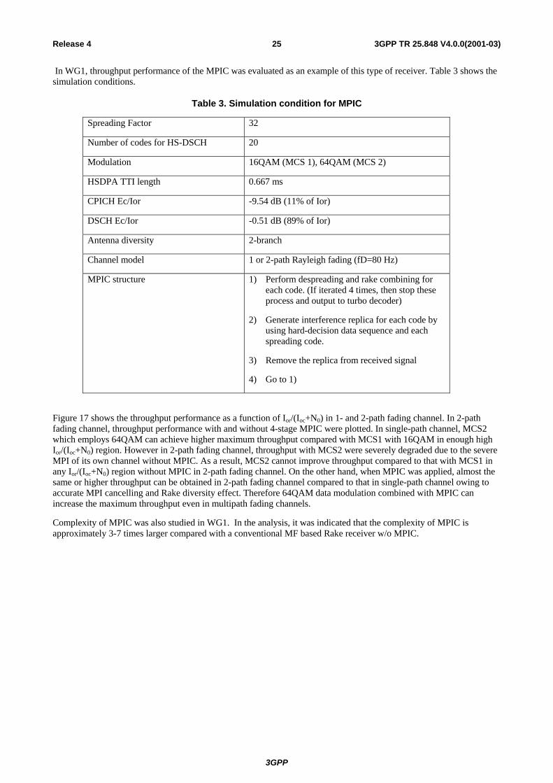
In WG1, throughput performance of the MPIC was evaluated as an example of this type of receiver. Table 3 shows the simulation conditions.

Table 3. Simulation condition for MPIC

Spreading Factor 32

Number of codes for HS-DSCH 20

Modulation 16QAM (MCS 1), 64QAM (MCS 2)

HSDPA TTI length 0.667 ms

CPICH Ec/Ior -9.54 dB (11% of Ior)

DSCH Ec/Ior -0.51 dB (89% of Ior)

Antenna diversity 2-branch

Channel model 1 or 2-path Rayleigh fading (fD=80 Hz)

MPIC structure 1) Perform despreading and rake combining for each code. (If iterated 4 times, then stop these process and output to turbo decoder)

2) Generate interference replica for each code by using hard-decision data sequence and each spreading code.

3) Remove the replica from received signal

4) Go to 1)

Figure 17 shows the throughput performance as a function of Ior/(Ioc+N0) in 1- and 2-path fading channel. In 2-path fading channel, throughput performance with and without 4-stage MPIC were plotted. In single-path channel, MCS2 which employs 64QAM can achieve higher maximum throughput compared with MCS1 with 16QAM in enough high Ior/(Ioc+N0) region. However in 2-path fading channel, throughput with MCS2 were severely degraded due to the severe MPI of its own channel without MPIC. As a result, MCS2 cannot improve throughput compared to that with MCS1 in any Ior/(Ioc+N0) region without MPIC in 2-path fading channel. On the other hand, when MPIC was applied, almost the same or higher throughput can be obtained in 2-path fading channel compared to that in single-path channel owing to accurate MPI cancelling and Rake diversity effect. Therefore 64QAM data modulation combined with MPIC can increase the maximum throughput even in multipath fading channels.

Complexity of MPIC was also studied in WG1. In the analysis, it was indicated that the complexity of MPIC is approximately 3-7 times larger compared with a conventional MF based Rake receiver w/o MPIC.

3GPP

3GPP TR 25.848 V4.0.0(2001-03)26Release 4

0 100

2 106

4 106

6 106

8 106

0 5 10 15 20 25

Thro

ughp

ut (b

its/s

ec)

Ior

/(Ioc

+N0) (dB)

1 path2 paths, w/o MPIC2 paths, with MPIC

MCS2MCS1

0 100

2 106

4 106

6 106

8 106

0 5 10 15 20 25

Thro

ughp

ut (b

its/s

ec)

Ior

/(Ioc

+N0) (dB)



MCS2MCS1

Figure 17. Throughput Performance of MPIC

6.7.5 Complexity Impacts to RNS The effect of higher order modulation on peak-to-average power ratio (PAP) at the Node-B transmitter was studied. Based on a very limited set of simulation experiments, it was observed that the PAP does not degrade compared to Release-99 downlink which only uses QPSK modulation. It was also noted PAP performance is very close to the analytic result. However, detailed analysis on the effect on PAP for a downlink using HS-DSCH needs to be carried out by WG#4.

6.8 Hybrid ARQ (H-ARQ)


6.8.1.1 Link Performance Comparison of Type-II and Type III HARQ Schemes

Chase Combining

The simplest form of Hybrid ARQ scheme was proposed by Chase [1]. The basic idea in Chase’s combining scheme (also called H-ARQ-type-III with one redundancy version) is to send a number of repeats of each coded data packet and allowing the decoder to combine multiple received copies of the coded packet weighted by the SNR prior to decoding. This method provides diversity gain and is very simple to implement.

H-ARQ with Partial IR (H-ARQ-Type-III)

Incremental redundancy is another H-ARQ technique wherein instead of sending simple repeats of the entire coded packet, additional redundant information is incrementally transmitted if the decoding fails on the first attempt. Incremental redundancy is called H-ARQ-type-II, or H-ARQ-type-III if each retransmission is restricted to be self-decodable. In this report both H-ARQ-type-II and H-ARQ-type-III was implemented for the MCS levels shown in Table 4.

3GPP

3GPP TR 25.848 V4.0.0(2001-03)27Release 4

Table 4. MCS Level for Method-2

MCS Modulation Turbo Code Rate 7 64 QAM 3/4 6 16 QAM 3/4 3 QPSK 3/4

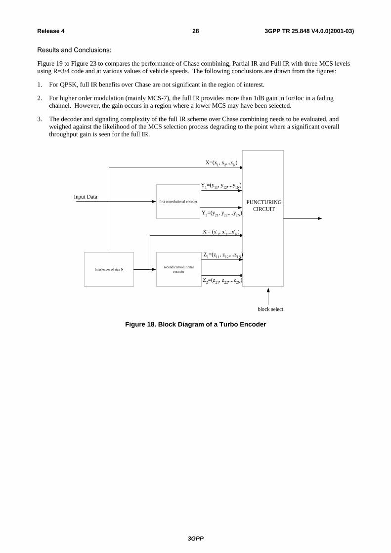
The turbo codes used in the hybrid ARQ system consists of a parallel concatenation of two R=1/3 systematic and recursive convolutional encoders as shown in Figure 18. The overall code rate of the turbo code entering the puncturing circuit is 1/6. For each input stream, six output streams are formed: the input stream x itself, two parity streams produced by the first convolutional code y1 and y2 interleaved input stream x’ and the second parity streams z2 and z3 produced by the second convolutional code. The puncturing block after the encoder is used to form (for example) R=3/4, R=2/3 and R=1/2 codes by puncturing the parity bits. As an example, for R=1/2 codes alternate parity bits are sent over the channel (x, y1, x, z2, x, y1,…). In case of partial IR using R=3/4 code the following algorithm was simulated:

• In case of even order transmission, the following set of coded bits are transmitted for every six information bits, : P1={xA, xB, xC, y1C, xD, xE, xF, z1F} In case of odd order transmission, the following set of systematic and parity bits are transmitted: P2={xA, xB, xC, y2C, xD, xE, xF, z2F} The very first transmission is decoded as an R=3/4 code, and subsequent re-transmissions are decoded as an R=3/5 code, where the bits in each subsequent retransmission are added symbol-wise to the corresponding stored bits.

The puncturing patterns P1 and P2 can be represented as the following two matrices. The multiplexing rule is to multiplex first by column, left to right. Within a column, read out top to bottom.

=

000000100000000000000000000100111111

1P

=

100000000000000000000100000000111111

2P

H-ARQ with Full IR (H-ARQ-Type-II)

In case of full IR using R=3/4 code the following algorithm was implemented:

• In case of first transmission, the following set of coded bits are transmitted for every six information bits, : P1={xA, xB, xC, y1C, xD, xE, xF, z1F} In case of second transmission (first re-transmission), the following set of parity bits are transmitted: P2={y1A, y2A, z1C, z2C, y2D, y1E, z1F, z2F} For the third transmission, a different set of parity bits are transmitted: P3={z1A, z2B, y1C, y2C, z2D, z1E, y1F, y2F}The sequence is then repeated.

• The very first transmission is decoded as an R=3/4 code, the next transmission is decoded as an R=3/8 code, and the third transmission is decoded as a R=1/4 code. Subsequent retransmissions are decoded as a R=1/4 code, where the bits in each subsequent retransmission are added symbol-wise to the corresponding stored bits.

The puncturing patterns P1, P2, and P3 can be represented as the following three matrices. The multiplexing rule is to multiplex first by column, left to right. Within a column, read out top to bottom.

=

000000100000000000000000000100111111

1P

=

100100100100000000001010010001000000

2P

=

001010010001000000100100100100000000

3P

3GPP

3GPP TR 25.848 V4.0.0(2001-03)28Release 4

Results and Conclusions:

Figure 19 to Figure 23 to compares the performance of Chase combining, Partial IR and Full IR with three MCS levels using R=3/4 code and at various values of vehicle speeds. The following conclusions are drawn from the figures:

1. For QPSK, full IR benefits over Chase are not significant in the region of interest.

2. For higher order modulation (mainly MCS-7), the full IR provides more than 1dB gain in Ior/Ioc in a fading channel. However, the gain occurs in a region where a lower MCS may have been selected.

3. The decoder and signaling complexity of the full IR scheme over Chase combining needs to be evaluated, and weighed against the likelihood of the MCS selection process degrading to the point where a significant overall throughput gain is seen for the full IR.

first convolutional encoder

Interleaver of size N second convolutionalencoder

X=(x1, x2,..xN)

Y1=(y11, y12,...y1N)

X'= (x'1, x'2,..x'N)

PUNCTURINGCIRCUIT

Input Data

block select

Y2=(y21, y22,...y2N)

Z1=(z11, z12,...z1N)

Z2=(z21, z22,...z2N)

Figure 18. Block Diagram of a Turbo Encoder

3GPP

3GPP TR 25.848 V4.0.0(2001-03)29Release 4

0Kmph Ec/Ior=-1dB

0.3

0.5

0.7

0.9

1.1

1.3

1.5

-14 -13 -12 -11 -10 -9 -8 -7

Ior/Ioc (dB)

Spec

tral

Eff.

QPSK R=3/4 Chase QPSK R=3/4 IR QPSK R=3/4 Full IR

Figure 19. Static QPSK

0Kmph Ec/Ior=-1dB

0.30.50.70.91.11.31.51.71.92.12.32.52.72.93.13.33.53.73.94.14.34.5

-8 -6 -4 -2 0 2

Ior/Ioc (dB)

Spec

tral

Eff.

16-QAM R=3/4 Chase 16-QAM R=3/4 IR 64-QAM R=3/4 Chase64-QAM R=3/4 IR 64-QAM R=3/4 Full IR 16-Qam R=3/4 Full IR

Figure 20. Static 16/64-QAM

3GPP

3GPP TR 25.848 V4.0.0(2001-03)30Release 4

3Kmph 2GHz 1-path Rayleigh Ec/Ior=-1dB

0.3

0.5

0.7

0.9

1.1

1.3

1.5

-11 -9 -7 -5 -3 -1 1 3 5 7 9

Ior/Ioc (dB)

Spec

tral

Eff.

QPSK R=3/4 Chase QPSK R=3/4 IR QPSK R=3/4 Full IR

Figure 21. 3 Kmph QPSK


0.30.50.70.91.11.31.51.71.92.12.32.52.72.93.13.33.53.73.94.14.34.5

-9 -7 -5 -3 -1 1 3 5 7 9 11 13

Ior/Ioc (dB)

Spec

tral

Eff.

16-QAM R=3/4 Chase 16-QAM R=3/4 IR 64-QAM R=3/4 Chase64-QAM R=3/4 IR 64-QAM R=3/4 Full IR 16-QAM R=3/4 Full IR

Figure 22. 3 Kmph 16/64-QAM

3GPP

3GPP TR 25.848 V4.0.0(2001-03)31Release 4


0.30.50.70.91.11.31.51.71.92.12.32.52.72.93.13.33.53.73.94.14.34.5

-9 -7 -5 -3 -1 1 3 5 7 9 11 13

Ior/Ioc (dB)

Spec

tral

Eff.

16-QAM R=3/4 Chase 16-QAM R=3/4 IR 64-QAM R=3/4 Chase64-QAM R=3/4 IR 64-QAM R=3/4 Full IR 16-QAM R=3/4 Full IR

Figure 23. 120 Kmph 16/64-QAM

6.8.2 Summary for CPICH SIR errors w/wo H-ARQ based on System Simulations:

The effect of CPICH SIR measurement errors (0,1 and 3dB) on throughput with and without Hybrid ARQ (chase combining) is studied using a dynamic system simulation tool. The system simulator tool models Rayleigh and Rician fading, time evolution with discrete steps (0.667ms e.g.), adaptive modulation and coding (AMC), fast Hybrid ARQ, fast cell selection FCS, and open loop transmit diversity (STTD). The simulator also models Lognormal shadowing, delay spread, and fractional recovered power (per ray). Most of the system simulation assumptions used are described in Annex().). The system simulation assumptions used are described in sections 12.3.2 to 12.3.7 and in Tdoc# R1-01-0046. Each UE experienced 3kph rayleigh fading with fractional recovered power of 0.98.

6.8.2.1 CPICH SIR Measurement Error model

In the adaptive modulation and coding (AMC) schemes proposed for HSDPA, the UE uses the CPICH to estimate the downlink SIR (also known as C/I or Ec/Nt) in the current slot. This information is then fed back on an uplink control channel. Node B then uses this estimate to determine the modulation and coding level for that users subsequent frame and possibly also for setting scheduling priorities. Past contributions by Motorola have assumed perfect estimation of the downlink SIR. The simulation results presented below give throughput statistics when the measured CPICH SIR is modeled as:

ˆCPICH CPICH CPICHSIR SIR= + ∆

where CPICHSIR and ˆCPICHSIR are the actual and estimated CPICH SIR respectively in dB and CPICH∆ is a Gaussian

random variable with standard deviation σ ∆ dB.

6.8.2.2 Hybrid ARQ (Chase combining) modeling

The system simulation tool models Chase combining process by accumulating the received signal energy of frame retransmissions. Based on this accumulated energy, a random number is drawn to determine if the frame is in error. In

3GPP

3GPP TR 25.848 V4.0.0(2001-03)32Release 4

equation form, the energy used to determine a frame error, ( )_ HARQError Energy k , is accumulated across k transmissions:

( ) ( )1

_k

HARQ DSCHi

Error Energy k E i=

= ∑

where ( )DSCHE k is the received energy of the kth frame.

Hybrid ARQ is disabled by simply neglecting the accumulated energy and basing frame error determination on the current frame energy:

( ) ( )__ NO HARQ DSCHError Energy k E k=

6.8.2.3 Simulation Results/Conclusions for CPICH SIR errors w/wo H-ARQ

Table 5 to Table 10 summarize best effort packet data throughput performance for a data only HSDPA system with a Maximum C/I scheduler and a modified ETSI source model. The different throughput metrics presented are defined in Annex C. The MCS used for the H-ARQ enabled case were QPSK R=1/2, 16QAM R=1/2, 16QAM R=3/4, and 64QAM R=3/4. The seven MCS used for the H-ARQ disabled case were QPSK R=1/4, QPSK R=1/2, QPSK R=3/4, 16QAM R=1/2, 8PSK R=1/2, 16QAM R=3/4, and 64QAM R=3/4. The minimum block size for the non-Hybrid ARQ case is set smaller (44 bytes versus 336 bytes) to allow more flexibility in allocating as small an MCS as needed for poor channels conditions which is important when H-ARQ is not available to help. This is needed to keep residual FER low.

From Table 5 to Table 7 we see that with H-ARQ on, there is a drop in packet call throughput of between 5% and 10% with 1 dB CPICH measurement error. Sector throughput decreases by only about 5%. For 3dB CPICH measurement error, however, the packet call throughput drop approaches 50% and the sector throughput drop reaches 20%. The columns marked "Residual FER" give the percentage of users whose frame error rate, after all retransmissions, is above 1% and .1%. Estimation errors of 1 dB are seen to cause only very small increases in residual error rate.

Comparing Table 5 to Table 7 with H-ARQ to Table 8 to Table 10 without H-ARQ we see a significant drop in packet call throughput and residual FER without H-ARQ as also illustrated in Figure 24 to Figure 26. (Note the throughputs are quite close for the no H-ARQ case when comparing 0dB and 1dB SIR measurement error cases. In some cases the throughputs are even slightly better for 1dB than 0dB. This is because the 10^-4 residual FER for the 1dB error case was not reduced enough to match the lower coresponding residual FER values achieved with 0dB error. If this was done then the throughputs for the 0dB error would have been consistantly better than the 1dB case)

In general every effort should be made to find algorithms which keep the CPICH SIR measurement error smaller than 3dB and preferably no larger than 1 dB.

Table 5. H-ARQ Enabled with CPICH Error σ=0dB Single Rayleigh Ray, 3kph, FRP=0.98 Blk Size=336 bytes Max C/I, Mod. ETSI 30% Overhead AMC, no FCS, HARQ, σ=0dB

User Packet Call %UEs with#Users per sector, Percent Offered Throughput CDF Residual FER

Max ovsf codes OTA Service Packet call Utilization Load <32k/64k/128k/384k/1M >10-2 / >10-4(bps) (bps) (bps) (%) (bps) (%) (%)

012ue/sect, 20size32 2,189,367 476,764 1,494,552 21.7 492,820 00 / 00 / 00 / 02 / 29 0.0 / 0.0037ue/sect, 20size32 1,934,215 1,422,217 1,164,068 72.0 1,475,268 00 / 00 / 02 / 16 / 49 0.0 / 1.0056ue/sect, 20size32 1,985,243 1,872,642 1,008,999 91.6 1,934,544 01 / 03 / 10 / 32 / 61 0.0 / 1.2075ue/sect, 20size32 2,251,443 2,312,162 943,371 99.2 2,371,219 05 / 09 / 21 / 43 / 65 0.3 / 2.0100ue/sect, 20size32 2,787,112 2,890,511 924,114 99.7 2,935,203 12 / 19 / 29 / 49 / 67 0.0 / 0.9

Average Throughput StatisticsCenter Cell




012ue/sect, 20size32 2,041,386 468,907 1,439,111 23.0 489,320 00 / 00 / 00 / 02 / 29 0.0 / 0.7037ue/sect, 20size32 1,769,061 1,359,925 1,091,056 74.8 1,396,482 00 / 00 / 02 / 18 / 53 0.0 / 2.0056ue/sect, 20size32 1,918,134 1,885,656 915,797 94.4 1,853,439 03 / 06 / 14 / 38 / 64 0.0 / 3.1075ue/sect, 20size32 2,106,633 2,186,367 841,139 99.0 2,188,733 05 / 11 / 23 / 46 / 69 0.3 / 2.4100ue/sect, 20size32 2,546,921 2,697,633 821,589 99.7 2,748,435 16 / 24 / 34 / 53 / 71 0.1 / 1.1

Center CellAverage Throughput Statistics

3GPP

3GPP TR 25.848 V4.0.0(2001-03)33Release 4




012ue/sect, 20size32 1,800,245 468,615 1,268,680 25.9 485,515 00 / 00 / 00 / 03 / 38 0.0 / 6.6037ue/sect, 20size32 1,539,392 1,327,651 857,181 81.6 1,367,491 00 / 01 / 05 / 28 / 65 0.1 / 21.6056ue/sect, 20size32 1,596,800 1,733,146 650,307 97.9 1,755,674 03 / 10 / 25 / 51 / 79 3.8 / 37.5075ue/sect, 20size32 1,739,118 2,010,782 548,694 99.7 2,028,803 17 / 28 / 41 / 62 / 84 10.8 / 45.1100ue/sect, 20size32 1,984,111 2,344,356 488,986 100.0 1,685,867 29 / 40 / 51 / 70 / 88 19.2 / 43.1


Table 8. H-ARQ Disabled with CPICH Error σ=0dB Single Rayleigh Ray, 3kph, FRP=0.98 Blk Size=44 bytes Max C/I, Mod. ETSI 30% Overhead AMC, no FCS, no HARQ, σ=0dB













012ue/sect, 20size32 651,769 421,017 562,266 64.7 428,874 02 / 12 / 22 / 50 / 85 0.0 / 27.3037ue/sect, 20size32 1,001,833 994,474 441,438 98.8 996,024 20 / 32 / 44 / 66 / 92 0.4 / 34.5056ue/sect, 20size32 1,289,235 1,299,310 404,842 99.9 1,318,800 32 / 42 / 53 / 73 / 93 1.8 / 33.2075ue/sect, 20size32 1,534,659 1,549,681 388,628 99.9 1,583,774 39 / 49 / 59 / 77 / 94 3.6 / 41.9100ue/sect, 20size32 1,856,090 1,887,593 379,859 100.0 1,932,895 46 / 56 / 64 / 80 / 95 6.2 / 33.7


3GPP

3GPP TR 25.848 V4.0.0(2001-03)34Release 4

0

10

20

30

40

50

60

70

80

0 200 400 600 800 1000 1200

(kbps)

Perc

Use

rs w

Pac

ket C

all T

hrou

ghpu

t < A

bsic

ca12ue/sector - no harq

37ue/sector - no harq




12ue/sector - harq

37ue/sector - harq

56ue/sector - harq

75ue/sector - harq

100ue/sector - harq

Figure 24. %User Packet Call Throughput CDF w/wo H-ARQ for the 1dB CPICH SIR measurement error case using a Max C/I Scheduler

0.0

5.0

10.0

15.0

20.0

25.0

30.0

35.0

12ue/sector 37ue/sector 56ue/sector 75ue/sector 100ue/sector

Perc

Use

rs w

Res

FER

> 1

0^-2

or 1

0^-4

10-2, Harq

10-2, noHarq

10-4, Harq

10-4, noHarq

Figure 25. Residual FER with and without H-ARQ for the 1dB CPICH SIR measurement error case using a Max C/I Scheduler

3GPP

3GPP TR 25.848 V4.0.0(2001-03)35Release 4

0

200,000

400,000

600,000

800,000

1,000,000

1,200,000

1,400,000

1,600,000

1,800,000

2,000,000

0 500,000 1,000,000 1,500,000 2,000,000 2,500,000 3,000,000

Service Throughput (bps)

Pack

et C

all T

hrou

ghpu

t (bp

s)0dB SIR Error (harq)1dB SIR Error (harq)3dB SIR Error (harq)0dB SIR Error (no harq)1dB SIR Error (no harq)3dB SIR Error (no harq)

Figure 26. Packet Throughput vs Service Throughput w/wo H-ARQ for different CPICH SIR Measurement Errors using a Max C/I Scheduler.

6.8.3 Complexity Evaluation <UE and RNS impacts>

6.8.3.1 N-channel stop-and-wait H-ARQ

6.8.3.1.1 Introduction

The complexity of H-ARQ mechanisms when employed for link adaptation in HSDPA transmission depends on the H-ARQ scheme selected as well as on where the retransmission functionality is located in the UTRAN. Dual-channel stop-and-wait (SAW) protocol has been proposed as the retransmission functionality for HDSPA. A complexity evaluation on SAW H-ARQ is presented in this section. In this complexity evaluation it is further assumed that H-ARQ retransmission protocol operates in Node B.

6.8.3.1.2 Buffering complexity

The principle of hybrid ARQ is to buffer HSDPA TTIs that were not received correctly and consequently combine the buffered data with retransmissions. The actual method of doing soft combining depends on the H-ARQ combining scheme selected. In Chase combining scheme the receiver always combines the full retransmission of the failed HSDPA TTI, i.e. the amount of data in the receiver buffer remains the same. In the incremental redundancy schemes the receiver buffers coded symbols, which introduce new information to the HSDPA TTI transmitted first, i.e. the amount of data to be buffered increases with consecutive retransmissions. However, probably in practice the buffer in the receiver needs to be dimensioned considering the maximum size of the HSDPA TTI after all the incremental redundancy has been introduced. Regardless of the H-ARQ combining scheme soft combining is done on L1 before the decoding stage of FEC. Prior to decoding these symbols are soft-valued, i.e. each symbol is represented by two or more bits.

Regardless of the location of retransmission functionality in the RNS the number of symbols to be buffered in L1 receiver can be estimated generally as follows:

( ))( NACKretransmitPDU latencylatencyTTIinPDUsfailedbitscodedbuffer +××=

where it is assumed for the sake of clarity that an integer number of PDUs fit into one HSDPA TTI. The latencies are also considered as multiples of a HSDPA TTI. For dual channel stop-and-wait H-ARQ the buffer size estimation is

3GPP

3GPP TR 25.848 V4.0.0(2001-03)36Release 4

considerably simplified since no new PDUs are transmitted on a subchannel before the previous packet is acknowledged. The receiver has to buffer one HSDPA TTI from both subchannels. The next transmission is either a new packet or a retransmission of an erroneous packet. In either case, the maximum buffering need is two HSDPA TTIs. The actual size of the buffer needed for each HSDPA TTI depends on the H-ARQ combining scheme as described above. The receiver buffering complexity estimate can be easily extended to n-channel stop-and-wait protocol, where at maximum n HSDPA TTIs would be buffered at any given time. Thus, for n-channel stop-and-wait ARQ the L1 buffering can be expressed as:

( )nbitscodedbuffer TTI ×=

However, it must be noted that the size of HSDPA TTI may change when the number of subchannels changes, i.e. TTI length for n-channel SAW HARQ can be shorter than one for dual channel SAW HARQ. Average receiver buffer sizes for dual channel HARQ for some bit rates are depicted in Figure 27.

Naturally, the number of subchannels in stop-and-wait ARQ is reflected in the amount of acknowledgment signaling needed to be sent to the transmitter. The complexity impact on RNS is mainly concentrated on Node B where the H-ARQ retransmission resides according to the current proposal. However, packet buffering is not as much an issue in Node B hardware.

0

5000

10000

15000

20000

25000

kbps

soft

sym

bols

dual channel 10 msdual channel 3.33 ms

dual channel 10 ms 672 2112 4032 23232dual channel 3.33 ms 224 704 1344 7744

8 32 64 384

Figure 27. Receiver L1 buffer size for dual channel SAW HARQ

As an example, Table 11 to Table 22 show maximum estimated receiver buffer sizes for 4-channel SAW HARQ. Chase combining, i.e. retransmission of a complete HSDPA TTI (one CRC per TTI, included in the bit rate) and SF = 16 or SF = 32 are assumed. In Tables 1-6 retransmitted TTIs are combined at modulation symbol level. It can be seen that the memory size does not increase with modulation since there are only two values to be buffered: I and Q.

Table 11 Buffer at soft combining stage for 1 code channel, HSDPA TTI = 3 slots

Maximum buffer size for N-channel SAW HARQ, N=4, 2.0 ms frame, modulation symbols (I,Q pairs) buffered (Ksymbols)

SF QPSK 8-PSK 16-QAM 64-QAM 16, 1 code channel or 32, 2 code channels

3.8 (max 480 kbps)

3.8 (max 720 kbps) 3.8 (max 960 kbps) 3.8 (max 1.44 Mbps)

Table 12 Buffer at soft combining stage for 10 code channels, HSDPA TTI = 3 slots


SF QPSK 8-PSK 16-QAM 64-QAM 16, 10 code channels or 32, 20 code channels

38.4 (max 4.8 Mbps)

38.4 (max 7.2 Mbps)

38.4 (max 9.6 Mbps)

38.4 (max 14.4 Mbps)

3GPP

3GPP TR 25.848 V4.0.0(2001-03)37Release 4

Table 13 Buffer at soft combining stage for 1 code channel, HSDPA TTI = 5 slots


SF

QPSK 8-PSK 16-QAM 64-QAM

16, 1 code channel or 32, 2 code channels

6.4 (max 480 kbps) 6.4 (max 720 kbps) 6.4 (max 960 kbps) 6.4 (max 1.44 Mbps)

Table 14. Buffer at soft combining stage for 10 code channels, HSDPA TTI = 5 slots


SF


16, 10 code channels or 32, 20 code channels

64 (max 4.8 Mbps) 64 (max 7.2 Mbps) 64 (max 9.6 Mbps) 64 (max 14.4 Mbps)

Table 15. Buffer at soft combining stage for 1 code channel, HSDPA TTI = 15 slots


SF


16, 1 code channel or 32, 2 code channels

19.2 (max 480 kbps)

19.2 (max 720 kbps) 19.2 (max 960 kbps) 19.2 (max 1.44 Mbps)

Table 16. Buffer at soft combining stage for 10 code channels, HSDPA TTI = 15 slots


SF


16, 10 code channels or 32, 20 code channels

192 (max 4.8 Mbps)

192 (max 7.2 Mbps) 192 (max 9.6 Mbps) 192 (max 14.4 Mbps)

Table 17 to Table 22 show the memory size at the input of the turbo decoder, i.e. demodulated baseband symbols. These values express the required memory should buffering be done on demodulated symbols. The memory size for QPSK is the same as for modulation symbol level combining (there is one symbol in I branch and one in Q branch). However, for higher modulation alphabets the memory size becomes clearly bigger. Note that these values are valid for Chase combining. For incremental redundancy HARQ more memory is required (if N different redundancy versions of similar size are transmitted the memory estimates have to be multiplied by N).

Table 17. Memory at the input of turbo decoder for 1 code channel, HSDPA TTI = 3 slots

Maximum buffer size for N-channel SAW HARQ, N=4, 2.0 ms frame, baseband symbols buffered (Ksymbols)



3GPP

3GPP TR 25.848 V4.0.0(2001-03)38Release 4

Table 18. Memory at the input of turbo decoder for 10 code channels, HSDPA TTI = 3 slots


SF QPSK 8-PSK 16-QAM 64-QAM 16, 10 code channels or 32, 20 code channels

38.4 ( max 4.8 Mbps)

57.6 (max 7.2 Mbps)

76.8 (max 9.6 Mbps)

115 (max 14.4 Mbps)








64 (max 4.8 Mbps) 96 (max 7.2 Mbps) 128 (max 9.6 Mbps) 192 (max 14.4 Mbps)








192 (max 4.8 Mbps)

288 (max 7.2 Mbps) 384 (max 9.6 Mbps) 576 (max 14.4 Mbps)

6.8.3.1.3 Encoding/decoding and rate matching complexity

In order to facilitate incremental redundancy it is likely that the FEC encoder rate has to be lowered, i.e. instead of a 1/3 rate encoder, a 1/5 or even lower rate encoder would be employed. For example, as proposed this far, by puncturing different symbols out of the output code word, different redundancy information is generated for soft combining. A mother code of lower rate does increase the complexity of both encoding and decoding stage. However, it is not necessary to add new constituent encoders to a turbo coder in order to lower the coding rate. More advanced methods that output more than one symbol per bit per branch could be utilized. Furthermore, investigations are needed to check whether the existing rate matching algorithm of Rel –99 can be used in conjunction with incremental redundancy or whether modification of either the rate matching or the encoder are necessary"

6.8.3.1.4 UE and RNS processing time considerations

Stop-and-wait HARQ introduces several tasks for UE and RNS to process in order to have the uplink and downlink transmissions consistent.

3GPP

3GPP TR 25.848 V4.0.0(2001-03)39Release 4

Node B processing tasks prior to sending data in the HS-DSCH

• Decode the ACK/NACK transmitted in uplink

• Make a scheduling decision on which UE is due to receive data among the UEs having data in the transmission buffer

• Set TFCI and other information fields on downlink control channels

UE processing tasks

• Decode TFCI, HSDPA TTI sequence info etc.

• Despreading and demodulation

• Soft combine retransmitted HSDPA TTI in the receiver buffer for the correct subchannel

• Decode HSDPA TTI for the subchannel

• Check CRC to decide whether the HSDPA TTI was received correctly

• Generate ACK/NACK signaling for uplink

The time required for processing the tasks depends on the number of timeslots in the HSDPA TTI (number of bits to be processed). On the other hand, the time available for finishing the tasks also depends on these same factors. Figure 28 and Figure 29 show the general sequence of UE and RNS processing with two and four HARQ subchannels, respectively. In the figures Tprop depicts the propagation time, TUEP the processing time in UE, TACK the duration of ACK/NACK message, and TNBP the processing time in Node B.

Figure 28. Timing relations for 2-channel HARQ process

HSPDSCH at Node B

HSDPA TTI

UL feedback at UE

UL feedback at Node B

HSPDSCH at UE

UE channel 1

ACK/NACK

UE channel 1

ACK/NACK

UE channel 2 UE channel 2 UE channel 1


TUEP

TNBP

Tprop

Tprop

TACK

3GPP

3GPP TR 25.848 V4.0.0(2001-03)40Release 4

Figure 29. Timing relations for 4-channel HARQ process

The total time Tprocess available for UE and RNS processing can be expressed as:

The processing time can be roughly evaluated as in Table 23. The effect of propagation time can be considered negligible and it is not shown in the figures. It is assumed that TACK duration is one slot.

Table 23. Approximate time for UE and RNS processing with SAW HARQ

2 subchannels 4 subchannels Parameter 1-slot TTI 3-slot TTI 5-slot TTI 15-slot TTI 1-slot TTI 3-slot TTI 5-slot TTI 15-slot TTI Tprocess 0 ms 1.33 ms 2.67 ms 9.33 ms 1.33 ms 5.33 ms 9.33 ms 29.33 ms

The shorter the HSDPA TTI the less time there is available for processing. On the other hand, shorter TTI length reduces the time required for turbo decoding stage. The reduced processing time from shorter TTI length can be offset by increasing the number of subchannels. The actual amount of time required for processing is naturally implementation dependent. By making a rough assumption that both the UE and Node B use the same period of time, an estimate for the processing time can be made by dividing the figures in Table 21 by two.

In practice, there is some control/signal information transmitted by the Node B related to the data sent on HSPDSCH. Among other things this message could inform the UE of whether there is something sent to it during the particular HSDPA TTI, e,g, whether to read a control channel. This control/signal information could be transmitted at the same time as the respective TTI on HSPDSCH, which requires buffering the TTI at the UE. On the other hand, if this kind of information is sent prior to the respective HSDPA TTI, it is easier for the UE to know from which Node B the transmission is coming from and buffering TTIs possibly from several Node Bs is not needed. Sending the control/signal information early, however, reduces the Node B processing time TNBP. This effect is depicted in Figure 30 where TCTRL is the time needed for sending control/signal information.

propACKNBPUEP TTTTINTT ⋅−−⋅−=+ 2)1(

HSPDSCH at UE

HSDPA TTI


UL feedback at UE

UE channel 1

ACK/NACK

UE channel 1

ACK/NACK


UE channel 1 UE channel 1

TUEP

TNBP

Tprop

Tprop

TACK

HSPDSCH at Node B

HSPDSCH at UE

HSDPA TTI


UL feedback at UE

UE channel 1

ACK/NACK

UE channel 1

ACK/NACK


UE channel 1 UE channel 1

TUEP

TNBP

Tprop

Tprop

TACK

HSPDSCH at Node B

TCTRL

3GPP

3GPP TR 25.848 V4.0.0(2001-03)41Release 4

Figure 30. Timing relations for 4-channel HARQ process with downlink control/signal information prior to HSPDSCH transmission

6.8.3.1.5 Conclusions

Based on the complexity considerations presented above SAW HARQ is a feasible concept for HSDPA system, and it can be implemented. There is a difference in complexity between different HARQ schemes, e.g. Chase combining vs. IR, but these differences do not justify that any scheme is discarded at this stage. However, care must be taken with regard to processing time. The effect of HSDPA TTI length and the number of HARQ subchannels directly impact the available processing time in UE and RNS.

6.9 Fast Cell Selection (FCS)


6.9.1.1 Summary for FCS benefit:

The effect of Fast Cell Selection (FCS) on throughput is studied using a dynamic system simulation tool for data only system. The system simulator tool models Rayleigh and Rician fading, time evolution with discrete steps (0.667ms e.g.), adaptive modulation and coding (AMC), fast Hybrid ARQ, fast cell selection FCS, and open loop transmit diversity (STTD). The simulator also models Lognormal shadowing, delay spread, and fractional recovered power (per ray). The system simulation assumptions used are described in sections 12.3.2 to 12.3.7 and in Tdoc# R1-01-0047. Each UE experienced 3kph rayleigh fading with fractional recovered power of 0.98. It may be noted that time for transfer between Node-B’s are not included in the simulation results.

6.9.1.2 Conclusion for FCS benefit:

Fast Cell Selection (FCS) improves throughput and residual FER for UEs in multi-coverage regions (see Table 24 to Table 27 and Figure 32 through Figure 34). This is because a UE in a multi-coverage region typically has a weaker channel to any single serving cell compared to UEs closer to their serving cell. With FCS the multi-coverage UE has more opportunities to select a better link to one of the serving cells and be scheduled. The overall system benefit due to FCS is more significant with fair (in term of scheduling oppurtunities) schedulers (such as Round Robin) compared to maximum C/I scheduler since the users with weak links are scheduled more often. With a maximum C/I scheduler the larger the load the less impact FCS has on performance. Without FCS it takes longer for UEs with weak links to finish a packet call and hence longer to release the dedicated control channel which results in further overhead and reduced system capacity. Similar conclusions, i.e.FCS is primarily beneficial for Round-robin type scheduling and for users at the cell border, were drawn in Tdoc# R1-01-0036. Open issues include how much larger the FCS benefit is with motion and allowing for MCS changes between re-transmissions.

6.9.1.3 FCS function description

Fast Cell Selection (FCS) allows a UE to rapidly choose any one cell in its active set (i.e. set of potential serving cells) for down link transmission. The potential benefit is that for each frame interval the active set cell with the best faded link can be chosen for frame transmission to the UE. The UE chooses the best cell by comparing each active set cell’s estimated CPICH Ec/Io and transmits a cell indicator to be detected by the desired cell on a uplink dedicated control channel. Frame retransmissions can therefore take place by any active set cell if chosen and the resulting received signal energy from each frame is accumulated to model a Chase combining process. Note that the active set evolves with time as a UEs position changes. In this simulation the UEs experience fast (Rayleigh) fading but did not move from the initial location for a given Monte Carlo drop.

As part of the adaptive modulation and coding (AMC) schemes proposed for HSDPA, the UE also estimates CPICH Ec/Nt (C/I) for each cell in its pilot active set for the current slot. The pilot Ec/Nt information for the selected cell is then also fed back on an uplink dedicated control channel. The Node B then uses the C/I estimate to determine the modulation and coding level for that users subsequent frame and possibly also for setting scheduling priorities. The simulation results presented below compare throughput and residual FER statistics with and without FCS enabled. The cell selection update rate is once every 3.33ms. The FCS and CPICH measurement delay, as shown in Figure 31 below, is about 10ms.

3GPP

3GPP TR 25.848 V4.0.0(2001-03)42Release 4

MeasureCPICH

ReportC/ICell Indicator

SchedulePick MCS

Transmit

F.I.F.I. = 3.33ms

Figure 31. Time diagram of FCS and CPICH measurement delay

Table 24. FCS Disabled with Max C/I Scheduler Single Rayleigh Ray, 3kph, FRP=0.98 Block Size=336 bytes Max C/I, Mod. ETSI 30% Overhead AMC, HARQ, no FCS



012ue/sect, 20size32 2,338,440 387,204 1,568,007 16.5 399,220 00/00/00/01/23 0.0 / 0.2037ue/sect, 20size32 2,035,561 1,140,388 1,277,785 55.2 1,172,408 00/00/01/11/43 0.0 / 0.4056ue/sect, 20size32 2,120,471 1,679,382 1,131,307 77.4 1,720,800 00/01/05/23/53 0.0 / 0.4075ue/sect, 20size32 2,391,955 2,155,493 1,057,189 87.5 2,201,708 02/05/12/32/58 0.0 / 0.5100ue/sect, 20size32 2,798,980 2,670,794 1,011,444 91.9 2,716,026 07/13/21/40/62 0.0 / 0.4

Entire SystemAverage Throughput Statistics

Table 25. FCS Enabled with Max C/I Scheduler Single Rayleigh Ray, 3kph, FRP=0.98 Block Size=336 bytes Max C/I, Mod. ETSI 30% Overhead AMC, HARQ, FCS



012ue/sect, 20size32 2,420,614 393,447 1,588,520 16.2 405,329 00/00/00/00/21 0.0 / 0.0037ue/sect, 20size32 1,997,291 1,148,252 1,274,242 56.4 1,181,163 00/00/00/08/43 0.0 / 0.0056ue/sect, 20size32 2,049,253 1,699,108 1,109,216 80.7 1,742,468 00/01/04/22/53 0.0 / 0.0075ue/sect, 20size32 2,345,164 2,171,345 1,041,938 89.6 2,213,770 02/05/12/32/58 0.0 / 0.0100ue/sect, 20size32 2,766,521 2,692,171 996,139 93.5 2,739,260 07/13/21/40/63 0.0 / 0.0

Average Throughput StatisticsEntire System

From Table 26 and Table 27 for the Round Robin scheduler see somewhat larger throughput improvements with FCS on compared to the Maximum C/I scheduler. Figure 32 (based on center cell only results) illustrates FCS benefits by showing the %User Packet Cell throughput CDF with and without FCS at different loading. Figure 33 shows the increase in the average number of dedicated channels required to support the users that are not in the dormant state (waiting for all the packets of a packet call). Figure 34 and Figure 35 compare throughput performance and fairness for Round Robin and Maximum C/I schedulers.

Table 26. FCS Disabled with Round Robin Scheduler Single Rayleigh Ray, 3kph, FRP=0.98 Block Size=336 bytes RRobin, Mod. ETSI 30% Overhead AMC, HARQ, no FCS



012ue/sect, 20size32 2,157,079 389,284 1,507,379 17.9 401,654 00 / 00 / 00 / 01 / 23 0.0 / 0.1037ue/sect, 20size32 1,497,979 1,111,120 904,903 72.8 1,136,996 00 / 00 / 02 / 21 / 64 0.0 / 0.6056ue/sect, 20size32 1,328,442 1,470,168 446,527 100.0 1,476,561 02 / 11 / 30 / 65 / 91 0.0 / 1.6075ue/sect, 20size32 1,308,320 1,630,910 254,732 100.0 1,598,901 17 / 40 / 60 / 88 / 96 0.0 / 1.3


Table 27. FCS Enabled with Round Robin Scheduler Single Rayleigh Ray, 3kph, FRP=0.98 Block Size=336 bytes RRobin, Mod. ETSI 30% Overhead AMC, HARQ, FCS



012ue/sect, 20size32 2,282,522 391,198 1,547,580 17.0 397,347 00 / 00 / 00 / 00 / 19 0.0 / 0.0037ue/sect, 20size32 1,548,366 1,133,420 957,866 71.8 1,161,699 00 / 00 / 00 / 13 / 60 0.0 / 0.1056ue/sect, 20size32 1,326,962 1,524,255 426,340 100.0 1,532,878 00 / 05 / 26 / 64 / 93 0.0 / 0.2075ue/sect, 20size32 1,299,941 1,690,414 230,325 100.0 1,665,984 11 / 36 / 58 / 89 / 97 0.0 / 0.2


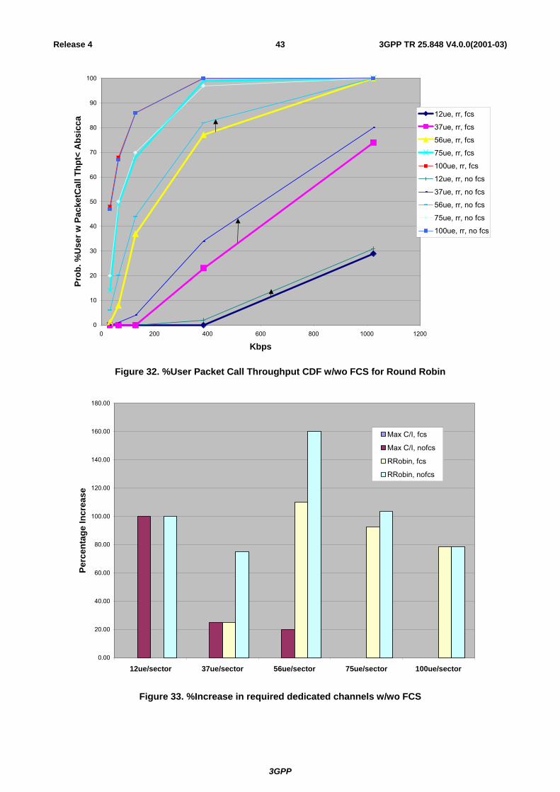
3GPP

3GPP TR 25.848 V4.0.0(2001-03)43Release 4

0

10

20

30

40

50

60

70

80

90

100

0 200 400 600 800 1000 1200

Kbps

Prob

. %U

ser w

Pac

ketC

all T

hpt<

Abs

icca

12ue, rr, fcs

37ue, rr, fcs

56ue, rr, fcs

75ue, rr, fcs

100ue, rr, fcs

12ue, rr, no fcs

37ue, rr, no fcs

56ue, rr, no fcs

75ue, rr, no fcs

100ue, rr, no fcs

Figure 32. %User Packet Call Throughput CDF w/wo FCS for Round Robin

0.00

20.00

40.00

60.00

80.00

100.00

120.00

140.00

160.00

180.00

12ue/sector 37ue/sector 56ue/sector 75ue/sector 100ue/sector

Perc

enta

ge In

crea

se

Max C/I, fcs

Max C/I, nofcs

RRobin, fcs

RRobin, nofcs

Figure 33. %Increase in required dedicated channels w/wo FCS

3GPP

3GPP TR 25.848 V4.0.0(2001-03)44Release 4

0

200,000

400,000

600,000

800,000

1,000,000

1,200,000

1,400,000

1,600,000

1,800,000

2,000,000

0 500,000 1,000,000 1,500,000 2,000,000 2,500,000 3,000,000

Service Throughput (bps)

Pack

et T

hrou

ghpu

t (bp

s)

mci, fcs on

mci, fcs off

rr, fcs on

rr, fcs off

All Users Still Scheduled (100ue/sector)

Figure 34. Packet Throughput vs Service Throughput for Max C/I and Round Robin

0

10

20

30

40

50

60

70

80

90

100

0 200 400 600 800 1000 1200

Kbps

Prob

. %U

ser w

Pac

ketC

all T

hpt<

Abs

icca

12ue, rr, fcs

56ue, rr, fcs

75ue, rr, fcs

100ue, rr, fcs

12ue, mci, fcs

56ue, mci, fcs

75ue, mci, fcs

100ue, mci, fcs

Max C/I

Round Robin

Figure 35. Fairness: %User Packet Call Throughput CDF comparing Maximum C/I with Round Robin Schedulers at 3kph.

3GPP

3GPP TR 25.848 V4.0.0(2001-03)45Release 4

6.9.2 Complexity Evaluation <UE and RNS impacts> As discussed in conclusions of Section 6.4, FCS could inherit a significant part of the required physical-layer functionality from SSDT. Thus FCS will not have a major impact on the UE complexity. The impact on RNS complexity remains to be studied.

6.10 Multiple input multiple output antenna processing

6.10.1 MIMO performance evaluation Link level simulations were performed and the frame error rate (FER) versus Ior/Ioc were measured for a variety of system architectures. We first compare the systems for a fixed data rate and show that, compared to the conventional transmitter, MIMO architectures can achieve the same frame error rate at much lower Ior/Ioc. Next, we show how for a similar Ior/Ioc, the MIMO architectures can achieve higher data rates. Using the notation (M,P) to denote a system with M transmit and P receive antennas, we study a conventional (1,1) system, a (2,2) MIMO system, and a (4,4) MIMO system.

The data rate was fixed at 10.8 Mbps, achieved assuming a chipping rate of 3.84 Mchips/sec, a spreading factor of 32 chips per coded symbol, N = 20 spreading codes, and appropriate coding rates and data constellation sizes. A parallel concatenated convolutional coding and turbo decoding with 8 decoding iterations was used. The system architectures for M transmit antennas and P receive antennas are given in Table 28.

Puncturing for the (4,4) system is used to achieve 10.8 Mbps. A flat fading channel with 3km/hr fading, perfect channel estimation, and uncorrelated fading between antenna pairs for the MIMO systems is assumed. Figure 36 below shows the FER versus Ior/Ioc. Compared to the conventional transmitter, there are gains of about 9dB and 16dB for the (2,2) and (4,4) systems, respectively, at 10% FER. The enormous performance gains are due to a combination of diversity, receiver combining gain, and increased spectral efficiency due to MIMO processing. We emphasize that these gains are achieved using the same code resources (20 codes) as the conventional transmitter.

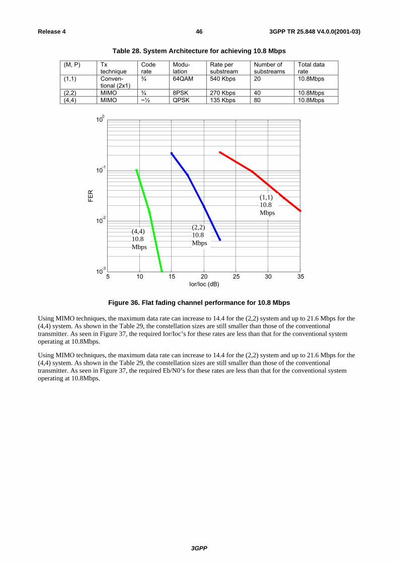
3GPP

3GPP TR 25.848 V4.0.0(2001-03)46Release 4

Table 28. System Architecture for achieving 10.8 Mbps

(M, P) Tx technique

Code rate

Modu-lation

Rate per substream

Number of substreams

Total data rate

(1,1) Conven-tional (2x1)

¾ 64QAM 540 Kbps 20 10.8Mbps

(2,2) MIMO ¾ 8PSK 270 Kbps 40 10.8Mbps (4,4) MIMO ~½ QPSK 135 Kbps 80 10.8Mbps

5 10 15 20 25 30 3510

-3

10-2

10-1

100

Ior/Ioc (dB)

FER

(4,4)10.8Mbps

(2,2)10.8Mbps

(1,1)10.8Mbps

Figure 36. Flat fading channel performance for 10.8 Mbps

Using MIMO techniques, the maximum data rate can increase to 14.4 for the (2,2) system and up to 21.6 Mbps for the (4,4) system. As shown in the Table 29, the constellation sizes are still smaller than those of the conventional transmitter. As seen in Figure 37, the required Ior/Ioc’s for these rates are less than that for the conventional system operating at 10.8Mbps.

Using MIMO techniques, the maximum data rate can increase to 14.4 for the (2,2) system and up to 21.6 Mbps for the (4,4) system. As shown in the Table 29, the constellation sizes are still smaller than those of the conventional transmitter. As seen in Figure 37, the required Eb/N0’s for these rates are less than that for the conventional system operating at 10.8Mbps.

3GPP

3GPP TR 25.848 V4.0.0(2001-03)47Release 4

Table 29. System Architecture for achieving 21.8 Mbps

(M, P) Tx technique

Code rate

Modu-lation

Rate per substream

Number of substreams

Total data rate

(1,1) Conven-tional (2x1)

¾ 64QAM 540 Kbps 20 10.8Mbps

(2,2) MIMO ¾ 16QAM 360 Kbps 40 14.4Mbps (4,4) MIMO ¾ QPSK 180 Kbps 80 14.4Mbps (4,4) MIMO ¾ 8PSK 540 Kbps 80 21.6Mbps

5 10 15 20 25 30 3510

-3

10-2

10-1

100

Ior/Ioc (dB)

FER

(4,4)14.4Mbps

(4,4)21.6Mbps

(2,2)14.4Mbps

(1,1)10.8Mbps

Figure 37. Flat fading channel performance for higher data rates

One way to interpret the Ior/Ioc gains for MIMO is that the high data rates can be achieved with less transmit power. Alternatively, if the DSCH is transmitted at a fixed power, then the MIMO gains translate into the higher data rates being used over a larger fraction of the cell area. Under this assumption of a rate-controlled DSCH, a system level study employing a base station scheduler showed that the average sector throughput using a (4,4) MIMO system increases by a factor of 1.8 and 2.8 for proportional fair and maximum C/I scheduling, respectively, compared to a conventional (1,1) system (As an aside, a surprising result is that under a proportional fair scheduler, the conventional (1,1) system actually outperforms both the (2,1) and (4,1) diversity systems when there are multiple users vying for the DSCH.). It may be noted that the system level simulation did not use all the assumptions as outlined in Annex A.

Additional link level studies presented to RAN WG1 investigated the effect of higher doppler frequencies and channel estimation. These studies indicate that a worst case loss in required Ior/Ioc of only about 2dB. In non-ideal channel conditions, there may be spatial channel correlations which could potentially degrade MIMO performance. Given a parametric model for modeling spatial correlations in multiple antenna channels based on antenna separations and anglular spreads at both the UE and Node B, parameters can be chosen to model a microcellular environment. Link level results shown below indicate insignificant performance degradation for the (2,2) system. The (4,4) systems are less robust, but losses can be mitigated by transmitting with two of the four antennas and using larger constellations. In fact, as shown by the figure below, performance gains can be achieved by transmitting from the worst two antennas (worst in the sense of highest correlation). The resulting performance is within 2dB of the ideal uncorrelated (4,4) performance. For comparison, spatial correlations modeled by actual MIMO channel measurements have also been derived. Preliminary results presented to RAN WG1 indicate similar performance trends derived from the theoretical model given above.

3GPP

3GPP TR 25.848 V4.0.0(2001-03)48Release 4

5 10 15 20 25 30 3510

-3

10-2

10-1

100

Ior/Ioc (dB)

FER

(1,1) conventional(2,2) uncorrelated channels,ML(2,2) correlated channels, ML

Figure 38. FER for (2,2) system, 10.8 Mbps, flat channel, 3km/hr

5 10 15 20 25 30 3510-3

10-2

10-1

100

Ior/Ioc (dB)

FER

(1,1) conventional(4,4) uncorrelated channels, ML

(2,4) uncorrelated channels, ML(4,4) correlated channels, VBLAST(2,4) correlated channels,worst 2 of 4 transmitters, ML

(4,4) uncorrelated channels, VBLAST

Figure 39. FER for 4 receive antenna system, 10.8 Mbps, flat channel, 3km/hr

3GPP

3GPP TR 25.848 V4.0.0(2001-03)49Release 4

6.10.2 MIMO UE complexity evaluation The MIMO UE will require multiple uncorrelated antennas and additional baseband processing to perform space-time combining and spatial processing on substreams which share the same code.

High spectral efficiencies of the MIMO system are achieved when there is uncorrelated fading among pairs of transmitter and receiver antennas. With 2GHz carrier frequency, an array of 4 antennas with dual-polarization requires only 7.5cm of linear space. Because the terminal receiver is at the same level as local scatterers, ½ wavelength antenna spacing can generally achieve a fair amount of decorrelation of multipath signals, particularly in cases in which there is no direct path between receiver and transmitter (Rayleigh fading) [1] . However, the final correlation could be increased by factors such as the proximity to the human body and other objects

A complexity estimate for MIMO receivers was presented to RAN WG1 which includes an outline complexity breakdown for specific UE components including antenna components, RF signal processing, baseband signal processing, fixed costs, and processing for layers 2 and above. It indicates that – compared to a single antenna receiver operating at 10.8Mbps – the complexity of a 4 antenna MIMO receiver operating at 21.6 Mbps would be up to 2 times greater.

However, performance data for the receiver that formed the basis for this complexity analysis has only been offered for time non-dispersive channels, and additional baseband signal processing (including chip-level processing such as equalization or interference cancellation) may be required to deal with delay-spread conditions. Further, a common model for UE complexity evaluation has not yet been established in TSG-RAN WG1 and the UE complexity estimate presented to RAN WG1 has not been verified by other manufacturers. Accordingly, while the presented complexity estimates are useful, they should be regarded as very preliminary.

6.10.3 Node-B Complexity Evaluation The block diagram for M antenna MIMO HSDPA transmission is shown in Figure 6 in Section 6.5. A single antenna transmitter demultiplexes the high speed data stream into N lower rate substreams (N is the number of Walsh spreading codes) whereas the MIMO transmitter demultiplexes the stream into MN lower rate substreams. In terms of baseband processing, the MIMO demultiplexers require minimal additional complexity over the single antenna demultiplexers. For backwards compatibility, non-MIMO transmission on other dedicated channels are transmitted over antenna 1. The MIMO and non-MIMO signals will not interfere with each other since the Walsh codes used are mutually orthogonal. Orthogonal pilot sequences are also transmitted from each antenna to allow for timing acquisition, synchronization, and/or channel estimation.

The power of the MIMO transmissions are normalized so that for the DSCH so the total transmit power summed across the M antennas is the same as for the single antenna transmission. Hence while multiple power amplifiers are required for MIMO transmission, (typically one per transmit antenna), the loading on any of these amplifiers will be reduced compared to the power amplifier in a single antenna system. Furthermore, because MIMO transmission uses smaller data constellations, the peak-to-average power ratio could also be reduced.

In the same way that transmit diversity techniques rely on uncorrelated fading among pairs of transmitter and receiver antennas, high spectral efficiencies of the MIMO system also rely on uncorrelated fading. The correlation depends on the spacing between antennas and height of the antennas with respect to the local scatterers. For outdoor base stations where the antennas are significantly higher than the scatterers, totally uncorrelated fading is achieved using a separation of 10 wavelengths between nearest neighbors in a linear base array of dual-polarized antennas. For indoor base stations, or in situations where the antennas are at the same height as the local scatterers, the scatterers will cause more decoupling of the signals at the antennas. Hence, the required antenna separation for a given level of correlation will be even less.

7 Physical layer aspects for TDD mode This section describes the techniques behind the concept of HSDPA for the TDD mode.

7.1 Techniques to support HSDPA for TDD mode In the previous chapters technologies were presented to improve the air interface utilisation. The principles of the described technologies are applicable for both, FDD and TDD, however the methods and details have only been

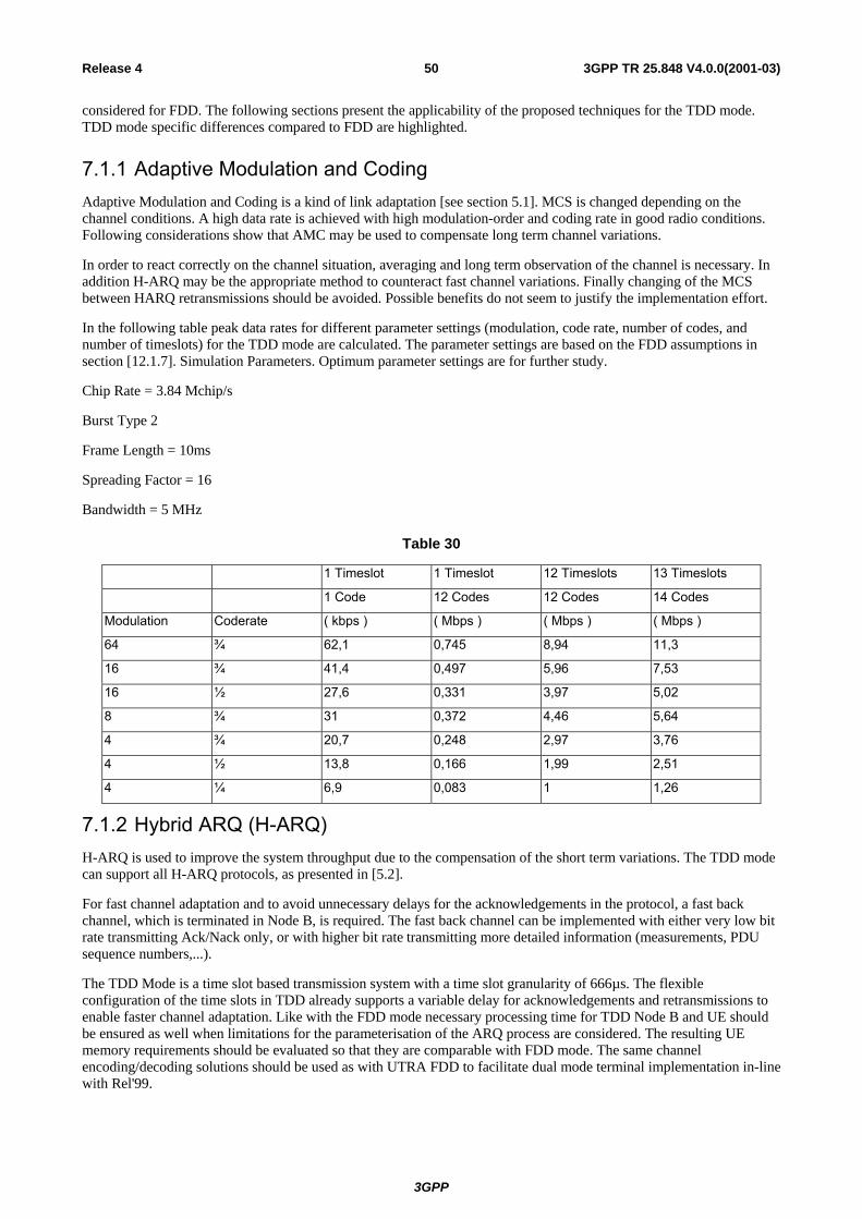
3GPP

3GPP TR 25.848 V4.0.0(2001-03)50Release 4

considered for FDD. The following sections present the applicability of the proposed techniques for the TDD mode. TDD mode specific differences compared to FDD are highlighted.

7.1.1 Adaptive Modulation and Coding Adaptive Modulation and Coding is a kind of link adaptation [see section 5.1]. MCS is changed depending on the channel conditions. A high data rate is achieved with high modulation-order and coding rate in good radio conditions. Following considerations show that AMC may be used to compensate long term channel variations.

In order to react correctly on the channel situation, averaging and long term observation of the channel is necessary. In addition H-ARQ may be the appropriate method to counteract fast channel variations. Finally changing of the MCS between HARQ retransmissions should be avoided. Possible benefits do not seem to justify the implementation effort.

In the following table peak data rates for different parameter settings (modulation, code rate, number of codes, and number of timeslots) for the TDD mode are calculated. The parameter settings are based on the FDD assumptions in section [12.1.7]. Simulation Parameters. Optimum parameter settings are for further study.

Chip Rate = 3.84 Mchip/s

Burst Type 2

Frame Length = 10ms

Spreading Factor = 16

Bandwidth = 5 MHz

Table 30

1 Timeslot 1 Timeslot 12 Timeslots 13 Timeslots

1 Code 12 Codes 12 Codes 14 Codes

Modulation Coderate ( kbps ) ( Mbps ) ( Mbps ) ( Mbps )

64 ¾ 62,1 0,745 8,94 11,3

16 ¾ 41,4 0,497 5,96 7,53

16 ½ 27,6 0,331 3,97 5,02

8 ¾ 31 0,372 4,46 5,64

4 ¾ 20,7 0,248 2,97 3,76

4 ½ 13,8 0,166 1,99 2,51

4 ¼ 6,9 0,083 1 1,26

7.1.2 Hybrid ARQ (H-ARQ) H-ARQ is used to improve the system throughput due to the compensation of the short term variations. The TDD mode can support all H-ARQ protocols, as presented in [5.2].

For fast channel adaptation and to avoid unnecessary delays for the acknowledgements in the protocol, a fast back channel, which is terminated in Node B, is required. The fast back channel can be implemented with either very low bit rate transmitting Ack/Nack only, or with higher bit rate transmitting more detailed information (measurements, PDU sequence numbers,...).

The TDD Mode is a time slot based transmission system with a time slot granularity of 666µs. The flexible configuration of the time slots in TDD already supports a variable delay for acknowledgements and retransmissions to enable faster channel adaptation. Like with the FDD mode necessary processing time for TDD Node B and UE should be ensured as well when limitations for the parameterisation of the ARQ process are considered. The resulting UE memory requirements should be evaluated so that they are comparable with FDD mode. The same channel encoding/decoding solutions should be used as with UTRA FDD to facilitate dual mode terminal implementation in-line with Rel'99.

3GPP

3GPP TR 25.848 V4.0.0(2001-03)51Release 4

7.1.3 Fast Cell Selection (FCS) FCS has been proposed with the FDD mode for HS-DSCH to be used in case of soft handover is applied with the associated DCH. With TDD mode FCS is not directly applicable, since with the TDD mode in Rel'99 UEs can send and receive from a single Node B only. Additionally UTRAN needs to control in TDD mode the transmission in time domain in terms of which slot(s) accommodate the UE transmission. Thus FCS implementation effort does not seem to reflect possible benefits.

7.1.4 MIMO The use of Multiple Input Multiple Output (MIMO) techniques haven been proposed for FDD mode. As such these techniques are applicable for UTRA TDD as well, but there are issues that require TDD specific considerations for UTRA TDD. Especially the impact on the TDD UE receiver should be carefully considered.

7.2 Simulation assumptions Table 31 presents the link level simulation assumptions for TDD. They are aligned with those for FDD (Annex A), whenever this is possible. However, some TDD specific parameters have to be taken into account.

Table 31. Link Level Simulation Assumption

Parameter Value CommentsCarrier Frequency 2GHzPropagation conditions AWGN, Indoor AVehicle Speed for Flat Fading 3 kmhClosed loop Power Control OFFHSDPA frame Length 10msIor/Ioc VariableChannel Estimation Real (on the midamble) / Ideal As definedFast fading model Jakes spectrum

Channel codingTurbo Decoder and Rate Matching asSpecified in Release-99 Specification see AMCS Table, see [2]

Tail bits 6 per RSC encoderMax no. of iterations for Turbo Coder 4Input to Turbo Decoder SoftHybrid ARQ As definedInformation Bit Rates (Kbps) As defined see AMCS TableNumber of Multicodes Simulated As defined see AMCS Table

TFCI model

Random symbols, ignored in the receiverbut it is assumed that the receiver getserror free reception of TFCI information

Reciever Joint Detection (ZF-BLE)Oversampling NoChiprate 3.84 McpsFramestructure 15 TS per 10ms see AMCS TableSF 16Burst type 2Modulation Scheme As defined see AMCS TableOther L1 Parameters As Specified in Release-99 Specification

7.3 Link-level simulation results This chapter presents link level simulation results using the link-level simulation assumptions of chapter 8.2 for the AMC schemes given in 8.1. Results are shown for the case, where 13 timeslots and 14 codes are allocated for the HS-DSCH. No HARQ is employed and a real channel estimation on the midamble is used.

Figure 40 depicts the FER vs. Eb/No of the seven MCS for the AWGN channel. Figure 41 shows the corresponding results for the Indoor A channel.

3GPP

3GPP TR 25.848 V4.0.0(2001-03)52Release 4

1,00E-03

1,00E-02

1,00E-01

1,00E+00

1 2 3 4 5 6 7 8 9 10 11 12 13

Eb/No [dB]

FER

MCS1 MCS2 MCS3 MCS4 MCS5 MCS6 MCS7

Figure 40. FER, AWGN Channel

1,00E-03

1,00E-02

1,00E-01

1,00E+00

6 8 10 12 14 16 18 20 22 24 26 28

Eb/No [dB]

FER

MCS1 MCS2 MCS3 MCS4 MCS5 MCS6 MCS7

Figure 41. FER, Indoor A channel

The above simulations show that higher order modulation is applicable for the TDD mode. The presented link level performance results are comparable with those for FDD given in chapter 12. However, a direct numerical comparison is not possible due to some differences in the simulation assumptions. The TDD simulations are using real channel estimation on the midamble in contrast to the FDD simulations, which are based on ideal channel estimation. Furthermore the Indoor A model was selected instead of the simple one ray model.

As a result of the performance similarities between TDD and FDD an alignment of the AMC schemes for both modes seems to be possible.

3GPP

3GPP TR 25.848 V4.0.0(2001-03)53Release 4

8 Backwards compatibility aspects (void)

9 Conclusions and recommendations 1. Adaptive Modulation and Coding (AMC):

Based on numerous discussion and simulation results, it was observed that a HS-DSCH with AMC and Hybrid ARQ can provide substantial higher peak rates and average throughput than the current Release-99 DSCH. As such, RAN1 concluded that AMC should be part of Release 5 HS-DSCH.

2. Fast Cell Selection:

RAN1 recommends that the study of intra-Node B and inter-Node B Fast Cell Selection should be considered together and not separately. Although, initial simulation studies indicate that some benefit with FCS can be observed in some cases the results are not conclusive. In view of the above RAN1 recommends that both intra and inter Node-B FCS should be studied further during Release#5 HSDPA work so that it can be a part of Release-6 specification.

3. MIMO:

The goal of HS-DSCH is to increase the average throughput as well as the peak data rate. MIMO represents a promising approach but there are a wide variety of applicable MIMO techniques which should be investigated along with MIMO examples in the TR during the standardisation process. It may also be noted that, the performance advantage of MIMO schemes is heavily dependent on the underlying channel model. The channel model should be agreed upon in RAN1 and will be used to verify different techniques. In view of the above, RAN1 recommends that MIMO should be part of further HSDPA work.

4. Stand-alone DSCH:

RAN 1 identified that the stand-alone DSCH was a specific case of mapping of transport channels for a UE in a multi-carrier cell. If a work item on multi-carrier cells was to be considered at RAN, RAN 1 recommends that a study item parallel to HSDPA is introduced to study the benefits of stand-alone DSCH for HSDPA as part of the UTRAN evolution.

3GPP

3GPP TR 25.848 V4.0.0(2001-03)54Release 4

Annex A: Simulation Assumptions and Results

A.1 Link simulation assumptions

A.1.1 Link assumptions The objective of this section is to propose a set of definitions, assumptions, and a general framework for performing initial link level simulations for High Speed Downlink Packet Access (HSDPA). The objective of these link level simulations is to provide the needed input data to initial system level simulations and to evaluate the link performance of different Adaptive Modulation and Coding schemes and fast Hybrid ARQ methods.

A.1.2 Simulation description overview A symbol level downlink simulator may be used to simulate the performance of higher order modulation schemes and Hybrid ARQ. The general forward link simulation model is shown in Figure 1. The terminology used throughout the document is as follows: Ior is the total transmitted power density by a BTS, orI is the post-channel transmitted power

density, ooc NI + is the other cell interference plus noise power density and Io is the total received power density at the MS antenna. Note, that the ratio

( )oocor NII +/ˆ is fixed in this simulation model. Since the base station has a fixed amount of power (set by the BTS power amplifier size), it is the average transmitted (often called allocated) power by the BTS to the MS that determines the user capacity of the forward link. This fraction of allocated power is called average traffic channel Ec/Ior and is inversely proportional to the forward link capacity.

Base Station(Transmitter)

Channelh(t)

Interference from OtherCells + Thermal Noise

Mobile Station(Receiver)

Ior

Ec/Ior

Ior Io

Ioc+ No

FER/BER

Figure 42. Simulation Block Diagram.

A.1.3 Standard constellations for m-ary modulation In case of 8-PSK modulation, every three binary symbols from the channel interleaver output shall be mapped to a 8-PSK modulation symbol according to Figure 2.

3GPP

3GPP TR 25.848 V4.0.0(2001-03)55Release 4

0.9239

0.9239

0.3827

0.3827

-0.9239

-0.9239 -0.3827

-0.3827

I-Channel

Q-Channel

000

100

001011

010

110

111 101

Figure 43. Signal Constellation for 8-PSK Modulation.

In case of 16-QAM modulation, every four binary symbols of the block interleaver output shall be mapped to a 16-QAM modulation symbol according to Figure 3.

1011 1001 0001 0011

1010 1000 0000 0010

1110 1100 0100 0110

1111 1101 0101 0111

i2 i2

i1

q1

q2

q2

0.3162 0.94870.31

620.

9487

Figure 44. Signal Constellation for 16-QAM Modulation.

In case of 64-QAM modulation, every six binary symbols of the block interleaver output shall be mapped to a 64-QAM modulation symbol according to Figure 4.

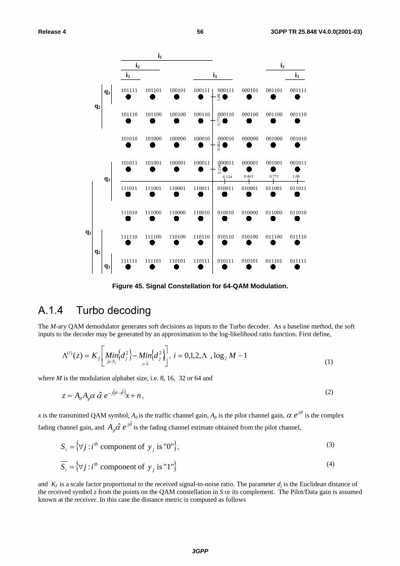
3GPP

3GPP TR 25.848 V4.0.0(2001-03)56Release 4

i1

101111 101101 100101 100111 000111 000101 001101 001111

101110 101100 100100 100110 000110 000100 001100 001110

101010 101000 100000 100010 000010 000000 001000 001010

101011 101001 100001 100011 000011 000001 001001 001011

i3 i3 i3

i2 i2

q1

q2

q3

q3

q3

q2

0.154 0.463 0.771 1.08

0.15

40.

463

0.77

11.

08

111011 111001 110001 110011 010011 010001 011001 011011

111010 111000 110000 110010 010010 010000 011000 011010

111110 111100 110100 110110 010110 010100 011100 011110

111111 111101 110101 110111 010111 010101 011101 011111

Figure 45. Signal Constellation for 64-QAM Modulation.

A.1.4 Turbo decoding The M-ary QAM demodulator generates soft decisions as inputs to the Turbo decoder. As a baseline method, the soft inputs to the decoder may be generated by an approximation to the log-likelihood ratio function. First define,

{ } { }

−=Λ

∈∈

22)( )( jjSjfi dMindMinKz

Siji

, 1log,,2,1,0 2 −= Mi Λ

(1)

where M is the modulation alphabet size, i.e. 8, 16, 32 or 64 and

( ) nxeAAz jpd += −− θθαα ˆˆ , (2)

x is the transmitted QAM symbol, Ad is the traffic channel gain, Ap is the pilot channel gain, θα je is the complex

fading channel gain, and θα ˆ ˆ jp eA is the fading channel estimate obtained from the pilot channel,

{ }"0" is ofcomponent : jth

i yijS ∀= , (3)

{ }"1" is ofcomponent : jth

i yijS ∀= (4)

and Kf is a scale factor proportional to the received signal-to-noise ratio. The parameter dj is the Euclidean distance of the received symbol z from the points on the QAM constellation in S or its complement. The Pilot/Data gain is assumed known at the receiver. In this case the distance metric is computed as follows

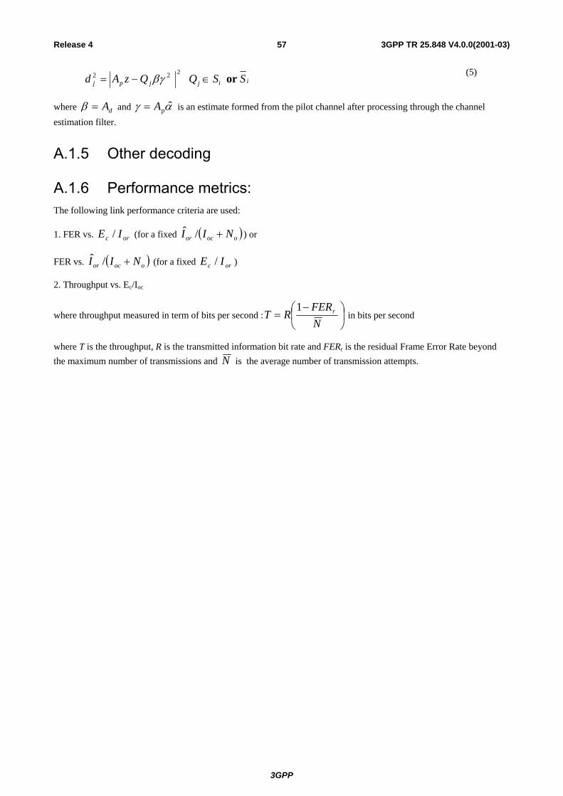
3GPP

3GPP TR 25.848 V4.0.0(2001-03)57Release 4

222 βγjpj QzAd −= iij SSQ or ∈ (5)

where dA=β and αγ ˆpA= is an estimate formed from the pilot channel after processing through the channel estimation filter.

A.1.5 Other decoding

A.1.6 Performance metrics: The following link performance criteria are used:

1. FER vs. orc IE / (for a fixed ( )oocor NII +/ˆ ) or

FER vs. ( )oocor NII +/ˆ (for a fixed orc IE / )

2. Throughput vs. Ec/Ioc

where throughput measured in term of bits per second :

−=

NFER

RT r1 in bits per second

where T is the throughput, R is the transmitted information bit rate and FERr is the residual Frame Error Rate beyond the maximum number of transmissions and N is the average number of transmission attempts.

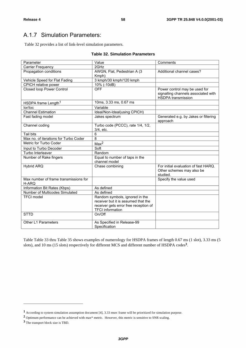
3GPP

3GPP TR 25.848 V4.0.0(2001-03)58Release 4

A.1.7 Simulation Parameters: Table 32 provides a list of link-level simulation parameters.

Table 32. Simulation Parameters

Parameter Value Comments Carrier Frequency 2GHz Propagation conditions AWGN, Flat, Pedestrian A (3

Kmph) Additional channel cases?

Vehicle Speed for Flat Fading 3 kmph/30 kmph/120 kmph CPICH relative power 10% (-10dB) Closed loop Power Control OFF Power control may be used for

signalling channels associated with HSDPA transmission

HSDPA frame Length1 10ms, 3.33 ms, 0.67 ms Ior/Ioc Variable Channel Estimation Ideal/Non-Ideal(using CPICH) Fast fading model Jakes spectrum Generated e.g. by Jakes or filtering

approach Channel coding Turbo code (PCCC), rate 1/4, 1/2,

3/4, etc.

Tail bits 6 Max no. of iterations for Turbo Coder 8 Metric for Turbo Coder Max2 Input to Turbo Decoder Soft Turbo Interleaver Random Number of Rake fingers Equal to number of taps in the

channel model

Hybrid ARQ Chase combining For initial evaluation of fast HARQ. Other schemes may also be studied.

Max number of frame transmissions for H-ARQ

Specify the value used

Information Bit Rates (Kbps) As defined Number of Multicodes Simulated As defined TFCI model Random symbols, ignored in the

receiver but it is assumed that the receiver gets error free reception of TFCI information

STTD On/Off

Other L1 Parameters As Specified in Release-99 Specification

Table Table 33 thru Table 35 shows examples of numerology for HSDPA frames of length 0.67 ms (1 slot), 3.33 ms (5 slots), and 10 ms (15 slots) respectively for different MCS and different number of HSDPA codes3.

1 According to system simulation assumption document [4], 3.33 msec frame will be prioritized for simulation purpose. 2 Optimum performance can be achieved with max* metric. However, this metric is sensitive to SNR scaling. 3 The transport block size is TBD.

3GPP

3GPP TR 25.848 V4.0.0(2001-03)59Release 4

Table 33. Information bit rate for frame duration of 0.67 msec

Chip Rate = 3.84 Mcps SF = 32 Frame Size = 0.67 ms

MCS 20 codes 1 code Code rate Modulation

Info Rate Info bits/frame Info Rate Info bits/frame (Mbps) (bits) (octets) (Mbps) (bits) (octets)

7 10.8000 7200 900 0.54 360 45 3/4 64

6 7.2000 4800 600 0.36 240 30 3/4 16 5 4.8000 3200 400 0.24 160 20 1/2 16 4 5.4000 3600 450 0.27 180 22.5 3/4 8 3 3.6000 2400 300 0.18 120 15 3/4 4 2 2.4000 1600 200 0.12 80 10 1/2 4 1 1.2000 800 100 0.06 40 5 1/4 4

Table 34 . Information bit rate for frame duration of 3.33 msec




7 10.8000 36000 4500 0.54 1800 225 3/4 64

6 7.2000 24000 3000 0.36 1200 150 3/4 16 5 4.8000 16000 2000 0.24 800 100 1/2 16 4 5.4000 18000 2250 0.27 900 112.5 3/4 8 3 3.6000 12000 1500 0.18 600 75 3/4 4 2 2.4000 8000 1000 0.12 400 50 1/2 4 1 1.2000 4000 500 0.06 200 25 1/4 4

Table 35. Information bit rate for frame duration of 10 msec




7 10.8000 1E+05 13500 0.54 5400 675 3/4 64

6 7.2000 72000 9000 0.36 3600 450 3/4 16 5 4.8000 48000 6000 0.24 2400 300 1/2 16 4 5.4000 54000 6750 0.27 2700 337.5 3/4 8 3 3.6000 36000 4500 0.18 1800 225 3/4 4 2 2.4000 24000 3000 0.12 1200 150 1/2 4 1 1.2000 12000 1500 0.06 600 75 1/4 4

3GPP

3GPP TR 25.848 V4.0.0(2001-03)60Release 4

A.1.8 Simulation cases

A.2 Link simulation results For the HSDPA study item, an AMC scheme using 7 MCS levels as outlined in Table-4 of the Annex were simulated using a symbol level link simulator. The AMC scheme uses QPSK, 8-PSK and 16 and 64 QAM modulation using R=1/2 and R=3/4 Turbo code and can support a maximum peak data rate of 10.8 Mbps.

Figure 47 to Figure 49 shows some sample FER vs. Ior/Ioc curves for various MCS levels for a fixed power allocation of –1dB. It may be observed that as the order of MCS is increased the Ior/Ioc requirements gets higher to achieve the same FER.

Figure 50 to Figure 52 shows the throughput performance of the AMC at 3 kmph and with Hybrid ARQ (Chase combining) enabled/disabled. Figure 53 to Figure 55 shows the performance of the AMC at 120 kmph and with Hybrid ARQ (Chase combining) enabled/disabled. The following abbreviations are used in the Figures:

CE – Channel Estimation – 0(ideal), 1 (non-ideal)

STTD – Transmit Diversity – 0(off), 1(on)

NC – Number of codes

ARQ – Hybrid ARQ using Chase combining – 0(off), 1(on)

NP – Number of paths

FC – Carrier frequency (2 GHz)

IBM – Ray Imbalance

ECIOR = Power Allocation (set to 80%)

SPEED – Vehicle speed

Q – QAM Modulation Level (4/8/16/64)

CR – Turbo Code Rate

MR – Maximum number of repeats

The following observations are made from the figures:

a. MCS level 1 (R=1/4 using QPSK) and MCS level 3 (R=3/4 using 8 PSK) does not have any throughput advantages for geometries (Ior/Ioc) ranging from 0 dB to 20dB. In view of the above, the number of MCS levels can easily be reduced from 7 to 5.

b. The power requirement doubles as the number of codes are doubled.

c. AMC with HARQ provides higher throughput than AMC without Hybrid ARQ especially at slow speeds. A HARQ system with fast feedback, can ensure that extra redundancy is sent only when needed while still meeting delay constraints.

3GPP

3GPP TR 25.848 V4.0.0(2001-03)61Release 4

ff=0 ce=0 sttd=0 arq=0 np=1 fe=2000 ibm=0 ecior=-1

1.00E-03

1.00E-02

1.00E-01

1.00E+00

-20 -15 -10 -5 0 5 10

Ior/Ioc

FER

q=64 cr=0.75 nc=1 mr=1 mph=0 q=64 cr=0.75 nc=2 mr=1 mph=0 q=16 cr=0.75 nc=1 mr=1 mph=0 q=16 cr=0.75 nc=2 mr=1 mph=0q=16 cr=0.5 nc=1 mr=1 mph=0 q=16 cr=0.5 nc=2 mr=1 mph=0 q=8 cr=0.75 nc=1 mr=1 mph=0 q=8 cr=0.75 nc=2 mr=1 mph=0q=4 cr=0.75 nc=1 mr=1 mph=0 q=4 cr=0.75 nc=2 mr=1 mph=0 q=4 cr=0.5 nc=1 mr=1 mph=0 q=4 cr=0.5 nc=2 mr=1 mph=0q=4 cr=0.25 nc=1 mr=1 mph=0 q=4 cr=0.25 nc=2 mr=1 mph=0 Series1

Figure 46. FER vs. Ior/Ioc for various MCS schemes Channel -Static

ff=0 ce=0 sttd=1 arq=0 np=1 fe=2000 ibm=0 ecior=-1 mph=1.86

1.00E-05

1.00E-04

1.00E-03

1.00E-02

1.00E-01

1.00E+00

-20 -15 -10 -5 0 5 10

Ior/Ioc

FER

q=4 cr=0.75 nc=1 mr=1 q=4 cr=0.75 nc=2 mr=1 q=4 cr=0.5 nc=1 mr=1 q=4 cr=0.5 nc=2 mr=1 q=4 cr=0.25 nc=1 mr=1 q=4 cr=0.25 nc=2 mr=1

Figure 47. FER vs. Ior/Ioc for QPSK – Flat Fading @3 kmph

3GPP

3GPP TR 25.848 V4.0.0(2001-03)62Release 4


1.00E-03

1.00E-02

1.00E-01

1.00E+00

-6 -4 -2 0 2 4 6 8 10 12 14

Ior/Ioc

FER

q=16 cr=0.75 nc=1 mr=1 q=16 cr=0.75 nc=2 mr=1 q=16 cr=0.5 nc=1 mr=1 q=16 cr=0.5 nc=2 mr=1

Figure 48. FER vs. Ior/Ioc for 16 QAM– Flat Fading @ 3Kmph


1.00E-03

1.00E-02

1.00E-01

1.00E+00

0 5 10 15 20 25

Ior/Ioc

FER

q=64 cr=0.75 nc=1 mr=1 q=64 cr=0.75 nc=2 mr=1

Figure 49. FER vs. Ior/Ioc for 64-QAM – Flat Fading @ 3Kmph

3GPP

3GPP TR 25.848 V4.0.0(2001-03)63Release 4

ff=0 ce=0 sttd=1 nc=1 arq=1 np=1 fe=2000 ibm=0 ecior=-1 mph=1.86

0

2

4

6

8

10

12

-5 0 5 10 15 20

Ior/Ioc

Thro

ughp

ut

q=64 cr=0.75 mr=10 q=16 cr=0.75 mr=10 q=16 cr=0.5 mr=10 q=8 cr=0.75 mr=10 q=4 cr=0.75 mr=10 q=4 cr=0.5 mr=10 q=4 cr=0.25 mr=10 Hull of sttd=1 arq=1

Figure 50. Throughput at 3kmph with HARQ


0

2

4

6

8

10

12

-5 0 5 10 15 20

Ior/Ioc

Thro

ughp

ut


Figure 51. Throughput at 3 kmph without HARQ

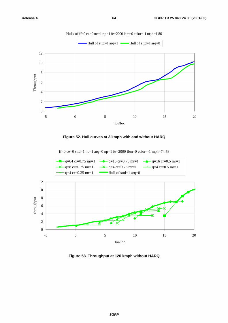
3GPP

3GPP TR 25.848 V4.0.0(2001-03)64Release 4

Hulls of ff=0 ce=0 nc=1 np=1 fe=2000 ibm=0 ecior=-1 mph=1.86

0

2

4

6

8

10

12

-5 0 5 10 15 20

Ior/Ioc

Thro

ughp

ut

Hull of sttd=1 arq=1 Hull of sttd=1 arq=0

Figure 52. Hull curves at 3 kmph with and without HARQ


0

2

4

6

8

10

12

-5 0 5 10 15 20

Ior/Ioc

Thro

ughp

ut



3GPP

3GPP TR 25.848 V4.0.0(2001-03)65Release 4


0

2

4

6

8

10

12

-5 0 5 10 15 20

Ior/Ioc

Thro

ughp

ut



Hulls of ff=0 ce=0 nc=1 np=1 fe=2000 ibm=0 ecior=-1 mph=74.58

0

2

4

6

8

10

12

-5 0 5 10 15 20

Ior/Ioc

Thro

ughp

ut

Hull of sttd=1 arq=1 Hull of sttd=1 arq=0

Figure 55. Hull curves at 120 kmph with and without HARQ

A.2.1 Effect of multipath

A.2.2 Effect of non-ideal channel estimation: Figure 56 and Figure 57 show the FER versus Ior/Ioc for QPSK modulation in a 1-path Rayleigh with vehicle speed of 3kmph and 120kmph respectively. Figure 58 and Figure 59 show the FER versus Ior/Ioc for 16QAM modulation in a 1-path Rayleigh with vehicle speed of 3kmph and 120kmph respectively. Notice that with ideal channel estimation (ICE),

3GPP

3GPP TR 25.848 V4.0.0(2001-03)66Release 4

the FER performance at higher vehicle speed is better than that at lower vehicle speed for both QPSK and 16QAM due to more un-correlated errors at higher speed. However, for the higher speed case, the channel estimation errors are generally large due to the time-variant behaviour of the channel. Such channel estimation errors may dramatically degrade the performance as shown in the figures. For higher modulation, such as 16QAM and 64QAM, the channel estimation accuracy is more important because of the close signal constellation and both phase and magnitude related soft input calculation.

Figure 56. FER versus Ior/Ioc , R=1/2 QPSK, 3 kmph

Figure 57 FER versus Ior/Ioc , R=1/2 QPSK, 120 kmph

3GPP

3GPP TR 25.848 V4.0.0(2001-03)67Release 4

Figure 58 FER versus Ior/Ioc , R=1/2 16 QAM, 120 kmph.

Figure 59 FER versus Ior/Ioc , R=1/2 QAM, 120 kmph.

Conclusion

Preliminary simulation results regarding the effect of channel estimation error on the link level performance of HSDPA is shown. The link level performance of higher order modulation is very sensitive to the channel estimation (used for channel compensation and other purposes) and thus accurate channel estimation is essential, especially at high vehicle speeds. More investigation on this topic and novel techniques to handle this practical issue are needed.

A.3 System simulation assumptions The scope of this section is to propose a set of definitions and assumptions on which HSDPA simulations can be based. The initial objective of such system simulations should be to illustrate/verify the potential performance gains due to the currently proposed HSDPA features, such as adaptive modulation and coding scheme (AMCS), fast Hybrid ARQ, and fast cell selection (FCS).

3GPP

3GPP TR 25.848 V4.0.0(2001-03)68Release 4

A.3.1 Common system level simulation assumptions As system level simulation tools and platforms differ between companies very detailed specification of common simulation assumptions is not feasible. Yet, basic simulation assumptions and parameters should be harmonized as proposed in the subsequent chapters. Various kinds of system performance evaluation methods may be used. In Annex 1, two different methods are outlined. They should be seen as examples and therefore other methods can be used.

A.3.2 Basic system level parameters The basic system level simulation parameters are listed in Table 5 below.

Table 36. Basic system level simulation assumptions.

Parameter Explanation/Assumption Comments Cellular layout Hexagonal grid, 3-sector sites Provide your cell layout picture Site to Site distance 2800 m Antenna pattern As proposed in [2] Only horizontal pattern specified Propagation model L = 128.1 + 37.6 Log10(R) R in kilometers CPICH power -10 dB Other common channels - 10 dB Power allocated to HSDPA transmission, including associated signaling

Max. 80 % of total cell power

Slow fading As modeled in UMTS 30.03, B 1.4.1.4 Std. deviation of slow fading 8 dB Correlation between sectors 1.0 Correlation between sites 0.5 Correlation distance of slow fading

50 m

Carrier frequency 2000 MHz BS antenna gain 14 dB UE antenna gain 0 dBi UE noise figure 9 dB Max. # of retransmissions Specify the value used Retransmissions by fast HARQ

Fast HARQ scheme Chase combining For initial evaluation of fast

HARQ BS total Tx power Up to 44 dBm Active set size 3 Maximum size Specify Fast Fading model Jakes spectrum Generated e.g. by Jakes or

Filter approach

A.3.3 Data traffic model The described data-traffic model simulates bursty web traffic. The parameters of the model are based on [4] but have been tailored to reduce simulation run time by decreasing the number of UEs required to achieve peak system loading. The main modification is to reduce the reading time between packet calls. In addition, TCP/IP rate adaptation mechanisms have been included to pace the packet arrival process of packets within a packet call.

The model assumes that all UEs dropped are in an active packet session. These packet sessions consist of multiple packet calls representing Web downloads or other similar activities. Each packet call size is modeled by a truncated Pareto distributed random variable producing a mean packet call size of 25 Kbytes. Each packet call is separated by a reading time. The reading time is modeled by a Geometrically distributed random variable with a mean of 5 seconds. The reading time begins when the UE has received the entire packet call.

Each packet call is segmented into individual packets. The time interval between two consecutive packets can be modeled in two ways, as an open loop process or as a closed loop process. The open loop process models the timer interval as a geometrically distributed random variable. Specifically, the mean packet inter-arrival time will be set to the ratio of the maximum packet size divided by the peak link speed. The closed loop model will incorporate the “slow-start” TCP/IP rate control mechanism for pacing packet traffic. Slow-start will be implemented as described in [5]. A total round trip network delay of 100 ms will be assumed for TCP ACK feedback.

3GPP

3GPP TR 25.848 V4.0.0(2001-03)69Release 4

The fundamentals of the data-traffic model are captured in Table 6.

Table 37. Data-traffic model parameters.

Process Random Variable Parameters Packet Calls Size Pareto with cutoff Α=1.1, k=4.5 Kbytes, m=2 Mbytes, µ =

25 Kbytes Time Between Packet Calls Geometric µ = 5 seconds Packet Size Segmented based on MTU size (e.g. 1500 octets) Packets per Packet Call Deterministic Based on Packet Call Size and Packet

MTU Packet Inter-arrival Time (open- loop)

Geometric µ = MTU size /peak link speed (e.g. [1500 octets * 8] /2 Mbps = 6 ms)

Packet Inter-arrival Time (closed-loop)

Deterministic TCP/IP Slow Start (Fixed Network Delay of 100 ms)

A.3.4 UE mobility model A static or dynamic UE mobility model can be used. Both fixed UE speed or a speed distribution may be used. In the latter case the speed distribution given in Figure 5 shall be used, see also Table 7. A speed is assigned to each user at the beginning of the simulation and will not be changed during the simulation. Stationary UEs signal paths will be Rician faded with K factor of 12dB and 2Hz Doppler spread.

Pedestrian & Low Mobility Speed Distribution

0

5

10

15

20

25

30

35

40

0 20 40 60 80 100 120

Speed (kph)

Perc

enta

ge C

alls

Speed PDF

Figure 60. Pedestrian and low mobility speed distribution.

Table 38. Speed distribution

Speed (kph) 0 1 3 8 10 15 20 30 40 50 60 70 80 90 100Percentage 14 37 15 1 1 2 6 10 7 2 1 1 1 1 1

A.3.5 Packet scheduler Multiple types of packet schedulers may be simulated. However, initial results may be provided for the two simple schedulers provided below that bound performance. The first scheduler (C/I based) provides maximum system capacity at the expense of fairness, because all frames can be allocated to a single user with good channel conditions. The Round Robin (RR) scheduler provides a more fair sharing of resources (frames) at the expense of a lower system capacity.

Both scheduling methods obey the following rules:

An ideal scheduling interval is assumed and scheduling is performed on a frame by frame basis.

3GPP

3GPP TR 25.848 V4.0.0(2001-03)70Release 4

The “frame” is defined by the HSDPA concept, e.g. 0.67ms (1 slot), 3.33ms (5 slots), or 10 ms (15 slots).

A queue is 'non-empty' if it contains at least 1 octet of information.

Packets received in error are explicitly rescheduled after the ARQ feedback delay consistent with the HSDPA definition.

A high priority queue is maintained to expedite the retransmission of failed packet transmission attempts. Entry into the high priority queue will be delayed by a specified time interval (e.g. 5 frame intervals) to allow for scheduler flexibility4. If the packet in the high-priority queue is not rescheduled after a second time interval (e.g. 10 frame intervals) it is dropped.

Packets from the low priority queue may only be transmitted after the high-priority queue is empty.

Transmission during a frame cannot be aborted or pre-empted for any reason

The C/I scheduler obeys the following additional rules:

At the scheduling instant, all non-empty source queues are rank ordered by C/I for transmission during a frame.

The scheduler may continue to transfer data to the UE with the highest C/I until the queue of that UE is empty, data arrives for another UE with higher C/I, or a retransmission is scheduled taking higher priority.

Both high and low priority queues are ranked by C/I.

The RR scheduler obeys the following rules:

At the scheduling instant, non-empty source queues are serviced in a round-robin fashion.

All non-empty source queues must be serviced before re-servicing a user.

Therefore, the next frame cannot service the same user as the current frame unless there is only one non-empty source queue.

The scheduler is allowed to group packets from the selected source queue within the frame.

A.3.6 Outputs and performance metrics The following suggested performance metrics for both the entire system and the center site taken over each

simulation run may be provided. In all cases, a packet is as defined by the traffic model.

Percentage of users as a function of throughput for different loading levels

Throughput is measured on a per packet basis and is equal to the number of information bits divided by the total transmission time. In other words, retransmissions are accounted for and reduce the peak data rate statistic. The total transmission time is defined to include the time to transmit the initial attempt and each subsequent retry.

For example, consider a packet “m”:

Packet m contains Im information bits.

Packet requires three attempts to transmit.

Packet m takes Tm,j seconds to transmit for attempt j

4 The delayed entry into the high priority queue can be used to reduce compulsory retransmission of a single packet. A fast retransmission mechanism, such as N-channel stop-and-wait ARQ, would provide one packet to the high priority queue if the delayed entry mechanism were not provided. As a result, this single packet would be retried in lieu of all other packets regardless of the channel conditions. Note that the case when retransmitted packets always have priority over new transmissions is included in this description as a special case.

3GPP

3GPP TR 25.848 V4.0.0(2001-03)71Release 4

∑=

= 3

1,

)(

jjm

m

T

ImR (1)

The rate of each packet is calculated as in the previous section.

The following statistics as a function of offered load may also be provided

Throughput per sector: Total number of bits successfully transferred divided by the total number of sectors and simulation duration.

Average and Variance of Packet Call Completion Time – measured from when the first packet of a packet call arrives at the base station’s queue to when the final packet of the packet call is received by the UE station

Average and Variance Packet Call Transfer Rate - defined as the payload size of a packet call divided by the transfer time where transfer time is measured from when the first packet of a packet call is transmitted by the base station to when the final packet of the packet call is received by the UE station

Service Rate – the number of completed packet calls per second.

A.3.7 Simulation cases In order to evaluate the performance of the basic features proposed for HSDPA (AMCS, fast HARQ and FCSS), at least the simulation cases described below should be conducted. In both cases the performance reference is the Rel.-99 system.

A.3.7.1 Case 1 In case 1, adaptive modulation and coding (AMCS) and fast HARQ will be modeled.

The following parameters will be used:

MCS may be selected based on CPICH measurement, e.g. RSCP/ISCP, or power control feedback information

MCS update rate: once per 3.33 ms (5 slots)

CPICH measurement transmission delay: 1 frame

Selected MCS applied with 1 frame delay after receiving measurement report

Std. dev. of CPICH measurement error: 0, 3dB

CPICH measurement rate: once per 3.33 ms

CPICH measurement report error rate: 1 %

Frame length for fast HARQ: 3.33 ms

Fast HARQ feedback error rate: 0%, 1% or 4 %.

A.3.7.2 Case 2 In case 2 all the three techniques (fast HARQ, AMC, and FCSS) will be modeled. The parameters are as for case 1, with the addition of:

- Cell selection rate: once per 3.33 ms

- Cell selection error rate: 1 %

- FCSS request transmission and cell selection delay: 2 frames

3GPP

3GPP TR 25.848 V4.0.0(2001-03)72Release 4

A.4 System simulation results In case 2 all the three techniques (fast HARQ, AMC, and FCSS) will be modeled. The parameters are as for case 1, with the addition of:

Cell selection rate: once per 3.33 ms

Cell selection error rate: 1 %

FCSS request transmission and cell selection delay: 2 frames

Power allocated to overhead channels (CPICH, PICH, SCH, BCCH, Dedicated): 30%

Maximum power allocated to DSCH: 70%

Maximum number of retries: 15

Cell maximum power: 17 WattsTx Que/Priority Que: 5 frame intervals / 30 frame intervals

Eb/Nt Implementation Loss: 0dB

Std. Dev. of CPICH measurement error: 0

A.4.1 HSDPA baseline performance (AMC, HARQ, FCS, Fast Scheduler, 3,33ms frame) vs Release 99 Bound

The packet data throughput for best effort service for is summarized. Table 39 and Table 40 summarize baseline performance for a data only HSDPA system with a Maximum C/I scheduler and a modified ETSI source model [1]. The different throughput metrics presented are defined in

3GPP

3GPP TR 25.848 V4.0.0(2001-03)73Release 4

Annex B (note the definition of OTA throughput has been modified from [5] ). The MCS used were QPSK R=1/2, 16QAM R=1/2, 16QAM R=3/4, and 64QAM R=3/4.

Table 39. Baseline HSDPA Throughput Performance vs Load (entire system) with Max C/I Scheduler based on Modified ETSI source model and 30% Overhead

Single Rayleigh Ray, 3kph, FRP=0.98 Blk Size=336 bytes Max C/I, Mod. ETSI 30% Overhead AMC, HARQ, FCSUser Packet Call %UEs with

#Users per sector, Percent Offered Throughput CDF Residual FERMax ovsf codes OTA Service Packet call Utilization Load <32k/64k/128k/384k/1M >10-2 / >10-4

(bps) (bps) (bps) (%) (bps) (%) (%)012ue/sect, 20size32 2,420,614 393,447 1,588,520 16.2 405,329 00 / 00 / 00 / 00 / 21 0.0 / 0.0037ue/sect, 20size32 1,997,291 1,148,252 1,274,242 56.4 1,181,163 00 / 00 / 00 / 08 / 43 0.0 / 0.0056ue/sect, 20size32 2,048,895 1,701,205 1,108,079 80.8 1,744,429 00 / 01 / 04 / 22 / 53 0.0 / 0.1075ue/sect, 20size32 2,341,232 2,167,045 1,041,787 89.5 2,178,208 02 / 05 / 12 / 32 / 58 0.0 / 0.0100ue/sect, 20size32 2,795,915 2,677,923 1,009,988 92.2 2,704,459 07 / 13 / 22 / 40 / 62 0.0 / 0.4


Table 40. Baseline HSDPA Throughput Performance vs Load (center cell) with Max C/I Scheduler based on Modified ETSI source model and 30% Overhead

Single Rayleigh Ray, 3kph, FRP=0.98 Blk Size=336 bytes Max C/I, Mod. ETSI 30% Overhead AMC, HARQ, FCSUser Packet Call %UEs with

#Users per sector, Percent Offered Throughput CDF Residual FERMax ovsf codes OTA Service Packet call Utilization Load <32k/64k/128k/384k/1M >10-2 / >10-4

(bps) (bps) (bps) (%) (bps) (%) (%)012ue/sect, 20size32 2,118,458 427,956 1,466,449 20.1 454,575 00 / 00 / 00 / 00 / 29 0.0 / 0.0037ue/sect, 20size32 1,836,760 1,313,060 1,159,096 70.9 1,336,101 00 / 00 / 00 / 10 / 51 0.0 / 0.0056ue/sect, 20size32 1,877,997 1,867,354 984,997 95.8 1,924,122 00 / 02 / 07 / 30 / 62 0.0 / 0.1075ue/sect, 20size32 2,205,427 2,277,296 926,064 99.8 2,289,468 03 / 09 / 17 / 41 / 65 0.0 / 0.0100ue/sect, 20size32 2,708,189 2,812,661 922,184 100.0 2,836,978 12 / 19 / 29 / 48 / 69 0.1 / 0.3

Center CellAverage Throughput Statistics

From Table 39 above, the Service throughput averaged over all sectors for the Max C/I scheduler is about 2.7Mbit/s at 92% utilization while the OTA throughput is about 2.8Mbit/s. The overall average Packet Call throughput drops from about 1.6Mbit/s to 1.0Mbit/s as the load increases. Fairness is shown in terms of the per user average packet call throughput outage cdf values given in both tables. For example, for the 12 users per sector load 21% of the users achieve an average packet call throughput of between 384kbit/s and 1Mbit/sand 79% of the users in the system achieve better than 1Mbit/s. Residual FER after Hybrid ARQ is given in terms of the percentage of users with packet loss (residual FER) greater than 10-2 and 10-4. For the 75 users per sector load from Table 39, about 99.6% of the user’s FER after ARQ (residual FER) is less than 10-4 and over 99.9% of the users have residual FER less than 10-2. Small residual FER is important to TCP/IP performance.

Table 40 gives center cell only statistics, and shows that the average Service throughput reaches about 2.8Mbit/s at 100% channel utilization. Average Packet Call throughput drops to about 0.9Mbit/s at 100% channel utilization. Note that the service throughput statistic can still improve once 100% channel utilization is reached for a given sector if there are fewer retransmissions. As surrounding sectors reach 100% utilization the uncertainty of other cell interference level is reduced thus reducing AMC errors and resulting in fewer retransmissions. WCDMA Release 99 throughput performance is bounded by the results given in Table 41 and Table 42 below. QPSK modulation with a maximum peak rate of 2Mbit/s was modeled. Fast scheduling, a 3.33ms frame size, and conventional ARQ (no soft combining) were used. A tighter throughput bound is possible by increasing the frame size (TTI=10ms or 20ms) and increasing the scheduling and acknowledgement latency (this was not done for this study). HSDPA Packet Call throughput performance from Table 39 and Table 40 is about twice that of Release 99 throughput bound results in Table 41 and Table 42. For the 56 user/sector load, 47% of the data users have packet call throughput better than 1Mbit/s (see Table 39) while the Release 99 bound case only has 5% of its users better than 1Mbit/s (see Table 41).

Table 41 QPSK with 2Mbit/s Pk Rate Throughput Performance vs Load (entire system) with Max C/I Scheduler based on Modified ETSI source model and 30% Overhead

#Users per sector, Percent Offered User PktCall thruput cdf %users with Res.Max ovsf codes OTA Service Packet call Utilization Load <32k/64k/128k/384k/1M FER >10-2 / 10-4

(bps) (bps) (bps) (%) (bps) (%) (%)012ue/sect, 17size32 1,404,140 385,060 837,077 34.8 388,711 0/0/1/8/69 0.0/19.9037ue/sect, 17size32 1,453,553 1,026,188 611,505 79.0 1,044,331 1/3/9/34/92 1.1/19.9056ue/sect, 17size32 1,535,192 1,291,871 501,094 86.3 1,353,155 7/13/25/55/95 0.9/10.4075ue/sect, 17size32 1,562,766 1,386,232 453,189 89.3 1,406,764 17/25/36/59/96 2.3/4.7100ue/sect, 17size32 na na na na na na na

Average Throughput - Entire System

3GPP

3GPP TR 25.848 V4.0.0(2001-03)74Release 4

Table 42 QPSK with 2Mbit/s Pk Rate Throughput Performance vs Load (center cell) with Max C/I Scheduler based on Modified ETSI source model and 30% Overhead

Single Rayleigh Ray, 3kph, FRP=0.98 Block Size=336 bytes Max C/I, Mod. ETSI 30% Overhead QPSK, 2Mbit/s peak rate, noHARQ#Users per sector, Percent Offered User PktCall thruput cdf %users with Res.

Max ovsf codes OTA Service Packet call Utilization Load <32k/64k/128k/384k/1M FER >10-2 / 10-4(bps) (bps) (bps) (%) (bps) (%) (%)

012ue/sect, 17size32 1,423,765 547,474 830,334 43.5 548,755 0/0/0/4/69 0.0/20.4037ue/sect, 17size32 1,450,735 1,266,567 604,962 96.2 1,296,810 0/3/10/37/90 0.0/15.7056ue/sect, 17size32 1,556,237 1,560,540 464,713 99.9 1,583,330 8/12/31/64/96 2.4/9.1075ue/sect, 17size32 1,584,900 1,599,731 440,446 100.0 1,657,337 23/32/48/70/96 8.0/8.4100ue/sect, 17size32 na na na na na na na

Average Throughput - Center Cell

Conclusion:

Best effort packet data average sector service throughput for a HSDPA system with 30% overhead using a maximum C/I scheduler was shown to about 2.7Mbit/s based on quasi-static system simulations. A single ray 3kph Rayleigh faded channel was modeled for each user. At this load level up to 38% of the users in the system still achieved a packet call throughput exceeding 1Mbit/s and less than 10% achieved throughput below 32kbit/s (from Table 39). It may also be noted that HSDPA has twice the throughput of the Release 99 WCDMA throughput bound (see Table 41).

A.4.2 Sensitivity to propagation exponent In [6] we show the effect of propagation exponent (rate of increase of path loss with distance) on throughput and it can be seen that the two are strongly correlated5. This emphasizes the fact that good isolation between cells is needed to achieve high throughputs.

A similar relationship is obtained for an unfair scheduler.

1.5 2.0 2.5 3.0 3.5 4.0 4.5 5.00.0

5.0x105

1.0x106

1.5x106

2.0x106

2.5x106

3.0x106

3.5x106

Value for common simulation conditions

Thro

ughp

ut p

er c

ell (

bps)

Propagation exponent

Fair scheduler (all packets sent) Unfair scheduler (5% packets rejected)

Figure 61 Effect of propagation exponent on throughput

5 It may be noted that system simulation assumptions are not based on Annex A.

3GPP

3GPP TR 25.848 V4.0.0(2001-03)75Release 4

A.4.3 Effects of non-ideal measurement and feedback The simulation results regarding the effect of channel estimation error on the link level and system level performance of HSDPA showed that the performance is very sensitive to the channel estimation (used for channel phase and other purposes). Thus accurate channel estimation is essential, especially for higher modulation and at high vehicle speed. Channel measurement through Long Range Prediction is an alternative approach to compensate for the performance loss.

Figure 63 shows the throughput versus Ec/Ioc with a single code for HSDPA for ideal and non-ideal measurement and feedback. In the simulation, 5 MCS levels are used, which are QPSK 1/2 & 3/4, 16QAM1/2 & 3/4, 64QAM 3/4. In the ideal case, the standard deviation of CPICH measurement error is 0dB while the CPICH measurement report and HARQ feedback are both error free. In the non-ideal case, the standard deviation of CPICH measurement error is 3dB, the error rate of CPICH measurement report and HARQ feedback are 1% and 4% respectively. When the CPICH measurement report error occurs, it is treated as an unknown value and ignored. Thus the MCS selection will be based on the previous CPICH measurement report. Assuming the CRC protection on HARQ ACK/NACK feedback, the HARQ feedback error is treated the same as NACK. It is observed that at slow vehicle speed the performance differential between the ideal and non-ideal case is about 1 to 2 dB. Figure 64 shows the throughput losses due to CPICH measurement error of 3dB. Compared to the ideal case, the performance loss is mainly due to CPICH measurement error. For high Ec/Ioc, the HARQ feedback error (4%) will cause unnecessary retransmission and reduce the throughput. The simulated 1% CPICH measurement report error does not cause any throughput loss due to slow changing channel in this case.

Figure 62. Ideal and non-ideal measurement and feedback cases, 3kmph.

Figure 63. Ideal case and measurement error (3dB) only case, 3kmph.

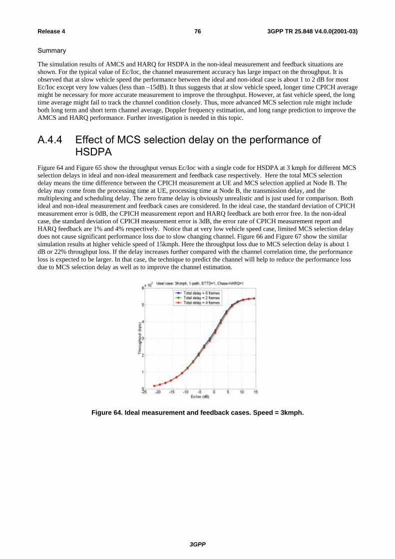
3GPP

3GPP TR 25.848 V4.0.0(2001-03)76Release 4

Summary

The simulation results of AMCS and HARQ for HSDPA in the non-ideal measurement and feedback situations are shown. For the typical value of Ec/Ioc, the channel measurement accuracy has large impact on the throughput. It is observed that at slow vehicle speed the performance between the ideal and non-ideal case is about 1 to 2 dB for most Ec/Ioc except very low values (less than –15dB). It thus suggests that at slow vehicle speed, longer time CPICH average might be necessary for more accurate measurement to improve the throughput. However, at fast vehicle speed, the long time average might fail to track the channel condition closely. Thus, more advanced MCS selection rule might include both long term and short term channel average, Doppler frequency estimation, and long range prediction to improve the AMCS and HARQ performance. Further investigation is needed in this topic.

A.4.4 Effect of MCS selection delay on the performance of HSDPA

Figure 64 and Figure 65 show the throughput versus Ec/Ioc with a single code for HSDPA at 3 kmph for different MCS selection delays in ideal and non-ideal measurement and feedback case respectively. Here the total MCS selection delay means the time difference between the CPICH measurement at UE and MCS selection applied at Node B. The delay may come from the processing time at UE, processing time at Node B, the transmission delay, and the multiplexing and scheduling delay. The zero frame delay is obviously unrealistic and is just used for comparison. Both ideal and non-ideal measurement and feedback cases are considered. In the ideal case, the standard deviation of CPICH measurement error is 0dB, the CPICH measurement report and HARQ feedback are both error free. In the non-ideal case, the standard deviation of CPICH measurement error is 3dB, the error rate of CPICH measurement report and HARQ feedback are 1% and 4% respectively. Notice that at very low vehicle speed case, limited MCS selection delay does not cause significant performance loss due to slow changing channel. Figure 66 and Figure 67 show the similar simulation results at higher vehicle speed of 15kmph. Here the throughput loss due to MCS selection delay is about 1 dB or 22% throughput loss. If the delay increases further compared with the channel correlation time, the performance loss is expected to be larger. In that case, the technique to predict the channel will help to reduce the performance loss due to MCS selection delay as well as to improve the channel estimation.

Figure 64. Ideal measurement and feedback cases. Speed = 3kmph.

3GPP

3GPP TR 25.848 V4.0.0(2001-03)77Release 4

Figure 65. Non-ideal measurement and feedback case. Speed = 3kmph.

Figure 66. Ideal measurement and feedback cases. Speed = 15kmph.

Figure 67. Non-ideal measurement and feedback case. Speed = 15kmph.

3GPP

3GPP TR 25.848 V4.0.0(2001-03)78Release 4

Summary:

The performance loss due to the MCS delay is not significant at very slow vehicle speed. However, it increases at higher vehicle speeds and for larger MCS selection delays. The channel prediction technique can be incorporated with the MCS selection rule to improve the AMCS and HARQ performance in HSDPA, especially at high speeds.

A.4.5 Integrated voice and data performance

Summary:

Sector data throughput of an integrated voice and High Speed Downlink Packet Access (HSDPA) system is investigated using the analytical-simulation approach described in [1]. The approach is to integrate the data throughput characteristic (Thruput(x)) in Equation 2 below obtained from link level simulations [2]) for a given channel condition with the achievable carrier to interference ratio (C/I (x)) obtained from system simulation for the coverage area of several representative sectors of the voice & data system.

Equation 2

∫−∗∗=

20

20)()( dxxPxThruputhruputAveSectorT

The predicted sector throughput is therefore calculated from a combination of link level and system simulations. Figure 68 shows the throughput in bps versus the ratio of energy per chip over other cell interference (Ec/Ioc) at the mobile receiver. We now use Ec/Ioc instead of C/I. Both Hybrid ARQ and transmit diversity (STTD) are enabled. Each curve plotted is in fact a composite of several link simulations for 64QAM R=3/4, 16QAM R=1/2 & R=3/4, and QPSK, using Turbo coding (see [2]). Hybrid ARQ in these simulations uses max-ratio combining of successive attempts (Chase combining). All curves have been simulated at 3kph one-ray Rayleigh fading channel model at a carrier frequency of 2GHz. Link adaptation switches between the modulation and coding levels to maximize the throughput for given Ec/Ioc value.

Single Code Throughput vs Ec/Ioc for HSDPA WCDMA

0

100000

200000

300000

400000

500000

600000

-30 -25 -20 -15 -10 -5 0 5 10 15 20

Ec/Ioc (dB)

Thro

ughp

ut (b

ps)

Figure 68. HSDPA Throughput Hull Curve vs Ec/Ioc for 3 kph and flat fading

The area probability for a given Ec/Ioc has been calculated from a system simulation of two hexagonal rings comprising 19 3-sector cells with log-normal standard deviation of 8.0dB and a 50% site to site correlation. A full set of radio (Eb/Nt vs FER) curves is used for modeling the 12.2kbit/s voice users. These curves account for 1,2, or 3rays with imbalances from 0 to 12 dB and speeds from 0 to 120kph and geometries (^Ior/Ioc) ranging from –6 to +12dB. The system is assumed to be 100% loaded resulting in the base transceivers having a constant 100% linear power amp (LPA) load of 17 Watts. By always transmitting with constant power (17 Watts in this case (see Figure 72) the voice

3GPP

3GPP TR 25.848 V4.0.0(2001-03)79Release 4

users will not see abrupt changes in interference levels as the available power margin is allocated to data. Of the LPA load, up to 70% of the power can be allocated to the data channel constructed from up to 20 (or 28) multicodes with spreading factor 32 depending on the voice users (12.2kbit/s) loading. The other 30% of the LPA load is allocated to overhead channels (such as pilot (CPICH), paging (PICH), synchronization (SCH), etc.) and dedicated control channels. The Ec/Ioc area distribution is based on the inner ring sectors and center cell sectors in order to exclude system edge effects .

The sector data throughput for “equal average power” scheduler may be calculated by integrating the throughput from the link simulations against the area pdf for Ec/Ioc derived from the system simulation (see Equations 2 below). The Ec/Ioc is determined from the available power margin left over after power is allocated to overhead channels (such as pilot (CPICH), paging (PICH), synchronization (SCH)), dedicated control channels, and voice user channels. The number of size 32 OVSF codes, and hence the peak rate that can be allocated, depends on the code tree left over after the overhead and voice channels have been allocated their codes. The equal average power scheduler assigns equal base station power to all users throughout the coverage area achieving the maximum possible throughput for each location. For HSDPA, equal average power scheduling would be achieved by cycling through all users in the coverage area, assigning one 3.33 ms frame with up to 20 (or 28) size 32 OVSF codes and up to 70% of the LPA power while using the optimum modulation and coding level. Over time, each user would receive an equal number of frames and therefore an equal average power allocation from the serving BTS. However, the average data received per user would be biased by the user’s location. Users closer to the base site would receive more data then those toward the cell edge.

Equation 3 (note the power margin could be up to 80% in the sytem simulation. Therefore, in the equations the computed Ec/Ioc is reduced by 0.6 dB to limit the maximum available power for HSDPA data to 70%)

Equation 3

tat time j cellfor )(

arg

arg

arg

jPP

PPPP

IE

cell

inm

ovhdvoiceinm

inm

or

c =++

=

),()(),()())((log101

10 kjTjPkiTiPIIIE

IE

cell

Ncells

icellonon

or

c

oc

c ∑=

=−⋅= λλ

klocation for ratiopower total tocell servingbest (FRP) recoveredpower available totaloffraction

klocation at mobile probe toi cell fromgain ion transmiss- Watts)17 (always j cellfor in Wattspower total- )(

−−

on

cell

I

T(i,k)jP

λ

)6.0(__ _ −−⋅= −− dBcodesmultioc

ccodesmulti N

IE

CurveHullThruputNThrupt

Conclusion:

Figure 69 below presents sector throughput of the equal average power scheduler for increasing voice loading and for different (FRP) fractions of total recovered power due to delay spread. For FRP=0.98 and 20 codes the achieved Data only Throughput is about 2.5Mbit/s which then drops almost linearly (see also Figure 70) as voice erlangs per sector increases. For a voice user (12.2kbit/s) load of about 35 erlangs/sector the Data ‘equal power’ sector throughput is still about 1Mbit/s.

An FRP of 0.98 results in about a 10% loss in throughput relative to an FRP=1.0 while a FRP of 0.92 results in about a 35% loss.

High data sector throughput is maintained by simply allocating the available power margin to data users. This approach is effective as long as the delay from measuring C/I and scheduling for a given user is small. Also the less slots (power control updates) a HSDPA frame encompasses the less margin needs to be set aside for voice users to guarantee them a minimum performance level during a scheduled burst. Alternatively, the power control rate for voice users could be reduced to 500Hz to minimize the power margin needed for voice users over a data frame interval such as 3.33ms.

The draw backs of the kind of simulation-analysis presented are that the effects of voice activity and fast FPC are not adequately modeled and such effects may degrade C/I estimation and hence degrade data throughput. Effects of voice

3GPP

3GPP TR 25.848 V4.0.0(2001-03)80Release 4

activity and fast FPC will be addressed in later analysis and future quasi-static system simulations. The reverse link will also be modeled.

Est. Achieved Data fwd link Throughput vs Voice Loading(Voice: STTD, FFPC Data: STTD, HARQ, FCS, 3.33ms Frame)

0

500000

1000000

1500000

2000000

2500000

3000000

0 5 10 15 20 25 30 35 40 45 50

Voice (Erlangs/Sector)

Thro

ughp

ut (b

ps)

stdev=8.0dB, lamda=1 stdev=8.0dB, lamda=0.98 stdev=8.0dB, lamda=0.95 stdev=8.0dB, lamda=0.92 .

System Layout: 2-ring 3sector PL = 128.1 +37log10(d), d is distance in km, ss dist=2800metersLogN Shadowing: stdev=8.0dB, ss corr=0.5, decor dist=100metersMax PA Power=17Watts, Effective VAF Uplink: 0.50 Downlink:0.55 No implementation loss on Voice link level curves or data thruput hull.Data channel: 3kph, Flat Fading, Max Ec/Ior=-1.6dBVoice channel: Users' speeds normal distirbution (m=30,std=15)kph

97% AreaCoverageReliabilityfor VoiceUp to 20 codes of size 32 allowed

MCS LevelsQPSK R=1/2, 16QAM R=1/2, R=3/4,64QAM R=3/4

Equi-probable (1,2,3 ray) multipath models with FRP (0.95), (0.80,0.12), (0.50 0.22 0.12)

Figure 69 HSDPA Throughput vs Voice Loading for different FRP (lamda) where an Equal Average Power Scheduler is assumed

0

500,000

1,000,000

1,500,000

2,000,000

2,500,000

3,000,000

3,500,000

0 5 10 15 20 25 30 35 40

Voice Erlangs per Sector

Avg

Sec

tor D

ata

Thro

ughp

ut (b

it/s)

lamda=1, <=20 codes lamda=1, <=28codeslamda=0.92, <=20 codes lamda=0.92, <=28 codes

MCS LevelsQPSK R=1/2, 16QAM R=1/2, R=3/4,64QAM R=3/4

System Layout: 2-ring 3sector PL = 128.1 +37log10(d), d is distance in km, ss dist=2800metersLogN Shadowing: stdev=8.0dB, ss corr=0.5, decor dist=100metersMax PA Power=17Watts, Effective VAF Uplink: 0.50 Downlink:0.55 No implementation loss on Voice link level curves or data thruput hull.Data channel: 3kph, Flat Fading, Max Ec/Ior=-1.6dBVoice channel: Users' speeds normal distirbution (m=30,std=15)kph Equi-probable (1,2,3 ray) multipath models with FRP (0.95), (0.80,0.12), (0.50 0.22 0 12)

Figure 70 HSDPA Throughput vs. Voice Loading for different FRP (lamda) and for 20 and 28 OVSF codes where and Equal Average Power Scheduler is assumed.

3GPP

3GPP TR 25.848 V4.0.0(2001-03)81Release 4

2200

4200

6200

8200

10200

12200

14200

3200 6850 10500 14150 17800x (meters)

y (m

eter

s)

Cell SiteSampling Pts

Figure 71 System used for Voice and Data HSDPA Simulation. C/I (Ec/Ioc) sampling points corresponding to coverage area of inner ring sectors and center cell sectors.

0%

10%

20%

30%

40%

50%

60%

70%

80%

90%

100%

1 2 3 4 5 6 7 8 9 10 11 12 13 14 15 16 17 18 19 20 21 22 23 24 25 26 27

time (20ms intervals)

17 W

att P

A p

ower

util

izat

ion

Pmargin

Pdch

Pvoice

Ppps

Figure 72 Percentage utilization of 17 Watt PA for a given sector in the system. Note at all times 17 Watts is transmitted for each sector.

3GPP

3GPP TR 25.848 V4.0.0(2001-03)82Release 4

A.4.6 Control information delay TPC commands for DL DPCH associated with HS-DSCH may be used to compensate for the DL channel condition

report delay and its fundamental ability is evaluated. A concept of the use of TPC commands is illustrated in Figure 73. TPC commands up to T_tx prior to transmission of HS-DSCH TUI are accumulated and used to adjust reported DL channel condition value. More generally, AMCS mode is selected based on DL channel quality estimated as below:

Equation 4

∑ −∆+=n

ncmdTPCTPCalphareportSIRSIRDL ])[_*21(**__

reportSIR _ is reported DL quality reported by UE, TPC∆ is UL power control step size applied, ][_ ncmdTPC is decoded power control command at slot n, and alpha is adjustment weight factor.

HS-DSCH sent on DL

TF of next DSCH frame sent on DL

4-TUI delay

CPICH measurement by UE T_meas

T_proc

T_tx

TUI: Transmission Unit Interval

T_dec

Measurement report sent on UL DPCH

T_enc

Power control commands used toadjust reported value

Figure 73 Use of power control commands for DL channel quality report adjustment

Figure 74 and Figure 75 shows the throughput gain achieved using TPC commands to adjust the DL channel quality report. T_tx is set to 4-slot for the evaluation with 3% error in TPC commands. TPC∆ is set to 1dB and alpha is set to 0.9375 in the simulation. For fading frequency up to 30Hz, gain over the hull characteristics can be achieved.

It must be noted that the gain shown here is dependent on T_tx. From throughput optimization and scheduling point of view, it is desirable to send control information (TF of HS-DSCH) aligned with the HS-DSCH TUI so that T_tx is minimized. On the other hand, for the receiver point of view, it is important that at least channelisation code information be received and decoded prior to receiving the first chip of the HS-DSCH TUI to avoid chip level buffering. Actual gain achievable by TPC adjustment needs to be re-evaluated after a decision is made on TF transmission scheme for HS-DSCH.

It also must be noted that unlike DSCH, DPCH may go into soft-handover state where TPC commands sent from UE does not fully represent DSCH link condition. Further studies need to be carried out to investigate if gain can be achieved in DPCH soft-handover case. Primary cell indicator for DSCH power control, which is in progress for Release 4 work item, may be used to correlate TPC with DSCH link condition .

Conclusions

Longer processing delay of 4 Transmission Unit Intervals (TUI) for DL channel quality report is considered for throughput analysis of HS-DSCH. When considering the control message format and timing for both UL and DL, impact to measurement delay must be kept in mind. It is shown that throughput degradation for 15~30Hz fading condition is significant compared with previous simulation assumption which only allowed 2 TUIs for reporting delay. As for now, a transmission scheme for control messages and expected delay associated with them have not been discussed in detail.

3GPP

3GPP TR 25.848 V4.0.0(2001-03)83Release 4

The following issues need to be clarified and studied:

- DL channel quality transmission scheme (Channel Type)

- Reporting rate and delay for DL channel quality with respect to HS-DSCH TUI

- HS-DSCH TF transmission scheme and associated delay

The document also showed some initial simulation results to indicate that use of accumulated TPC commands to adjust reported DL quality is effective to recover some of the throughput loss caused by reporting delay. Further study need to be carried out to validate its gain when associated DPCH is in soft-handover state.

Throughput Analysis: STTD, fd=6Hz, No ARQ

0

0.1

0.2

0.3

0.4

0.5

0.6

0.7

0.8

0.9

1

-20 -15 -10 -5 0 5 10

Ec/Nt (dB)

Nor

mal

ized

Thr

ough

put

delay=4 w/tpcdelay=4Hull


0

0.1

0.2

0.3

0.4

0.5

0.6

0.7

0.8

0.9

1

-20 -15 -10 -5 0 5 10Ec/Nt (dB)

Nor

mal

ized

Thr

ough

put



0

0.1

0.2

0.3

0.4

0.5

0.6

0.7

0.8

0.9

1

-20 -15 -10 -5 0 5 10

Ec/Nt (dB)

Nor

mal

ized

Thr

ough

put



0

0.1

0.20.3

0.40.5

0.60.70.8

0.91

-20 -15 -10 -5 0 5 10

Ec/Nt (dB)

Nor

mal

ized

Thr

ough

put


Figure 74 Delay compensation with TPC (No ARQ: TPC error rate=3%)

3GPP

3GPP TR 25.848 V4.0.0(2001-03)84Release 4

Throughput Analysis: STTD, fd=15Hz, H-ARQ=10

0

0.1

0.2

0.30.4

0.5

0.6

0.70.8

0.91

-20 -15 -10 -5 0 5 10

Ec/Nt (dB)

Nor

mal

ized

Thr

ough

put

delay=4 w/tpcdelay=4

Throughput Analysis: STTD, fd=30Hz, H-ARQ=10

0

0.1

0.2

0.3

0.4

0.5

0.6

0.7

0.8

0.9

1

-20 -15 -10 -5 0 5 10

Ec/Nt (dB)

Nor

mal

ized

Thr

ough

put

delay=4 w/tpcdelay=4

Figure 75 Delay compensation with TPC (ARQ=10: TPC error rate=3%)

3GPP

3GPP TR 25.848 V4.0.0(2001-03)85Release 4

Annex B: Examples of Performance Evaluation methods In the following, two examples of system performance evaluation methods are briefly described. First one is a combination of simulations and analytic evaluation and second one is based on dynamic system level simulations.

A. Analytic Simulation

In this method C/I statistics for all locations in a 19 cell, 3-sectored system is created and the corresponding C/I histogram is obtained. Next, from the link simulations the Throughput vs. C/I results are obtained for various MCS with STTD and Hybrid ARQ. The link and system simulation results are then combined and post-processed to obtain average sector throughput for various classes of scheduler. The flow diagram of this method is shown in Figure 8.

AverageSector Throughput

Get C/I samples from systemsimulation for a given Sector.

(Power level set to maximum with overhead, LognormalShadowing and Prop. model used)

Map C/I value into throughput("hull") curve to get a throughput

sample

Average throughput Samples

(weighting average allows different schedulingassumptions)

C/Ipdf

Thro

ughp

utpd

f

C/I

Throughput(bits/sec)

Figure 76. Analytic Simulation Flow Chart

In order to get an estimate of capacity the Max/Min scheduler as shown in Figure 9 is used. In this scheduler users with throughput above their own average get Max/Min more packets than users below the their own average.

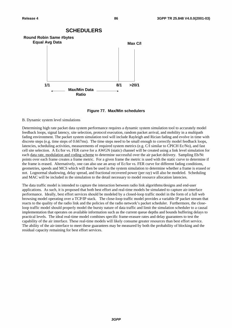
3GPP

3GPP TR 25.848 V4.0.0(2001-03)86Release 4

Figure 77. Max/Min schedulers

B. Dynamic system level simulations

Determining high rate packet data system performance requires a dynamic system simulation tool to accurately model feedback loops, signal latency, site selection, protocol execution, random packet arrival, and mobility in a multipath fading environment. The packet system simulation tool will include Rayleigh and Rician fading and evolve in time with discrete steps (e.g. time steps of 0.667ms). The time steps need to be small enough to correctly model feedback loops, latencies, scheduling activities, measurements of required system metrics (e.g. C/I similar to CPICH Ec/No), and fast cell site selection. A Ec/Ior vs. FER curve for a AWGN (static) channel will be created using a link level simulation for each data rate, modulation and coding scheme to determine successful over the air packet delivery. Sampling Eb/Nt points over each frame creates a frame metric. For a given frame the metric is used with the static curve to determine if the frame is erased. Alternatively, one can also use an array of Ec/Ior vs. FER curve for different fading conditions, geometries, speeds and MCS which will then be used in the system simulation to determine whether a frame is erased or not. Lognormal shadowing, delay spread, and fractional recovered power (per ray) will also be modeled. Scheduling and MAC will be included in the simulation to the detail necessary to model resource allocation latencies.

The data traffic model is intended to capture the interaction between radio link algorithms/designs and end-user applications. As such, it is proposed that both best effort and real-time models be simulated to capture air-interface performance. Ideally, best effort services should be modeled by a closed-loop traffic model in the form of a full web browsing model operating over a TCP/IP stack. The close-loop traffic model provides a variable IP packet stream that reacts to the quality of the radio link and the policies of the radio network’s packet scheduler. Furthermore, the close-loop traffic model should properly model the bursty nature of data traffic and limit the simulation scheduler to a causal implementation that operates on available information such as the current queue depths and bounds buffering delays to practical levels. The ideal real-time model combines specific frame-erasure rates and delay guarantees to test the capability of the air interface. These real-time models will likely consume greater resources than best effort service. The ability of the air-interface to meet these guarantees may be measured by both the probability of blocking and the residual capacity remaining for best effort services.

1/1 8/1

Equal Avg Data

SCHEDULERSRound Robin Same #bytes

Max/Min DataRatio

>20/1

Max C/I

3GPP

3GPP TR 25.848 V4.0.0(2001-03)87Release 4

Annex C: Throughput Metric Definitions OTA – over the air per frame throughput, Frame Rate/#transmissions. (Unaffected by time between retries.)

Service – total good (successful) frame bits transmitted per second for a given sector. As observed from BTS including all users and idle time. (Affected by time between retries).

Packet Call - total bits per packet call divided by total time to transmit packet call.

Utilization – percentage of time that frame intervals are active for a given sector.

(active = transmission occurs on downlink shared channel).

Retry 2Retry 1First Tx)(

)(im

R(i)iOTA =

∑∑==

=framesgoodframesgood N

i

N

i

imiROTA__

11

)()(

(Averaged over all users)

k sec k+1 sec

. . .

No Tx Bad FrameGood Frame

frame intervals

user)any (for interval second kth in bits good#)( =kService

onds

N

k

N

kServiceService

onds

sec

1

sec

)(∑==

(per sector)

tk tend_k

frame intervals

)k callpkt in bits# )(

_ karrivalend_k t(tkPktCall

−=

PktCalls

Npktcalls

m

N

mPktCallPacketCall

∑== 1

)(

(Averaged using all users’ packetcalls)

Good FramePacket Call k

frame intervals

ith frame withrate R(i) forUser A

Tx frames forgiven sector

tarrival_k

(in Queue)

User A’s PacketCall k

BadFrame

Good Frame

BadFrame

No Tx

Figure 78 Throughput Statistic Description for System Simulations

The service throughput for a given sector j is

∑=

=ondsN

kondsNjtorServiceSec

sec

1sec

jsector for inverval secondkth for bits good#1)( Equation 5

3GPP

3GPP TR 25.848 V4.0.0(2001-03)88Release 4

The service throughput averaged over all sectors in the system is ∑=

=torsN

jtors

jtorServiceSecN

temServiceSyssec

1sec

)(1

Equation 6

Also

torsonds NNtemServiceSys

secsec

sectors all bits good total= Equation 7

or

frameemptyretriesframesgood TNNNtemServiceSys

)(sectors all bits good total

_ ++= Equation 8

where

Ngood_frames – total good frames over all sectors sent during simulation Nretries – total unsuccessful (“bad”) frames over all sectors transmitted during simulation Nempty – total frame intervals over all sectors where there was no transmission during sim. Nlost – total frame intervals over all sectors where the corresponding frame was aborted during sim. Tframe – frame time interval

frameretriesframesgood TNNOTASystem

)( _ +=

users all bits good total Equation 9

lostemptyretriesframesgood

lostretriesframesgood

NNNNNNN

nUtilizatio+++

++=

_

_ Equation 10

emptyretriesframesgood

retriesframesgood

NNNNN

OTASystemtemServiceSys

++

+=

_

_ Equation 11

Therefore

OTASystemtemServiceSysnUtilizatio ≈ Equation 12

The packet call throughput is given by

)(k callpkt in bits#),,(

__ karrivalkend ttjikPktCall

−= Equation 13

where

k = denotes the kth packet call from a group of K packet calls i = denotes the ith user from a group of N users j = denotes the jth drop from a group of J drops the time parameters in Equation 10 are described in Figure A1. The user packet call throughput becomes

∑=

=K

kjikPktCall

KjilUserPktCal

1),,(1),( Equation 14

3GPP

3GPP TR 25.848 V4.0.0(2001-03)89Release 4

Annex D: Change history

Change history Date TSG # TSG Doc. CR Rev Subject/Comment Old New

16/03/01 RAN_11 RP-010191 - - Approved at TSG RAN #11 and placed under Change Control - 4.0.0

technical report - 株式会社qt · this tr describes the physical layer aspect of the techniques...

Documents