TGV for diffusion tensors: A comparison of fidelity functions

Tuomo Valkonen*, Kristian Bredies and Florian Knoll§

October 24, 2012

Abstract

We study the total generalised variation regularisation of symmetric tensor fields from medicalapplications, namely diffusion tensor regularisation. We study the effect of the pointwise positivityconstraint on the tensor field, as well as the difference between direct denoising of the tensor fieldfirst solved from the Stejskal-Tanner equation, as was done in our earlier work, and of incorporatingthis equation into the fidelity function. Our results indicate that the latter novel approach providesimproved computational results.

Mathematics subject classification: 92C55, 94A08, 26B30, 49M29.

Keywords: total generalised variation, total deformation, regularisation, diffusion tensor imag-ing, medical imaging.

1 Introduction

In this manuscript, we present a numerical study of total generalised variation (TGV) regularisation[6] of second-order symmetric tensor fields u ∈ L1(Ω; Sym2(Rm)), namely the problem

minu≥0

1

2‖f −Au‖2 + TGV`

~α(u), (P)

where we have a pointwise a.e. positive semi-definiteness constraint on u. The measurement f ∈L1(Ω;X) for a finite-dimensional Hilbert space X, and the operator A is the pointwise superpositionoperator associated with a linear operator A : Sym2(Rm) → X, where the tensor space Sym2(Rm)consists of symmetric bilinear mappings on Rm×Rm. The TGV` regularisation functionals extended totensor fields employ the symmetrised distributional derivative Eu of u instead of the full derivative Duin order to obtain weaker gradient information. The former, which we have found to produce improveddenoising results [23], may for u ∈ C1(Ω; Sym2(Rm)) be formally written as Eu = (Du + (Du)T )/2.For symmetric tensor fields of bounded deformation the distribution Eu is a measure with values inSym3(Rm), i.e., third-order symmetric tensors. First order TGV, also called total deformation or TD,thus reads

TGV1α(u) := αTD(u) := α‖Eu‖F,M(Ω;Sym3(Rm))

where ‖ · ‖F,M(Ω;Symk(Rm)) is the Radon norm. Solutions to first-order regularisation problem tend toexhibit staircasing artefacts, as we will also see in the numerical experiments that we perform in thispaper. In order to reduce these effects, we employ second-order total generalised variation TGV2 [6],which for symmetric tensor fields reads

TGV2(β,α)(u) := min

w∈L1(Ω;Sym3(Rm))α‖Eu− w‖F,M(Ω;Sym3(Rm)) + β‖Ew‖F,M(Ω;Sym4(Rm)).

*Institute for Mathematics and Scientific Computing, University of Graz, Austria. tuomo.valkonen@iki.fiNow at Department of Applied Mathematics and Theoretical Physics, University of Cambridge, United Kingdom.Institute for Mathematics and Scientific Computing, University of Graz, Austria. kristian.bredies@uni-graz.at§Institute of Medical Engineering, Graz University of Technology, Austria. florian.knoll@tugraz.at

1

The main motivation for considering the problem (P) is diffusion-weighted magnetic resonance imaging(DWI, diffusion MRI) which images a tensor field g describing the anisotropic diffusion of watermolecules, providing insight into the white matter structure of the brain [3, 21] with the objectiveof performing medical diagnosis. Diffusion-weighted MRI has long acquisition times, even with ultrafast sequences like echo planar imaging (EPI). It is therefore a low-resolution and low-SNR method,exhibiting Rician noise [13] and eddy-current distortions [21]. It is, moreover, very sensitive to patientmotion [14, 1]. It is therefore of utmost importance to denoise the diffusion tensor field g. Variousapproaches are reviewed in [23], with the focus on the direct denoising of g by (P) with A = I theidentity, X = Sym2(R3), and f = g. As in DWI, the (noisy) tensor field is not measured directly,we have to assume that g is already given as the outcome of some reconstruction process. Undersuch an assumption, we showed that TGV2, first introduced in [6] for scalar fields, as well as totaldeformation (TD), both based on the symmetrised gradient, offer superior denoising performance overother evaluated approaches. These include total variation (TV) [18], and “logarithmic TV” [11], whichis based on log-Euclidean metrics [2].

In this paper, we incorporate the above-mentioned reconstruction process into the denoising prob-lem. Let, for i = 0, . . . ,K be the varying diffusion gradients bi ∈ R3 associated with the DWImeasurement, including the zero gradient b0 = 0. The measured data then consists of si ∈ L1(Ω)(i = 0, . . . ,K), which is related to the sought diffusion tensor field u ∈ L1(Ω; Sym2(R3)) via theStejskal-Tanner equation [3, 15]

si = s0 exp(−〈bi ⊗ bi, u〉). (1.1)

If bi⊗ bi form a (necessarily non-orthogonal) basis of Sym2(R3), we may solve this equation for u. Wewant to see what effect incorporating (1.1) into (P) has. However, in order to get a linear inversionproblem, we reformulate the Stejskal-Tanner equation. Observe that

log(si/s0) + 〈bi ⊗ bi, u〉 = 0.

Therefore, with X = RK , setting

f =(log(s1/s0), . . . , log(sK/s0)

)(1.2)

and (Au)(x) = Au(x) for x ∈ Ω where

Av =(−〈b1 ⊗ b1, v〉, . . . ,−〈bK ⊗ bK , v〉

), (1.3)

we have a problem of the form A(u) = f . As the measurements si are noisy, we choose to regularisewith TGV`

~α(u) which leads to a problem of type (P). We will compare this against the approach of[23] for both TGV2, and TGV1, the latter agreeing with total deformation (TD). We moreover studythe effect of the pointwise positivity constraint u ≥ 0.

The solution of the positivity constrained problem (P) poses some numerical challenges. We employthe Chambolle-Pock method [9], which is a first-order method for solving saddle-point problems of theform

minu

maxφ

G(u) + 〈Ku, φ〉 − F ∗(φ). (1.4)

With the reformulation of (P) in the form (1.4) that was employed in [23], the computational hotspotof the algorithm is the computation on each iteration of the resolvent (I + τ∂G)−1(y) of

G(u) :=1

2‖f −Au‖2 + δ≥0(u), (1.5)

where the indicator function δ≥0 replaces the pointwise positivity constraint. In the case A = I, thecalculation of the resolvent amounts to pointwise projection of a second-order tensor to the positivesemi-definite cone. This is computationally demanding, as in practise the QR algorithm is requiredfor numerical stability. Nevertheless, the overall method has turned out to be reasonably efficient,minding the non-smooth nature of the problem, which complicates the application of second-order

2

methods. For the case (1.2), (1.3), we have A 6= I, and sticking to the same approach, to compute theresolvent, we have to perform “weighted projections”

min0≤X∈Sym2(Rm)

‖AX − c‖2, (1.6)

which are more demanding to solve. We have developed a novel simple and efficient interior pointmethod for this projection in [22]. We have, however, experimentally observed that the Chambolle-Pock method itself has poor convergence when A∗A is far from proportional to the identity and G asin (1.5). We therefore introduce an additional dual variable and write (P) in an alternative way inthe same form (1.4). Although this formulation has poorer theoretical convergence properties, lackinguniform convexity, and indeed does not provide extremely fast convergence, it appears to providebetter convergence than our earlier formulation when A∗A is far from proportional to the identity.

The rest of this paper is organised as follows. In Section 2 we introduce the tensor and tensor fieldcalculus to set up the framework in which our results are represented. Then in Section 3 we formulatethe problem (P) in detail. Section 4 describes our numerical method for the solution of (P). Then,in Section 5 we study the performance of our method. We finish the paper with our conclusions inSection 6.

2 Tensors and tensor fields

We now recall basic tensor calculus, as needed for the development of TGV2. We make many sim-plifications, as, working on the Euclidean space Rm, it would not serve our purposes the employ andintroduce the machinery in its full differential-geometric setting [4].

Basic tensor calculus By a k-tensor A ∈ T k(Rm) we mean a k-linear mapping A : Rm × · · · ×Rm → R. A symmetric tensor A ∈ Symk(Rm) satisfies for any permutation π of 1, . . . , k thatA(cπ1, . . . , cπk) = A(c1, . . . , ck) for all c1, . . . , ck ∈ Rm. We will only need symmetric tensors in thiswork. With e1, . . . , em the standard basis of Rm, we define the inner product

〈A,B〉 :=∑

p∈1,...,mkA(ep1 , . . . , epk)B(ep1 , . . . , epk),

and the induced Frobenius norm‖A‖F :=

√〈A,A〉.

Example 2.1. We observe that 1-tensors can be identified with vectors A ∈ Rm by defining A(x) =〈A, x〉. (Strictly speaking the vector A is the holor of the tensor defined this way.) The inner productis the usual inner product in Rm, and the Frobenius norm ‖A‖F = ‖A‖2. Likewise 2-tensors canbe identified with matrices A ∈ Rm×m by defining A(x, y) = 〈Ax, y〉. Symmetric matrices A = AT

give rise to symmetric 2-tensors. The inner product is 〈A,B〉 =∑

i,j AijBij and ‖A‖F is the matrixFrobenius norm.

Symmetric tensor fields Let u : Ω→ Symk(Rm) for a domain Ω ⊂ Rm. We then set

‖u‖F,p :=(∫

Ω‖u(x)‖pF dx

)1/p, (p ∈ [1,∞)), and ‖u‖F,∞ := ess supx∈Ω ‖u(x)‖F

as well as the abbreviation ‖ · ‖ = ‖ · ‖F,2, and define the spaces

Lp(Ω; Symk(Rm)) = u : Ω→ Symk(Rm) | ‖u‖F,p <∞, (p ∈ [1,∞]).

3

For u ∈ C1(Ω; Symk(Rm)), k ≥ 1, we define the divergence div u ∈ C(Ω; Symk−1(Rm)) by contrac-tion as

[div u(x)](ei2 , . . . , eik) :=m∑i1=1

∂i1 [x 7→ u(x)(ei1 , . . . , eik)]

=m∑i1=1

〈ei1 ,∇u(·)(ei1 , . . . , eik)〉.(2.1)

Observe the operator div preserves symmetricity.

Example 2.2. If u ∈ C1(Ω;Rm) = C1(Ω; T 1(Rm)) is a vector field, then div u(x) =∑m

i=1 ∂iui(x)is the usual divergence. If u ∈ C1(Ω; T 2(Rm)), then [div u(x)]j =

∑mi=1 ∂iuij(x). That is, we take

columnwise the divergence of a vector field.

The symmetrised gradient Denoting by X∗ the continuous linear functionals on the topologicalvector space X, we now define the symmetrised distributional gradient

Eu ∈ [C∞c (Ω; Symk+1(Rm))]∗

of u ∈ L1(Ω; Symk(Rm)) by

Eu(ϕ) := −∫

Ω〈u(x), divϕ(x)〉 dx, (ϕ ∈ C∞c (Ω; Symk+1(Rm))).

Let us also define the “symmetric Frobenius unit ball”

V kF,s := ϕ ∈ C∞c (Ω; Symk(Rm)) | ‖ϕ‖F,∞ ≤ 1.

If supEu(ϕ) | ϕ ∈ V k+1F,s <∞, then Eu is a measure [10, §4.1.5]. Indeed, for our purposes it suffices to

define a tensor-valued measure µ ∈M(Ω; Symk(Rm)) as a linear functional µ ∈ [C∞c (Ω; Symk(Rm))]∗

bounded in the sense that the total variation norm

‖µ‖F,M(Ω;Symk(Rm)) := supµ(ϕ) | ϕ ∈ V kF,s <∞.

Example 2.3. For smooth vector fields u ∈ C∞(Ω;Rm), we have Eu = EuLm, where Eu(x) :=(∇u(x) + (∇u(x))T )/2 is the pointwise symmetrisation of the usual gradient, and Lm denotes theLebesgue measure; cf. [20]. For scalar fields u ∈ L1(Ω), the symmetrised gradient is the usual distri-butional gradient, Eu = Du.

Miscellaneous notation We denote by

δM (x) :=

0, x ∈M,

∞, x 6∈M,

the indicator function of a set M in the sense of convex analysis, and particularly by

δ≥0(u) :=

0, u(x) is positive semi-definite for a.e. x ∈ Ω,

∞, otherwise,

the indicator function of the pointwise positive semi-definite cone. We use the notation u ≥ 0 forpointwise a.e. positive semi-definite u ∈ L1(Ω; Sym2(Rm)).

3 Total generalised variation of tensor fields

We now develop first- and second-order total generalised variation for tensor fields.

4

Total deformation (TGV1) We define the first-order total generalised variation or total deforma-tion of a tensor field u ∈ L1(Ω; Symk(Rm)) simply by

TD(u) := ‖Eu‖F,M(Ω;Symk+1(Rm)) = supϕ∈V k+1

F,s

∫Ωu(x) divϕ(x) dx.

Observe that we bound ϕ pointwise by the Frobenius norm. The reason for this is that we desirerotation-invariance: for details see [23].

As already remarked, in the case of scalar fields u ∈ L1(Ω; Sym0(Rm)) ∼ L1(Ω), i.e., k = 0, we haveEu = Du, so that TD = TV. For k = 1, i.e., vector fields u ∈ L1(Ω; Sym1(Rm)) ∼ L1(Ω;Rm), thefunctional TD agrees with the total deformation of [20]. We can also define tensorial total variationper TV(u) := ‖Du‖F,M(Ω;T k+1(Rm)) where Du is the usual distributional derivative of u. This is donein [23], where we observe that TD provides better regularisation results.

We also denote TGV1α := αTD, because total deformation is the first-order version of TGV.

Moreover, we consider a fixed linear mapping A : Sym2(Rm)→ X for a Hilbert space X and denote,again, by A the corresponding pointwise superposition operator. The problem (P) may thus be writtenin inf-sup form

minv

supξG(v) + 〈v,K∗ξ〉 − F ∗(ξ) (S)

with the unknowns

v := u ∈ L1(Ω; Sym2(Rm)),

ξ := ϕ ∈ C∞c (Ω; Sym3(Rm)),

and the functionals

G(u) :=1

2‖f −Au‖2 + δ≥0(u),

K∗ϕ := −divϕ, and (S-TD)

F ∗(ϕ) := δαV 3F,s

(φ).

The conjugate-like notation K∗ will be justified in Section 4.Alternatively, we may introduce, as for instance in [5], an additional dual variable λ, and write

1

2‖f −Au‖2 = sup

λ〈λ,Au− f〉2 − 1

2‖λ‖2. (3.1)

Then with the unknowns

v := u ∈ L1(Ω; Sym2(Rm)),

ξ := (ϕ, λ) ∈ C∞c (Ω; Sym3(Rm))× L1(Ω; Sym2(Rm))

we set

G(u) := δ≥0(u),

K∗(ϕ, λ) := (−divϕ+A∗λ), and (S-TD-alt)

F ∗(ϕ) := δβV 3F,s

(ψ) +1

2‖λ‖2 + 〈f, λ〉.

Second-order total generalised variation (TGV2) Second-order total generalised variation, in-troduced in [6], tends to avoid [16] the stair-casing effect of first-order regularisation models. Givenparameters ~α = (α, β) > 0, we now define it for tensor fields u ∈ L1(Ω; Symk(Rm)) by the differentia-tion cascade

TGV2~α(u) := min

w∈L1(Ω;Symk+1(Rm))α‖Eu− w‖F,M(Ω;Symk+1(Rm)) + β‖Ew‖F,M(Ω;Symk+2(Rm)). (3.2)

5

It is shown in [7, 8] that this formulation is for scalar fields k = 0 equivalent to the original dual-ballformulation in [6]. We choose to use the formulation (3.2) directly because it is more practical fornumerical realisation, simplifying constraints through a kind of variable splitting.

The problem (P) for ` = 2 may again be written in the inf-sup form (S) with the unknowns

v := (u,w) ∈ L1(Ω; Sym2(Rm))× L1(Ω; Sym3(Rm)), and

ξ := (ϕ,ψ) ∈ C∞c (Ω; Sym3(Rm))× C∞c (Ω; Sym4(Rm)),

and the functionals

G(u,w) :=1

2‖f −Au‖2 + δ≥0(u),

K∗(ϕ,ψ) := (−divϕ,−ϕ− divψ), and (S-TGV2)

F ∗(ϕ,ψ) := δαV 3F,s

(ϕ) + δβV 4F,s

(ψ).

Alternatively, we may do as in (3.1), and with the unknowns

v := (u,w) ∈ L1(Ω; Sym2(Rm))× L1(Ω; Sym3(Rm)), and

ξ := (ϕ,ψ, λ) ∈ C∞c (Ω; Sym3(Rm))× C∞c (Ω; Sym4(Rm))× L1(Ω; Sym2(Rm))

write

G(u,w) := δ≥0(u),

K∗(ϕ,ψ, λ) := (−divϕ+A∗λ,−ϕ− divψ), and (S-TGV2-alt)

F ∗(ϕ,ψ, λ) := δαV 3F,s

(ϕ) + δβV 4F,s

(ψ) +1

2‖λ‖2 + 〈f, λ〉.

4 The numerical method

We now move on to discuss the algorithmic aspects of the solution of the regularisation problemsabove. We do this through the min-sup formulations.

Discretisation and the algorithm We intend to apply the Chambolle-Pock algorithm [9] to theinf-sup problem (S) for the functionals (S-TD), (S-TD-alt), (S-TGV2), and (S-TGV2-alt). Thiscan be done after we discretise the original problem first; for the infinite-dimensional problem the(pre)conjugate K of K∗ is not well-defined. We represent each tensor field f , u, w, ϕ and ψ withvalues on a uniform rectangular grid Ωh of cell width h > 0, and discretise the operator div by forwarddifferences with zero boundary conditions as divh. We choose not to use central differences, becauseit tends to cause oscillation in this problem. The operator A∗ is discretised in the straightforwardmanner as pointwise application of A∗ on the grid points. This yields the discretised version K∗h ofthe operator K∗. We then take Kh := (K∗h)∗ as the discrete conjugate of K∗h.

We also like to employ the acceleration strategies for the primal-dual algorithm in [9]. Assumingthat the operator A has full rank, observe that G for TD as given in (S-TD), is uniformly convex inu in the sense that there exists a factor γ > 0 (dependent on A) such that for any u′ it holds

G(u′)−G(u) ≥ 〈z, u′ − u〉+γ

2‖u− u′‖2 for all z ∈ ∂G(u), x′ ∈ X.

This implies that acceleration can be employed. The alternative formulations (S-TD-alt) for TD, and(S-TGV2-alt) for TGV2, however, are not uniformly convex, so γ = 0. For TGV2, the functionalG as given in (S-TGV2), is uniformly convex in u, but not in w. We should therefore take γ = 0in the algorithm below, although in numerical practise taking γ as the factor of uniform convexitywith respect to u alone, sometimes offers faster convergence, at other times however failing to exhibitconvergence.

6

Algorithm 4.1. Perform the steps:

1. Pick τ0, σ0 > 0 satisfying τ0σ0‖Kh‖2 < 1, as well as initial iterates (v0, ξ0). Set v0 = v0. Let γbe the factor of uniform convexity of G.

2. For i = 0, 1, 2, . . ., repeat until a stopping criterion is satisfied.

ξi+1 := (I + σi∂F∗)−1(ξi + σiKhvi)

vi+1 := (I + τi∂G)−1(vi − τiK∗hξi+1)

θi := (1 + 2γτi)−1/2, τi+1 := θiτi, σi+1 := σi/θi

vi+1 := vi+1 + θi(vi+1 − vi).

Here, (I + σ∂F ∗)−1 and (I + τ∂G)−1 are resolvent mappings associated with the subgradients ofF ∗ and G, respectively, for details see [17], for instance.

Calculating the resolvents We now study how to calculate for (S-TGV2) the resolvents (I +τ∂G)−1(v) and (I + σ∂F ∗)−1(ξ), which are needed to obtain ξi+1 and vi+1 in Algorithm 4.1. Thesolution for (S-TD) is then a simplified version. For (S-TD-alt) and (S-TGV2-alt) the resolvent (I +τ∂G)−1(v) is likewise a simplified version of the case considered below, while (I+σ∂F ∗)−1(ξ) amountsin each case to simple pointwise operations on ξ, which have already been discussed in the literature;for instance, see [23, 5].

The resolvents have the expressions

(I + τ∂G)−1(v) = arg miny

‖v − y‖2

2τ+G(y)

,

where for pairs v = (u,w) we have to take ‖v‖2 = ‖u‖2+‖w‖2. The efficient realisation of Algorithm 4.1depends on the efficient realisation of these minimisation problems. As discussed in [23], calculation of(I+σ∂F ∗)−1(ϕ,ψ) reduces to pointwise projection of ϕ to the ball αV 3

F,s and of ψ to αV 4F,s. Moreover,

for (S-TD-alt) and (S-TGV2-alt), λ is mapped to (λ−σf)/(1+σ). The calculation of (I+τ∂G)−1(u,w)for (S-TD) and (S-TGV2) is more demanding. Recalling that

G(u,w) =1

2‖f −Au‖22 + δ≥0(u),

we find that(u,w) = (I + τ∂G)−1(v, q)

satisfy w = q, and that u(x) for each x ∈ Ω is the solution of

(I + τA∗A)u(x) +N≥0(u(x)) 3 v(x) + τA∗f(x). (4.1)

Here N≥0(u(x)) is the normal cone of the positive semi-definite cone at u(x). If A = I, this simplifiesto

(1 + τ)u(x) +N≥0(u(x)) 3 v(x) + τf(x),

so that

u(x) = P≥0

(v(x) + f(x)τ

1 + τ

).

The projection P≥0 to the positive definite cone can be calculated by performing eigen-decompositionusing QR algorithm, see [12] for details. This is also true for (S-TD-alt) and (S-TGV2-alt) in which casethe resolvent is just the projection on the positive definite cone. If A 6= I, then writing M = I+ τA∗Aand C = v(x) + τA∗f(x), the problem (4.1) can be stated in terms of X = u(x) ∈ Sym2(Rm) and adual variable S ∈ Sym2(Rm) as

MX − S = C, (XS + SX)/2 = 0, X, S ≥ 0. (4.2)

7

This system of equations can be approximately solved in a low number of steps with the novel primal-dual interior point algorithm of [22].

Finally, we remark that when we do not include the positivity constraint (P), then the projectionsabove may be skipped, and instead of (4.1), we simply solve u(x) from

Mu(x) = C.

Stopping criterion For (S-TD) and (S-TD-alt), we use the fractional duality gap as stoppingcriterion. Namely we stop execution of Algorithm 4.1 if a preset maximum number of iterations isreached, or for a given target fractional duality gap ρ ∈ (0, 1), we have Di/D0 < ρ, where the dualitygap

Di := F (Khvi) +G(vi) +G∗(−K∗hξi) + F ∗(ξi). (4.3)

For (S-TGV2) and (S-TGV2-alt) we cannot use this as such, because often simply Di =∞ due to theindependence of G from w. In [23] we have shown that by including in G the term M‖w‖F,1, for an aposteriori chosen M > 0, we can use the resulting “pseudo-duality gap” as a stopping criterion.

5 Numerical results

Experimental setup We apply the regularisation models discussed above to a clinical in-vivo dif-fusion tensor image of a human brain. The measurements for our test data set were performed on aclinical 3T system (Siemens Magnetom TIM Trio, Erlangen, Germany), using a 32 channel head coil.Written informed consent was obtained from all volunteers before the examination. A 2D diffusionweighted single shot EPI sequence with diffusion sensitising gradients applied in 12 independent direc-tions (b = 1000s/mm2) and an additional reference scan without diffusion was used with the followingsequence parameters: TR = 7900ms, TE = 94ms, flip angle 90, matrix size 128× 128, 60 slices witha slice thickness of 2mm, in plane resolution 1.95mm × 1.95mm, 4 averages, GRAPPA accelerationfactor 2. The exact measurement time of the entire sequence is 7 minutes and 22 seconds. Prior tothe reconstruction of the diffusion tensor, eddy current correction was performed with FSL [19].

We perform computations only on slice 23 of the data set. As a ground truth, we construct the dif-fusion tensor image g0 by the Stejskal-Tanner equation (1.1) from all the 52 (4 averages of 12+1) DWImeasurements s = (s0, . . . , s51). We then take only the 7 measurements s = (s0, s2, s4, s5, s6, s8, s11),containing one zero diffusion gradient and six independent gradients. The six independent gradi-ents are chosen among all the 12 to minimise the condition number of the operator A∗A, where Ais constructed by (1.3). From the reduced data set s we construct a lower-quality image g by theStejskal-Tanner equation. This kind of reduction of the number of measurements would bring thescanning time from the 7 minutes and 22 seconds to below 2 minutes, which would be beneficial toreduce artefacts from patient motion and improve patient comfort.

We denoise g directly by minimising ‖g − u‖2 with both TGV2 and TD regulariser, with andwithout the positivity constraint. We call this the “direct denoising problem”, as we are directlyminimising the distance between two tensor fields subject to regularisation and constraints. We alsodenoise g “indirectly” by minimising ‖f −Au‖2, where f and A are as in (1.2) and (1.3), respectively.We again use both TGV2 and TD as regulariser, both with and without the positivity constraint. Wecall this the “raw DWI-based denoising problem”, because the fidelity function incorporates the DWImeasurements through the Stejskal-Tanner equation.

We compute the denoising result of every model for all the regularisation parameters

α ∈ 0.0003, 0.0006, 0.0009, 0.0012, 0.0015, 0.0018, 0.0021, 0.0024, 0.0027,

0.00003, 0.00006, 0.00009, 0.00012, 0.00015, 0.00018, 0.00021, 0.00024, 0.00027.

For TGV2 we take β = α. This range was chosen by trial and error to yield qualitatively goodresults and also be large enough such that when we calculate for each α the Frobenius norm error‖χbrain(u− g0)‖F,2 to the ground-truth g0, then the optimal α, yielding smallest error, lies inside this

8

range, not on the boundary. Here χbrain : Ω → 0, 1 is the brain mask, defined as excluding pointswhere the average DWI signal intensity is less than 10% of the mean over the whole image. In thecomparisons that we now get into, for each model we report the result for the optimal choice of α. Allthe reported error scores also use the mask χbrain, and the corresponding area has been masked outin the visualisations, to avoid displaying distractive noise outside the imaged brain.

Performance considerations between formulations We use for all Algorithm 4.1 for all com-putations. For the situation A = I, i.e., the direct denoising problem, the formulations (S-TD) and(S-TGV2) are faster convergent than the formulations (S-TD-alt) and (S-TGV2-alt) with the extradual variable λ. Indeed, by the uniform convexity of (S-TD), Algorithm 4.1 has O(1/N2) convergencerate [9]. This still holds for A 6= I, i.e., the raw DWI-based denoising problem, but in practise wehave observed that if the operator A is far from orthogonal, although initial convergence is fast, thealgorithm quickly becomes slowly convergent without having reached a high-quality solution. Thishappens both with and without the positivity constraint. In most situations we have found the targetfractional duality gap ρ = 0.001 to offer reasonable solutions. This is also the case for the current“optimal” choice of the six independent diffusion gradients (with condition number ∼6.8 for A∗A). If,however, we picked the 6 first independent diffusion gradients, i.e., set s = (s0, . . . , s7) (which yieldscondition number ∼33.6 for A∗A), we have found that we would need at least ρ = 0.00001 to get rea-sonable solutions with the formulations (S-TD) and (S-TGV2). This results in higher computationaltimes. We note, however, that although the effect is less extreme, the formulations (S-TD-alt) and(S-TGV2-alt) also exhibit diminished convergence speeds in this case (ρ = 0.001 giving red tone in theprincipal eigenvector plots), suggesting that the whole raw DWI-based denoising problem has widerproblems with A∗A not being the identity.

In the positivity constrained case there are also some additional numerical difficulties with theformulations (S-TD) and (S-TGV2). Although the interior point algorithm of [22] can in few iterationsfind an approximate solution (fractional duality gap < 0.001) to (4.2), and this is sufficient to obtaingood solutions with Algorithm 4.1, such approximate solutions are not sufficiently good for calculatingthe fractional duality gap (4.3) for use as a stopping criterion in Algorithm 4.1. Namely, in order tocalculate the duality gap, we need to compute a high-quality approximation of the conjugate

G∗(q) := supu〈q, u〉 −G(u).

This also involves the solution of (4.2). When we calculate the solution only approximately, G∗ andthen consequently the duality gap ends up computed too small, causing early termination of theAlgorithm 4.1, or none at all, when the initial duality gap is computed too small. Thus we presentlyhave to compute the solution to (4.2) very exactly, which results in rather long running times. Thehigher condition number of A∗A also increases the running times, as the complexity of the interiorpoint method depends on the condition number. Alternatively we should not use the duality gap asstopping criterion, and simply run Algorithm 4.1 for a fixed number of iterations.

The above performance considerations have led us to the following conclusions. For the directdenoising problem, we employ the formulations (S-TD) and (S-TGV2). For the raw DWI-baseddenoising problem, we employ the alternative problem formulations (S-TD-alt) and (S-TGV2-alt)if A∗A is far from the identity. For A from the present experimental setup (with the optimal choiceof the independent diffusion gradients), the Chambolle-Pock algorithm however converges fast for theformulations (S-TD) and (S-TGV2), so we use them. Due to the problems with the exact calculation ofthe duality gap, the run time of the method (in seconds) is however not comparable for the constrainedraw DWI-based fidelity to the other fidelities.

Quantitative results We set the target fractional duality gap ρ = 0.001 and a maximum itera-tion count 5000. With this choice, error scores for the computational results for the optimal α arereported in Table 1. In addition to the Frobenius norm error ‖χbrain(g0 − u)‖F,2, we report the error

9

Table 1: Computational results for all of the evaluated models. The parameter α that provides smallestFrobenius norm error has been selected for each model. This error is reported (middle column) along with theerror of the fractional anisotropies and iteration count. The errors reported exclude points outside the brainmask.

Model Optimal α Frobenius error FA error Iterations

noisy data g 0.03195 9.96522direct unconstr. TD 0.00030 0.02563 7.43823 71direct unconstr. TGV2 0.00030 0.02480 7.30000 69raw unconstr. TD 0.00024 0.02535 8.57360 23raw unconstr. TGV2 0.00024 0.02554 8.00827 58direct pos.def. TD 0.00024 0.02281 7.88564 74direct pos.def. TGV2 0.00024 0.02183 7.82056 63raw pos.def. TD 0.00018 0.02145 7.84746 22raw pos.def. TGV2 0.00018 0.02159 7.49770 51

‖χbrain(FAg0 − FAu)‖L2(Ω) in the fractional anisotropies

FAu(x) =(∑m

i=1(λi − λ)2)1/2(∑m

i=1 λ2i

)−1/2∈ [0, 1], (x ∈ Ω).

Here λ1, . . . , λm denote the eigenvalues of u(x), and λ =∑m

i=1 λi/m their average.As we see, raw DWI-based positivity constrained TGV2 and TD perform the best with regard to

the Frobenius norm. Direct unconstrained TGV2 has the best error score for fractional anisotropynorm (which was not used as criterion for the choice of α).

The differences between TD and TGV2 are in each case minor. In the following paragraphs wewill therefore only study with regard to TGV2 the raw DWI-based versus direct tensor field denoising,and positivity constrained versus unconstrained denoising. Later we will see that increasing the noiselevel introduces significant differences between TD and TGV2.

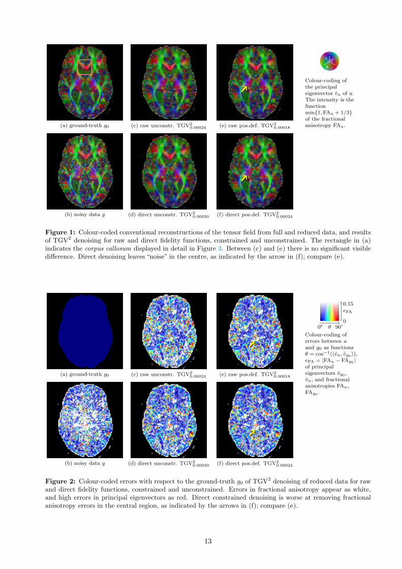
Raw versus direct, constrained versus unconstrained In Figure 1 we display the colour-codedresults for TGV2 with and without the positivity constraint for both the raw and direct fidelityfunctions. Figure 2 includes the corresponding colour-coded error plot, and Figure 3 displays thecorpus callosum region in detail, with greyscale coding of the fractional anisotropy, superimposed bythe principal eigenvectors. The location of this region in the brain is indicated in Figure 1. Finally,Figure 4 contains a visualisation of the positivity of the tensors.

As we see, direct unconstrained denoising has clearly the worst results, greatly over-smoothed. Wenote from Figure 4, however, that most negative eigenvalues within the brain mask are removed evenby unconstrained denoising. The effect of the constraint therefore lies primarily elsewhere.

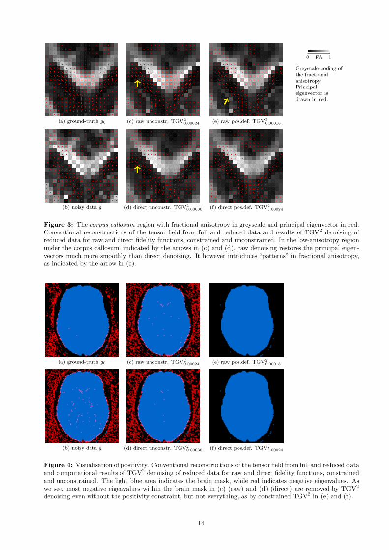
We see, moreover, that the constrained direct denoising result is very noisy in the central regionof the brain, while the raw denoising better restores the original data. The error plot of Figure2 indicates that direct denoising leaves more errors in fractional anisotropy in this area. Studyingthe corpus callosum in Figure 3, we see that direct denoising however better restores the dark (low-anisotropy) region under the high-anisotropy (near-white) corpus callosum. Raw DWI-based denoisinghowever has better performance with respect to the directions of the principal eigenvectors.

TGV2 versus TD, adding more noise The differences in the computational results in Table 1between TD and TGV2 are insignificant, and would be unobservable by the eye in the visualisations.We have therefore performed additional computations with a higher noise level. We still take s =(s0, s2, s4, s5, s6, s8, s11), and apply additional Rician noise of parameter σ = 10 to these signals. Wethen solve the tensor field g from (1.1).

10

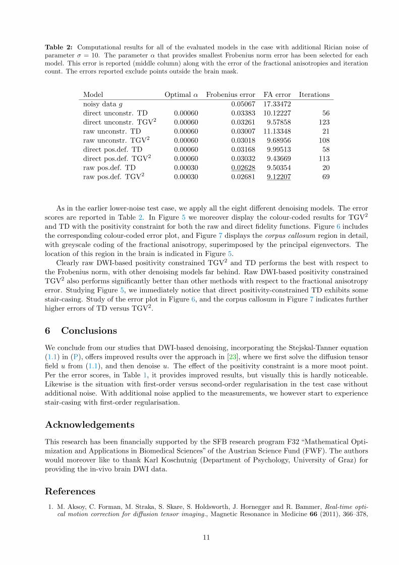
Table 2: Computational results for all of the evaluated models in the case with additional Rician noise ofparameter σ = 10. The parameter α that provides smallest Frobenius norm error has been selected for eachmodel. This error is reported (middle column) along with the error of the fractional anisotropies and iterationcount. The errors reported exclude points outside the brain mask.

Model Optimal α Frobenius error FA error Iterations

noisy data g 0.05067 17.33472direct unconstr. TD 0.00060 0.03383 10.12227 56direct unconstr. TGV2 0.00060 0.03261 9.57858 123raw unconstr. TD 0.00060 0.03007 11.13348 21raw unconstr. TGV2 0.00060 0.03018 9.68956 108direct pos.def. TD 0.00060 0.03168 9.99513 58direct pos.def. TGV2 0.00060 0.03032 9.43669 113raw pos.def. TD 0.00030 0.02628 9.50354 20raw pos.def. TGV2 0.00030 0.02681 9.12207 69

As in the earlier lower-noise test case, we apply all the eight different denoising models. The errorscores are reported in Table 2. In Figure 5 we moreover display the colour-coded results for TGV2

and TD with the positivity constraint for both the raw and direct fidelity functions. Figure 6 includesthe corresponding colour-coded error plot, and Figure 7 displays the corpus callosum region in detail,with greyscale coding of the fractional anisotropy, superimposed by the principal eigenvectors. Thelocation of this region in the brain is indicated in Figure 5.

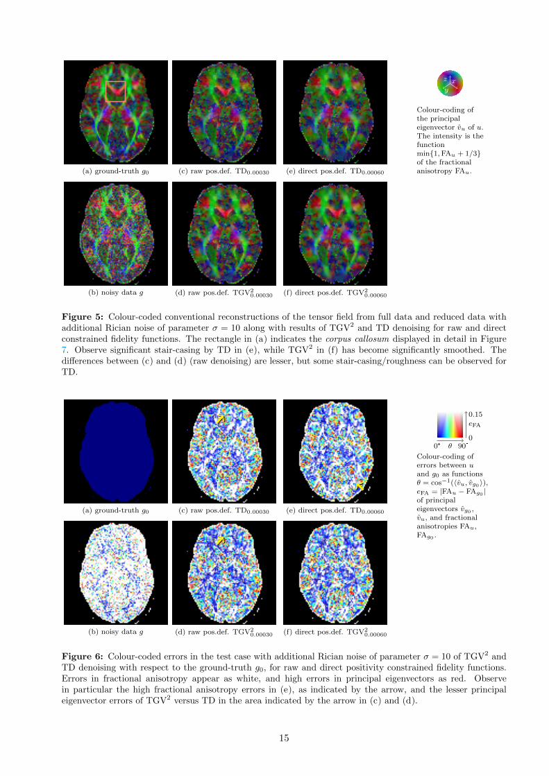
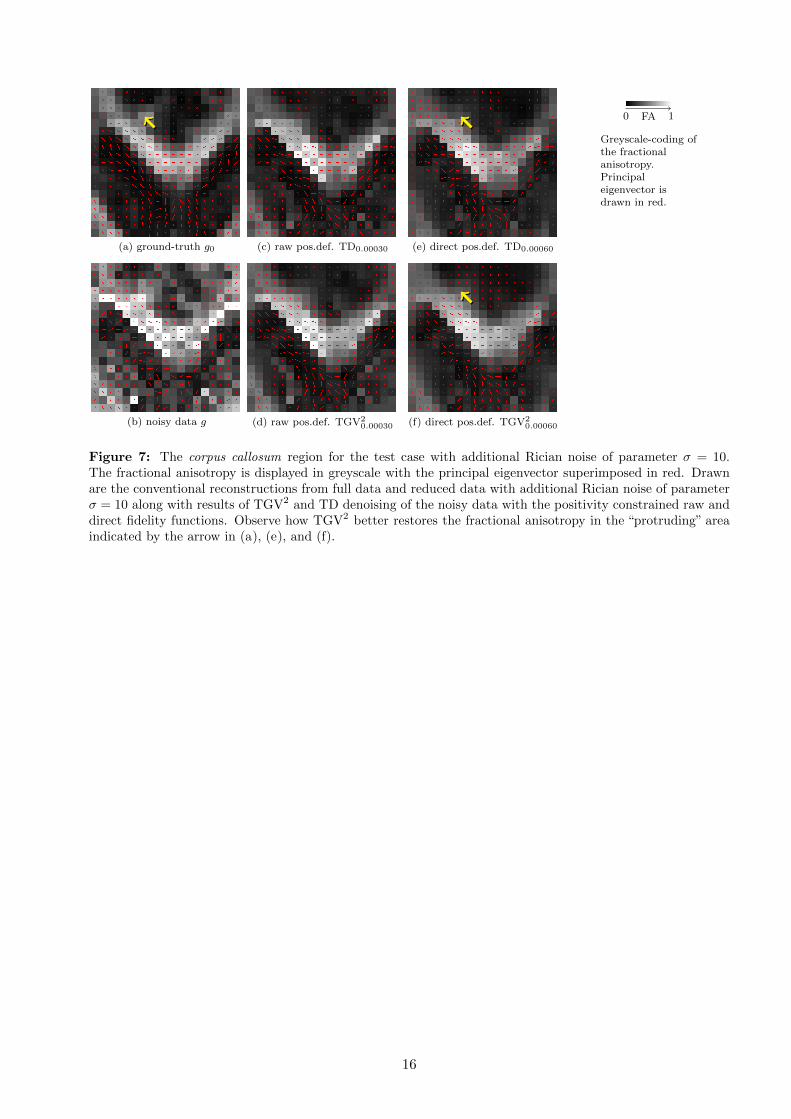
Clearly raw DWI-based positivity constrained TGV2 and TD performs the best with respect tothe Frobenius norm, with other denoising models far behind. Raw DWI-based positivity constrainedTGV2 also performs significantly better than other methods with respect to the fractional anisotropyerror. Studying Figure 5, we immediately notice that direct positivity-constrained TD exhibits somestair-casing. Study of the error plot in Figure 6, and the corpus callosum in Figure 7 indicates furtherhigher errors of TD versus TGV2.

6 Conclusions

We conclude from our studies that DWI-based denoising, incorporating the Stejskal-Tanner equation(1.1) in (P), offers improved results over the approach in [23], where we first solve the diffusion tensorfield u from (1.1), and then denoise u. The effect of the positivity constraint is a more moot point.Per the error scores, in Table 1, it provides improved results, but visually this is hardly noticeable.Likewise is the situation with first-order versus second-order regularisation in the test case withoutadditional noise. With additional noise applied to the measurements, we however start to experiencestair-casing with first-order regularisation.

Acknowledgements

This research has been financially supported by the SFB research program F32 “Mathematical Opti-mization and Applications in Biomedical Sciences” of the Austrian Science Fund (FWF). The authorswould moreover like to thank Karl Koschutnig (Department of Psychology, University of Graz) forproviding the in-vivo brain DWI data.

References

1. M. Aksoy, C. Forman, M. Straka, S. Skare, S. Holdsworth, J. Hornegger and R. Bammer, Real-time opti-cal motion correction for diffusion tensor imaging., Magnetic Resonance in Medicine 66 (2011), 366–378,

11

doi:10.1002/mrm.22787.

2. V. Arsigny, P. Fillard, X. Pennec and N. Ayache, Fast and simple computations on tensors with log-euclideanmetrics., Technical Report 5584, INRIA (2005).

3. P. J. Basser and D. K. Jones, Diffusion-tensor MRI: theory, experimental design and data analysis – atechnical review., NMR in Biomedicine 15 (2002), 456–467, doi:10.1002/nbm.783.

4. R. L. Bishop and S. I. Goldberg, Tensor Analysis on Manifolds, Dover Publications, 1980, Dover edition.

5. K. Bredies, Recovering piecewise smooth multichannel images by minimization of convex functionals withtotal generalized variation penalty, SFB-Report 2012-006, Karl-Franzens University of Graz (2012).

6. K. Bredies, K. Kunisch and T. Pock, Total generalized variation, SIAM J. Imaging Sci. 3 (2011), 492–526,doi:10.1137/090769521.

7. K. Bredies, K. Kunisch and T. Valkonen, Properties of L1-TGV2: The one-dimensional case, J. Math. AnalAppl. (2012). Accepted.

8. K. Bredies and T. Valkonen, Inverse problems with second-order total generalized variation constraints,in: Proceedings of SampTA 2011 – 9th International Conference on Sampling Theory and Applications,Singapore, 2011.

9. A. Chambolle and T. Pock, A first-order primal-dual algorithm for convex problems with applications toimaging, J. Math. Imaging Vision 40 (2011), 120–145, doi:10.1007/s10851-010-0251-1.

10. H. Federer, Geometric Measure Theory, Springer, 1969.

11. P. Fillard, X. Pennec, V. Arsigny and N. Ayache, Clinical DT-MRI estimation, smoothing, and fiber trackingwith log-Euclidean metrics, IEEE Trans. Medical Imaging 26 (2007), 1472–1482.

12. G. Golub and C. Van Loan, Matrix Computations, Johns Hopkins University Press, 1996.

13. H. Gudbjartsson and S. Patz, The Rician distribution of noisy MRI data, Magnetic Resonance in Medicine34 (1995), 910–914.

14. M. Herbst, J. Maclaren, M. Weigel, J. Korvink, J. Hennig and M. Zaitsev, Prospective motion correctionwith continuous gradient updates in diffusion weighted imaging, Magnetic Resonance in Medicine (2011),doi:10.1002/mrm.23230.

15. P. Kingsley, Introduction to diffusion tensor imaging mathematics: Parts I-III, Concepts in Magnetic Res-onance Part A 28 (2006), 101–179, doi:10.1002/cmr.a.20048. 10.1002/cmr.a.20049, 10.1002/cmr.a.20050.

16. F. Knoll, K. Bredies, T. Pock and R. Stollberger, Second order total generalized variation (TGV) for MRI.,Magnetic Resonance in Medicine 65 (2011), 480–491, doi:10.1002/mrm.22595.

17. R. T. Rockafellar and R. J.-B. Wets, Variational Analysis, Springer, 1998.

18. S. Setzer, G. Steidl, B. Popilka and B. Burgeth, Variational methods for denoising matrix fields, in: Visu-alization and Processing of Tensor Fields, Edited by J. Weickert and H. Hagen, Springer, 2009, 341–360.

19. S. M. Smith, M. Jenkinson, M. W. Woolrich, C. F. Beckmann, T. E. J. Behrens, H. Johansen-Berg, P. R.Bannister, M. D. Luca, I. Drobnjak, D. E. Flitney, R. K. Niazy, J. Saunders, J. Vickers, Y. Zhang, N. D.Stefano, J. M. Brady and P. M. Matthews, Advances in functional and structural MR image analysis and im-plementation as FSL., Neuroimage 23 Suppl 1 (2004), S208–S219, doi:10.1016/j.neuroimage.2004.07.051.

20. R. Temam, Mathematical problems in plasticity, Gauthier-Villars, 1985.

21. J.-D. Tournier, S. Mori and A. Leemans, Diffusion tensor imaging and beyond, Magnetic Resonance inMedicine 65 (2011), 1532–1556, doi:10.1002/mrm.22924.

22. T. Valkonen, A method for weighted projections to the positive definite cone, SFB-Report 2012-016, Karl-Franzens University of Graz (2012).

23. T. Valkonen and F. Knoll, Total generalised variation in diffusion tensor imaging, SFB-Report 2012-003,Karl-Franzens University of Graz (2012).

12

(a) ground-truth g0 (c) raw unconstr. TGV20.00024 (e) raw pos.def. TGV2

0.00018

(b) noisy data g (d) direct unconstr. TGV20.00030 (f) direct pos.def. TGV2

0.00024

xy

z

Colour-coding ofthe principaleigenvector vu of u.The intensity is thefunctionmin1,FAu + 1/3of the fractionalanisotropy FAu.

Figure 1: Colour-coded conventional reconstructions of the tensor field from full and reduced data, and resultsof TGV2 denoising for raw and direct fidelity functions, constrained and unconstrained. The rectangle in (a)indicates the corpus callosum displayed in detail in Figure 3. Between (c) and (e) there is no significant visibledifference. Direct denoising leaves “noise” in the centre, as indicated by the arrow in (f); compare (e).

(a) ground-truth g0 (c) raw unconstr. TGV20.00024 (e) raw pos.def. TGV2

0.00018

(b) noisy data g (d) direct unconstr. TGV20.00030 (f) direct pos.def. TGV2

0.00024

0

eFA

0.15

0° θ 90°

Colour-coding oferrors between uand g0 as functionsθ = cos−1(〈vu, vg0 〉),eFA = |FAu − FAg0 |of principaleigenvectors vg0 ,vu, and fractionalanisotropies FAu,FAg0 .

Figure 2: Colour-coded errors with respect to the ground-truth g0 of TGV2 denoising of reduced data for rawand direct fidelity functions, constrained and unconstrained. Errors in fractional anisotropy appear as white,and high errors in principal eigenvectors as red. Direct constrained denoising is worse at removing fractionalanisotropy errors in the central region, as indicated by the arrows in (f); compare (e).

13

(a) ground-truth g0 (c) raw unconstr. TGV20.00024 (e) raw pos.def. TGV2

0.00018

(b) noisy data g (d) direct unconstr. TGV20.00030 (f) direct pos.def. TGV2

0.00024

0 FA 1

Greyscale-coding ofthe fractionalanisotropy.Principaleigenvector isdrawn in red.

Figure 3: The corpus callosum region with fractional anisotropy in greyscale and principal eigenvector in red.Conventional reconstructions of the tensor field from full and reduced data and results of TGV2 denoising ofreduced data for raw and direct fidelity functions, constrained and unconstrained. In the low-anisotropy regionunder the corpus callosum, indicated by the arrows in (c) and (d), raw denoising restores the principal eigen-vectors much more smoothly than direct denoising. It however introduces “patterns” in fractional anisotropy,as indicated by the arrow in (e).

(a) ground-truth g0 (c) raw unconstr. TGV20.00024 (e) raw pos.def. TGV2

0.00018

(b) noisy data g (d) direct unconstr. TGV20.00030 (f) direct pos.def. TGV2

0.00024

Figure 4: Visualisation of positivity. Conventional reconstructions of the tensor field from full and reduced dataand computational results of TGV2 denoising of reduced data for raw and direct fidelity functions, constrainedand unconstrained. The light blue area indicates the brain mask, while red indicates negative eigenvalues. Aswe see, most negative eigenvalues within the brain mask in (c) (raw) and (d) (direct) are removed by TGV2

denoising even without the positivity constraint, but not everything, as by constrained TGV2 in (e) and (f).

14

(a) ground-truth g0 (c) raw pos.def. TD0.00030 (e) direct pos.def. TD0.00060

(b) noisy data g (d) raw pos.def. TGV20.00030 (f) direct pos.def. TGV2

0.00060

xy

z

Colour-coding ofthe principaleigenvector vu of u.The intensity is thefunctionmin1,FAu + 1/3of the fractionalanisotropy FAu.

Figure 5: Colour-coded conventional reconstructions of the tensor field from full data and reduced data withadditional Rician noise of parameter σ = 10 along with results of TGV2 and TD denoising for raw and directconstrained fidelity functions. The rectangle in (a) indicates the corpus callosum displayed in detail in Figure7. Observe significant stair-casing by TD in (e), while TGV2 in (f) has become significantly smoothed. Thedifferences between (c) and (d) (raw denoising) are lesser, but some stair-casing/roughness can be observed forTD.

(a) ground-truth g0 (c) raw pos.def. TD0.00030 (e) direct pos.def. TD0.00060

(b) noisy data g (d) raw pos.def. TGV20.00030 (f) direct pos.def. TGV2

0.00060

0

eFA

0.15

0° θ 90°

Colour-coding oferrors between uand g0 as functionsθ = cos−1(〈vu, vg0 〉),eFA = |FAu − FAg0 |of principaleigenvectors vg0 ,vu, and fractionalanisotropies FAu,FAg0 .

Figure 6: Colour-coded errors in the test case with additional Rician noise of parameter σ = 10 of TGV2 andTD denoising with respect to the ground-truth g0, for raw and direct positivity constrained fidelity functions.Errors in fractional anisotropy appear as white, and high errors in principal eigenvectors as red. Observein particular the high fractional anisotropy errors in (e), as indicated by the arrow, and the lesser principaleigenvector errors of TGV2 versus TD in the area indicated by the arrow in (c) and (d).

15

(a) ground-truth g0 (c) raw pos.def. TD0.00030 (e) direct pos.def. TD0.00060

(b) noisy data g (d) raw pos.def. TGV20.00030 (f) direct pos.def. TGV2

0.00060

0 FA 1

Greyscale-coding ofthe fractionalanisotropy.Principaleigenvector isdrawn in red.

Figure 7: The corpus callosum region for the test case with additional Rician noise of parameter σ = 10.The fractional anisotropy is displayed in greyscale with the principal eigenvector superimposed in red. Drawnare the conventional reconstructions from full data and reduced data with additional Rician noise of parameterσ = 10 along with results of TGV2 and TD denoising of the noisy data with the positivity constrained raw anddirect fidelity functions. Observe how TGV2 better restores the fractional anisotropy in the “protruding” areaindicated by the arrow in (a), (e), and (f).

16