the constrained interpolation profile method for multiphase analysis
TRANSCRIPT
Journal of Computational Physics169,556–593 (2001)
doi:10.1006/jcph.2000.6625, available online at http://www.idealibrary.com on
The Constrained Interpolation Profile Methodfor Multiphase Analysis
Takashi Yabe,∗ Feng Xiao,∗,† and Takayuki Utsumi†,‡∗Department of Mechanical Engineering and Science, Tokyo Institute of Technology, O-okayama, Meguro-ku,
Tokyo 152-8552, Japan;‡Advanced Photon Research Center, Kansai Research Establishment, JapanAtomic Energy Research Institute, 25-1 Miiminami-machi, Neyagawa, Osaka 572-0019, Japan;
and†Frontier Research System for Global Change, SEAVANS North, 1-2-1 Shibaura,Minato-ku, Tokyo 105-6791, Japan
Received December 16, 1999; revised August 3, 2000
We present a review of the constrained interpolation profile (CIP) method that isknown as a general numerical solver for solid, liquid, gas, and plasmas. This methodis a kind of semi-Lagrangian scheme and has been extended to treat incompressibleflow in the framework of compressible fluid. Since it uses primitive Euler repre-sentation, it is suitable for multiphase analysis. The recent version of this methodguarantees the exact mass conservation even in the framework of a semi-Lagrangianscheme. We provide a comprehensive review of the strategy of the CIP method, whichhas a compact support and subcell resolution, including a front-capturing algorithmwith functional transformation, a pressure-based algorithm, and other miscellaneousphysics such as the elastic–plastic effect and surface tension. Some practical appli-cations are also reviewed, such as milk crown or coronet, laser-induced melting, andturbulent mixing layer of liquid–gas interface. c© 2001 Academic Press
Key Words:numerical algorithm; semi-Lagrangian schemes; interface capturing;fluid dynamics; mass conservation; multiphase flows; surface tension; rheologicalmaterials.
1. INTRODUCTION
Recent high technology requires new tools for combined analysis of materials in differentphase states, e.g., solid, liquid, and gas. A universal treatment of all phases by one simplealgorithm would be useful and we are at the point of attacking this goal. For these typesof problems, for example, welding and cutting processes, we need to treat topology andphase changes of the structure simultaneously, where the grid system aligned to the solidor liquid surface has no meaning and sometimes the mesh is distorted and even broken up.To solve these problems with Lagrangian representation in finite-difference, finite-element,and boundary-element methods will be a challenging task.
556
0021-9991/01 $35.00Copyright c© 2001 by Academic PressAll rights of reproduction in any form reserved.

CIP METHOD FOR MULTIPHASE ANALYSIS 557
Even without phase change, solving the problem of structure–fluid interaction is not aneasy task. In most cases, the grid cannot always be adapted to the solid surface. Therefore,the description of moving solid surfaces of complicated shapes in the Cartesian grid systemis a challenging subject [57].
To attack the problems mentioned above, we must first find a method to treat a sharpinterface and to solve the interaction of compressible gas with incompressible liquid or solid.For compressible fluid, elaborate schemes like TVD (total variation diminishing) or ENO(essentially nonoscillating) proved to be effective in capturing shock waves. However, sincethese schemes employ a conservative form of fluid equations, divergence of velocity whichbecomes zero in the incompressible limit cannot be treated independent of the advectionpart. Furthermore, as Karni [15] pointed out, the conservative algorithm sometimes givesfictitious pressure undulation at the boundary of multiphase materials.
On the other hand, incompressible schemes like QUICK or higher-order upwind schemescan treat divergence-free fluid vorticity and turbulence. However, these schemes cannotalways treat a shock wave as a sharp discontinuity.
We need a scheme for treating both compressible and incompressible fluids with largedensity ratios simultaneously in one program to simulate the interaction of gas with aliquid or solid. Fully implicit solvers can handle this procedure, but the convergence ofiteration in a highly distorted state is still a problem. Toward this goal, we take a Eu-lerian approach based on the CIP (cubic-interpolated propagation) method [40, 41, 60–62] which does not need an adaptive grid system and therefore eliminates the problemsof grid distortion caused by structural breakup and topology change. The material sur-face can almost be captured by one grid throughout the computation [64, 65]. Further-more, the code can treat all the phases of matter from solid state through liquid andfrom two-phase state to gas without restriction on the time step from high-sound speed[63].
A pressure-based algorithm coupled with a semi-Lagrangian approach such as the CIPproved to be stable and robust in analyzing these subjects. One disadvantage of this methodwas the lack of conservative property. Recent versions of the CIP-CSL4 (conservativesemi-Lagrangian) [43] can overcome this difficulty and provide exactly a conservative semi-Lagrangian scheme. Since these schemes do not use cubic polynomials but rather differentorders of polynomials, we have renamed these CIP families “constrained interpolationprofile” and kept the abbreviation CIP. This means that various constraints such as thetime evolution of a spatial gradient, which is used in the original CIP method, or spatiallyintegrated conservative quantities can be used to construct the profile. In this paper, wereview the CIP method and related schemes and address these important subjects.
In Section 2, the CIP method is derived for advection calculation. After a descriptionof the fundamental idea of the method with a 1D problem, some variants and practi-cal extensions are discussed. They include, for example, multidimensional formulation,oscillation-suppressing interpolation, and sharpness enhancement. A formulation of theCIP method applied to general hydrodynamics is presented in Section 3. Section 4 dis-cusses a unified procedure to compute both compressible and incompressible fluids withseveral examples. Some numerical formulations for interfacial flows, including surface ten-sion and the elastic–plastic effect, are presented in Section 5. As a recent improvement to theCIP method, conservative variants of the method are briefly discussed with a few numericalexamples. The paper ends with a short summary referencing some applications in otherfields.
558 YABE, XIAO, AND UTSUMI
2. THE ADVECTION PROCESS
2.1. CIP Formulation in One Dimension
Although nature operates in a continuous world, a discretization process is unavoidablefor implementing numerical simulations. The primary goal of any numerical algorithm willbe to retrieve the information lost inside the grid cell between these digitized points. TheCIP method proposed by one of the authors tries to construct a solution inside the grid cellthat is close enough to the real solution of the given equation, with some constraints. Wehere explain the strategy of the CIP method by using an advection equation,
∂ f
∂t+ u
∂ f
∂x= 0. (1)
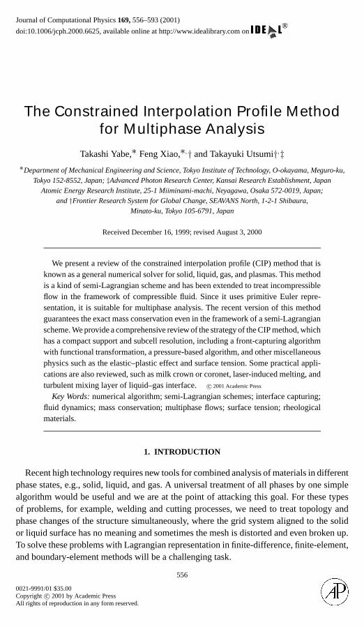
When the velocity is constant, the solution of Eq. (1) gives a simple translational motion ofa wave with velocityu. The initial profile (the solid line in Fig. 1a) moves like a dashed linein a continuous representation. At this time, the solution at grid points is denoted by circlesand is the same as the exact solution. However, if we eliminate the dashed line as in Fig. 1b,then the information about the profile inside the grid cell has been lost, and it is difficultto imagine the original profile and natural to imagine a profile such as that shown by thesolid line in (c). Thus, numerical diffusion arises when we construct the profile by the linearinterpolation, even with the exact solution shown in Fig. 1c. This process is called the first-order upwind scheme. On the other hand, if we use a quadratic polynomial for interpolation,the model suffers from overshooting. This process is called the Lax–Wendroff scheme orthe Leith scheme [18].
What made this solution worse? This decline in accuracy is the reason we neglect thebehavior of the solution inside the grid cell and merely follow the smoothness of the solution.From this consideration, we can see that it is important to develop a method incorporatingthe real solution into the profile within a grid cell. We propose an approximation of theprofile as shown below. If we differentiate Eq. (1) with spatial variablex, we get
∂g
∂t+ u
∂g
∂x= −∂u
∂xg, (2)
FIG. 1. The principle of the CIP method. (a) The solid line is the initial profile and the dashed line is anexact solution after advection, shown in (b) at discretized points. (c) When (b) is linearly interpolated, numericaldiffusion appears. (d) In the CIP, the spatial derivative also propagates and the profile inside a grid cell is retrieved.
CIP METHOD FOR MULTIPHASE ANALYSIS 559
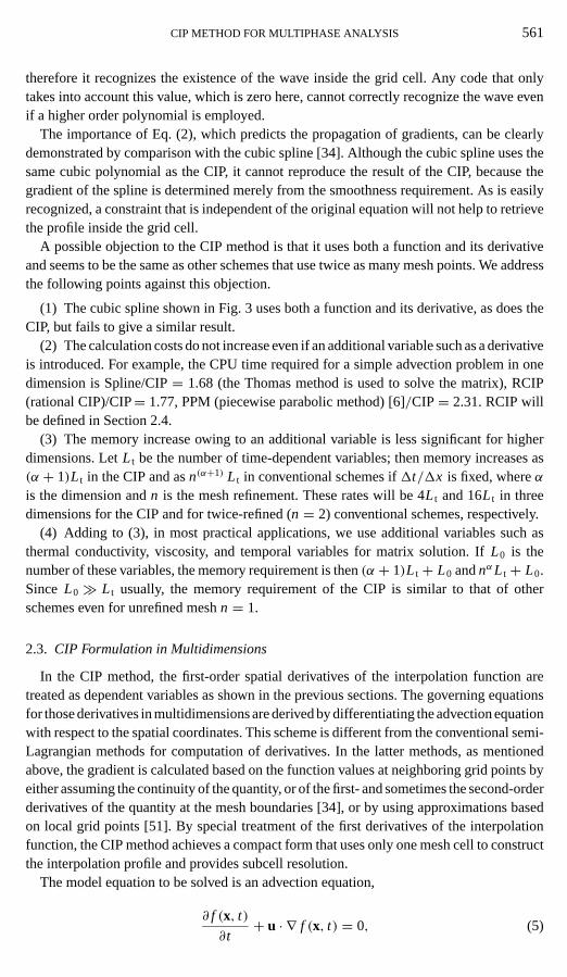
where g stands for the spatial derivative off , ∂ f/∂x. In the simplest case where thevelocity u is constant, Eq. (2) coincides with Eq. (1) and represents the propagation of aspatial derivative with velocityu. Using this equation, we can trace the time evolution off andg on the basis of Eq. (1). Ifg is predicted after propagation as shown by the arrowsin Fig. 1d, the profile after one step is limited to a specific profile. It is easy to imaginethat by this constraint, the solution becomes much closer to the initial profile that is thereal solution. Most importantly, the solution thus created gives a profile consistent withEq. (1) even inside the grid cell. The importance of this constraint is demonstrated in thenext section.
If two values of f andg are given at two grid points, the profile between these points canbe interpolated by the cubic polynomialF(x) = ax3+ bx2+ cx+ d. Thus, the profile atthen+ 1 step can be obtained by shifting the profile byu1t so that
f n+1 = F(x − u1t),
gn+1 = d F(x − u1t)/dx.(3)
ai = gi + giup
D2+ 2( fi − fiup)
D3,
bi = 3( fiup− fi )
D2− 2gi + giup
D,
f n+1i = ai ξ
3+ bi ξ2+ gn
i ξ + f ni ,
(4)gn+1
i = 3ai ξ2+ 2bi ξ + gn
i ,
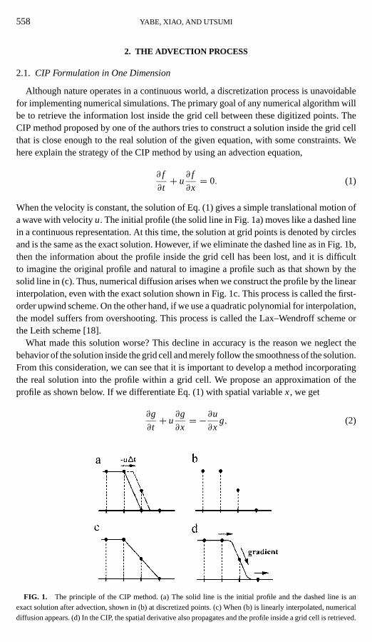
where we defineξ = −u1t . Here,D = −1x, iup= i − 1 for u ≥ 0 andD = 1x, iup=i + 1 for u < 0. Figure 2a shows a profile after 1000 steps with this CIP method for thepropagation of a square wave.
The CIP advection scheme can be sorted out as a kind of semi-Lagrangian method inthe sense that the CIP advection scheme employs a Lagrangian invariant solution. Semi-Lagrangian methods that trace back along the characteristics in time depend on an interpo-lation of the initial profile to determine the value at the upstream departure point (whichmay not coincide with the computational grid point).
Although there are various polynomial functions such as linear, quadratic Lagrange,cubic Lagrange, cubic spline, and quintic Lagrange [37], all of these schemes (exceptthose using the linear interpolation function) need at least three points for constructinginterpolation approximations in one dimension. A more compact scheme by which one
FIG. 2. (a) Initial condition, and the profile after one complete revolution with (b) CIP, and (c) rational CIPand tangent-transformed CIP.

560 YABE, XIAO, AND UTSUMI
FIG. 3. Phase error of various schemes such as first-order upwind, Lax–Wendroff (LW), PPM, Spline, andCIP.
can construct interpolation functions of high accuracy with fewer computational stencils isdesired in many situations, such as calculating discontinuities or large gradients. A schemethat is based on a compact support is able to localize dispersion errors to the regionswhere large local gradients appear. Moreover, in a model with a limited computationaldomain, different approximations for the derivatives must be used at the grid points closeto boundaries; these approximations are usually of lower order than the approximationsused deeper in the interior. Thus, a scheme that uses fewer stencils may be advantageous intreating computational boundaries since fewer boundary points need to be handled. Anotherattractive feature of reducing the number of stencils may be the reduction in data transfer inparallel implementations on distributed memory architectures. In this sense, the CIP seemsto be attractive since it uses only one cell for computation even in three dimensions.
2.2. Mathematical Analysis of CIP
It is interesting to examine the phase error of various schemes using the method proposedby Purnell [34] and Utsumiet al.[46]. Figure 3 summarizes those results. As is well known,phase speeds in conventional schemes depart from the exact speed, shown by the solid line,which is aroundk1x = π/2. Surprisingly, however, the CIP can reproduce the correctphase speed even up tok1x = π . This is remarkable becausek1x = π means that onewavelength is described by three mesh points. Let us consider the case shown in Fig. 4,where values of the three points are zero. Even in this case, one wave can exist as shownin Fig. 4. The CIP gives correct spatial gradients, which are non-zero at these points, and
FIG. 4. The CIP can correctly recognize one wavelength with three grid points.
CIP METHOD FOR MULTIPHASE ANALYSIS 561
therefore it recognizes the existence of the wave inside the grid cell. Any code that onlytakes into account this value, which is zero here, cannot correctly recognize the wave evenif a higher order polynomial is employed.
The importance of Eq. (2), which predicts the propagation of gradients, can be clearlydemonstrated by comparison with the cubic spline [34]. Although the cubic spline uses thesame cubic polynomial as the CIP, it cannot reproduce the result of the CIP, because thegradient of the spline is determined merely from the smoothness requirement. As is easilyrecognized, a constraint that is independent of the original equation will not help to retrievethe profile inside the grid cell.
A possible objection to the CIP method is that it uses both a function and its derivativeand seems to be the same as other schemes that use twice as many mesh points. We addressthe following points against this objection.
(1) The cubic spline shown in Fig. 3 uses both a function and its derivative, as does theCIP, but fails to give a similar result.
(2) The calculation costs do not increase even if an additional variable such as a derivativeis introduced. For example, the CPU time required for a simple advection problem in onedimension is Spline/CIP= 1.68 (the Thomas method is used to solve the matrix), RCIP(rational CIP)/CIP= 1.77, PPM (piecewise parabolic method) [6]/CIP= 2.31. RCIP willbe defined in Section 2.4.
(3) The memory increase owing to an additional variable is less significant for higherdimensions. LetL t be the number of time-dependent variables; then memory increases as(α + 1)L t in the CIP and asn(α+1) L t in conventional schemes if1t/1x is fixed, whereαis the dimension andn is the mesh refinement. These rates will be 4L t and 16L t in threedimensions for the CIP and for twice-refined (n = 2) conventional schemes, respectively.
(4) Adding to (3), in most practical applications, we use additional variables such asthermal conductivity, viscosity, and temporal variables for matrix solution. IfL0 is thenumber of these variables, the memory requirement is then(α + 1)L t + L0 andnαL t + L0.Since L0À L t usually, the memory requirement of the CIP is similar to that of otherschemes even for unrefined meshn = 1.
2.3. CIP Formulation in Multidimensions
In the CIP method, the first-order spatial derivatives of the interpolation function aretreated as dependent variables as shown in the previous sections. The governing equationsfor those derivatives in multidimensions are derived by differentiating the advection equationwith respect to the spatial coordinates. This scheme is different from the conventional semi-Lagrangian methods for computation of derivatives. In the latter methods, as mentionedabove, the gradient is calculated based on the function values at neighboring grid points byeither assuming the continuity of the quantity, or of the first- and sometimes the second-orderderivatives of the quantity at the mesh boundaries [34], or by using approximations basedon local grid points [51]. By special treatment of the first derivatives of the interpolationfunction, the CIP method achieves a compact form that uses only one mesh cell to constructthe interpolation profile and provides subcell resolution.
The model equation to be solved is an advection equation,
∂ f (x, t)∂t
+ u · ∇ f (x, t) = 0, (5)
562 YABE, XIAO, AND UTSUMI
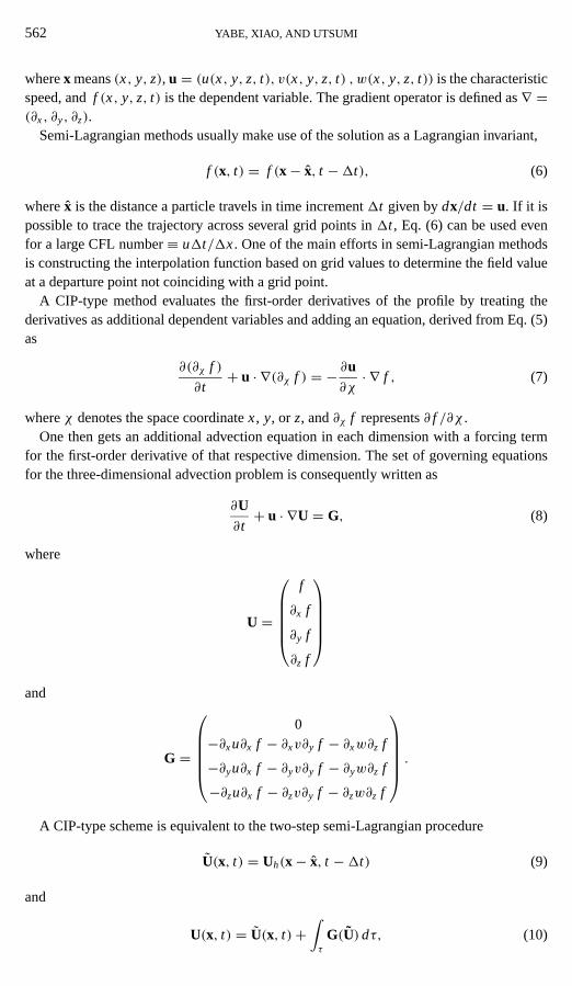
wherex means(x, y, z), u = (u(x, y, z, t), v(x, y, z, t) , w(x, y, z, t)) is the characteristicspeed, andf (x, y, z, t) is the dependent variable. The gradient operator is defined as∇ =(∂x, ∂y, ∂z).
Semi-Lagrangian methods usually make use of the solution as a Lagrangian invariant,
f (x, t) = f (x− x, t −1t), (6)
wherex is the distance a particle travels in time increment1t given bydx/dt = u. If it ispossible to trace the trajectory across several grid points in1t , Eq. (6) can be used evenfor a large CFL number≡ u1t/1x. One of the main efforts in semi-Lagrangian methodsis constructing the interpolation function based on grid values to determine the field valueat a departure point not coinciding with a grid point.
A CIP-type method evaluates the first-order derivatives of the profile by treating thederivatives as additional dependent variables and adding an equation, derived from Eq. (5)as
∂(∂χ f )
∂t+ u · ∇(∂χ f ) = − ∂u
∂χ· ∇ f , (7)
whereχ denotes the space coordinatex, y, or z, and∂χ f represents∂ f /∂χ .One then gets an additional advection equation in each dimension with a forcing term
for the first-order derivative of that respective dimension. The set of governing equationsfor the three-dimensional advection problem is consequently written as
∂U∂t+ u · ∇U = G, (8)
where
U =
f
∂x f
∂y f
∂z f
and
G =
0
−∂xu∂x f − ∂xv∂y f − ∂xw∂z f
−∂yu∂x f − ∂yv∂y f − ∂yw∂z f
−∂zu∂x f − ∂zv∂y f − ∂zw∂z f
.A CIP-type scheme is equivalent to the two-step semi-Lagrangian procedure
U(x, t) = Uh(x− x, t −1t) (9)
and
U(x, t) = U(x, t)+∫τ
G(U) dτ, (10)
CIP METHOD FOR MULTIPHASE ANALYSIS 563
whereUh represents the interpolation approximation toU, andτ denotes the trajectory thatconnects(x, t −1t) and(x, t).
Once the interpolation function is determined from the continuity condition imposed onthe dependent variable and its first-order derivatives at the grid points, we immediately getthe solution to the advection equation from Eqs. (9) and (10).
Several forms of the multidimensional cubic polynomial have been proposed [2, 62].Among various families of polynomial, the simplest one is written as [62]
Fi, j (x, y) = C3,0X3+ C2,0X2+ fxi, j X + fi, j + C0,3Y3+ C0,2Y2+ fyi, j Y
+C2,1X2Y + C1,1XY+ C1,2XY2, (11)
which has a form consistent with one-dimensional CIP in one direction. Here we defineX = x − xi , Y = y− yj . Thus 10 unknowns are determined from the continuity off ;∂ f/∂x; ∂ f/∂y at (i , j ), (i + 1, j ), (i , j + 1); and the continuity off at (i + 1, j + 1).
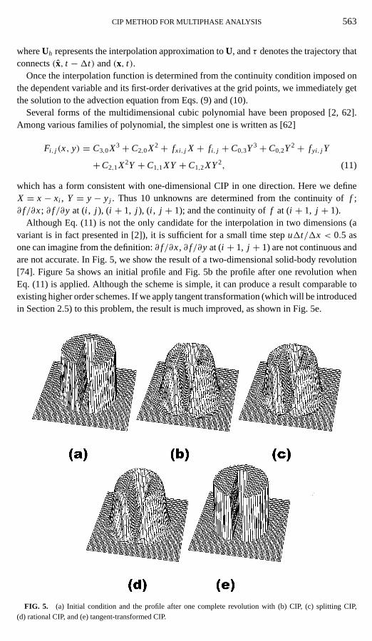
Although Eq. (11) is not the only candidate for the interpolation in two dimensions (avariant is in fact presented in [2]), it is sufficient for a small time stepu1t/1x < 0.5 asone can imagine from the definition:∂ f/∂x, ∂ f/∂y at (i + 1, j + 1) are not continuous andare not accurate. In Fig. 5, we show the result of a two-dimensional solid-body revolution[74]. Figure 5a shows an initial profile and Fig. 5b the profile after one revolution whenEq. (11) is applied. Although the scheme is simple, it can produce a result comparable toexisting higher order schemes. If we apply tangent transformation (which will be introducedin Section 2.5) to this problem, the result is much improved, as shown in Fig. 5e.
FIG. 5. (a) Initial condition and the profile after one complete revolution with (b) CIP, (c) splitting CIP,(d) rational CIP, and (e) tangent-transformed CIP.

564 YABE, XIAO, AND UTSUMI
In these cases, the multidimensional profile is shifted in the direction of velocity vectoru. In addition, a directional splitting technique can be used to perform sequential one-dimensional advection in each direction. The latter method is very promising because itwould be difficult to construct a cubic polynominal in six-dimensional hyperspace suchas the Vlasov equation, and a conservative scheme can be readily constructed using thissplitting scheme [21]. Figure 5, which includes the result of this scheme, shows that thesymmetry of the profile is preserved well.
2.4. The RCIP Scheme for the Advection Equation
In practical implementation, an attractive advection scheme should be both low in dif-fusion and free of oscillation. In modern Eulerian high-resolution schemes, manipulationssuch as numerical viscosity are usually done to degrade the scheme to a lower order inthe presence of discontinuities in order to eliminate spurious oscillation. Some of theseschemes are reviewed by Toro [44]. Preserving the shape of the advected field is also one ofthe primary goals for semi-Lagrangian schemes, since a scheme with an interpolator higherthan second order will produce spurious oscillations near large gradients or discontinuities.Williamson and Rasch [51] discuss several shape-preserving interpolation schemes. Themonotonicity of a scheme is improved by imposing derivative constraints on a Hermitecubic or a rational-cubic interpolation function. Bermejo and Staniforth [4] also reportedtheir work on overcoming the numerical oscillation for semi-Lagrangian schemes, wherea minimum/maximum limiter is imposed on the calculated results from any conventionalsemi-Lagrangian scheme, based on the argument that no new extremum should be createdby an advection scheme.
The original CIP method, which uses a cubic polynomial interpolant, produces numericaloscillations near the area where the dependent variable has a degree of smoothness no morethan 1, which is onlyC0 for a step or a triangle distribution. A numerical scheme to get ashape-preserving scheme for a CIP-type method was developed from a rational interpolationfunction over one mesh cell [54, 55]. This scheme, which we call the RCIP (rational-cubicinterpolation propagation) scheme, shows good properties in keeping the topological natureof data, such as preserving convexity or concavity.
The 1D scheme is based on the rational function
R1Di (x) =
∑0≤l x≤3
∑0≤p≤1
αpβpX p
−1
Clx Xlx , (12)
whereX = x − xi and
C0 = fi
C1 = gi + fiα1β1
C2 = Siα1β1+ (Si − di )1i−1− C31i
C3 = [gi − Si + (giup− Si )(1+ α1β11i )]1i−2
α0 = 1.0
β0 = 1.0
β1 = [|(Si − gi )/(giup− Si )| − 1]1i−1;
CIP METHOD FOR MULTIPHASE ANALYSIS 565
here 1i = xiup− xi
Si = ( fiup− fi )1i−1
gi = (d f/dx)i .
In deriving the above coefficients, we first determinedβ1 by settingC3 = 0, which meansa second-order polynomial is the numerator of Eq. (12) becauseβ1 should be effective at thediscontinuity where the scheme becomes lower order. Therefore four constraints fromf andg at neighboring points are sufficient to determine these coefficients. After determiningβ1,we use it as a fixed value and then recoverC3 and uniquely determine the cubic polynomialby the same four constraints [55].
Then a solution to the advection equation can be written as
f n+1i = R1D
i (xi − u1t) = C0+ C1ξ + C2ξ2+ C3ξ
3
1+ α1β1ξ, (13)
and the first-order derivative of the dependent variable is calculated by
gn+1i = ∂x f n+1
i = ∂x R1Di (xi − u1t) = (C1+ 2C2ξ + 3C3ξ
2)(1+ α1β1ξ)−1
−α1β1(C0+ C1ξ + C2ξ2+ C3ξ
3)(1+ α1β1ξ)−2−
(∂u
∂x
∂ f
∂x
)n
i
, (14)
whereξ = −u1t . All the coefficients in the above expressions can be computed from thequantities off andg at stepn. It is interesting to see that the second term on the right-handside of Eq. (14) is proportional to−α1β1 and hence plays a role in reducing the contributionfrom the highest order polynomial, theα1β1C3ξ
3 term, tog at the discontinuity.The parameterα1 ∈ [0, 1] provides flexibility to choose between a rational function and
a cubic function for interpolation. In practical computations, we recommend the followingswitching formulation to put the interpolatant “cubic” in the smooth region and the “rational”near discontinuity:
α1 =
1, gi · giup < 0;0, gi · giup ≥ 0.
(15)
The subscriptiup indicates an upwind grid point. The smoothness is detected by seeingwhether the first-order derivative, which is computed as a dependent variable in the CIPmethod, has the same sign at neighboring grid points. When the switching parameterα1 isset to zero, algorithm (13), (14) is identical to the original CIP method. Letα1 = 1; under theCFL condition, scheme (13), (14) is convex–concave preserving and monotone preservingif the given data are nonconcave or nonconvex, as proved in Ref. [54].
Numerical experiments, shown in Fig. 2b demonstrate that the scheme of Eqs. (13) and(14) is capable of suppressing the spurious oscillation near discontinuities.
Fully two- and three-dimensional schemes can also be constructed by making use of thefollowing interpolation functions (see [55] for details).
R2Di, j (x, y) =
∑0≤p+q≤1
αp,qβp,q X pYq
−1 ∑0≤l x+l y≤3
Clx,l y Xlx Yl y, (16)
566 YABE, XIAO, AND UTSUMI
and
R3Di, j,k(x, y, z) =
∑0≤p+q+r≤1
αp,q,rβp,q,r X pYq Zr
−1 ∑0≤l x+l y+l z≤3
Clx,l y,l z Xlx Yl y Zlz. (17)
Figure 5 includes the test run with this RCIP scheme.
2.5. Interface Tracking: A Sharpness-Preserving Method
Treatment of the interface that lies between materials of different properties remains aformidable challenge to the computation of multiphase fluid dynamics. Eulerian methodshave proven robust in simulating flows with interfaces of complex topology. Generally,Eulerian methods use color function to distinguish among regions containing differentmaterials. To accurately reproduce the physical processes that occur across the interfacetransition region, maintaining the compact thickness of the interface is very important. Thefinite-difference schemes constructed on a Eulerian grid, however, intrinsically producenumerical diffusions to the solution of the advection equation by which the interface ispredicted temporally. Thus, the direct implementation of finite-difference schemes (eventhose of high order) cannot maintain the compactness of the interface.
Various kinds of methods have been developed to achieve a compact and correctly definedinterface by introducing extra programming. Among the most common algorithms are thelevel-set methods and the VOF (volume-of-fluid) methods for front capturing, and othersfor front tracking [45]. The level set method that was first proposed by Osheret al. [24,29, 38] gets around the computation of interfacial discontinuity by evaluating the field inhigher dimensions. The interface of interest is then recovered by taking a subset of thefield. Practically, the interface is defined as the zero-level set of a distance function fromthe interface.
In VOF methods, on the other hand, the interface needs to be reconstructed based on thevolume fraction of fluid. VOF methods are mainly classified as SLIC (simple line inter-face calculation) algorithms and PLIC (piecewise linear interface calculation) algorithmsaccording to the interpolation function used to represent the interface. The SLIC [11] algo-rithm makes use of piecewise constant reconstruction, and the interfaces are approximatedby lines aligned with mesh coordinates. A significant improvement in the VOF methodwas made by Youngs with the PLIC algorithm [71]. Since then, some improvements in thereconstruction of the VOF interface have been reported [16, 32, 33]. The PLIC algorithmestimates the interface with a truly piecewise linear approximation that greatly improvesthe geometrical faithfulness of the method. A comparison of various methods for trackinginterfaces can be found in [35].
In [64] and [65], we devised an interface tracking technique that appears to be efficient,geometrically faithful, and diffusionless. The method is a combination of the CIP advectionsolver and a tangent function transformation.
ConsiderK kinds of impermeable materials occupying closed areasÄk(t), k = 1, 2, . . . ,K in computational domainD ∈ R3(x, y, z). We identify them with color functions or den-sity functionsφk(x, y, z, t), k = 1, 2, . . . , K according to the following definition.
φk(x, y, z, t) =
1, (x, y, z) ∈ Äk(t),
0, otherwise.

CIP METHOD FOR MULTIPHASE ANALYSIS 567
Suppose these materials move at the local speed; then the color functions evolve accordingto the advection equation
∂φk
∂t+ u · ∇φk = 0, k = 1, 2, . . . , K , (18)
whereu is the local velocity.It is known that solving the above equation by finite-difference schemes in a Eulerian
representation will produce numerical diffusion and tend to smear the initial sharpness ofthe interfaces. In our method, rather than the original variableφk itself, its transformation,sayF(φk), is calculated by the CIP method. We specifyF(φk) to be a function ofφk only,which means that the new functionF(φk) is also governed by the same equation as (18).Hence, we have
∂F(φk)
∂t+ u · ∇F(φk) = 0, (19)
and all the algorithms proposed forφk (schemes for advection equations) can be used forF(φk). We hope the considerable simplicity of this kind of technique will make it veryattractive for practical implementation. Here we use a transformation of a tangent functionfor F(φk); that is,
F(φk) = tan[(1− ε)π(φk − 1/2)], (20)
φk = tan−1F(φk)/[(1− ε)π ] + 1/2, (21)
whereε is a small positive constant. The factor(1− ε) enables us to get around−∞ forφk = 0 and∞ for φk = 1 and to tune for desired steepness of the transition layer.
Remarks:
• Although φk undergoes a rapid change from 0 to 1 at the interface,F(φk) showsregular behavior. Because most of the values ofF(φk) are concentrated nearφk = 0 and 1,the function transformation improves locally the spatial resolution near the large gradients.Thus, the sharp discontinuity can be described easily.• A transformation of this kind is effective only for the case where the value ofφk is
limited to a definite range throughout the calculation, as is the color function defined above.• An analysis (done by Brackbill in [5]) shows that transformingφk to F(φk) results in
a modification in the advection speed. The effective velocity guarantees the correctness ofthe advection speed along theφk = 0.5 surface of the interface transition layer and tendsto produce a solution that counters the smearing across the transition layer with intrinsicanti-diffusion.• The tangent function transformation performs well with other third-order schemes such
as the PPM method [6], but it is not encouraging when incorporated with low-order schemesor dispersion schemes, such as the first-order upwind scheme or the Lax–Wendroff scheme.This can be explained by the fact thatφ = 0.5 is not the middle point of the transition layerfor an advection scheme with significant errors in dispersion or dissipation.• This method does not involve any interface construction procedure and is economical
in computational complexity. One of the interesting examples is the shock-wave interactionwith a liquid drop, in which the deformable shape of the drop has been successfully captured[64]. Note that the presented method is more attractive in 3D computation since the extensionof the scheme to three dimensions is straightforward.

568 YABE, XIAO, AND UTSUMI
Figure 2c shows a 1D square wave propagation computed by the CIP method together withthe tangent transformation. The initial sharpness is well preserved and the discontinuitiesare advected with a correct speed. A 3D rotating notched brick, which was also used in[16, 33] to evaluate the performance of the VOF method, was calculated with the tangenttransformation as well. As displayed in Fig. 6, the geometry is satisfactorily preserved.
3. A SEMI-LAGRANGIAN APPROACH TO HYDRODYNAMIC EQUATIONS
3.1. Basic Equations
Before presenting a method to solve all the phases of materials, we must first constructa unified equation to describe all the phases. For this purpose we use the following set ofhydrodynamic equations:
∂f∂t+ (u · ∇)f = S. (22)
Here,f = (ρ, u, T), S= (−ρ∇ · u+ Qm,−∇ p/ρ + Qu,−PTH∇ · u/ρCv + QE), whereρ is the density,u the velocity,p the pressure, andT the temperature,Qm represents themass source term,Qu represents viscosity, elastic stress tensor, surface tension, etc., andQE
represents viscous heating, thermal conduction, and heat source.Cv is the specific heat forconstant volume and we definePTH = T(∂p/∂T)ρ , which is derived from the first principleof thermodynamics and the Helmholtz free energy. Here,PTH is not merely the pressure. Inthe special case of ideal fluid, however,PTH is exactly the pressurep because the pressurelinearly depends on temperature. The next simpler example is the two-phase flow describedby the Clausius–Clapeyron relation
p = p0 exp
(− L
RT
), PTH = T
(∂p
∂T
)∝ L , (23)
whereR is the gas constant. In this case,PTH becomes proportional to the latent heatL.Therefore,PTH describes the heat loss due to latent heat when the ratio of gas increases intwo-phase flow. A more general form ofCv andPTH is given by semi-analytical formula ortabulated data.
3.2. The Fractional Step Approach
The underlying physics included in the above equations for continuum dynamics is com-plex and may include processes that have different time scales of variation. It is expedient toseparate the solution procedure into several fractional steps. For example, for the advectionphase,
∂f∂t+ (u · ∇)f = 0, (24)
and for the non-advection phase,
∂f∂t= S. (25)

CIP METHOD FOR MULTIPHASE ANALYSIS 569
FIG. 6. The 0.5 isosurface of the notched brick. Displayed are the initial shape (top) and the computed resultafter one revolution computed by the interface-tracking method (bottom).

570 YABE, XIAO, AND UTSUMI
For the advection phase, the procedure given in Section 2 is used. The time evolution ofthe spatial gradient in the non-advection phase is again calculated according to Eq. (25) andthus we have
∂(∂χ f )∂t= ∂χS. (26)
Usually it is not easy to get a finite-difference form of∂χS. One method for estimating thisterm is [61]
(∂χ f )n+1− (∂χ f )∗
1t= (δχ f )n+1− (δχ f )∗
1t, (27)
whereδχ f represents a centered finite-difference form of∂χ f in theχ direction. Thus thetime evolution of∂χ f is estimated by the time evolution off already given by Eq. (25).
3.3. Application to Shock Waves
As is well known, in a primitive Euler scheme, as in Eq. (22), the equation of internalenergy is decoupled from kinetic energy. Therefore, in order to correctly transform dissi-pated kinetic energy to internal energy, some real physical mechanism must be introduced.In ordinary hydrodynamics, viscosity plays this role. In most cases of practical interest, theshock width is smaller than the mesh size. However, since the dissipation scale is limited tomesh size in computation, viscosity with this scale will be much smaller and hence will notgive the correct dissipation energy. Therefore von Neumann and Richtmyer [22] proposedthe use of an artificially large viscosity coefficient to achieve a sufficient viscosity effecteven with a shock width equal to the mesh size. The correct form of this artificial viscosityis given by the Rankine–Hugoniot relation as shown by Wilkins [49], and its improved formfree from directional dependence in 3D was proposed by Ogata and Yabe [23].
The CIP method with this numerical viscosity has been tested by an example of twointeracting blast waves given by Woodward and Colella [52]. In this case, initial pressurep =1000 forx < 0.1, p = 0.01 for 0.1< x < 0.9, and p = 100 for 0.9< x < 1. AlthoughWoodward and Colella used a minimum grid size of1x = 1/9600, we have succeeded inreproducing the result even with a uniformly spaced grid of1x = 1/400 (Fig. 7b) and itshould be noted again that the present scheme used the primitive Euler representation tocapture these shock waves.
FIG. 7. Interacting shock waves. Density profile att = 0.038 with (a) 800 and (b) 400 equally spaced grids.

CIP METHOD FOR MULTIPHASE ANALYSIS 571
FIG. 8. Shock propagation in multiphase media.
The merit of primitive Euler representation of the CIP method can be demonstrated bythe example of shock propagation through multiphase media. Figure 8 shows the result of atypical example, as discussed by Karni [15]. The specific heat ratio varies and is 1.4 on theleft and 1.2 on the right. The specific heat ratio propagates according to Eq. (18) togetherwith the contact discontinuity. At this point, fictitious pressure undulation appears whenconservative schemes are used. However, the CIP can correctly treat the problem withoutany pressure undulation, as shown in Fig. 8. Note that in all the calculations shown in thissection, we used neither RCIP nor tangent transformation to demonstrate the performance ofthe simple CIP. Small undulations of density at the contact discontinuity can be eliminatedby RCIP and the profile ofγ can be sharpened by tangent transformation. In addition, forthe pressure (temperature) solution, Eq. (22) is explicitly solved and the implicit techniquegiven in the following section is not used.
4. A PRESSURE-BASED ALGORITHM IN A PRIMITIVE EULER SCHEME
4.1. Pressure-Based Algorithm
The CIP method uses the primitive Euler method to solve Eq. (22); thus the formulationinto a simultaneous solution of incompressible and compressible fluid is readily obtained.In order to understand this strategy, we first examine why it has been difficult to solvethese equations together. In ordinary compressible fluid, the densityρ is solved by themass conservation equation and then the temperatureT is obtained by the energy equation.After that, from the equation of state (EOS), schematically shown in Fig. 9, the pressurep = p(ρ, T) is calculated. At the low-density side,p ∝ ρT like ideal fluid and dependenceis relatively weak, but at solid or liquid densityp steeply rises as the density rises. Thismeans that extremely high pressure is need to compress solid or liquid even slightly. In

572 YABE, XIAO, AND UTSUMI
FIG. 9. An example of an equation of state. Each line represents isotherms.
other words, for solid or liquid, the sound speedCs = (∂p/∂ρ)1/2 is very large. Therefore,if we look at the process in which density is first calculated, we find that only a smallamount of density error—10%, for example—causes a large pressure pulse of 3–4 ordersof magnitude.
In such a situation, incompressible approximation is normally adopted; that is, the pres-sure equation to ensure∇ · u = 0 is derived from the equation of motion and mass conser-vation. This scheme is called a pressure-based scheme and MAC [10], SMAC [1], SIMPLE[28], and SIMPLER [27] are typical examples.
In order to extend this idea to compressible fluid, we need to modify the EOS shownin Fig. 9. If we rotate the figure by 90 degrees, then the steep pressure curve becomesa flat density curve. This means that if we could first solve the pressure and then esti-mate the density in terms ofρ(p, T) by using the EOS shown in Fig. 9, the problemat liquid density would be eliminated. In addtion, since the EOS in lower density gasdepends linearly on other quantities, this reverse procedure creates no problems in thatcase.
Then how do we realize this reverse procedure? For this purpose, we should predicthow the pressure reacts to changes in density and temperature. Such a unified procedureto incorporate compressible fluid with incompressible fluid has been initiated by Harlowand Amsden as the ICE (implicit continuous Eulerian) [9]. The ICE has been improvedby the PISO [12] (pressure implicit with splitting of operators). In both cases, however,conservative equations are used as a starting point. The main difference between the ICEand the PISO is in the treatment of the convection term.
On the other hand, the CCUP (CIP-combined and unified procedure) [63] uses primitiveEuler equations and splits the advection term from the other terms, related sound waves. Thissimplification also simplifies the pressure equation and greatly improves our ability to attackmultiphase flow. One year after this proposal, Zienkiewicz [73] proposed a similar methodbut applied it to the finite-element method. Unfortunately, however, with their scheme it isnot as easy to remove the difficulty stemming from a large-density ratio at the boundarybetween liquid and gas, as discussed below.
We now present a condensed and generalized description of the ICE. In both the ICE andthe PISO, conservation equations of mass and momentum are used in a finite-difference

CIP METHOD FOR MULTIPHASE ANALYSIS 573
form,
ρn+1− ρn
1t= −∂(ρu)′
∂x(28)
(ρu)′ − (ρu)n
1t= −∂pn+1
∂x+ H(u) (29)
H(u) ≡ −∂(ρu2)
∂x. (30)
Substituting Eq. (29) into Eq. (28), we get
∂2 pn+1
∂x2= ρn+1− ρn
1t2+ 1
1t
(∂ρu
∂x
)n
+ ∂H
∂x. (31)
Next, if we assume that density changes in proportion to pressure change,
1p =(∂p
∂ρ
)T
1ρ = C2s1ρ, (32)
then density change on the right-hand side of Eq. (31) is replaced by pressure change,
∂2 pn+1
∂x2= pn+1− pn
C2s1t2
+ 1
1t
(∂ρu
∂x
)n
+ ∂H
∂x. (33)
In the ICE, the termH is estimated at the stepn, while in the PISOH is predicted by anequation of motion,
ρnup− (ρu)n
1t= −∂pn
∂x+ H(up), (34)
and finally gives
∂2(pn+1− pn)
∂x2= pn+1− pn
C2s1t2
+ 1
1t
(∂ρnup
∂x
)n
. (35)
The original PISO is more complicated because it repeats this predictor–corrector al-gorithm a few times and some complication appears to diagonalize theH term to solveEq. (34) in terms ofup.
4.2. CCUP Method
Yabe and Wang [63] adopted the primitive Euler form instead of the conservative formto construct the pressure equation. Furthermore, the advection part is separated from theother terms, since the advection term can be processed free from the CFL condition in asemi-Lagrangian procedure. Fortunately, this splitting led to an unexpected advantage tothe solution in multiphase flow, as shown below.
The original CCUP method [63] was proposed only for a special equation of state suchas Eq. (32), but here we rebuild it with a more general EOS [56]. That is, for small changesof density and temperature, the pressure change can be linearly proportional to them as
1p =(∂p
∂ρ
)T
1ρ +(∂p
∂T
)ρ
1T, (36)
where1p means the pressure changepn+1− p∗ during one time step and∗ is the profile

574 YABE, XIAO, AND UTSUMI
after advection. This also applies toρ, T . From this relation, once1ρ and1T are predicted,1p is predicted based on Eq. (36);∂p/∂ρ, ∂p/∂T are given by the EOS.
Since the CIP separates the non-advection terms from the advection terms, we can con-centrate on the non-advection terms related to sound waves, which are the primary cause ofthe difficulty posed by the large sound speed of liquid, and henceρ, T are simply given by
1ρ = −ρ∗∇ · un+11t ρ∗Cv1T = −PTH∇ · un+11t, (37)
whereCv is the specific heat ratio at constant volume.un+1 in this equation is given by anequation of motion as
1u = −∇ pn+1
ρ∗1t. (38)
Since1u = un+1− u∗, Eqs. (36)–(38) lead to a pressure equation [56, 63]
∇(
1
ρ∗∇ pn+1
)= pn+1− p∗
1t2(ρ∗C2
s + P2TH
ρCvT
) + ∇ · u∗1t
. (39)
Then substituting the givenpn+1 into Eq. (38), we obtain the velocityun+1 and then thedensityρn+1 from Eq. (37). From this procedure, density can be solved in terms of pressure,which is analogous to rotating Fig. 9 by 90 degrees. Equation (39) has many importantfeatures. This equation shows that, at sharp discontinuities,n · (∇ p/ρ) is continuous. Since∇ p/ρ is the acceleration, it is essential that this term be continuous since the densitychanges by several orders of magnitude at the boundary between liquid and gas. In thiscase, the denominator of∇ p/ρ changes by several orders, and the pressure gradient mustbe calculated accurately enough to ensure continuous change of acceleration. Equations(33) and (35) derived by the ICE and the PISO seem to be similar to Eq. (39) but thecontinuity of∇ p/ρ in the ICE and the PISO is not guaranteed. However, Eq. (39) worksrobustly even with a density ratio larger than 1000 and enables us to treat both compressibleand incompressible fluids. Computationally, the solution of Eq. (39) provides a pressuredistribution that can be used to project the velocity field for variable density flow; i.e., theresulting pressure field is weighted by the inverse density. Other projection methods withvariable density for incompressible fluid can be found in [3] and [32].
It is interesting to examine the meaning of this pressure equation. If the∇ · u term isabsent, this equation is merely the diffusion equation. The origin of this term is as follows.During time step1t , the sound wave propagates for a distanceCs1t . In the next step, thesignal also propagates backward and forward since the sound wave should isotropicallypropagate. Then statistically, 50% propagates backward and another 50% forward. Thisprocess is similar to the random walk. The diffusion coefficient of the random walk isgiven by the quivering distance1x = Cs1t as D = 1x2/1t . This leads to the diffusionequation for pressure. From this consideration, we can see how the effect of sound wavesis implemented.
4.3. Two-Dimensional Driven Cavity Flow
As a model problem for verifying the numerical scheme, we first examine two-dimensionalincompressible flow in a square cavity with a top wall moving at a constant velocity. Thisproblem has been studied by many researchers as a benchmark problem. In order to sim-ulate incompressible flow with compressible-type equations, the sound velocityCs is set
CIP METHOD FOR MULTIPHASE ANALYSIS 575
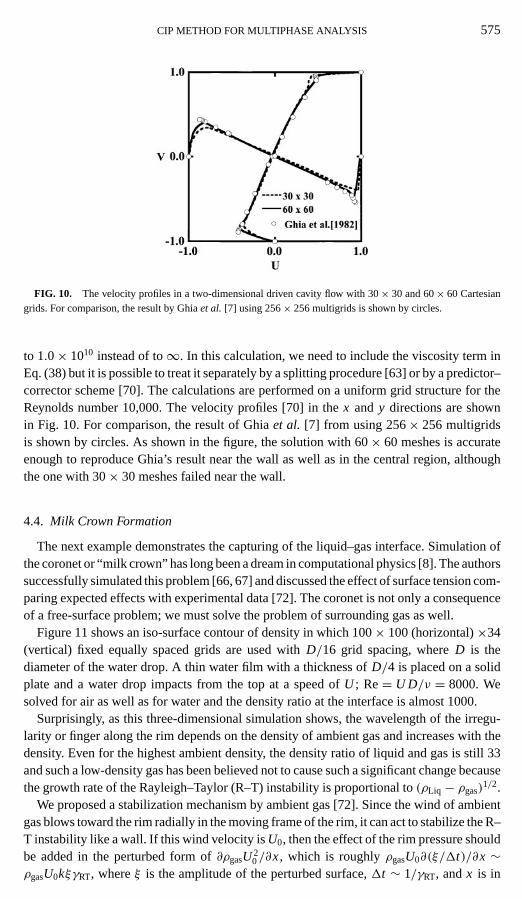
FIG. 10. The velocity profiles in a two-dimensional driven cavity flow with 30× 30 and 60× 60 Cartesiangrids. For comparison, the result by Ghiaet al. [7] using 256× 256 multigrids is shown by circles.
to 1.0× 10¹⁰ instead of to∞. In this calculation, we need to include the viscosity term inEq. (38) but it is possible to treat it separately by a splitting procedure [63] or by a predictor–corrector scheme [70]. The calculations are performed on a uniform grid structure for theReynolds number 10,000. The velocity profiles [70] in thex and y directions are shownin Fig. 10. For comparison, the result of Ghiaet al. [7] from using 256× 256 multigridsis shown by circles. As shown in the figure, the solution with 60× 60 meshes is accurateenough to reproduce Ghia’s result near the wall as well as in the central region, althoughthe one with 30× 30 meshes failed near the wall.
4.4. Milk Crown Formation
The next example demonstrates the capturing of the liquid–gas interface. Simulation ofthe coronet or “milk crown” has long been a dream in computational physics [8]. The authorssuccessfully simulated this problem [66, 67] and discussed the effect of surface tension com-paring expected effects with experimental data [72]. The coronet is not only a consequenceof a free-surface problem; we must solve the problem of surrounding gas as well.
Figure 11 shows an iso-surface contour of density in which 100× 100 (horizontal)×34(vertical) fixed equally spaced grids are used withD/16 grid spacing, whereD is thediameter of the water drop. A thin water film with a thickness ofD/4 is placed on a solidplate and a water drop impacts from the top at a speed ofU ; Re= U D/ν = 8000. Wesolved for air as well as for water and the density ratio at the interface is almost 1000.
Surprisingly, as this three-dimensional simulation shows, the wavelength of the irregu-larity or finger along the rim depends on the density of ambient gas and increases with thedensity. Even for the highest ambient density, the density ratio of liquid and gas is still 33and such a low-density gas has been believed not to cause such a significant change becausethe growth rate of the Rayleigh–Taylor (R–T) instability is proportional to(ρLiq − ρgas)
1/2.We proposed a stabilization mechanism by ambient gas [72]. Since the wind of ambient
gas blows toward the rim radially in the moving frame of the rim, it can act to stabilize the R–T instability like a wall. If this wind velocity isU0, then the effect of the rim pressure shouldbe added in the perturbed form of∂ρgasU2
0/∂x, which is roughlyρgasU0∂(ξ/1t)/∂x ∼ρgasU0kξγRT, whereξ is the amplitude of the perturbed surface,1t ∼ 1/γRT, andx is in
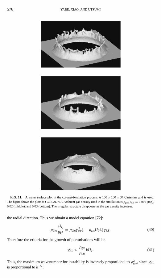
576 YABE, XIAO, AND UTSUMI
FIG. 11. A water surface plot in the coronet-formation process. A 100× 100× 34 Cartesian grid is used.The figure shows the plots att = 8.2D/U . Ambient gas density used in the simulation isρgas/ρLiq = 0.002 (top),0.02 (middle), and 0.03 (bottom). The irregular structure disappears as the gas density increases.
the radial direction. Thus we obtain a model equation [72]:
ρLiq∂2ξ
∂t2= ρLiqγ
2RTξ − ρgasU0kξγRT. (40)
Therefore the criteria for the growth of perturbations will be
γRT >ρgas
ρLiqkU0. (41)
Thus, the maximum wavenumber for instability is inversely proportional toρ2gas, sinceγRT
is proportional tok1/2.
CIP METHOD FOR MULTIPHASE ANALYSIS 577
In the simulation, we have included kinematic viscosity for water and air asU D/ν =8400 and 560, respectively. Since the viscosity effect appears in a form of kinematic viscosityin the R–T instability, the effect of the ambient density does not explicitly appear in theresult. The effect of surface tension has also been discussed in Ref. [72] and has beencompared to experimental results.
Since the wavelength of the fingers along the rim strongly depends on the density ofambient gas, the finger formation observed here is not an artifact of finite grid size, althoughit might have provided seeds of the instability. As is clear from this example, simulations canprovide important information about coronet-formation physics by modeling situations thatwould be hard to create experimentally. The phenomena observed here also give valuableinformation about GDI (gasoline direct injection) engines, in which the impact of splashingfuel on the combustion chamber is the key issue for efficient combustion [47] becauseof increasing surface area. Since ambient pressure in the chamber should be high, thegeneration of droplets might be greatly reduced as indicated here.
4.5. Laser-Induced Evaporation
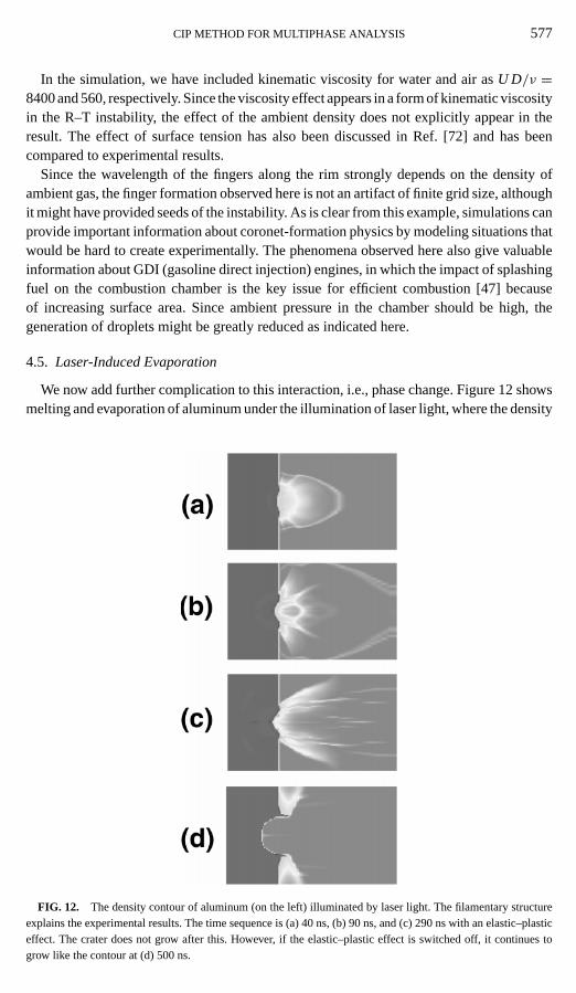
We now add further complication to this interaction, i.e., phase change. Figure 12 showsmelting and evaporation of aluminum under the illumination of laser light, where the density
FIG. 12. The density contour of aluminum (on the left) illuminated by laser light. The filamentary structureexplains the experimental results. The time sequence is (a) 40 ns, (b) 90 ns, and (c) 290 ns with an elastic–plasticeffect. The crater does not grow after this. However, if the elastic–plastic effect is switched off, it continues togrow like the contour at (d) 500 ns.

578 YABE, XIAO, AND UTSUMI
changes from 2.7 to 10−4 g/cm3. Aluminum solid is initially treated as an elastic material,whose treatment is given in Section 5, and then as a liquid and vapor during phase transition.This change is simple as realized by the equation of state shown in Fig. 9. This exampleshows that the code has a strong ability to describe a sharp interface and is robust enoughto treat both compressible and incompressible fluid simultaneously. In this calculation, weused two-dimensional cylindrical coordinates and a grid of 90 (axial)× 45 (radial). Laserlight is normally incident and is simply treated as a straight line depositing its energy at thesolid–gas interface with an absorption rate of 30%.
The experiment was performed at the Institute of Laser Engineering, Osaka University[68]. A YAG laser of 650 mJ and an 8-ns pulse width are used to illuminate an aluminum-slab target. Final crater depth and shape agree well with the simulation. It is interestingto note that the crater is not formed during the laser pulse but develops gradually over atime scale of several hundred nanoseconds well after the laser pulse has ended, as shownin Fig. 12. The very high temperature plasma of more than a few tens of electronvolts areproduced by the 8-ns laser pulse, and most of them expand from the target. However, somestay near the target for a long time after the laser pulse because of the recoil force fromexpanded plasmas and act as a heat source to melt the aluminum over a time scale of severalhundred nanoseconds.
When the plasma temperature becomes less than the melting temperature—around 290 ns(the time is measured from the laser peak)—aluminum with a strength of 0.248 Mbar and ayield strength of 2.2976 kbar starts being affected from the stress and no distortion occursafter that time. This yield stress plays an important role in determining the final crater size.Without yield strength, the crater develops further even after 490 ns and becomes severaltimes larger, as shown in Fig. 12d, although less difference is seen at the beginning around90 ns.
The plasma-heated crater formation leads to other interesting phenomena. Since theplasma acts not only as a heat source but also as a pressure source, the dynamic expansionof evaporated material at a later time is strongly modified. Since a high-pressure region isjust in front of the evaporation surface, the vapor is forced to bypass this region, flowingthrough a narrow channel between the metal surface and this pressure source. Therefore, thevapor preferentially flows toward a circumference with a large angle to the target normal.This effect is the exactly the same as that obtained in the experiment [68].
The simulation predicts additional interesting behavior. The expansion att < 40 ns isuniform because its temperature is high—a few tens of electronvolts. The experiment sup-ports this result and the debris around 0 degrees is very fine and indistinguishable withan optical microscope. On the other hand, the simulation result att = 290 ns shows somefilamentary streams flowing from the surface. The experiment also supports this result andthe debris at 75 degrees consists of particles of 1 to 20µm.
5. TREATMENT OF EMBEDDED BOUNDARIES IN CARTESIAN GRIDS
5.1. Fluid–Structure Interaction
Directly computing the interactions between solid bodies and suspended fluid is necessaryfor suspension flows in which the suspended bodies interact with the surrounding fluidand substantially influence the flow motion. An efficient computational model for flowscontaining distortionless rigid bodies can be constructed by using the numerical proceduresintroduced in Section 2.5.

CIP METHOD FOR MULTIPHASE ANALYSIS 579
Using color functions, we can easily treat solid bodies or objects that have any complexshape or heterogeneous density distributions.
The advection equation for the color functionφl ,
∂φl
∂t+ ub(l ) · ∇φl = 0, l = 1, 2, . . . , L , (42)
is solved by the method in Section 2.5 to recognize all the solid bodies, whereub(l ) is thevelocity field for objectl . The motion of the objectl is determined by
ub(l ) = ul + r × Ωl , (43)
whereul is the translational speed of the mass center of objectl , Ωl is the angular speed, andr is the distance to the mass center.r = x− X,X = ∫ xρφl dV/M , andM = ∫ ρφl dV.These quantities are predicted by Newton’s laws of motion
dul
dt= 1
M
∫dudtρφl dV, (44)
and
d
dt(Π(l )Ωl ) = Γl ≡
∫r × du
dtρφl dV, (45)
whereΓl is the torque for objectl . Π(l ) is the tensor of inertia moment≡ ∫ rr ρφl dV.All the forces (represented byρ du/dt, including both the body force and the fluid stress)
are calculated at all grids in a volume force form. It is convenient to compute the net forceon the mass center of objectl by summing up all the forces over the entire domain, butonly the region recognized byφl = 1 contributes to the integration in Eqs. (44) and (45).Different from the so-called “surface force” formulation, the volume force–based schemes,as we used here, do not need information about the body surface, such as orientations andsurface areas, which appears in other difficult problems in computation.
A non-slip condition is used to impose solid motion onto the velocity field of the fluid,which in turn is driven through the velocity coupling as
dudt= −ν
∑l
φl (u− ub(l )). (46)
Ths slip boundary condition can be treated similarly but is slightly more complicated [69].We computed a solid object undergoing steady translation at a low speedvs in Stokes
flows. Some similar examples can also be found in the works of Pan and Banerjee [25,26]. The Reynolds number Re= 2avs/ν is 0.006, wherea is the radius being described bytwo grids in Cartesian coordinates. Figure 13 shows the velocity component perpendicularto the velocity of the particle and the analytical results at different levels apart from theparticle, and here we find agreement between the numerical results and the analyticalsolutions.
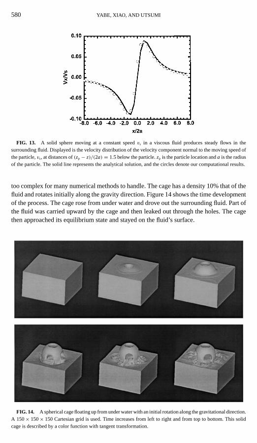
As an example of treating complex geometry, we simulated a rotating spherical cagerising from fluid under the force of floating. The cage is a hollow sphere with six holes onthe surface, and the thickness of the cage is described by seven grid sizes. This geometry is
580 YABE, XIAO, AND UTSUMI
FIG. 13. A solid sphere moving at a constant speedvs in a viscous fluid produces steady flows in thesurrounding fluid. Displayed is the velocity distribution of the velocity component normal to the moving speed ofthe particle,vs, at distances of(zp − z)/(2a) = 1.5 below the particle.zp is the particle location anda is the radiusof the particle. The solid line represents the analytical solution, and the circles denote our computational results.
too complex for many numerical methods to handle. The cage has a density 10% that of thefluid and rotates initially along the gravity direction. Figure 14 shows the time developmentof the process. The cage rose from under water and drove out the surrounding fluid. Part ofthe fluid was carried upward by the cage and then leaked out through the holes. The cagethen approached its equilibrium state and stayed on the fluid’s surface.
FIG. 14. A spherical cage floating up from under water with an initial rotation along the gravitational direction.A 150× 150× 150 Cartesian grid is used. Time increases from left to right and from top to bottom. This solidcage is described by a color function with tangent transformation.
CIP METHOD FOR MULTIPHASE ANALYSIS 581
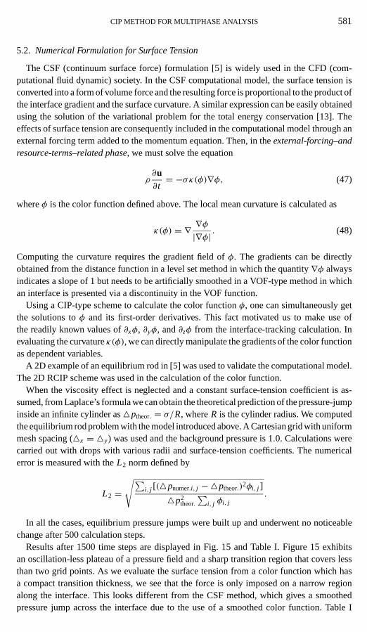
5.2. Numerical Formulation for Surface Tension
The CSF (continuum surface force) formulation [5] is widely used in the CFD (com-putational fluid dynamic) society. In the CSF computational model, the surface tension isconverted into a form of volume force and the resulting force is proportional to the product ofthe interface gradient and the surface curvature. A similar expression can be easily obtainedusing the solution of the variational problem for the total energy conservation [13]. Theeffects of surface tension are consequently included in the computational model through anexternal forcing term added to the momentum equation. Then, in theexternal-forcing–andresource-terms–related phase, we must solve the equation
ρ∂u∂t= −σκ(φ)∇φ, (47)
whereφ is the color function defined above. The local mean curvature is calculated as
κ(φ) = ∇ ∇φ|∇φ| . (48)
Computing the curvature requires the gradient field ofφ. The gradients can be directlyobtained from the distance function in a level set method in which the quantity∇φ alwaysindicates a slope of 1 but needs to be artificially smoothed in a VOF-type method in whichan interface is presented via a discontinuity in the VOF function.
Using a CIP-type scheme to calculate the color functionφ, one can simultaneously getthe solutions toφ and its first-order derivatives. This fact motivated us to make use ofthe readily known values of∂xφ, ∂yφ, and∂zφ from the interface-tracking calculation. Inevaluating the curvatureκ(φ), we can directly manipulate the gradients of the color functionas dependent variables.
A 2D example of an equilibrium rod in [5] was used to validate the computational model.The 2D RCIP scheme was used in the calculation of the color function.
When the viscosity effect is neglected and a constant surface-tension coefficient is as-sumed, from Laplace’s formula we can obtain the theoretical prediction of the pressure-jumpinside an infinite cylinder as4ptheor. = σ/R, whereR is the cylinder radius. We computedthe equilibrium rod problem with the model introduced above. A Cartesian grid with uniformmesh spacing (4x = 4y) was used and the background pressure is 1.0. Calculations werecarried out with drops with various radii and surface-tension coefficients. The numericalerror is measured with theL2 norm defined by
L2 =√∑
i, j [(4pnumer.i, j −4ptheor.)2φi, j ]
4p2theor.
∑i, j φi, j
.
In all the cases, equilibrium pressure jumps were built up and underwent no noticeablechange after 500 calculation steps.
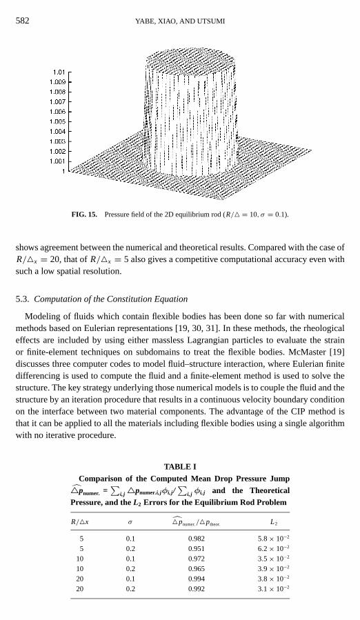
Results after 1500 time steps are displayed in Fig. 15 and Table I. Figure 15 exhibitsan oscillation-less plateau of a pressure field and a sharp transition region that covers lessthan two grid points. As we evaluate the surface tension from a color function which hasa compact transition thickness, we see that the force is only imposed on a narrow regionalong the interface. This looks different from the CSF method, which gives a smoothedpressure jump across the interface due to the use of a smoothed color function. Table I
582 YABE, XIAO, AND UTSUMI
FIG. 15. Pressure field of the 2D equilibrium rod (R/4 = 10, σ = 0.1).
shows agreement between the numerical and theoretical results. Compared with the case ofR/4x = 20, that ofR/4x = 5 also gives a competitive computational accuracy even withsuch a low spatial resolution.
5.3. Computation of the Constitution Equation
Modeling of fluids which contain flexible bodies has been done so far with numericalmethods based on Eulerian representations [19, 30, 31]. In these methods, the rheologicaleffects are included by using either massless Lagrangian particles to evaluate the strainor finite-element techniques on subdomains to treat the flexible bodies. McMaster [19]discusses three computer codes to model fluid–structure interaction, where Eulerian finitedifferencing is used to compute the fluid and a finite-element method is used to solve thestructure. The key strategy underlying those numerical models is to couple the fluid and thestructure by an iteration procedure that results in a continuous velocity boundary conditionon the interface between two material components. The advantage of the CIP method isthat it can be applied to all the materials including flexible bodies using a single algorithmwith no iterative procedure.
TABLE I
Comparison of the Computed Mean Drop Pressure Jump
4pnumer. =∑
i, j4pnumer.i, jφi, j /∑
i, j φi, j and the Theoretical
Pressure, and theL2 Errors for the Equilibrium Rod Problem
R/4x σ 4pnumer./4ptheor. L2
5 0.1 0.982 5.8× 10⁻²
5 0.2 0.951 6.2× 10⁻²
10 0.1 0.972 3.5× 10⁻²
10 0.2 0.965 3.9× 10⁻²
20 0.1 0.994 3.8× 10⁻²
20 0.2 0.992 3.1× 10⁻²

CIP METHOD FOR MULTIPHASE ANALYSIS 583
Based on the fractional-step solution procedure mentioned in the previous sections, we canconstruct a numerical treatment for the constitutive equation–related phase [58] separatelyfrom other processes. The constitutive relation, which has a differential form and relates thevelocity to the stress or stress rate, is solved by the finite-difference method. The resultingvelocity is then used as a provisional value in the remaining computations.
Constitutive equations, which give prescribed relations between stress and strain, areusually expressed in terms of stress or stress rate and strain or strain rate. Since velocity isone of the dependent variables in the present computational model, a constitutive equationin terms of strain rate is more convenient to formulate. Thus an equation such as
dsi j
dt= 2G
(1
2
dεi j
dt− 1
3
dεkk
dtδi j
)dεi j
dt≡ ∂ui
∂xj+ ∂u j
∂xi
is used to obtain a stress tensorsi j from velocity fields with Young modulusG. By usinga staggered grid, the conventional central differencing results in a compact computationalformulation. The time integration of the “velocity–stress” relations can be computed by amultistep explicit scheme based on the Taylor expansion [58] or by a semi-implicit schemeusing the ADI (alternative directional implicit) technique [53].
Figure 16 shows the sequence of two kinds of viscoelastic bodies sedimenting in fluidunder the force of gravity. The object is initially put in a direction oblique to gravity whichpoints downward. Once released, the object moves down and is imposed on by forces fromthe surrounding fluid. As expected from the theoretical analysis [59], the net external forcealong the body will bend the long axis into a curve. The bent object will then produce atorque that tends to push it toward a horizontal position. Thus, the object vacillates while itis sedimenting in the fluid. A constitutive equation for a Hook elastic solid is used for thepure elastic body. As can be seen from Fig. 16 (top), the elastic force resists the forcing fromthe fluid and prevents further deformation of the body. For the Maxwell body, a constitutiveequation for a Maxwell solid body is used, which includes both elastic and viscous effects,and a relaxation on elastic stresses takes place. In the present calculation (Fig. 16, bottom),the Deborah number (ND = τ/te with te being the total integration time) is about 2/3. Thestress is released significantly during the computation. The body is bent to a larger extentand behaves more like fluid.
Figure 17 shows another example. An elastic ball collides with a plate which is fixed onboth sides. Both ball and plate move through a 100× 100 fixed Cartesian grid. Here only10 grids are used to describe the thickness of the plate at its initial location. The black partin the figure is filled with air and is also taken into account in the calculations. After thecollision, the ball again detached from the plate. Such behavior is difficult to simulate withadapted grid methods.
6. CONSERVATIVE SEMI-LAGRANGIAN SCHEMES
It is useful to look for conservative semi-Lagrangian schemes because the semi-Lagrangian method can be effective on parallel computers, is suitable for multiphase flow,and enables the advection calculation to be made with a large time step free from the CFLcondition. Although the semi-Lagrangian scheme has been successfully used in short-termatmospheric problems, the loss of exact conservation makes the scheme inappropriate forlong-term problems and oceanic problems.

584 YABE, XIAO, AND UTSUMI
FIG. 16. Sedimentation of a pure elastic body (top) and a Maxwell body (bottom) in fluid. Time increasesfrom left to right and from top to bottom. The vorticity of the environmental flow is also plotted.
Furthermore, some subjects require exact conservation of mass. A typical example isblack-hole formation and emission of gravity waves [36]. In this case, a small fraction ofmass is converted into gravity waves and strict mass conservation is essential. Anotherexample is plasma simulation in which a Vlasov equation in six-dimensional phase space

CIP METHOD FOR MULTIPHASE ANALYSIS 585
FIG. 17. Example of elastic–plastic flow. The system is described by a 100× 100 Cartesian fixed grid, andonly 10 grids are used for the width of the plate. The plate and ball are moving through a fixed-grid system. Theblack part is filled with air and is also taken into account in the calculations.
must be solved and total particle density must be conserved or else a large electric fieldappears. The CIP method can be constructed to exactly conserve the total mass in a Vlasovsystem of equally spaced grids in phase space [21]. However, the use of non-equally spacedgrids or other general grids can save on computational cost and is worthy of investigation.
In this sense, establishing exact conservation in a semi-Lagrangian form would be a chal-lenging task. In shall section, we propose a non-conservative or semi-Lagrangian schemethat guarantees exact mass conservation.
6.1. CIP–CSL4 [43]
We first discuss the conservation law, which is computed as
∂ f
∂t+ ∂(u f )
∂x= 0. (49)
As already seen, the CIP adopts an additional constraint, i.e., the spatial gradient, to representthe profile inside the grid cell. In order to ensure the conservative property, we here addanother constraint,
ρni+1/2 =
∫ xi+1
xi
f n dx. (50)
586 YABE, XIAO, AND UTSUMI
Therefore the spatial profile must be constructed to satisfy this additional constraint as well.If this is possible,f is advanced in the non-conservative form, but conservation is realizedby ρ which is advanced by remapping of the Lagrangian volume, as described below.
The i th function pieceFi (x) is determined so as to satisfy the continuity conditionFi (xi−1) = f (xi−1), Fi (xi ) = f (xi )
∂Fi (xi−1)/∂x = g(xi−1), ∂Fi (xi )/∂x = g(xi )∫ xi
xi−1Fi (x) dx = ρi−1/2.
(51)
In order to meet the above condition, a fourth-order polynomial can be chosen as an inter-polation functionFi (x); the time development off andg is calculated simply by shiftingthe interpolation functionFi (x) by u1t in the same way as Eq. (4) of the CIP method as
f ∗i = Fi(xi − un
i 1t) = an
i ξ4i + bn
i ξ3i + cn
i ξ2i + gn
i ξi + f ni , (52)
g∗i = ∂Fi(xi − un
i 1t)/∂x = 4an
i ξ3i + 3bn
i ξ2i + 2cn
i ξi + gni , (53)
whereξi = −uni 1t and
ani =−5(6( fiup+ fi )1xi − (giup− gi )1x2
i + 12sgn(un
i
)ρi−sgn(un
i )/2)
21x5i
,
bni =
4(7( fiup+ 8 fi )1xi − (giup− (3/2)gi )1x2
i + 15sgn(un
i
)ρi−sgn(un
i )/2)
1x4i
, (54)
cni =−3(4(2 fiup+ 3 fi )1xi − (giup− 3gi )1x2
i + 20sgn(uni )ρi−sgn(un
i )/2)
21x3i
,
1xi = xiup− xi ,
iup =
i − 1 if uni ≥ 0,
i + 1 if uni < 0,
sgn(un
i
) = +1 if uni ≥ 0,
−1 if uni < 0.
The problem left for us is to calculate the time development ofρ. If we define the upstreamdeparture point ofxi as
xpi = xi −
∫ t+1t
tui dt, (55)
the density contained between [xpi−1, xp
i ] is simply remapped into [xi−1, xi ] at t +1t .Therefore in the simplest case ofu1t/1x < 1, the time development ofρ is calculated bythe following equation.
ρn+1i−1/2 = ρn
i−1/2+1ρni−1−1ρn
i . (56)
With the aid of Fig. 18, it is clear that1ρni is defined by the equation
1ρni =
∫ xi
xi−uni 1t
Fni (x) dx = −
(an
i
5ξ4
i +bn
i
4ξ3
i +cn
i
3ξ2
i +gn
i
2ξi + f n
i
)ξi , (57)
whereξi = −uni 1t, and each coefficient is equivalent to Eq. (54) at time stepn.

CIP METHOD FOR MULTIPHASE ANALYSIS 587
FIG. 18. The inflow and outflow of flux during1t .
Therefore, the solution of Eq. (49) is given by Eqs. (52)–(57). Extension to more generalequations is similar to the CIP method.
6.2. Numerical Tests
We present some sample calculations to test the procedure given in the previous section.The first example is an advection with variable velocity and Eq. (49) is solved under a givenvelocity field,
u = 1+ 0.5 sin(2πx/100),
with the initial condition
f (0, x) =
1 if 40≤ x ≤ 60
0 otherwise,
where equally spaced grid points of1x = 100/(N − 1) and a time-step size of1t =10/(N − 1) are used,N being the number of grid points.
We repeated the calculation by changing the total number of grid points to 101, 301, and1001 to test grid dependence of the present scheme, the CIP scheme, the upwind scheme, andTVD with a superbee limiter [39], as shown in Fig. 19. The result of the first-order upwindscheme withN = 10,001 is also shown in Fig. 19. All profiles shown are after 10(N − 1)time steps, which corresponds tot = 100. Since no analytical solution is available, theresult of the present scheme withN = 1001 is shown by the solid line in the figure.
We confirm that the accuracy has been improved at the discontinuity by the presentscheme. Note that the first-order upwind scheme needs 10,001 grid points to obtain thesame result as the present scheme or the CIP method using 101 grid points, which convergesto one solution regardless of grid size. Furthermore, it has already been shown that mostof the modern schemes such as TVD and ENO fail to reproduce the result with 101 gridpoints [42], as shown in Fig. 19.
The following one-dimensional Burger’s equation is an interesting example of applicationto a non-linear equation.
∂u
∂t+ u
∂u
∂x= λ∂
2u
∂x2≡ S. (58)
The viscosity term is calculated with a finite-difference approach.

588 YABE, XIAO, AND UTSUMI
FIG. 19. Propagation of a square wave with a given velocity field by the present scheme, the CIP method,the upwind scheme, and the TVD scheme with a superbee limiter (SPB) at t= 100. The number of grids is 101(circles), 301 (triangles), 1,001 (squares), and 10,001 (diamonds). For comparison, the result of the present schemewith 1,001 grids is shown by the solid line.
In order to calculate the spatial derivative ofu, we differentiate Eq. (58); then
∂u′
∂t+ u
∂u′
∂x= −u′2+ S′. (59)
This equation is split into two phases:∂u′/∂t + u∂u′/∂x = 0 (advection) and∂u′/∂t =−u′2+ S′ (non-advection). We calculate the advection phase with Eq. (4), and the non-advection phase with the following equation, applying a finite-difference method.
u′n+1i = u′∗i − (u′∗i )21t.
The SandS′ terms are treated by the method given in Section 3.2. In fact, first-order timeintegration is not necessarily used here. A higher order integration along the trajectory canbe easily implemented.
For the calculation ofρ(≡∫ u dx), we transform Eq. (58) into the conservation form asfollows.
∂u
∂t+ ∂(u
2/2)
∂x= S. (60)

CIP METHOD FOR MULTIPHASE ANALYSIS 589
FIG. 20. The result of Burger’s equation without viscosity with the present scheme with 101 grid points att = 100. For comparison, the result of the first-order upwind scheme with 1001 grid points att = 100 is shownby the solid line.
Figure 20 shows the calculation result att = 100 withλ = 0 and the initial condition
u(0, x) = 0.5+ 0.4 cos(2πx/100), (61)
and equally spaced grid points of1x = 1.0, a time-step size of1t = 0.1, and mesh numberN = 101 are used.
In order to check the exact speed of a shock wave, we show the result of the calculationwith the conservative form of Burger’s equation using the first-order upwind scheme withN = 1001.
FIG. 21. The result of Burger’s equation with viscosity with the present scheme att = 100. The exact solutionis shown by the solid line.

590 YABE, XIAO, AND UTSUMI
FIG. 22. Bird’s-eye view of a gas–liquid turbulence mixing layer.
In this calculation, although the viscosity term is not considered, the speed of a shockwave can be exactly reproduced by the present scheme.
Next we solve Eq. (58) with a viscosity term and condition as
u(0, x) =
0.9 if x ≤ 10
−0.1 if x > 10,
where equally spaced grid points of1x = 1, and a time-step size of1t = 0.1 are used.The coefficient of the viscosity term is set toλ = 0.15.
Figure 21 shows the profile after 1000 time steps that corresponds tot = 10, and thepropagation speed agrees well with the exact solution.
7. SUMMARY
We have reviewed various families of the CIP method to address the problem of multi-phase flow. Significant improvements are still being made but we cannot discuss all of thoseefforts, such as, application to the finite-element method, extension to higher order polyno-mials, application to other equations such as diffusion or the Poisson equation. Applicationof the CIP method to various fields such as volcanic eruption, astrophysical jets [17], theGDI engine, and combustion is also expanding. Some of these fields are discussed in thespecial issue of the CFD Journal on the CIP method (vol. 8, No. 1, 1999). Before closing,we introduce an interesting application done by Mutsuda and Yasuda [20]. Figure 22 showsa bird’s-eye view of a gas–liquid turbulence mixing layer driven by jet ejection, in whicha three-dimensional domain of a solitary wave leads to very forceful wave-breaking on adouble reef with two steps, and the surface profiles and entrained air bubble motions developquickly into the turbulent mixing layer with strong three-dimensionality. This simulationhas been done with one CPU on an Intel-based personal computer (with a 300-MHz PentiumII processor).
REFERENCES
1. A. A. Amsden and F. H. Harlow, A simplified MAC technique for incompressible fluid flow calculations,J. Comput. Phys.6, 322 (1970).
2. T. Aoki, Multi-dimensional advection of CIP (cubic-interpolated propagation) scheme,CFD J.4, 279 (1995).
3. J. B. Bell and D. L. Marcus, A second-order projection method for variable-density flows,J. Comput. Phys.101, 334 (1992).

CIP METHOD FOR MULTIPHASE ANALYSIS 591
4. R. Bermejo and A. Staniforth, The conversion of semi-Lagrangian advection schemes to quasi-monotoneschemes,Mon. Weather Rev.120, 2622 (1992).
5. J. U. Brackbill, D. B. Kothe, and C. Zemach, A continuum method for modeling surface tension,J. Comput.Phys.100, 335 (1992).
6. P. Colella and P. R. Woodward, The piecewise parabolic method (PPM) for gas-dynamical simulations,J. Comput. Phys.54, 174 (1984).
7. U. Ghia, K. N. Ghia, and C. T. Shin, High-resolution for incompressible flow using the Navier-Stokes equationsand a multi-grid method,J. Comput. Phys.48, 387 (1982).
8. F. H. Harlow and J. P. Shannon, The splash of a liquid drop,J. Appl. Phys.38, 3855 (1967).
9. F. H. Harlow and A. A. Amsden, Numerical simulation of almost incompressible flow,J. Comput. Phys.3,80 (1968).
10. F. H. Harlow and J. E. Welch, Numerical calculation of time-dependent viscous incompressible flow with freesurface,Phys. Fluids8, 2182 (1965).
11. C. W. Hirt and B. D. Nichols, Volume of fluid (VOF) method for the dynamics of free boundaries,J. Comput.Phys.39, 201 (1981).
12. R. I. Issa, Solution of the implicitly discretised fluid flow equations by operator-splitting,J. Comput. Phys.62, 40 (1985).
13. D. Jacqmin, A variational approach to deriving smeared interface surface tension models, inBarriers andChallenges in CFD, edited by V. Venkatakrishnanet al.(Kluwer Academic, Dordrecht/Norwell, MA, 1998),p. 231.
14. K. C. Karki and S. V. Patankar, Pressure-based calculation procedure for viscous flows at all speeds in arbitraryconfigurations,AIAA J.27, 1167 (1989).
15. S. Karni, Multicomponent flow calculations by a consistent primitive algorithm,J. Comput. Phys.112, 31(1994).
16. D. B. Kothe, W. J. Rider, S. J. Mosso, and J. S. Brock,Volume tracking of interfaces having surface tensionin two and three dimensions, AIAA Paper 96-0859, 1996.
17. T. Kudoh, R.Matsumoto, and K.Shibata, Magnetically driven jets from accretion disks. III. 2.5-dimensionalnonsteady simulations for thick disk case,Astrophys. J.508, 186 (1998).
18. C. E. Leith, Numerical simulation of the earth’s atmosphere, inMethods in Computational Physics, Vol. 4,edited by B. Alderet al. (Academic Press, New York, 1965), p. 1.
19. W. H. McMaster,1984 Computer codes for fluid-structure interactions, Lawrence Livermore LaboratoryReport UCRL-89724, 1984.
20. H. Mutsuda and T. Yasuda, Physical mechanism based on numerical simulations of strongly turbulent air-watermixing layer within surf-zone,Proceedings 27th Int. Conf. on Coastal Eng., Sydney, 1999.
21. T. Nakamura and T. Yabe, Cubic interpolated propagation scheme for solving the hyper-dimensional Vlasov-Poisson equation in phase space,Comput. Phys. Commun.120, 122 (1999).
22. J. Von Neumann and R. D. Richtmyer, A method for the numerical calculation of the hydrodynamic shocks,J. Appl. Phys.21, 232 (1950).
23. Y. Ogata and T. Yabe, Shock capturing with improved numerical viscosity in primitive Euler representation,Comput. Phys. Commun.119, 179 (1999).
24. S. Osher and J. A. Sethian, Front propagating with curvature-dependent speed: Algorithms based on Hamilton-Jacobi formulations,J. Comput. Phys.79, 12 (1988).
25. Y. Pan and S. Banerjee, Numerical simulation of particle interactions with wall turbulence,Phys. Fluids8,2733 (1996).
26. Y. Pan and S. Banerjee, Numerical investigation of the effects of large particles on wall-turbulence,Phys.Fluids9, 3786 (1997).
27. S. V. Patanker,Numerical Heat Transfer and Fluid Flow(McGraw–Hill, New York, 1980).
28. S. V. Patanker and D. B. Spalding, A calculation procedure for heat, mass and momentum transfer in three-dimensional parabolic flows,Int. J. Heat Mass Transfer15, 1787 (1972).
29. D. Peng, B. Merriman, S. Osher, H. K. Zhao, and M. Kang, A PDE-based fast local level-set method,J. Comput.Phys.155, 410 (1999).
592 YABE, XIAO, AND UTSUMI
30. C. S. Peskin, Numerical analysis of blood flow in the heart,J. Comput. Phys.25, 220 (1977).
31. C. S. Peskin and D. M. McQueen, A three-dimensional computational model for blood flow in the heart. I.Immersed elastic fibers in viscous incompressible fluid,J. Comput. Phys.81, 372 (1989).
32. E. G. Puckett, A. S. Almgren, J. B. Bell, D. L. Marcus, and W. J. Rider, A high-order projection method fortracking fluid interfaces in variable density incompressible flows,J. Comput. Phys.130, 269 (1997).
33. E. G. Puckett and J. S. Saltzman, A 3D adaptive mesh refinement algorithm for multimaterial gas dynamics,Physica D60, 84 (1992).
34. D. K. Purnell, Solution of the advective equation by upstream interpolation with a cubic spline,Mon. WeatherRev.104, 42 (1975).
35. W. J. Rider and D. B. Kothe,Stretching and Tearing Interface Tracking Methods, AIAA-95-1717, 33rdAerospace Sciences Meeting and Exhibit, Reno, 1995.
36. S. L. Shapiro and S. A. Teukolsky,Black Holes, White Dwarfs, and Neutron Stars(Wiley, New York, 1983).
37. A. Staniforth and J. Cˆote, Semi-Lagrangian integration scheme for atmospheric model—A review,Mon.Weather Rev.119, 2206 (1991).
38. M. Sussman, P. Smereka, and S. Osher, A level set approach for computing solutions to incompressibletwo-phase flow,J. Comput. Phys.114, 146 (1994).
39. P. K. Sweby, High-resolution schemes using flux limiters for hyperbolic conservation laws,SIAM J. Numer.Anal.21, 995 (1984).
40. H. Takewaki, A. Nishiguchi, and T. Yabe, The cubic-interpolated pseudo-particle (CIP) method for solvinghyperbolic-type equations,J. Comput. Phys.61, 261 (1985).
41. H. Takewaki and T. Yabe, Cubic-interpolated pseudo particle (CIP) method—application to nonlinear ormulti-dimensional problems,J. Comput. Phys.70, 355 (1987).
42. R. Tanaka, T. Nakamura, T. Yabe, and H. Wu, A class of conservative formulation of the CIP method,CFDJ. 8, 1 (1999).
43. R. Tanaka, T. Nakamura, and T. Yabe, Constructing an exactly conservative scheme in a non-conservativeform, Comput. Phys. Commun.126, 232 (2000).
44. E. T. Toro, Riemann Solvers and Numerical Methods for Fluid Dynamics(Springer-Verlag, Berlin,1997).
45. S. O. Unverdi and G. A. Tryggvasson, A front-tracking method for viscous, incompressible, multi-fluid flows,J. Comput. Phys.100, 25 (1992).
46. T. Utsumi, T. Kunugi, and T. Aoki, Stability and accuracy of the cubic interpolated propagation scheme,Comput. Phys. Commun.101, 9 (1996).
47. T. Wakisaka, S. Takeuchi, and J. H. Chung, A numerical study on the mixture formation process in fuelinjection engines by means of the CIP method,CFD J.8, 82 (1999).
48. P. Y. Wang, T. Yabe, and T. Aoki, A general hyperbolic solver—the CIP method—applied to curvilinearcoordinates,J. Phys. Soc. Japan62, 1865 (1993).
49. M. L. Wilkins, Use of artificial viscosity in multidimensional fluid dynamic calculations,J. Comput. Phys.36, 281 (1980).
50. M. L. Wilkins,Computer Simulation of Dynamic Phenomena(Springer-Verlag, New York 1999).
51. D. L. Williamson and P. J. Rasch, Two-dimensional semi-Lagrangian transport with shape-preserving inter-polation,Mon. Weather Rev.117, 102 (1989).
52. P. R. Woodward and P. Colella, The numerical simulation of two-dimensional fluid flow with strong shocks,J. Comput. Phys.54, 115 (1984).
53. F. Xiao,Numerical Scheme for Advection Equation and Multi-Layered Fluid Dynamics, Ph.D thesis (TokyoInstitute of Technology, 1996).
54. F. Xiao, T. Yabe, and T. Ito, Constructing an oscillation-preventing scheme for the advection equation by arational function.Comput. Phys. Commun.93, 1 (1996).
55. F. Xiao, T. Yabe, G. Nizam, and T. Ito, Constructing a multi-dimensional oscillation-preventing scheme forthe advection equation by a rational function,Comput. Phys. Commun.94, 103 (1996).
56. F. Xiaoet al., An Efficient model for driven flow and application to a gas circuit breaker,Comput. Model.Sim. Eng.1, 235 (1996).
CIP METHOD FOR MULTIPHASE ANALYSIS 593
57. F. Xiao, T. Yabe, T. Ito, and M. Tajima, An algorithm for simulating solid objects suspended in stratified flow,Comput. Phys. Commun.102, 147 (1997).
58. F. Xiao and T. Yabe, Computation of complex flows containing rheological bodies,CFD J.8, 43 (1999).
59. X. Xu and A. Nadim, Deformation and orientation of an elastic slender body sedimenting in viscous liquid,Phys. Fluids6, 2889 (1994).
60. T. Yabe and E. Takei, A new higher-order Godunov method for general hyerbolic equations,J. Phys. Soc.Japan57, 2598 (1988).
61. T. Yabe and T. Aoki, A universal solver for hyperbolic-equations by cubic-polynomial interpolation. I. One-dimensional solver,Comput. Phys. Commun.66, 219 (1991).
62. T. Yabe, T. Ishikawa, P. Y. Wang, T. Aoki, Y. Kadota, and F. Ikeda, A universal solver for hyperbolic-equationsby cubic-polynomial interpolation. II. Two- and three-dimensional solvers,Comput. Phys. Commun.66, 233(1991).
63. T. Yabe and P. Y. Wang, Unified numerical procedure for compressible and incompressible fluid,J. Phys. Soc.Japan60, 2105 (1991).
64. T. Yabe and F. Xiao, Description of complex and sharp interface during shock wave interaction with liquiddrop,J. Phys. Soc. Japan62, 2537 (1993).
65. T. Yabe and F. Xiao, Description of complex and sharp interface with fixed grids in incompressible andcompressible fluid,Computer Math. Applic.29, 15 (1995).
66. T. Yabe, Interface capturing and universal solution of solid, liquid and gas by CIP method,Proceedings Conf.High-Performance Computing on Multi-phase Flow, Tokyo, 1997.
67. T. Yabe, Y. Zhang, and F. Xiao, A numerical procedure—CIP—to solve all phases of matter together,LectureNote in Physics, Sixteenth Int. Conf. on Numerical Methods in Fluid Dynamics, (Springer-Verlag, New York,1998), p. 439.
68. T. Yabe, Simulation of laser-induced melting and evaporation dynamics by the unified solver CIP for solid,liquid and gas, inMathematical Modeling of Weld Phenomena 4, edited by H. Cerjak (cambridge Univ. Press,Cambridge, U.K., 1998), p. 26.
69. T. Yabe, F. Xiao, and Y. Zhang,Strategy for unified solution of solid, liquid, gas and plasmas, AIAA PaperNo. 99-3509, 30th AIAA Fluid Dynamics Conference, Norfolk, 1999.
70. S. Y. Yoon and T. Yabe, The unified simulation for incompressible and compressible flow by the predictor–corrector scheme based on the CIP method,Comput. Phys. Commun.119, 149 (1999).
71. D. L. Youngs, Time-dependent multi-material flow with large fluid distortion, inNumerical Methods for FluidDynamics, edited by K. W. Morton and M. J. Baines (Academic Press, New York, 1982), p. 273.
72. Y. Zhang and T. Yabe, Effect of ambient gas on three-dimensional breakup in coronet formation,CFD J. 8,378 (1999).
73. O. C. Zienkiewicz and J. Wu, A general explicit or semi-explicit algorithm for compressible and incompressibeflows, Int. J. Num. Meth. Eng.35, 457 (1992).
74. S. T. Zalesak, Fully multidimensional flux-corrected transport algorithm for fluids,J. Comput. Phys.31, 335(1979).