the earth’s magnetic field - heim | skemman ·...

Physics DepartmentHáskóli Íslands

2012

Physics DepartmentHáskóli Íslands

2012

The Earth’s Magnetic Field

Edda Lína Gunnarsdóttir

THE EARTH’S MAGNETIC FIELD

Edda Lína Gunnarsdóttir

10 ECTS unit research project, part of aBaccalaureus Scientiarum degree in Physics

InstructorGunnlaugur Björnsson

Physics DepartmentSchool of Engineering and Natural Sciences

Univerity of IcelandReykjavik, June 2012

The Earth’s Magnetic Field10 ECTS unit research project, part of a B.Sc. degree in Physics

Copyright c© 2012 Edda Lína GunnarsdóttirAll rights reserved.

Physics DepartmentSchool of Engineering and Natural SciencesUniversity of IcelandHjarðarhagi 6101, ReykjavikIceland

Telephone: 525 4000

Registration information:Edda Lína Gunnarsdóttir, 2012, The Earth’s Magnetic Field, Research Project, PhysicsDepartment, University of Iceland.

ISBN XX

Printing: Háskólaprent, Fálkagata 2, 107 ReykjavíkReykjavik, Iceland, June 2012

Abstract

The Earth’s magnetic field is essential for life on Earth, as we know it, to exist. Itforms a magnetic shield around the planet, protecting it from high energy particlesand radiation from the Sun, which can cause damage to life, power systems, orbitingsatellites, astronauts and spacecrafts. This report contains a general overview of theEarth’s magnetic field. The different sources that contribute to the total magneticfield are presented and the diverse variations in the field are described. Finally, mea-surements of the Earth’s magnetic field are introduced and the applied instrumentsand procedures described, with an emphasis on Leirvogur magnetic observatory.

Contents

List of Figures ix

List of Tables 1

1 Introduction 3

2 Properties and Origin 52.1 Contributions to the Total Magnetic Field . . . . . . . . . . . . . . . 52.2 The Elements of the Earth’s Magnetic Field . . . . . . . . . . . . . . 62.3 The Geometry of the Earth’s Magnetic Field . . . . . . . . . . . . . . 7

2.3.1 Spherical Harmonic Description . . . . . . . . . . . . . . . . . 82.4 The Magnetosphere . . . . . . . . . . . . . . . . . . . . . . . . . . . . 13

3 Time Variations 173.1 Long Term Variations . . . . . . . . . . . . . . . . . . . . . . . . . . . 183.2 Short Term Variations . . . . . . . . . . . . . . . . . . . . . . . . . . 20

3.2.1 Irregular Variations . . . . . . . . . . . . . . . . . . . . . . . . 203.2.2 The Active Sun . . . . . . . . . . . . . . . . . . . . . . . . . . 233.2.3 Regular Variations . . . . . . . . . . . . . . . . . . . . . . . . 24

4 Measurements 274.1 Geomagnetic Observatories . . . . . . . . . . . . . . . . . . . . . . . . 294.2 Magnetometers . . . . . . . . . . . . . . . . . . . . . . . . . . . . . . 32

4.2.1 Fluxgate Magnetometers . . . . . . . . . . . . . . . . . . . . . 344.2.2 Proton Precession Magnetometer . . . . . . . . . . . . . . . . 374.2.3 Absolute Measurements . . . . . . . . . . . . . . . . . . . . . 37

5 Summary and Conclusions 41

Bibliography 43

vii

List of Figures

2.1 The elements of the Earth’s magnetic field. . . . . . . . . . . . . . . . 7

2.2 To a first approximation, the Earth’s magnetic field is like the fieldof a magnetic dipole. . . . . . . . . . . . . . . . . . . . . . . . . . . . 8

2.3 Spherical coordinate system with an origin at the Earth’s center, withrespect to a Cartesian coordinate system. . . . . . . . . . . . . . . . . 9

2.4 The total intensity, I, and the declination, D, of the main field in 2010. 12

2.5 The Earth’s magnetosphere and its characteristic regions. . . . . . . . 13

2.6 The solar wind blowing towards the Earth, shaping the magnetosphere. 14

2.7 Electric currents in the magnetosphere represented by red lines andthe blue lines represent magnetic fields. . . . . . . . . . . . . . . . . . 15

3.1 The drift of the north and south magnetic and geomagnetic poles. . . 19

3.2 Magnetogram from Leirvogur observatory showing a geomagnetic storm. 21

3.3 Coronal Mass Ejection (CME). Picture taken by the SOHO satellite. 24

3.4 The diurnal variation of the magnetic field components D, H and Zon solar quiet days (Sq variations), observed at different latitudes. . . 25

3.5 The total number of time intervals with K-index larger than or equalto 7. . . . . . . . . . . . . . . . . . . . . . . . . . . . . . . . . . . . . 26

4.1 The worldwide distribution of repeat stations since 1900. . . . . . . . 29

4.2 The layout of Leirvogur magnetic observatory. . . . . . . . . . . . . . 31

ix

LIST OF FIGURES

4.3 Photograph of Leirvogur magnetic observatory. . . . . . . . . . . . . . 31

4.4 Global distribution of geomagnetic observatories that particpated inINTERMAGNET as of January 2010 . . . . . . . . . . . . . . . . . . 32

4.5 The adopted baselines at Leirvogur magnetic observatory in 2010. . . 34

4.6 Fluxgate sensor. . . . . . . . . . . . . . . . . . . . . . . . . . . . . . . 35

4.7 Suspended triaxial fluxgate magnetometer. . . . . . . . . . . . . . . . 36

4.8 DI fluxgate theodolite and the scales of a theodolite. . . . . . . . . . 36

4.9 The scheme of an absolute measurement. . . . . . . . . . . . . . . . . 38

x

List of Tables

3.1 Standard scale for conversion between maximum intensity in the hor-izontal components, H and D, and the K-indices. . . . . . . . . . . . 18

1

1 Introduction

The Earth’s magnetic field has existed since the planet’s early days - long beforelife on Earth began. Without the magnetic field, life on Earth, as we know it, couldnot even exist. That is because the Earth’s magnetic field protects the near-Earthenvironment from dangerous radiation and high energy plasma from the Sun bypartially blocking it out. However, there is always some part of the plasma andradiation that is able to penetrate through the magnetic field barrier, and this oftenleads to magnetic disturbances around the Earth. Before humans started seekingout into space, with orbiting satellites and space voyages, and before electricitybecame a basic need of a daily life, the magnetic disturbances did not have a largeeffect on life on Earth. In modern times, the need to understand the behavior of theEarth’s magnetic field, its origin and variations, is becoming ever more important.With intense research, focused on both the surface of Earth, and the Sun-Earthenvironment, the goal is to be able to predict the behavior of the magnetic field,just as meteorologists predict the weather.

The intention of this report is to give a general overview of the Earth’s magnetic fieldby specifying its main properties, the characteristics of the magnetic field variationsand their causes. Included is also an introduction to the measurements of the Earth’smagnetic field, which are mainly carried out at magnetic observatories, and theinstruments used for measuring it. This report is hopefully suitable, not only, forsomeone stepping their first steps in the field of geomagnetism, but also for someoneworking within the field, wanting to refresh their memory on the basics.

To begin with, the geomagnetic field is introduced by describing the different sourcesof the observed magnetic field. One chapter is dedicated to variations in the magneticfield and their origins. From there, the emphasis moves to the subject of measuringthe magnetic field, describing the involved instruments and standard geomagneticobservatories, where the measurements are carried out.

3

2 Properties and Origin

The Earth has a magnetic field which is mainly produced within its interior andforms a protecting shield around the planet, called the magnetosphere. The mag-netosphere protects Earth’s inhabitants from the highly energetic and dangerousparticles from the sun and it prevents the Earth’s atmosphere from being blownaway by the solar wind.1 The geomagnetic field is thought to have existed muchfurther back in time than life on Earth. According to magnetized rocks as old as 4billion years, found in Greenland and Australia, the magnetic field already existedin the beginning of Earth’s history [8].

2.1 Contributions to the Total Magnetic Field

The observed magnetic field on Earth is called the geomagnetic field. It is a super-position of magnetic fields generated by different sources. The field generated by amagnetic dynamo in the Earth’s liquid core is called the main field and is by farthe most dominant one. The main field and the crustal field, which is generated bymagnetized rocks on the Earth’s crust, are categorized as the internal field and arerather stable in time compared to the external field. The external field is composedof the field produced by the electric currents in the ionosphere and magnetosphere.There is also a magnetic field produced by the induced currents in the crust, mantleand oceans which adds to the total geomagnetic field. To summarize, the geomag-netic field components which make up the total geomagnetic field are: The mainfield, the external field and the induced field.

A detailed global coverage of the magnetic field, for a long period of time, is neededfor it to be possible to separate and identify the different contributions of each partof the field to the total geomagnetic field. As mentioned above, the main field isproduced in the interior of the Earth by a self sustaining dynamo which is explainedby dynamo theory [8, 15]. Without going into details about the origin of the mainfield, the following basic description is made. The Earth’s core is believed to bemainly composed of iron (and to a smaller proportion, nickel) and consist of a solid

1It is thought that Mars had a denser atmosphere when it had a stronger magnetic field and thatit got blown away by the solar wind when the magnetic field became weak.

5


inner core and liquid outer core. The magnetic field is produced by circulatingelectric currents in the the highly conductive outer core. The complex motion of thecurrents (or the fluid conducting material), is driven by convection and the rotationof the Earth.2 The energy needed to sustain this dynamo is believed to be producedby solidification; when the heaviest elements in the fluid core freeze onto the solidcore and lighter elements are released, causing a convection [8].The non-homogeneityof the electric currents causes regional magnetic anomalies on the Earth’s surfaceand variations in the main field are connected to variations in the fluid velocity [8].Before the theory of a non-trivial dynamo in Earth’s interior, there were suggestionsthat the Earth’s magnetic field was produced by a strong permanent magnet locatedin its center. However, ferromagnetic material, like iron in the Earth’s core, cannotbe magnetized above their Curie temperature, the temperature at which a magnetlooses its magnetism. The temperature in the Earth’s core is much higher than theCurie temperature of iron. In fact, at the depth of a few tens of km3 the temperatureis higher than the Curie temperature of almost all known ferromagnetic materials[5]. According to this there must be electric currents in Earth’s interior producingthe field. At present time, the dynamo theory has come quite far. Computer modelsof the dynamo in the Earth’s core are being developed, and are able to simulatephenomena like the reversal of the poles, where north and south magnetic poles areinterchanged, and the slow changes in the main field.

2.2 The Elements of the Earth’s Magnetic Field

The geomagnetic field has a direction and magnitude at every point in space andthus is a vector field. Three parameters are needed to describe the magnetic fieldvector, F, at a point, P , on the Earth’s surface. The point, P , is assumed to besituated at the center of a Cartesian coordinate system with the x-axis directedtowards the geographic north, the y-axis directed to the east and the z-axis verticaland positive downwards into the Earth. The north, east and downward componentsof the field vector are denoted X, Y and Z. Figure 2.1 describes the geometry.A common way to describe the magnetic field is to specify the total intensity ofthe field F , the inclination, I, and the declination, D. The inclination is the anglefrom the horizontal plane to the vector and the declination is the angle from thex-axis to the component H, which is the horizontal component of F. Another wayof describing the magnetic field, is by specifying H, the vertical component Z, andthe declination, D. Figure 2.1 shows the orientation of each component and the

2The relatively fast rotation of the Earth is believed to play a key role in the Earth’s magnetic fieldand the dynamo in its core because the neighboring planet Venus has a similar core structurebut a slower rotation and thus doesn’t have a magnetic field [6].

3For comparison, the radius of Earth is approximately 6400 km.

6

2.3 The Geometry of the Earth’s Magnetic Field

following equations describe their internal relations:

F =√X2 + Y 2 + Z2, H =

√X2 + Y 2, I =arctanZ/H, D =arctanY/X.

The components in Cartesian coordinates are:

X =H cosD, Y =H sinD, Z =F sin I.

The geomagnetic field components X, Y, Z and H are given in nano teslas (nT)

Figure 2.1: The elements of the Earth’s magnetic field. F is the total intensityof the field, H is the horizontal component of F , D is the declination and I theinclination [8].

while the I and D are presented in degrees, arcmininutes and arcseconds which areall units of angular measurements, an arcminute being 1/60 of one degree and anarcsecond is 1/60 of one arcminute. A common way for magnetic observatories topresent their daily measurements is through a magnetogram. A magnetogram isa plot of the magnetic field versus time. Most often, three field components arespecified and the time interval used is 24 hours.


The absolute strength of the magnetic field on Earth’s surface varies from 23,000 nTto 62,000 nT [13].It is strongest around the poles and weakest around the equator butbetween the two, the variations in the strength is not linear. The field both varieswith space and time, and in this section the focus is on the spatial description andrepresentation of the Earth’s magnetic field. Short and long term time variations arediscussed in the next section. In the polar regions the magnetic field consists more

7


or less of a vertical component and at the equator the field lines lie in the horizontalplane. The location at which the field is purely vertical are called south and northmagnetic poles and they are not the same as the geographical poles marked by theEarth’s rotation axis.4 As implied, the Earth’s magnetic field is like the field of amagnetic dipole, but only to a first approximation.5 It is as if there were a giant

Figure 2.2: To a first approximation, the Earth’s magnetic field is like the field of amagnetic dipole [18].

bar magnet located at the center of the planet, tilted 11.5◦ degrees from the Earth’srotational axis. The hypothetical bar magnet should be oriented as shown in Figure2.2 since a compass points north and opposite poles attract. The locations wherethe magnetic poles would be if the Earth’s magnetic field was purely dipolar andproduced solely by a bar magnetic are called the geomagnetic poles. The location ofthe geomagnetic poles can be seen in figure 3.1. The simple and time independentbar magnet model does not take into account the many complex properties of themagnetic field, for instance magnetic anomalies, the field reversal, movement of thegeomagnetic poles and other variations in the field, which will be introduced later.An example of the deviations from a dipole field is the fact that the magnetic polesare not located exactly opposite each other.

2.3.1 Spherical Harmonic Description

An analytical expression of the global magnetic field is achieved by the use of spher-ical harmonics which come from the solution of Laplace’s equation. Therefore itis relevant to start by deriving Laplace’s equation. The two Maxwell’s equationsrelated to the magnet field are

∇ ·B = 0 , (2.1)

and∇×H = µ(J+

∂D

∂t) , (2.2)

4Another definition is the geomagnetic poles which are the locations where the magnetic poleswould be if the Earth’s magnetic field was purely dipolar and produced solely by a bar magnet.

5More than 90% of the observed field can be approximated by the simple dipole model [5].

8


where H is the magnetic field, B is the magnetic induction, J is the electric currentdensity and ∂D/∂t is the electric displacement current density. Given the approx-imation that there are no electric currents on the Earth’s surface,6 equation 2.2becomes ∇ × H = 0. As a consequence, the magnetic field, H, is a conservativevector field and can be connected to a magnetic scalar potential, V , by

H = −∇V. (2.3)

At the Earth’s surface the magnetic induction is B = µ0H, where µ0 is the perme-ability of free space. Now equation 2.3 and 2.1 together yield Laplace’s equation∇2V = 0, which in spherical coordinates is given by

∇2V =1

r2∂

∂r(r2

∂V

∂r) +

1

r2 sin θ∂θ(sin θ

∂V

∂θ) +

1

r2 sin2 θ

∂2V

∂λ2= 0. (2.4)

The components of the spherical coordinates are shown in figure 2.3. Here, r is the

Figure 2.3: Spherical coordinate system with an origin at the Earth’s center, withrespect to a Cartesian coordinate system. For a point P in space, r is the radialdistance from the center, θ is 90◦ minus the latitude and λ is the longitude [8].

radial distance of a point P, θ is the angle from the z-axis to the vector and λ is thegeographic longditude. Every function V (r, θ, λ) that satisfies equation 2.4 is a har-monic function. For this to apply to the magnetic potential on the surface of Earth,it has to be assumed that the Earth is a perfect sphere. It is worth emphasizing thata solution to Laplace’s equation leads to a mathematical description of the globalmagnetic field. Before presenting the solution to the above differential equation, thedifferent components of the total field should be considered again. The total mag-netic field at the Earth’s surface is the sum of all contributions from the internal andexternal sources. Thus, the total magnetic potential is also the sum of all internaland external potentials that contribute to the field. It turns out to be reasonableto approximate the total potential at the surface with internal contributions only,and assume that the external potential is negligible in comparison. Equation 2.4 issolved by separation of variables, and if only internal factors are taken into account,

6Examples of electric currents on the Earth’s surface are currents produced by a lightning.

9


the solution is given by

V = a

∞∑l=1

l∑m=0

(ar

)l+1

Pml (cos θ)(gml cosmλ+ hml sinmλ) , (2.5)

where a is the radius of the Earth gml and hml are expansion coefficients called Gausscoefficients given in units of nT and Pm

l (cos θ) are the Schmidt functions which areoften used in geomagnetism. Schmidt functions are equivalent to the better knownLegendre functions, Plm, but they have a different normalization factor.7 The integerl denotes the degree of P , and m denotes the order. The intensity of the magneticfield of internal origin must decrease as r increases and go to zero at infinity. Thatis why the intensity depends on r as (a/r)l+1. Now, the magnetic field is of moreinterest than the potential, since it can be measured, whereas the potential cannot.The X, Y and Z elements of the magnetic field at the Earth’s surface are obtainedby taking the gradient of the potential:

X =∂V

r∂θY =

−∂Vr sin θ∂λ

Z =∂V

∂r.

The two angular functions in equation 2.5, the Schmidt function and the Fourierseries of λ, represent the latitudinal and longitudinal magnetic field variations re-spectively. The product of the two makes up the so called spherical harmonics,Y mn (θ, λ).

The Gauss coefficients are computed by using data about the magnetic field fromsatellite and ground based measurements. Individual terms in the equation canbe interpreted in terms of hypothetical sources at the Earth’s center [15]. Whenonly taking the terms associated with l = 1 in equation 2.5, the magnetic potentialrepresents a geocentric magnetic dipole. The terms with l = 2 represent a geocentricquadrupole, terms with l = 3 an octupole and so on. In general, all l = 1 termsare said to make up the dipole field of Earth’s magnetic field, while the remainingterms represent the non-dipole field. If all the terms associated with l = 1 and l = 2are used, the result is a potential of a tilted dipole (also called eccentric dipole),which gives a better description of the geomagnetic potential than if only the firstdegree terms were used. As expected, a higher l, gives a better fit to the globalrepresentation of the Earth’s magnetic field. The potential sum converges and thehigher l is, the less the corresponding terms contribute to the total field, and ataround l = 14 the potential hardly changes at all with the addition of more terms[8]. It is possible to make the potential time dependent by adding time derivatives of

7The Legendre polynomials for m ≥ 0 can be expressed in the form

Plm =(−1)m

2ll!(1− x2)m/2 dl+m

dxl+m(x2 − 1)l

.

10


the Gauss coefficients. In this way, slow changes can be represented by the magneticpotential.

This method of spherical harmonic analysis, derived from Laplace’s equation, repre-sents the geomagnetic field well, so the approximation of no electric currents on thesurface turns out to be a good one. Electric currents crossing the Earth’s surface aresmall enough to not affect the coefficients of the spherical harmonic representationof the field [15]. However this approximation is of course not valid beneath thesurface of Earth. Finally, the global representation of the total intensity, I, and thedeclination, D, of the magnetic field in the year 2010, are shown in Figure 2.4.

11


kj

6500

06000

0

5500

0

5000

0

4500

0

4000

0

3500

0

3000

0

60000

55000

50000

45000

40000

35000

30000

25000

40000

45000

50000

5500

0

50000

45000

40000

35000

30000

60000

55000

50000

45000

35000

55000

40000

70°N 70°N

70°S 70°S180°

180°

180° 135°E

135°E

90°E

90°E

45°E

45°E

0°

0°

45°W

45°W

90°W

90°W

135°W

135°W

60°N 60°N

45°N 45°N

30°N 30°N

15°N 15°N

0° 0°

15°S 15°S

30°S 30°S

45°S 45°S

60°S 60°S

180°

US/UK World Magnetic Model -- Epoch 2010.0Main Field Total Intensity (F)

Map developed by NOAA/NGDC & CIREShttp://ngdc.noaa.gov/geomag/WMM/Map reviewed by NGA/BGSPublished January 2010

Main Field Total Intensity (F)Contour interval: 1000 nT.Mercator Projection. : Position of dip polesj

kj60

50

40

30

20

10

10

20

0

0

10

0

20

10

0

0

20

10

130 110

100 90 80

7060

50

40

30

8070

20

10

-40

-90-100

-110 -12

0 -130

-50

-40

-30

-20

-10

-30

-20

-10

-20

-30

-10

-10

-80

-70

-60

-20

-10

-10

70°N 70°N

70°S 70°S180°

180°

180° 135°E

135°E

90°E

90°E

45°E

45°E

0°

0°

45°W

45°W

90°W

90°W

135°W

135°W

60°N 60°N

45°N 45°N

30°N 30°N

15°N 15°N

0° 0°

15°S 15°S

30°S 30°S

45°S 45°S

60°S 60°S

180°

US/UK World Magnetic Model -- Epoch 2010.0Main Field Declination (D)

Map developed by NOAA/NGDC & CIREShttp://ngdc.noaa.gov/geomag/WMM/Map reviewed by NGA/BGSPublished January 2010

Main field declination (D)Contour interval: 2 degrees, red contours positive (east); blue negative (west); green (agonic) zero line.Mercator Projection. : Position of dip polesj

Figure 2.4: The total intensity, I, and the declination, D, of the main field in 2010[17].

12

2.4 The Magnetosphere


Figure 2.5: The Earth’s magnetosphere and its characteristic regions [8].

The Earth and its magnetic field is highly affected by its neighboring star, the Sun.The Sun is continuously emitting ionized gas (consisting mainly of electrons, ion-ized hydrogen and helium) with an average density of around 7 ions cm−3. Thisconstant stream of plasma, moving at speeds of 250-2000 km/s [10], is called thesolar wind. It’s always directed away from the Sun but it can change speeds anddensity with varying solar activity. The solar wind carries with it the solar magneticfield which fills up the interplanetary space and is called the interplanetary magneticfield (IMF). The low density plasma from the Sun and the IMF shape the Earth’smagnetic field, which is actually quite different from the dipolar field mentionedearlier. The area in which the Earth’s magnetic field dominates and controls themotion of particles is defined as the magnetosphere. Figure 2.5 shows the differentcharacteristic regions within the magnetosphere and figure 2.6 shows how the solarwind shapes the magnetosphere. On the sunward side of the Earth, the magneto-sphere is compressed due to the solar wind, and has a paraboloidal surface called themagnetopause. The magnetopause is the outer limit of the magnetosphere becausethere, at around 10 Re (Earth radii) [10], the solar particle pressure and the Earth’smagnetic pressure is balanced [8]. When the supersonic solar wind, moving with anaverage velocity of around 400 km s−1 with respect to the Earth [15], collides withthe magnetosphere, a bow shock is formed.

13


Figure 2.6: The solar wind blowing towards the Earth, shaping the magnetosphere[12].

This happens at a distance of around 13 Re. On the Earth’s dark side, the magne-tosphere stretches far out into space, more than 100 Re, forming the magnetotail.Within the tail there is a plasma sheet, often called the neutral sheet because ofthe weak magnetic field in the area. In this plasma sheet there are electric currentswhich affect the geometry of the magnetotail.

The magnetopsphere shields the Earth from the incident solar wind but there isalways some amount of electrons and ions, that are able to penetrate through the"shield" and after that become a part of the magnetosphere. The trajectory ofcharged particles in the magnetosphere is governed by the Lorentz force8 whichmakes the particles spiral around the magnetic field lines, moving back and forthbetween the poles. When the charged particles approach the polar regions, wherethe magnetic field lines are more dense and the field is stronger, they slow downas being repelled, and bounce back to the other hemisphere. When they reach theother hemisphere the process is repeated, and so on. These particles, surroundingthe Earth and traveling back and forth between the hemispheres, form the Earth’sradiation belts. There are two regions in particular, where particles get trapped,and they are called the inner and outer Van Allen radiation belts. Some particlesare energetic enough to be able to penetrate down to the Earth’s upper atmosphere.There, they collide with atoms and lose their energy. These collisions lead to the au-roras because atoms in the Earth’s atmosphere get excited by the collision and emit

8The Lorentz force F on a charged particle with velocity v in an external magnetic field B isF = qv ×B.

14


electromagnetic radiation in the visible range when they de-excite. This radiationis the auroras.

The shape of the magnetosphere is dependent on the solar activity. When solaractivity is high, more intense solar winds makes the solar side of the magnetospherecompress towards Earth and the tail stretch back. This also means that largeramounts of particles are able to get within the magnetosphere, causing complicatedcurrent systems and short term time disturbances in the magnetic field which arediscussed in chapter 3.2.

Another way to describe the magnetosphere is in terms of its constituent electriccurrents shown in figure 2.7. The magnetospheric current systems has general fea-tures which can be separated into three smaller systems; The magnetopause current,the ring current and the magnetotail current system. The magnetospheric currentsystem is quite complicated and will only be briefly described. The magnetopausecurrent is defined by a drift of charged particles which make up an eastward cur-rent near the equatorial plane [10]. The magnetotail currents consist of a westwardequatorial current sheet [10]. The ring current is located between two and sevenEarth radii. It is caused by trapped particles in the radiation belts because ionsdrift westward and electrons eastwards. This longitudinal drift gives rise to a netwestward equatorial current sheet [5].

Figure 2.7: Electric currents in the magnetosphere represented by red lines and theblue lines represent magnetic fields [10].

The lower boundary of the magnetosphere marks the upper part of the ionosphere.The ionosphere is localized at an height between around 50-600 km and it is theelectrically conducting part of the upper atmosphere. The solar ultraviolet radiation

15


is what causes its ionization and thus, its properties vary with latitude, season, solartime, etc. The ionosphere is divided into different regions, depending on the heightand ionization, they are called the D, E, and F regions [10]. The ionization isgreatest at about 300 km altitude, in the F region. Large electric currents can beproduced in the ionosphere, especially in the F region where charged particles aresubjected to electromagnetic forces [15]. Particles in the ionosphere are also affectedby tidal forces and thermal effects which can cause further electric currents.

16

3 Time Variations

Geomagnetic field measurements and other geological studies show that the Earth’smagnetic field changes significantly with time. The time variations can be from thescale of seconds up to millions of years, they can be periodic or completely random,they can include changes in declination or inclination and the field’s total strengthcan vary from a few nT up to thousands of nT. The time variations are dividedinto two main groups: Long and short term variations. What distinguishes them,apart from the duration, is that long term variations come from the dynamics of theEarth’s interior, whereas short term variations have an external origin. The longterm variations are on a scale of 5 years or more and are called secular variations[8]. They appear as main field variations. The short term variations can be onthe scale of seconds or more but their duration hardly exceeds a year. They oftencause intense variations in the field and are mainly produced by currents in themagnetosphere and ionosphere, but also by induced currents in the Earth’s crustand oceans. The rapidity and intensity of these variations makes them very obviousin magnetic observatory data. At times, when the intensity and direction of thegeomagnetic field vector is constantly changing, the field is said to be magneticallyactive. Additionaly, periodic variations due to the rotation and/or orbital motionof the Earth, Sun and Moon are included in the group of short term variations.

To describe the state of the magnetic field, a variable is needed and the most com-monly used is the K-index. The K-index indicates the localized intensity of themagnetic activity at an observatory, where the indices are scaled from the obser-vatory recording and presented by a one-digit number in the range 0 to 9 [5]. Avalue of zero means no magnetic activity and nine means significant variations in thefield. The K-index is evaluated for each 3-hour interval and is measured from thedisturbances in the horizontal components, H and D, where the larger of the scaledamplitudes determines the index [5]. The amplitude is obtained by calculating thedifference between the minimum and the um values in the relevant 3-hour interval.Observatories at various latitudes have different ranges but all of them are multiplesof the standard scale in table 1.1

1The K-index range is dependent on the observatory because of an attempt to normalize thefrequency of occurrence of the different sizes of disturbances [5].

17

3 Time Variations

Table 3.1: Standard scale for conversion between maximum intensity in the horizon-tal components, H and D, and the K-indices [5].

K-value 0 1 2 3 4 5 6 7 8 9Range [nT] 0 5 10 20 40 70 120 200 300 500<

3.1 Long Term Variations

The existence of the secular variation was discovered in 1634, when geomagneticmeasurements showed that the declination of the Earth’s magnetic field was notonly a function of position, but also of time [5]. Today, the intensity and theinclination of the main field are known to vary with time as well. These changes arerather small but still well recognizable when looking at geomagnetic data rangingover several years. The total intensity of the Earth’s magnetic field can vary froma few nT per year to tens of nT per year and the declination and inclination canvary from a few minutes per year to several minutes per year. The secular variationand the main field both originate from the same source within the Earth’s interior.Thus, the secular variation gives important information about the dynamics of theconductive fluid in the Earth’s core and the origin of the geomagnetic field itself.One of the main applications of research on the secular variation, is to improve andconstruct new theoretical models that simulate the current system which generatesthe geomagnetic field. A constant measure of the secular variation is also importantfor updating magnetic charts. A crucial factor regarding the study of the secularvariation is having magnetometers with an accuracy smaller or equal to the fieldvariations (≈ 1 nT) and obtaining continuous geomagnetic field data over a verylong time interval. The time interval of direct measurement data is limited bythe existence of the magnetometers. Luckily, however, there is another way ofgetting information about the Earth’s magnetic history than direct measurements:By examining magnetized rocks.

Paleomagnetism, the study of the remanent magnetization in rocks, yields the di-rection and intensity of the Earth’s magnetism from its early days, to the present.Paleomagnetism’s most significant contribution to the field of geomagnetism, is thediscovery of the so called field reversal, which is the exchange of position betweenthe north and south magnetic poles. The field reversal means chance in the decli-nation by 180◦ and reversal of the sign of the inclination. Analysis of volcanic andsedimentary rocks have led to the conclusion that the last reversal took place around780, 000 years ago [8]. The transition itself is believed to take 5000 − 10, 000 yearsand the poles remain constant for about 100, 000 to one million years, but the rateat which the field reverses seems to be quite random [8].

The location of the magnetic poles also changes with time. Figure 3.1, from the

18

3.1 Long Term Variations

Figure 3.1: The drift of the north (left) and south (right) magnetic and geomagneticpoles [11].

World Data Center for Geomagnetism in Kyoto, shows the drift in both the northand south magnetic poles and their predicted position in 2015, as well as the locationof the geomagnetic poles. In the 20th century, the north magnetic pole moved withan average speed of 10 km per year and has lately accelerated to 40 km per year[19]. Currently the north magnetic pole is located north of Canada. It is headingtowards Russia, where it will most likely be located in a few decades [19]. Sincethe position of the poles are important, in navigation for instance, their accuratelocation must be published every five years or so.

The secular variation of the Earth’s magnetic field is often divided into the timevariations of the Earth’s dipole field and its non-dipole field, mentioned in section2.3.1. Magnetic observatory data give evidence that the energy in the dipole fieldis decreasing while the energy in the non-dipole field is increasing. Still, the energyin the total field shows an overall decrease [8]. Contour maps of the declinationworldwide, similar to the one in figure 2.4, from the years 1600 to 2000, show clearevidence of the so called westward drift. The westward drift is a clear drift of almostall declination contour lines towards the west and it is due to variations in the non-dipolar part of the field [8]. The variations in the non-dipole field are believed tooriginate from electric currents flowing at the core/mantle boundary while the dipolevariations are attributed to sources in the core [8]. Another interesting phenomenawhich is thought to originate in the Earth’s core, is geomagnetic jerks. Jerks arerapid changes in the time derivative of magnetic field components and take placein one or two years. They are best observed in the D or Y component and theyseparate periods of rather steady secular variation patterns and thus describe thechange in the secular variations.

19

3 Time Variations

3.2 Short Term Variations

Short term variations will here be divided into regular variations caused by the or-bital motion and/or rotation of celestial bodies, and the diverse irregular variations.The latter will be discussed first. Short term variations in the geomagnetic field arerelated to variations in the external field, where the Sun is the most dominant fac-tor. Irregular variations are what catches one’s eye when looking at a magnetogrambecause of the rapid time changes in the field (often of large intensities).

3.2.1 Irregular Variations

What causes irregular variations in the geomagnetic field, is the interaction be-tween the magnetic field of the solar wind, and the magnetosphere. The interaction,involving transfer of plasma and energy, leads to time varying currents in the mag-netosphere and ionosphere, which in turn cause induced currents in the mantle andoceans.

Sudden and repeated (but not regular) changes in the magnetosphere are called ageomagnetic storm. These magnetic disturbances can cause variations of 1 − 1000nT and they effect all the elements of the geomagnetic field; Z, H and D. Themost common variations in a magnetic storm are jumps of a few hundred nT. Ageomagnetic storm occurs when a large amount of energy and plasma has beentransfered from the solar wind to the magnetosphere. The magnetosphere rapidlychanges in strength and shape, and energy is transfered back and forth betweendifferent areas making the magnetic field lines continually re-align [4]. The influenceof a geomagnetic storm can be measured at all latitudes. The first sign of animminent magnetic storm it the storm sudden commencement (SSD). It is a suddenimpulse, observed as rapid increases and decreases in the field, and is caused by achange of pressure of the solar wind against the magnetosphere [5]. The duration ofa magnetic storm can be a few hours to several days and the storms are scaled fromG1 to G5, depending on the amplitude of the variations. G1 represents a minorstorm and G5 is an extreme magnetic storm [10].

Magnetic storms are, in fact, usually a sum of several substorms, which are minor,localized disturbances in the field - mainly evident at high latitudes [8]. Substormscan occur individually and they are believed to form when energy builds up in themagnetotail causing a magnetic reconnection [10]. The process of magnetic recon-nection is when two oppositely directed magnetic field lines are brought togetherand magnetic energy is converted into plasma kinetic energy, making it possible forplasma to flow along the field lines [14, 16]. When this takes place in the magne-totail, particles are accelerated towards the poles, along the Earth’s magnetic field

20


lines. The collision between these accelerated particles and atoms in the upper at-mosphere give rise to the auroras which are described in chapter 2.4. Because ofthis, there is a direct connection between auroral display and magnetic disturbances.During minor perturbations in the field, auroras can be observed at high latitudesbut they can only be seen at lower latitudes during intense magnetic storms. Asan example of a magnetic storm, figure 3.2 shows the measured magnetic field atLeirvogur observatory on March 7th 2012. The Z and H components in the figureare given in nT and the declination D is in degrees (measured from north in theeastward direction trough east, south and west). According to the magnetogramthere was a geomagnetic storm that day causing disturbances in all three compo-nents. In less than half an hour the direction of the field varied by 3 degrees. Likemost of the disturbances in the Earth’s magnetic field, the frequency of substormsand magnetic storms increase and decrease with solar activity.

Figure 3.2: Magnetogram from Leirvogur observatory showing a geomagnetic storm.The Z and H components are given in nT and the declination D is in degrees(measured from north in the eastward direction trough east, south and west) [22].

Now the questions is: What triggers these rapid disturbances in the magnetosphere?The Sun is continuously blowing the solar wind towards Earth, but that, in itself, is

21

3 Time Variations

not enough to cause large variations in the field, although it can lead to minor distur-bances. The rapid and intense disturbances occur when an unusually large amountof plasma and burst of radiation is ejected from the Sun. The magnetosphere thenresponds by deforming drastically, leading to the measured magnetic perturbationson Earth. The Sun has a magnetic activity cycle which reaches a maximum every 11years or so. When the Sun is in its active phase, different kinds of eruptions occurfrequently on its surface and in the corona.2 The eruptions, resembling explosions,cause a huge amount of material and burst of radiation to be blown away from theSun, sometimes directed towards the Earth. In section 3.2.2, these eruptions will bediscussed further.

Whether the ejected solar plasma is able to break through the Earth’s magneticshield or not, depends on its velocity, the amount of plasma traveling, and themagnitude and orientation of the IMF with respect to Earth’s magnetic field [15].3Until recently, the following theory regarding the orientation of the IMF with respectto the Earth’s magnet field was thought to be true. If the magnetic field of theincoming solar wind is aligned with the Earth’s magnetic field, the magnetospherewas thought to act like a strong shield against it, and the solar particles would thenslide around the magnetosphere. But with the opposite orientation it could moreeasily deposit magnetic energy and radiation into Earth’s environment [14, 8]. Theway the energy would then be transfered into the magnetosphere is through theabove mentioned magnetic reconnection; magnetic field lines from the solar plasmawould connect up to the magnetosphere, opening a "door" into the magnetosphere.However, in 2008, the team of the THEMIS mission4 came to the opposite conclusion.According to the THEMIS satellites, twenty times more solar particles penetratethrough the Earth’s magnetic shield when the two fields are aligned [24]. Thiscame as an astonishing surprise, revealing that this subject obviously needed to bestudied in great detail. But still today, the energy transfer into the magnetosphereis generally thought to occur through reconnection.

There are other issues to be mentioned regarding irregular variations in the Earth’smagnetic field. Disturbances in the geomagnetic field arise when the density andamount of particles is increased in the ring current, the ionosphere and the othercurrent systems in the magnetosphere. A current system which has not yet beenmentioned, is the current circling the polar cap area in the auroral zones. Thestrong magnetic fields followed by auroral events cause charges to move, giving riseto large ionospheric currents. The strongest is a high latitude current, called auroralelectrojet [15], which is strongest on the night side and can have significant impacton the magnetic field. Deviations in the magnetic field, caused by an enhancement in

2The corona is an extension of the Sun’s atmosphere and is made out of low density plasma [6].3The IMF is the magnetic field that the solar plasma carries with it and was discussed in chapter2.4.

4THEMIS is a NASA mission which consists of 5 satellites that measure and observe the behaviorof the Earth’s magnetic field and the plasma in it.

22


the auroral electrojets, are called magnetic bays. They are typically a few hundrednT [15] and of rather regular shape (bay-like), lasting for one or two hours [5].When looking at the shape of the magnetosphere in figure 2.5, one can intuitivelyconclude that the amount of plasma is more on the night side of Earth than theday side. It should thus not come as a surprise that disturbances during the nighttime occur far more often than during the day. Even when solar activity is low,there are often small perturbations in the field during the night time. In additionto the stream of particle radiation from sun, the solar X-ray and UV-radiation canamplify the ionospheric current systems so much that large affects are measured inthe geomagnetic field [5]. It would be possible to go into much greater detail aboutthese spontaneous short term variations, describing the currents in the ionosphereand magnetosphere, but since this is only a brief overview, this will have suffice.

3.2.2 The Active Sun

The events on the Sun that mainly lead to geomagnetic storms on Earth are the so-lar flares and coronal mass ejection (CME). A solar flare is an explosive event whichproduces a burst of radiation that can be observed in all regions of the electromag-netic spectrum. Flares are thought to emerge on the Sun’s surface from magneticreconnection, the magnetic energy being converted into thermal energy and acceler-ation of solar particles, resulting in a bulk motion away from the Sun [16]. A CMEis a major disruption which originates in the solar corona. The event is seen as abubble coming out of the corona, breaking open and dumping its contents into thesolar wind [16]. Figure 3.3 shows how enormous an CME event can be. Both solarflares and CME’s occur more frequently when the Sun is near maximum in activitythan around the minimum. That, in itself, implies that they owe their existenceto the Sun’s magnetic field. The direction of the eruptions, relative to the Earth,determines whether they effect on the Earth’s magnetosphere, or not. If it is notdirected towards the Earth, it will not affect its near environment. Even if it isdirected towards Earth, the dense package of plasma can diverge before reaching it.

Yet another solar phenomena associated with magnetic activity on Earth are coronalholes. The fastest solar wind is found to emerge from these holes [16]. Coronalholes are regions where the magnetic field lines in the corona are not closed butopen into space. This means that the coronal material is free to stream out fromthe Sun [16]. An easy way to determine whether the Sun is active or not is byobserving the number of sunpsots it has. Sunspots are dark regions that appearand disappear on time scales ranging from days to years, and emerge due to alocal, intense magnetic activity [16]. They are always associated with the solaractivity, moving towards the Sun’s equator when its activity increases. One canthus predict geomagnetic disturbances by observing the sun in different ranges ofthe electromagnetic spectrum, looking for sunpots, CME’s, solar flares coronal holes.

23

3 Time Variations

Figure 3.3: Coronal Mass Ejection (CME). Picture taken by the SOHO satellite.Radiation from the Sun itself is blocked and the white circle shows the size of theSun [23].

3.2.3 Regular Variations

Regular variations of the geomagnetic field are due to the Earth’s rotation andits orbital movement around the Sun, as well as the orbital motion of the Moon.The diurnal variations, also called solar daily variations, are the most prominentof the regular variations. It is believed that electric currents flowing in the E-layerof the dayside ionosphere are the main cause of the diurnal variations. However,electric currents in the Earth’s crust, produced by electromagnetic induction, alsocontribute to the variations [8]. During the daylight hours on Earth, the solarradiation ionizes the upper atmosphere, increasing the density of ions that makeup the currents in the ionosphere. The current system in the ionosphere, whichcauses the diurnal variations, is driven by winds from the day-night temperaturedifference and electrically conducting tidal winds caused by the gravitational forcesof the Moon and the Sun [10]. On the night side, the currents in the ionosphereare negligible. The amplitude of these slow modulations of the field are of theorder of 10-100 nT and figure 3.4 shows their characteristic behavior and latitudinaldependence [5]. The regular diurnal variations depend on the time of year, solaractivity and the geomagnetic latitude. Due to its relatively small intensities, thediurnal variation is only visible in magnetograms on days when there are no strongermagnetic disturbances in the magnetosphere, produced by other phenomena. Those

24


Figure 3.4: The diurnal variation of the magnetic field components D, H and Z onsolar quiet days (Sq variations), observed at different latitudes [8].

days are called solar quiet days, Sq. The corresponding days, when the magneticfield is active, are called solar disturbed days, or SD [8]. Observatories often choosethe five most quiet days, and other five most disturbed days, in each month of theyear to calculate the average diurnal variations. When the K-indices are evaluated,the average Sq variations must be removed from the data.

Other regular variations, which all show small magnetic effects, are the following:27 days period which corresponds to the rotation of the Sun’s most active latitudezones. The lunar variations, which are small variations of only a few nT, occurbecause the gravitation of the Moon causes atmospheric tides [5]. The third is ayearly variations, with an amplitude of a few nT, possibly due to the Earth’s orbitalmotion around the Sun, and its tilting with respect to the plane of its orbit [5].It is interesting to look further on the yearly variations by the help of observatorydata. According to the geomagnetic observations in Leirvogur, the perturbation inthe geomagnetic field varies with the seasons of the year. The field gets disturbedmore often in the autumn and spring (close to the equinoxes) than at other times ofthe year. Figure 3.5 shows the total number of 3-hour time intervals with a K-indexlarger than or equal to 7 (indicating high magnetic activity) for each month of theyear during the years 1972-2010. It is believed that the reason for this, is that thesolar wind, which causes the field variations, has the most effect when the center ofthe Sun is in the same plane as the Earth’s equator. That happens when Earth isat the equinoxes [25]. At those times, it would be more likely that the solar plasmahits the Earth. Finally, it is worth stating that external field variations depend onthe activity of the Sun and thus reaches a maximum in intensity every 11 years orso.

25

3 Time Variations

Figure 3.5: The total number of time intervals with K-index larger than or equal to7 (indicating large magnetic disturbances) for each month during the years 1972-2010 [25].

26

4 Measurements

Measurements of the Earth’s magnetic field are informative in a number of ways,mostly already mentioned in the text. They make it possible to study the interiorstructure of the Earth and the complex current dynamo in its core which producesthe geomagnetic field itself. The measurements give information on the currentsin the ionosphere and magnetosphere along with the induced currents in the oceanand mantle. They reveal relations between magnetic disturbances and solar activ-ity, as well as relations of magnetic activity to auroral display. Measurements ofthe magnetic field also make it possible to monitor magnetic storms, with the con-ceivable result of predicting their behavior in the future. Another application is theconstruction of magnetic charts which are constructed from the determination ofthe magnetic field vector measured over large areas. These magnetic measurementsare carried out by enthusiastic scientists all over the world studying the differentphenomenas. The most important factors regarding geomagnetic measurements areaccuracy, temporal continuity and vast geographical coverage. Before going intodetails of the measurements themselves and the instruments, a short overview of thehistory of magnetic measurements is presented, followed by a general discussion onmodern geomagnetic measurements.

The compass was the first instrument used to measure the geomagnetic field, em-ployed to measure the field direction. According to ancient literature, the Chinesewere the first to take advantage of the practical use of magnetism by using compassesfor nautical navigation in the eleventh century A.D. This kind of application of thecompass is not mentioned in European literature until about 1190 A.D., but by thattime it was probably a well known instrument. The declination of Earth’s magneticfield, i.e. its deviation from geographical north, was most likely known in China longbefore Europeans discovered it, which was about 1450 [5]. The observation that thecompass needle tilted with respect to the horizontal plane marked the discovery ofinclination in about 1510. More than 200 years later, in 1785, Charles-Augustin deCoulomb found a way to measure the intensity of the horizontal component. But itwas not until 1832, when Carl Fredrich Gauss discovered a way to measure the totalintensity of the magnetic field, that techniques for measuring all the geomagneticfield components were available. At that time, regular measurements of the fieldcomponents had been made and it was already known that all components variedwith time. Alexander von Humbolt, a German geographer, naturalist and explorer,was very enthusiastic about the widespread establishment of magnetic observatories,

27

4 Measurements

for then it was possible to get a broad view of variations in the geomagnetic field.In 1834, Gauss and Weber took part in von Humbolt’s project and in 1841, aboutfifty observatories were a part of the network [5]. This marked the beginning of aglobal coverage of geomagnetic measurements.

At present time, measurements of the Earth’s magnetic field vector are carried outat approximately 170 geomagnetic observatories around the world [10]. A geomag-netic observatory is a place where continuous measurements of the geomagneticfield are made for long stretches of time with the best possible accuracy. Modernobservatories produce their data in digital form and depending on the quality of theobservatory, one-minute or one-second-average digital data are reported with theaccuracy of 1 nT, which corresponds to the angular accuracy of 5 arcseconds [13].Note that the frequency of the data acquisition can be lower but that is unusual.Observatories typically consist of the following: A fluxgate variometer that measuresthe intensity of the field in X, Y and Z direction, a fluxgate theodolite, which yieldsthe declination and inclination of the field, and a proton precession magnetometer,which measures the total intensity. Absolute measurements have to be performedregularly (preferably once a week) at observatories. They are performed to correctfor instrumental drift and other possible errors. Absolute measurements and theobservatory devices are described in more detail in chapter 4.2. The location of anobservatory needs to meet certain criteria, they cannot, for example, be close to anymagnetic disturbances, but more on geomagnetic observatories in chapter 4.1.

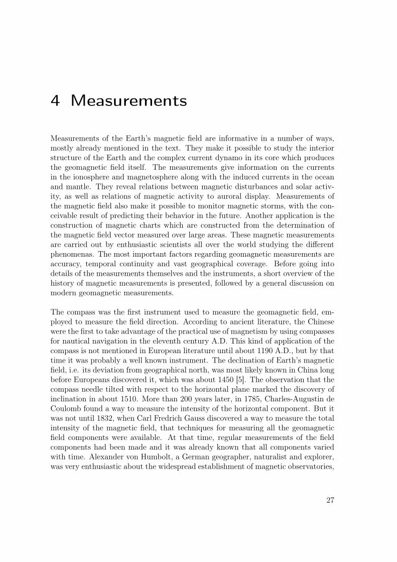
In addition to the magnetic observatories, which have well defined operation rules,magnetic field measurements are also carried out at magnetic repeat stations. Arepeat station is where the magnetic field is measured repeatedly every few years(ideally 2 years) [13]. Repeat stations are established with the aim of constructinga local map of the field or to get a better geographical coverage of magnetic fielddata. Most often they operate in connection with temporary research programs andonly in use for a short time in comparison with the magnetic observatories. Figure4.1 shows how repeat stations have been distributed over the world since 1900. Ingeneral, the same type of instruments are used at repeat stations and magnetic ob-servatories. While repeat stations do improve the global coverage of geomagneticdata, a true global coverage demands the establishment of automatic observatories.Currently, there are no automatic observatories that reach the standards which atypical magnetic observatory fulfills. Such observatories would lead to great im-provement in the field of geomagnetism. The magnetic measurements stated aboveare all ground based and do not tell the whole story. The magnetic field vectors canalso be obtained by magnetic instruments in space, using orbiting satellites. Themain difference between satellite and ground based magnetic measurements is thatthe former gives a global coverage with only one instrument while the latter needshundreds. However, only ground based measurements will be described here.

28

4.1 Geomagnetic Observatories

Figure 4.1: The worldwide distribution of repeat stations since 1900 [13].


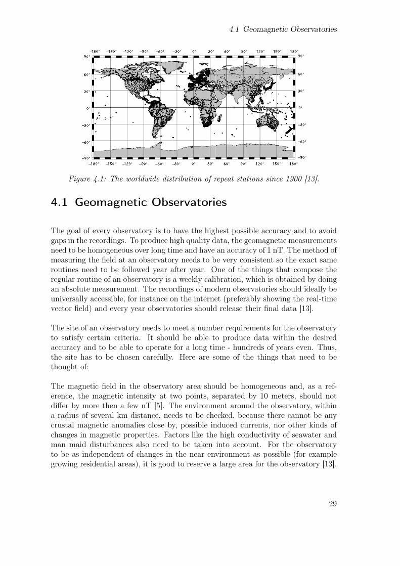
The goal of every observatory is to have the highest possible accuracy and to avoidgaps in the recordings. To produce high quality data, the geomagnetic measurementsneed to be homogeneous over long time and have an accuracy of 1 nT. The method ofmeasuring the field at an observatory needs to be very consistent so the exact sameroutines need to be followed year after year. One of the things that compose theregular routine of an observatory is a weekly calibration, which is obtained by doingan absolute measurement. The recordings of modern observatories should ideally beuniversally accessible, for instance on the internet (preferably showing the real-timevector field) and every year observatories should release their final data [13].

The site of an observatory needs to meet a number requirements for the observatoryto satisfy certain criteria. It should be able to produce data within the desiredaccuracy and to be able to operate for a long time - hundreds of years even. Thus,the site has to be chosen carefully. Here are some of the things that need to bethought of:

The magnetic field in the observatory area should be homogeneous and, as a ref-erence, the magnetic intensity at two points, separated by 10 meters, should notdiffer by more then a few nT [5]. The environment around the observatory, withina radius of several km distance, needs to be checked, because there cannot be anycrustal magnetic anomalies close by, possible induced currents, nor other kinds ofchanges in magnetic properties. Factors like the high conductivity of seawater andman maid disturbances also need to be taken into account. For the observatoryto be as independent of changes in the near environment as possible (for examplegrowing residential areas), it is good to reserve a large area for the observatory [13].

29

4 Measurements

Magnetic observatories can be a part of a larger research complex, operating at thesame location, or it can consist of only the basics needed for the magnetic fieldmeasurements. A typical magnetic observatory consists of five separate buildingsor huts: The main building, a variation house, an absolute house, an electricalhut and a proton magnetometer house. The distance from the electricity hut tothe sensors (located in the variation and absolute house) should not be less than15 m for the sensors not to be disturbed by it. Variometers are designed to beextremely sensitive so the material in the buildings housing them has to be non-magnetic. The variometers are placed on very stable pillars. In case local conditionsmake the construction of stable pillars difficult, other solutions are available, suchas suspended sensors (which are quite common), or the recording the tilt. As anexample of the importance of stable variometers, a shift of only one arcsecond is cancause a 0.24 nT change in a field of 50, 000 nT [13].

The temperature dependence of fluxgate variometers is 1 nT/◦C so the temperaturein the room (or box) where the variometer is placed, has to be very stable [5].The temperature should be determined with an accuracy greater than 0.5 ◦C butit is common practice to change the temperature twice a year following the averagetemperature outside. The variation room is just a shelter for the variometer becausenowadays they hardly need any service after instillation. Before, with the olderinstruments, they had to be visited on a daily basis.

In the the absolute house, only one non-magnetic pillar is needed and its stability isnot as important as for the variometers [5]. An azimuth mark (a sighting mark withknown azimuth), at a minimum distance of 100 m from the absolute house, needsto be in a line of sight from the pillar (seen out of a window), and the geographicaldirection of the mark has to be known. It is important for the instrument to havean accurate position on the pillar so there should be fixed slots for the instrumentto be placed in. Displacements of the instruments to the sides causes an errorin the declination.1 The further away the mark is located, the less sensitive themeasurement becomes of the displacement. The proton precession house only needsto contain a pillar and the main building can store data loggers, computers, clocksand other devices. An uninterrupted power supply is very important, since the aimis to operate the observatory continuously without any gaps in the recordings. Toavoid gaps, all systems should be supported by backup batteries in case of a powerfailure and run secondary systems in case of equipment failure. The secondarysystems are often older systems that have been replaced. To be able to use thedata from the secondary system, the recordings of the two types of systems shouldbe compared at regular intervals [5]. To get an idea about the layout of a typicalobservatory, an overview of Leirvogur observatory is shown in figures 4.2 and 4.3.

1Assuming the azimuth mark to be at a distance of 100 m distance, then a displacement of 1 cmof the instrument makes a change of 0.3 arcminutes in declination [5].

30


Figure 4.2: The layout of Leirvogur magnetic observatory [21].

Figure 4.3: Photograph of Leirvogur magnetic observatory, taken by Þorsteinn Sæ-mundsson. The picture is taken from the house Nýbær in figure 4.2, and thehouses in the picture are (from left) Móðabær, Flosabær, Miðbær and Vesturbær[22].

All objects close to the magnetometers need to be specially tested to make sure that

31

4 Measurements

they are non-magnetic. In the variometer room, the magnetic field from an object,at a distance of 0.5 from the sensor, should be less then 1 nT [5]. Where the absolutemeasurements are performed, the sensitivity of the measurement is even higher.

The standards for geomagnetic observatories are decided by INTERMAGNET. IN-TERMAGNET is a global network of magnetic observatories which advocates mag-netic observatory to produce high-quality data, and makes geomagnetic recordingseasily accessible on the internet. For an observatory to be a part of this network ithas to produce 1-minute data and fulfill other standard requirements set by INTER-MAGNET. All data produced within this international organization are thoroughlychecked by a team of experts before being published [13]. The number of partic-ipating observatories is constantly increasing, and in January 2010, 110 magneticobservatories worldwide were taking part [13]. The distribution of the observatoriesis shown in figure 4.4, where one can see vast areas without any observatories. Thisis a drawback which INTERMAGNET wants to improve, so they are always encour-aging more observatories to participate in the project. Recently, INTERMAGNEThas encouraged observatories to upgrade their data products to perform 1 Hz data(1 second data) and to constantly correct their data acquisition with a temporarybaseline [13]. This is done to meet the modern needs of the scientific society.

Figure 4.4: Global distribution of geomagnetic observatories that particpated in IN-TERMAGNET as of January 2010 (dots). The circles show the recently estab-lished observatories located in remote areas. [13].

4.2 Magnetometers

The role of a magnetic observatory is to continuously measure and report the ge-omagnetic field vector. The instruments used for measuring the field vector aretypically a triaxial fluxgate variometer (here referred to as a variometer), a fluxgate

32

4.2 Magnetometers

theodolite and a proton precession magnetometer (hereafter a proton magnetome-ter). The magnetometers are located at different places at the observatory site,but the final data, reported from a magnetic observatory, are always relative to oneparticular point. This means that all recordings, obtained from the magnetome-ters, need to be shifted to that particular reference point, which is often where theabsolute measurement is carried out.

The triaxial fluxgate variometer is an instrument that continuously records threevector components of the magnetic field (X, Y and Z) and thus yields the totalfield vector. The proton magnetometer also operates continuously but he only mea-sures the total intensity of the magnetic field vector. The total intensity values,obtained from the variometer and proton magnetometer, are constantly being com-pared because a change in the difference between them could mean a problem inone of the instruments.2 Finally, the fluxgate theodolite is used, together with theproton magnetometer, for a weekly calibration of the variometers. The fluxgatetheodolite measurement, which is done manually, reveals the declination and incli-nation of the geomagnetic field vector, and simultaneous measurements, performedby the proton magnetometer, give the total intensity of the field. By combining theresults from the two instruments, an absolute value of the geomagnetic field vectoris obtained. This procedure is therefore called an absolute measurement.

The variometer is calibrated by simultaneously comparing the components of thetotal geomagnetic field vector, obtained from the absolute measurement to that fromthe fluxgate variometer recordings. The differences between the vector componentsare referred to as baseline values for the variometer, where one baseline value isobtained for each component of the field [13]. The final data, reported from the ob-servatory, have the baseline values added to the values recorded by the variometer[5]. The reason why the absolute measurement needs to be performed on such aregular basis, is to correct for possible pillar instability due to tilting or rotation,temperature variation or drift of the instrument due to ageing [13]. This means, thateach week a new baseline value is obtained for each of the three field components.The values are usually plotted as a function of time, and a line fitted through thepoints is called a baseline. The quality of an observatory data is directly connectedto the homogeneity of the baseline. A continuously changing baseline indicates avariometer drift or other kind of instrumental instability, which of course is a badthing. However, a clear step in the baseline may indicate some kind of an event,for instance a rotation of the variometer (done intentionally for it to be directed to-wards magnetic north), or the changing of the room temperature to follow the meanoutdoor temperature. Figure 4.5 shows examples of the baseline values of Z, H andD components, and the adopted baselines, for the year 2010 in Leirvogur magneticobservatory. No obvious change in the baseline values can be observed, except forthe two large steps, which are associated with the changing of the temperature in

2The total intensity, F , measured by the fluxgate variometer is obtained by F =√X2 + Y 2 + Z2.

33

4 Measurements

the variometer house. Finally, it is worth mentioning the importance of all clocksconnected to the different instruments showing the exact same time, to one secondaccuracy. This is also required by the simultaneous measurements mentioned earlier,where the values from different instruments are compared at a certain time.

Figure 4.5: The adopted baselines at Leirvogur magnetic observatory in 2010 [21].

4.2.1 Fluxgate Magnetometers

There are various types of fluxgate magnetometers available and they are all basedon one or more fluxgate sensors. The principle of a fluxgate sensor is that itsoutput is proportional to the component of the external field in the direction of thesensors axis [20]. Now, the focus here will be on the application of the instrumentsand not on how they work, so the following simplified explanation of the fluxgatesensor will have to suffice. The basic fluxgate sensor consists of a core made of softmagnetic material, which should be easily saturable and have high permeability.

34

4.2 Magnetometers

The core has two coil windings around it, the excitation coil and the pick-up coil[1].3 Figure 4.6 show an example of a fluxgate sensor. If the excitation coil carriesan alternating current, with the frequency f , a magnetic field within the core willbe induced [5]. This causes the magnet to saturate and unsaturate, back and forth,whereas its magnetization follows the hysteresis curve of the material. If there is noexternal field, the induced signal in the pick-up coil will have the same frequencyas the excitation current. However, in the case of an external field, like the Earth’smagnetic field, the pick-up coil will measure a signal of other harmonics, additionalto those with the frequency f . The amplitude of these secondary harmonics, causedby the external field, is proportional to the intensity of the external field’s componentalong the sensor [5]. Thus, the signal in the pick-up coil yields the intensity of themagnetic field component aligned with the sensor.

Figure 4.6: Fluxgate sensor consists of a soft magnetic core and two coil windingsaround it; the excitation and pick-up coil [5].

The instruments at modern magnetic observatories, based on fluxgate sensors, arethe triaxial fluxgate variometer and the fluxgate theodolite. The triaxial fluxgatevariometer consists of three orthogonal fluxgate sensors, mounted in a marble cube,where two lie in the horizontal plane and one in the vertical. There are two typesof variometers available, one where the marble is suspended and one where it isnot. By suspending the sensors, the instrument will show much smaller drift. Thedifference in drift between the two types can reach 100 nT per year [2]. A suspendedfluxgate variometer is shown in figure 4.7, where the cube is suspended in two crossedphosphor-bronze strips [2]. The instrument is usually oriented in such a way thatone of the horizontal sensors is directed towards the geomagnetic north and thevertical sensor is aligned with the Z-component [13]. The instrument is connectedto digital data logger equipment where the signal from each sensor is converted andmodified to give the total intensity of each field component, in units of nT [21]. The

3A soft magnetic material has the ability to get magnetized but does not stay magnetized likepermanent magnets.

35

4 Measurements

Figure 4.7: Suspended triaxial fluxgate magnetometer. The fluxgate sensors (a) aremounted in a marble cube (b) and suspended with phosphor-bronze band (c) [13].

final data is obtained by adding the baseline values to the field components, aftercorrecting for possible sensor misalignments.

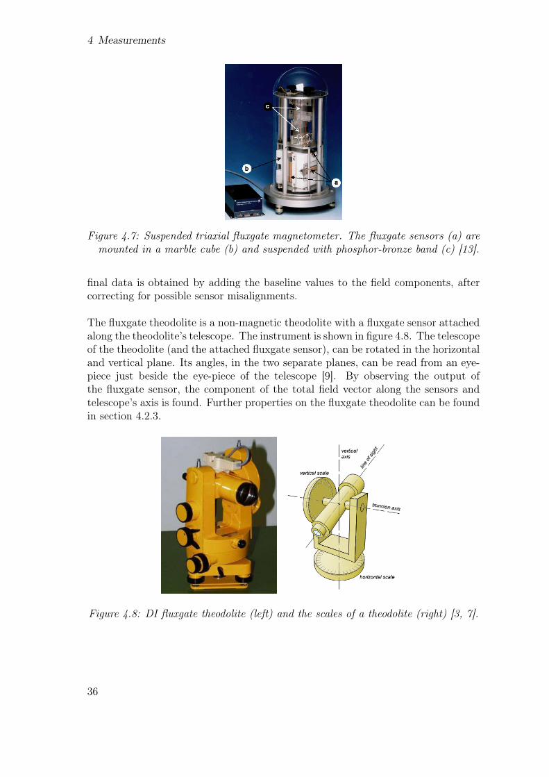
The fluxgate theodolite is a non-magnetic theodolite with a fluxgate sensor attachedalong the theodolite’s telescope. The instrument is shown in figure 4.8. The telescopeof the theodolite (and the attached fluxgate sensor), can be rotated in the horizontaland vertical plane. Its angles, in the two separate planes, can be read from an eye-piece just beside the eye-piece of the telescope [9]. By observing the output ofthe fluxgate sensor, the component of the total field vector along the sensors andtelescope’s axis is found. Further properties on the fluxgate theodolite can be foundin section 4.2.3.

Figure 4.8: DI fluxgate theodolite (left) and the scales of a theodolite (right) [3, 7].

36

4.2 Magnetometers

4.2.2 Proton Precession Magnetometer

Proton precession magnetometers are absolute instruments that measure the totalintensity in the magnetic field. The proton’s spin (its intrinsic angular momentum)tends to align with the external magnetic field, and the technique of these magne-tometers is based on the precession frequency of the proton’s angular momentum,L, around an external magnetic field B. The angular frequency of the precessionis given by ω = µB, and is called the Larmor frequency. The constant µ is thegyromagnetic ratio which depends on a particle’s charge and mass only, and B isthe magnitude of the external field, B = |B|. The gyromagnetic ratio for protonsis known with high accuracy, so if the precession frequency of L around B can bemeasured, the total intensity of the external field can be calculated. A proton mag-netometer consists of a bottle filled with proton rich fluid, like alcohol or water, anda coil system wounded around it. A direct current running through the coil inducesa magnetic field in the fluid which polarizes the protons in the direction of the field,causing a net magnetization [1]. When the artificial field is turned off, the proton’sangular momentum vector will start precessing around the Earth’s magnetic fieldwith the Larmor frequency, proportional to the strength of the field. The protons’precession induces an AC voltage of the same frequency, and by dividing the fre-quency with the gyromagnetic ratio, the strength of the Earth’s magnetic field canbe deduced [13, 1]. The electronics have to be able to measure a frequency withan accuracy of 10−5. To give an example of the precession frequency, protons in a45, 000 nT field will precess with frequency close to 2 kHz [1].

4.2.3 Absolute Measurements

Once a week, an absolute measurement is carried out at magnetic observatories,according to a fixed routine. The inclination and declination of the geomagneticfield is found by the use of a DI-flux, which is the fluxgate theodolite shown in fig-ure 4.8, while the simultaneous total intensity of the field is obtained by a protonmagnetometer located in the area. For the absolute value of the field vector to beobtained, the value of the field’s intensity needs to be shifted from the location ofthe proton magnetometer to the absolute pillar for it to represent the same vec-tor as the inclination and declination. This means, e.g. that before or after theI and D measurement, the difference in the total field intensity, between the twolocations, needs to be evaluated. That is done by placing another proton magne-tometer on the absolute pillar and comparing the field intensities obtained by thetwo magnetometers simultaneously.

The determination of the inclination and declination is based on finding the positionsof the sensor, aligned with the telescope, where the output is close to zero. Since

37

4 Measurements

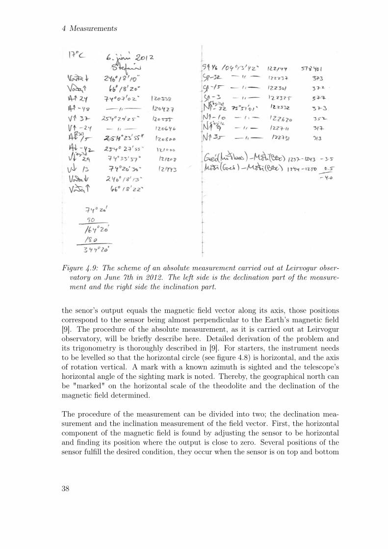
Figure 4.9: The scheme of an absolute measurement carried out at Leirvogur obser-vatory on June 7th in 2012. The left side is the declination part of the measure-ment and the right side the inclination part.

the senor’s output equals the magnetic field vector along its axis, those positionscorrespond to the sensor being almost perpendicular to the Earth’s magnetic field[9]. The procedure of the absolute measurement, as it is carried out at Leirvogurobservatory, will be briefly describe here. Detailed derivation of the problem andits trigonometry is thoroughly described in [9]. For starters, the instrument needsto be levelled so that the horizontal circle (see figure 4.8) is horizontal, and the axisof rotation vertical. A mark with a known azimuth is sighted and the telescope’shorizontal angle of the sighting mark is noted. Thereby, the geographical north canbe "marked" on the horizontal scale of the theodolite and the declination of themagnetic field determined.

The procedure of the measurement can be divided into two; the declination mea-surement and the inclination measurement of the field vector. First, the horizontalcomponent of the magnetic field is found by adjusting the sensor to be horizontaland finding its position where the output is close to zero. Several positions of thesensor fulfill the desired condition, they occur when the sensor is on top and bottom

38

4.2 Magnetometers

of the telescope, and the telescope is directed approximately East and then West.For each of the positions, the horizontal angle and the output of the sensor is noted.From this information, the declination of the geomagnetic field vector can be found.

Figure 4.9 shows the scheme of an absolute measurements performed at Leirvogurobservatory, where A, V, N, S correspond to East, West, North and South, and thesigns ↓ and ↑ refer to the sensor being on top (↑) or under (↓) the telescope. Theleft side of the figure corresponds the declination measurement described above andthe right side of the figure corresponds to the following inclination procedure. Notethat the different positions of the sensor cancel the effect of the possible differencebetween the alignment of the axis of the telescope and the sensor’s axis [9].

In the latter part of the measurement, the inclination of the magnetic field is found byaligning the sensor with the magnetic meridian, whereas the magnetic meridian canbe found from the earlier declination measurement. When in the magnetic meridian,the sensor is rotated about the horizontal axis, again placed at the position wherethe sensor’s output is close to zero, where the vertical angle and the output is noted.As can be seen in figure 4.9, four measurements are done with the sensor on top andtelescope facing South and then other four where the telescope faces North. Thesimultaneous total intensity of the field, measured from the proton magnetometeris also noted for each measurement. At the bottom of the right side of figure 4.9,one can see that the difference in the total intensity of the magnetic field vectorbetween the location of the absolute pillar and the proton magnetometer has beenfound. From these series of measurements, the inclination, declination and the totalintensity of the geomagnetic field vector at the absolute pillar can be deduced.

39

5 Summary and Conclusions

The magnetic field observed at the surface of Earth is a superposition of magneticfields generated by different sources. The most dominant source by far, is the com-plex current system in the Earth’s highly conducting and liquid outer core. TheEarth’s magnetic field is a vector field so three components are needed to fullydescribe the field at a given point, usually the horizontal component, vertical com-ponent and the declination of the vector are specified. Spherical harmonics canbe used to describe the magnetic field on the Earth’s surface, and are commonlyapplied in the construction of global magnetic charts. Direct measurements of thegeomagnetic field and the study of paleaomagnetism, reveal that the geomagneticfield changes with time. Long term variations, also called secular variation, whichare on the scale of several years to a million years, are due to the dynamics withinthe Earth’s interior - those producing the main field. Variations on a shorter timescale are due to currents in the magnetosphere and ionosphere, which in turn causeinduced currents in the Earth’s crust and oceans. These magneto- and ionosphericcurrents originate from the changing shape of the Earth’s magnetosphere, which isa response to the incoming the solar wind.

Continuous measurements of the Earth’s magnetic field are performed by magneticobservatories worldwide, which have the combined goal of recording magnetic datawith the highest possible accuracy and to avoid gaps in the recordings. The obser-vatories communicate with each other and exchange data, together making a globalnetwork of magnetic observatories. The main instruments of a modern geomagneticobservatory are the triaxial fluxgate variomter, the fluxgate thodolite and the protonprecession magnetometer. The field components are continuously and automaticallymeasured by the triaxial fluxgate variometer but a weekly calibration needs to beperformed by hand, using the fluxgate theodolite and the proton precession magne-tometer.

If the reader is interested, the field of space weather and satellite based magnetome-ters could be suitable for further reading. There are many exciting ongoing, andforthcoming missions, with the focus on examining the Earth’s magnetosphere andits interaction with the solar wind. That is something definitely worth following.It is good to keep in mind that each chapter is only a summarization of the maindetails of the corresponding subject. For further reading on the different subjects,the cited books and articles are recommended.

41

Bibliography

[1] Auster, H.U. (2008). How to measure Earth’s magnetic field Physics Today,61(2). 76-77.

[2] Danish Meteorological Institute Fluxgate Magnetometer, Suspended Verson,Model FGE version K, Manual. Copenhagen: DMI, 2006.

[3] "Fluxgate Declinometer/Inclinometer Instrument." 5 Jun. 2012. http://www.mingeo.com/products/theodolit.htm

[4] Fox, K.C. "Storms From the Sun." 5 Jun. 2012. http://www.nasa.gov/mission_pages/sunearth/news/storms-on-sun.html

[5] Jankowski, J. and Sucksdorff, C. Guide for Magnetic Measurements and Ob-servatory Practice. Warszawa: International Association of Geomagnetism andAeronomy, 1996.

[6] Karttunen, H. et al. Fundamental Astronomy. Springer, 2007.[7] Kunkel, P. "Theodolite Error." 5 Jun. 2012. http://whistleralley.com/

surveying/theoerror/[8] Lanza, R. and Meloni, A. The Earth’s Magnetism - An Introduction for Geol-

ogists. Würzburg: Springer, 2006.[9] Laruidsen, E.K. Experiences with the DI-fluxgate Magnetometer Inclusive The-

ory of the Instrument and Comparison with Other Methods. Copenhagen: Dan-ish Meteorological institute, 1985.

[10] Love, J.J. (2008). Magnetic Monitoring of Earth and Space Physics Today,61(2). 31-37.

[11] Magnetic North, Geomagnetic and Magnetic Poles. 5 Jun. 2012. http://wdc.kugi.kyoto-u.ac.jp/poles/polesexp.html

[12] "Magnetosphere rendition.jpg" 5 Jun. 2012. http://en.wikipedia.org/wiki/File:Magnetosphere_rendition.jpg

[13] Matzka, J., Chulliat, A., Mandea, M., Finlay, C.C. and Qamili, E. GeomagneticObservations for Main Field Studies: From Ground to Space. Publised online:Springer, 2010

[14] McPherron, R.L. "Geomagnetic field." 5 Jun. 2012. http://www.britannica.com/EBchecked/topic/229754/geomagnetic-field/

[15] Merrill, R.T. and McElhinny, M.W. The Earth’s Magnetic Field - Its History,Origin and Planetary Perspective. Orlando: Academic Press, Inc., 1983.

[16] Mullan, D.J. Physics of the Sun. Florida: Chapman and Hall/CRC, 2010.[17] National Gephysical Data Center. 5 Jun. 2012. http://www.ngdc.noaa.gov/

wist/magfield.jsp[18] Nave, R. "Magnetic Field of the Earth." 5 Jun. 2012. http://hyperphysics.

phy-astr.gsu.edu/hbase/magnetic/magearth.html[19] Phillips, T. "Earth’s Inconstant Magnetic Field." 5 Jun. 2012. http://www.

nasa.gov/vision/earth/lookingatearth/29dec_magneticfield.html[20] Primdahl, F. The Fluxgate Magnetometer. Copenhagen: Danish Meteorological

43

http://www.mingeo.com/products/theodolit.htm

http://www.mingeo.com/products/theodolit.htm

http://www.nasa.gov/mission_pages/sunearth/news/storms-on-sun.html

http://www.nasa.gov/mission_pages/sunearth/news/storms-on-sun.html

http://whistleralley.com/surveying/theoerror/

http://whistleralley.com/surveying/theoerror/

http://wdc.kugi.kyoto-u.ac.jp/poles/polesexp.html

http://wdc.kugi.kyoto-u.ac.jp/poles/polesexp.html

http://en.wikipedia.org/wiki/File:Magnetosphere_rendition.jpg

http://en.wikipedia.org/wiki/File:Magnetosphere_rendition.jpg

http://www.britannica.com/EBchecked/topic/229754/geomagnetic-field/

http://www.britannica.com/EBchecked/topic/229754/geomagnetic-field/

http://www.ngdc.noaa.gov/wist/magfield.jsp

http://www.ngdc.noaa.gov/wist/magfield.jsp

http://hyperphysics.phy-astr.gsu.edu/hbase/magnetic/magearth.html

http://hyperphysics.phy-astr.gsu.edu/hbase/magnetic/magearth.html

http://www.nasa.gov/vision/earth/lookingatearth/29dec_magneticfield.html

http://www.nasa.gov/vision/earth/lookingatearth/29dec_magneticfield.html

BIBLIOGRAPHY

institute, 1979.[21] Science Institute - University of Iceland. Leirvogur, Magnetic results 2010.

Reykjavík, 2010.[22] Segulmælingastöðin í Leirvogi. 5 Jun. 2012. http://www.raunvis.hi.is/

~halo/leirvogur.html[23] "Sun Storm: A Coronal Mass Ejection." 5 Jun. 2012. http://www.astronet.

ru/db/xware/msg/1162723[24] Steigerwald, B. "Sun Often "Tears Out A Wall" In Earth’s Solar Storm Shield."

5 Jun. 2012. http://www.nasa.gov/mission_pages/themis/news/themis_leaky_shield.html

[25] Sæmundsson, Þ. "Árstíðasveiflan í segultruflunum og norðurljósum." 5 Jun.2012. http://www.internet.is/halo/halfsars.html

44

http://www.raunvis.hi.is/~halo/leirvogur.html

http://www.raunvis.hi.is/~halo/leirvogur.html

http://www.astronet.ru/db/xware/msg/1162723

http://www.astronet.ru/db/xware/msg/1162723

http://www.nasa.gov/mission_pages/themis/news/themis_leaky_shield.html

http://www.nasa.gov/mission_pages/themis/news/themis_leaky_shield.html

http://www.internet.is/halo/halfsars.html

the earth’s magnetic field - heim | skemman ·...

Documents