Yale University

The Effect of Supermarket Entrance on Nearby Residential Property Values in the United States

from 1997 to 2015

William Van Fossen Economics 491-492: The Senior Essay

Advisor: Jason Abaluck, Yale School of Management April 3rd, 2017

1

Table of Contents

1. Introduction………………………………2

2. Objective…………………………………3

3. Literature Review………………………..4

4. Data Sources……………………………..12

5. Methodology……………………………..15

6. Results/Discussion/Limitations………….30

7. Concluding Remarks…………………….34

VanFossen

2

1. Introduction

The topic and question of how supermarkets affect the dynamic of a neighborhood has

been analyzed in numerous studies in the past and appeared frequently throughout popular media

outlets. In the United Kingdom, headlines were made when Lloyd’s Bank released a study

coining the term “The Waitrose Effect”, citing the value that popular supermarket brands add to

homes within certain proximity. The name, The Waitrose Effect, was decided on due to the

estimation that Waitrose served as the greatest value-add towards residential property values out

of all supermarket chains in the U.K. (Lloyd’s Bank 2016). Major media outlets in the United

States such as the New York Times and The Atlantic have both published several articles

discussing the gentrifying effect supermarkets can have in neighborhoods following their

opening. In the New York Times’ discussion of the Bloomberg administration's efforts to spread

healthy eating across the city, the gentrification that is said to occur throughout the boroughs of

the city (as a result from the supermarkets) is a major talking point (Cardwell 2003). The

Atlantic explores the protest in Portland, Oregon that occurred against the construction of a

Trader Joe’s in a vacant lot in an effort to avoid the gentrifying aftermath in its 2016 article,

“When a Grocery Store Means Gentrification” (Smith 2016). Thus, this interest in the

supermarket and how it affects the dynamic of a neighborhood is one that has made its way into

both countless studies and into the popular media.

In order to study the dynamic that exists between the two entities of the supermarket and

the neighborhood, residential property values are used in this report. Residential property values

provide a quantifiable metric that allows the effect an introduction of a supermarket has on a

neighborhood to be determined using hedonic estimation techniques. The data pertaining to

these residential property values comes from the online real estate marketplace, Zillow’s

3

research platform at the neighborhood level, the smallest region unit that the database provides.

The data pertaining to supermarkets was obtained from the database, Reference USA, a division

of InfoGroup. The spatial analysis performed to determine the entrance and exit of supermarkets

within specific boundaries of neighborhoods was done using computer mapping software,

ArcGIS. The data produced using ArcGIS was then used towards completing the hedonic

estimation. These regressions were performed using data analysis and statistical software,

STATA, to produce the final results of this report.

Following the introduction of this paper the main objective of the research will be

discussed. After the objectives and goals are described the paper will go through a review of

literature that has accomplished similar research into determining the effect that supermarkets or

other entities have on property values within certain proximity. Following this review, the paper

will explain the data collection process and the data sources that were used to achieve the results

of this study. Subsequently, the methodology that was used and the different tools used to

perform the research will be described. The paper will then walk through the results that were

obtained from the chosen data and methodology. In conclusion, the concluding section of the

paper will discuss the entirety of the report and include final remarks.

2. Objective

The objective of the research described in this paper is to determine the effect the

introduction of a supermarket within a specified proximity to a neighborhood has on the

residential property values within that neighborhood. This effect will be examined at the radii of

one mile, three miles and five miles around neighborhoods throughout different parts of the

country. The main goal is to determine if and what premiums supermarkets are adding to homes

VanFossen

4

and how this changes when the distance between the home and the supermarkets changes. Thus,

this research attempts to determine the best estimate of the relationship between supermarket

entry and housing values using the change in housing value as a measuring instrument for this

dynamic.

3. Literature Review

As discussed in the introduction, the “value add” of supermarkets is something that has

been frequently studied and appeared both in many formal research papers and throughout many

popular media outlets across the country and the world. In many cases it has been looked at

more specifically through the lens of food deserts and gentrification. This analysis typically goes

far beyond just the quantitative analysis and includes the study of complex social issues as well.

Other papers take a strictly economic and quantitative approach and focus on a more typical area

without food access problems just to determine what kind of a premium a supermarket or other

entity is contributing to the value of a home. In either case, both types of research are attempting

to answer the fundamental question of how a supermarket or other entity affects a neighborhood

in one way or another.

Lloyd’s Bank performed one of the more popular studies addressing this topic. The bank

conducted research to determine how much of an effect a supermarket in near proximity to

homes has on the residential property values. The study was conducted in an effort to see if the

“Waitrose Effect” was in fact true, and actually causing homes in its area to be valued at a

premium. The banking group did not only analyze homes around Waitroses, but also many other

supermarket chains in the UK such as Sainsbury’s, Tesco, Aldi and Lidl. The study was

5

conducted using data from “CACI Ltd” for supermarket locations, and average housing values

for 12 months leading up to March 2016 obtained from the Land Registry (Lloyds Bank 2016).

To find the results, the average prices of homes in a town within the same postal district as the

supermarket were compared to the average price of the homes in the rest of the town outside of

that area (Lloyds Bank 2016).

On average it was found in the study found that, “living close to a well-known

supermarket chain can add an average of £22,000 to the value of your home” (Lloyds Bank

2016). This number was determined using the premiums calculated from all of the different

types of supermarkets studied, from the high-end end of the spectrum to the low-end portion.

£22,000 is certainly not a negligible number when evaluating property values of single family

residences. The high-end stores that were found to add the most value to nearby homes were

Waitrose and Sainsbury’s. The two chains were found to add a premium of £38,666 and £27,939

respectively (Lloyds Bank 2016). Mike Songer, the Lloyds Bank Mortgage Director, was quoted

in the report saying, “Our figures show that the amount added to the value of your home can be

even greater if located next to a brand which is perceived as upmarket” (Lloyds Bank 2016).

Waitrose and Sainsbury’s are the epitome of such “upmarket” stores throughout the United

Kingdom. On the low-end side stores such as Lidl and Aldi added the smallest premium to

nearby homes, calculated at £3,926 and £1,333 respectively (Lloyds Bank 2016). These two

brands are seen as the opposite of “upmarket” in the U.K. and rather as more of budget grocery

stores.

One drawback in this study is that these higher property values could be caused by a

multitude of reasons that do not seem to have been controlled for. Supermarkets in England tend

to be in the town center and homes in the town center tend to be more expensive as they are close

VanFossen

6

to a number of amenities. This is why it could be important to look at how property values are

changing after the introduction of a supermarket, or after something changes in relationship to

food access. This research also differs from the research that is the main focus of this paper

because its focus was on supermarkets and property values in the United Kingdom. The focus of

this paper will be on supermarkets from across the United States. There is the potential for

supermarkets to be valued quite differently between the two nations.

Mingche Li and James Brown of the Land Economy Department at the University of

Wisconsin-Madison conducted another similar research project. The report was titled, “Micro-

Neighborhood Externalities and Hedonic Housing Prices.” This study looked at the effect that

micro-neighborhood externalities have on housing prices. The main finding was that proximity

to non-residential land uses can have positive externalities on housing prices by acting to

increase accessibility, but on the other hand can also have a negative externality by increasing

negative externalities such as “diseconomies” (Li 1980). These diseconomies are stated to be,

“congestion, pollution and unsightliness” (Li 1980). The study looks at three main micro-

neighborhood variables that produce these externalities. These variables are stated as, “aesthetic

attributes, pollution levels and proximity” (Li 1980). The idea presented in the paper is that the

introduction of a new non-residential land use would surely alter these three variables and

subsequently the residential property values.

The proximity variable is most relevant to the research that will be discussed later in this

paper. In the paper by Li and Brown the proximity variable refers to the proximity of corner

grocery stores, neighborhood parks, schools, rivers, oceans or conservation lands. The corner

grocery stores are the most similar to what this paper will later discuss in regard to grocery stores

7

and supermarkets. The study makes a point that the proximity to these different non residential

land uses is usually seen as something that increases residential property values, but there can

also be externalities of congestion, noise and air pollution that would decrease the value of a

home (Li 1980). Hence, it is not clear exactly what the net effect will always be when a non-

residential land use property is located in proximity to a residential property based on the

findings in this study.

It is stated in the study that the data used for the residential property values comes from,

“a sample of 781 sales of single family homes in 15 suburban towns located in the southeast

sector of the Boston metropolitan area” (Li 1980). The sales data was taken from single-family

home transactions that occurred in these areas in the year of 1971 and had been recorded within

the multi-listing real estate database (Li 1980). Hedonic estimation was then completed using

these sales prices and several micro-neighborhood accessibility variables. One example of the

main results of this study was that, “The effect of noise pollution is to reduce sales price by an

average of $460 for each doubling of the perceived level of loudness” (Li 1980). Thus, this

describes the results of one of the factors, a commercial presence, and how it could potentially

have an affect on a nearby home.

The use of single-family home transactions allowed this study to obtain accurate pricing

based on supply and demand of the home that was being sold. A different method of gathering

the property values will be used in the research discussed in this paper, provided by Zillow. Li

and Brown also only looked at the effect nonresidential land uses were having on property values

in the Boston area, whereas in the research discussed in this paper, supermarkets and property

values will be analyzed in groups of neighborhoods from all across the United States.

VanFossen

8

In addition, other research has been carried out in order to use hedonic estimation to

determine the effects other entities have on residential property values. An example of one of

such studies is titled, “Estimating the Effects of High Rise Office Buildings on Residential

Property Values” by Thomas G. Thibodeau in 1990. As the title suggests, this study uses

hedonic estimation to approximate the effect a high-rise office building has on residential

property values in its proximity. A small residential area in North Dallas is used as the sample

area and the Lennox Center, which was constructed in 1980 in North Dallas, is the main focus of

the study as the independent variable (Thibodeau 1990). The data used in the hedonic estimation

to account for the residential property values was taken from the sales data from 1977 to 1988

and the associated housing characteristics (Thibodeau 1990). The characteristics of the

properties used were stated to be, “characteristics of the lot, characteristics of the improvement,

neighborhood amenities, proximity variables, and land use regulations” (Thibodeau 1990). In

the estimation that followed using this data the study accounted for both positive and negative

externalities that resulted from the construction of the tower. The negative externalities were

subtracted from the positive externalities to find the net effect of the office building. As a result,

this study found that the office building had a net positive effect on the residential property

values of about 1 percent (Thibodeau 1990).

The research discussed in this paper will differ from the research discussed in

Thibodeau’s paper for several reasons. First and foremost, the research in this paper focuses on

the effect grocery stores have rather than a high-rise office building. The reason attention is

drawn to Thibodeau’s paper is because of the similar hedonic technique he uses in his analysis.

Even though office buildings are used, the study is still very relatable to one that uses

supermarkets or grocery stores instead. Another way this study differs from the focus of this

9

paper is because only one single neighborhood of property values and one high-rise office

building are used in an effort to find a general effect. In the study that is the focus of this paper,

many neighborhoods and many supermarkets are used to determine the effect that the

supermarket has on residential property values, rather than just one of each. This allows for a

more accurate representation of what happens in a typical scenario.

Yet another example of a study using this method of hedonic estimation is titled, “Effects

of Transportation Accessibility on Residential Property Values” by L. Miguel Martinez and Jose

Manuel Viegas. This 2009 study focused on the Lisbon, Portugal metropolitan area and

determined how a location's proximity and accessibility to transportation services affected the

residential property values in the area. The reason that this study was carried out was stated as,

“to assess whether public investment in transportation can modify residential property values”

(Martinez 2009). Three different types of transportation systems are used in this study; metro,

rail and road (Martinez 2009). These forms of transportation play the role of the independent

variable in this hedonic estimation. The residential property values are of course the dependent

variable.

The data in this study for the residential property values comes from the online realtor’s,

“Imokapa Vector,” database of the 2007 cross sectional sales data (Martinez 2009). This

database contained details on, “the asking sale price, the structural attributes and the address”

(Martinez 2009). These three variables allow for the study’s hedonic estimation and also allow

for a spatial analysis using the location of the homes. The data for transportation services was

obtained using the Lisbon Mobility Plan 2004 and it was stated that, “local accessibility

indicators were calculated with the network distance to public transport entry points” (Martinez

VanFossen

10

2009). This was used in the hedonic estimation in two different ways. In one approach the

entrances to transportation services were recorded as being within a certain distance or not, and

in the other approach the entrances to transportation services were recorded on the basis of how

far they were located from the residential properties. In the first approach this means they were

recorded in a yes or no, or one or zero kind of fashion and in the second approach a range of

numbers could have been used to indicate distance. These different approaches were used to

obtain the answers to similar questions.

The results of this study showed different effects on property values ranging from

negative to positive for different transportation services (Martinez 2009). The methods used to

obtain these results do come with their limitations. One of such limitations is that the data for

the residential property values is associated with the asking price for the homes. The asking

price is not a reflection of the actual value of the home based on demand, but rather just what the

seller would like to receive for the home or perhaps thinks is realistic. If the study had been able

to use all sale prices this would have created a more accurate representation of actual equilibrium

prices being sold. This strategy also has its drawbacks as well though, being that it is difficult to

find as many actual sale prices, and sale prices could be skewed in a certain direction in a given

year. A combination of the two may have contributed to a better format for running the hedonic

estimation. In order to combat this problem, the data used in this paper was drawn from Zillow,

claiming to avoid these biases in their data collection.

Several conclusions can be drawn from the reviewed literature. One major conclusion is

that the expected results differ from study to study. In the study by Lloyds Bank examining the

Waitrose Effect, the results were largely what were expected from the outset. Being in close

11

proximity or within the same postal code as a supermarket increased residential property values,

and the observed increase was greater with the high-end stores and smaller with the low-end

stores (Lloyds Bank 2016). In the study looking at transportation, it may be commonly believed

that being close to a form of transportation would increase property values but in the study

conducted in Portugal, it was found that this effect could be both positive and negative on

housing values (Martinez 2009). Hence, the magnitude and direction in which an effect occurs is

not always equal to what intuition would suspect.

Another conclusion is that where the data is coming from and what type of data is being

used is very important to the results and quality of the study. In the study looking at the effect

that high-rise office buildings have on residential property values, the data collected was very

specific. There was a focus on one high-rise office building, The Lennox Center, and one

neighborhood in North Dallas (Thibodeau 1990). The study could have been more accurately

described by saying it analyzed the effect the Lennox Center had on residential property values

in its proximity, rather than high rise office buildings in general on residential property values.

In the study looking at the effect micro neighborhood externalities have on housing prices; single

home transaction data was used to account for the housing prices. It is important to note that this

type of data is not always the most accurate. For example, in a given year more expensive

homes could have been sold and less inexpensive homes could have been sold. This would

present a higher average home price in an area for a given time period than the actual average.

Thus, looking at the data and where it is from is very important to understanding the results of a

study.

VanFossen

12

4. Data Sources

The data used in this study came from two main sources. The dependent variable,

residential property values, was obtained from a public database provided by the online real

estate platform, Zillow. The independent/explanatory variables, or the factors that were believed

to have an effect on residential property values, were obtained from ReferenceUSA. Both

comprehensive datasets allowed for a regression to be run in order to determine the effect that

supermarkets have on residential property values.

4.1 Zillow Data

The residential property values dataset made publicly available by Zillow is known as the

ZHVI All Homes Time Series data set (Bruce 2014). ZHVI stands for the Zillow Home Value

Index. This data is offered at a series of different levels ranging from the smallest level of

neighborhood to zip code, city, county, metro area and finally to the largest level of state (Bruce

2014). Each level uses the same techniques to provide an average residential property value for

the area. The data sets also range in what type of residential units they are providing values for.

These categories of residential units consist of one to five bedroom homes, single-family homes,

condos/co-ops and all homes (Bruce 2014). The data set for this study used the “All Homes” for

the type of residential unit and the “Neighborhood” level for the scale at which the residential

unit was viewed. These were chosen because the “All Homes” provides the most possible data

for residential living units, thus helping to provide a more accurate portrayal of how supermarket

introduction would affect their values. The “Neighborhood” level was chosen because it was the

smallest scale at which the residential property values were observed, thus making it the most

sensitive level at which a supermarket's entrance could disrupt the property values. The smaller

13

the area that could be used resulted in a more precise look at the effect a single supermarket’s

entrance or exit would have. Thus, this is why the neighborhood and all homes dataset was

chosen for this research.

Zillow uses a system of “Zestimates”, which was developed in 2005 to estimate

residential property values in their datasets (Bruce 2014). The index Zillow created is based off

of these estimated sales prices of every home. The estimation error for each individual home

“Zestimate” is just as likely to be above the actual sales price as it is to be below (Bruce 2014).

This leads to what Zillow considers an accurate estimation when looking at a large group of

homes such as across a neighborhood.

Zillow states that what makes its index better compared to other property valuation

indexes are that other indexes only use the data of homes that actually sold in a region (Bruce

2014). Although this sounds as if it could be more accurate, Zillow makes the argument that

when an estimate is based on only the actual sales prices it may be common to run into some

biases. An example would be if during a certain time period a neighborhood experienced the

sale of more expensive homes and less inexpensive homes than normal, the average for home

prices in that neighborhood during that time period would be skewed as more expensive than

they really were. Zillow combats this bias by including estimates of all homes in their index and

not just the sale prices of homes. By doing this, their database is resistant to presenting a skewed

average of home values if there is a period where more expensive homes are sold than

inexpensive homes.

The Zillow estimations are conducted by running simulations using computers. The

programs developed perform these estimates based on “proprietary statistical and machine

learning models” (Bruce 2014). It is stated that these estimates take into account, “recent sale

VanFossen

14

prices and various home attributes” (Bruce 2014). These home attributes consist of metrics such

as, “physical facts about the home and land, prior sale transactions, tax assessment information

and geographic location” (Bruce 2014). The computer is able to learn patterns between the sales

transactions and the home attributes and as a result provides estimations for all homes whether

they were sold recently or not. The goal of this estimate is stated to be to give, “consumers

insight into the home value trends for homes that are not being sold out of foreclosure status”

(Bruce 2014). As a result, the database provides a representation of residential property values at

several different levels of organization.

4.2 ReferenceUSA Data

The independent variables in the study come from ReferenceUSA, a division of

InfoGroup that began collecting business data in 1972. The company collects information on

businesses and residences across the United States of America and is maintained and updated

daily. ReferenceUSA maintains its database by “continuously updating from more than 5,000

resources,” and these listings are verified and kept up to date by placing over 24 million phone

calls per year (“Reference USA – Data Quality” 2017). Another strategy used by the firm is

“web mining” or “deep web mining” (Lea 2017). This provides the company with a more

efficient way to extract data from a business’s website, by pulling out data such as store locations

(Lea 2017). This maintenance leads to the database adding 2 million new companies per year on

average which comes out to about 10,000 being added daily (Lea 2017). On the other hand, this

maintenance also leads to businesses being removed from the database, although they still

remain in the historical database. On average, just over 1,500 businesses are removed from the

database in a given hour (Lea 2017). The listing for each business includes many important

15

characteristics and statistics including, “company name and phone number, complete address,

key executive name, SIC codes, employee size, sales volume, business expenditures and much

more” (“Reference USA – Data Quality” 2017). The company states that the data compiled by

ReferenceUSA, “powers and verifies the world’s top search engines” and “serves 70 of the

Fortune 100 companies” (Lea 2017). This source of data is used both for research in the

academic world and research in the business world establishing itself as the top data source for

historical and current nationwide business records.

The main information taken from ReferenceUSA for this project was latitude and

longitude coordinates, which were crucial in executing the spatial analysis. Another important

component of Reference USA was the Primary NAICS code option that is used in filtering

through data. The NAICS code system refers to the “North American Classification System”

and the Primary NAICS means that the code is referring to the business’s primary purpose

("North American Industry Classification System." 2017). The ability to sort through businesses

classified by their primary purpose proved to be very useful in finding the right data. Thus, the

latitude and longitude coordinates and the NAICS codes provided by ReferenceUSA were

critical components of presenting the independent variables.

5. Methodology

5.1 Data Collection

Data collection from the sources summarized above was the first step towards finding the

results in regard to the effect of supermarket introduction on residential property values. The

data obtained from Zillow pertaining to residential property values ranged from 1996 to 2016 on

a monthly basis. These monthly data points were eventually consolidated into annual averages

VanFossen

16

later in the research. Along with the neighborhood level property values, Zillow also provided

the neighborhood crosswalks, also known as shapefiles, which allow the data to be presented in

mapping software. In total, 6,957 neighborhood shapefiles and their appropriate average

residential property values per month were downloaded and used in the research. The shapefile

data made it possible to perform spatial analysis, and the property value portion of the data made

it possible for the more quantitative aspects of the study to be executed.

Data was also obtained from ReferenceUSA to account for the supermarkets and

shopping centers across the country. The restrictions on data for the supermarkets was that it had

to be from 1997 to 2015 (upper and lower bounds of the accessible data), the Primary NAICS

code for the business had to be 445110 (Primary NAICS code for supermarkets and other

grocery stores), and the store needed to have over 50 employees. Beyond these few restrictions

the data for supermarkets was drawn from the entire United States. The last specification in

regard to the number of employees was set to make sure the supermarkets used in the study were

large enough to have a significant effect on the property values. This could have been achieved

with several different restrictions such as square footage of the store or annual revenue, but the

number of employees seemed most applicable to the regional effect the research was looking

most closely into. The most important characteristics of each downloaded supermarket were the

latitude and longitude coordinates and the archived year. The coordinates allowed for each

individual supermarket to be plotted on a map and the archived year allowed for the entry and

exit of markets to be examined by year. In total, the results of this query drawing data from

across the entire nation lead to 270,361 results.

The other portion of data obtained from ReferenceUSA was for shopping centers across

the country. Once again, this data for shopping centers ranged from 1997 to 2015, the time

17

restraints at which the download was subject to. The shopping centers were designated in the

ReferenceUSA dataset by the SIC code. There is no existing NAICS code for shopping centers,

so in this case the SIC system was used. This stands for Standard Industrial Classification and is

a very similar system to the NAICS codes described above. The SIC code for shopping centers

used in the query was 651201, the code for “Shopping Centers and Malls.” There was no

restriction on the number of employees for this variable as the assumption was made that all

shopping centers or malls would be at a minimum size large enough to represent the effect of

commercialization. Once again, the most important characteristics of each downloaded shopping

centers were the latitude and longitude coordinates and the archived year. The coordinates

allowed for each individual shopping center to be plotted on a map and the archived year allowed

for the entry and exit of centers by year to be included as well. In total, the results of this query

for shopping centers led to the download of 36,704 results.

5.2 Spatial Analysis

Following the retrieval of the data from Zillow and ReferenceUSA, the necessary portion

of the research devoted to spatial analysis began. The mapping software ArcGIS, more

specifically ArcMap, was used to put this data within a platform where it could be examined and

analyzed in a spatial environment. The constructed map consisted of a base layer of the United

States upon which the other layers of data were then added. Following the establishment of the

base layer, the polygons corresponding to each of the neighborhoods from Zillow were added to

the map. These neighborhoods by no means covered the entirety of the nation but were able to

provide analysis in many different regions of the country. FIGURE 1 displays the map with only

the base layer of the United States and the layer of neighborhood polygons above it in red. This

VanFossen

18

image provides a visual representation of how much area the neighborhoods covered and where

they are on a map of the nation.

Figure 1

The regional analysis was performed at levels of one, three and five mile radii from each

neighborhood. In order to make this possible multiple buffers were added around each

neighborhood at a level of one, three, and five miles. Each buffer accounted for the whole area

within its boundaries rather than just the area until the next buffer’s boundaries. For example,

the five-mile buffer included the number of supermarkets in its count that also appeared in the

one-mile count and the three-mile count. FIGURE 2 displays an example of what these

“multiple ring buffers” look like in a small portion of the map in New Jersey (green = one-mile

19

buffer, red = three-mile buffer, blue = five-mile buffer). This zoomed in snapshot of the map

allows the neighborhood polygons to be seen over the buffers (gray = neighborhood polygons).

Figure 2

Once the buffers were complete the supermarket data was added to the map as a layer.

This was accomplished by displaying the XY data that came in the form of the longitude (“X

coordinate”) and latitude (“Y coordinate”) coordinates. FIGURE 3 displays a map of the nation

with the plotted supermarkets on the left and a zoomed in version within California to show what

the layout looks like on a smaller scale. The shopping center data was implemented in the same

way that was used for the supermarkets by displaying the XY coordinates. FIGURE 4 displays

both a nationwide view and regional view within California once again in the same manner as

FIGURE 3.

VanFossen

20

Figure 3

Figure 4

After the entirety of the data was displayed in the map document the next step was for the

actual spatial analysis to be performed. FIGURE 5 displays how the entire map appears with all

of the data presenting the entire nation to the left and just Connecticut on the right. A model was

constructed within ArcMap to iterate through each annual state of the map from 1997 to 2015.

Within each year the model would then count how many supermarkets were within the one mile,

three mile, and five mile buffers of the neighborhoods. The shopping centers and malls were

only calculated at the five mile buffer layer. As mentioned in the description of the buffers, each

count for a buffer included everything within that buffer and inside the actual neighborhood

21

polygon as well. This iterative model made it possible for the data to be displayed in a way that

the number of supermarkets for each year from 1997 to 2015 were recorded for each

neighborhood within the one mile, three mile and five mile radii and shopping centers at the five

mile radius.

Figure 5

5.3 Spatial Analysis

Once the spatial analysis of the model was completed and the data was stored within

tables, the tables were exported and used in regression analysis within the program, STATA.

The first step once working within the STATA platform was to merge the data. The counts of

supermarkets and shopping centers pertaining to each neighborhood were merged with the

property values pertaining to each neighborhood. There were some neighborhoods that had

associated property values that did not appear in the Zillow shapefiles and thus were not included

in the spatial analysis. There were also some neighborhoods that Zillow had provided shapefiles

for and were thus included in the spatial analysis, but did not have associated property values.

When the two datasets were merged, the spatial data that did not have any associated property

value data was dropped and the property value data that did not have any associated spatial data

VanFossen

22

was dropped. After the unnecessary data was dropped, there were 2,893 resulting neighborhoods

to be analyzed, each neighborhood with an associated nineteen years of average residential

property values from 1997 to 2015. The average property value across the observed

neighborhoods in STATA was $223,059 from 1997 to 2015.

Necessary dummy variables (variable with a value equal to 0 or 1) were also created

within STATA to account for fixed effects. Because this research was analyzing data over time

and across different regions it was necessary to create these fixed effects. The fixed effects

control for any bias or impact that a single year or neighborhood may have on the property

values. This bias is commonly referred to as the omitted variable bias meaning that some

variables may appear in certain regions or time periods and not exist in others. As a result of

fixed effects, the regression is able to focus solely on the predictors of property values, number

of supermarkets and shopping centers (commercialization). The first fixed effect created was for

time. In order to account for each year in the data, 19 “timedum” variables were created. The

second fixed effect created was for location and referred to as “locdum.” There were 2,893

“locdum” dummy variables created for each of the neighborhoods with corresponding property

values. The final fixed effect created was for state and year combined. This led to the creation of

684 dummy variables named “stateyeardum” that made sure biases of certain states over time did

not have an effect on the regression’s results. The three different fixed effects allowed for the

results of the regression to present a more focused analysis based on the effect the supermarkets

alone were having on the average residential property values in the neighborhoods.

Once the dummy variables for fixed effects were created the regression was set to run in

STATA. The following econometric model was used for this analysis:

𝑌!" = 𝛽! + 𝛽!𝑥!!" + 𝛽!𝑥!!" + 𝜏! + 𝜈! + 𝜀!"

23

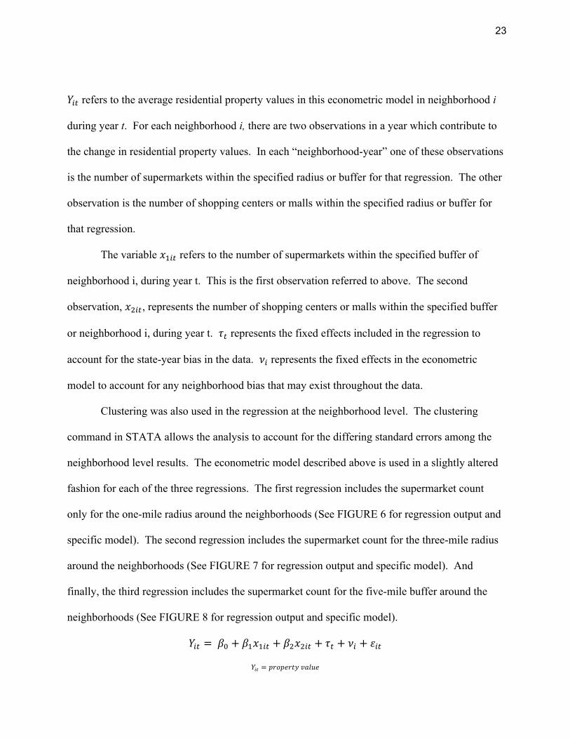
𝑌!" refers to the average residential property values in this econometric model in neighborhood i

during year t. For each neighborhood i, there are two observations in a year which contribute to

the change in residential property values. In each “neighborhood-year” one of these observations

is the number of supermarkets within the specified radius or buffer for that regression. The other

observation is the number of shopping centers or malls within the specified radius or buffer for

that regression.

The variable 𝑥!!" refers to the number of supermarkets within the specified buffer of

neighborhood i, during year t. This is the first observation referred to above. The second

observation, 𝑥!!", represents the number of shopping centers or malls within the specified buffer

or neighborhood i, during year t. 𝜏! represents the fixed effects included in the regression to

account for the state-year bias in the data. 𝜈! represents the fixed effects in the econometric

model to account for any neighborhood bias that may exist throughout the data.

Clustering was also used in the regression at the neighborhood level. The clustering

command in STATA allows the analysis to account for the differing standard errors among the

neighborhood level results. The econometric model described above is used in a slightly altered

fashion for each of the three regressions. The first regression includes the supermarket count

only for the one-mile radius around the neighborhoods (See FIGURE 6 for regression output and

specific model). The second regression includes the supermarket count for the three-mile radius

around the neighborhoods (See FIGURE 7 for regression output and specific model). And

finally, the third regression includes the supermarket count for the five-mile buffer around the

neighborhoods (See FIGURE 8 for regression output and specific model).

𝑌!" = 𝛽! + 𝛽!𝑥!!" + 𝛽!𝑥!!" + 𝜏! + 𝜈! + 𝜀!"

𝑌!" = 𝑝𝑟𝑜𝑝𝑒𝑟𝑡𝑦 𝑣𝑎𝑙𝑢𝑒

VanFossen

24

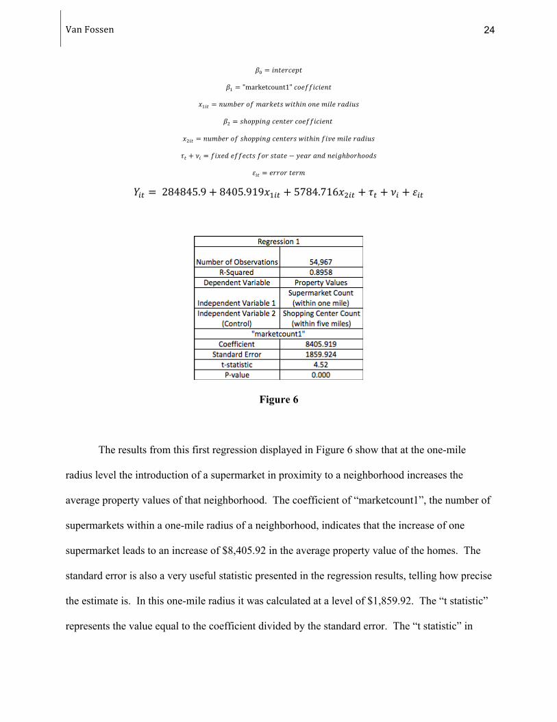
𝛽! = 𝑖𝑛𝑡𝑒𝑟𝑐𝑒𝑝𝑡

𝛽! = "marketcount1" 𝑐𝑜𝑒𝑓𝑓𝑖𝑐𝑖𝑒𝑛𝑡

𝑥!!" = 𝑛𝑢𝑚𝑏𝑒𝑟 𝑜𝑓 𝑚𝑎𝑟𝑘𝑒𝑡𝑠 𝑤𝑖𝑡ℎ𝑖𝑛 𝑜𝑛𝑒 𝑚𝑖𝑙𝑒 𝑟𝑎𝑑𝑖𝑢𝑠

𝛽! = 𝑠ℎ𝑜𝑝𝑝𝑖𝑛𝑔 𝑐𝑒𝑛𝑡𝑒𝑟 𝑐𝑜𝑒𝑓𝑓𝑖𝑐𝑖𝑒𝑛𝑡

𝑥!!" = 𝑛𝑢𝑚𝑏𝑒𝑟 𝑜𝑓 𝑠ℎ𝑜𝑝𝑝𝑖𝑛𝑔 𝑐𝑒𝑛𝑡𝑒𝑟𝑠 𝑤𝑖𝑡ℎ𝑖𝑛 𝑓𝑖𝑣𝑒 𝑚𝑖𝑙𝑒 𝑟𝑎𝑑𝑖𝑢𝑠

𝜏! + 𝜈! = 𝑓𝑖𝑥𝑒𝑑 𝑒𝑓𝑓𝑒𝑐𝑡𝑠 𝑓𝑜𝑟 𝑠𝑡𝑎𝑡𝑒 − 𝑦𝑒𝑎𝑟 𝑎𝑛𝑑 𝑛𝑒𝑖𝑔ℎ𝑏𝑜𝑟ℎ𝑜𝑜𝑑𝑠

𝜀!" = 𝑒𝑟𝑟𝑜𝑟 𝑡𝑒𝑟𝑚

𝑌!" = 284845.9+ 8405.919𝑥!!" + 5784.716𝑥!!" + 𝜏! + 𝜈! + 𝜀!"

Figure 6

The results from this first regression displayed in Figure 6 show that at the one-mile

radius level the introduction of a supermarket in proximity to a neighborhood increases the

average property values of that neighborhood. The coefficient of “marketcount1”, the number of

supermarkets within a one-mile radius of a neighborhood, indicates that the increase of one

supermarket leads to an increase of $8,405.92 in the average property value of the homes. The

standard error is also a very useful statistic presented in the regression results, telling how precise

the estimate is. In this one-mile radius it was calculated at a level of $1,859.92. The “t statistic”

represents the value equal to the coefficient divided by the standard error. The “t statistic” in

25

these results is equal to 4.52. The “p value” is less than 5% or .05 so the results are considered

significant. This p value represents the probability that you would see this distribution in a

regression of random data. Hence, the lower the p value, the more “significant” the results of the

regression. Finally, the “R-squared” value of this regression is equal to 0.8958. The R-squared

value corresponds to the percentage or fraction of variation in the dependent variable that is

accounted for or explained by the independent variable. Thus, the higher the R-value, the more

representative the data is of the econometric model.

𝑌!" = 𝛽! + 𝛽!𝑥!!" + 𝛽!𝑥!!" + 𝜏! + 𝜈! + 𝜀!"

𝑌!" = 𝑝𝑟𝑜𝑝𝑒𝑟𝑡𝑦 𝑣𝑎𝑙𝑢𝑒

𝛽! = 𝑖𝑛𝑡𝑒𝑟𝑐𝑒𝑝𝑡

𝛽! = "marketcount1" 𝑐𝑜𝑒𝑓𝑓𝑖𝑐𝑖𝑒𝑛𝑡

𝑥!!" = 𝑛𝑢𝑚𝑏𝑒𝑟 𝑜𝑓 𝑚𝑎𝑟𝑘𝑒𝑡𝑠 𝑤𝑖𝑡ℎ𝑖𝑛 𝑡ℎ𝑟𝑒𝑒 𝑚𝑖𝑙𝑒 𝑟𝑎𝑑𝑖𝑢𝑠

𝛽! = 𝑠ℎ𝑜𝑝𝑝𝑖𝑛𝑔 𝑐𝑒𝑛𝑡𝑒𝑟 𝑐𝑜𝑒𝑓𝑓𝑖𝑐𝑖𝑒𝑛𝑡

𝑥!!" = 𝑛𝑢𝑚𝑏𝑒𝑟 𝑜𝑓 𝑠ℎ𝑜𝑝𝑝𝑖𝑛𝑔 𝑐𝑒𝑛𝑡𝑒𝑟𝑠 𝑤𝑖𝑡ℎ𝑖𝑛 𝑓𝑖𝑣𝑒 𝑚𝑖𝑙𝑒 𝑟𝑎𝑑𝑖𝑢𝑠

𝜏! + 𝜈! = 𝑓𝑖𝑥𝑒𝑑 𝑒𝑓𝑓𝑒𝑐𝑡𝑠 𝑓𝑜𝑟 𝑠𝑡𝑎𝑡𝑒 − 𝑦𝑒𝑎𝑟 𝑎𝑛𝑑 𝑛𝑒𝑖𝑔ℎ𝑏𝑜𝑟ℎ𝑜𝑜𝑑𝑠

𝜀!" = 𝑒𝑟𝑟𝑜𝑟 𝑡𝑒𝑟𝑚

𝑌!" = 224920.4+ 6056.548𝑥!!" + 3752.007𝑥!!" + 𝜏! + 𝜈! + 𝜀!"

VanFossen

26

Figure 7

The results from the second regression are displayed in Figure 7. In this run of the

regression the main independent variable was the market count with a three-mile radius around

the neighborhoods or “marketcount3” as seen in the table. The coefficient indicates that for

every additional supermarket within the three-mile buffer, residential property values increase by

$6,056.55. The standard error, giving an idea of how precise these results are was calculated at a

level of $1,010.13. The significance of this result is explained in other components of output in

the regression results. The p-value is at a significant level less than .05 of 0.000. The t-statistic

is 6.00 showing that the coefficient is six times as large as the standard error. In addition, the R-

squared value is .8989 meaning the data spread is very close to the constructed econometric

model. Thus, this regression supports that at the three-mile radius supermarkets positively

increase residential property values when introduced in proximity to a neighborhood.

𝑌!" = 𝛽! + 𝛽!𝑥!!" + 𝛽!𝑥!!" + 𝜏! + 𝜈! + 𝜀!"

𝑌!" = 𝑝𝑟𝑜𝑝𝑒𝑟𝑡𝑦 𝑣𝑎𝑙𝑢𝑒

𝛽! = 𝑖𝑛𝑡𝑒𝑟𝑐𝑒𝑝𝑡

𝛽! = "marketcount5" coefficient

𝑥!!" = 𝑛𝑢𝑚𝑏𝑒𝑟 𝑜𝑓 𝑚𝑎𝑟𝑘𝑒𝑡𝑠 𝑤𝑖𝑡ℎ𝑖𝑛 𝑓𝑖𝑣𝑒 𝑚𝑖𝑙𝑒 𝑟𝑎𝑑𝑖𝑢𝑠

𝛽! = 𝑠ℎ𝑜𝑝𝑝𝑖𝑛𝑔 𝑐𝑒𝑛𝑡𝑒𝑟 𝑐𝑜𝑒𝑓𝑓𝑖𝑐𝑖𝑒𝑛𝑡

𝑥!!" = 𝑛𝑢𝑚𝑏𝑒𝑟 𝑜𝑓 𝑠ℎ𝑜𝑝𝑝𝑖𝑛𝑔 𝑐𝑒𝑛𝑡𝑒𝑟𝑠 𝑤𝑖𝑡ℎ𝑖𝑛 𝑓𝑖𝑣𝑒 𝑚𝑖𝑙𝑒 𝑟𝑎𝑑𝑖𝑢𝑠

𝜏! + 𝜈! = 𝑓𝑖𝑥𝑒𝑑 𝑒𝑓𝑓𝑒𝑐𝑡𝑠 𝑓𝑜𝑟 𝑠𝑡𝑎𝑡𝑒 − 𝑦𝑒𝑎𝑟 𝑎𝑛𝑑 𝑛𝑒𝑖𝑔ℎ𝑏𝑜𝑟ℎ𝑜𝑜𝑑𝑠

𝜀!" = 𝑒𝑟𝑟𝑜𝑟 𝑡𝑒𝑟𝑚

𝑌! = 275923.2+ 4144.949𝑥!!" + 2309.332𝑥!!" + 𝜏! + 𝜈! + 𝜀!"

27

Figure 8

The results from the third regression are found above in Figure 8. The count of

supermarkets within the five-mile radius was the main independent variable with the shopping

center count included once again as a control variable. The results showed that an additional

supermarket within a five-mile radius around a neighborhood would on average increase

residential property values by $4,144.95. The standard error, once again giving an idea of how

precise these results are was calculated at a level of $781.64. This result is seen as significant

because the p-value is less than .05. The t-statistic of this regression is 5.30 meaning the

coefficient is 5.3 times as large as the standard error. Furthermore, the “R-squared” value of this

regression is .8997 showing that the econometric model largely explains the distribution of the

data. Again, regression output in this component of the research supported that supermarkets

positively increase residential property values when introduced in proximity to a neighborhood.

In addition to running the three main regressions, one additional model was constructed

in order to determine the effect of each additional grocery store introduced in proximity to a

neighborhood. In order to do this, five dummy variables were created called “shop1”, “shop2”,

VanFossen

28

“shop3”, “shop4” and “shop5”. Shop1 was set to be equal to one if the number of markets in

“marketcount1” was equal to 1 and set to 0 otherwise. Shop2, Shop3, Shop4 were constructed in

the same way except created for their respective numbers in the variable name. Shop5 was

created as a dummy variable equal to 5 for all values in “marketcount1” that were equal to 5 or

greater. One set of fixed effects was used for the neighborhoods in this regression and one was

used for the year. The econometric model for this regression looks as follows in FIGURE 9:

𝑌!" = 𝛽! + 𝛽!𝑥!!" + 𝛽!𝑥!!! + 𝛽!𝑥!!"+ 𝛽!𝑥!!"+ 𝛽!𝑥!!" + 𝜏! + 𝜈! + 𝜀!"

𝑌!" = 𝑝𝑟𝑜𝑝𝑒𝑟𝑡𝑦 𝑣𝑎𝑙𝑢𝑒

𝛽! = 𝑖𝑛𝑡𝑒𝑟𝑐𝑒𝑝𝑡

𝛽! = "shop1" coefficient

𝑥!!" = 1 𝑜𝑟 0 𝑑𝑒𝑝𝑒𝑛𝑑𝑖𝑛𝑔 𝑤ℎ𝑒𝑡ℎ𝑒𝑟 𝑚𝑎𝑟𝑘𝑒𝑡𝑐𝑜𝑢𝑛𝑡1 𝑖𝑠 𝑒𝑞𝑢𝑎𝑙 𝑡𝑜 𝑒𝑥𝑎𝑐𝑡𝑙𝑦 1

𝛽! = "shop2" coefficient

𝑥!!" = 1 𝑜𝑟 0 𝑑𝑒𝑝𝑒𝑛𝑑𝑖𝑛𝑔 𝑤ℎ𝑒𝑡ℎ𝑒𝑟 𝑚𝑎𝑟𝑘𝑒𝑡𝑐𝑜𝑢𝑛𝑡1 𝑖𝑠 𝑒𝑞𝑢𝑎𝑙 𝑡𝑜 𝑒𝑥𝑎𝑐𝑡𝑙𝑦 2

𝛽! = "shop3" coefficient

𝑥!!" = 1 𝑜𝑟 0 𝑑𝑒𝑝𝑒𝑛𝑑𝑖𝑛𝑔 𝑤ℎ𝑒𝑡ℎ𝑒𝑟 𝑚𝑎𝑟𝑘𝑒𝑡𝑐𝑜𝑢𝑛𝑡1 𝑖𝑠 𝑒𝑞𝑢𝑎𝑙 𝑡𝑜 𝑒𝑥𝑎𝑐𝑡𝑙𝑦 3

𝛽! = "shop4" coefficient

𝑥!!" = 1 𝑜𝑟 0 𝑑𝑒𝑝𝑒𝑛𝑑𝑖𝑛𝑔 𝑤ℎ𝑒𝑡ℎ𝑒𝑟 𝑚𝑎𝑟𝑘𝑒𝑡𝑐𝑜𝑢𝑛𝑡1 𝑖𝑠 𝑒𝑞𝑢𝑎𝑙 𝑡𝑜 𝑒𝑥𝑎𝑐𝑡𝑙𝑦 4

𝛽! = "shop5" coefficient

𝑥!!" = 1 𝑜𝑟 0 𝑑𝑒𝑝𝑒𝑛𝑑𝑖𝑛𝑔 𝑤ℎ𝑒𝑡ℎ𝑒𝑟 𝑚𝑎𝑟𝑘𝑒𝑡𝑐𝑜𝑢𝑛𝑡1 𝑖𝑠 𝑒𝑞𝑢𝑎𝑙 𝑡𝑜 𝑜𝑟 𝑔𝑟𝑒𝑎𝑡𝑒𝑟 𝑡ℎ𝑎𝑛 5

𝜏! + 𝜈! = 𝑓𝑖𝑥𝑒𝑑 𝑒𝑓𝑓𝑒𝑐𝑡𝑠 𝑓𝑜𝑟 𝑦𝑒𝑎𝑟 𝑎𝑛𝑑 𝑛𝑒𝑖𝑔ℎ𝑏𝑜𝑟ℎ𝑜𝑜𝑑𝑠

𝜀!" = 𝑒𝑟𝑟𝑜𝑟 𝑡𝑒𝑟𝑚

𝑌!" = 75,415.88+ 5,545.35𝑥!!" + 14,334.5𝑥!!" + 26148.15𝑥!!" + 48558.89𝑥!!"

+ 99033.66𝑥!!" + 𝜏! + 𝜈! + 𝜀!"

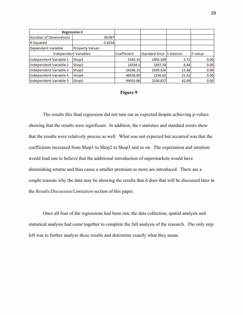
29

Figure 9

The results this final regression did not turn out as expected despite achieving p-values

showing that the results were significant. In addition, the t-statistics and standard errors show

that the results were relatively precise as well. What was not expected but occurred was that the

coefficients increased from Shop1 to Shop2 to Shop3 and so on. The expectation and intuition

would lead one to believe that the additional introduction of supermarkets would have

diminishing returns and thus cause a smaller premium as more are introduced. There are a

couple reasons why the data may be showing the results that it does that will be discussed later in

the Results/Discussion/Limitation section of this paper.

Once all four of the regressions had been run; the data collection, spatial analysis and

statistical analysis had come together to complete the full analysis of the research. The only step

left was to further analyze these results and determine exactly what they mean.

VanFossen

30

6. Results/Discussion/Limitations

The results of this research show that the introduction of a supermarket in proximity to a

neighborhood does increase residential property values on average. It was observed that within

the one mile radius of a neighborhood the introduction of a supermarket will increase residential

property values by around $8,000, within three miles of a neighborhood the introduction of a

supermarket will increase property values by around $6,000 and within five miles of a

neighborhood this price increase is seen at a level of around $4,000. These results show that the

marginal decrease in premium as the radius around the neighborhoods increases meets

expectations that a less conveniently located store would result in less of a premium. Less

conveniently in this context means the stores were located further away on average in the

sample. This difference in premium supports the intuition that a supermarket opening closer to a

neighborhood would have a greater effect on the property values because the shorter distance

makes it more convenient.

It is unclear from the data alone why it is that supermarkets cause these premiums on

homes. This would require a more qualitative analysis to obtain these exact answers and

reasons, but there are several possibilities that could explain why these premiums are occurring.

First and foremost, people enjoy the convenience of having a supermarket nearby. Hence, it

makes sense that the highest premiums occur when supermarkets are introduced closer to the

neighborhood. Proximity of a market provides convenience to a homeowner in ways such as

saving a homeowner time. The proximity of a market will also save a homeowner money that

otherwise would have been spent on gas travelling to a market further away. In addition, the

premium of a supermarket may occur because the market is replacing something that consumers

31

didn’t find as valuable before in the same location. It depends what was in the location of the

supermarket before its entrance, but many times a large grocery store is seen as a very valuable

property when compared to its previous use, which could have been a sporting goods store or

simply just an empty lot. Hence, there are a multitude reasons why a supermarket could be

adding such a premium to a residential property.

We are able to do some estimating on how these premiums occur using some “back of the

envelope” calculations. For example, calculations can be made regarding the money someone

may save in automobile costs (gas, insurance, maintenance, etc…) if a supermarket opens close

to their home, and how this is reflected in the premium on the home. According to the National

Association of Homebuilders’ 2011 study it was determined that the average American lives in a

home for thirteen years (National Association of Home Builders 2011). In addition, according to

an article written by the Hartman Group (a consulting group strictly focused on the food and

beverage industry), looking at U.S. Grocery Shopping Trends in 2016, it was determined that the

average American goes to the grocery store around 1.9 times per week (Hartman Group 2016).

The final piece of information necessary for this quick calculation comes from the American

Automobile Association stating that it costs the average sedan around 59 cents to travel one mile

(AAA 2016). First, let’s convert the years in a home into weeks:

13 𝑦𝑒𝑎𝑟𝑠 × 52 𝑤𝑒𝑒𝑘𝑠1 𝑦𝑒𝑎𝑟 = 676 𝑤𝑒𝑒𝑘𝑠

Next, determine how many trips to the grocery store this would make for an average American

family throughout their stay in a home:

676 𝑤𝑒𝑒𝑘𝑠 ×1.9 𝑔𝑟𝑜𝑐𝑒𝑟𝑦 𝑡𝑟𝑖𝑝𝑠

1 𝑤𝑒𝑒𝑘 ≈ 1,284 𝑔𝑟𝑜𝑐𝑒𝑟𝑦 𝑡𝑟𝑖𝑝𝑠

VanFossen

32

Now, we will add in an assumption that the closest supermarket to a home was previously five

miles away and a new supermarket opens one mile away from the home. This saves a total of

eight miles of driving every time a trip is made to the grocery store (four less miles there and

four less miles back). The next calculation will look into how many miles of driving this will

save over the thirteen years:

1,284 𝑔𝑟𝑜𝑐𝑒𝑟𝑦 𝑡𝑟𝑖𝑝𝑠 ×8 𝑚𝑖𝑙𝑒𝑠 𝑠𝑎𝑣𝑒𝑑1 𝑔𝑟𝑜𝑐𝑒𝑟𝑦 𝑡𝑟𝑖𝑝 = 10,262 𝑚𝑖𝑙𝑒𝑠 𝑠𝑎𝑣𝑒𝑑

The final calculation is to determine how much money this would save using the information

provided by the American Automobile Association:

10,262 𝑚𝑖𝑙𝑒𝑠 𝑠𝑎𝑣𝑒𝑑 ×. 59 𝑑𝑜𝑙𝑙𝑎𝑟𝑠 𝑠𝑎𝑣𝑒𝑑1 𝑚𝑖𝑙𝑒 𝑠𝑎𝑣𝑒𝑑 ≈ 6,055 𝑑𝑜𝑙𝑙𝑎𝑟𝑠 𝑠𝑎𝑣𝑒𝑑

Thus, this calculation shows during the thirteen years on average that the American spends in a

home; if a grocery store opens four miles closer to the home it would probably save around

$6,055 dollars in automobile costs alone. Thus, this quick calculation regarding automobile and

gas costs explains at least part of the premium in housing values that is observed when a

supermarket is introduced in proximity to a neighborhood.

While the results do show that there is a correlation between supermarket entry and

residential property values there are several limitations to this research that must be addressed.

The first limitation of the research corresponds to the quality, quantity and location of the

neighborhood data. Figure 1 displays a visual representation of the spread of neighborhood data

across the country. Although the data does cover many different parts of the country, there are

many large stretches of the nation that have no property value data. It appears as though the data

favors more urban areas and their surrounding suburbs. Zillow is a for-profit organization and it

33

is in their interest to target wealthier areas that are more densely populated. For this reason,

certain land demographics are largely excluded from the data in favor of more populated areas

across the country.

Another limitation of the study is the quality of the neighborhood data. It is very difficult

to create a database of housing prices across an area because it is hard to simply declare the

actual price of a house. The only way to determine this is when a house is sold, and every home

isn’t sold every year. If that were the case, this dilemma would be solved. Zillow’s Zestimates

are an attempt at creating an accurate database by avoiding the fallacy of using the values of only

the sale prices from that year. The “Zestimate” uses a computer based algorithm to determine

the average home prices, but according to a 2014 study by Charles Corcoran titled, “Accuracy of

Zillow’s Home Value Estimates,” the estimates are not so accurate, ranging from a “17.15% to

30.48% premium at times” (Corcoran 2016). Thus, the quality of the property value data is also

brought into question as a possible limitation in the research.

In the research, another limiting factor could have been the absence of other potential

control variables. The main control in this research was the commercialization that is usually

correlated with the introduction of a supermarket. In order to control for this commercialization,

the introduction of shopping centers and malls were also used as an independent variable in the

regressions. Although there was this control used in the research there are other control variables

that potentially could have been used that are correlated with supermarket entry and property

values. Examples of such variables could be the openings of schools, parks, museums,

apartment/condominium complexes, etc. Hence, there potentially could be further controls taken

into account in this research.

VanFossen

34

Regarding the fourth and final regression, the discrepancy in the results versus the

expectation could be caused because the areas with more supermarkets tend to be wealthier

areas. The average residential property value of neighborhoods with exactly one supermarket is

$183,695 and the average for neighborhoods with 5 or greater supermarkets is $362,160, almost

twice as expensive. Therefore, the Shop5 variable being equal to one was largely correlated with

much wealthier areas resulting in a larger premium. This larger premium most likely occurs

because people with more money are willing to pay more for a convenience such as a nearby

grocery store. Another reason is because if the premium works partly in terms of a percentage of

the housing prices, then an area with a higher home value on average will result in higher

premiums. Thus, the correlation with areas that are already affluent may be one reason why the

data presented the coefficients that it did. The other main reason for these results may be a

problem of omitted variables in the regression. As an area builds a fourth or fifth supermarket

there may be something else occurring in the area that is not controlled for in the data. Hence,

further research could be able to find and determine exactly what may be occurring in

conjunction with the introduction of these later markets that would explain these unexpected and

rather large premiums.

7. Concluding Remarks

Despite the limitations of the research, the results do show that the introduction of a

supermarket in proximity to a neighborhood increases its average residential property values.

Although this main question has been answered, there are still many more questions to be

answered in further research regarding the topic. Further research could more effectively

35

determine how the “value-add” of a supermarket changes when the number of pre-existing

markets within the buffer changes. The expected result would be that a supermarket entering an

area with zero supermarkets would present a much greater premium on residential property

values than one that entered an area that already had three supermarkets. Further research could

also determine the effect of a supermarket in different regions of the country. It could be that

some regions of the nation value the convenience of having a supermarket nearby more than

others. There are countless further questions that could be explored in this dynamic between the

supermarket and residential properties. Thus, this research answers the question of how the

supermarket and the neighborhood interact on a monetary level in one sense, but there are still

many questions to answer and different ways to approach investigating this dynamic.

VanFossen

36

Works Cited

AAA. Your Driving Costs: How Much Are You Really Paying to Drive?, American Automobile

Assocation, 2016. Print.

Bruce, Andrew. "Zillow Home Value Index: Methodology." Zillow Research. Zillow Group, 03

Jan. 2014. Web.

Cardwell, Diane. "A Plan to Add Supermarkets to Poor Areas, With Healthy Results." The New

York Times. 23 Sept. 2003. Web.

Corcoran, Charles, and Fei Liu. "Accuracy of Zillow’s Home Value Estimates." Real Estate

Issues 39.1 (2014): 45-49. Web.

Hartman Group. "U.S. Grocery Shopping Trends, 2016." The Hartman Group (2016): 1-38.

Web.

Lea, Scott. Business Data Assets. Papillion, NE: InfoGroup, 2017. Print.

Li, Mingche M., and H. James Brown. "Micro-Neighborhood Externalities and Hedonic Housing

Prices." Land Economics 56.2 (1980): 124-41. The University of Wisconsin Press

Journals Division. Web.

Lloyds Bank. Living Near a Supermarket Can Bag You a 22,000 Bonus On Your Home. Lloyds

Banking Group. Lloyds Bank, 25 July 2016. Web.

37

Martinez, L. Miguel, and Jose Manuel Viegas. "Effects of Transportation Accessibility on

Residential Property Values." Journal of the Transportation Research Board 2115.16

(2009): 127-37. TRR Journal Online. Web.

National Association of Home Builders. Economics and Housing Policy. Latest Calculations

Show Average Buyer Expected to Stay in a Home 13 Years. HousingEconomics.com. 3

Jan. 2013. Web.

"North American Industry Classification System." United States Census Bureau. U.S. Census

Bureau, 2 Mar. 2017. Web.

"ReferenceUSA - Data Quality." ReferenceUSA. InfoGroup Incorporated, 2017. Web.

Smith, Rosa Inocencio. "When a Grocery Store Means Gentrification." The Atlantic. 16 Aug.

2016. Web.

Thibodeau, Thomas G. "Estimating the Effects of High Rise Office Buildings on Residential

Property Values." Land Economics 66.4 (1990): 402-08. University of Wisconsin Press

Journals Division. Web.

VanFossen

38

Datasets

ReferenceUSA, InfoGroup (2016). Supermarkets in United States 1997-2015 Historical Business

(Academic Version). Wharton Research Data Service. https://wrds-

web.wharton.upenn.edu/

ReferenceUSA, InfoGroup (2016). Shopping Centers and Malls in United States 1997-2015

Historical Business (Academic Version). Wharton Research Data Service. https://wrds-

web.wharton.upenn.edu/

Zillow Group (2016). Zillow Home Value Index (ZHVI), 1997-2015, All Homes Version,

Neighborhood Level. Seattle, Washington. https://www.zillow.com/research/data/

39