the weight of residential investment in the french economy...
TRANSCRIPT

1
The weight of residential investment in the French economy
Asma Ben SAAD (Corresponding Author)
Laboratoire d’Economie d’Orléans (LEO), Université d’Orléans, Rue de Blois BP : 26739.
45067 – Orléans Cedex 2
E-mail:[email protected]
Muhammad KHAN
Laboratoire d’Economie d’Orléans (LEO), Université d’Orléans, Rue de Blois BP : 26739.
45067 – Orléans Cedex 2
E-mail: [email protected]
Abstract: The recent subprime crisis attracts the attention of the policymakers on the role of real estate in
economic stability. This paper evaluates the weight of residential investment in the French economy
using a quarterly data set from 1950Q2 to 2013Q1. Our main results, deduced by the Leamer’s
methodology (2007) and based on the rolling regression models and the structural vector autoregressive
models, show that the contribution of real estate sector in the French GDP reduction is both negligible
and decreasing over-time. Shocks to residential investment, thereby, do not appear to pose any serious
problem to the macroeconomic stability in France.
Keywords: Real estate, financial stability, GDP Growth.
Jel Classifications: E32, L85, E44

2
1. Introduction:
Since the inception of the recent subprime crisis of 2007, economists started inquiring
about the role of real estate in the economic performance of countries with developed financial
systems. It is usually argued that in order to assure financial stability, the policymakers need to
use macroprudential measurements in the property market.1 Taking into account the
heterogeneity of the property markets which includes their institutional framework, economic
characteristics, intervention of the public authorities and financing conditions, the weight of the
residential investment in the economic evolution differs from one country to another.
Accordingly, the macroprudential policies aimed at controlling the fluctuation in the real estate
market also need to be granular across countries and regions (Hartmann, 2015).
The economic literature usually focuses on the importance of real estate sector in the
domestic GDP growth as well as in international financial stability. Due to the significant share
of real estate in the economic growth of certain countries, changes in its price (or volume) exert
considerable long-term consequences for these economies. Coulson and Kim (2000) note that the
residential investment influences the evolution of the U.S GDP. Bernanke (2007) also confirms a
strong link between residential investment and economic activity for the U.S economy.
Cardarelli et al., (2008) show that the development of real estate financing system intensifies the
impact of monetary policy on the residential investment and housing prices.
Applying the impulse response function, on the U.S data set from 1959 to 2007, Miles
(2009) shows that the impact of the residential investment is particularly high after 1980s. Liu
and others (2002) use Chinese data set from 1981 to 2000 and show that the residential
investment strongly influences the economic fluctuation, although its weight does not exceed
8.6% of the GDP. Álvarez et al., (2010) posit that the residential investment can be used as an
indicator of the evolution of GDP. Their study finds asymmetry in the effects of residential
1 In general, the evolution of real estate sector is measured by the indicators like residential investment, the real
estate prices and the building stock.
3
investment on GDP growth; expansionary periods play a more important role in the evolution of
the GDP than the recessionary episodes of the same magnitude.
With the advent of the financial crisis of 2007, a bulk of empirical literature has been
devoted to the topic; albeit, focusing mainly on the three developed economies; Spain, the United
Kingdom and the United States (Leamer 2007; Bernanke 2007; Timbeau 2014). Generally, this
literature shows a positive relationship between residential investment and economic growth.
Coming to the French housing sector, there exists a dearth of work on the subject. This can be
explained by an apparently weak impact of the current (subprime) crisis on the evolution of
French residential investment; compared to the above-mentioned economies. Cardarelli and
others (2008) note that during the last decade the share of residential investment in the French
GDP growth remained only around 5%. Ferrara and Vigna (2009) argue that the French
economy benefitted from two structural characteristics to avoid a collapse of its property market;
the application of fixed loan rate and the moderate debt level of the households.2 Boulhol (2011)
focuses on the importance of real estate in the French economy, in particular the weight of real
estate debt in the household budget. The author finds contradictory evidence from the above by
noting that the contribution of mortgage expenditures in the households’ spending has increased
significantly since 1980. In 2000, nearly 20% income of the middle class families has been
allocated for the repayment of real estate purchase.
The conflicting views about the relevance of the real estate sector for the French GDP
growth necessitate further inquiry into the subject. Besides, the recent trends in the real estate
markets have also been considered unusual and the concerning authorities of the financial
stability started constantly supervising the evolution of the housing sector indicators; especially
the real estate prices. The High Board of Financial Stability (Haut Conseil de Stabilité
Financière) which observes the conditions of the housing credit, mentions in the report of the
“council of financial regulation and systemic risk” that the eruption of real estate crisis in the
United States, the United Kingdom and Spain has alerted the French authorities forcing them to
reevaluate the performance of the real estate sector (Corefris, 2011).3 This specific focus on the
2 It is important to note that since the years 2000, the credit granting conditions are increasingly flexible in France
with more duration of credit length and lower interest rates. To illustrate, the duration of the credit increased from 14
years in 1999 to 20 years in 2012 (Avouyi‑Dovi and al., 2014). Despite these easy loan facilities, the level of
households’ debt remained moderate compared with the other western countries. 3Corefris is replaced by the High Board of financial stability since July 2013.
4
real estate sector has also been motivated by the contemporaneous research (e.g., Leamer, 2007)
which finds its significant contribution in triggering recession among the other sectors including
the spending by consumers, the business, the government and the external sectors of the U.S
economy. More importantly Leamer reports this unique behavior of housing sector by arguing,
“Housing is the biggest problem in the year before recession, but is the first to start to improve
in the second quarter of the recession” (Leamer 2007, p.16).
Against this backdrop, our main task is to explore whether the French real-estate market
indeed requires the use of macroprudential measurements for managing the real estate cycles.
Certainly, the use of macroprudential tools is justified only if the residential investment
significantly contributes to the GDP growth reduction in France. That said we also aim to see
whether the contribution of real estate sector in the fluctuations of the French GDP growth has
changed over-time. A time-varying rolling regression model helps us to answer this question.
Lastly, we test the persistence of shocks by using a structural vector autoregressive model. For
our empirical investigation, we measure the cumulative abnormal contribution of the residential
investment to the GDP growth before and after a peak by applying the Leamer’s (2007, 2009)
methodology. This allows us to separately analyze the negative contribution of residential
investment in reducing the GDP growth, for our selected time period from 1950Q2 to 2013Q1.
Our empirical results illustrate a weak contribution of the residential investment to the GDP
reduction in France before and after the recessionary periods. Furthermore, this contribution
significantly reduces during the recent decades.
The rest of the paper is structured as follows. Section 2 outlines the structural vector
autoregressive model for the French economy. Section 3 presents the selected data set used in
this study. Section 4 reports the summary of our main findings. Section 5 offers conclusion.
2. Structural Vector Autoregressive model (SVAR model)
In order to estimate the effects of residential investment shocks on the French GDP growth
and its components, we estimate a structural vector autoregressive (SVAR) model. The SVAR
methodology facilitates us in analyzing both the magnitude as well as the persistence of changes
in the GDP to shocks in real estate market and other variables. A main advantage of this
approach is that by using this methodology we can model the non-recursive structure of the
economy and thus interpret the contemporaneous correlations of disturbances. Effectively, a

5
decomposition of variance-covariance matrix using a SVAR model yields a recursive scheme
among variables that has clear economic implication and that can be tested as any other
relationship (see Mamoudou et al., 2009).
An important step in the SVAR model is the selection of an appropriate number of
covariates. As we are interested to analyze the effects of shocks to residential investment on the
French GDP, several other growth covariates including inflation, short term interest rate,
European GDP –for external shocks – and the real exchange rate, etc. could also be included.
However, all these relevant covariates were not incorporated mainly for two reasons; first, the
information on these variables was not available for the whole sample period and second, by
adding more variables, the size of our SVAR model could become larger and, thereby, difficult
to manage. Consequently, our SVAR model only explains how shocks to different components
of the GDP including residential investment, imports, exports and household consumption
impact the GDP growth in France. The selected open economy can be represented by the
following structural form equation:
1( )t t tBX C L X u (1)
where
'
1( ) , ( ' ) 0, 0,t t t tE u u D E u u s
B is a nonsingular matrix that is normalized to have 1s on the diagonal, Xt is an ‘n x 1’vector of
the above-mentioned included variables, C(L) is polynomial in the lag operator L, and ut is an
1n vector of structural disturbances. D is a diagonal matrix whose off-diagonal elements are
zero and whose diagonal elements are variances of structural disturbances.
As matrix Xt comprises endogenous variables, its estimation using OLS yields biased and
inconsistent results. The solution lies in estimating a reduced form model in order to get
maximum likelihood estimates of B and D. Mathematically:4
1( )t t tX A L X (2)
4See Lawson and Rees (2008) for a detail description of the model.
6
where '( )t tE .
The structural disturbances and the reduced-form residuals are related by t tu B
implying that:
' '( )t tD E B B (3)
From equation (3), B and D can be recovered by imposing certain restrictions on some of
the contemporaneous relationships between the included variables. Conventionally, the
economic literature follows the method of Cholesky decomposition where reduced-form
disturbances are orthogonalised by implying a recursive temporal ordering of the variables.
However, Cooley and LeRoy (1995), criticize this method because of its deficiency in finding a
theoretically valid causal structure. The alternative is to use the theoretical reasoning and
assuming that changes in some variables affect the others only after some lags. We adopt this
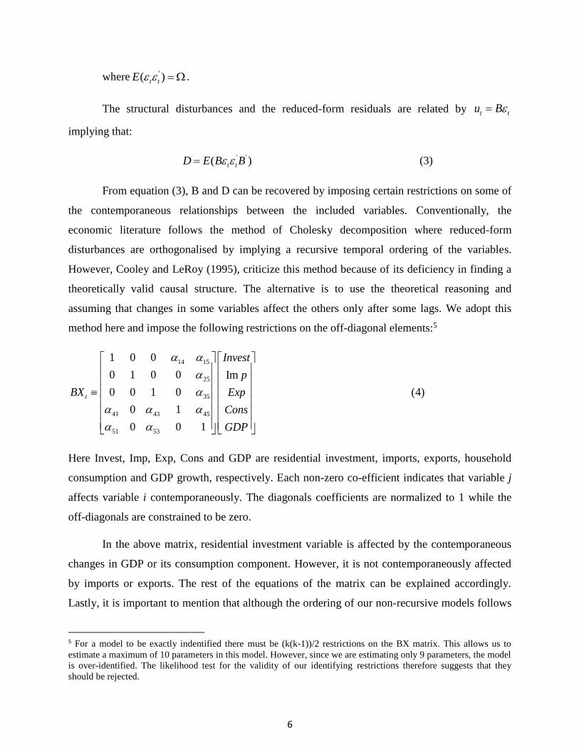
method here and impose the following restrictions on the off-diagonal elements:5
14 15
25
35
41 43 45
51 53
1 0 0
0 1 0 0 Im
0 0 1 0 (4)
0 1
0 0 1
t
Invest
p
BX Exp
Cons
GDP
Here Invest, Imp, Exp, Cons and GDP are residential investment, imports, exports, household
consumption and GDP growth, respectively. Each non-zero co-efficient indicates that variable j
affects variable i contemporaneously. The diagonals coefficients are normalized to 1 while the
off-diagonals are constrained to be zero.
In the above matrix, residential investment variable is affected by the contemporaneous
changes in GDP or its consumption component. However, it is not contemporaneously affected
by imports or exports. The rest of the equations of the matrix can be explained accordingly.
Lastly, it is important to mention that although the ordering of our non-recursive models follows
5 For a model to be exactly indentified there must be (k(k-1))/2 restrictions on the BX matrix. This allows us to
estimate a maximum of 10 parameters in this model. However, since we are estimating only 9 parameters, the model
is over-identified. The likelihood test for the validity of our identifying restrictions therefore suggests that they
should be rejected.

7
the economic theory, the estimated results of the SVAR model are robust with respect changes in
this ordering.
3. Data
The National Institute of Statistics and Economic Studies (INSEE, hereafter) provides
data set on the GDP and its components starting from the second quarter of 1950 to 2012.6 The
data are expressed in volumes at the chained prices of the previous year – seasonally adjusted
and corrected for working days–using 2005 as base year. To evaluate the contribution of the
residential investment around the peak value of GDP, we apply Leamer (2007, 2009) method
which consists of three steps: i) extract the normal component, ii) determine the abnormal
component, and finally, iii) standardize the series.
Following majority of the above-mentioned studies, we use the Hodrick-Prescott (HP)
filter with the value of smoothing parameter as λ= 1600 (for quarterly data) to extract the trend
from our series.7 To get the “abnormal” component of GDP, we subtract the normal series (the
trend component) from the original data. Similarly, we estimate the cumulated abnormal
contribution of each component of the GDP, expressed in percentage points. To determine the
turning points of the GDP series, we use the algorithm Harding and Pagan (2002): “the Bry-
Boschan algorithm for quarterly data” (BBQ).
Thereafter, we analyze the evolutions of each component compared to the peak dates.
For this step, we process the data by interval: for each peak, we select the data for N periods
before the peak and K periods following the peak. The choice of the duration of the two periods
is arbitrary. In the present case we consider the contribution of the components one year before
6The components of GDP comprise : import, export, Household final consumption expenditure , final consumption
expenditure of general government of which individual consumption expenditure, final consumption expenditure of
general government of which collective consumption expenditure, final consumption expenditure of non-profit
institutions serving households, gross fixed capital formation (GFCF) of general government, GFCF of non-financial
corporation and unincorporated enterprise, GFCF of financial corporation and unincorporated enterprise, GFCF of
households excluding unincorporated enterprise, GFCF of non-profit institutions serving households and changes in
inventories. 7For robustness purposes we also apply a second filter, known as Baxter and King filter, with an interval of [6.32]
quarters to check whether the choice of the filters influences our main results.

8
the peak and four years after the peak. Then, within each interval, we subtract the value of the
peak, resulting in a zero value for all the peak points. Finally, to calculate the cumulative
abnormal contribution of each component to the reduction of GDP, we make the sum of the
negative contributions for each component. Any positive contribution is replaced by zero value.
Table 1 : Contributions to GDP growth
Time
GDP (%) Import(-) Consumption
Residential
Investment Investment
Inventory
change Export
1951T1 0.104 0.400 1.330 0.263 0.993 -1.804 -0.016
1961T1 1.288 0.020 1.620 0.197 1.111 -1.613 0.188
1971T1 1.614 -0.203 0.837 0.587 0.707 -0.483 0.351
1981T1 0.302 -0.206 0.212 -0.081 -0.190 -0.362 0.435
1991T1 -0.029 0.287 0.114 -0.141 -0.176 0.249 0.071
2001T1 0.576 -0.311 0.581 0.036 0.147 -0.614 0.150
2011T1 1.104 1.243 0.187 -0.012 0.275 1.385 0.500
Source: INSEE
Table 1 shows the contribution of all components of GDP for some selected data points
in every ten years (average duration of a GDP cycle). As can be noticed, the GDP growth in first
quarter of 1971 is 1.6% of which the contribution of residential investment is 0.5 (Percentage
Point) and that of export is of 0.3 (Percentage Point). The sum of the contributions of
components is equal to the growth rate of GDP for the same period. In 2011, the growth rate of
the GDP is about 1.104% resulting from the sum of contribution of consumption (0.187),
investment (0.275), inventory change (1.385) and export (0.5) minus the contribution of the
imports (1.243).
The small contribution of residential investment to GDP growth, however, does not
reflect the weight of residential investment during recessions or expansions periods. Learner
(2007) also finds a small contribution of the US residential investment to the GDP growth.
Nevertheless, due to the weight of residential investment in the U.S recessions or expansions, the
author argues that ‘the American business cycle is the housing cycle’.
4. Results and discussion:
By employing the BBQ algorithm on detrended series of our HP filter, we could identify
the following peaks: 1957Q3, 1963Q3, 1974Q1, 1980Q1, 1990Q1, 2001Q1 and 2008Q1.8 With
8By using the Baxter and King filter, the peak dates sometimes shifted by one or two quarters and we get the
following peak points: 1957Q4, 1964Q1, 1974Q2, 1979Q4, 1989Q4, 2000Q4 and 2008Q.

9
this information we measure the cumulative abnormal contribution of each component to the
sluggishness of the GDP for our selected time period and find that on average the residential
investment contributes to 10% downwards movement of the GDP growth one year before the
peak.9 On average, the GDP growth observed a reduction of merely 1.67%. The main
components responsible for this GDP reduction include exports, the inventory changes and the
investment of the non-financial companies with their shares of 30%, 19% and 16%, respectively.
Figure (1) presents the contribution of the four main components to the French GDP growth
before and after the peaks since 1950.10 The abscissa axis of this graph represents five years
period (twenty quarters) around a peak. The point 0 indicates the date of the peak, the period
before the peak ranges between [- 4, - 1] and the four years following the peaks are between [1,
16].The ordinate axis presents the average of cumulative abnormal contributions from one
component of the GDP growth. Through the figure (1), we can also determine the component
that, on average, contributes most to the fall in GDP in the seven peaks, defined earlier.
Figure1: Cumulative Abnormal Contribution to GDP Growth
Source: Authors’ calculation
According to our results, for both pre- and post-peak periods, the export component
brings the largest contribution in the reduction of GDP. For the year before the peak, its
contribution is 0.6% while the one from the residential investment is merely 0.2%. Four quarters
9Cardarelli and al. (2008) report similar results for their sample of 1970 to 2007. The authors note that during the
French recession of 2OO2-T3 to 2OO3-T2, the residential investment only contributed 4% of cumulated downwards
movement of the GDP whereas this contribution was 25% and 13% for the U.S and the U.K, respectively. 10These include exports, final consumption expenditure of households, GFCF of non-financial corporation and
unincorporated enterprises, GFCF of households excluding unincorporated enterprises, changes in inventories.

10
after the peak, the adverse contribution of export reaches its extreme value (nearly 1.5%),
whereas the residential investment does not contribute more than 0.4%. By calculating the
average contribution of the residential investment for the seven peaks, we note that the impact of
the later on the evolution of the GDP is limited.11 Briefly, residential investment occupies the
fourth place in contributing to average GDP sluggishness after export, stocks and the household
consumption, respectively; irrespective of the choice of the filter (see Appendix A: Table A2).
In order to see whether the contribution of residential investment in the GDP reduction
has remained persistent over time or not, we separately analyze this contribution for all of the
detected peak points. The results are shown in Table 2. As can be seen, for the first four peaks
(1957, 1963, 1974, 1980), the cumulated GDP reduction, one year prior to peak, remains 2.03%.
The residential investment, however, contributes only 15% to this fall. During the last three
detected peaks (1990Q1, 2001Q1 and 2008Q1) the cumulated GDP reduces by 1.2%, and the
contribution of residential investment appears to be a negligible 3%. This indicates a structural
break in the relationship between residential investment and the GDP reduction before and after
the 1990s. In other words, the growth inhibiting role of residential investment diminishes after
1990s. On the other hand, the cumulative negative contribution of export as well as non-financial
companies, one year before a peak, accentuates at the end of the 1980s. The impact of the last
two components on the GDP growth seems much more important than the residential investment
during the last three peaks.
Contrary to the cumulative abnormal contributions one year before the peak, the average
weight four years after the peak shows certain regularity. This can be noticed from Table 3. The
cumulative abnormal contribution shows an increasing share of export in the GDP reduction.
About the residential investment, its average contribution does not change and remains stable
around 10%: except for the two time periods 1957-Q3 and 2001-Q1 where it reduces down to
3% and 4%, respectively.
11 For robustness purposes, we determine the normal contribution of the components by applying a filter of Baxter
and King. As the table in the annex indicates, the choice of the filter does not really alter our results.

11
Source: Author's calculations from the methodology Learner (2007), HP filter
Table 3: Cumulative Abnormal Contribution in reducing the GDP, four years after the peak
turning
point
indicator (pic)
Export Changes
in
inventories
Gross Fixed Capital Formation final consumption expenditure
Import GDP
Growth
(%) Residential investment
non-profit
institutions
serving households
Public Administration
financial corporation
and
unincorporated enterprise
non-financial corporation
and
unincorporated enterprise
Household
Non-profit
Institutions Serving
Households
General
Government
of which Individual
Consumption
Expenditure
General
Government
of which Collective
Consumption
Expenditure
57T3 12% 24% 16% 0% 0% 0% 4% 21% 0% 0% 0% -23% -1,04
63T3 16% 17% 18% 0% 7% 1% 10% 28% 0% 3% 0% 0% -3,14
74T1 33% 41% 14% 0% 0% 1% 6% 5% 0% 1% 0% 0% -2,25
80T1 17% 39% 9% 0% 4% 0% 30% 1% 1% 0% 0% 0% -1,68
90T1 29% 6% 4% 0% 0% 2% 19% 21% 1% 8% 4% -6% -1,12
01T1 55% 4% 0% 0% 1% 0% 15% 4% 0% 1% 0% -21% -1,11
08T1 54% 0% 6% 0% 0% 4% 35% 2% 0% 0% 0% 0% -1,43
Average 30% 19% 10% 0% 1% 1% 16% 12% 0% 2% 1% -8% -1,68
Source: Author's calculations from the methodology Learner (2007), HP filter
Table 3: Cumulative Abnormal Contribution in reducing the GDP, four years after the peak
turning point
indicator
(pic)
Export
Changes
in inventories
Gross Fixed Capital Formation final consumption expenditure
Import
GDP
Growth (%)
Residential investment
non-profit institutions
serving households
Public Administration
financial corporation
and
unincorporated enterprise
non-financial corporation
and
unincorporated enterprise
Household
Non-profit
Institutions Serving
Households
General Government
of which Individual
Consumption
Expenditure
General Government
of which Collective
Consumption
Expenditure
57T3 6% 12% 3% 0% 3% 0% 7% 54% 1% 8% 5% 0% -4,74
63T3 10% 16% 9% 0% 2% 2% 14% 40% 0% 1% 2% -5% -2,59
74T1 24% 28% 13% 0% 0% 2% 14% 16% 1% 1% 0% 0% -5,81
80T1 24% 39% 9% 0% 1% 2% 9% 14% 0% 2% 0% 0% -3,25
90T1 29% 16% 14% 0% 1% 2% 14% 24% 0% 1% 0% 0% -3,08
01T1 49% 9% 4% 0% 5% 3% 16% 13% 0% 0% 1% 0% -4,18
08T1 46% 9% 11% 0% 1% 2% 22% 8% 0% 0% 0% 0% -5,14
Average 28% 17% 10% 0% 2% 2% 13% 24% 0% 2% 1% -1% -4,11

12
In what follows, we will be interested only in the residential investment and its
contribution in the GDP diminution before and after a peak period. Figure (2) illustrates the
cumulative abnormal contribution of the residential investment in the GDP growth around peaks.
As can be noticed, since the beginning of the sample period, the average contribution of the
residential investment to GDP reduction remains weak. Indeed, the maximum contribution of
residential investment in the year before 1990 does not exceed 0.2% whereas in 1968 its
contribution downwards of the GDP remains above 0.6%. Moreover, most of our peak points can
be connected with some international events and national decisions. These include the first oil
price shock (1973), the credit restriction of 1973 to 1985, the financial deregulation (1984) and
the Gulf War (1990). All of these events inevitably influenced the consumption and investment
behavior and certainly affected the contribution of components to economic growth. But the
most important change has been ‘the boom’ of innovation in the means of mortgages financing
which has impacted both the real sector and the overall economic growth, particularly starting
from the mid-1980s. It is usually held that within the Euro zone, the relation between the real
sector and the economic growth strengthened with the financial deregulation.12
Figure 2: Cumulative Abnormal Contribution of residential investment to reducing GDP before and since a peak
Source: Authors’ Calculations
12Dynan et al. (2005) support this view for the U.S by showing that innovation in credit financing system had
weakened the link between the U.S real estate and economic activity during the 1980s. They explain how the
diversity of the funding sources had allowed an effective distribution of the risk between the economic agents.
13
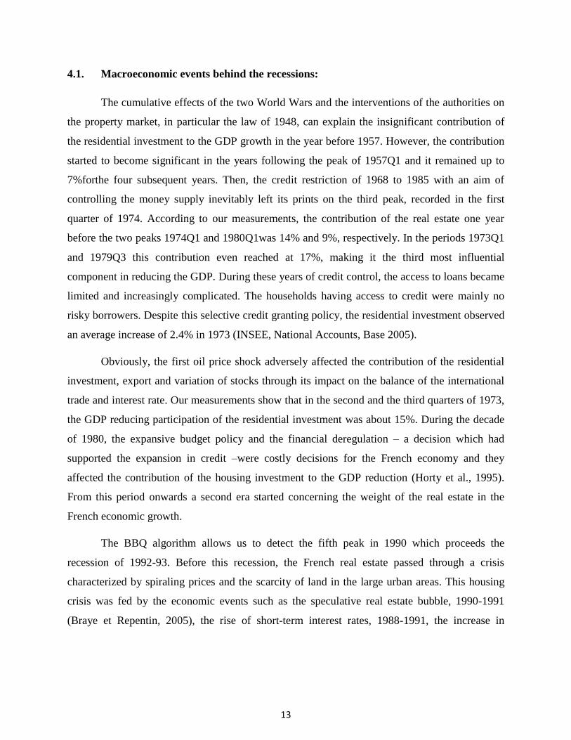
4.1. Macroeconomic events behind the recessions:
The cumulative effects of the two World Wars and the interventions of the authorities on
the property market, in particular the law of 1948, can explain the insignificant contribution of
the residential investment to the GDP growth in the year before 1957. However, the contribution
started to become significant in the years following the peak of 1957Q1 and it remained up to
7%forthe four subsequent years. Then, the credit restriction of 1968 to 1985 with an aim of
controlling the money supply inevitably left its prints on the third peak, recorded in the first
quarter of 1974. According to our measurements, the contribution of the real estate one year
before the two peaks 1974Q1 and 1980Q1was 14% and 9%, respectively. In the periods 1973Q1
and 1979Q3 this contribution even reached at 17%, making it the third most influential
component in reducing the GDP. During these years of credit control, the access to loans became
limited and increasingly complicated. The households having access to credit were mainly no
risky borrowers. Despite this selective credit granting policy, the residential investment observed
an average increase of 2.4% in 1973 (INSEE, National Accounts, Base 2005).
Obviously, the first oil price shock adversely affected the contribution of the residential
investment, export and variation of stocks through its impact on the balance of the international
trade and interest rate. Our measurements show that in the second and the third quarters of 1973,
the GDP reducing participation of the residential investment was about 15%. During the decade
of 1980, the expansive budget policy and the financial deregulation – a decision which had
supported the expansion in credit –were costly decisions for the French economy and they
affected the contribution of the housing investment to the GDP reduction (Horty et al., 1995).
From this period onwards a second era started concerning the weight of the real estate in the
French economic growth.
The BBQ algorithm allows us to detect the fifth peak in 1990 which proceeds the
recession of 1992-93. Before this recession, the French real estate passed through a crisis
characterized by spiraling prices and the scarcity of land in the large urban areas. This housing
crisis was fed by the economic events such as the speculative real estate bubble, 1990-1991
(Braye et Repentin, 2005), the rise of short-term interest rates, 1988-1991, the increase in

14
unemployment rate, the excess of savings, the elevated level of companies’ debt.13 This situation
was not favorable for investment, and it resulted in a reduction of growth rate from 2.8% to 0.2%
from 1989Q2 to 1990Q1 (INSEE). Precisely, our estimations show that the contribution of the
residential investment to recessions strongly reduced since 1989Q2. This can appear from two
factors; first, the lower overall volume of the residential investment and second, a more prudent
and risk averse behavior of the French financial institutions.
The mere 4% prior to peak contribution of residential investment in the GDP growth
enables us to argue that the former does not pose any threat to the economic stability. Regarding
the four quarters afterwards effects, we notice that between 1991Q2 and 1992Q2 the contribution
of the residential investment has raised and reached at 33% in 1992Q1. But this unfavorable
contribution was rectified at the end of the four quarters to reach at 11%, making the four year
average contribution at 15%. This contribution, being highest since 1950, relates with the French
recession of 1993. Therefore, we can conjecture that even in the adverse economic
circumstances, the contribution of the residential investment in the GDP reduction was not so
alarming. Finally, in the crisis of 2001, the role of residential investment appears insignificant
both before and after the crisis. These results can be explained by the origin of the deceleration
which is none other than the Internet bubble (Leamer, 2009).
The results also show that the intensity of the adverse effects of residential investment on
the GDP growth weakened over-time. In other words, the contribution of the real estate in
reducing the GDP growth seems to appear in two phases: the first phase starts in 1950 till the end
of 1980 and the second phase starts from 1990. The behavior of the French residential
investment in these two periods is systematically different from one another: the first period is
characterized by strong fluctuations and a high growth rate (nearly 12%) and then starting from
1980s, the evolution of the residential investment is not very volatile though the cycles remain
longer than the first phase. For robustness of our results, in the first step, we adopt a rolling
regression analysis, and in the second step, a SVAR model.
13 Households save more than they consume in order to mitigate the impact of a potential unemployment. This
saving behavior generates excessive saving (Horty, 1995).

15
4.2. The real estate and the GDP growth changes: rolling regression analysis
Our analysis heretofore explain two main aspects of the relationship between the French
residential investment and GDP growth; first, the contribution of weakness of the residential
investment to the economic sluggishness has not been so important in most of the recessionary
episodes and second, this contribution has not remained stable and rather reduced over time.
However, this descriptive analysis of different recessionary periods does not provide a concrete
picture of the relationship over the whole sample period. To get a more solid depiction of this
relationship and to capture the time variation in it, we use a rolling regression approach. To this
end, we test the connection between the cyclical changes of the residential investment and the
GDP growth. A main advantage of our rolling regression technique is that here the coefficients
of each sub-sample are completely independent and therefore allow greater flexibility in
detecting the structural changes in this relationship over time. Our rolling regressions are based
on the fixed window size of 100 quarters, the first regression is run by using the first 100
observations and then the window moves downwards by excluding the first observation of the
sample and including the next quarter in the sequence. A constant window size enables us to
compare the coefficients across samples. As we are interested to see the structural changes with
respect to time, we retain the same temporal ordering of our sample.

16
-20
24
Be
ta I
nves
tme
nt
0 50 100 150time
_b[Invest] lower/upper
-10
12
3
Be
ta I
nve
stm
en
t
0 50 100 150time
_b[Invest] lower/upper
.065
.07
.075
.08
.085
Adj
uste
d R
2
0 50 100 150Time
.64
.66
.68
.7.7
2
Ad
just
ed R
2
0 50 100 150Time
Figure (3): Evolution of the GDP growth and residential investment relationship over-time
(a) Investment only
(a.1) Adjusted R2
(b) All covariates
(b.1) Adjusted R2
Figure 3 reports the sub-sample coefficients of the residential investment retrieved from
the rolling regression exercise. Panel (a) uses the investment variables only while the panel (b)
incorporates all the other covariates, the bold lines represent the coefficients while the dashed
lines show the 10% confidence interval. The results are generally in line with our previous
findings. Here, the positive cyclical changes in the residential investment increase the cyclical
output growth;albeit, the coefficient is significant only up till early 1990s. Beyond this period a
new regimes starts where changes in residential investment are inconsequential for their effects
on the output growth. The right side column of the figure (6) reports the adjusted R2 for both
these models. For robustness purposes, we have changed the window size and took 120
observations per regression. Our results are generally in line with the above findings, illustrating

17
-.2
0
.2
.4
-.2
0
.2
.4
0 2 4 6 8 0 2 4 6 8
SVAR: Investment, Consumption SVAR: Investment, Exports
SVAR: Investment, Imports SVAR: Investment, GDP Growth
95% CI orthogonalized irf
step
Graphs by irfname, impulse variable, and response variable
the robustness of this relationship with respect to the sample size.14A lack of robust relationship
does not necessitate the use of precautionary macroprudential measurements during the recent
financial crisis in the French economy.
4.3 Structural VAR results:
Our estimated SVAR model incorporates GDP and its components including consumption,
investment, exports, imports and residential investment. All of these variables are stationary at
I(0). After the stationarity tests, the next step in the SVAR estimation is to determine the number
of lags. If lags are too few, the parameters are not white noise while, by contrast if lags are too
many, the estimations risk over-parameterization. The optimal number of lags was four in our
case except for imports and exports where it was two. In order to maintain uniformity, we
maintained 4 lags in the estimations.15 Our main results of the impulse response functions are
presented in Figures 4, 5 and 6.
Figure (4): Response to Structural one S.D Innovations S.E
14These results can be provided by the authors upon request. 15Both the stationarity tests (Augmented Dickey Fuller) and the lag length tests (AIC, BIC, HQIC) can be provided
by the authors upon request.

18
-.1
0
.1
.2
-.1
0
.1
.2
0 2 4 6 8 0 2 4 6 8
SVAR: Investment, Consumption SVAR: Investment, Exports
SVAR: Investment, Imports SVAR: Investment, GDP Growth
95% CI orthogonalized irf
step
Graphs by irfname, impulse variable, and response variable
Figure (5): Response to Structural one S.D Innovations S.E (1950-1991)
Figure (6): Response to Structural one S.D Innovations S.E (1992-2013)
-.2
-.1
0
.1
.2
-.2
-.1
0
.1
.2
0 2 4 6 8 0 2 4 6 8
SVAR: Investment, Consumption SVAR: Investment, Exports
SVAR: Investment, Imports SVAR: Investment, GDP Growth
95% CI orthogonalized irf
step
Graphs by irfname, impulse variable, and response variable

19
As can be seen from Figure (4), the impulse response of the GDP to the shock of the
residential investment does not exceed 2%. It tends to become insignificant following the second
quarter, representing the weakest response of the GDP to shocks, among the selected variables.
These results of the weak relationship between residential investment and GDP growth contrast
with Erceg and Levin (2002), who find a strong connection between the two variables for the
U.S economy. The authors support a more important role of residential investment for the GDP
growth than that of durable and nondurable consumption goods. In light of the present findings,
we can argue that their results of a high magnitude of the GDP response to the shock of the
residential investment were mainly due to the significant portion of the American residential
investment in the GDP growth (see also Leamer, 2007; Timbeau, 2014). In line with our results
of the global sample data set, our sub-sample results of 1950-1991 and 1992-2013 also show
insignificant response of the GDP to changes in residential investment. On the whole,
fluctuations in residential investment did not cause any changes in the French GDP growth.
Table 4: Relative importance of different shocks: variance decomposition analysis
Steps Residential Investment Import Export Consumption
0 0 0 0 0
1 .090017 .305831 .129824 .093892
2 .074658 .25125 .124259 .096684
3 .095164 .253498 .12063 .094647
4 .095756 .253101 .120818 .09456
5 .09724 .252961 .12092 .094398
6 .097276 .252898 .120898 .094379
7 .097424 .252876 .120879 .09436
8 .09743 .252872 .120877 .094362
In order to see the relative contribution of different factors to changes in the GDP growth,
we conduct forecast error variance decomposition (FEVD). As can be seen from Table 4, among
the four components of GDP growth, the contribution of residential investment is very
modest. Throughout the eight periods, the contribution of the residential investment to the
growth of the GDP does not exceed 10%. This confirms our previous results which were based
on the methodology used by Leamer (2007).
5. Conclusion:
In the aftermath of the recent financial crisis, a bulk of literature has studied the real
estate sector. The eruption of real estate crisis in some European countries and the United States

20
along with the recent trends in the French property market forced the concerning authorities to
reevaluate the performance of the property market (Corefris, 2011). The analysis of the trend of
prices, the residential investment and the revision of the credit conditions became necessary in
the French economy in order not to find itself in the same critical situation as the other developed
economies. Despite this consensus view favoring the use of macroprudential measurements to
control the real sector’s fluctuations, the recent empirical research stresses the necessity of
country-specific analysis before going for these measurements (Hartmann, 2015).
In this paper, we tried to address this issue for the French economy. To this end, we
analyze the contribution of French residential investment to the GDP reduction around the
recession periods, measured by the Leamer (2007) methodology. For our selected period from
1950 to 2013, we find that on average the residential investment contributes only up to 10% in
the downfall of GDP growth one year before the peak. This weak contribution does not pose any
significant problem during the recession periods. Therefore, the present macroeconomic
conditions do not call for the application a macroprudential policy in the real estate sector,
directed to the amelioration of mortgage conditions. The results of the time-varying rolling
regression models also indicate that the ability of the residential investment to influence the GDP
has reduced over-time and became insignificant during the recent decades. Finally, our SVAR
estimates show that the response of the GDP growth to changes in the residential investment is
minor and short-lived. These results complement Avouyi-Dovi et al., (2014) who consider the
credit financing system in France as “structurally resilient” system.

21
Bibliography:
Álvarez .L.J et Cabrero .A. ( 2010). Does Housing Really Lead The Business Cycle? Banque
d’Espagne, Document de Travail N°1024.
Avouyi-Dovi. S, Lecat. R et Labonne. C . (2014). Marché immobilier : l’impact des mesures
macroprudentielles en France. Banque de France, Revue de la stabilité Financière, Politiques
macroprudentielles : mise en œuvre et interactions N°18.
Bernanke.B.S. (2007). Housing, Housing Finance, and Monetary Policy. opening speech at the
Federal Reserve Bank of Kansas City 31st Economic Policy Symposium, “Housing, Housing
Finance and Monetary Policy,Jackson Hole, Wyoming.
Boulhol, H. (2011). Améliorer le fonctionnement du marché du logement français . Éditions
OCDE.
Cardarelli. R, Igan. D et Rebucci. A. (2008). Housing and the Business Cycle, chapter 3: The
Changing Housing Cycle and the Implications for Monetary Policy.Fond Monétaire
International.
Conseil de la régulation financiére et du risque systémique. (2011). Rapport Annuel. Direction
générale du Trésor.
Cooley, T. et LeRoy, S. (1985 ). Atheoretical macroeconomics: A critique. Journal of Monetary
Economics, N° 16.
Coulson N.E et Kim M-S. (2000). Residential Investment, Non-residential Investment and GDP .
Real Estate Economics.
Dynan K.E, Elmendorf D.W, et Sichel D.E. (2005). Can Financial Innovation Help to Explain
the Reduced Volatility of Economic Activity ? Conseil de la Réserve Fédérale.
Erceg, C et Levin, A. (2002). Optimal monetary policy with durable and non-durable goods.
European Central Bank: Working Paper No. 179.
Ferrara. L et Vigna. O. (2009). Cyclical Relationships Between GDP and Housing Market in
France : Facts and Factors at Play . Banque de France, N°268.
Harding. D et Pagan. A. (2002). Dissecting the cycle: a methodological investigation. Journal of
Monetary Economics N°49, p365–381.
Hartmann, P. (2015). Real estate markets and macroprudential policy in Europe. European
Central Bank, Working Paper No 1796/May 2015.
L’Horty. Y et Tavernier. J.L. (1995). Une lecture des fluctuations récentes de l’activité :
l’économie française est-elle devenue plus cyclique ? Economie & Prévision, N°120.
Lawson, J. et Rees, D. ( 2008). A Sectoral Model of the Australian Economy. Reserve Bank of
Australia Research Discussion Paper.

22
Leamer. E. (2007). Housing is the Business Cycle. National Bureau of Economic Research,
Working Paper n° 13 428.
Leamer.E. (2009). Macroeconomic Patterns and Stories. Berlin Heidelbeg: Springer-Verlag.
Liu. H, Park. Y.W et Zhen. S. (2002). The interaction between Housing Investment and
Economic Growth in China. International Real Estate Review N° 5.
Mamoudou, T., Jamel, T. and Frédéric, D. (2009). Empirical evaluation of nominal convergence
in Czech Republic, Poland and Hungary (CPH). Economic Modelling. 26: 993-999.
Miles.W. (2009). Housing Investment and the U.S. Economy : How Have the Relationships
Changed ? Journal of Real Estate Research (JRER), Volume 31, N°3.
Timbeau.X. (2014). Immobilier et cycle économique : ce que nous apprend la Grande Récession.
Revue trimestrielle de l’association d’économie financière, Les marchés du logement et leur
financement N°115.
23
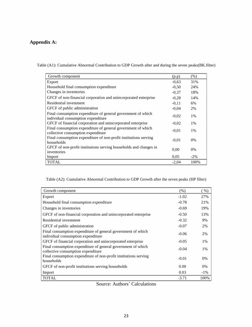
Appendix A:
Table (A1): Cumulative Abnormal Contribution to GDP Growth after and during the seven peaks(BK.filter)
Growth component (p.p) (%)
Export -0,63 31%
Household final consumption expenditure -0,50 24%
Changes in inventories -0,37 18%
GFCF of non-financial corporation and unincorporated enterprise -0,28 14%
Residential investment -0,11 6%
GFCF of public administration -0,04 2%
Final consumption expenditure of general government of which
individual consumption expenditure -0,02 1%
GFCF of financial corporation and unincorporated enterprise -0,02 1%
Final consumption expenditure of general government of which
collective consumption expenditure -0,01 1%
Final consumption expenditure of non-profit institutions serving
households -0,01 0%
GFCF of non-profit institutions serving households and changes in
inventories 0,00 0%
Import 0,05 -2%
TOTAL -2,04 100%
Table (A2): Cumulative Abnormal Contribution to GDP Growth after the seven peaks (HP filter)
Growth component (%) ( %)
Export -1.02 27%
Household final consumption expenditure -0.78 21%
Changes in inventories -0.69 19%
GFCF of non-financial corporation and unincorporated enterprise -0.50 13%
Residential investment -0.32 9%
GFCF of public administration -0.07 2%
Final consumption expenditure of general government of which
individual consumption expenditure -0.06 2%
GFCF of financial corporation and unincorporated enterprise -0.05 1%
Final consumption expenditure of general government of which
collective consumption expenditure -0.04 1%
Final consumption expenditure of non-profit institutions serving
households -0.01 0%
GFCF of non-profit institutions serving households 0.00 0%
Import 0.03 -1%
TOTAL -3.71 100%
Source: Authors’ Calculations