Title Molecular orientation dynamics on the structural rheology indiblock copolymers

Author(s) Yabunaka, Shunsuke; Ohta, Takao

Citation Soft Matter (2013), 9(31): 7479-7488

Issue Date 2013

URL http://hdl.handle.net/2433/190415

Right

This journal is @ The Royal Society of Chemistry 2013; Thisis not the published version. Please cite only the publishedversion. この論文は出版社版でありません。引用の際には出版社版をご確認ご利用ください。

Type Journal Article

Textversion author

Kyoto University

Molecular orientation dynamics on the structural rheology in diblockcopolymers

Shunsuke Yabunaka and Takao Ohta

Received Xth XXXXXXXXXX 20XX, Accepted Xth XXXXXXXXX 20XXFirst published on the web Xth XXXXXXXXXX 200XDOI: 10.1039/b000000x

We formulate a viscoelastic theory of micro-phase separated structures in diblock copolymers in which the local composition iscoupled with the molecular orientation. The linear viscoelastic response is investigated for aligned lamellar structures. Threekinds of complex moduli and viscosities characterizing an incompressible lamellar structure are obtained up to the leading orderof the coupling.

1 Introduction

Diblock copolymers exhibit various periodic microphasestructures in thermal equilibrium1–11. Rheology of thesemesoscopic structures has been investigated to characterizetheir dynamical properties. See, for instance, ref.12 and theearlier references therein. It is mentioned that different phasesshow different rheological properties and hence rheologicalmeasurements are useful to obtain the evidence of the mor-phological transitions13–16.

There are many computational and analytical studies on thestructural rheology of microphase separated diblock copoly-mers. Yoo and Vinals17 considered the effects of anisotropicdiffusion and hydrodynamic interaction. They found thatanisotropy of diffusion influences the grain boundary motionsignificantly. Giupponi et al18 studied gyroid structure in flowby computer simulations of amphiphillic fluids by means ofthe lattice Boltzmann method. They found fluid-like behaviorfor low frequency of viscoelastic response under an oscilla-tory shear flow. Tamate et al19 formulated an analytical theoryof viscoelasticity for interconnected double gyroid structures.They considered concentration variation under shear flow andcalculated the energy dissipation due to the deformation ofinterconnected structures in the weak segregation limit. Thereversible part of the stress tensor which arises from the con-centration variations was calculated by the mode expansion.Their theory relies on the fact that, in the case of a double gy-roid structure, there are two different magnitudes of reciprocallattice vectors22. When the periodic structure is representedby the fundamental reciprocal lattice vectors having only onemagnitude, such as lamellar, hexagonal and body-centered-cubic (BCC) structures, the linear part of loss modulus is ab-sent19.

Department of Physics, Kyoto University, Kyoto 606-8502, Japan. ; E-mail:yabunaka@scphys.kyoto-u.ac.jp

The above fact implies that one needs generally to intro-duce other kinetic variables to describe the structural rheologyof phase-separated diblock copolymers. This is also requiredby another consideration. In an aligned lamellar structure inan incompressible system, there are generally three kinds ofviscosities20. However, it is readily shown by symmetry con-sideration that those viscosities cannot be obtained by a for-mulation which contains only a scalar variable such as a localconcentration. Therefore, although the theories in terms of lo-cal concentration have successfully predicted the equilibriumphase diagram for micro-phase separated states1,6–8, vector ortensor variables are necessary to describe the dynamics, in par-ticular, rheology of mesoscopic periodic structures. We willreturn to this problem in section 5.

In the present paper, we address this problem. To the au-thors’ knowledge, no theories have been available so far to de-rive three kinds of viscosities or three kinds of complex mod-uli for lamellar structure in diblock copolymer melts. It iswell known that diblock copolymer molecules are elongatedin a phase-separated state in the direction parallel to the com-positional gradient21. This occurs even for flexible chains.Therefore we may introduce a local orientational order cou-pled to the local concentration. These are perturbed differ-ently by an external flow and influences the rheological re-sponse of the system. We construct dynamic equations forthe compositional field and the orientational order parameterfield. We analyze these equations by means of the mode ex-pansion in the weak segregation limit and obtain the rheologi-cal response of this system. This approach is related, to someextent, with the theory of smectic liquid crystals. See for ex-ample ref.23 . In this formulation, a phase variable to repre-sent the one-dimensional periodic structure is coupled to theorientational degree of freedom of molecules where, however,complex compliances are not concerned.

Lamellar structure under shear flow becomes unstable since

1–11 | 1

the period tends to be different from the equilibrium one24.There are theoretical studies for both block copolymers25,26

and smectic liquid crystals23,27–29. This nonlinear effect isnot considered in the present paper but we are restricted to thelinear response focusing our attention on the relations betweenseveral kinds of frequency-dependent viscosities.

The organization of the present paper is as follows. In thenext section (section 2), we introduce a kinetic model whichconsists of the local concentration and the local orientationalorder parameter. In section 3, general viscoelastic propertiesare given for lamellar structure under shear flow. The com-plex moduli are calculated up to the first order of the cou-pling between the concentration and the orientation degreesof freedom in section 4. Concluding remarks and discussionare given in section 5. In Appendix A, the macroscopic stresstensor is derived in terms of the local concentration and theorientational field whereas, in Appendix B, some of the de-tails of the viscoelastic response are presented. In AppendixC, the details of the procedure is described to solve the time-evolution equations by the perturbation expansion in terms ofthe coupling strength of the concentration and the orientationalfield, and the strength of the shear rate.

2 Model

We consider A-B type diblock copolymer melts. One of thebasic quantities is the local volume fraction of the A blockdenoted by φ (x). The other is the tensor of the orientationalorder Qi j (x) defined by

Qi j (x) =⟨

mim j −13

δi j

⟩, (1)

where mi is the end-to-end vector for the ith molecule. Notethat this tensor is position-dependent since ⟨· · · ⟩ means a localaverage in a finite volume around a position x, which is muchlarger than the atomic scale and much smaller than the charac-teristic length of deformations of phase separated pattern. Thesimplest expression of the free energy for micro-phase separa-tion in A-B type diblock copolymer is given by

F =∫

dx[

12

L∣∣∣∇φ (x)

∣∣∣2− θ

2φ (x)2 +

g4

φ (x)4 +G(Qi j)

−βQi j(∇iφ)(∇ jφ)+12

C(∇kQi j)(∇kQi j)]

+α2

∫dx

∫dyH (x− y)

[φ (x)− φ

][φ (y)− φ

]. (2)

The repeated indices implies summation. The free energywithout the orientational order parameter was derived by Ohtaand Kawasaki30. The constants L, θ , g, and α are all positivein a microphase separated state. φ is the spatial average of φ .

The term −βQi j(∇iφ)(∇ jφ) represents the coupling betweenthe orientational order parameter and the concentration field.When β > 0 as we assume, each diblock copolymer moleculetends to align in the direction of the composition gradient. Thehomogeneous part of the free energy G(Qi j) for the orienta-tional field takes the simplest form

G(Qi j) =a2

Qi jQi j, (3)

where a > 0 assuming that molecules do not cause sponta-neous alignment. The kernel H (x) in the last term in eqn (2)is defined by

−∇2H (x− y) = δ (x− y) . (4)

This Coulomb-type long range interaction originates from theosmotic incompressibility of diblock copolymer melts30 or, inother words, from the correlation-hole effects31.

In order to derive the time-evolution equations, we employthe variational method developed by Doi for dynamics of var-ious soft matter32. We introduce the local velocity of A and Bcomponents as vA and vB, respectively and define the volumeaverage velocity as

v = φ vA +(1−φ) vB, (5)

and the relative velocity between the two components as

w = vA − vB. (6)

The time evolution equation for the local volume fractionobeys the continuity equation

∂φ∂ t

+ ∇ · (vAφ) = 0. (7)

We employ the variational method to derive the time-evolutionequations. The variational functional is introduced in thepresent problem as

R = Ψ+ F −∫

dx(

p(x)∇ · v+qQii

), (8)

where p is determined by the incompressibility condition∇ · v = 0, and the Lagrange multiplier q is determined by thetraceless condition Qii = 0. The dissipation function Ψ is de-fined by

Ψ =∫

dx[1

2vi jklAi jAkl +

ζi j

2(vA − v)i (vA − v) j

+(Qi j + vm (∇mQi j)+Q jmΩmi +QimΩm j −λi jmnAmn

)×

(Qkl + vn (∇nQkl)+QlnΩnk +QknΩnl −λklmnAmn

)× 1

2Γi jkl

], (9)

2 | 1–11

where ζi j, Γi jkl and λi jkl are constants. We assume that vi jkldepends on Qi j as eqn (21) below. The symmetric velocitygradient tensor Ai j is defined as

Ai j =12

(∂vi

∂x j+

∂v j

∂xi

), (10)

and the antisymmetric one Ωi j as

Ωi j =12

(∂vi

∂x j−

∂v j

∂xi

). (11)

The variations δR/δ vA = 0, δR/δ v = 0 and δR/δ Qi j = 0 to-gether with eqn (7) give us

∂φ∂ t

+ ∇ · (vφ) = ∇i[Di j∇ jδFδφ

], (12)

Qi j + ∇n (vnQi j)+QikΩk j +Q jkΩki −λi jklAkl

= −Γi jkl

(ψkl −

13

δklψmm

), (13)

− ∇ j(vi jklAkl +λkli jψkl +ψikQk j −ψ jkQki − pδi j

)+ φ∇i

δFδφ

− (∇iQkl)ψkl = 0, (14)

where Di j = φ(ζ−1)i j and

Γi jmnΓmnkl =12

(δikδ jl +δilδ jk −

23

δi jδkl

), (15)

ψi j =δF

δQi j= aQi j −C∇2Qi j −β∇iφ∇ jφ . (16)

In eqn (13), the term QikΩk j + Q jkΩki represents the rotationof the molecular orientation in the rotational flow and the term−λi jklAkl represents alignment of molecules in the flow. Wehave assumed that the relative velocity field w does not couplewith the time evolution of the orientational field. This is jus-tified when the dynamical properties of the two components,such as the friction constant, are same in the two blocks.

The coefficients vi jkl and λi jkl have the following properties.First of all, we can assume that vi jkl satisfies

vi jkl = v jikl = vi jlk = v jilk,

viikl = vi jkk = 0, (17)

which follows from Ai j = A ji and Aii = 0. Onsager’s reci-procity is represented as

vi jkl = vkli j. (18)

Similarly we may put

λi jkl = λ jikl = λi jlk = λ jilk, (19)

λiikl = 0,λi jkk = 0, (20)

which follows from Ai j = A ji,Qi j = Q ji and Aii = Qii = 0. Weexpand vi jkl in terms of Qi j as33

vi jkl = v1

(δikδ jl +δ jkδil −

23

δi jδkl

)+v2

(δikQ jl +δ jkQil +δ jlQik +δilQ jk

−43

δi jQkl −43

δklQi j

)+O(Q2

i j). (21)

It will be shown in Appendix C that this expansion turns outto be an expansion in terms of the coupling strength β .

Hereafter we set the coefficients λi jkl , Γi jkl , Di j to beisotropic constants as λδikδ jl , Γδikδ jl , Dδi j although thesemay be anisotropic generally and functions of Qi j and φ . Thiscan be justified in the weak segregation limit where the com-position variation and the orientational order is weak over thespace. From the above relations, the time evolution equations(12) and (13) are given, respectively, by

∂φ∂ t

+ ∇ · (vφ) = D∇2 δFδφ

, (22)

Qi j +∇n (vnQi j)+QikΩk j +Q jkΩki −λAi j

= −Γ[aQi j −C∇2Qi j −β ((∇iφ)(∇ jφ)

− 13

δi j(∇kφ)(∇kφ))]

, (23)

where we assume that λ > 0 such that molecules tend to ex-tend to the flow direction.

The total macroscopic stress tensor consists of two parts

Σi j ≡1V

∫dxσi j =

1V

∫dxσ r

i j +1V

∫dxσd

i j, (24)

with V the system volume. The reversible part can be derivedfrom the free energy (2) as

Σri j =

1V

∫dxσ r

i j

= − 1V

∫dx

[L(∇ jφ (x))(∇iφ (x))

+ C (∇ jQkl (x))(∇iQkl (x))]

+α2V

∫dx

∫dy[∇iH (x− y)](x j − y j)φ (x)φ (y)

+βV

∫dx[Qik (∇kφ (x))(∇ jφ (x))

+ Q jk (∇kφ (x))(∇iφ (x))]+λV

∫dxψi j. (25)

When the orientational order parameter is absent, this agreeswith that derived by Kawasaki and Ohta34. We describe the

1–11 | 3

detail of the derivation of (25) in Appendix A. The dissipativepart of the stress tensor is given from eqn (14) and (21) by

Σdi j =

1V

∫dxσd

i j =1V

∫dx

(vi jklAkl

)= 2v1Ai j +2v2

(Q jlAil +QilA jl −

23

δi jQklAkl

)+ O(Q2

i j). (26)

The incompressibility condition Aii = 0 has been used.

3 Theory of linear viscoelastic response forlamellar structures

In this section we investigate the linear viscoelastic responsefor lamellar structures under an oscillatory shear flow given by

vi (xi, t) = γi j (t)x j, (27)

withγi j (t) = γ0i j sinωt. (28)

Here γ0i j is a constant second rank tensor. There might befluctuations of the local velocity field around the shear flow(27) due to deformations of the microphase separated struc-ture. But this hydrodynamic effects can be neglected in thecase of block copolymer melts except for extremely low fre-quency regime. It has been argued in ref19 that when the meltviscosity is proportional to the molecular weight35, the hy-drodynamic effects are not important in the weak segregationregime. Actually many viscoelastic theories ignore the hydro-dynamic effects. See, e.g., refs36,37. Moreover, experimentaldata for block copolymer melts are found to be fitted by theRouse model without hydrodynamic effects38.

We consider the viscoelastic response of the macroscopicstress tensor (25) for an aligned lamellar structure. Before car-rying out detailed calculations, we discuss the general proper-ties. The normal unit vector n is defined such that it is parallelto the fundamental reciprocal vector of the lamellar structurein the absence of shear flows. Without loss of generality, wemay assume that n is parallel to the x axis. Up to linear orderof the shear strength, we note that there are three contributionsby symmetry argument

Σi j =12

(γ0i j + γ0 ji

)(G′

1 (ω)sinωt +G′′1 (ω)cosωt

)+

12

(γ0kl + γ0lk)(G′

2 (ω)sinωt +G′′2 (ω)cosωt

)×

(δik (n jnl)+δ jk (ninl)−

23

δi jnknl

)+

(G′

3 (ω)sinωt +G′′3 (ω)cosωt

)×

(nin j −

13

δi j

)nknlγ0kl . (29)

We may write down each component explicitly.

Σxx =(

G′1 (ω)+

43

G′2 (ω)+

23

G′3 (ω)

)× γ0xx sinωt

+(

G′′1 (ω)+

43

G′′2 (ω)+

23

G′′3 (ω)

)× γ0xx cosωt, (30)

Σyy = G′1 (ω)γ0yy sinωt +G′′

1 (ω)γ0yy cosωt

+(−2

3G′

2 (ω)− 13

G′3 (ω)

)γ0xx sinωt

+(−2

3G′′

2 (ω)− 13

G′′3 (ω)

)γ0xx cosωt, (31)

Σxy =(G′

1 (ω)+G′2 (ω)

) 12

(γ0xy + γ0yx)sinωt

+(G′′

1 (ω)+G′′2 (ω)

) 12

(γ0xy + γ0yx)cosωt, (32)

Σyz =(G′

1 (ω)) 1

2(γ0yz + γ0zy)sinωt

+(G′′

1 (ω)) 1

2(γ0yz + γ0zy)cosωt, (33)

where only the traceless part is taken into consideration be-cause the trace part corresponds to the pressure, and the to-tal pressure is determined by the incompressibility condition.We may define similarly the functions Gr

i (ω) and Gdi (ω),

(i = 1,2,3) for the reversible parts and the dissipative part ofthe stress tensor, respectively.

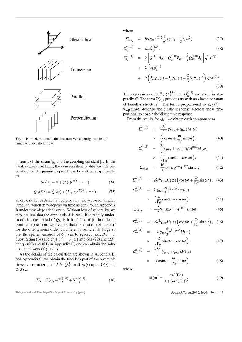
In the case of an oriented lamellar structure, there are threefundamental configurations for applying shear flow as shownin Fig. 1. In the perpendicular configuration, the normal oflamellae is perpendicular to both the flow direction and thevelocity gradient direction. In the parallel configuration, thenormal is parallel to the velocity gradient direction but per-pendicular to the flow direction. In the transverse configura-tion, the normal is parallel to the flow direction but perpendic-ular to the velocity gradient direction. It is readily shown thatwhen the lamellar structure is periodic along the x axis, thestress in the flow direction for the parallel and the transverseconfiguration is given by Σxy = Σyx whereas the stress for theperpendicular configuration is given by Σyz.

It is also remarked that three kinds of complex moduli ineqn (29) is consistent with the fact that there are three vis-coelastic constants for lamellar structures under the incom-pressibility condition39.

4 Explicit form of the stress tensor

Now we discuss the response of the stress tensor. In orderto evaluate the reversible part of the stress tensor given by eqn(25), we solve eqn (22) and (23) by the perturbation expansion

4 | 1–11

Shear Flow

Transverse

Parallel

Perpendicular

Fig. 1 Parallel, perpendicular and transverse configurations oflamellae under shear flow.

in terms of the strain γi j and the coupling constant β . In theweak segregation limit, the concentration profile and the ori-entational order parameter profile can be written, respectively,as

φ (r, t) = φ +(A(t)eiq·r + c.c.), (34)

Qi j (r, t) = Qi j(t)+(Bi j(t)e2iq·r + c.c.), (35)

where q is the fundamental reciprocal lattice vector for alignedlamellae, which may depend on time as eqn (76) in AppendixB under time-dependent strain. Without loss of generality, wemay assume that the amplitude A is real. It is readily under-stood that the period of Qi j is half of that of φ . In order toavoid complication, we assume that the elastic coefficient Cfor the orientational order parameter is sufficiently large sothat the spatial variation of Qi j can be ignored, i.e., Bi j = 0.Substituting (34) and Qi j (r, t) = Qi j(t) into eqn (22) and (23),or eqn (80) and (81) in Appendix C, one can obtain the solu-tions in powers of γ and β .

As the details of the calculation are shown in Appendix B,and Appendix C, we obtain the traceless part of the reversiblestress tensor in terms of A(1), Q(1)

i j , and γi j (t) up to O(γ) andO(β ) as

Σri j = Σr

el,i j +Σr(1,0)i j +βΣr(1,1)

i j , (36)

where

Σrel,i j = 8αγxxA(0)2 1

q4 (qiq j −13

δi jq2), (37)

Σr(1,0)i j = λaQ(1,0)

i j , (38)

Σr(1,1)i j = 2

[Q(1,0)

ix δ jx +Q(1,0)jx δix −

23

Q(1,0)xx δi j

]q2A(0)2

+ λ[aQ(1,1)

i j

+ 2(

δixγx j (t)+δ jxγxi (t)−23

δi jγxx (t))

q2A(0)2].

(39)

The expressions of A(0), Q(1,0)i j and Q(1,1)

i j are given in Ap-pendix C. The term Σr

el,i j provides us with an elastic constantof lamellar structure. The terms proportional to γαβ (t) =γ0αβ sinωt describe the elastic response whereas those pro-portional to cosωt the dissipative response.

From the results for Qi j, we obtain each component as

Σr(1,0)xy =

aλ 2

2(γ0xy + γ0yx)M(ω)

×(

cosωt +ωΓa

sinωt)

, (40)

Σr(1,1)xy =

λ2

(γ0xy + γ0yx)4q2A(0)2M(ω)

×( ω

Γasinωt + cosωt

). (41)

Σrel,xx =

163

γ0xxαq−4A(0)2 sinωt, (42)

Σr(1,0)xx = aλ 2γ0xxM(ω)

(cosωt +

ωΓa

sinωt)

, (43)

Σr(1,1)xx = λγ0xx

163

q2A(0)2M(ω)

×( ω

Γasinωt + cosωt

). (44)

Σrel,yy = −8

3γ0xxαq−4

∣∣∣A(0)∣∣∣2

sinωt, (45)

Σr(1,0)yy = aλ 2γ0yyM(ω)

(cosωt +

ωΓa

sinωt)

, (46)

Σr(1,1)yy = −λγ0xx

83

q2A(0)2M(ω)

×( ω

Γasinωt + cosωt

). (47)

Σr(1,0)yz =

aλ 2

2(γ0yz + γ0zy)M(ω)

×(

cosωt +ωΓa

sinωt)

. (48)

where

M(ω) =ω/(Γa)

1+(ω/(Γa))2 (49)

1–11 | 5

We have dropped some terms by noting that q2 =√

α/L +O

(β 2

)as eqn (88) in Appendix C. It is noted that only the

symmetric part of the velocity gradient contributes to the vis-coelastic response, because the antisymmetric part representsthe uniform rotation of the system. Eqn (42) for Σr

el,xx gives usthe elastic response due to the deformation of lamellar struc-tures, which exists even when the coupling between the orien-tational order parameter and the concentration field is absent.Σr(1,0)

i j represents the viscoelastic response of molecular align-ment due to the flow and this contribution exists even whenthere is no microphase separated structure. The viscoelasticresponse Σr(1,1)

i j which is proportional to A(0)2 arises from themicrophase separated structures and the coupling between theorientational order parameter and the concentration field. Thecharacteristic relaxation rate relevant to Σr(1,0)

i j and Σr(1,1)i j is

Γa, which is the relaxation frequency of the orientational or-der parameter. If we take the Rouse dynamics for individualchains, this relaxation rate is proportional to N−2 with N themolecular weight35. When ω is much larger (smaller) thanΓa, these responses reduce to the elastic (viscous) response.This situation would change if we take into account the secondorder contribution of the coupling β , because it may containthe relaxation rate of composition fluctuations.

Finally the above results for the macroscopic reversiblestress tensor can be rewritten in the form of eqn (29) by setting

G′r1 (ω) = aλ 2 ω

ΓaM(ω), (50)

G′′r1 (ω) = aλ 2M(ω), (51)

G′r2 (ω) = 4λβq2

∣∣∣A(0)∣∣∣2 ω

ΓaM(ω), (52)

G′′r2 (ω) = 4λβq2

∣∣∣A(0)∣∣∣2

M(ω), (53)

and

G′r3 (ω) = 8αq−4

∣∣∣A(0)∣∣∣2

, (54)

G′′r3 (ω) = 0. (55)

Therefore, we obtain a Maxwell-type complex moduli Gr1 and

Gr2 up to the linear order of the coupling constant β . We note

that in the limit ω → 0, only the storage modulus G′r3 (ω) re-

mains finite. Yamada and Ohta40 calculated the elastic con-stants of several microphase separated structures. The elasticresponse given by (54) agrees with that for lamellar structureobtained by them. There are generally two kinds of elasticconstants for lamellar structure or smectic A liquid crystals41.One is the dilation and the other is the bending of the layerstructure. In our theory we have obtained only the dilation ofthe layer structure since the bending energy is represented bythe higher spatial derivative.

Similarly, the macroscopic dissipative stress tensor can bederived from eqn (26) and the expressions of Qi j in AppendixC. The final results are given by

G′d1 (ω) = G

′d2 (ω) = G

′d3 (ω) = 0, (56)

G′′d1 (ω) =

(2v1 −

43

Sv2

)ω, (57)

G′′d2 (ω) = 2v2Sω, (58)

G′′d3 (ω) = 0. (59)

where S = 2(β/a)q2A(0)2.

5 Concluding remarks and discussion

In this paper, we have formulated a linear vsicoelastic the-ory for aligned lamellar structures in microphase separateddiblock copolymers. We have applied the mode expansionmethod in the weak segregation limit, and evaluated the lin-ear viscoelastic response up to the first order of the couplingconstant β between the composition gradient and the molecu-lar orientation.

We can evaluate the viscosities of lamellar structure fromthe theory developed here. It is well known that there arethree kinds of viscosities for incompressible fluids with uniax-ial symmetry17,20. The macroscopic dissipative stress tensorcan be written as

ΣDi j = α1nin jnknlAkl +α4Ai j +α5nkniAk j +α6nkn jAki

−13

δi j (α1 +α5 +α6)nknlAkl , (60)

with α5 = α6. From eqn (58) and (59), and taking the ω → 0limit of the loss moduli (51) and (53), we obtain

α1 = 0, (61)

α4 = 2(v1 −23

Sv2)+λ 2

Γ, (62)

α5 = α6 = 2v2S +2λSΓ

. (63)

In the disordered state at high temperature, we may put S = 0so that α5 = α6 = 0 and α4 = 2ν1. Comparing this with eqn(62), one notes that the viscosity α4 for the perpendicular con-figuration decreases in the lamellar phase provided that thecoefficient ν2 which appears in eqn (21) is positive. Sincethe loss modulus for the parallel configuration in the low fre-quency limit is given by α4 +α5, this is larger than that for theperpendicular configuration since the coefficient λ in eqn (23)is positive as we have assumed.

6 | 1–11

As long as we have noticed, the complex moduli (50)-(59) and the viscosities (61)-(63) are new results. Therehave been no theories to formulate these linear viscoelasticquantities for lamellar structures in diblock copolymer melts.There are some rheological experiments for aligned lamellarblock copolymers. Koppi et al42 carried out dynamical me-chanical measurements for the three lamellar configurationsshown in Fig. 1 in sheared diblock copolymer melts. Athigher frequency, the dynamical elastic moduli as well as thefrequency-dependent viscosities are not distinguishable for thethree configurations whereas these take different values forsmaller frequencies. For example, the viscosity for perpendic-ular lamellae is smaller than that of parallel lamellae consis-tent qualitatively with our results mentioned above. However,their data for the perpendicular configuration become differ-ent from those for the transverse configuration. Theoreticallythe shear stress for these two configurations should be equalto each other due to the symmetry Σxy = Σyx. This discrep-ancy at low frequency may be originated from some nonlin-ear and/or nonequilibirium effects. Shear alignment and rhe-ological measurements have also been conducted for lamellarPolystyrene-Polyisoprene block copolymers by Patel et al43

where the loss modulus for parallel lamellae near the order-disorder transition temperature is larger than that of perpen-dicular ones in the double logarithmic plot as a function of fre-quency scaled by the shift factor. This trend is again consistentwith our results. A quantitative comparison seems impossi-ble because of the large contrast in the viscoelastic propertiesbetween the styrene and isoprene blocks in the experimentswhile our theory assumes dynamical symmetry for the twoblocks. We note that there is another experiment for lamellarPolystyrene-Polyisoprene block copolymers44 in which theloss modulus of parallel configuration is smaller than that ofperpendicular configuration. However, the experiment wascarried out at 120 C which is not close to the order-disordertransition 164 C and the data are outside applicability of thepresent theory in the weak segregation. Hahn et al38 have car-ried out experiments of lamellar block copolymers minimizingdefect density. Their data for the best aligned sample of per-pendicular configuration indicate that G′ ∝ ω2 and G′′ ∝ ω forthe low frequency regime consistent with the present results.

The present study implies that one has to choose care-fully the relevant dynamical variables for microphase sepa-rated structures. As mentioned in the Introduction, the equilib-rium phase diagram has been obtained successfully by meanfield theories essentially in terms of local concentrations1,6–8.The static elastic theory has also been formulated based on thesimilar theories40,45. Dynamics of phase ordering and mor-phological transitions have been studied extensively by thetime-evolution equations for the local concentrations22,46–48.However, the viscoelastic properties cannot be obtained prop-erly only by the local concentrations. This can be seen from

the reversible part of the macroscopic stress tensor (25) whichis given in the absence of the variable Qi j by

1V

∫dxσ r

i j = −∑q

qiq j

[L− α

q4

]φqφ−q, (64)

where φq is the Fourier component of φ (r) with q the funda-mental reciprocal vectors. The strain dependence of qi as (76)in Appendix B gives us the elastic constants. The dissipationdue to deformation arises from the relaxation of the concen-tration φq. It is obvious that, by expanding φq in terms of theshear rate, the stress (64) can produce a term in the form of theα1 term in eqn (60) provided that q is proportional to n. How-ever, it is impossible to obtain other terms in eqn (60). In thepresent study, we have considered the orientational degrees offreedom and have shown that they contribute to the dissipativepart of the viscoelastic response in lamellar structure.

6 Acknowledgements

One of the authors (T.O.) would like to thank Dr. A. Menzelfor valuable discussions at the early stage of this study. Thiswork was supported by the JSPS Core-to-Core Program ”In-ternational research network for non-equilibrium dynamics ofsoft matter” and the Grant-in-Aid for the Global COE Program”The Next Generation of Physics, Spun from Universality andEmergence” from the Ministry of Education, Culture, Sports,Science and Technology (MEXT) of Japan. One of the authors(S. Y.) acknowledges support from JSPS (Grant No. 241799),and the other (T. O.) from JSPS (Grand No. 23540449 and24244063).

A Derivation of the reversible macroscopicstress tensor

We derive the macroscopic stress tensor Σri j by calculating the

free energy deviation by the following infinitesimal uniformdeformation u (x)

r = x+ u (x) , (65)

ui (x) = (∇ jui)x j. (66)

Here we assume that (∇ jui) is constant in space. Throughoutthis paper, we will use the coordinate ri for the moving frame,and xi for the laboratory frame.

1–11 | 7

The variables φ and Qi j are transformed as

φ ′ (r) = φ (x) , (67)

Q′i j (r) = Qi j (x)+

12

Qik (∇ku j −∇ juk)

+12

Q jk (∇kui −∇iuk)

+12

λi jkl (∇kul +∇luk)

= Qi j (x)+(QikWk j +Q jkWki

)+λi jklCkl . (68)

Here we have defined the symmetric deviation gradient tensorCi j and the antisymmetric deviation gradient tensor Wi j as

Ci j =12

(∇iu j +∇ jui) , (69)

Wi j =12

(∇iu j −∇ jui) . (70)

The gradient term is transformed by

∇i = ∇′i +(∇iu j)∇′

j. (71)

Here the prime symbols indicate the derivative in the coordi-nate system r. The free energy deviation in the first order of uis calculated as follows.

δF =∫

dr f(

φ ′ (r) ,Q′i j (r)

)−

∫dx f

(φ (x) ,Qi j (x)

)= 2β

∫dxQik (∇kφ (x))(∇ jφ (x))∇iu j (x)

+∫

dx(ψk jQki∇iu j −ψkiQk j∇iu j

)+

∫dxψklλkli j∇iu j

− L∫

dx(∇ jφ (x))(∇iφ (x))∇iu j (x)

− C∫

dx(∇ jQkl (x))(∇iQkl (x))∇iu j (x)

+α2

∫dx

∫dy

[(∇iH (x− y))ui (x)− (∇iH (x− y))ui (y)]× φ (x)φ (y) . (72)

In this derivation, we have employed eqn (67) and (68), andthe following relations under the incompressibility condition

− L∫

dx(∇i∇ jφ (x))(∇iφ (x))u j (x)

=L2

∫dx(∇iφ (x))(∇iφ (x))∇ ju j (x) = 0, (73)

2β∫

dxQi j (∇ jφ (x))(∇i∇kφ (x))uk (x)

+β∫

dx(∇kQi j)(∇ jφ (x))(∇iφ (x))uk (x)

= −β∫

dxQi j (∇ jφ (x))(∇iφ (x))∇kuk (x) = 0. (74)

By substituting the expression of ψi j given by eqn (16), wecan further simplify this expression as

δF = β∫

dx[Qik (∇kφ (x))(∇ jφ (x))

+ Q jk (∇kφ (x))(∇iφ (x))]∇iu j

+∫

dxψklλkli j∇iu j

− L∫

dx(∇ jφ (x))(∇iφ (x))∇iu j

− C∫

dx(∇ jQkl (x))(∇iQkl (x))∇iu j

+α2

∫dx

∫dy

[(∇ jH (x− y))(xi − yi)∇iu j]φ (x)φ (y) . (75)

From this, we may define the stress tensor as∫

dxσ ri j∇iu j and

obtain the formula given by eqn (25).

B Calculation of the viscoelastic response

In this Appendix, we describe the details of calculation of theviscoelastic response. First we express the reversible stresstensor in terms of the amplitude A and Qi j up to the first orderof the strain γ . We define the time dependent wave number as

qi (t) = q0i − γ ji (t)q0 j, (76)

where q0 is the fundamental reciprocal lattice vector of un-deformed lamellae. Substituting eqn (34), (35), and (82) inAppendix C into eqn (25), we obtain

Σri j = [−2Lqi (t)q j (t)+2α

qi (t)q j (t)

q(t)4 ]A(0)2

+ 2βqk (t) [Q(1)ik (t)q j (t)+ Q(1)

jk (t)qi (t)]A(0)2

+ λ[aQ(1)

i j

+ 2β (qiγk j (t)qk +q jγki (t)qk −23

δi jqkγlk (t)ql)A(0)2

− 4β (qiq j −13

δi jq2)(A(0)A(1))]+O

(γ2,β 2) . (77)

8 | 1–11

Using eqn (76), this can be evaluated as

Σri j = 2

(L− α

q4

)A(0)2 (δixγx j (t)+δ jxγxi (t))

+ 8αγxxqiq j

q4 A(0)2 +2β[Q(1)

ix δ jx + Q(1)jx δix

]q2A(0)2

+ λ[aQ(1)

i j

+ 2β(

δixγx j (t)+δ jxγxi (t)−23

δi jγxx (t))

q2A(0)2

− 4β(

δixδ jx −13

δi j

)q2

(A(0)A(1)

)]+ O

(γ2,β 2) . (78)

The first term on the right hand side vanishes because of theequilibrium condition q2 =

√α/L as eqn (88).

C Perturbation expansions

Here we obtain the solutions of the time-evolution equationscalculated by the perturbation expansion. We introduce thenew coordinate r which moves with the flow

ri (t) = xi − γi j (t)x j. (79)

In the moving frame, the time evolution equations are given as

∂φ∂ t

= D∇2[−L∇2φ −θφ +gφ 3 +2β∇i(Qi j∇ jφ)

]− Dα

(φ − φ

), (80)

∂Qi j

∂ t+ QikΩk j +Q jkΩki −λi jklAkl

= −Γ[aQi j −β (∇iφ)(∇ jφ)+

β3

(∇iφ)2δi j

]+ C∇2Qi j, (81)

where

∇i ≡ ∇i − γ ji∇ j. (82)

The operator ∇i contained in Ωki and Akl should not be re-placed by ∇i since it acts on the local velocity. See AppendixA.

In order to solve eqn (80) and (81) in the weak segregationlimit, we put φ (r, t) and Qi j (r, t) as eqn (34) and (35), respec-tively and make an expansion of the amplitudes in powers ofthe strain γ;

A = A(0) +A(1) +O(γ2) , (83)

Qi j = Q(0)i j + Q(1)

i j +O(γ2) . (84)

The zeroth order solutions are given as follows. From eqn (81)we have

aQ(0)i j (r)−β

(∇iφ (0) (r)∇ jφ (0) (r)− 1

3

∣∣∣∇φ (0)∣∣∣2

δi j

)= 0.

(85)By substituting eqn (83), the amplitude Q(0)

i j is given by

Q(0)i j =

2βa

q2∣∣∣A(0)

∣∣∣2(

δixδ jx −13

δi j

). (86)

From eqn (80) and (83), we obtain

−q2(

Lq2A(0) −θA(0) +3gA(0)∣∣∣A(0)

∣∣∣2+3gφ 2A(0)

)− αA(0) = 0, (87)

where O(β 2) terms are omitted. The magnitude of the wavenumber q is determined from the minimization of the free en-ergy. By substituting eqn (86) and (83) into eqn (2), we obtain

∂F∂q

= L−αq−4 +O(β 2) = 0, (88)

and hence q2 =√

α/L.At the first order of the shear strength γ , equations for the

amplitude A(1) and Q(1)i j are given, respectively, by

dA(1)

dt= −3gDq2

∣∣∣A(0)∣∣∣2

A(1) +2Dβq4A(0)Q(1)xx

+ O(β 2) , (89)

dQ(1)xx

dt= −ΓaQ(1)

xx +83

Γβq2A(0)A(1) +λγ0xxω cosωt

− 83

Γβq2∣∣∣A(0)

∣∣∣2γ0xx sinωt, (90)

dQ(1)yy

dt= −ΓaQ(1)

yy − 43

Γβq2A(0)A(1) +λγ0yyω cosωt

+43

Γβq2∣∣∣A(0)

∣∣∣2γ0xx sinωt, (91)

dQ(1)xy

dt= −ΓaQ(1)

xy

− βq2∣∣∣A(0)

∣∣∣2 (Γsinωt +

ωa

cosωt)

(γ0xy − γ0yx)

+(

12

λω cosωt −Γβ sinωtq2∣∣∣A(0)

∣∣∣2)

× (γ0xy + γ0yx) , (92)

dQ(1)yz

dt= −ΓaQ(1)

yz +12

λ (γ0yz + γ0zy)ω cosωt. (93)

We can solve these linear equations exactly, but the solutionis complicated. Instead we expand these equations in terms of

1–11 | 9

the coupling strength β as

Q(1)i j = Q(1,0)

i j +β Q(1,1)i j +O

(γβ 2) , (94)

A(1) = A(1,0) +βA(1,1) +O(γβ 2) . (95)

The lowest order contributions Q(1,0)xx and A(1,0) satisfy

ddt

(Q(1,0)

xx

A(1,0)

)=

(−Γa 0

0 −ΓA

)(Q(1,0)

xx

A(1,0)

)

+(

λω cosωt0

)γ0xx, (96)

where

ΓA = 3gDq2A(0)2. (97)

The asymptotic solutions for t →∞ are given by A(1,0) = 0 and

Q(1,0)xx =

λωΓa

N(ω)(

cosωt +ωΓa

sinωt)

γ0xx, (98)

whereN(ω) =

1

1+(ω/Γa)2 . (99)

Similarly we obtain

Q(1,1)xx = − 8

3aγ0xxq2A(0)2N(ω)

×(

sinωt − ωΓa

cosωt)

, (100)

Q(1,0)yy =

λωΓa

γ0yyN(ω)

×(

cosωt +ωΓa

sinωt)

, (101)

Q(1,1)yy =

43a

q2A(0)2γ0xxN(ω)

×(

sinωt − ωΓa

cosωt)

, (102)

Q(1,0)xy =

ωΓa

λ2

(γ0xy + γ0yx)N(ω)

×(

cosωt +ωΓa

sinωt)

, (103)

Q(1,1)xy = −(γ0xy + γ0yx)

q2

aA(0)2N(ω)

×(

sinωt − ωΓa

cosωt)

− (γ0xy − γ0yx)q2

aA(0)2 sinωt, (104)

Q(1)yz =

ωΓa

λ2

(γ0yz + γ0zy)N(ω)

×(

cosωt +ωΓa

sinωt)

. (105)

It is noted that, since A(1,0) = 0, there are no contributions toQ(1,0)

i j and Q(1,1)i j from A(1), and that Q(1)

yz has no contributionfrom the spatial variation of the concentration as can be seenfrom eqn. (93).

References

1 M. W. Matsen and M. Schick, Phys. Rev. Lett., 1994, 72,2660.

2 S. Forster, A. K. Khandpur, J. Zhao, F. S. Bates, I. W.Hamley, A. J. Ryan and W. Bras, Macromolecules, 1994,27, 6922.

3 A. K. Khandpur, S. Foerster, F. S. Bates, I. W. Hamley, A.J. Ryan, W. Bras, K. Almdal and K. Mortensen, Macro-molecules, 1995, 28, 8796.

4 M. W. Matsen and F. S. Bates, Macromolecules, 1996, 29,1091.

5 M. W. Matsen and F. S. Bates, Journal of ChemicalPhysics, 1997, 106, 2436.

6 E. W. Cochran, C. J. Garcia-Cervera and G. H. Fredrick-son, Macromolecules, 2006, 39, 2449.

7 C. A. Tyler and D. C. Morse, Phys. Rev. Lett., 2005, 94,208302.

8 K. Yamada, M. Nonomura and T. Ohta, Journal ofPhysics-Condensed Matter, 2006, 18, L421.

9 A. Ranjan and D. C. Morse, Phys. Rev. E, 2006, 74,011803.

10 M. Takenaka, T. Wakada, S. Akasaka, S. Nishitsuji, K.Saijo, H. Shimizu, M. I. Kim and H. Hasegawa, Macro-molecules, 2007, 40, 4399.

11 B. Miao and R. A. Wickham, J. Chem. Phys., 2008, 128,054902.

12 M. B. Kossuth, D. C. Morse and F. S. Bates, J. Rheol.,1999, 43, 167.

13 M. E. Vigild, K. Almdal, K. Mortensen, I. W. Hamley, J.P. A. Fairclough and A. J. Ryan, Macromolecules, 1998,31, 5702.

14 C.-Y. Wang and T. P. Lodge, Macromolecules, 2002, 35,6997.

15 G. Floudas, R. Ulrich and U. Wiesner, J. Chem. Phys.,1999, 110, 652.

16 M. F. Schulz, F. S. Bates, K. Almdal and K. Mortensen,Phys. Rev. Lett., 1994, 73, 86.

17 C. D. Yoo and J. Vinals, Macromolecules, 2012, 45, 4848.18 G. Giupponi, J. Harting and P. V. Coveney, Europhys.

Lett., 2006, 73, 533.19 R. Tamate, K. Yamada, J. Vinals, and T. Ohta, J. Phys.

Soc. Jpn., 2008, 77, 034802.20 J. L. Ericksen, J. Arch. Rational Mech. Anal., 1959, 4, 231.21 Y. Matsushita, K. Mori, Y. Mogi, R. Saguchi, I. Noda, M.

10 | 1–11

Nagasawa, T. Chang, C. Glinka and C. C. Han, Macro-molecules 1990, 23, 4317.

22 K. Yamada, M. Nonomura and T. Ohta, Macromolecules,2004, 37, 5762.

23 I. W. Stewart and F. Stewart, J. Phys.: Condens. Matter,2009, 21, 465101.

24 D. R. M. Williams and F. C. MacKintosh, Macro-molecules, 1994, 27, 7677.

25 G. Fredrickson, J. Rheol., 1994, 38, 1045.26 F. Drolet, P. Chen, and J. Vinals, Macromolecules, 1999,

32, 8603.27 G. K. Auernhammer, H. R. Brand and H. Pleiner, Rheo-

logica Acta, 2000, 39, 215.28 G. K. Auernhammer, H. R. Brand and H. Pleiner, Phys.

Rev. E, 2002, 66, 061707.29 A. S. Wunenburger, A. Colin, T. Colin and D. Roux, Eur.

Phys. J. E, 2000, 2, 277.30 T. Ohta and K. Kawasaki Macromolecules, 1986, 19,

2621.31 P. G. de Gennes, Scaling concepts in polymer physics, Cor-

nell University Press, New York 1979.32 M. Doi, J. Phys. Condens. Matter, 2011, 23, 284118.33 H. Pleiner, M. Liu, and H.R. Brand, IMA Proceedings in

Mathematics and its Applications, Springer, New York,2005, 141, 99.

34 K. Kawasaki and T. Ohta, Physica A, 1983, 118, 17535 M. Doi and S. F. Edwards, The Theory of Polymer Dynam-

ics, Oxford University Press, London, 1986.36 K. Kawasaki and A. Onuki, Phys. Rev. A, 1990, 42, R3664.37 M. Rubinstein and S. P. Obukhov, Macromolecules, 2001,

34 8701.38 H. Hahn, J. H. Lee, N. P. Balsara, B. A. Garetz and H.

Watanabe, Macromolecules, 1993, 26 1740.39 P. C. Martin, and O. Parodi, and P. S. Pershan, Phys. Rev.

A, 1972, 6, 2401.40 K. Yamada and T. Ohta, Europhys. Lett., 2006, 73, 614.41 P. G. de Gennes and J. Prost, The Physics of Liquid Crys-

tals, Clarendon Press, Oxford, 1993, 2nd ed.42 K. A. Koppi, M. Tirrell, F. S. Bates, K. Almdal and R. H.

Colby, J. Phys. II France, 1992, 2, 1941.43 S. S. Patel, R. G. Larson, K. I. Winey and H. Watanabe,

Macromolecules, 1995, 28 4313.44 V. K. Gupta, R. Krishnamoorti, J. A. Kornfield and S. D.

Smith, Macromolecules, 1996, 29 1359.45 C. A. Tyler and D. C. Morse, Macromolecules, 2003, 36

8184.46 M. Bahiana and Y. Oono, Phys. Rev. A, 1990, 41, 6763.47 T. Kawakatsu, Statistical Physics of Polymers, Springer-

Verlag, Heidelberg, 2004.48 J. G. E. M. Fraaije, J. Chem. Phys., 1993, 99, 9202.

1–11 | 11