Scilab  tutorial  –  satellite    orbit  around  the  earth  

1. Express  the  physics  problem      The  problem  is  based  on  the  universal  law  of  gravitation:    

𝐹 =  −𝐺 ∗𝑚 ∗𝑀𝑟 ! ∗

𝑟𝑟  

   We  write  down  Newton’s  third  law  of  motion  in  an  earth-­‐centred  referential:      

𝑚 ∗ 𝑥 =  −𝐺 ∗ !∗!( !!!!!)!

∗ 𝑥  

𝑚 ∗ 𝑦 =  −𝐺 ∗ !∗!( !!!!!)!

∗ 𝑦  

   

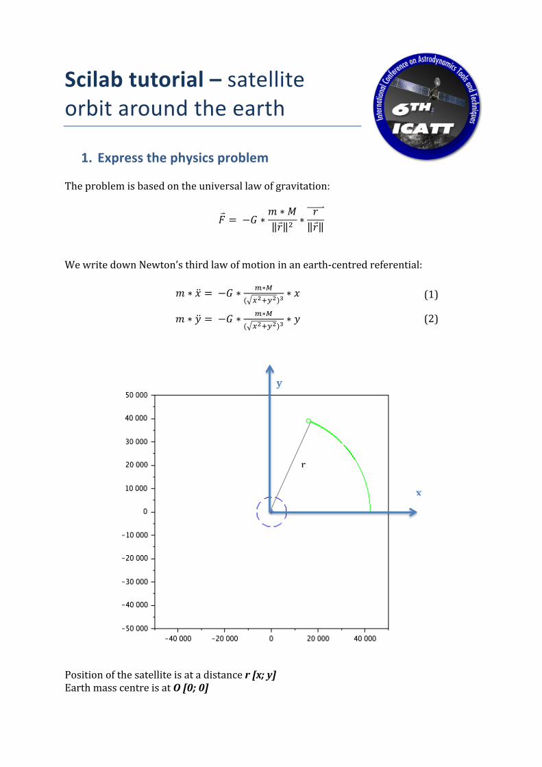
   Position  of  the  satellite  is  at  a  distance  r  [x;  y]  Earth  mass  centre  is  at  O  [0;  0]  

x  

y  

r  

(1)  

(2)  

Constants  of  the  problem:  Gravitational  constant  𝐺   =  6.67  ×  10!!!  𝑚!𝑘𝑔!!𝑠!!  Mass  of  the  earth  𝑀   =  5.98  ×  10!"  𝑘𝑔  Radius  of  the  Earth  𝑟!"#$! =  6.38  ×  10!  𝑚      

2. Translate  your  problem  into  Scilab    Scilab   is   a   matrix-­‐based   language.   Instead   of   expressing   the   system   as   set   of   4  independent  equations  (along  the  x  and  y  axis,  for  position  and  speed),  we  describe  it  as  a  single  matrix  equation,  of  dimension  4x4:      This  method  is  a  classical  trick  to  switch  from  a  second  order  scalar  differential  equation  to  a  first  order  matrix  differential  equation.    

𝑢   = 𝐴.𝑢      

with  𝐴 =

0 0 1 00 0 0 1

𝑐/𝑟! 0 0 00 𝑐/𝑟! 0 0

,  𝑢 =

𝑥𝑦𝑥𝑦  

 To  simplify  the  equation,  we  define  the  variable  𝑐 =  −𝐺 ∗𝑀  

 Open  scinotes  with  edit  myEarthRotation.sci  Define  the  skeleton  of  the  function:    

function udot=f(t, u) G = 6.67D-11; //Gravitational constant M = 5.98D24; //Mass of the Earth c = -G * M; r_earth = 6.378E6; //radius of the Earth r = sqrt(u(1)^2 + u(2)^2); // Write the relationhsip between udot and u if r < r_earth then udot = [0 0 0 0]'; else A = [[0 0 1 0]; [0 0 0 1]; [c/r^3 0 0 0]; [0 c/r^3 0 0]]; udot = A*u; end endfunction

 The  condition  defined  by  the  distance  r  of  the  satellite  with  the  centre  of  earth  stops  the  simulation  if  it’s  colliding  with  earth’s  surface.    

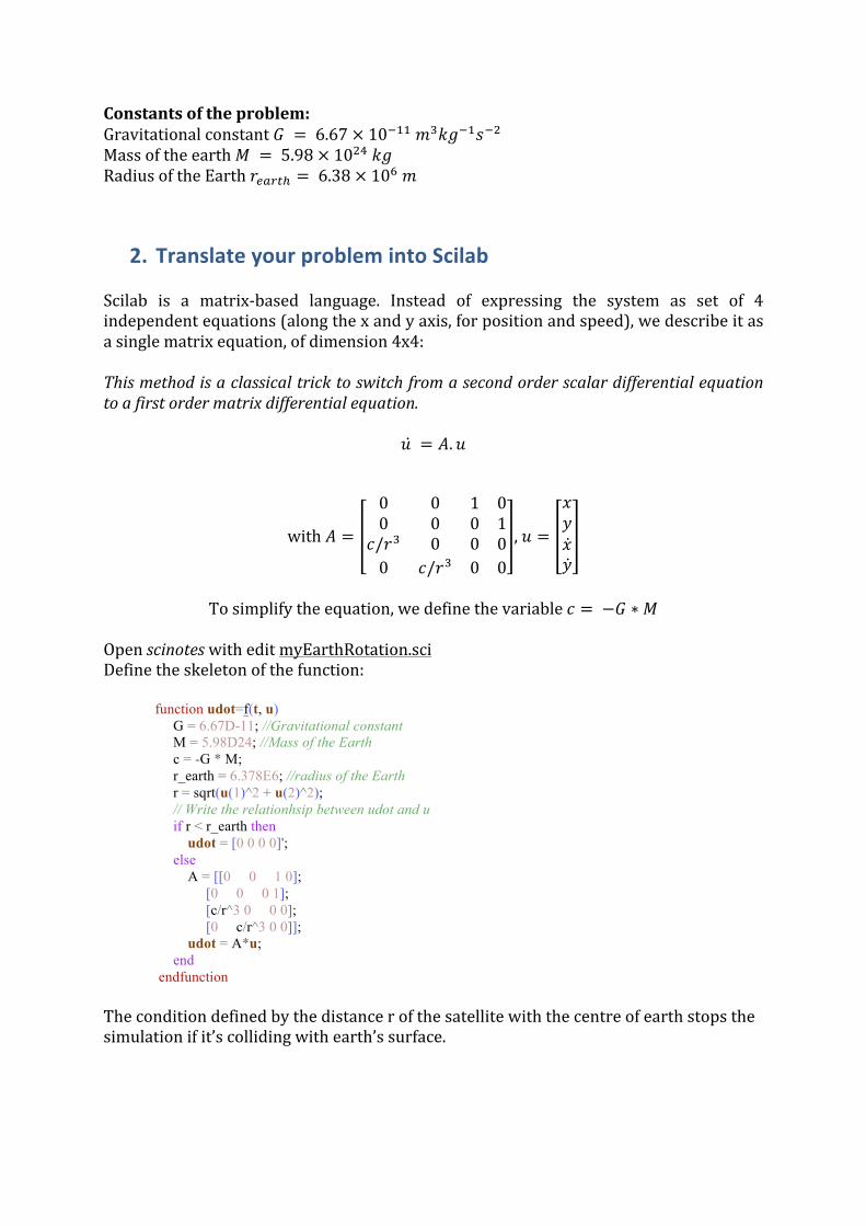
 Try  out  the  final  script  with  the  following  initial  conditions  in  speed  and  altitude:  

geo_alt = 35784; // in kms geo_speed = 1074; // in m/s simulation_time = 24; // in hours U = earthrotation(geo_alt, geo_speed, simulation_time);

 

3. Compute  the  results  and  create  a  visual  animation    With  this  function,  we  go  to  the  core  of  the  problem.      

function U=earthrotation(altitude, v_init, hours) // altitude given in km // v_init is a vector [vx; vy] given in m/s // hours is the number of hours for the simulation r_earth = 6.378E6; altitude = altitude * 1000; U0 = [r_earth + altitude; 0; 0; v_init]; t = 0:10:(3600*hours); // simulation time, one point every 10 seconds U = ode(U0, 0, t, f); // Draw the earth in blue angle = 0:0.01:2*%pi; x_earth = 6378 * cos(angle); y_earth = 6378 * sin(angle); fig = scf(); a = gca(); a.isoview = "on"; plot(x_earth, y_earth, 'b--'); plot(0, 0, 'b+'); // Draw the trajectory computed comet(U(1,:)/1000, U(2,:)/1000, "colors", 3); endfunction  

 The  resolution  of  the  ordinary  differential  equation  (ODE)  is  computed  with  the  Scilab  function  ode.        

ode  solves  Ordinary  Different  Equations  defined  by:    

𝑦   = 𝑓(𝑡,𝑦)  where  y  is  a  real  vector  or  matrix  

 The  simplest  call  of  ode  is:  y  =  ode(y0,t0,t,f)  where  y0  is  the  vector  of  initial  conditions,  t0  is  the  initial  time,  t  is  the  vector  of  times  at  which  the  solution  y  is  computed  and  y  is  matrix  of  solution  vectors  y=[y(t(1)),y(t(2)),...].    To  go  further  in  numerical  analysis,  find  out  more  about  the  solvers:  Ordinary  Differential  Equations  with  Scilab,  WATS  Lectures,  Université  de  Saint-­‐Louis,  G.  Sallet,  2004    

Complete  script    // // Scilab ( http://www.scilab.org/ ) - This file is part of Scilab // Copyright (C) 2015-2015 - Scilab Enterprises - Pierre-Aimé Agnel // // This file must be used under the terms of the CeCILL. // This source file is licensed as described in the file COPYING, which // you should have received as part of this distribution. The terms // are also available at // http://www.cecill.info/licences/Licence_CeCILL_V2.1-en.txt // function udot=f(t, u) G = 6.67D-11; //Gravitational constant M = 5.98D24; //Mass of the Earth c = -G * M; r_earth = 6.378E6; //radius of the Earth r = sqrt(u(1)^2 + u(2)^2); // Write the relationhsip between udot and u if r < r_earth then udot = [0 0 0 0]'; else A = [[0 0 1 0]; [0 0 0 1]; [c/r^3 0 0 0]; [0 c/r^3 0 0]]; udot = A*u; end endfunction function U=earthrotation(altitude, v_init, hours) // altitude given in km // v_init is a vector [vx; vy] given in m/s // hours is the number of hours for the simulation r_earth = 6.378E6; altitude = altitude * 1000; U0 = [r_earth + altitude; 0; 0; v_init]; t = 0:10:(3600*hours); // simulation time, one point every 10 seconds U = ode(U0, 0, t, f);

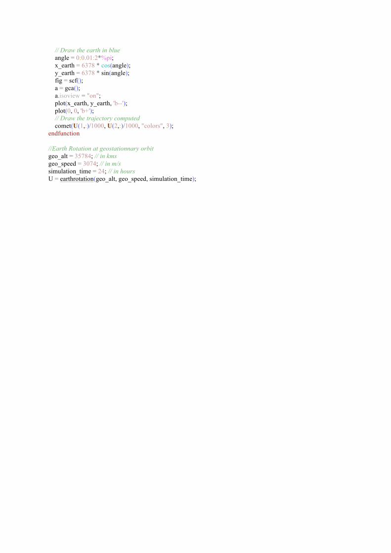
// Draw the earth in blue angle = 0:0.01:2*%pi; x_earth = 6378 * cos(angle); y_earth = 6378 * sin(angle); fig = scf(); a = gca(); a.isoview = "on"; plot(x_earth, y_earth, 'b--'); plot(0, 0, 'b+'); // Draw the trajectory computed comet(U(1,:)/1000, U(2,:)/1000, "colors", 3); endfunction //Earth Rotation at geostationnary orbit geo_alt = 35784; // in kms geo_speed = 3074; // in m/s simulation_time = 24; // in hours U = earthrotation(geo_alt, geo_speed, simulation_time);