universidad catÓlica andrÉs bello...
TRANSCRIPT

Desarrollo de un Sistema de Apoyo Docente Basado en Tecnología de Información para la Enseñanza de las Telecomunicaciones
Página 1
UNIVERSIDAD CATÓLICA ANDRÉS BELLO
VICERRECTORADO ACADÉMICO ESTUDIOS DE POSTGRADO
ÁREA DE GERENCIA Postgrado en Sistemas de Información
Trabajo Especial de Grado
DESARROLLO DE UN SISTEMA DE APOYO DOCENTE BASADO EN TECNOLOGIA DE INFORMACION PARA LA ENSENANZA DE LAS
TELECOMUNICACIONES
Presentado por Barrios José Javier
Para optar al título de Especialista en Sistemas de Información
Asesor Ing. Manuel Gaspar
Caracas 31/10/2007

Desarrollo de un Sistema de Apoyo Docente Basado en Tecnología de Información para la Enseñanza de las Telecomunicaciones
Página 2
DEDICATORIA A mis padres y hermanas. A mis amigos y compañeros de trabajo. A mi niña linda.

Desarrollo de un Sistema de Apoyo Docente Basado en Tecnología de Información para la Enseñanza de las Telecomunicaciones
Página 3
AGRADECIMIENTOS A los profesores Nincola Buonanno, Maria Cristi Stefanelli y Trina de Pérez por su apoyo para la realización de este trabajo. Al profesor Manuel Gaspar por su guía en la realización de este trabajo.
Desarrollo de un Sistema de Apoyo Docente Basado en Tecnología de Información para la Enseñanza de las Telecomunicaciones
Página 4
RESUMEN
La carrera de Ingeniería de Telecomunicaciones tiene 5 años desde su
creación en la Universidad Católica Andrés Bello.
La carrera se fundamenta en la estructura que tienen las diferentes
escuelas que conforman la Facultad de Ingeniería, el Plan de Estudios
comprende diez semestres de formación Básica y Profesional.
Actualmente el proceso de enseñanza-aprendizaje de las materias
Señales y sistemas I, comunicaciones I y comunicaciones II es de gran dificultad
para los docentes asignados a estas asignaturas, dificultad basada en la
complejidad práctica y matemática de los conceptos asociados a esta materias.
El propósito de este proyecto es desarrollar un sistema de información
basado en un simulador programable que apoye y mejore el proceso de
enseñanza-aprendizaje de las telecomunicaciones, específicamente en las
materias antes mencionadas.
El sistema desarrollado esta enmarcado dentro de los diferentes enfoques
educativos (conductismo y constructivismo), tomando algunos aspectos de los
mismos, que mejor se adecuen al contexto de enseñanza-aprendizaje.
Palabras claves: Sistemas de información basados en simuladores
programables, análisis y diseño e implantación de sistemas, telecomunicaciones
en la academia.

Desarrollo de un Sistema de Apoyo Docente Basado en Tecnología de Información para la Enseñanza de las Telecomunicaciones
Página 5
INDICE DE CONTENIDO INTRODUCCIÓN …………………………………………………………... 8 CAPITULO I PLANTEAMIENTO DEL TEMA ……………………………. 10
1.2 Antecedentes ………………………………………………………….. 12 1.3 Objetivo General ............................................................................ 13 1.3 .1Objetivos Específicos ………………………………………………… 13 1.4.1 Importancia de la simulación en el contexto educativo …………… 14 1.4.2 Los sistemas de telecomunicaciones ………………………………. 15 1.4.3 Productividad ………………………………………………………….. 16 1.5 ALCANCE ……………………………………………………………… 17 CAPITULO II MARCO TEORICO ………………………………………... 21 2.2 Relación de las TIC con los Sistemas de Información………………. 21 2.3 Recursos de información……………………………………………….. 28 2.4 Tipos de modulación analógica………………………………………… 33 2.5 Tipos de modulación digital…………………………………………….. 39 2.6 Técnicas Didácticas……………………………………………………. 46 2.7 Tipos de aprendizaje explicados por los diferentes enfoques ……… 47 2.8 Simulación Didáctica…………………………………………………… 49 2.9 Ambientes Colaborativos de Aprendizaje…………………………….. 49 2.10 Elementos básicos para propiciar el aprendizaje colaborativo ….. 50 2.11 Interdependencia positiva…………………………………………….. 50 2.12 Contribución individual ……………………………………………….. 51 2.13 Habilidades personales y de grupo …………………………………. 51 2.14 Ambientes colaborativos soportados con tecnología informática .. 51 2.15 Entornos de aprendizaje basados en simulaciones informáticas .. 52 2.16 Lenguaje de programación con orientación a la ciencia y tecnología Matlab …………………………………………………………….
53
46 CAPITULO III MARCO METODOLOGICO ………………………………. 57 46 3.1 Características metodológicas del levantamiento de información…. 57 3.2 Problema………………………………………………………………… 58 3.3 Tipo de investigación…………………………………………………… 60 3.4 Diseño del trabajo especial de grado ………………………………… 60 3.5 Instrumentos……………………………………………………………. 61 3.6 Procedimientos…………………………………………………………. 61 3.7 Instrumentos para el levantamiento de información…………………. 63

Desarrollo de un Sistema de Apoyo Docente Basado en Tecnología de Información para la Enseñanza de las Telecomunicaciones
Página 6
3.8 Análisis de los datos……………………………………………………. 64 3.9 Análisis y Diseño del Sistema …………………………………………. 65 CAPITULO IV DESARROLLO DE LA PROPUESTA…………………… 67 4.1 Análisis de la situación actual………………………………………….. 67 4.2 Propuesta del modelo de Sistema de Información basado en simulador programable………………………………………………………
73
4.2.1 Entradas del sistema..………………………………………………… 73 4.2.2 Análisis conceptual del Sistema de Apoyo a la Enseñanza de las Telecomunicaciones (SAET)……………………………………………….
75
4.2.3 Requerimientos del sistema SAET ………………………………….. 84 4.2.4 Carta estructurada de procesos…................................................. 84 4.2.5 Estructura General del sistema SAET………………………………. 85 4.2.6 Entradas, procesos y salidas del sistema SAET ………………….. 86 4.2.7 Programación y pruebas ……………………………………………... 111 CAPITULO V CONCLUSIONES ………………………………………...... 123 5.1 RECOMENDACIONES…………………………………………………. 124 REFERENCIAS BIBLIOGRAFICAS………………………………………. 125
ÍNDICE DE TABLAS
Tabla 1: Aplicaciones y parámetros de la codificación.………………….. 43 Tabla 2: Conocimientos requeridos en las materias seleccionadas para el desarrollo del sistema SAET………………………………………..
75
Tabla 3: Esquema de entradas, procesos y salidas del modulo de señales y sistemas……………………………………………………………
93
Tabla 4: Esquema de entradas, procesos y salidas del modulo de comunicaciones analógicas …………………………………………………
100
Tabla # 5: Esquema de entradas, procesos y salidas del modulo de comunicaciones digitales.………………………………
110

Desarrollo de un Sistema de Apoyo Docente Basado en Tecnología de Información para la Enseñanza de las Telecomunicaciones
Página 7
ÍNDICE DE FIGURAS Figura1: Diagrama en bloques de la estructura de un sistema de información .…………………………………………………………………..
29
Figura 2: Diagrama en bloques de un sistema de comunicaciones……. 30 Figura 3: traslación del mensaje a través de la modulación.……………. 33 Figura 4: Representación en forma de onda de la señal muestreada…... 40 Figura 5: Señal muestreada de forma natural…………………………….. 41 Figura 6: Representación de una señal muestreada y retenida…........... 41 Figura 7: Representación de la cuantificación de una señal……………. 42 Figura 8: Representación de la codificación de una señal……………… 42 Figura 9: Análisis de simulaciones didácticas…………………………….. 49 Figura 10: Implicaciones de un aprendizaje basado en simulaciones…. 52 Figura 11: Receptor de radio AM………………………………………………………….. 53 Figura 12: Pantalla principal del software MATLAB………………………………. 55 Figura 13: Código fuente del software MATLAB………………………….. 56 Figura 14: Diagrama de bloques del modelo lineal secuencial…………. 66 Figura 15: diagrama de flujo de datos. Nivel 0……………………………. 76 Figura 16: Diagrama de Flujo de Datos. Nivel 1………………………….. 79 Figura 17: Diagrama de Flujo de Datos. Nivel 1…………………………………… 81 Figura 18: Diagrama de Flujo de Datos. Nivel 1………………………….. 83
Desarrollo de un Sistema de Apoyo Docente Basado en Tecnología de Información para la Enseñanza de las Telecomunicaciones
Página 8
Figura 19: Carta estructurada de procesos………………………………………. 84 Figura 21: Estructura del sistema propuesto …………………………….. 85 Figura 22: Pantalla inicial sistema SAET………………………………………………. 111 Figura 23: Modulo de señales y sistemas del sistema SAET…………… 112 Figura 24: Modulo de señales y sistemas generación, del sistema SAET. 112 Figura 25: Modulo de señales y sistemas operaciones, del sistema SAET…………………………………………………………………………...
113
Figura 26: Modulo de señales y sistemas otras operaciones, del sistema SAET…………………………………………………………………
114
Figura 27: Modulo de señales y sistemas filtraje, del sistema SAET…... 114 Figura 28: Modulo de comunicaciones analógicas del sistema SAET…. 115 Figura 29: Modulo de comunicaciones analógicas generación del mensaje, del sistema SAET………………………………………………….
115
Figura 30: Modulo de comunicaciones analógicas modulación, del sistema SAET…………………………………………………………………
116
Figura 31: Modulo de comunicaciones analógicas modulación caracterización del canal, del sistema SAET………………………………
116
Figura 32: Modulo de comunicaciones analógicas detección de la señal, del sistema SAET……………………………………………………..
117
Figura 33: Modulo de comunicaciones digitales del sistema SAET……. 117 Figura 34: Modulo de comunicaciones digitales generación del mensaje, del sistema SAET…………………………………………………
118
Figura 35: Modulo de comunicaciones digitales modulación PCM, del sistema SAET…………………………………………………………………
118
Figura 36: Modulo de comunicaciones digitales compansión, del

Desarrollo de un Sistema de Apoyo Docente Basado en Tecnología de Información para la Enseñanza de las Telecomunicaciones
Página 9
sistema SAET………………………………………………………………… 119 Figura 37: modulo de comunicaciones digitales codificación PCM, del sistema SAET…………………………………………………………………
119
Figura 38: Modulo de comunicaciones digitales modulación, del sistema SAET…………………………………………………………………
120
Figura 39: Modulo de comunicaciones digitales modulación caracterización del canal, del sistema SAET……………………………..
120
Figura 40: Modulo de comunicaciones digitales detección de la señal, del sistema SAET……………………………………………………………..
121
Figura 41: Modulo de comunicaciones digitales curvas de PE del sistema SAET…………………………………………………………………
121
Figura 42: Modulo de comunicaciones digitales modulación multinivel, del sistema SAET……………………………………………………………..
122
Figura 43: Modulo de comunicaciones digitales modulación multinivel curvas de PE, del sistema SAET…………………………………………..
122
ÍNDICE DE GRAFICAS
Grafica 1: Representación en forma de onda de la señal mensaje…….. 35 Grafica 2: Representación en forma de onda de la señal portadora.…... 36 Grafica 3: Representación en forma de onda de la señal modulada en amplitud………………………………………………………………………..
36
Grafica 4: Representación en forma de onda de la señal modulada en doble banda lateral……………………………………………………………
37
Grafica 5: Representación en forma de onda de la señal modulada en banda lateral única..…………………………………………………………..
38

Desarrollo de un Sistema de Apoyo Docente Basado en Tecnología de Información para la Enseñanza de las Telecomunicaciones
Página 10
Grafica 6: Representación en forma de onda de la señal modulada en banda lateral única……………………………………………………………
39
Grafica 7: Representación en forma de onda de la señal modulada por conmutación de amplitud…………………………………………………….
44
Grafica 8: Representación en forma de onda de la señal modulada por conmutación de de frecuencia………………………………………………
45
Grafica 9: Representación en forma de onda de la señal modulada por conmutación de de fase……………………………………………………...
46

Desarrollo de un Sistema de Apoyo Docente Basado en Tecnología de Información para la Enseñanza de las Telecomunicaciones
Página 11
INTRODUCCIÓN
Las tecnologías de Información basadas en simuladores programables
constituyen herramientas que apoyan el trabajo docente. Trabajo docente que
consiste en impartir conocimientos en áreas especificas a los futuros
profesionales universitarios.
Los Sistemas de información de apoyo docente facilitan el proceso de
enseñanza-aprendizaje teórico y práctico, ya que la representación simulada de
un fenómeno específico se asemeja en gran proporción a la realidad, por otro
lado las instituciones universitarias en ocasiones no cuentan con recursos
económicos para implementar laboratorios con equipamiento específico para
reforzar los conocimientos teóricos obtenidos. .
Para la elaboración de este trabajo se tomó como caso de Estudio tópicos
de asignaturas de la carrera de Ingeniería de Telecomunicaciones de la UCAB,
en conjunto con los profesores del área.
El esquema de este trabajo especial de grado está compuesto por cinco
capítulos. En el capítulo I, se presenta el planteamiento del tema, antecedentes,
alcances, objetivo general y objetivos específicos.
En el capítulo II, se desarrolla el marco teórico, en el que se presentan los
conceptos que enmarcan el desarrollo del trabajo especial de grado.
En el capítulo III, se encuentra el marco metodológico, donde se indica las
características metodológicas empleadas para el desarrollo del trabajo.

Desarrollo de un Sistema de Apoyo Docente Basado en Tecnología de Información para la Enseñanza de las Telecomunicaciones
Página 12
En el capítulo IV, se desarrolla el proyecto, a través del análisis de la
situación actual, la propuesta para el desarrollo del sistema de información
académico basado en un simulador programable, los requerimientos del sistema
y la programación y pruebas del mismo.
En el capítulo V, se presentan conclusiones y recomendaciones
generadas por el proyecto.
Por ultimo se presentan las referencias bibliográficas consultadas y los
anexos.

Desarrollo de un Sistema de Apoyo Docente Basado en Tecnología de Información para la Enseñanza de las Telecomunicaciones
Página 13
CAPITULO I 1.1 PLANTEAMIENTO DEL TEMA. En la actualidad la convergencia de las tecnologías de información y
comunicaciones (TIC), incrementa la eficiencia organizacional con la
funcionalidad de implementar mejores sistemas de comunicación para el
procesamiento y el transporte de la información, por lo cual estos sistemas se
complementan uno al otro.
Por otro lado, los sistemas de información son ayudados por sistemas de
comunicaciones, dentro del proceso de gestión de sistemas de información, por
lo cual de no existir las tecnologías de comunicaciones la información no seria
accesible a cada ente de una organización.
En el ámbito académico las tecnologías de la información y comunicación (TIC)
han provocado profundos cambios sociales y culturales además de cambios
económicos. Uno de los sectores más impactados directamente es el sistema
educativo pues la nueva generación de las TIC ha transformado el papel o rol
social del aprendizaje. La universidad como institución formal responsable de la
formación y capacitación de los recursos humanos, debe responder a las
interrogantes y desafíos de la cultura y la tecnología que le ha tocado vivir, así
como a las necesidades que las nuevas generaciones plantean1.
Por otro lado es importante destacar el crecimiento de las telecomunicaciones y
la informática a nivel mundial hasta el punto de crear carreras específicas en las
universidades con los objetivos de formar recurso humano en estas áreas de
conocimiento.
Dibut, L. Valdés, G., Arteaga, H. & all (1998). Las nuevas tecnologías de la información y la comunicación
como mediadoras del proceso enseñanza-aprendizaje. http://tecnologiaedu.us.es/edutec/paginas/61.html.
Consultado enero 2007.

Desarrollo de un Sistema de Apoyo Docente Basado en Tecnología de Información para la Enseñanza de las Telecomunicaciones
Página 14
Dentro del proceso de formación de un ingeniero de telecomunicaciones los
participantes estudian asignaturas relacionados con el área, los cuales se
pueden clasificar en:
Circuitos y sistemas electrónicos.
Análisis de señales.
Comunicaciones analógicas.
Comunicaciones digitales.
Sistemas microondas.
Sistemas de fibra óptica.
Antenas y propagación de ondas.
Procesamiento y transmisión de datos.
Telemática.
Sistemas de comunicaciones móviles.
Los procesos o fenómenos que involucran estos tópicos se pueden explicar
mediante modelos matemáticos y modelos físicos, específicamente en las áreas
de análisis de señales, comunicaciones analógicas y digitales, por lo cual se
requiere de una descripción teórica previa, además de una sesión practica
posterior con la finalidad de que el participante comprenda los procesos
relacionados con el tema que se explica.
El proceso de enseñanza aplicado en el diseño instruccional de las materias
antes mencionadas, es de tipo formativo, ya que los participantes serán
capacitados y entrenados para analizar, comprender y evaluar fenómenos
relacionados con el área de la ingeniería de telecomunicaciones. En algunos
casos, el proceso de enseñanza-aprendizaje se dificulta ya que existen temas
relacionados con las materias a tratar que no son de fácil comprensión, ya que

Desarrollo de un Sistema de Apoyo Docente Basado en Tecnología de Información para la Enseñanza de las Telecomunicaciones
Página 15
poseen alto nivel de abstracción y alto contenido matemático que de llevarse a
un modelo físico requerían de equipos y dispositivos costosos.
En los laboratorios de formación en el campo de ingeniería de
telecomunicaciones, se mezclan procesos que se pueden representar:
a) De forma física (practicas de laboratorio con circuitos integrados y
discretos o módulos prácticos)
b) Con herramientas de simulación (tecnología de información basada en
simuladores programables aplicada a telecomunicaciones).
Esto contribuye con el análisis y comprensión de procesos físicos complicados
para su desarrollo practico (por el costo de los componentes y equipos de
medición); dichas herramientas tienen un alto índice de confiabilidad ya que se
pueden programar situaciones muy semejantes a la realidad.
Con este trabajo se pretende desarrollar una herramienta para el apoyo del
proceso de enseñanza-aprendizaje en el campo de las telecomunicaciones
analógicas y digitales, basado en un simulador programable (SIBSP).
1.2 ANTECEDENTES
Desarrollo y Evaluación de un ambiente de aprendizaje que incluya TIC,
basadas en Web, en los cursos de comunicaciones eléctricas de la USB. Prof.
Trina Adrián de Pérez. Prof. María Cristi Stefanelli, Prof. María Elizabeth
González y Prof. Emill Morgado. Proyecto presentado ante el Decanato de
Investigaciones USB.

Desarrollo de un Sistema de Apoyo Docente Basado en Tecnología de Información para la Enseñanza de las Telecomunicaciones
Página 16
1.3 OBJETIVO GENERAL
Elaborar un programa informático de simulación que apoye el proceso de
enseñanza-aprendizaje en el campo de las telecomunicaciones.
1.3.1 Objetivos Específicos
Establecer las estrategias que enmarcaran el proceso de enseñanza-
aprendizaje en el campo de las telecomunicaciones.
Recopilar los contenidos relevantes en las diferentes cátedras de la
carrera de ingeniería de telecomunicaciones.
Desarrollar el sistema de computación para la simulación de señales
analógicas y digitales relacionado con los contenidos seleccionados.
Representar los resultados de la simulación de manera fácil y
comprensible y que a su vez permita la interacción de forma amigable y
didáctica con el usuario.
1.4 JUSTIFICACION
Se comenzará por abordar tres tópicos importantes:
La importancia de la simulación de señales en el contexto educativo.
Los sistemas de telecomunicaciones.
Productividad.

Desarrollo de un Sistema de Apoyo Docente Basado en Tecnología de Información para la Enseñanza de las Telecomunicaciones
Página 17
De los cuales primero se desarrollará la importancia de la simulación en el
ámbito educativo, luego los de telecomunicaciones y por ultimo los sistemas de
información, este último se analizara desde el punto de vista laboral
(organizacional), luego se llevara al ámbito académico
1.4.1 Importancia de la simulación en el contexto educativo
La incorporación de simulaciones informáticas a la enseñanza de las
telecomunicaciones debe entenderse como un problema tecnológico y didáctico.
Si bien es verdad que se necesitan equipos y aplicaciones informáticas
sofisticadas, también lo es que la ausencia de estrategias adecuadas para hacer
útil esa tecnología en el aprendizaje de conceptos y en el desarrollo de
habilidades propias del trabajo científico, puede dificultar su consolidación futura
en las aulas. Por ello, tienen interés las investigaciones orientadas a poner de
manifiesto las condiciones óptimas en que debe desarrollarse una enseñanza
apoyada en el uso de simulaciones informáticas.
Para el diseño de una instrucción educativa con esas características se debe
tener en cuenta aportes de diferentes campos tales como: teorías generales del
aprendizaje, teorías del diseño de la instrucción, investigaciones en la didáctica
de las ciencias, investigaciones en entornos educativos multimedia,
investigaciones sobre espacios colaborativos de aprendizaje. De su análisis,
pueden deducirse una serie de directrices que han de orientar el diseño de
entornos de aprendizaje basados en simulaciones informáticas, por lo cual:
Las simulaciones deben ser usadas para promover un aprendizaje
basado en la investigación de los alumnos.
En un proceso de enseñanza/aprendizaje apoyado en simulaciones los
alumnos y profesores tienen que jugar un papel activo

Desarrollo de un Sistema de Apoyo Docente Basado en Tecnología de Información para la Enseñanza de las Telecomunicaciones
Página 18
Las actividad investigadora de los alumnos y de los profesores se
potencia en un ambiente colaborativo.
El uso de las simulaciones debe ser coherente con un planteamiento
constructivista para el proceso de enseñanza/aprendizaje
En muchas ocasiones, la dificultad para comprender un fenómeno físico se
asocia a la complejidad matemática que le rodea (este es el caso de los
sistemas de telecomunicaciones). Sin embargo habría que recordar que son dos
dimensiones (comprensión física y explicación matemática), que no tienen
porqué coincidir. Por lo cual, el uso de las simulaciones supone un valor
agregado a las tareas educativas dirigidas a la representación de conceptos
abstractos o al control de la escala de tiempos, permitiendo mejorar el proceso
habitual de enseñanza (que comienza con el tratamiento matemático) a la vez de
mostrar el fenómeno a través de una animación gráfica o representación
tridimensional2.
Por otro lado se ejecutaran nuevas estrategias para el proceso de enseñanza
ayudadas con la tecnología de información facilitando el aprendizaje de manera
de aumentar la calidad de la formación del recurso humano sobre la plataforma
de las teorías de aprendizaje que serán descritas a lo largo del desarrollo técnico
del trabajo.
1.4.2 Los sistemas de telecomunicaciones
Es difícil imaginar como seria la vida moderna sin el fácil acceso a medios de
comunicación confiables, económicos y eficientes. En la actualidad los sistemas
de comunicaciones se hallan dondequiera que se transmita información de un
punto a otro, el teléfono, la radio y la televisión son ejemplos de esto.
2. Zamarro, J.M.; Martín, E.; Esquembre, F. y Härtel, H (1998) Unidades didácticas en Física utilizando simulaciones interactivas controladas desde ficheros HTML. Comunicación IV Congreso RIBIE, Brasilia. http://www.niee.ufrgs.br/ribie98/TRABALHOS/100.PDF . consultado abril 2007.
Desarrollo de un Sistema de Apoyo Docente Basado en Tecnología de Información para la Enseñanza de las Telecomunicaciones
Página 19
Los sistemas de comunicaciones actuales son el soporte de procesos de
negocio, procesos de alta gerencia, industria, banca y son necesarios para la
divulgación de información al público.
En el ámbito académico de Venezuela la Universidad Católica Andrés Bello es
la pionera en la creación y desarrollo de una carrera de ingeniería especifica del
área de las telecomunicaciones, con lo cual se destaca la importancia del
sistema propuesto, ya que se pretende mejorar la calidad academica del recurso
humano en formación.
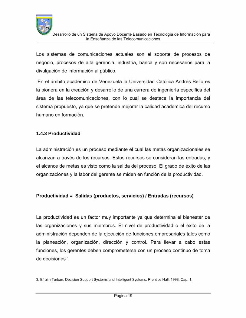
1.4.3 Productividad
La administración es un proceso mediante el cual las metas organizacionales se
alcanzan a través de los recursos. Estos recursos se consideran las entradas, y
el alcance de metas es visto como la salida del proceso. El grado de éxito de las
organizaciones y la labor del gerente se miden en función de la productividad.
Productividad = Salidas (productos, servicios) / Entradas (recursos)
La productividad es un factor muy importante ya que determina el bienestar de
las organizaciones y sus miembros. El nivel de productividad o el éxito de la
administración dependen de la ejecución de funciones empresariales tales como
la planeación, organización, dirección y control. Para llevar a cabo estas
funciones, los gerentes deben comprometerse con un proceso continuo de toma
de decisiones3.
3. Efraim Turban, Decision Support Systems and Intelligent Systems, Prentice Hall, 1998. Cap. 1.

Desarrollo de un Sistema de Apoyo Docente Basado en Tecnología de Información para la Enseñanza de las Telecomunicaciones
Página 20
Desde el punto de vista académico se puede presentar ciertas analogías con lo
explicado anteriormente:
El concepto de productividad se describe en entradas (recursos) y salidas
(productos, servicios), que se pueden llevar al campo académico relacionando la
productividad con la formación de recurso humano en el área de las
telecomunicaciones; en efecto las entradas están representadas por el recurso
humano (profesores-estudiantes) y recursos tecnológicos (computadoras,
software y laboratorios). Las salidas vienen conformadas por las actividades de
formación integral del ingeniero de telecomunicaciones, con sólidos
conocimientos de los sistemas de telecomunicaciones3.
1.5 ALCANCE
Para esta propuesta se desarrollará un sistema de información academico
basado en herramientas de simulación programables para el apoyo a la
enseñanza de las telecomunicaciones, el sistema tendrá como nombre Sistema
de Apoyo a la Enseñanza de las Telecomunicaciones (SAET).
El lenguaje de programación con orientación a las ciencias y tecnologia a utilizar
es el MatLab (Laboratorio de Matrices) desarrollado por los proyectos LINPACK
y EISPACK. Hoy en día Matlab incorpora bibliotecas LINPACK y BLAS, el cual
será descrito de forma funcional en el marco teórico.
3. Efraim Turban, Decision Support Systems and Intelligent Systems, Prentice Hall, 1998. Cap. 1.

Desarrollo de un Sistema de Apoyo Docente Basado en Tecnología de Información para la Enseñanza de las Telecomunicaciones
Página 21
Como la herramienta a desarrollar ayudará al proceso de enseñanza de las
telecomunicaciones es importante destacar que solo se hará una descripción de
la metodología didáctica que utilizará el docente a la hora de utilizarla, esta
metodología estará basada en los procesos didácticos empleados para el
aprendizaje (El Conductismo, el Cognitivismo y el Constructivismo), donde solo
se establecerá con cual de estos procesos será impartida la clase con la ayuda
de la herramienta.
En función de que el desarrollo técnico es un sistema de aplicación informática,
solo se van a describir los procesos de análisis, diseño e implementación del
sistema.
Desde la perspectiva organizacional el análisis y diseño de sistemas se refiere al
proceso de examinar una situación de la organización con la intención de
mejorarla mediante nuevos procedimientos y métodos4.
El análisis corresponde al proceso que sirve para recopilar e interpretar los
hechos, diagnosticar problemas y utilizar estos hechos a fin de mejorar el
sistema5.
Considerando el hecho de que el análisis es la respuesta directa al “que” del
sistema y lo descompone, de un todo en partes mas pequeñas6. El análisis que
se llevara a cabo para este trabajo esta determinado por:
Levantamiento de información.
Definición de los procesos.
4. James A. Senn, Análisis y diseno de sistemas de información. McGaw-Hill. 1987. 619 Pág. 5. James A. Senn, Análisis y diseno de sistemas de información. McGaw-Hill. 1987. 619 Pág. 6. Guía de clases de la materia Análisis y Diseno de sistemas de información del profesor Jesús Ramírez

Desarrollo de un Sistema de Apoyo Docente Basado en Tecnología de Información para la Enseñanza de las Telecomunicaciones
Página 22
El diseño de sistemas es el proceso de planificación de un nuevo sistema dentro
de la organización para reemplazar o complementar uno existente5.
El diseño responde a “cómo” hacer el sistema y lo sintetiza en partes. Por lo
cual para el diseno del sistema propuesto se ejecutará:
La planificación y elaboración del sistema que comprende los pasos de
entrada proceso salida.
Desarrollo de los elementos que establecen como el sistema cumplirá los
requerimientos identificados en el análisis.
Ejecutar el diseño lógico y el diseño físico del sistema estableciendo sus
diferencias.
El tiempo establecido para el desarrollo del sistema (SAET) será de tres meses a
partir de la ejecución de las actividades programadas. Adicionalmente, el
sistema SAET podrá ser utilizado por alumnos que estén realizando sus trabajos
de grado y apoyara a los preparadores de las diferentes asignaturas que serán
contempladas en la herramienta.
Finalmente con el desarrollo del software se pretende instalar el sistema
después de las respectivas pruebas y sus correspondientes mejoras y ajustes en
el prototipo. Con este paso se cierra el trabajo especial de grado completando el
ciclo de vida del desarrollo de sistemas.
El sistema de apoyo a la enseñanza de las telecomunicaciones (SAET) a
desarrollar abarcara tópicos relacionados con las materias señales y sistemas,

Desarrollo de un Sistema de Apoyo Docente Basado en Tecnología de Información para la Enseñanza de las Telecomunicaciones
Página 23
comunicaciones analógicas y comunicaciones digitales. Los tópicos relacionados
con estas materias, que serán desarrollados en la herramienta, serán escogidos
por los docentes designados a las mismas, dicha escogencia estará basada
según el grado de dificultad en el proceso de enseñanza-aprendizaje
El lugar donde será implantado el sistema SAET, son los Laboratorios
asociados con las asignaturas escogidas, de la Escuela de Ingeniería de
Telecomunicaciones de la UCAB.
Desarrollo de un Sistema de Apoyo Docente Basado en Tecnología de Información para la Enseñanza de las Telecomunicaciones
Página 24
CAPITULO II
2.1 MARCO TEORICO En el mundo de las TIC (tecnologías de información y comunicaciones), se
destacan tópicos importantes para su análisis y entendimiento, definiendo por
ejemplo tecnologías de información como lo relacionado (hardware y recurso
humano), como las herramientas para la administración de la información desde
que la misma se concibe (datos procesados) hasta su utilización (gerencia de
los sistemas de información).
2.2 Relación de las TIC con los Sistemas de Información. Las TIC tienen relaciones estrechas con los sistemas de información (SI) con lo
que se puede decir que un SI esta representado por conjuntos de información
necesarios para la decisión y el señalamiento en un sistema más amplio (del
cual es un subsistema) que contiene subsistema para: Recolectar, almacenar,
procesar y distribuir conjuntos de información7.
Entre la clasificación de los sistemas de información se pueden mencionar7:
Sistemas de apoyo a las decisiones (SAD).
Sistemas de apoyo a la decisión grupal (SAG).
Sistemas de información ejecutivos (SIE).
Sistemas basados en Inteligencia Artificial – (IA).
Sistemas de Apoyo Híbridos.
Sistemas de información personal (SIP)
Sistemas de información basados en software de simulación
programables.
7. Borje Langerfors, Teoría de los Sistemas de Información. 1985. “El Ateneo”, 305 Pág.

Desarrollo de un Sistema de Apoyo Docente Basado en Tecnología de Información para la Enseñanza de las Telecomunicaciones
Página 25
Los sistemas de apoyo a las decisiones (SAD) según Scott Morton son
“Sistemas interactivos basados en computadora que auxilian a los tomadores de
decisiones en la utilización de datos modelos para resolver problemas no
estructurados”.
Otra definición clásica es: “Los sistemas de apoyo a la decisión acoplan los
recursos intelectuales de los individuos con las capacidades de las
computadoras para mejorar la calidad de las decisiones”. Esto es, un sistema de
apoyo basado en computadora para tomadores de decisiones empresariales que
viven con problemas semi-estructurados”.
Los sistemas de apoyo a la decisión grupal (SAG) existen ya que muchas
decisiones importantes en las organizaciones son tomadas por grupos. Lograr
reunir un grupo en un lugar y a una hora puede ser difícil y costoso. Además, las
reuniones de grupo tradicionales pueden ser largas y las decisiones resultantes
pueden ser mediocres.
Los SAG tienen por objetivo mejorar el trabajo en grupo con la asistencia de
tecnologías de la información, existen diferentes nombres que para este tipo de
sistema como: groupware, sistemas de reunión electrónicos, sistemas
colaborativos y sistemas de apoyo a la decisión grupal8.
8. Efraim Turban, Decision Support Systems and Intelligent Systems, Prentice Hall, 1998. Cap. 1.

Desarrollo de un Sistema de Apoyo Docente Basado en Tecnología de Información para la Enseñanza de las Telecomunicaciones
Página 26
Los sistemas de información ejecutivos (SIE) fueron desarrollados en la
década de los ochentas (80s) para cumplir con los siguientes objetivos:
Ofrecer un panorama organizacional de las operaciones.
Satisfacer las necesidades de información de ejecutivos y gerentes.
Ofrecer medios de seguimiento y control efectivos.
Proveer acceso rápido a información detallada en hipertexto (texto,
gráficas, números).
Filtrar, comprimir y seguir datos e información critica.
Identificar problemas
Los sistemas basados en inteligencia artificial (IA) aparecen cuando una
organización tiene que tomar una decisión compleja o resolver un problema,
normalmente la escala a los expertos para que éstos opinen al respecto. Estos
expertos tienen un conocimiento y experiencia específicos en el área del
problema. Ellos se dan cuenta de las alternativas, las posibilidades de éxito, y
los beneficios y costos en que la empresa puede incurrir. Las compañías se
apoyan en los expertos para decidir qué equipo comprar, qué acciones tomar de
acuerdo a situaciones dadas, etc. Mientras menos estructurada sea la situación,
más especializada (y costosa) es la recomendación. Los sistemas expertos
intentan hacer una mímica de los expertos humanos.
Típicamente, un sistema experto (SE) es un paquete de cómputo para la toma
de decisiones o resolución de problemas que puede alcanzar un nivel de
eficiencia comparable o aún superior al de un experto humano en un área de
problemas bien definida. Son sistemas que tienen la capacidad de aprender en
base a experiencias programadas bajo algoritmos de inteligencia artificial que
simulan redes neuronales8.
8. Efraim Turban, Decision Support Systems and Intelligent Systems, Prentice Hall, 1998. Cap. 1.

Desarrollo de un Sistema de Apoyo Docente Basado en Tecnología de Información para la Enseñanza de las Telecomunicaciones
Página 27
Los sistemas de apoyo híbridos (SAH) tienen por objetivo asistir a los gerentes
en la resolución de problemas empresariales u organizacionales más rápido y
mejor que sin computadoras. Para alcanzar este objetivo, es posible usar una o
más tecnologías de información en forma integral.
Además de realizar diferentes tareas en el proceso de resolución de problemas,
las herramientas se pueden apoyar entre sí. Por ejemplo, un sistema experto
puede resaltar el modelado y manejo de datos de un SAD. Un sistema de redes
neuronales o un sistema de apoyo grupal pueden apoyar el proceso de
adquisición de conocimiento requerido para la construcción de un sistema
experto. Los sistemas expertos y las redes neuronales artificiales están jugando
un creciente papel como apoyo a otras tecnologías de soporte empresarial
(haciéndolas más inteligentes). Se está volviendo factible económicamente
construir toda clase de sistemas de apoyo empresarial híbridos. Los
componentes de tales sistemas incluyen no solo sistemas de apoyo empresarial,
sino ciencias administrativas, estadística, y una gran variedad de herramientas
computacionales8.
Sistemas de información personales (SIP) son sistemas para el control y la
administración de información personal (manejo de cuentas, agendas, lista de
compras etc.).
Sistemas de información basados en simuladores programables (SIBSP)
los cuales tienen por objetivo modelar el mundo físico con modelos matemáticos
que describen los comportamientos de diferentes fenómenos. Su funcionalidad
está aplicada en diferentes campos como la electrónica, mecánica, las
construcciones, la aviación y las telecomunicaciones; ya que permiten simular
sistemas reales antes de ser implementados o para ser estudiados reduciendo el
margen de error de los resultados reales.
8. Efraim Turban, Decision Support Systems and Intelligent Systems, Prentice Hall, 1998. Cap. 1.

Desarrollo de un Sistema de Apoyo Docente Basado en Tecnología de Información para la Enseñanza de las Telecomunicaciones
Página 28
También estas herramientas permiten prescindir de sistemas físicos costosos en
laboratorios de pruebas o en laboratorios de actividades académicas de
formación.
Estos sistemas están caracterizados por utilizar lenguajes de programación de
alto nivel (C/C++, Java o Visual Basic) y además tienen alto nivel para el
desarrollo de modelos numéricos basados en modelos matemáticos.
Los procesos de información pueden ser ejecutados por el hombre o por
computadores, asimismo la mayoría de los procesos de información contiene
procesos de decisión por esto el conjunto de decisiones de una organización
constituye una parte de su sistema de información8.
Entre las herramientas para la administración de un sistema de información
basado en tecnología de información y comunicación se tiene:
1. El equipo de computación: el hardware necesario para que el sistema de
información pueda operar. Para este particular se debe tener en cuenta:
1.1 Los métodos de almacenamiento y recuperación de la información en
memorias rápidas, memorias de archivos con acceso aleatorio,
memoria de acceso seriado y otros tipos de memoria (manipulación
de archivos o administración básica de datos).
1.2 Lenguajes y métodos para la descripción de sistemas y procesos.
1.3 Elementos de procesamiento o manipulación, de acuerdo con la
conveniencia de distintos métodos de almacenamiento.
1.4 Problemas de verificación de errores y confiabilidad.
1.5 Principios de aprendizaje y heurística.
1.6 Procesos humanomecanico.
1.7 La evaluación del medio de procesamiento de datos (sistemas
equipo-programas).
8. Efraim Turban, Decision Support Systems and Intelligent Systems, Prentice Hall, 1998. Cap. 1.
Desarrollo de un Sistema de Apoyo Docente Basado en Tecnología de Información para la Enseñanza de las Telecomunicaciones
Página 29
2. El recurso humano que interactúa con el Sistema de Información, el cual
está formado por las personas que desarrollan y posteriormente las personas
que utilizan el sistema9.
Por otro lado un sistema de información está conformado por cuatro procesos
básicos los cuales se describirán a continuación:
1. Entrada de información: representa el proceso mediante el cual el
Sistema de Información toma los datos que requiere para procesar la
información. Las entradas pueden ser manuales o automáticas. Las
manuales son aquellas que se proporcionan en forma directa por el
usuario, mientras que las automáticas son datos o información que
provienen o son tomados de otros sistemas o módulos. Esto último se
denomina interfases automáticas.
Las unidades típicas de entrada de datos a las computadoras son las
cintas magnéticas, las memorias flash, las unidades de diskette, los
códigos de barras, los escáners, la voz, los monitores sensibles al tacto, el
teclado y el mouse, entre otras.
2. Almacenamiento de información: representa una de las actividades o
capacidades más importantes que tiene una computadora, ya que a
través de esta propiedad el sistema puede recordar la información
guardada en la sección o proceso anterior. Esta información suele ser
almacenada en estructuras de información denominadas archivos. La
unidad típica de almacenamiento son los discos magnéticos o discos
duros, los discos flexibles o diskettes, los discos compactos (CD-ROM) y
las memorias flash.
9 Borje Langerfors, Teoría de los Sistemas de Información. 1985. “El Ateneo”, 305 Pág.

Desarrollo de un Sistema de Apoyo Docente Basado en Tecnología de Información para la Enseñanza de las Telecomunicaciones
Página 30
3. Procesamiento de Información: representa la capacidad del Sistema de
Información para efectuar cálculos de acuerdo con una secuencia de
operaciones preestablecida. Estos cálculos pueden efectuarse con datos
introducidos recientemente en el sistema o bien con datos que están
almacenados. Esta característica de los sistemas permite la
transformación de datos fuente en información que puede ser utilizada
para la toma de decisiones, lo que hace posible, entre otras cosas, que un
tomador de decisiones genere una proyección financiera a partir de los
datos que contiene un estado de resultados o un balance general de un
año base.
4. Salida de Información: representa la capacidad de un sistema de
información para sacar la información procesada o bien datos de entrada
al exterior. Las unidades típicas de salida son las pantallas o monitor, las
impresoras, terminales, diskettes, cintas magnéticas, la voz, los
graficadores y los plotters, entre otros. Es importante aclarar que la salida
de un sistema de información puede constituir la entrada a otro sistema
de información o módulo. En este caso, también existe una interfase
automática de salida.9
Por tanto, un sistema de información recibe y procesa datos y los transforma en
información, un sistema de procesamiento de datos podría llamarse “generador
de información “este termino es preferible porque resalta el propósitos de los
sistemas.
Entendiendo los Sistemas de Información como el conjunto de datos
procesados que cuenta con diferentes recursos de información, los cuales se
encuentran integrados para respaldar una gestión en común, a continuación se
describen sus elementos9:
9 Borje Langerfors, Teoría de los Sistemas de Información. 1985. “El Ateneo”, 305 Pág.

Desarrollo de un Sistema de Apoyo Docente Basado en Tecnología de Información para la Enseñanza de las Telecomunicaciones
Página 31
2.3 Recursos de información A continuación se presentan los recursos de información los cuales están
compuestos por:
Evolución de la sociedad
Evolución de la tecnología informática
Modelo Informático para la organización
Principios de gerencia
Integración de la tecnología
Los cuales se deben tener en cuenta ya que en el caso particular de este
trabajo, se le debe prestar atención a la evolución de la sociedad tanto por el
lado de las personas que proporcionaran los datos necesarios para el desarrollo
del sistema como también las personas (usuarios) del mismo10.
Por parte de las personas que proporcionaran los datos necesarios para el
sistema (representada por profesores de la asignatura) la evolución se encuentra
expresada en la aplicación de nuevas técnicas didácticas de enseñanza-
aprendizaje apoyadas en herramientas de tecnología de información.
Por parte de los usuarios (que pueden estar representado por profesores y
estudiantes) la evolución está representada con las nuevas tendencias
tecnológicas del mundo de las telecomunicaciones las cuales se puden aprender
y enseñar de forma abstracta.
La evolución de la tecnología informática se encuentra representada por las
nuevas herramientas de simulación programable que permiten representar en
base a modelo matemático fenómenos físicos relacionados con el área de las
telecomunicaciones.
10. Guía de introducción a la gerencia de sistemas de información por Carmen R. Cintrón Ferrer

Desarrollo de un Sistema de Apoyo Docente Basado en Tecnología de Información para la Enseñanza de las Telecomunicaciones
Página 32
El modelo informático para la organización está representado por el software a
utilizar para la representación de sistemas reales de telecomunicaciones, dicho
software debe ajustarse a los requerimientos del sistema ya que estos están
enmarcados por las técnicas pedagógicas de enseñanza.
Los principios de gerencia consisten en planificar, organizar, establecer la
procura de recursos, dirigir y controlar. Estos principios de gerencia se
encuentran divididos en: Niveles gerenciales (alta, media y operaciones) y en
Problemas a resolver, que pueden ser: Estructurados, Semi-estructurados y No-
estructurados. Todo esto se lleva a cabo en el ámbito académico, teniendo en
cuenta que el gerente en este caso estaría representado por el desarrollador del
sistema (profesor de la asignatura y autor de este trabajo).
La integración de la tecnología estaría representada por los sistemas de
información que ayuda al proceso de enseñadaza de las telecomunicaciones.
A continuación se muestra un diagrama de bloques de la estructura de un
sistema de información:
Figura1: Diagrama en bloques de la estructura de un sistema de información Fuente: Borje Langerfors, 1985.
Desarrollo de un Sistema de Apoyo Docente Basado en Tecnología de Información para la Enseñanza de las Telecomunicaciones
Página 33
Donde todo producto (salida), es resultado de un proceso que se encarga de
manipular los insumos (entradas), donde cada proceso es verificado por un
sistema de control con el cual se puede evaluar la calidad del producto.
El sistema de información propuesto en este trabajo procesara datos
relacionados con el área de la ingeniería de telecomunicaciones entendiendo
telecomunicaciones como la técnica de transmitir un mensaje (información)
desde un punto a otro, normalmente con el atributo típico adicional de ser
bidireccional.
También se puede decir que telecomunicaciones cubre todas las formas de
comunicación a distancia a través de medios electrónicos, incluyendo radio
Telegrafía, televisión, telefonía, transmisión de datos e interconexión de
computadores11.
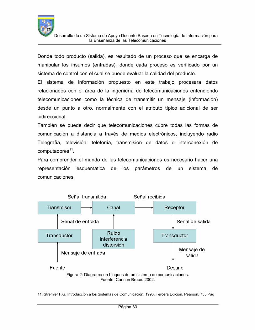
Para comprender el mundo de las telecomunicaciones es necesario hacer una
representación esquemática de los parámetros de un sistema de
comunicaciones:
Figura 2: Diagrama en bloques de un sistema de comunicaciones. Fuente: Carlson Bruce. 2002.
11. Stremler F.G, Introducción a los Sistemas de Comunicación. 1993. Tercera Edición. Pearson, 755 Pág

Desarrollo de un Sistema de Apoyo Docente Basado en Tecnología de Información para la Enseñanza de las Telecomunicaciones
Página 34
A continuación se describen cada uno de los parámetros que lo conforman:
Transductor de entrada: El mensaje puede ser producido por máquinas
o por el hombre y normalmente no es de naturaleza eléctrica. Como
ejemplos se tiene: una escena a ser transmitida por T.V., sonidos, música,
datos, parámetros físicos de un proceso tales como temperatura, presión,
humedad, señales biológicas, etc. El transductor es el encargado de
convertir cualquiera de estos mensajes en una señal eléctrica equivalente
(voltaje o corriente).
Transmisor: Adapta el mensaje ya convertido en señal eléctrica al medio
de transmisión. Esta adaptación por lo general implica un proceso de
modulación el cual consiste en alterar algún elemento de una señal fija,
llamada portadora, de acuerdo a las variaciones del mensaje. La
clasificación más general de los métodos de modulación depende del tipo
de portadora utilizada.
Medio de transmisión: Es el lazo entre el transmisor y el receptor.
Pueden ser líneas de transmisión, el aire, fibras ópticas, guías ondas, etc.
Agentes perturbadores del canal: es la atenuación que reduce el valor
de la señal y puede hacerla tan pequeña como el ruido y perderla en éste.
Distorsión que es el resultado de la respuesta imperfecta de un sistema a
la señal misma. En la práctica se diseña tratando siempre de minimizarlo.
Interferencia: Es la contaminación debida a señales externas de la misma
naturaleza que el mensaje que queremos transmitir. Ruido que es dado
gracias a que si un electrón se encuentra a una temperatura diferente al
cero absoluto tendrá una energía térmica que se manifestará con
movimientos aleatorios; y si el medio donde se encuentra el electrón es
conductor se producirá un voltaje aleatorio conocido como ruido térmico.

Desarrollo de un Sistema de Apoyo Docente Basado en Tecnología de Información para la Enseñanza de las Telecomunicaciones
Página 35
Receptor: Tiene como función rescatar la señal del medio de transmisión
y realizar las operaciones inversas del transmisor con la finalidad de
obtener el mensaje. Por lo dicho anteriormente para el modulador, la
principal labor del receptor es la demodulación. Esto implica que debe
existir un acuerdo absoluto entre transmisor y receptor, en cuanto al tipo
de funciones que cada uno debe realizar, de forma que esta operación
sea equivalente a no haber alterado el mensaje original.
Transductor de salida: Normalmente el destino de las transmisiones es
el hombre o una máquina, por lo tanto es necesario convertir la señal
eléctrica en un mensaje adecuado para ellos. Como ejemplos: Corneta,
pantalla o monitor, télex, tarjetas perforadas, graficador, la memoria de un
computador12.
El mensaje antes mencionado puede ser una señal eléctrica entendiéndose que
una señal es un símbolo, un gesto u otro tipo de signo que informa o avisa de
algo. La señal sustituye por lo tanto a la palabra escrita o al lenguaje. Las
señales obedecen a convenciones, por lo que son fácilmente
interpretadas11.También las señales pueden ser de tipo eléctrica.
Una definición de señal eléctrica puede ser el cambio de estado orientado a
eventos (p. ej. un tono, cambio de frecuencia, valor binario, alarma, mensaje,
etc.) 12. Cualquier evento que lleve implícita cierta información.
Existe un tipo de comunicación conocida como banda base que se define como
la transmisión de señal sin modulación el nombre proviene del hecho que una
señal en banda base no incluye la traslación en frecuencia del espectro del
mensaje que caracteriza una modulacion11.
11. Stremler F.G, Introducción a los Sistemas de Comunicación. 1993. Tercera Edición. Pearson, 755 Pág 12. Carlson Bruce, Communication System. 2002. Cuarta Edicion. McGraw-Hill, 793 Pág

Desarrollo de un Sistema de Apoyo Docente Basado en Tecnología de Información para la Enseñanza de las Telecomunicaciones
Página 36
El mensaje que se desea transmitir debe sufrir un proceso de adaptación
conocido como Modulación que consiste en la alteración sistemática de una
forma de onda conocida como portadora en función de las características de otra
forma de onda11.
La modulación también es conocida como el proceso que realizan los módems
para adaptar la información digital a las características de las líneas telefónicas
analógicas12.
Figura 3: traslación del mensaje a través de la modulación. Fuente: propia
2.4 Tipos de modulación analógica Muchas señales de entrada no pueden ser enviadas directamente hacia el canal,
como vienen del transductor. Para eso se modifica una onda portadora, cuyas
propiedades se adaptan mejor al medio de comunicación en cuestión, para
representar el mensaje. A continuación se describirán los tipos de modulación
analógica:
11. Stremler F.G, Introducción a los Sistemas de Comunicación. 1993. Tercera Edición. Pearson, 755 Pág 12. Carlson Bruce, Communication System. 2002. Cuarta Edicion. McGraw-Hill, 793 Pág
Desarrollo de un Sistema de Apoyo Docente Basado en Tecnología de Información para la Enseñanza de las Telecomunicaciones
Página 37
Modulación por amplitud (AM): es una modulación lineal que consiste en
modular la amplitud de la onda portadora de forma que su valor cambie de
acuerdo con las variaciones de la señal moduladora, que es la información que
se va a transmitir. La modulación de amplitud es equivalente a la modulación en
doble banda lateral con reinserción de portadora13.
El mensaje o la información a transmitir deben cumplir con ciertas condiciones
de acondicionamiento entre las cuales se tienen:
El mensaje x(t) estará limitado en banda.
El mensaje x(t) estará normalizado, esto es, |x(t)| <= 1. En este caso la
potencia.
El promedio de x(t) será también menor e igual que 1 si proviene de una
fuente ergódica.
Muchas veces se supondrá que el mensaje es un tono x(t)=AmCosωmt lo
cual tiene sentido dado que el análisis de Fourier permite representar
señales en función de sinusoides y así aplicar superposición si los
sistemas son lineales. Por otra parte como la modulación de onda
continua utiliza portadora sinusoidal, la señal resultante (si el ancho de
banda fraccional es pequeño) puede analizarse como una sinusoide pura.
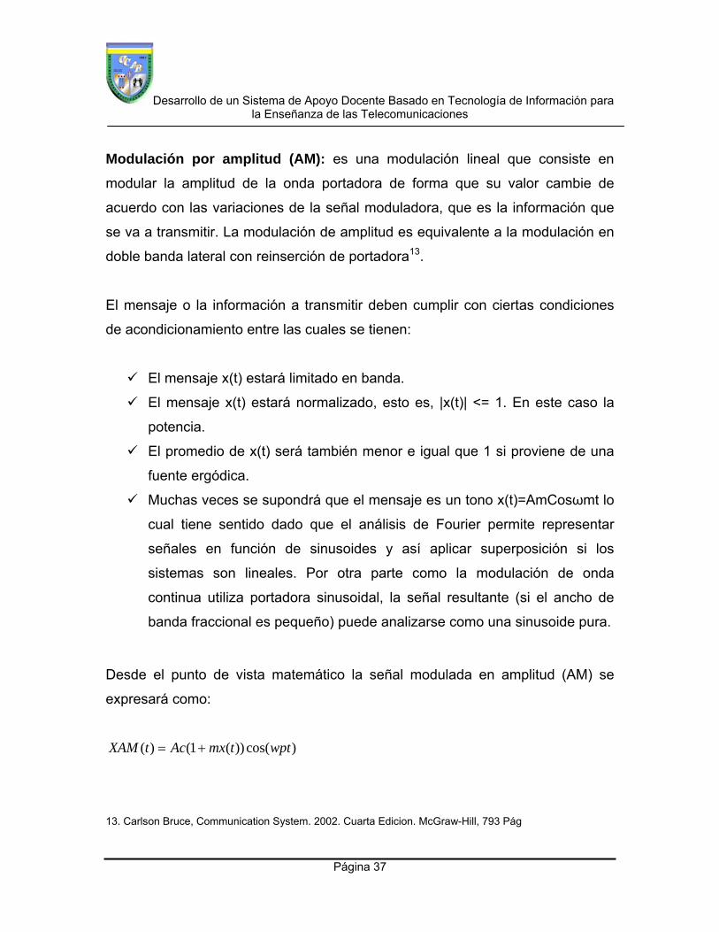
Desde el punto de vista matemático la señal modulada en amplitud (AM) se
expresará como:
)cos())(1()( wpttmxActXAM
13. Carlson Bruce, Communication System. 2002. Cuarta Edicion. McGraw-Hill, 793 Pág

Desarrollo de un Sistema de Apoyo Docente Basado en Tecnología de Información para la Enseñanza de las Telecomunicaciones
Página 38
Donde m es el índice de modulación que se encuentra entre 0 y 1. También se
puede calcular índice de modulación estableciendo una relación de amplitud del
mensaje/ amplitud de la portadora para señal de tono simple.
Gráficamente:
0 50 100 150 200 250-2
-1
0
1
2señal original
tiempo
ampl
itud
-4000 -3000 -2000 -1000 0 1000 2000 3000 40000
0.2
0.4
0.6
0.8
Espectro en frecuencia
ampl
itud
Grafica 1: Representación en forma de onda de la señal mensaje. Fuente: propia.

Desarrollo de un Sistema de Apoyo Docente Basado en Tecnología de Información para la Enseñanza de las Telecomunicaciones
Página 39
0 50 100 150 200 250-2
-1
0
1
2portadora
tiem po
ampl
itud
-4000 -3000 -2000 -1000 0 1000 2000 3000 40000
0.2
0.4
0.6
0.8
E s pec tro en frec uenc ia
ampl
itud
Grafica 2: Representación en forma de onda de la señal portadora. Fuente: propia.
0 50 100 150 200 250 300 350 400 450 500-2
-1
0
1
2señal modulada con m=0.5
tiempo
ampl
itud
-4000 -3000 -2000 -1000 0 1000 2000 3000 40000
0.2
0.4
0.6
0.8
Espectro de frecuenc ia
ampl
itud
Grafica 3: Representación en forma de onda de la señal modulada en amplitud. Fuente: propia.
Desarrollo de un Sistema de Apoyo Docente Basado en Tecnología de Información para la Enseñanza de las Telecomunicaciones
Página 40
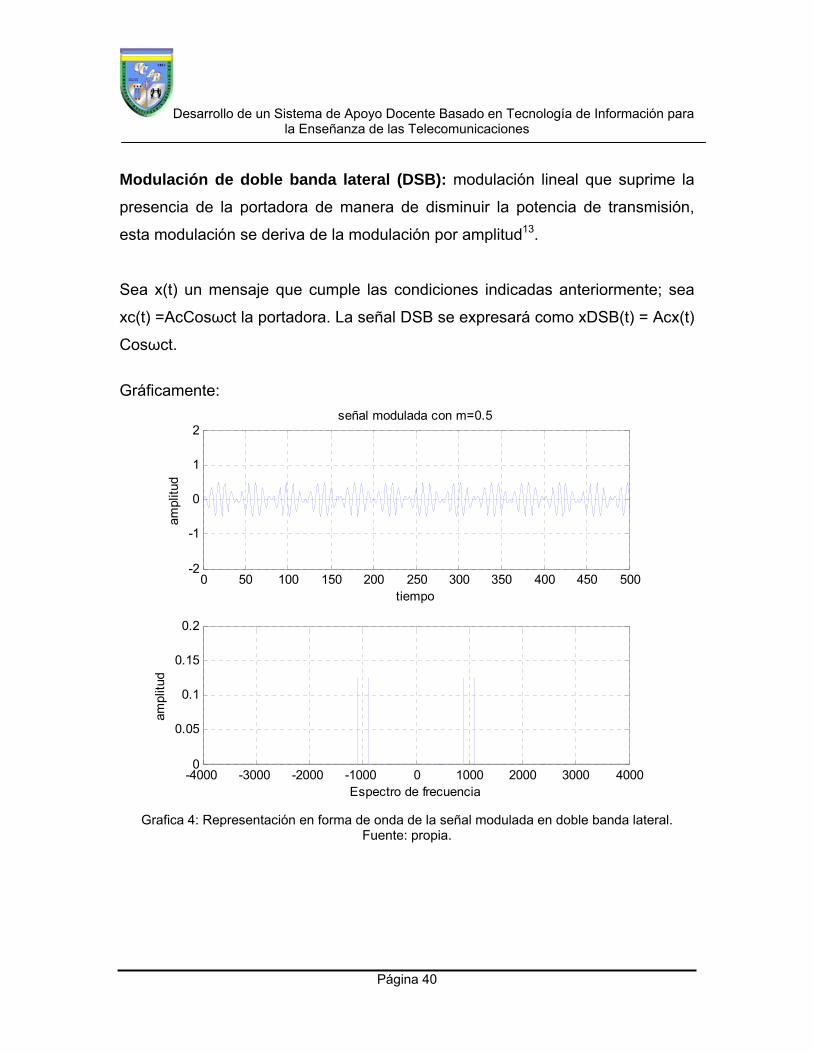
Modulación de doble banda lateral (DSB): modulación lineal que suprime la
presencia de la portadora de manera de disminuir la potencia de transmisión,
esta modulación se deriva de la modulación por amplitud13.
Sea x(t) un mensaje que cumple las condiciones indicadas anteriormente; sea
xc(t) =AcCosωct la portadora. La señal DSB se expresará como xDSB(t) = Acx(t)
Cosωct.
Gráficamente:
0 50 100 150 200 250 300 350 400 450 500-2
-1
0
1
2señal modulada con m=0.5
tiempo
ampl
itud
-4000 -3000 -2000 -1000 0 1000 2000 3000 40000
0.05
0.1
0.15
0.2
Espectro de frecuencia
ampl
itud
Grafica 4: Representación en forma de onda de la señal modulada en doble banda lateral. Fuente: propia.

Desarrollo de un Sistema de Apoyo Docente Basado en Tecnología de Información para la Enseñanza de las Telecomunicaciones
Página 41
Modulación de banda lateral única (SSB): modulación lineal que suprime la
presencia de la portadora y de una banda lateral de manera de disminuir la
potencia de transmisión, esta modulación se deriva de la modulación de doble
banda lateral13.
Supongamos que la expresión de la señal SSB es la siguiente:
)()(')cos()(2
1)( wptsentxwpttxACtXSSB
Donde x(t) está limitada en banda. Gráficamente se tiene:
0 50 100 150 200 250-2
-1
0
1
2modulacion ssb banda lateral inferior
tiempo
ampl
itud
-4000 -3000 -2000 -1000 0 1000 2000 3000 40000
0.1
0.2
0.3
0.4
Espectro de frecuencia
ampl
itud
Grafica 5: Representación en forma de onda de la señal modulada en banda lateral única. Fuente: propia.
13. Carlson Bruce, Communication System. 2002. Cuarta Edicion. McGraw-Hill, 793 Pág

Desarrollo de un Sistema de Apoyo Docente Basado en Tecnología de Información para la Enseñanza de las Telecomunicaciones
Página 42
0 50 100 150 200 250-2
-1
0
1
2modulacion ssb banda lateral superior
tiempo
ampl
itud
-4000 -3000 -2000 -1000 0 1000 2000 3000 40000
0.1
0.2
0.3
0.4
Espectro de frecuencia
ampl
itud
Grafica 6: Representación en forma de onda de la señal modulada en banda lateral única. Fuente:propia
2.5 Tipos de modulación digital También existe un equivalente digital de modulación que significa que la
información que se requiere transmitir esta en un formato digital por lo cual solo
tiene dos valores posibles de “0” lógico y “1” que representan niveles de voltaje
(“1”= 5V y “0”= 0V), este tipo de señal también es conocida como una banda
base digital ya que ella es la que va a ser modulada.
Existen dos formas de generar mensajes digitales:
1. Que la señal sea de naturaleza discreta y solo necesite acondicionarse
para su transmisión.

Desarrollo de un Sistema de Apoyo Docente Basado en Tecnología de Información para la Enseñanza de las Telecomunicaciones
Página 43
2. O que la señal sea de naturaleza analógica y necesite de procesos
previos de conversión analógica/digital para luego de ser acondicionada
para transmitirla.
Esta conversión analógica digital se conoce como modulación PCM modulación
por codificación de pulsos.
Para llevar a cabo esta modulación se deben realizar los siguientes pasos:
Muestreo y retención de la señal analógica.
Cuantificación de la señal muestreada.
Codificación de la señal cuantificada.
Muestreo y retención
Esta actividad consta de tomar el valor de una señal a intervalos de tiempo
regulares. El intervalo de tiempo entre cada 2 instantes de muestreo
consecutivos es igual a “TS” segundos y se le denomina PERIODO DE
MUESTREO (TS)14.
Figura 4: Representación en forma de onda de la señal muestreada.
Fuente:propia
14 Stremler F.G, Introducción a los Sistemas de Comunicación. 1993. Tercera Edición. Pearson, 755 Pág.

Desarrollo de un Sistema de Apoyo Docente Basado en Tecnología de Información para la Enseñanza de las Telecomunicaciones
Página 44
En su análisis se lo puede clasificar en tres tipos:
Ideal: El instante de muestreo (T), tiende a cero, es decir se trata de una
sucesión de muestras infinitas.
Natural: El tren de pulsos posee un período T de cualquier valor distinto de cero.
LA función muestreada tendrá un número infinito de valores en el período de
muestreo.
Con retención: (Sample and Hold) Es el que se emplea en la práctica, y
consiste en tomar la muestra y retener el valor un cierto tiempo hasta que
comience el próximo período de muestreo.
Figura 5: Señal muestreada de forma natural. Fuente: propia.
Figura 6: Representación de una señal muestreada y retenida.
Fuente: propia

Desarrollo de un Sistema de Apoyo Docente Basado en Tecnología de Información para la Enseñanza de las Telecomunicaciones
Página 45
Cuantificación Proceso que consiste en transformar los niveles de amplitud continuos de la
señal de entrada previamente muestreada, en un conjunto de niveles discretos
previamente establecidos14.
Figura 7: Representación de la cuantificación de una señal. Fuente: propia
Codificación Proceso que consiste en convertir los pulsos cuantificados en un grupo
equivalente de pulsos binarios de amplitud constante. En la práctica para la
transmisión de voz digitalizada se emplean sistemas de ocho bit por muestra, lo
que equivale a trabajar con 256 niveles de cuantificación14.
Figura 8: Representación de la codificación de una señal.
Fuente: propia.
14 Stremler F.G, Introducción a los Sistemas de Comunicación. 1993. Tercera Edición. Pearson, 755 Pág.
Desarrollo de un Sistema de Apoyo Docente Basado en Tecnología de Información para la Enseñanza de las Telecomunicaciones
Página 46
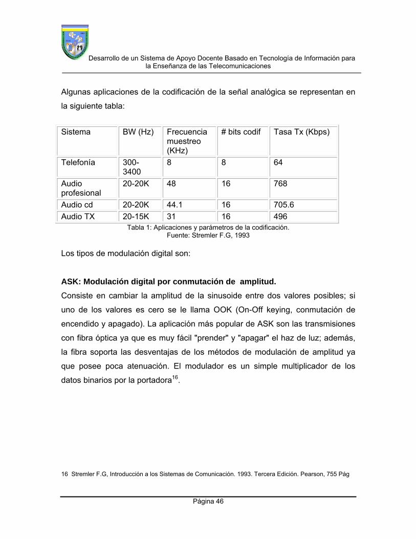
Algunas aplicaciones de la codificación de la señal analógica se representan en
la siguiente tabla:
Sistema BW (Hz) Frecuencia muestreo (KHz)
# bits codif Tasa Tx (Kbps)
Telefonía 300-3400
8 8 64
Audio profesional
20-20K 48 16 768
Audio cd 20-20K 44.1 16 705.6
Audio TX 20-15K 31 16 496 Tabla 1: Aplicaciones y parámetros de la codificación.
Fuente: Stremler F.G, 1993 Los tipos de modulación digital son:
ASK: Modulación digital por conmutación de amplitud.
Consiste en cambiar la amplitud de la sinusoide entre dos valores posibles; si
uno de los valores es cero se le llama OOK (On-Off keying, conmutación de
encendido y apagado). La aplicación más popular de ASK son las transmisiones
con fibra óptica ya que es muy fácil "prender" y "apagar" el haz de luz; además,
la fibra soporta las desventajas de los métodos de modulación de amplitud ya
que posee poca atenuación. El modulador es un simple multiplicador de los
datos binarios por la portadora16.
16 Stremler F.G, Introducción a los Sistemas de Comunicación. 1993. Tercera Edición. Pearson, 755 Pág

Desarrollo de un Sistema de Apoyo Docente Basado en Tecnología de Información para la Enseñanza de las Telecomunicaciones
Página 47
0 0 . 0 5 0 . 1 0 . 1 5 0 . 2 0 . 2 5 0 . 3 0 . 3 5 0 . 4 0 . 4 5 0 . 5-1
0
1
2
t ie m p o
ampl
itud
s e ñ a l re c o d ific a d a u n ip o la r N R Z
2 3 5 0 2 4 0 0 2 4 5 0 2 5 0 0 2 5 5 0 2 6 0 0 2 6 5 0 2 7 0 0 2 7 5 0-1 . 5
-1
-0 . 5
0
0 . 5
1
s e ñ a l m o d u la d a A S K
t ie m p o
ampl
itud
-4 0 0 0 -3 0 0 0 -2 0 0 0 -1 0 0 0 0 1 0 0 0 2 0 0 0 3 0 0 0 4 0 0 00
1
2
3
4x 1 0
7 e s p e c t ro d e A S K
fre c u e n c ia
ampl
itud
Grafica 7: Representación en forma de onda de la señal modulada por conmutación de amplitud. Fuente: propia.
FSK: Modulación digital por cambios de frecuencia. Consiste en variar la frecuencia de la portadora de acuerdo a los datos. Si la
fase de la señal FSK es continua, es decir entre un bit y el siguiente la fase de la
sinusoide no presenta discontinuidades, a la modulación se le da el nombre de
CPFSK (Continuous Phase FSK, modulación por conmutación de frecuencias de
fase continua)15.
15 Carlson Bruce, Communication System. 2002. Cuarta Edición. McGraw-Hill, 793 Pág.

Desarrollo de un Sistema de Apoyo Docente Basado en Tecnología de Información para la Enseñanza de las Telecomunicaciones
Página 48
0 0.05 0.1 0.15 0.2 0.25 0.3 0.35 0.4 0.45 0.5-1
0
1
2
tiempo
ampl
itud
señal recodificada unipolar NRZ
1400 1420 1440 1460 1480 1500 1520 1540 1560 1580 1600
-1
0
1
señal modulada en FSK
tiempo
ampl
itud
-4000 -3000 -2000 -1000 0 1000 2000 3000 40000
5
10
15
x 106 espectro de FSK
frecuencia
ampl
itud
Grafica 8: Representación en forma de onda de la señal modulada por conmutación de de
frecuencia. Fuente: propia.
.
PSK: Modulación digital por cambio de fase. Aunque PSK no es usado directamente, es la base para entender otros sistemas
de modulación de fase multinivel. Consiste en variar la fase de la sinusoide de
acuerdo a los datos. Para el caso binario, las fases que se seleccionan son 0 y
180. En este caso la modulación de fase recibe el nombre de PRK (Phase
Reversal Keying, modulación por conmutación de fase)16.
16 Stremler F.G, Introducción a los Sistemas de Comunicación. 1993. Tercera Edición. Pearson, 755 Pág

Desarrollo de un Sistema de Apoyo Docente Basado en Tecnología de Información para la Enseñanza de las Telecomunicaciones
Página 49
0 0.05 0.1 0.15 0.2 0.25 0.3 0.35 0.4 0.45 0.5-1
0
1
2
tiempo
ampl
itud
señal recodificada unipolar NRZ
900 950 1000 1050 1100 1150
-1
0
1
señal modulada PSK
tiempo
ampl
itud
-4000 -3000 -2000 -1000 0 1000 2000 3000 40000
5
10
15x 10
6 espectro de PSK
frecuencia
ampl
itud
Grafica 9: Representación en forma de onda de la señal modulada por conmutación de de fase. Fuente: propia.
2.6 Técnicas Didácticas Desde tiempos remotos han existido enfoques alternativos sobre el origen y la
adquisición del conocimiento: el Empirismo y el Racionalismo.
El Racionalismo ve al conocimiento como derivado de la razón sin la ayuda de
los sentidos. Se usa la razón para descubrir esos conocimientos innatos que
están dentro de la mente. Aprender es recordar y descubrir lo que está dentro
de nosotros. Desde esta perspectiva los aspectos críticos del diseño de
instrucción se centran en como estructurar mejor la nueva información para
facilitar su adquisición y evocación.

Desarrollo de un Sistema de Apoyo Docente Basado en Tecnología de Información para la Enseñanza de las Telecomunicaciones
Página 50
El Empirismo ve a la experiencia como la fuente del conocimiento, se nace sin
conocimiento y todo se aprende a través de interacciones con el ambiente. En el
conductismo (con estas raíces filosóficas) tiene sus raíces el diseño de
instrucción. Desde esta perspectiva, los aspectos críticos del diseño de
instrucción se centran en como manipular el ambiente para mejorar y garantizar
que ocurran las asociaciones apropiadas.
2.7 Tipos de aprendizaje explicados por los diferentes enfoques El Conductismo prescribe estrategias útiles para construir y reforzar
asociaciones estímulo-respuesta, incluyendo el uso de indicios, práctica y
refuerzo, luego es efectivo para explicar aprendizajes que tiene que ver con
discriminación, generalización, asociaciones, y desempeño automático de un
procedimiento. Hace énfasis en el diseño del ambiente para lograr la
transferencia del conocimiento al aprendiz. No puede explicar aprendizajes de
alto nivel o de mucha profundidad de procesamiento como por ejemplo la
resolución de problemas.
Según los cognitivistas el aprendizaje es un cambio discreto entre los estados
del conocimiento. Se ocupan de cómo la información es recibida, organizada,
almacenada y recuperada. Da mucha importancia a los conocimientos previos y
a cómo se adquiere el conocimiento. El estudiante es activo en el proceso de
aprendizaje
El Cognocitivismo es apropiado para explicar aprendizajes complejos como
razonamiento, resolución de problemas, procesamiento de información,
haciendo énfasis en las estrategias de procesamiento para lograr en forma
eficiente la transferencia de conocimiento a los aprendices.

Desarrollo de un Sistema de Apoyo Docente Basado en Tecnología de Información para la Enseñanza de las Telecomunicaciones
Página 51
Para los Constructivistas el aprendizaje es la creación de significados a partir
de experiencias. Creen que la mente filtra lo que nos llega del mundo para
producir una propia y única realidad Consideran a la mente como fuente de todo
significado. Todo conocimiento nuevo parte de uno previo. El estudiante es
activo y participante en la elaboración e interpretación de los contenidos de
aprendizaje.
El Constructivismo es apropiado para explicar aprendizajes complejos y poco
estructurados. Es efectivo en las etapas de adquisición de conocimiento
avanzado donde los prejuicios y malas interpretaciones adquiridas durante la
etapa inicial pueden ser descubiertos, modificados o eliminados17
17 Ertmer, P y Newby T. (1993). Conductismo, cognitivismo y constructivismo: una comparación de los aspectos críticos desde la perspectiva del diseño de instrucción. Traducción de Ferstadt, N. y Mario Szcaurek, M. Universidad Pedagógica Experimental Libertador. Instituto Pedagógico de Caracas.

Desarrollo de un Sistema de Apoyo Docente Basado en Tecnología de Información para la Enseñanza de las Telecomunicaciones
Página 52
2.8 Simulación Didáctica Desde el punto de vista conceptual, una simulación se define ordinariamente
como “la puesta en marcha, o la ejecución, de un modelo” En consecuencia, una
simulación científica se define como la puesta en funcionamiento de un modelo
científico18. La siguiente figura muestra el diagrama de flujo de un análisis de
simulaciones didácticas:
Figura 9: Análisis de simulaciones didácticas Fuente: GUTIERREZ, R. y PINTÓ, R., (2004)
2.9 Ambientes Colaborativos de Aprendizaje
El aprendizaje en ambientes colaborativos y cooperativos busca propiciar
espacios en los cuales se dé el desarrollo de habilidades individuales y grupales
a partir de la discusión entre los estudiantes al momento de explorar nuevos
conceptos, siendo cada quien responsable tanto de su propio aprendizaje como
del de los demás miembros del grupo. Se busca que estos ambientes sean ricos
en posibilidades y, más que organizadores de la información, propicien el
crecimiento del grupo18.
18. GUTIERREZ, R. y PINTÓ, R., (2004) Models and Simulations. Construction of a Theoretically Grounded Analytic
Instrument. En: E. Mechlová (ed), Proceedings of the GIREP 2004 International Conference Teaching and Learning
Physics in New Contexts. Selected Papers. Ostrava, Czech Republic: University of Ostrava, p. 157-158.

Desarrollo de un Sistema de Apoyo Docente Basado en Tecnología de Información para la Enseñanza de las Telecomunicaciones
Página 53
El desarrollo de una herramienta de software que apoye los ambientes
colaborativos de aprendizaje, requiere revisión de estos conceptos e
identificación de los elementos que componen un contexto educativo para este
tipo de aprendizaje. A continuación, se presenta una breve síntesis conceptual y
se describen sus características funcionales, como base para integrar estas
características en un software que sirva de herramienta para estos procesos.
Diferentes teorías del aprendizaje encuentran aplicación en los ambientes
colaborativos; entre éstas, los enfoques de Piaget y de Vygotsky basados en la
interacción social. Para estos autores, la mediación social entre el niño y su
entorno cultural son elementos básicos en su desarrollo.
Una recopilación de estudios sobre aprendizaje colaborativo [3] permite
compartir la siguiente definición, adecuada de Johnson, D. y Jonson; Conjunto
de métodos de instrucción o entrenamiento para uso en grupos pequeños, así
como de estrategias para propiciar el desarrollo de habilidades mixtas
(aprendizaje y desarrollo personal y social), donde cada miembro de grupo es
responsable tanto de su aprendizaje como del de los restantes miembros del
grupo.
2.10 Elementos básicos para propiciar el aprendizaje colaborativo Los cuatro elementos básicos que deben estar presentes para que pequeños
grupos realmente vivan experiencias de aprendizaje en ambientes colaborativos
son:
2.11 Interdependencia positiva Este es el elemento central, abarca las condiciones organizacionales y de
funcionamiento que deben darse al interior del grupo. Sus miembros deben
necesitarse los unos a los otros y confiar en el entendimiento y éxito de cada
persona. Considera aspectos de interdependencia en el establecimiento de
metas, tareas, recursos, roles, premios.

Desarrollo de un Sistema de Apoyo Docente Basado en Tecnología de Información para la Enseñanza de las Telecomunicaciones
Página 54
2.12 Contribución individual Cada miembro del grupo debe asumir íntegramente su tarea y, además, tener
los espacios para compartirla con el grupo y recibir sus contribuciones.
2.13 Habilidades personales y de grupo La vivencia del grupo debe permitir a cada miembro de éste el desarrollo y
potencialización de sus habilidades personales. De igual forma permitir el
crecimiento del grupo y la obtención de habilidades grupales como: escucha,
participación, liderazgo, coordinación de actividades, seguimiento y evaluación.
2.14 Ambientes colaborativos soportados con tecnología informática Lo innovador en los ambientes colaborativos soportados con tecnología es la
introducción de la informática a estos espacios, sirviendo las redes virtuales de
soporte, lo que da origen a los ambientes CSCL (Computer Supported
Collaborative Learning - Aprendizaje colaborativo asistido por computador).
La introducción de la informática a los ambientes colaborativos, abre nuevas
posibilidades entre las cuales se resaltan la posibilidad de:
Romper las barreras geográficas. La utilización de la tecnología como
medio de comunicación (sincrónica/asincrónica), permite a un grupo no
necesariamente localizado en el mismo espacio físico, la interacción e
intercambio.
Que el grupo se encuentre en nuevos espacios, diferentes a los
cotidianos, los cuales tienen un significado de mágicos y atrayentes.
Desarrollo de un Sistema de Apoyo Docente Basado en Tecnología de Información para la Enseñanza de las Telecomunicaciones
Página 55
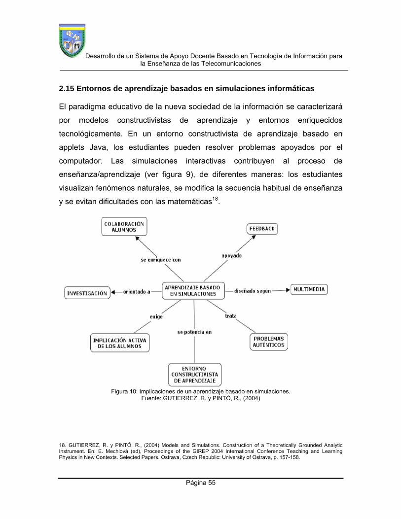
2.15 Entornos de aprendizaje basados en simulaciones informáticas El paradigma educativo de la nueva sociedad de la información se caracterizará
por modelos constructivistas de aprendizaje y entornos enriquecidos
tecnológicamente. En un entorno constructivista de aprendizaje basado en
applets Java, los estudiantes pueden resolver problemas apoyados por el
computador. Las simulaciones interactivas contribuyen al proceso de
enseñanza/aprendizaje (ver figura 9), de diferentes maneras: los estudiantes
visualizan fenómenos naturales, se modifica la secuencia habitual de enseñanza
y se evitan dificultades con las matemáticas18.
Figura 10: Implicaciones de un aprendizaje basado en simulaciones. Fuente: GUTIERREZ, R. y PINTÓ, R., (2004)
18. GUTIERREZ, R. y PINTÓ, R., (2004) Models and Simulations. Construction of a Theoretically Grounded Analytic Instrument. En: E. Mechlová (ed), Proceedings of the GIREP 2004 International Conference Teaching and Learning Physics in New Contexts. Selected Papers. Ostrava, Czech Republic: University of Ostrava, p. 157-158.

Desarrollo de un Sistema de Apoyo Docente Basado en Tecnología de Información para la Enseñanza de las Telecomunicaciones
Página 56
A continuación se presentara un ejemplo gráfico de simulación didáctica:
Figura 11: Receptor de radio AM. Fuente: propia
2.16 Lenguaje de programación con orientación a la ciencia y tecnología Matlab MATLAB es uno de los simuladores más útiles que existen para poner a punto
métodos numéricos en distintas materias de ingeniería. Por ser una herramienta
de alto nivel, el desarrollo de programas numéricos con MATLAB puede requerir
menos de esfuerzo que en lenguajes de programación convencionales, como
Fortran, Pascal, C/C++,Java o Visual Basic.

Desarrollo de un Sistema de Apoyo Docente Basado en Tecnología de Información para la Enseñanza de las Telecomunicaciones
Página 57
MATLAB es el nombre abreviado de “MATrix LABoratory” MATLAB es un
programa para realizar cálculos numéricos con vectores y matrices. Como caso
particular, puede también trabajar con números escalares tanto reales como
complejos, con cadenas de caracteres y con otras estructuras de información
más complejas. Una de las capacidades más atractivas es la de realizar una
amplia variedad de gráficas en dos y tres dimensiones. MATLAB tiene también
un lenguaje de programación propio.
MATLAB es un gran programa de cálculo técnico y científico. Para ciertas
operaciones es muy rápido, cuando puede ejecutar sus funciones en código
nativo con los tamaños más adecuados para aprovechar sus capacidades de
vectorización. En otras aplicaciones resulta bastante más lento que el código
equivalente desarrollado en C/C++ o Fortran. En la versión 6.5 MATLAB han
incorporado un acelerador JIT (Just In Time), que mejora significativamente la
velocidad de ejecución de los archivos *.m en ciertas circunstancias, por ejemplo
cuando no se hacen llamadas a otros archivos *.m no se utilizan estructuras y
clases, etc. Aunque limitado por el momento, cuando se aplica mejora
sensiblemente la velocidad, haciendo innecesarias ciertas técnicas utilizadas en
versiones anteriores como la vectorización de los algoritmos. En cualquier caso,
el lenguaje de programación de MATLAB siempre es una magnífica herramienta
de alto nivel para desarrollar aplicaciones técnicas, fácil de utilizar y que, como
ya se ha dicho, aumenta significativamente la productividad de los
programadores respecto a otros entornos de desarrollo.
MATLAB dispone de un código básico y de varias librerías especializadas
(toolboxes). En estos apuntes se hará referencia exclusiva al código básico.

Desarrollo de un Sistema de Apoyo Docente Basado en Tecnología de Información para la Enseñanza de las Telecomunicaciones
Página 58
Figura 12: Pantalla principal del software MATLAB. Fuente: propia
Los ejemplos gráficos fueron mostrados en la sección donde se explicaron los
tipos de modulación analógica y digital. Las palabras reservadas utilizadas por el
lenguaje serán mostradas en la figura:

Desarrollo de un Sistema de Apoyo Docente Basado en Tecnología de Información para la Enseñanza de las Telecomunicaciones
Página 59
Figura 13: Código fuente del software MATLAB. Fuente: propia.

Desarrollo de un Sistema de Apoyo Docente Basado en Tecnología de Información para la Enseñanza de las Telecomunicaciones
Página 60
CAPITULO III
3. MARCO METODOLOGICO
3.1 Características metodológicas del levantamiento de información.
Para esta etapa de levantamiento de información, se obtuvo información
acerca de los contenidos de las materias seleccionadas para el desarrollo de la
herramienta y las estrategias didácticas empleadas por los docentes para
impartir dichos contenidos, los mismos fueron determinados según su nivel de
dificultad en el proceso de enseñanza. Por otro lado también se recopiló
información acerca de las características de programación del software
MATLAB. Para ello se realizó una investigación de campo y de tipo documental.
La investigación de campo se efectuó a través de observación y encuestas
(entrevistas).
La investigación documental se realiza por medio de documentos (libros,
programas de las materias que conforman el pemsum de Ing. De
telecomunicaciones, guías de trabajo, material recopilado en línea, etc.).
Estrategia de Campo: Esta estrategia permitió por medio de entrevistas
seleccionar los tópicos contenidos en las materias señales y sistemas I,
comunicaciones I y comunicaciones II que serán desarrollados, procesados y
presentados en el Sistema de información académico.
Cabe destacar que esta estrategia también permitió definir los datos a manejar,
los procesos a ejecutar y la presentación de los resultados obtenidos.
Es importante destacar que el proceso de selección de los tópicos de las
materias antes mencionadas, fue realizado tomando en cuenta su nivel de
complejidad matemática, abstracción y nivel de dificultad en la estrategia
didáctica de enseñanza utilizada.

Desarrollo de un Sistema de Apoyo Docente Basado en Tecnología de Información para la Enseñanza de las Telecomunicaciones
Página 61
Estrategia Documental: Consistió en el levantamiento de información contenida
en documentos en línea, programas de asignaturas, guías de trabajo, textos
orientados al área de comunicaciones y libros de metodología. Básicamente esta
etapa estuvo orientada la delimitación de los temas que se desarrollaran en la
herramienta, estrategias didácticas de enseñanza y los Sistemas de Información
Basados en Simuladores Programables.
En relación a la relimitación de los temas desarrollados en la herramienta SAET,
esta información fue obtenida a través de la estrategia de campo utilizada.
Luego se levantó información sobre estrategias didácticas de enseñanza, así
como los tipos de aprendizaje explicados por diferentes enfoques (Conductismo,
Cognocitivismo y Constructivismo).
Finalmente con respecto a los Sistemas de Información basados en simuladores
programables (MATLAB), se levanto información sobre el procesamiento
matemático de los datos, la presentación de la información y los elementos de
programación necesarios para el desarrollo de la herramienta.
3.2 Problema
La formación del Ingeniero en Telecomunicaciones se fundamenta en las
siguientes áreas:
Formación Básica y Gerencial, en la cual se incluyen las asignaturas
relativas a la formación científico-humanista y gerencial, requeridas para
cualquier profesional de la ingeniería, especialmente basadas en el
modelo de las actuales carreras de ingeniería de la UCAB.
Tecnología de las Comunicaciones, en la cual se incluyen todas las
asignaturas requeridas para formar al estudiante en todos los aspectos
relativos a las tecnologías de las comunicaciones, en todas sus
especialidades.

Desarrollo de un Sistema de Apoyo Docente Basado en Tecnología de Información para la Enseñanza de las Telecomunicaciones
Página 62
Electrónica, en donde se incluyen los elementos fundamentales que en
materia de electrónica deben conocer los ingenieros en
telecomunicaciones, para ser capaces de gerenciar proyectos
especializados desde sus etapas de análisis y diseño hasta la gestión y
evaluación de los mismos.
Informática, la cual contempla todos los aspectos necesarios en materia
de informática, para formar ingenieros capaces de comprender y aplicar
tecnologías de información.
Telemática, la cual abarca los elementos de formación requeridos para
conocer y poner en práctica soluciones que se caractericen por la fuerte
relación entre las tecnologías de las comunicaciones y la informática.
Sistemas de comunicaciones analógicas y digitales, la cual contempla
todo lo referentes a comunicaciones analógicas, comunicaciones
digitales, microondas, antenas y propagación de ondas y
radiocomunicaciones.
Para apoyar el desarrollo de la carrera en las diferentes áreas que la conforman,
se necesita instalar una plataforma tecnológica para el procesamiento inteligente
en el soporte de toma de decisiones y desarrollo de servicios con un alto valor
agregado de tecnología, ajustada a las necesidades de una sociedad que
requiere de servicios de alta tecnología para la educación, el entrenamiento, el
trabajo cooperativo, análisis y filtrado de informaciones fundamentadas en una
visión moderna de aplicación y creación tecnológica.
La carrera de Ingeniería de Telecomunicaciones necesita de sistemas de
información que apoyen el proceso enseñanza-aprendizaje, que a su vez cumpla
con los requerimientos de entrenamiento para formación de profesionales con
elevadas capacidades de evaluación y aplicación de tecnologías, englobados en
una visión de desarrollo de conocimientos en el área de las Telecomunicaciones.

Desarrollo de un Sistema de Apoyo Docente Basado en Tecnología de Información para la Enseñanza de las Telecomunicaciones
Página 63
3.3 Tipo de investigación
El tipo de investigación a desarrollar en esta propuesta es un proyecto factible ya
que se pretende desarrollar un sistema de apoyo docente en la enseñanza de
las telecomunicaciones, este sistema implica cambios en una realidad dada de
tipo educativa. Además que según la naturaleza factible de esta propuesta para
el diseno del sistema serán empleados un conjunto de métodos y técnicas
(dentro de la perspectiva de sistemas de información), que deberán cumplir con
ciertos requisitos que le proporcionaran validez científica al sistema propuesto19.
3.4 Diseño del trabajo especial de grado
Para establecer las estrategias que enmarcaran el proceso de enseñanza-
aprendizaje en el campo de las telecomunicaciones se realizaran entrevistas con
personal docente que imparte las materias relacionadas con el campo de estudio
(señales y sistemas I y II y comunicaciones I y II) “La entrevista es un contacto
interpersonal a nivel de conversación, con el objetivo de obtener información en
relación con el problema de investigación planteado. Entre sus características se
encuentran, si no es conducida, el entrevistado expresa libremente sus
opiniones, si es conducida se atiende a una estructura o procedimiento20. La
finalidad de estas entrevistas es indagar sobre las estrategias (didácticas)
utilizadas por los docentes de las materias antes mencionadas y preguntarles
cuales temas de sus materias son mas difíciles de explicar (por el alto contenido
matemático y de abstracción), de manera de desarrollar la herramienta de esta
propuesta en base a esos temas, lo que desde el punto de vista de proyecto se
le llamaría el levantamiento de información.
19. Balestrini Mirian. Como se elabora un proyecto de investigación. Sexta edición. Consultores y asociados 20. Rosas, Mirna(2002). Guía Práctica de Investigación. Editorial Trillas

Desarrollo de un Sistema de Apoyo Docente Basado en Tecnología de Información para la Enseñanza de las Telecomunicaciones
Página 64
Una vez efectuado el levantamiento de información con los profesores se
recopilaran los contenidos relevantes en el campo de telecomunicaciones para el
proceso enseñanza aprendizaje dentro de las materias señaladas y se utilizara
una metodología ACOSIAN (Análisis y Concepción de Sistemas de Información
Automatizados Normalizados), para el análisis y diseno del sistema, propuesta
por Profesor de la asignatura de Análisis y Diseño de Sistemas en el postgrado
de Sistemas de Información de la UCAB, Jesús Ramírez, según su guía no
publicada. Esta metodología permitirá desarrollar el sistema de información para
el procesamiento de los contenidos seleccionados.
3.5 Instrumentos
Después de realizar el levantamiento de la información se utilizara un software
para el procesamiento de los datos con el fin de representar los resultados de la
simulación de manera sencilla y comprensible y que a su vez permita la
interacción de forma amigable y didáctica con el usuario. El software a utilizar es
el matlab versión 7.2 anteriormente descrito funcional y técnicamente en el
marco teorico21.
3.6 Procedimientos
Estos serán los pasos a seguir para el desarrollo del sistema SAET:
1. Recopilación de información relevante donde se destacaran los temas
que tengan alto grado de dificultad para el proceso enseñanza-
aprendizaje (por su estructura matemática y dificultad para una
implementación técnica). Esta recopilación se hará en base a entrevistas
con profesores de las materias señales y sistemas I y II y comunicaciones
I y II.
21. Del Rosario, Zuleima. Guía para la elaboración de reportes de investigación. UCAB 2006
Desarrollo de un Sistema de Apoyo Docente Basado en Tecnología de Información para la Enseñanza de las Telecomunicaciones
Página 65
2. En conjunto con esta entrevista se obtendrá información sobre las
estrategias didácticas que utilizan los profesores de las asignaturas antes
mencionadas de manera tal que la herramienta a desarrollar este
enmarcada dentro de esas estrategias de enseñanza (modelos
constructivistas, Cognitivista y conductistas).
3. Luego que se tenga los datos a procesar se establecerá el análisis y
diseño del sistema, donde se definirán las estructuras de datos, se
diseñaran los procesos y se presentara los resultados de forma grafica y
de forma numérica en una interfaz de fácil manejo para los usuarios.
4. Por ultimo se realizara las pruebas de prototipo y se hará la evaluación
del mismo por parte de los expertos (profesores) 21.
21. Del Rosario, Zuleima. Guía para la elaboración de reportes de investigación. UCAB 2006
Desarrollo de un Sistema de Apoyo Docente Basado en Tecnología de Información para la Enseñanza de las Telecomunicaciones
Página 66
3.7 Instrumentos para el levantamiento de información.
Los elementos técnicos que se utilizaron para la obtención de la información
arrojaron datos objetivos y confiables para el caso de estudio y en el desarrollo
del sistema SAET. Para ello se aplicaron los siguientes instrumentos:
Instrumentos para el estudio de Campo: El tipo de investigación de este
trabajo, es de tipo proyecto factible ya que fue desarrollado un sistema de apoyo
a la enseñanza de las telecomunicaciones; por lo tanto, el instrumento utilizado
para levantar la información de campo fue la entrevista a docentes de la escuela
de Ingeniería de Telecomunicaciones de la UCAB, a través de la modalidad no
conducida, en la cual el docente entrevistado expresa libremente sus opiniones,
estableciendo los lineamientos de los requerimientos del Sistema de Información
a desarrollar de acuerdo con la siguiente información:
Definición de la estrategia metodológica de enseñanza-aprendizaje del
Sistemas de apoyo a la enseñadaza de las telecomunicaciones a
desarrollar.
Selección de los tópicos en las materias definidas que serán
presentados en el sistema.
Definición de los procesos que ejecutara el Sistema de Información.
Descripción de la representación de los datos procesados.
La información recopilada en el estudio de campo sirvió de base para
realizar el análisis y diseño del Sistema de Información de apoyo a la
enseñanza de las telecomunicaciones.
Instrumentos de información documental: haciendo referencia a los
documentos, el estudio se enfocó en textos, programas de asignaturas, guías y
documentos en línea que cumplieran con las siguientes exigencias:

Desarrollo de un Sistema de Apoyo Docente Basado en Tecnología de Información para la Enseñanza de las Telecomunicaciones
Página 67
Que estuvieran relacionados con el desarrollo de Sistemas de
Información basados en simuladores programables de manera de
obtener las estrategias para el análisis y diseño de estos sistemas.
Que definan las diferentes técnicas de enseñanza que enmarcan el
proceso de enseñanza aprendizaje.
Que contenga información acerca de trabajos realizados previamente,
donde se destaque la importancia de la simulación en el ámbito
educativo.
Que contenga información acerca de los tópicos de las materias
seleccionadas para el desarrollo del sistema.
Que contenga información acerca de las características funcionales
del software de programación a utilizar para el desarrollo de la
herramienta, de manera que cumpla con las exigencias de
procesamiento matemático y lógico requerido.
3.8 Análisis de los datos
En función de lo desarrollado a lo largo de este trabajo especial de grado se
tienen los siguientes datos:
Estrategias de enseñanza, características y definiciones.
Tópicos relacionados con las materias señales y sistemas I,
comunicaciones I y comunicaciones II.
Sistemas de enseñanza basados en simuladores programables.
Datos relevantes sobre los temas que serán desarrollados en la
herramienta, previamente clasificados según su grado de dificultad para el
proceso enseñanza-aprendizaje. Esta clasificación fue determinada por su
estructura matemática y dificultad para una implementación técnica. Estos
datos serán presentados en el análisis y diseño del sistema.

Desarrollo de un Sistema de Apoyo Docente Basado en Tecnología de Información para la Enseñanza de las Telecomunicaciones
Página 68
En función de los datos recopilados, se comenzó el proceso de análisis, paso
importante en el desarrollo de un sistema de apoyo para la enseñanza de las
telecomunicaciones, la cual se ajusta con las necesidades de la Escuela de
Ingeniería de Telecomunicaciones.
3.9 Análisis y Diseño del Sistema
Para el proceso de análisis y diseño del sistema se trabajo en base al modelo
secuencial lineal presentado en el siguiente diagrama:
Figura 14: Diagrama de bloques del modelo lineal secuencial
Fuente: Ramirez
Y se utilizó una metodología para el desarrollo de sistemas llamada ACOSIAN
(Análisis y COncepción de Sistemas de Información Automatizado y
Normalizado), la cual esta compuesta por varias etapas. En la etapa de análisis
se indica el “QUE” del sistema y descompone al todo en partes, con el fin de dar
un diagnostico del mismo. En esta etapa también se determinan los datos y
procesos para el funcionamiento del Sistema y la identificación de áreas para el
diseño (especificaciones) 22.
Es importante destacar que para el desarrollo del sistema SAET fueron utilizadas
características de la metodología ACOSIAN que involucran al usuario,
empleando como herramienta la Entrevistas, encuestas y DFD.
22. Laudon P.Jane, Administración de los Sistemas de Información. Tercera Edición. Pretince Hall. 2001.
881 Pág.

Desarrollo de un Sistema de Apoyo Docente Basado en Tecnología de Información para la Enseñanza de las Telecomunicaciones
Página 69
Por otro lado está el diseño que responde al “COMO” del sistema, que resume
el todo en partes. La finalidad de esta etapa es presentar la concepción del
sistema además de determinar y diseñar los nuevos procesos para Materializar
los requerimientos22.
En referencia a lo planteado, la propuesta del desarrollo del sistema (SAET) se
realizó presentando una estructura de datos en función de las necesidades
identificadas por el personal docente de la Escuela de Ingeniería de
Telecomunicaciones. El diagrama de flujo de datos (DFD) muestra todas las
relaciones existentes entre los diferentes módulos identificados, se especifican
por niveles, de manera de observar la interrelación y mejorar la comprensión de
los módulos. Por medio de la carta estructurada de procesos, se muestra un
diagrama de jerarquía con cada uno de los procesos del sistema SAET y a su
vez, sirve para diseñar las relaciones de control y ejecución de los procesos sin
tomar en cuenta la forma ni el soporte a utilizar.
Con esta cantidad de información y en base a la identificación de recursos de
hardware y software existentes, se puede plantear el desarrollo del Sistema de
apoyo a la enseñanza de las telecomunicaciones (SAET), que permitirá mejorar
los procesos y afianzar la estrategias de enseñanza-aprendizaje de los tópicos
de las materias seleccionadas para el desarrollo de la herramienta, además de
presentar la información de forma amigable y didáctica.
Además del análisis y diseño del sistema, esta propuesta contempla la
implantación del mismo realizando las pruebas necesarias al prototipo y
evaluando su funcionalidad mediante un juicio de expertos.
22. Laudon P.Jane, Administración de los Sistemas de Información. Tercera Edición. Pretince Hall. 2001.
881 Pág.

Desarrollo de un Sistema de Apoyo Docente Basado en Tecnología de Información para la Enseñanza de las Telecomunicaciones
Página 70
CAPITULO IV 4. DESARROLLO DE LA PROPUESTA.
En esta sección se plantean los resultados del desarrollo, de acuerdo con los
objetivos planteados, los cuáles estaban definidos en primera instancia como:
Establecer las estrategias que enmarcaran el proceso de enseñanza-
aprendizaje en el campo de las telecomunicaciones.
Recopilar los contenidos relevantes en las diferentes cátedras de la
carrera de ingeniería de telecomunicaciones.
Desarrollar el sistema de computación para la simulación de señales
analógicas y digitales relacionado con los contenidos seleccionados.
Representar los resultados de la simulación de manera fácil y
comprensible y que a su vez permita la interacción de forma amigable y
didáctica con el usuario.
4.1 Análisis de la situación actual.
El primer objetivo planteado fue establecer las estrategias que enmarcaran el
proceso de enseñanza-aprendizaje en el campo de las telecomunicaciones, para
ello se realizó una entrevista abierta al personal docente designado en las
materias señales y sistemas I, comunicaciones I y comunicaciones II de la
escuela de Ingeniería de Telecomunicaciones de la UCAB. El resultado de dicha
entrevista resume que las estrategias didácticas utilizadas para impartir el
contenido de esta materia es un híbrido de diferentes enfoques educativos,
donde el docente puede seleccionar de cada enfoque los aspectos que se
adecuen mejor a cada contexto de enseñanza-aprendizaje.

Desarrollo de un Sistema de Apoyo Docente Basado en Tecnología de Información para la Enseñanza de las Telecomunicaciones
Página 71
Por ejemplo del enfoque del Conductismo, donde la meta es lograr la
respuesta adecuada del aprendiz ante un estimulo, la estrategia utilizada lleva a
que la instrucción se estructure alrededor de la presentación del estímulo y a
proveer oportunidades para que el estudiante practique la respuesta adecuada.
Se emplean indicios y se usa el refuerzo para fortalecer las respuestas correctas
ante el estímulo23.
Entre las tareas típicas de los docente esta:
1. Determinar cuáles indicios pueden extraer, del aprendiz, la respuesta
deseada.
2. Organizar situaciones de práctica en las que los provocadores se
apareen con los estímulos para lograr las respuestas.
3. Organizar las condiciones ambientales, premiar y conducir el aprendizaje
y usar refuerzos para fortalecer respuestas correctas ante la presencia de
un estímulo.
Los puntos 1 y 3 fueron los seleccionados por los docentes entrevistados como
las tareas típicas realizadas por ellos para impartir el conocimiento en las
materias escogidas para el desarrollo de la herramienta.
Por otra parte en el Conductismo se procura hacer:
1. Énfasis en producir resultados observables y medibles
2. Evaluación diagnóstica para determinar donde debe comenzar la
instrucción.
3. Énfasis en el dominio de los primeros pasos antes de avanzar a niveles
de mayor complejidad de desempeño.
4. Uso de refuerzos.
5. Uso de indicios, modelación y práctica para asegurar una fuerte
asociación estímulo-respuesta.
23.Ertmer, P y Newby T. (1993). Conductismo, cognitivismo y constructivismo: una comparación de los aspectos críticos desde la perspectiva del diseño de instrucción. Universidad Pedagógica Experimental Libertador. Instituto Pedagógico de Caracas.

Desarrollo de un Sistema de Apoyo Docente Basado en Tecnología de Información para la Enseñanza de las Telecomunicaciones
Página 72
Los puntos 1, 3 y 4 fueron los seleccionados por lo docentes, además, la
mayoría estuvo de acuerdo que dichos puntos deben ser tomados en cuenta
para el desarrollo de la herramienta.
Del enfoque Constructivista, donde la meta es lograr que el aprendiz elabore
e interprete el conocimiento y que el aprendizaje sea significativo. Los objetivos
de aprendizaje no están predeterminados, ni la instrucción prediseñada. La
estrategia empleada en este enfoque es que se muestra al aprendiz como se
construye el conocimiento y se promueve el aprendizaje cooperativo23.
Entre las tareas del diseñador están:
1. Instruir al estudiante en la construcción de significados, su evaluación y
actualización.
2. Diseñar y ajustar experiencias de aprendizaje significativo.
3. Comprender que los aprendices traen experiencias diversas las cuales
pueden impactar los resultados del aprendizaje.
4. Determinar la forma más eficiente para organizar y estructurar el nuevo
conocimiento para relacionarlo con los conocimientos, habilidades y
experiencias previas del aprendiz.
5. Organizar prácticas con retroalimentación para que el nuevo conocimiento
sea asimilado, en forma eficiente, dentro de la estructura cognoscitiva del
aprendiz.
Todos los puntos fueron los seleccionados por los docentes entrevistados como
las tareas típicas realizas por ellos para impartir el conocimiento en las materias
escogidas para el desarrollo de la herramienta
23.Ertmer, P y Newby T. (1993). Conductismo, cognitivismo y constructivismo: una comparación de los aspectos críticos desde la perspectiva del diseño de instrucción. Universidad Pedagógica Experimental Libertador. Instituto Pedagógico de Caracas.

Desarrollo de un Sistema de Apoyo Docente Basado en Tecnología de Información para la Enseñanza de las Telecomunicaciones
Página 73
Por otra parte en el Constructivismo se procura hacer:
1. Énfasis en la identificación del contexto en el que las habilidades serán
aprendidas y luego aplicadas
2. Énfasis en el control por parte de los estudiantes y en la capacidad para
que el mismo pueda manipular la información.
3. Necesidad de que la información provenga de diferentes fuentes y se
presente de diferentes formas.
4. Incentivar la utilización de las habilidades de solución de problemas que
permitan al aprendiz ir mas allá de la información presentada.
5. La evaluación esta enfocada hacia la transferencia de conocimiento y
habilidades.
6. Énfasis en la participación activa del estudiante en el proceso de
aprendizaje (entrenamiento metacognitivo)
7. Uso de análisis jerárquico para identificar y determinar su predispoción
para el aprendizaje.
8. Énfasis en la estructuración, organización y secuencia de la información
para facilitar su procesamiento.
9. Creación de ambientes de aprendizaje que estimulen las conexiones a
conocimientos previos.
Los puntos 2, 3, 4, 5, 8 y 9 fueron los seleccionados por lo docentes, además,
la mayoría estuvo de acuerdo que dichos puntos deben ser tomados en cuenta
para el desarrollo de la herramienta.

Desarrollo de un Sistema de Apoyo Docente Basado en Tecnología de Información para la Enseñanza de las Telecomunicaciones
Página 74
Por lo tanto, las estrategias utilizadas en el proceso de enseñanza-aprendizaje
en el campo de las telecomunicaciones están dadas como una combinación de
tipos de aprendizaje de diferentes enfoques, predominando el Conductismo y el
Constructivismo. Es importante destacar que todo este análisis esta basado en
grupos pequeños de estudiantes, ya que se puede aplicar dichas estrategias de
manera personalizada y medir su impacto de forma eficiente.
El segundo objetivo planteado fue recopilar los contenidos relevantes en las
diferentes cátedras de la carrera de ingeniería de telecomunicaciones, para ello
se realizó una entrevista abierta al personal docente y se investigo en los
programas de las materias señales y sistemas I, comunicaciones I y
comunicaciones II de la escuela de Ingeniería de Telecomunicaciones de la
UCAB. El resultado de dicha investigación y entrevista, resume los tópicos (con
todas sus especificaciones) que fueron desarrollados en el sistema SAET, los
cuales fueron:
Señales y sistemas I
Señales y sistemas: generación de señales, característica de diferentes
tipos de señales y su representación en dominio del tiempo y dominio de
la frecuencia.
Operaciones con señales: manejo algebraico de señales, operaciones
especiales, característica del tipo de señal. Todo esto será presentado en
dominio del tiempo y dominio de la frecuencia.
Transformadas: representación en frecuencia de señales.
Filtraje de señales: característica del filtraje de una señal, tipo de filtro
(butter y cheby). Representación en dominio del tiempo y dominio de la
frecuencia de señales filtradas.

Desarrollo de un Sistema de Apoyo Docente Basado en Tecnología de Información para la Enseñanza de las Telecomunicaciones
Página 75
Estudio de la voz: en dominio del tiempo y dominio de la frecuencia.
Manipulación de la voz.
Comunicaciones I
Comunicaciones analógicas: generación del mensaje analógico,
representación en dominio del tiempo y dominio de frecuencia.
Modulación analógica: lineal (AM, DSB, SSB), y exponencial (FM).
Caracterización del Canal de comunicación: ancho de banda del canal,
atenuación de canal y ruido del canal.
Demodulación de la señal: cálculo de parámetros como (S/N)r y (S/N)d.
Comunicaciones II
Comunicaciones digitales: conversión A/D, modulación PCM. Señales
en dominio del tiempo y dominio de frecuencia.
Modulación Binaria: ASK, FSK y PSK. señales en dominio del tiempo y
densidad espectral de potencia. Diagrama de constelación y curvas de
probabilidad de error.
Modulación Multinivel: QPSK, MPSK Y QAM. Representación de estas
señales en tiempo y frecuencia. Diagrama de constelación y curvas de
probabilidad de error.

Desarrollo de un Sistema de Apoyo Docente Basado en Tecnología de Información para la Enseñanza de las Telecomunicaciones
Página 76
4.2 Propuesta del modelo de Sistema de Información basado en simulador
programable.
En base a la información obtenida por medio de entrevistas e investigación
documental y tomando como referencia los conceptos de Sistemas de
Información basados en simuladores programables, se propone el desarrollo del
sistema SAET.
El desarrollo de esta propuesta corresponde al objetivo numero tres de este
trabajo especial de grado, el cual era desarrollar el sistema de computación para
la simulación de señales analógicas y digitales relacionado con los contenidos
seleccionados.
4.2.1 Entradas del sistema.
Para el desarrollo del Sistema de Apoyo a la Enseñanza de las
Telecomunicaciones, se dividieron las materias seleccionadas en módulos de
trabajo. Específicamente se trabajo con tres módulos principales, denominados:
Modulo de Señales y Sistemas
Modulo de Comunicaciones Analógicas.
Modulo de Comunicaciones Digitales.
Para cada uno de ellos las entradas del sistema fueron definidas por los
usuarios del sistema (profesores de asignaturas seleccionas), y son presentadas
en el análisis y diseño del mismo.
Por otro lado, es importante destacar que existe un régimen de prelaciones en
las materias seleccionadas para el desarrollo de la herramienta, con lo cual se
debe tener un conocimiento previo de materias que anteceden a las materias
seleccionadas, esto trae como consecuencia que el uso del sistema SAET

Desarrollo de un Sistema de Apoyo Docente Basado en Tecnología de Información para la Enseñanza de las Telecomunicaciones
Página 77
estará condicionado al grado de conocimiento de las materias seleccionada que
tenga el usuario.
De acuerdo con lo explicado anteriormente, en cada una de las etapas de la
carrera de Ingeniería de Telecomunicaciones, existe un requerimiento de
conocimiento previo para afrontar el nuevo conocimiento, dichos requerimientos
serán mostrados en la siguiente tabla:
Materia Conocimiento Requerido
Señales y sistema I El problema de transmitir una señal de
un punto a otro utilizando un Sistema
de Comunicaciones, implica poder
caracterizar diferentes tipos de señales
en diferentes dominios y aprender a
utilizar herramientas que permitan
calcular el efecto de sistemas, lineales
y no lineales, sobre las señales que los
alimentan. Para esto se hace necesario
definir criterios específicos de
comportamiento como potencia, ancho
de banda, relación entre potencias, etc.
Comunicaciones I Los sistemas de comunicaciones
eléctricas utilizan tanto señales
analógicas como digitales. En el curso
de Señales y Sistemas I se presentan
herramientas temporales y
frecuenciales que permiten resolver el
problema básico de paso de señales

Desarrollo de un Sistema de Apoyo Docente Basado en Tecnología de Información para la Enseñanza de las Telecomunicaciones
Página 78
por sistemas.
Comunicaciones II Análisis de Sistemas de
Comunicaciones Analógicos, en
particular aquellos que contemplan
métodos de modulación lineal
(AM,DSB,SSB y VSB) y
exponencial(FM). Sin embargo, dada la
importancia que hoy en día tienen los
sistemas de Comunicaciones Digitales,
desde este curso se inicia el estudio de
las fuentes digitales cubriendo el primer
bloque de todo sistema de
Comunicaciones Digitales: Codificación
de Fuentes Discretas (Huffman) y
Conversión Analógica Digital (muestreo
y cuantificación).
Tabla #2: Conocimientos requeridos en las materias seleccionadas para el desarrollo del sistema SAET
Fuente: propia.
4.2.2 Análisis conceptual del Sistema de Apoyo a la Enseñanza de las
Telecomunicaciones (SAET)
En la siguiente figura se muestra el modelo conceptual del sistema
mediante el diagrama de flujo, identificando los elementos que deben generar
entradas al sistema y a su vez las salidas del mismo:
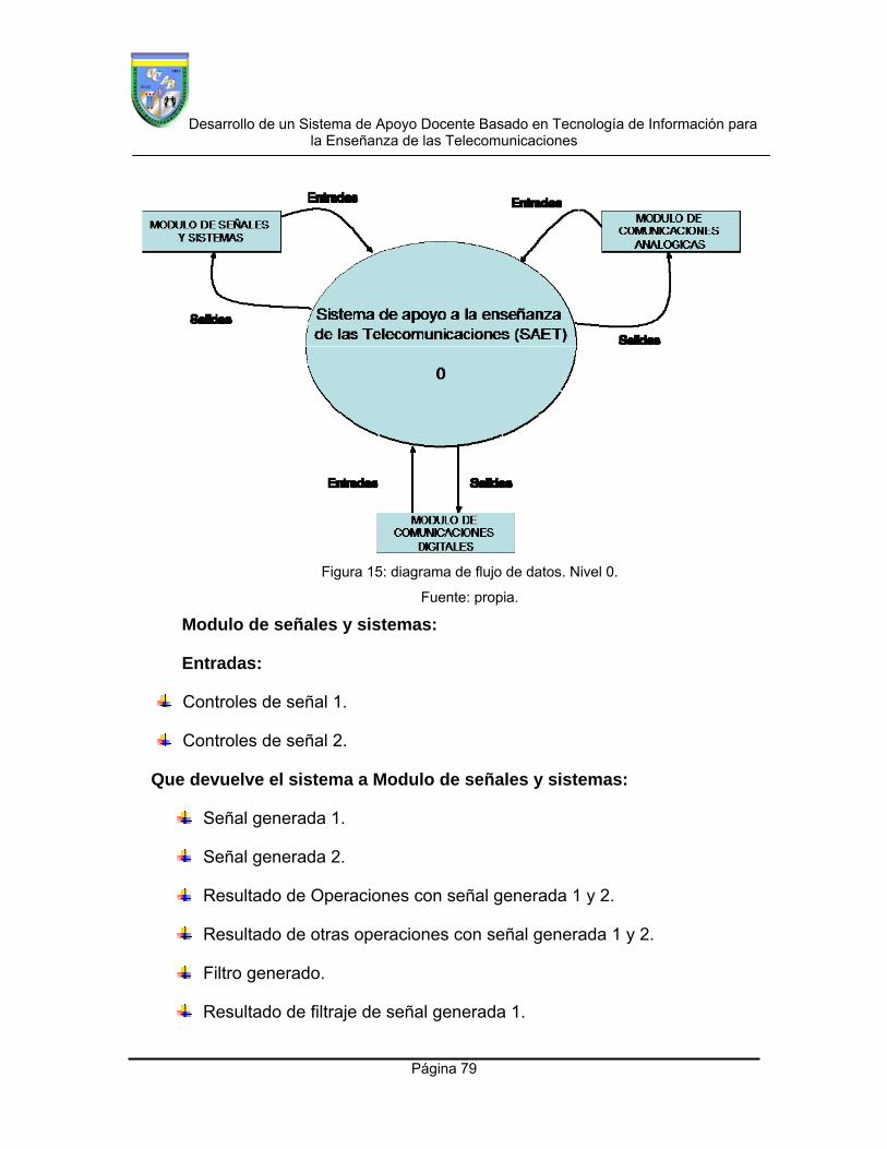
Desarrollo de un Sistema de Apoyo Docente Basado en Tecnología de Información para la Enseñanza de las Telecomunicaciones
Página 79
Figura 15: diagrama de flujo de datos. Nivel 0.
Fuente: propia.
Modulo de señales y sistemas:
Entradas:
Controles de señal 1.
Controles de señal 2.
Que devuelve el sistema a Modulo de señales y sistemas:
Señal generada 1.
Señal generada 2.
Resultado de Operaciones con señal generada 1 y 2.
Resultado de otras operaciones con señal generada 1 y 2.
Filtro generado.
Resultado de filtraje de señal generada 1.

Desarrollo de un Sistema de Apoyo Docente Basado en Tecnología de Información para la Enseñanza de las Telecomunicaciones
Página 80
Modulo de comunicaciones analógicas:
Entradas:
Controles de señal.
Que devuelve el sistema a Modulo de comunicaciones analógicas:
Señal generada.
Señal modulada analógicamente.
Resultado de caracterización de canal con la señal modulada.
Parámetros de canal
Resultado de detección de la señal modulada. Parámetros de
recepción.
Modulo de comunicaciones digitales:
Entradas:
Controles de señal.
Que devuelve el sistema a Modulo de comunicaciones analógicas:
Señal generada.
Señal modulada de forma binaria.
Resultado de caracterización de canal con la señal modulada.
Parámetros de canal
Resultado de detección de la señal modulada. Parámetros de
recepción.
Señal modulada de forma multinivel.

Desarrollo de un Sistema de Apoyo Docente Basado en Tecnología de Información para la Enseñanza de las Telecomunicaciones
Página 81
Curvas de probabilidad de error de señales moduladas de forma
binaria y multinivel.
En las siguientes figuras se muestra como es la interrelación de los
diferentes elementos del sistema SAET, las entradas y salidas que deben
generarse en los diferentes módulos.

Desarrollo de un Sistema de Apoyo Docente Basado en Tecnología de Información para la Enseñanza de las Telecomunicaciones
Página 82
Figura 16: Diagrama de Flujo de Datos. Nivel 1.
Fuente: propia.

Desarrollo de un Sistema de Apoyo Docente Basado en Tecnología de Información para la Enseñanza de las Telecomunicaciones
Página 83
Modulo de señales y
sistemas (MSS) Controles de señal 2Generación del mensaje
1
señal 1
señal 2
MSS operaciones Suma, resta,
multiplicación, division, normalizacio
n, DEP, IFFT, T. hilbert
2
señal 1
señal 2
FIN
Señal 1 Señal 2 Resultados
MSS operaciones
Convolucion Autocorrelac
ion Histograma
3
FIN
señal 1 señal 2
señal 1 señal 2
Señal 1 Señal 2 Resultados
MSS Filtraje
Selección de topología del
filtro 4
Selección del tipo de
filtro 5
señal 1
señal 1
señal 1 Topología seleccionada
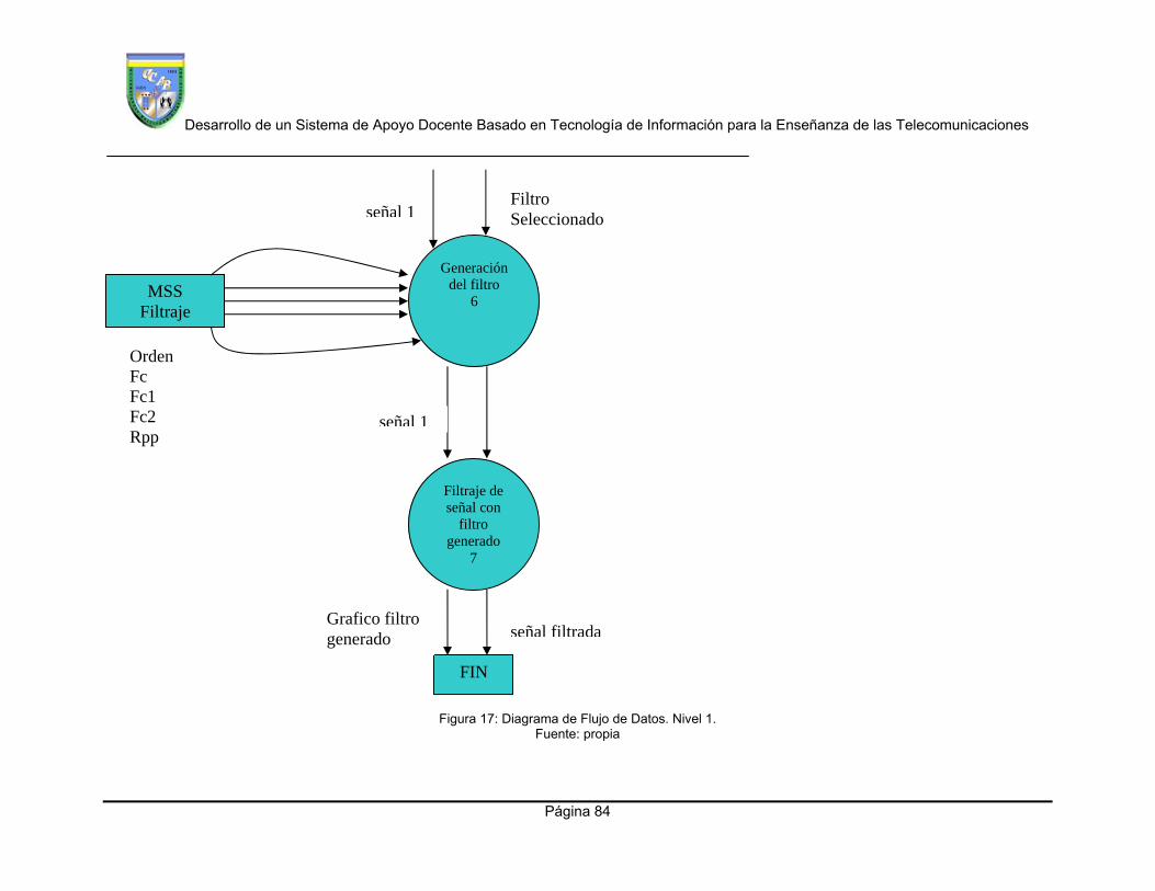
Desarrollo de un Sistema de Apoyo Docente Basado en Tecnología de Información para la Enseñanza de las Telecomunicaciones
Página 84
Figura 17: Diagrama de Flujo de Datos. Nivel 1. Fuente: propia
Generación del filtro
6
Filtro Seleccionado señal 1
MSS Filtraje
Orden Fc Fc1 Fc2 Rpp
Filtraje de señal con
filtro generado
7
señal 1
FIN
Grafico filtro generado señal filtrada

Desarrollo de un Sistema de Apoyo Docente Basado en Tecnología de Información para la Enseñanza de las Telecomunicaciones
Página 85
Modulo de Comunicaciones
Digitales
Controles Mensaje generado
MCD PCM
Mensaje generado
Parámetros Señal muestreada
Señal cuantificada
Generación del mensaje
(5)
muestreo
Parámetros cuantificación
Parámetros codificación
Cuantificación de la
señal (7)
FIN
Codificación de la señal
(8)
FIN Curvas
Velocidad Tx
PE
Señal codificada
Controles
MCD multinivel
Generación
Controles
Codificación
(2)
FIN
Señal generada
fase
Constelación
Modulación multinivel
(3)
Calculo
curvas PE (4)
FIN
Curvas PEIr a pag siguiente
*
Tomar Muestras
canal (6)

Desarrollo de un Sistema de Apoyo Docente Basado en Tecnología de Información para la Enseñanza de las Telecomunicaciones
Página 86
Figura 18: Diagrama de Flujo de Datos. Nivel 1.
Fuente: propia.

Desarrollo de un Sistema de Apoyo Docente Basado en Tecnología de Información para la Enseñanza de las Telecomunicaciones
Página 87
4.2.3 Requerimientos del sistema SAET
Los requerimientos del sistema son:
Generar, manipular, graficar y filtrar diferentes tipos de señales.
Generar, modular de forma analógica, simular una transmisión, recibir y
detectar diferentes tipos de señales. Además de calcular parámetros
de transmisión y de recepción.
Generar, convertir a digital, modular de forma digital, simular una
transmisión, recibir y detectar diferentes tipos de señales. Además de
dibujar curvas de PE y calcular parámetros de transmisión y de
recepción.
4.2.4 Carta estructurada de procesos
En la siguiente figura se muestra la carta estructurada de procesos con
las acciones que se deben generar en el sistema para generar la información
requerida por los usuarios.
Figura 19: Carta estructurada de procesos.
Fuente: propia.

Desarrollo de un Sistema de Apoyo Docente Basado en Tecnología de Información para la Enseñanza de las Telecomunicaciones
Página 88
4.2.5 Estructura General del Sistema de Apoyo a la Enseñanza de las
Telecomunicaciones (SAET)
En base a la información obtenida por los docentes para el desarrollo del
sistema se propone un modelo que proporcionara la información requerida en
cada una de las materias seleccionadas y adicionalmente será una fuente de
generación de conocimientos. El Sistema tiene diferentes módulos de
procesamiento de datos, con información que debe cruzarse entre los mismos,
ya que este sistema es de tipo secuencial.
Figura 21: Estructura del sistema propuesto.
Fuente: propia
Desarrollo de un Sistema de Apoyo Docente Basado en Tecnología de Información para la Enseñanza de las Telecomunicaciones
Página 89
4.2.6 Entradas, procesos y salidas del sistema SAET
Luego de presentar la estructura del sistema propuesto se procede a describir
las entradas, procesos y salidas del sistema SAET, en principio estas serán
mostradas de forma esquemática y separadas por sus correspondientes
módulos.

Desarrollo de un Sistema de Apoyo Docente Basado en Tecnología de Información para la Enseñanza de las Telecomunicaciones
Página 90
Modulo Entradas Procesos Salidas
Modulo de señales y
sistemas
Generación
Controles de señal 1:
Función (deterministica o aleatoria).
Forma de onda (seno, coseno, cuadrada, triangular, diente de sierra, voz, multitono seno y multitono coseno).
Amplitud (V).
Frecuencia (Hz).
Ciclo de trabajo (%).
Offset (V).
Fase (º)
Controles de señal 2:
Función (deterministica
Controles de señal 1:
Selección de la función a generar.
Selección de la forma de onda a generar
Asignación de amplitud de la onda a generar.
Asignación de frecuencia de la onda a generar.
Asignación de duración en tiempo de la onda cuadrada o triangular a generar.
Asignación de valor DC de la onda a generar.
Asignación de fase de la onda a generar.
Controles de señal 2:
Selección de la función a
Controles de señal 1:
Representación grafica en dominio del tiempo y dominio de la frecuencia de la señal escogida.
Controles de señal 2:

Desarrollo de un Sistema de Apoyo Docente Basado en Tecnología de Información para la Enseñanza de las Telecomunicaciones
Página 91
o aleatoria).
Forma de onda (seno, coseno, cuadrarda, triangular, diente de sierra, voz, multitono seno y multitono coseno).
Amplitud (V).
Frecuencia (Hz).
Ciclo de trabajo (%).
Offset (V).
Fase (º)
generar.
Selección de la forma de onda a generar
Asignación de amplitud de la onda a generar.
Asignación de frecuencia de la onda a generar.
Asignación de duración en tiempo de la onda cuadrada o triangular a generar.
Asignación de valor DC de la onda a generar.
Asignación de fase de la onda a generar.
Representación grafica en dominio del tiempo y dominio de la frecuencia de la señal escogida.
Modulo de señales y
sistemas
Operaciones
Señal escogida en controles de señal 1.
Señal escogida en control de señal 2.
Suma de Señal escogida en controles de señal 1 con Señal escogida en control de señal 2.
Resultado grafico de la Suma de Señal escogida en controles de señal 1 con Señal escogida en control de señal 2.
Resultado grafico de la resta

Desarrollo de un Sistema de Apoyo Docente Basado en Tecnología de Información para la Enseñanza de las Telecomunicaciones
Página 92
Resta de Señal escogida en controles de señal 1 con Señal escogida en control de señal 2.
Multiplicación de Señal escogida en controles de señal 1 con Señal escogida en control de señal 2.
División de Señal escogida en controles de señal 1 con Señal escogida en control de señal 2.
Normalización de Señal escogida en controles de señal 1.
Normalización de Señal escogida en control de señal 2.
Derivación de Señal escogida en controles de
de Señal escogida en controles de señal 1 con Señal escogida en control de señal 2.
Resultado grafico de la multiplicación de Señal escogida en controles de señal 1 con Señal escogida en control de señal 2.
Resultado grafico de la división de Señal escogida en controles de señal 1 con Señal escogida en control de señal 2.
Resultado grafico de la normalización de Señal escogida en controles de señal 1.
Resultado grafico de la normalización de Señal escogida en controles de señal 1.
Resultado grafico de la derivación de Señal escogida en controles de

Desarrollo de un Sistema de Apoyo Docente Basado en Tecnología de Información para la Enseñanza de las Telecomunicaciones
Página 93
señal 1.
Derivación de Señal escogida en control de señal 2.
Calculo de la DEP de Señal escogida en controles de señal 1.
Calculo de la DEP de Señal escogida en control de señal 2.
Calculo de la IFFT de Señal escogida en controles de señal 1.
Calculo de la IFFT de Señal escogida en control de señal 2.
Calculo de la transformada de hilbert de Señal escogida en controles de señal 1.
señal 1.
Resultado grafico de la derivación de Señal escogida en controles de señal 2.
Resultado grafico del cálculo de la DEP de la Señal escogida en controles de señal 1.
Resultado grafico del cálculo de la DEP de la Señal escogida en controles de señal 2.
Resultado grafico del cálculo de la IFFT de la Señal escogida en controles de señal 1.
Resultado grafico del cálculo de la IFFT de la Señal escogida en controles de señal 2.
Resultado grafico del cálculo de la transformada de hilbert de la Señal escogida en controles de señal 1.
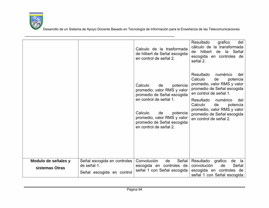
Desarrollo de un Sistema de Apoyo Docente Basado en Tecnología de Información para la Enseñanza de las Telecomunicaciones
Página 94
Calculo de la trasformada de hilbert de Señal escogida en control de señal 2.
Calculo de potencia promedio, valor RMS y valor promedio de Señal escogida en control de señal 1.
Calculo de potencia promedio, valor RMS y valor promedio de Señal escogida en control de señal 2.
Resultado grafico del cálculo de la transformada de hilbert de la Señal escogida en controles de señal 2.
Resultado numérico del Calculo de potencia promedio, valor RMS y valor promedio de Señal escogida en control de señal 1.
Resultado numérico del Calculo de potencia promedio, valor RMS y valor promedio de Señal escogida en control de señal 2.
Modulo de señales y
sistemas Otras
Señal escogida en controles de señal 1.
Señal escogida en control
Convolución de Señal escogida en controles de señal 1 con Señal escogida
Resultado grafico de la convolución de Señal escogida en controles de señal 1 con Señal escogida
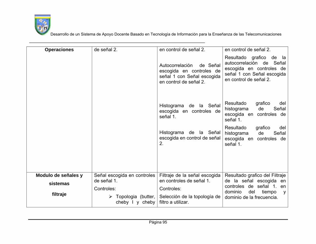
Desarrollo de un Sistema de Apoyo Docente Basado en Tecnología de Información para la Enseñanza de las Telecomunicaciones
Página 95
Operaciones de señal 2. en control de señal 2.
Autocorrelación de Señal escogida en controles de señal 1 con Señal escogida en control de señal 2.
Histograma de la Señal escogida en controles de señal 1.
Histograma de la Señal escogida en control de señal 2.
en control de señal 2.
Resultado grafico de la autocorrelación de Señal escogida en controles de señal 1 con Señal escogida en control de señal 2.
Resultado grafico del histograma de Señal escogida en controles de señal 1.
Resultado grafico del histograma de Señal escogida en controles de señal 1.
Modulo de señales y
sistemas
filtraje
Señal escogida en controles de señal 1.
Controles:
Topologia (butter, cheby I y cheby
Filtraje de la señal escogida en controles de señal 1.
Controles:
Selección de la topología de filtro a utilizar.
Resultado grafico del Filtraje de la señal escogida en controles de señal 1. en dominio del tiempo y dominio de la frecuencia.

Desarrollo de un Sistema de Apoyo Docente Basado en Tecnología de Información para la Enseñanza de las Telecomunicaciones
Página 96
II).
Tipo (pasabajos, pasaaltos, pasabanda y rechabanda).
Orden.
FC (Hz).
FC 1(Hz).
FC 2(Hz).
RPP
Selección del tipo de filtro a utilizar.
Asignación de orden del filtro a utilizar.
Asignación de frecuencia central del filtro a utilizar. (pasabajos o pasaaltos)
Asignación de frecuencia de corte inferior del filtro a utilizar. (pasabanda o rechabanda).
Asignación de frecuencia de corte superior del filtro a utilizar. (pasabanda o rechabanda).
Asignación de valor de rizado pico a pico del filtro a utilizar. (cheby I y cheby II )
Resultado grafico del tipo de filtro escogido en magnitud y fase. Diagrama de bode.
Tabla #3: Esquema de entradas, procesos y salidas del modulo de señales y sistemas.
Fuente: propia.

Desarrollo de un Sistema de Apoyo Docente Basado en Tecnología de Información para la Enseñanza de las Telecomunicaciones
Página 97
Modulo Entradas Procesos Salidas
Modulo de
Comunicaciones
Analógicas
Generación del
Mensaje
1.-Controles:
Tipo de señal
(seno,coseno,multito
no seno, multitono
coseno, voz).
Amplitud (V).
Frecuencia (Hz).
Fase (º).
Offset.
Numero de tonos:
2.
1.-Controles:
Selección de la forma de onda a generar.
Asignación de amplitud de la señal a generar.
Asignación de frecuencia de la señal a generar.
Asignación de fase de la señal a generar.
Asignación de nivel DC de la señal a generar.
Numero de tonos:
Selección del número de tonos secundarios a
1.-Controles:
Representación grafica en dominio del tiempo y dominio de la frecuencia de la señal escogida.

Desarrollo de un Sistema de Apoyo Docente Basado en Tecnología de Información para la Enseñanza de las Telecomunicaciones
Página 98
3.
4.
Parámetros tonos:
Amplitud de los tonos
(V).
Frecuencia de los
tonos (Hz).
generar.
Selección del número de tonos secundarios a generar.
Selección del número de
tonos secundarios a
generar.
Parámetros tonos:
Asignación de amplitud de los tonos secundarios de la señal a generar.
Asignación de frecuencias de los tonos secundarios de la señal a generar
Modulo de
Comunicaciones
Analógicas
Modulación
Señal escogida en modulo de comunicaciones analógicas generación.
Modula la Señal escogida en modulo de comunicaciones analógicas generación.
Representación grafica en dominio del tiempo y dominio de la frecuencia de la señal escogida en modulo de comunicaciones analógicas generación.
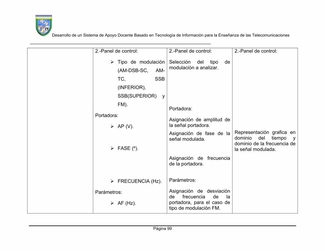
Desarrollo de un Sistema de Apoyo Docente Basado en Tecnología de Información para la Enseñanza de las Telecomunicaciones
Página 99
2.-Panel de control:
Tipo de modulación
(AM-DSB-SC, AM-
TC, SSB
(INFERIOR),
SSB(SUPERIOR) y
FM).
Portadora:
AP (V).
FASE (º).
FRECUENCIA (Hz).
Parámetros:
AF (Hz).
2.-Panel de control:
Selección del tipo de modulación a analizar.
Portadora:
Asignación de amplitud de la señal portadora.
Asignación de fase de la señal modulada.
Asignación de frecuencia de la portadora.
Parámetros:
Asignación de desviación de frecuencia de la portadora, para el caso de tipo de modulación FM.
2.-Panel de control:
Representación grafica en dominio del tiempo y dominio de la frecuencia de la señal modulada.
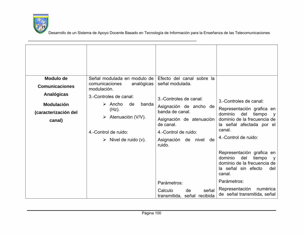
Desarrollo de un Sistema de Apoyo Docente Basado en Tecnología de Información para la Enseñanza de las Telecomunicaciones
Página 100
Modulo de
Comunicaciones
Analógicas
Modulación
(caracterización del
canal)
Señal modulada en modulo de comunicaciones analógicas modulación.
3.-Controles de canal:
Ancho de banda (Hz).
Atenuación (V/V).
4.-Control de ruido:
Nivel de ruido (v).
Efecto del canal sobre la señal modulada.
3.-Controles de canal:
Asignación de ancho de banda de canal.
Asignación de atenuación de canal.
4.-Control de ruido:
Asignación de nivel de ruido.
Parámetros:
Calculo de señal transmitida, señal recibida
3.-Controles de canal:
Representación grafica en dominio del tiempo y dominio de la frecuencia de la señal afectada por el canal.
4.-Control de ruido:
Representación grafica en dominio del tiempo y dominio de la frecuencia de la señal sin efecto del canal.
Parámetros:
Representación numérica de señal transmitida, señal

Desarrollo de un Sistema de Apoyo Docente Basado en Tecnología de Información para la Enseñanza de las Telecomunicaciones
Página 101
y relación señal a ruido recibida.
recibida y relación señal a ruido recibida.
Modulo de
Comunicaciones
Analógicas
Detección de la señal
Señal afectada por el canal o señal sin efecto de canal.
5.-Controles de detección:
Tipo de
demodulación: (AM-
DSB-SC, AM-TC,
SSB (INFERIOR),
SSB (SUPERIOR) y
FM).
Tipo de detección (detección sincronía o detección de envolvente).
Control pasabanda:
FC1 (Hz).
Detección de la señal afectada por el canal o detección de la señal sin efecto del canal.
5.-Controles de detección:
Selección del tipo de demodulación a ejecutar.
Selección del tipo de detección a utilizar (solo aplica para el caso de AM-TC).
Representación grafica en dominio del tiempo y dominio de la frecuencia de la señal afectada por el canal o de la señal sin efecto del canal.
Control pasabanda:
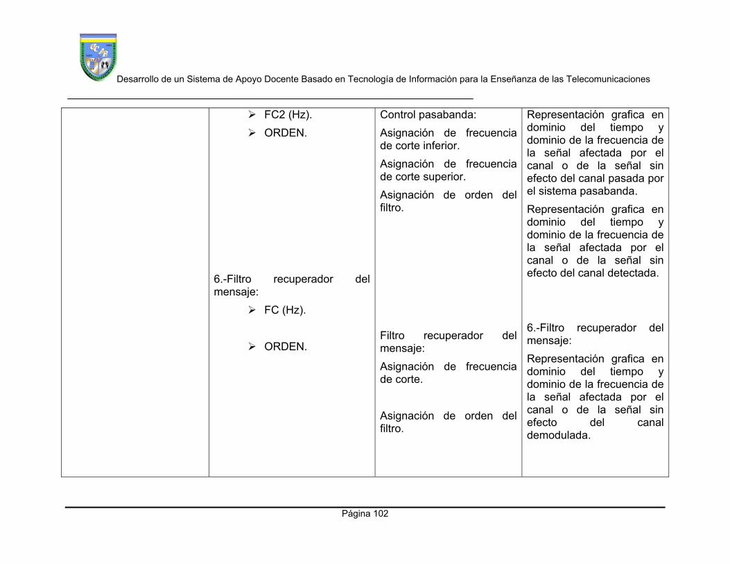
Desarrollo de un Sistema de Apoyo Docente Basado en Tecnología de Información para la Enseñanza de las Telecomunicaciones
Página 102
FC2 (Hz).
ORDEN.
6.-Filtro recuperador del mensaje:
FC (Hz).
ORDEN.
Control pasabanda:
Asignación de frecuencia de corte inferior.
Asignación de frecuencia de corte superior.
Asignación de orden del filtro.
Filtro recuperador del mensaje:
Asignación de frecuencia de corte.
Asignación de orden del filtro.
Representación grafica en dominio del tiempo y dominio de la frecuencia de la señal afectada por el canal o de la señal sin efecto del canal pasada por el sistema pasabanda.
Representación grafica en dominio del tiempo y dominio de la frecuencia de la señal afectada por el canal o de la señal sin efecto del canal detectada.
6.-Filtro recuperador del mensaje:
Representación grafica en dominio del tiempo y dominio de la frecuencia de la señal afectada por el canal o de la señal sin efecto del canal demodulada.

Desarrollo de un Sistema de Apoyo Docente Basado en Tecnología de Información para la Enseñanza de las Telecomunicaciones
Página 103
Parámetros de recepción:
Representación numérica de señal detectada y relación señal a ruido detectada.
Tabla # 4: Esquema de entradas, procesos y salidas del modulo de comunicaciones analógicas.
Fuente: propia.
Modulo Entradas Procesos Salidas
Modulo de
Comunicaciones
digitales
Generación del
Mensaje
Controles:
Tipo de señal
(seno,coseno,multito
no seno, multitono
coseno, voz).
Amplitud (V).
Frecuencia (Hz).
Fase (º).
Controles:
Selección de la forma de onda a generar.
Asignación de amplitud de la señal a generar.
Asignación de frecuencia
Controles:
Representación grafica en dominio del tiempo y dominio de la frecuencia de la señal escogida.

Desarrollo de un Sistema de Apoyo Docente Basado en Tecnología de Información para la Enseñanza de las Telecomunicaciones
Página 104
Offset.
Numero de tonos:
2.
3.
4.
Parámetros tonos:
Amplitud de los tonos
(V).
de la señal a generar.
Asignación de fase de la señal a generar.
Asignación de nivel DC de la señal a generar.
Numero de tonos:
Selección del número de tonos secundarios a generar.
Selección del número de tonos secundarios a generar.
Selección del número de
tonos secundarios a
generar.
Parámetros tonos:
Asignación de amplitud de

Desarrollo de un Sistema de Apoyo Docente Basado en Tecnología de Información para la Enseñanza de las Telecomunicaciones
Página 105
Frecuencia de los
tonos (Hz).
los tonos secundarios de la señal a generar.
Asignación de frecuencias de los tonos secundarios de la señal a generar
Modulo de
Comunicaciones
digitales
modulación PCM
Señal generada en modulo de comunicaciones digitales generación del mensaje.
Parámetros de muestreo:
Amplitud de la señal muestreadota (V).
Frecuencia de la señal muestreadota (Hz).
Ciclo de trabajo de la señal mustreadora (%).
Parámetros de cuantificación:
Numero de
Digitalización de la Señal generada en modulo de comunicaciones digitales generación del mensaje.
Parámetros de muestreo:
Asignación de amplitud de la señal muestreadora.
Asignación de amplitud de frecuencia de la señal muestreadota.
Asignación de duración en tiempo de la señal muestreadora.
Parámetros de cuantificación:
Representación grafica en dominio del tiempo y dominio de la frecuencia de la señal escogida.
Parámetros de muestreo:
Representación grafica en dominio del tiempo y dominio de la frecuencia de la señal muestreada.
Parámetros de

Desarrollo de un Sistema de Apoyo Docente Basado en Tecnología de Información para la Enseñanza de las Telecomunicaciones
Página 106
bit/muestra.
Compansión:
Ley U.
Parámetros de codificación:
Códigos de línea (UNIPOLAR NRZ, UNIPOLAR RZ, POLAR NRZ, POLAR RZ, BIPOLAR NRZ, BIPOLAR RZ y MANCHESTER).
Asignación de número de bit para la codificación de la señal.
Compansión:
Activación de compansión utilizando ley u.
Parámetros de codificación:
Selección del código de línea a utilizar.
cuantificación:
Representación grafica en dominio del tiempo y dominio de la frecuencia de la señal cuantificada.
Representación numérica de potencia del error de cuantificación y los niveles de cuantificación.
Parámetros de codificación:
Representación grafica en dominio del tiempo y dominio de la frecuencia de la señal codificada.
Modulo de
Comunicaciones
digitales
Modulación
Señal escogida en modulo de comunicaciones digitales generación.
Panel de control:
Tipo de modulación
Modula la Señal escogida en modulo de comunicaciones digitales generación.
Panel de control:
Selección del tipo de
Representación grafica en dominio del tiempo y dominio de la frecuencia de la señal escogida en modulo de comunicaciones analógicas generación.
Panel de control:

Desarrollo de un Sistema de Apoyo Docente Basado en Tecnología de Información para la Enseñanza de las Telecomunicaciones
Página 107
(ASK, FSK Y PSK).
Portadora:
AP (V).
FASE (º).
FRECUENCIA (Hz).
Parámetros:
AF (Hz).
modulación a analizar.
Portadora:
Asignación de amplitud de la señal portadora.
Asignación de fase de la señal modulada.
Asignación de frecuencia de la portadora.
Parámetros:
Asignación de desviación de frecuencia de la portadora, para el caso de tipo de modulación FSK.
Representación grafica en dominio del tiempo y dominio de la frecuencia de la señal modulada.
Representación grafica del diagrama de constelación de la señal modulada.

Desarrollo de un Sistema de Apoyo Docente Basado en Tecnología de Información para la Enseñanza de las Telecomunicaciones
Página 108
Modulo de
Comunicaciones
digitales
Modulación
(caracterización del
canal)
Señal modulada en modulo de comunicaciones digitales modulación.
Controles de canal:
Ancho de banda (Hz).
Atenuación (V/V).
Control de ruido:
Nivel de ruido (v).
Efecto del canal sobre la señal modulada.
Controles de canal:
Asignación de ancho de banda de canal.
Asignación de atenuación de canal.
Control de ruido:
Asignación de nivel de ruido.
Representación grafica en dominio del tiempo y dominio de la frecuencia de la señal afectada por el canal.
Representación grafica en dominio del tiempo y dominio de la frecuencia de la señal sin efecto del canal.
Parámetros:
Representación numérica de señal transmitida, señal recibida y relación señal a ruido recibida.
Representación grafica del diagrama de constelación de la señal modulada.

Desarrollo de un Sistema de Apoyo Docente Basado en Tecnología de Información para la Enseñanza de las Telecomunicaciones
Página 109
Modulo de
Comunicaciones
digitales
Detección de la señal
Señal afectada por el canal o señal sin efecto de canal.
Controles de detección:
Tipo de
demodulación: (ASK,
FSK Y PSK).
Tipo de detección (detección coherente o detección no coherente).
Control pasabanda:
FC1 (Hz).
FC2 (Hz).
ORDEN.
Detección de la señal afectada por el canal o detección de la señal sin efecto del canal.
Controles de detección:
Selección del tipo de demodulación a ejecutar.
Selección del tipo de detección a utilizar (solo aplica para el caso de AM-TC).
Control pasabanda:
Asignación de frecuencia de corte inferior.
Asignación de frecuencia de corte superior.
Asignación de orden del filtro.
Representación grafica en dominio del tiempo y dominio de la frecuencia de la señal afectada por el canal o de la señal sin efecto del canal.
Control pasabanda:
Representación grafica en dominio del tiempo y dominio de la frecuencia de la señal afectada por el canal o de la señal sin efecto del canal pasada por el sistema pasabanda.
Representación grafica en
Desarrollo de un Sistema de Apoyo Docente Basado en Tecnología de Información para la Enseñanza de las Telecomunicaciones
Página 110
Control pasabanda2:
FC1 (Hz).
FC2 (Hz).
ORDEN.
Control pasabanda2:
Asignación de frecuencia de corte inferior.
Asignación de frecuencia de corte superior.
Asignación de orden del filtro.
dominio del tiempo y dominio de la frecuencia de la señal afectada por el canal o de la señal sin efecto del canal detectada.
Control pasabanda 2:
Representación grafica en dominio del tiempo y dominio de la frecuencia de la señal afectada por el canal o de la señal sin efecto del canal pasada por el sistema pasabanda.
Representación grafica en dominio del tiempo y dominio de la frecuencia de la señal afectada por el canal o de la señal sin efecto del canal detectada.
Desarrollo de un Sistema de Apoyo Docente Basado en Tecnología de Información para la Enseñanza de las Telecomunicaciones
Página 111
Filtro recuperador del mensaje:
FC (Hz).
ORDEN.
Filtro recuperador del mensaje:
Asignación de frecuencia de corte.
Asignación de orden del filtro.
Filtro recuperador del mensaje:
Representación grafica en dominio del tiempo y dominio de la frecuencia de la señal afectada por el canal o de la señal sin efecto del canal demodulada.
Parámetros de recepción:
Representación numérica de señal detectada y la probabilidad de error.
Representación grafica de las curvas de probabilidad de error teóricas y practicas.

Desarrollo de un Sistema de Apoyo Docente Basado en Tecnología de Información para la Enseñanza de las Telecomunicaciones
Página 112
Modulo de
Comunicaciones
digitales
modulación
multinivel
Controles:
Tipo (QPSK, 8-PSK, 16-PSK, 4-QAM, 8-QAM, 16-QAM, 32-QAM y 64-QAM).
Numero de bit.
Rb.
Nivel de ruido.
Controles:
Selección del tipo de modulación a ejecutar.
Asignación de número de bit a utilizar.
Asignación de tasa de codificación de bit a utilizar.
Asignación de nivel de ruido del canal.
Controles:
Representación grafica en dominio del tiempo de la señal codificada.
Representación grafica en dominio del tiempo de la señal recodificada.
Representación grafica en dominio del tiempo de la señal parcialmente modulada.
Representación grafica en dominio del tiempo de la señal modulada.
Representación grafica en dominio de la frecuencia de la señal modulada.
Representación grafica de las curvas de PE teóricas y

Desarrollo de un Sistema de Apoyo Docente Basado en Tecnología de Información para la Enseñanza de las Telecomunicaciones
Página 113
practicas.
Representación numérica de las fases de la señal modulada.
Tabla # 5: Esquema de entradas, procesos y salidas del modulo de comunicaciones digitales.
Fuente: propia.

Desarrollo de un Sistema de Apoyo Docente Basado en Tecnología de Información para la Enseñanza de las Telecomunicaciones
Página 114
4.2.7 Programación y pruebas
A continuación serán presentadas las pantallas en secuencia ordenada del
sistema SAET, con las cuales se cumple el objetivo de representar los
resultados de la simulación de manera fácil y comprensible, que a su vez permita
la interacción de forma amigable y didáctica con el usuario, los algoritmos y
códigos fuente del sistema serán presentados en los anexos.
Figura 22: Pantalla inicial sistema SAET.
Fuente: propia.

Desarrollo de un Sistema de Apoyo Docente Basado en Tecnología de Información para la Enseñanza de las Telecomunicaciones
Página 115
Figura 23: Modulo de señales y sistemas del sistema SAET.
Fuente: propia.
Figura 24: Modulo de señales y sistemas generación, del sistema SAET.
Fuente: propia.

Desarrollo de un Sistema de Apoyo Docente Basado en Tecnología de Información para la Enseñanza de las Telecomunicaciones
Página 116
Figura 25: Modulo de señales y sistemas operaciones, del sistema SAET.
Fuente: propia.
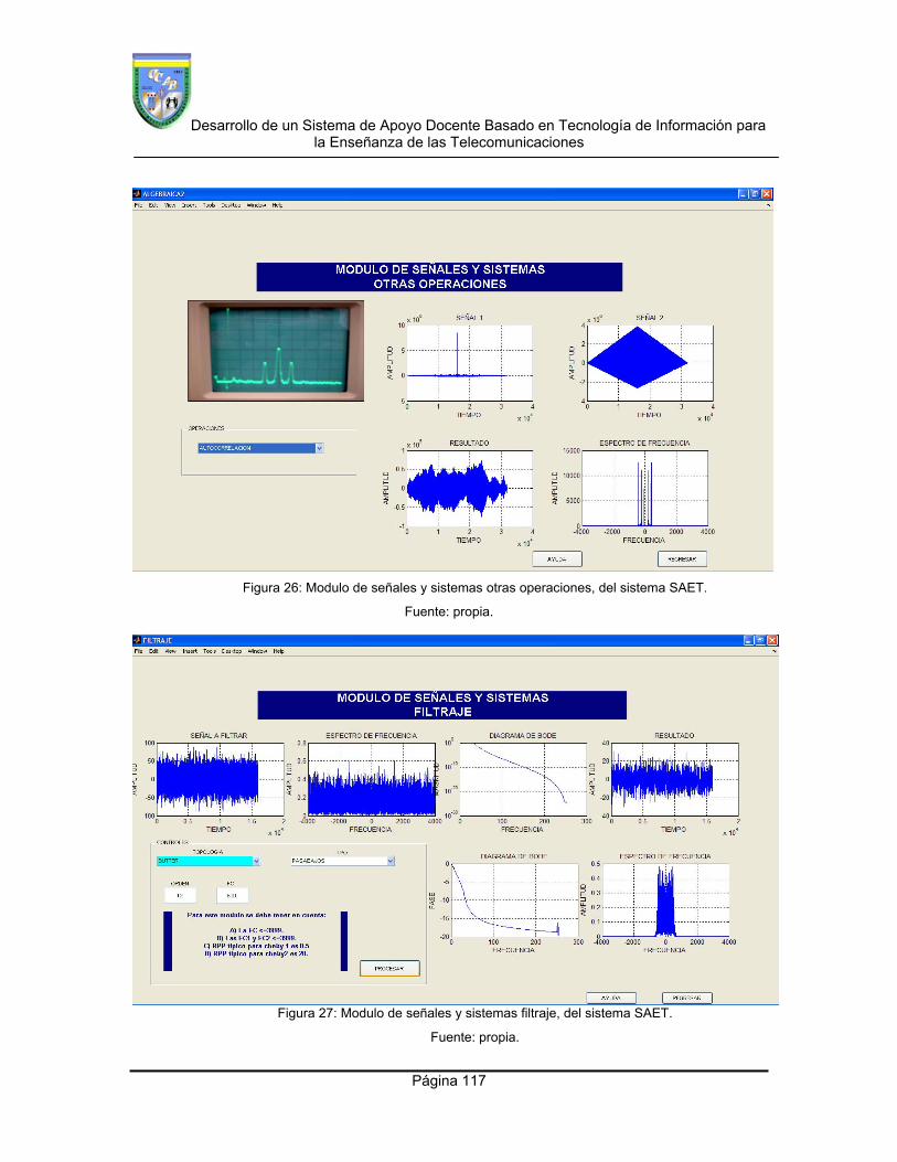
Desarrollo de un Sistema de Apoyo Docente Basado en Tecnología de Información para la Enseñanza de las Telecomunicaciones
Página 117
Figura 26: Modulo de señales y sistemas otras operaciones, del sistema SAET.
Fuente: propia.
Figura 27: Modulo de señales y sistemas filtraje, del sistema SAET.
Fuente: propia.

Desarrollo de un Sistema de Apoyo Docente Basado en Tecnología de Información para la Enseñanza de las Telecomunicaciones
Página 118
Figura 28: Modulo de comunicaciones analógicas del sistema SAET.
Fuente: propia.
Figura 29: Modulo de comunicaciones analógicas generación del mensaje, del sistema SAET.
Fuente: propia.

Desarrollo de un Sistema de Apoyo Docente Basado en Tecnología de Información para la Enseñanza de las Telecomunicaciones
Página 119
Figura 30: Modulo de comunicaciones analógicas modulación, del sistema SAET.
Fuente: propia.
Figura 31: Modulo de comunicaciones analógicas modulación caracterización del canal, del sistema SAET.
Fuente: propia.

Desarrollo de un Sistema de Apoyo Docente Basado en Tecnología de Información para la Enseñanza de las Telecomunicaciones
Página 120
Figura 32: Modulo de comunicaciones analógicas detección de la señal, del sistema SAET.
Fuente: propia.
Figura 33: Modulo de comunicaciones digitales del sistema SAET.
Fuente: propia.
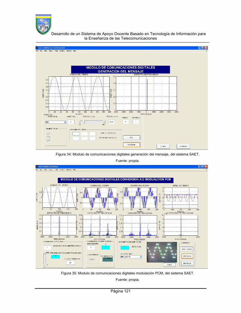
Desarrollo de un Sistema de Apoyo Docente Basado en Tecnología de Información para la Enseñanza de las Telecomunicaciones
Página 121
Figura 34: Modulo de comunicaciones digitales generación del mensaje, del sistema SAET.
Fuente: propia.
Figura 35: Modulo de comunicaciones digitales modulación PCM, del sistema SAET.
Fuente: propia.

Desarrollo de un Sistema de Apoyo Docente Basado en Tecnología de Información para la Enseñanza de las Telecomunicaciones
Página 122
Figura 36: Modulo de comunicaciones digitales compansión, del sistema SAET.
Fuente: propia.
Figura 37: modulo de comunicaciones digitales codificación PCM, del sistema SAET.
Fuente: propia.
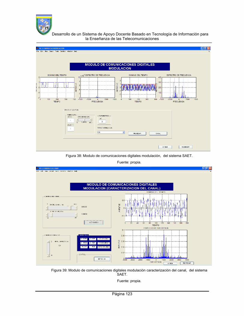
Desarrollo de un Sistema de Apoyo Docente Basado en Tecnología de Información para la Enseñanza de las Telecomunicaciones
Página 123
Figura 38: Modulo de comunicaciones digitales modulación, del sistema SAET.
Fuente: propia.
Figura 39: Modulo de comunicaciones digitales modulación caracterización del canal, del sistema SAET.
Fuente: propia.

Desarrollo de un Sistema de Apoyo Docente Basado en Tecnología de Información para la Enseñanza de las Telecomunicaciones
Página 124
Figura 40: Modulo de comunicaciones digitales detección de la señal, del sistema SAET.
Fuente: propia.
Figura 41: Modulo de comunicaciones digitales curvas de PE del sistema SAET.
Fuente: propia.

Desarrollo de un Sistema de Apoyo Docente Basado en Tecnología de Información para la Enseñanza de las Telecomunicaciones
Página 125
Figura 42: Modulo de comunicaciones digitales modulación multinivel, del sistema SAET.
Fuente: propia.
Figura 43: Modulo de comunicaciones digitales modulación multinivel curvas de PE, del sistema SAET.
Fuente: propia.

Desarrollo de un Sistema de Apoyo Docente Basado en Tecnología de Información para la Enseñanza de las Telecomunicaciones
Página 126
CAPITULO V
5. CONCLUSIONES
Finalmente se puede decir que se cumplieron con los siguientes objetivos:
Se establecieron las estrategias que enmarcaran el proceso de
enseñanza-aprendizaje en el campo de las telecomunicaciones,
resultando una combinación de diferentes enfoques, donde predominó
el enfoque conductista y el constructivista.
Luego de establecer las estrategias didácticas de enseñanza, estas
fueron tomadas en cuenta en el diseño de la herramienta.
Se recopilaron los contenidos relevantes en las diferentes cátedras de
la carrera de ingeniería de telecomunicaciones. Dichos contenidos
fueron seleccionados en base a su complejidad técnica y matemática,
los mismos fueron descritos en el desarrollo de la propuesta.
Se desarrolló el sistema de computación para la simulación de
señales analógicas y digitales relacionado con los contenidos
seleccionados, describiendo los procesos de análisis y diseño del
mismo.
Se logro representar los resultados de la simulación de manera fácil y
comprensible mediante la implantación del sistema SAET, permitiendo
la interacción de forma amigable y didáctica con el usuario.
En la actualidad, las herramientas de simulación programables se revelan
como las más eficaces y adecuadas para apoyar el proceso de enseñanza
aprendizaje de las telecomunicaciones ya que permite plantear escenarios
muy parecidos a la realidad, además que permite realizar cambios para
analizar diferentes situaciones.

Desarrollo de un Sistema de Apoyo Docente Basado en Tecnología de Información para la Enseñanza de las Telecomunicaciones
Página 127
El desarrollo de un Sistema de Apoyo a la Enseñanza de
Telecomunicaciones para la Escuela de Ingeniería de Telecomunicaciones
contribuye al mejoramiento de la formación del recurso humano en las áreas
seleccionadas para el desarrollo de la herramienta.
Las Tecnologías de Información y comunicación (TIC), constituyen
elementos muy importantes en la adquisición y transferencia de
conocimiento, su implementación y desarrollo contribuye cada vez más al
fortalecimiento del conocimiento en las universidades.
5.1 RECOMENDACIONES
Se recomienda continuar con el desarrollo de la herramienta SAET, ya
que los temas y tópicos seleccionados solo representan un pequeño
porcentaje del universo de conocimiento e información del área de las
telecomunicaciones.
Específicamente se pueden desarrollar sistemas SAET enfocados en
áreas como antenas, microondas, líneas de transmisión, sistema móviles
celulares, sistemas de transmisión por fibra óptica, sistemas de audio y video
y sistemas satelitales.

Desarrollo de un Sistema de Apoyo Docente Basado en Tecnología de Información para la Enseñanza de las Telecomunicaciones
Página 128
REFERENCIAS BIBLIOGRAFICAS
Balestrini Miriam. Como se elabora un proyecto de investigación. 2002. Sexta
edición. Consultores y asociados.
Borje Langerfors, Teoría de los Sistemas de Información. 1985. “El Ateneo”, 305
Pág.
Carlson Bruce, Communication System. 2002. Cuarta Edición. McGraw-Hill, 793
Pág.
Cintrón F. Carmen R. Guía de introducción a la gerencia de sistemas de
información. 2001.
Del Rosario, Zuleima. Guía para la elaboración de reportes de investigación.
UCAB 2006.
Dibut, L., Valdés, G., Arteaga, H. & all (1998). Las nuevas tecnologías de la
información y la comunicación como mediadoras del proceso enseñanza-
aprendizaje.
Efraim Turban, Decision Support Systems and Intelligent Systems, Prentice Hall,
1998. Cap. 1.
Ertmer, P y Newby T. (1993). Conductismo, cognitivismo y constructivismo: una
comparación de los aspectos críticos desde la perspectiva del diseño de
instrucción. Traducción de Ferstadt, N. y Mario Szcaurek, M. Universidad
Pedagógica Experimental Libertador. Instituto Pedagógico de Caracas.
Desarrollo de un Sistema de Apoyo Docente Basado en Tecnología de Información para la Enseñanza de las Telecomunicaciones
Página 129
Gutierrez, R. y Pinto, R., Models and Simulations. Construction of a Theoretically
Grounded Analytic Instrument. En: E. Mechlová (ed), Proceedings of the GIREP
2004 International Conference Teaching and Learning Physics in New Contexts.
Selected Papers. Ostrava, Czech Republic: University of Ostrava, p. 157-158.
James A. Senn, Análisis y diseno de sistemas de información. McGaw-Hill. 1987.
619 Pág.
Laudon P.Jane, Administración de los Sistemas de Información. Tercera Edición.
Pretince Hall. 2001. 881 Pág.
Ramírez, Jesús. Análisis y Diseño de Sistemas de Información. Guía de clases
del Postgrado de Sistemas de Información de la UCAB, no publicada.
Rosas, Mirna.Guía Práctica de Investigación. 2002. Editorial Trillas.
Sampieri R. Collado C. Lucio P. Metodología de la investigación. 1998. Segunda
edicion.. McGraw Hill.
Stremler F.G, Introducción a los Sistemas de Comunicación. 1993. Tercera
Edicion. Pearson, 755 Pág.
Zamarro, J.M.; Martín, E.; Esquembre, F. y Härtel, H (1998) Unidades didácticas
en Física utilizando simulaciones interactivas controladas desde ficheros HTML.
Comunicación IV Congreso RIBIE, Brasilia.
.

Anexos
Programas de las materias seleccionadas para el desarrollo del sistema SAET.
UNIVERSIDAD CATOLICA ANDRES BELLO Urb. Montalbán - La Vega - Apartado 29068
Teléfono: 442-9511 Fax: 471-3043 Caracas, 1021 - Venezuela
Facultad de Ingeniería Escuela de Ingeniería de Telecomunicaciones
Asignatura: SEÑALES Y SISTEMAS I Vigente desde: Octubre 2004 Horas semanales Unidades Período Teoría Práctica Laboratorio de crédito 5 4 2 0 5 Requisitos Cálculo IV, Probabilidades y procesos Estocásticos, Circuitos y sistemas electrónicos II Justificación del programa El problema de transmitir una señal de un punto a otro utilizando un Sistema de Comunicaciones, implica poder caracterizar diferentes tipos de señales en diferentes dominios y aprender a utilizar herramientas que permitan calcular el efecto de sistemas, lineales y no lineales, sobre las señales que los alimentan. Para esto se hace necesario definir criterios específicos de comportamiento como potencia, ancho de banda, relación entre potencias, etc. El curso de Señales y Sistemas ofrece las herramientas para lograr estos propósitos. Esto incluye no solo la asimilación de conceptos teóricos sino el manejo de simuladores de sistemas de comunicaciones. Objetivos del aprendizaje Al finalizar el curso de Señales y Sistemas I: El estudiante dominará diversas herramientas temporales y frecuenciales que le permitirán calcular parámetros específicos de las señales y resolver el problema del paso de señales determinísticas y aleatorias continuas por sistemas lineales y no lineales, los cuales conformarían un sistema de comunicaciones eléctricas. El estudiante se familiarizará con un simulador que le permitirá verificar los conceptos teóricos cubiertos en clases y además diseñar nuevos sistemas y estudiar su comportamiento a la luz de criterios previamente definidos. El estudiante mejorará sus habilidades de trabajo en equipo y de expresión oral a través de: a) la aplicación de talleres de problemas en clases dirigidos por el profesor, b) del desarrollo de un proyecto de investigación y c) la realización de prácticas semanales de laboratorio; en todos los casos deberá trabajar en equipo y además, en los dos primeros, debe prepararse para la presentación y defensa pública de la actividad asignada. El estudiante tendrá la posibilidad de mejorar parcialmente sus habilidades de expresión escrita ya que se le asignará un informe de alguna de las prácticas que desarrollará a lo largo del semestre y el mismo será examinado detalladamente y corregido por el profesor. Contenido Programático CAPITULO I: INTRODUCCIÓN. Elementos de un sistema de Comunicaciones Eléctricas: Transductor de entrada, Transmisor, canal, Receptor, Transductor de salida. Ruido, Interferencia y Distorsión. CAPITULO II: SEÑALES Y SISTEMAS: Clasificación de señales y Sistemas. Señales determinísticas y aleatorias, de energía o de potencia, periódicas y no-periódicas. Sistemas Lineales y no Lineales, invariantes y variantes en el tiempo, causales y no causales. Señales sinusoidales: representación temporal, espectral y fasorial. Respuesta de Sistemas Lineales e Invariantes en el tiempo (LIT) a sinusoides. Respuesta en frecuencia. Señales especiales: Delta Dirac, escalón, Sinc. CAPITULO III: ANALISIS TEMPORAL DE SEÑALES Y SISTEMAS Representación de un sistema continúo mediante ecuaciones diferenciales de coeficientes constantes: Solución homogénea y particular. Respuesta al impulso y respuesta en frecuencia. Representación de un sistema continúo mediante su respuesta al impulso. Convolución continúa. CAPITULO IV: ANALISIS EN FRECUENCIA DE SEÑALES Y SISTEMAS CONTINUOS: Series de Fourier: Representación generalizada de una función en serie de Fourier.
Serie Trigonométrica y exponencial de Fourier. Propiedades de las series de Fourier. Paso de una señal periódica por un sistema LIT. Teorema de Parseval. Transformada de Fourier: Definición, condiciones de existencia y propiedades. Teorema de Rayleigh. Paso de una señal no periódica por un sistema LIT. CAPITULO V: PROCESOS ALEATORIOS Y RUIDO: Repaso de: Funciones de Densidad de Probabilidad, Promedios Estadísticos, Modelos Probabilísticos. Procesos Aleatorios: Estacionaridad, Ergodicidad, Autocorrelación, Densidad Espectral de Potencia (DEP). Paso de señales aleatorias a través de sistemas lineales. Ruido Térmico, Ruido Blanco. Ruido. Distorsión lineal. Sistema Bandabase contaminado con Ruido Blanco gaussiano. Repetidoras. Estrategias metodológicas - Exposición del profesor en el salón de clases. - Interacción del estudiante con el profesor y su compañero de equipo en el laboratorio a través de la realización de experiencias prácticas asociadas a la teoría. - Familiarización con herramientas de simulación propias del área de comunicaciones a través de prácticas guiadas y desarrollo de proyectos. - Realización de talleres de problemas en los cuales los estudiantes son agrupados y se les asigna, a cada equipo, un problema específico y distinto el cual deben resolver y posteriormente exponer al resto del grupo en el salón de clases. - Realización de un informe sobre una de las prácticas de laboratorio para mejorar sus capacidades de expresión escrita y de realización de informes técnicos. - Desarrollo de un proyecto de investigación con aplicaciones prácticas para mejorar su metodología de investigación y sus habilidades de trabajo en equipo. - Exposición del proyecto de investigación para mejorar sus capacidades de expresión oral. Tiempo estimado: El programa se cubre en 15 semanas. Cada semana se cubren tópicos de teoría (4 h/semana) y se realiza una práctica de 2 horas. Se realizan 3 talleres de problemas durante todo el semestre. El proyecto se expone en las últimas dos sesiones de laboratorio . Estrategia de Evaluación: La evaluación incluye: Tres exámenes parciales con un porcentaje de 23%, 26% y 32% respectivamente.En el segundo y tercer parcial se incluyen preguntas de laboratorio. Ejecución de las prácticas 5% Trabajo de Investigación (Proyecto) con un peso de 9% Informe sobre una práctica de laboratorio 5% Bibliografía: ALAN OPPENHEIM y ALAN WILSKY. Señales y Sistemas. Segunda Edición.. Prentice Hall.1997. SIMON HAYKIN y BARRY VAN VEEN. Señales y Sistemas. Limusa-Wiley. 2001. ROBERT GABEL & RICHARD ROBERTS.Signals and Linear Systems. Third Edition. John Wiley.1987. TRINA ADRIAN DE PEREZ. Material disponible en Módulo 7-UCAB; Apuntes de la asignatura Elaborados por la profesora Trina Adrián de Pérez. 2003.
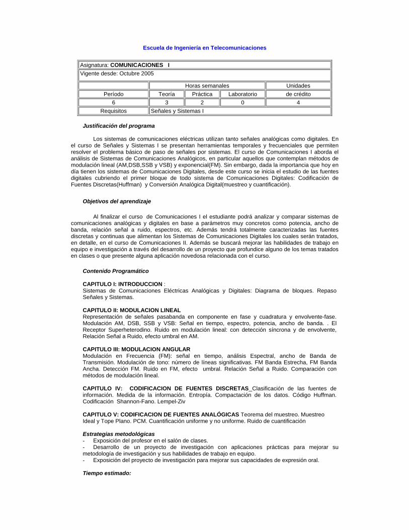
Escuela de Ingeniería en Telecomunicaciones
Asignatura: COMUNICACIONES I
Vigente desde: Octubre 2005
Horas semanales Unidades
Período Teoría Práctica Laboratorio de crédito
6 3 2 0 4
Requisitos Señales y Sistemas I
Justificación del programa
Los sistemas de comunicaciones eléctricas utilizan tanto señales analógicas como digitales. En el curso de Señales y Sistemas I se presentan herramientas temporales y frecuenciales que permiten resolver el problema básico de paso de señales por sistemas. El curso de Comunicaciones I aborda el análisis de Sistemas de Comunicaciones Analógicos, en particular aquellos que contemplan métodos de modulación lineal (AM,DSB,SSB y VSB) y exponencial(FM). Sin embargo, dada la importancia que hoy en día tienen los sistemas de Comunicaciones Digitales, desde este curso se inicia el estudio de las fuentes digitales cubriendo el primer bloque de todo sistema de Comunicaciones Digitales: Codificación de Fuentes Discretas(Huffman) y Conversión Analógica Digital(muestreo y cuantificación).
Objetivos del aprendizaje
Al finalizar el curso de Comunicaciones I el estudiante podrá analizar y comparar sistemas de comunicaciones analógicas y digitales en base a parámetros muy concretos como potencia, ancho de banda, relación señal a ruido, espectros, etc. Además tendrá totalmente caracterizadas las fuentes discretas y continuas que alimentan los Sistemas de Comunicaciones Digitales los cuales serán tratados, en detalle, en el curso de Comunicaciones II. Además se buscará mejorar las habilidades de trabajo en equipo e investigación a través del desarrollo de un proyecto que profundice alguno de los temas tratados en clases o que presente alguna aplicación novedosa relacionada con el curso.
Contenido Programático
CAPITULO I: INTRODUCCION : Sistemas de Comunicaciones Eléctricas Analógicas y Digitales: Diagrama de bloques. Repaso Señales y Sistemas. CAPITULO II: MODULACION LINEAL Representación de señales pasabanda en componente en fase y cuadratura y envolvente-fase. Modulación AM, DSB, SSB y VSB: Señal en tiempo, espectro, potencia, ancho de banda. . El Receptor Superheterodino. Ruido en modulación lineal: con detección síncrona y de envolvente, Relación Señal a Ruido, efecto umbral en AM. CAPITULO III: MODULACION ANGULAR Modulación en Frecuencia (FM): señal en tiempo, análisis Espectral, ancho de Banda de Transmisión. Modulación de tono: número de líneas significativas. FM Banda Estrecha, FM Banda Ancha. Detección FM. Ruido en FM, efecto umbral. Relación Señal a Ruido. Comparación con métodos de modulación lineal. CAPITULO IV: CODIFICACION DE FUENTES DISCRETAS Clasificación de las fuentes de información. Medida de la información. Entropía. Compactación de los datos. Código Huffman. Codificación Shannon-Fano. Lempel-Ziv CAPITULO V: CODIFICACION DE FUENTES ANALÓGICAS Teorema del muestreo. Muestreo Ideal y Tope Plano. PCM. Cuantificación uniforme y no uniforme. Ruido de cuantificación Estrategias metodológicas - Exposición del profesor en el salón de clases. - Desarrollo de un proyecto de investigación con aplicaciones prácticas para mejorar su metodología de investigación y sus habilidades de trabajo en equipo. - Exposición del proyecto de investigación para mejorar sus capacidades de expresión oral. Tiempo estimado:

El programa se cubre en 15 semanas. Cada semana se cubren tópicos de teoría (3 h/semana) y se realizan sesiones de problemas (2h/semana). El proyecto se expone en las últimas semanas del semestre . Estrategia de Evaluación: La evaluación normalmente incluye:
Tres exámenes parciales y
Un trabajo de Investigación
Bibliografía: SIMON HAYKIN. Communication Systems. 4th Edition. Editorial John Wiley&Sons.2001 A. B. CARLSON Communication Systems, Cuarta. Edición, McGraw-Hill, Nueva York, 2002.
Escuela de Ingeniería en Telecomunicaciones
Asignatura: COMUNICACIONES II
Vigente desde: Octubre 2005
Horas semanales Unidades
Período Teoría Práctica Laboratorio de crédito
7 3 2 0 4
Requisitos
Justificación del programa
Hoy en día, la inmensa mayoría de los Sistemas de Comunicaciones son Digitales. Es por esto que el curso de Comunicaciones II se dedica al estudio y análisis detallado de los bloques mas importantes que lo conforman: Codificación de Canal, Moduladores binarios y M-arios, los Decodificadores y Demoduladores correspondientes y Receptores Óptimos. En cada caso se hace un desarrollo matemático de los fenómenos involucrados a fin de obtener indicadores objetivos que permitan, para cada aplicación específica, elegir la técnica más conveniente.
Objetivos del aprendizaje
Al finalizar el curso el estudiante será capaz de:
1) Representar las señales digitales bandabase y moduladas en función de bases ortogonales 2) Representar tanto en tiempo como en frecuencia señales bandabase y moduladas. 3) Determinar el efecto que un canal AWGN y receptores, óptimos o no, tienen sobre las señales
bandabase y moduladas, basado en criterios muy objetivos como anchos de banda, relaciones señal a ruido y BER
4) Describir el comportamiento de codificadores de canal por bloque y convolucional y determinar cuantitativamente las bondades de los mismos para el caso de los codificadores por bloque.
5) Comprender el funcionamiento de los sistemas de espectro disperso haciendo énfasis en aquellos de secuencia directa para poder calcular parámetros que definan la bondad de aplicar estos métodos para combatir la interferencia y/o para compartir canales.
6) Mejorar habilidades de trabajo en equipo, expresión oral y de investigación metodológica a través de la realización de un proyecto.
Contenido Programático CAPITULO I: DPCM Estructura de los sistemas DPCM. Cálculo de los coeficientes y del error de predicción en una estructura de predicción lineal. Determinar Relación Señal a Ruido en DPCM para compararla con la obtenida en PCM. CAPITULO II: REPRESENTACION DE ESPACIO DE SEÑALES : Ortogonalización Gram-Schmidt. Constelación de Señales digitales bandabase binarias y multisímbolo: (Códigos de línea): NRZ, RZ, Manchester, AMI, etc. Expresión temporal de la señal, constelación y densidad espectral de potencia para los diferentes tipos de señales digitales bandabase binaria y multisímbolo. Modulación digital binaria y
multisímbolo: ASK, PSK, FSK, DPSK, QPSK, MFSK, QAM, etc. Expresión temporal de la señal modulada, constelación y densidad espectral de potencia para los diferentes tipos de modulación digital binaria y multisímbolo. CAPITULO III: RECEPTORES OPTIMOS Receptores óptimos para el canal con ruido aditivo blanco y gaussiano (AWGN). Transmisión bandabase y pasabanda binaria y multisímbolo:. Recepción coherente. Diseño de filtros óptimos. Ruido y errores. Desempeño del receptor coherente óptimo. Receptor no-coherente. Cálculo de la probabilidad de error para sistemas bandabase y con modulación binaria y multinivel. Repetidoras. Caracterización de los canales limitados en ancho de banda. Teorema de Nyquist para cero ISI (Interferencia Intersimbólica). ISI controlada (señalización duobinaria). Receptores óptimos con ISI y AWGN. Ecualización. CAPITULO IV: CODIFICACION PARA CONTROL DE ERRORES : Paridad. Repetición. Códigos lineales. Codificación por bloques. Códigos cíclicos. Códigos convolucionales. El algoritmo de Viterbi.. Determinar la forma de operación de los diferentes códigos y calcular la capacidad de detección y corrección de errores a fin de compararlos. CAPITULO V: MODULACION UTILIZANDO ESPECTRO EXPANDIDO Secuencias de Pseudo ruido. Sistemas de espectro expandido de secuencia directa y de saltos de frecuencia. Acceso múltiple por división de código (CDMA). Sistemas DS/PSK y FH/MFSK.
Estrategias metodológicas - Exposición del profesor en el salón de clases. - Desarrollo de un proyecto de investigación con aplicaciones prácticas para mejorar su metodología de investigación y sus habilidades de trabajo en equipo. - Exposición del proyecto de investigación para mejorar sus capacidades de expresión oral. Tiempo estimado: El programa se cubre en 15 semanas. Cada semana se cubren tópicos de teoría (3 h/semana) y se realizan sesiones de problemas (2h/semana). El proyecto se expone en las últimas semanas del semestre . Estrategia de Evaluación: La evaluación normalmente incluye:
Tres exámenes parciales y
Un trabajo de Investigación
Bibliografía: SIMON HAYKIN. Communication Systems. 4th Edition. Editorial John Wiley&Sons.2001 A. B. CARLSON Communication Systems, Cuarta. Edición, McGraw-Hill, Nueva York, 2002.
Requerimientos de hardware y software. Requerimientos de hardware para la instalación y ejecución del sistema SAET:
Disponible espacio en disco duro de 20Mb. Memoria RAM de 1Gb. Procesador de 800MHz de velocidad de reloj. Cualquier tarjeta de sonido.
Requerimientos de software para la instalación y ejecución del sistema SAET:
Sistema operativo Windows 2000, XP o vista. MATLAB versión 7.0 en adelante (opcional).
Diseño de las pantallas y códigos fuente
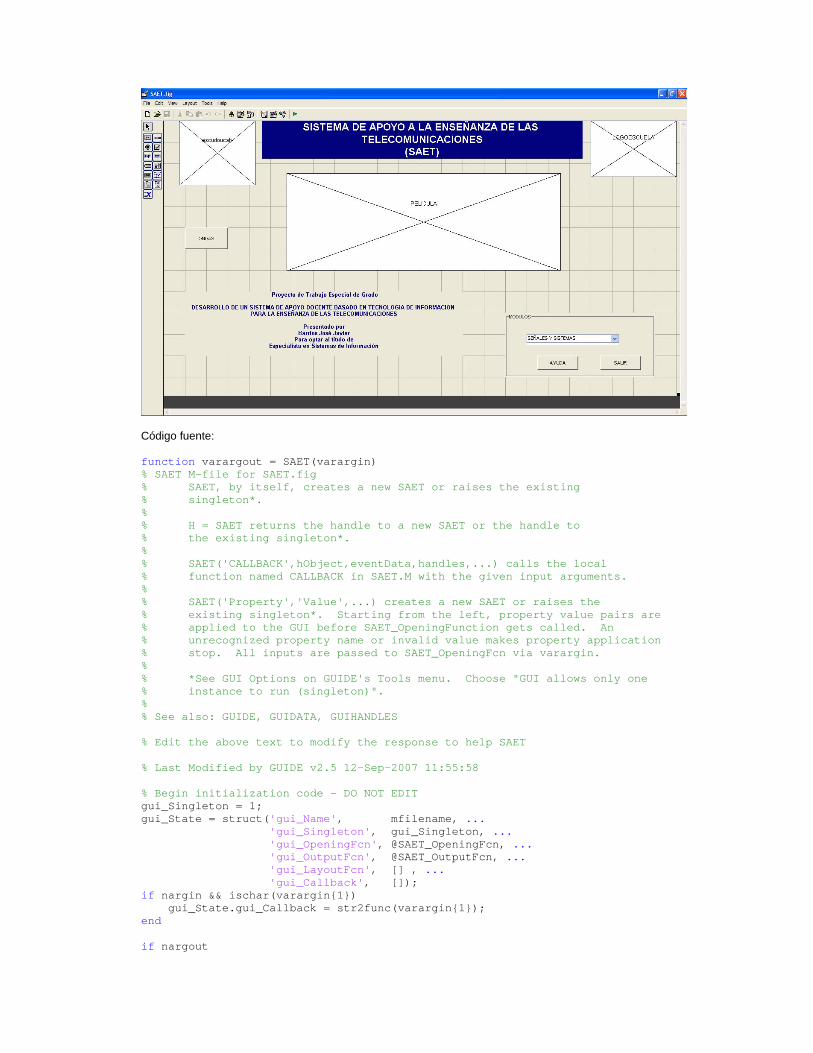
Código fuente: function varargout = SAET(varargin) % SAET M-file for SAET.fig % SAET, by itself, creates a new SAET or raises the existing % singleton*. % % H = SAET returns the handle to a new SAET or the handle to % the existing singleton*. % % SAET('CALLBACK',hObject,eventData,handles,...) calls the local % function named CALLBACK in SAET.M with the given input arguments. % % SAET('Property','Value',...) creates a new SAET or raises the % existing singleton*. Starting from the left, property value pairs are % applied to the GUI before SAET_OpeningFunction gets called. An % unrecognized property name or invalid value makes property application % stop. All inputs are passed to SAET_OpeningFcn via varargin. % % *See GUI Options on GUIDE's Tools menu. Choose "GUI allows only one % instance to run (singleton)". % % See also: GUIDE, GUIDATA, GUIHANDLES % Edit the above text to modify the response to help SAET % Last Modified by GUIDE v2.5 12-Sep-2007 11:55:58 % Begin initialization code - DO NOT EDIT gui_Singleton = 1; gui_State = struct('gui_Name', mfilename, ... 'gui_Singleton', gui_Singleton, ... 'gui_OpeningFcn', @SAET_OpeningFcn, ... 'gui_OutputFcn', @SAET_OutputFcn, ... 'gui_LayoutFcn', [] , ... 'gui_Callback', []); if nargin && ischar(varargin{1}) gui_State.gui_Callback = str2func(varargin{1}); end if nargout

[varargout{1:nargout}] = gui_mainfcn(gui_State, varargin{:}); else gui_mainfcn(gui_State, varargin{:}); end % End initialization code - DO NOT EDIT % --- Executes just before SAET is made visible. function SAET_OpeningFcn(hObject, eventdata, handles, varargin) % This function has no output args, see OutputFcn. % hObject handle to figure % eventdata reserved - to be defined in a future version of MATLAB % handles structure with handles and user data (see GUIDATA) % varargin command line arguments to SAET (see VARARGIN) % Choose default command line output for SAET %para el escudo ucab set(handles.escudoucab,'Visible','on'); axes(handles.escudoucab); image(imread('otro','jpeg')); set(handles.escudoucab,'Xtick',[]); set(handles.escudoucab,'Ytick',[]); %para el logo escuela set(handles.LOGOESCUELA,'Visible','on'); axes(handles.LOGOESCUELA); image(imread('otro2','jpeg')); set(handles.LOGOESCUELA,'Xtick',[]); set(handles.LOGOESCUELA,'Ytick',[]); handles.output = hObject; % Update handles structure guidata(hObject, handles); % UIWAIT makes SAET wait for user response (see UIRESUME) % uiwait(handles.figure1); % --- Outputs from this function are returned to the command line. function varargout = SAET_OutputFcn(hObject, eventdata, handles) % varargout cell array for returning output args (see VARARGOUT); % hObject handle to figure % eventdata reserved - to be defined in a future version of MATLAB % handles structure with handles and user data (see GUIDATA) % Get default command line output from handles structure varargout{1} = handles.output; % --- Executes on selection change in ESCOGER. function ESCOGER_Callback(hObject, eventdata, handles) % hObject handle to ESCOGER (see GCBO) % eventdata reserved - to be defined in a future version of MATLAB % handles structure with handles and user data (see GUIDATA) % Hints: contents = get(hObject,'String') returns ESCOGER contents as cell array % contents{get(hObject,'Value')} returns selected item from ESCOGER z=get(handles.ESCOGER,'value'); switch z case 1 SAETSENALES case 2 SAETCOMANALOGICAS case 3 SAETCOMDIGITALES otherwise,

end % --- Executes during object creation, after setting all properties. function ESCOGER_CreateFcn(hObject, eventdata, handles) % hObject handle to ESCOGER (see GCBO) % eventdata reserved - to be defined in a future version of MATLAB % handles empty - handles not created until after all CreateFcns called % Hint: popupmenu controls usually have a white background on Windows. % See ISPC and COMPUTER. if ispc && isequal(get(hObject,'BackgroundColor'), get(0,'defaultUicontrolBackgroundColor')) set(hObject,'BackgroundColor','white'); end % --- Executes on button press in VER. function VER_Callback(hObject, eventdata, handles) % hObject handle to VER (see GCBO) % eventdata reserved - to be defined in a future version of MATLAB % handles structure with handles and user data (see GUIDATA) ver=get(handles.VER,'value'); if ver==1, %pelicula M = moviein(50); x=[-2*pi:0.1:2*pi]; for j=1:50 y=sin(x+j*pi/8); y1=cos(x+j*pi/8); set(handles.PELICULA,'visible','off') axes(handles.PELICULA) plot(x,y,x,y1,'r'); M(:,j) = getframe; end u=-8:0.5:8; v=u; [U,V]=meshgrid(u,v); R=sqrt(U.^2+V.^2)+eps; W=sin(R)./R; surfc(W) end % --- Executes on button press in salir. function salir_Callback(hObject, eventdata, handles) % hObject handle to salir (see GCBO) % eventdata reserved - to be defined in a future version of MATLAB % handles structure with handles and user data (see GUIDATA) F=get(handles.salir,'value'); if F==1, salir end % --- Executes on button press in AYUDA. function AYUDA_Callback(hObject, eventdata, handles) % hObject handle to AYUDA (see GCBO) % eventdata reserved - to be defined in a future version of MATLAB % handles structure with handles and user data (see GUIDATA) F2=get(handles.AYUDA,'value'); if F2==1, helpdlg('ELIJA EL MODULO A ESTUDIAR','AYUDA'); end

Código fuente: function varargout = SAETSENALES(varargin) % SAETSENALES M-file for SAETSENALES.fig % SAETSENALES, by itself, creates a new SAETSENALES or raises the existing % singleton*. % % H = SAETSENALES returns the handle to a new SAETSENALES or the handle to % the existing singleton*. % % SAETSENALES('CALLBACK',hObject,eventData,handles,...) calls the local % function named CALLBACK in SAETSENALES.M with the given input arguments. % % SAETSENALES('Property','Value',...) creates a new SAETSENALES or raises the % existing singleton*. Starting from the left, property value pairs are % applied to the GUI before SAETSENALES_OpeningFunction gets called. An % unrecognized property name or invalid value makes property application % stop. All inputs are passed to SAETSENALES_OpeningFcn via varargin. % % *See GUI Options on GUIDE's Tools menu. Choose "GUI allows only one % instance to run (singleton)". % % See also: GUIDE, GUIDATA, GUIHANDLES % Edit the above text to modify the response to help SAETSENALES % Last Modified by GUIDE v2.5 18-Aug-2007 09:20:27 % Begin initialization code - DO NOT EDIT gui_Singleton = 1; gui_State = struct('gui_Name', mfilename, ... 'gui_Singleton', gui_Singleton, ... 'gui_OpeningFcn', @SAETSENALES_OpeningFcn, ...

'gui_OutputFcn', @SAETSENALES_OutputFcn, ... 'gui_LayoutFcn', [] , ... 'gui_Callback', []); if nargin && ischar(varargin{1}) gui_State.gui_Callback = str2func(varargin{1}); end if nargout [varargout{1:nargout}] = gui_mainfcn(gui_State, varargin{:}); else gui_mainfcn(gui_State, varargin{:}); end % End initialization code - DO NOT EDIT % --- Executes just before SAETSENALES is made visible. function SAETSENALES_OpeningFcn(hObject, eventdata, handles, varargin) % This function has no output args, see OutputFcn. % hObject handle to figure % eventdata reserved - to be defined in a future version of MATLAB % handles structure with handles and user data (see GUIDATA) % varargin command line arguments to SAETSENALES (see VARARGIN) set(handles.imagen,'Visible','on'); axes(handles.imagen); image(imread('telecom5','jpeg')); set(handles.imagen,'Xtick',[]); set(handles.imagen,'Ytick',[]); %ver set(handles.voz,'visible','off') set(handles.espectrovoz,'visible','off') set(handles.senales,'visible','off') set(handles.espectrosenales,'visible','off') % Choose default command line output for SAETSENALES handles.output = hObject; % Update handles structure guidata(hObject, handles); % UIWAIT makes SAETSENALES wait for user response (see UIRESUME) % uiwait(handles.figure1); % --- Outputs from this function are returned to the command line. function varargout = SAETSENALES_OutputFcn(hObject, eventdata, handles) % varargout cell array for returning output args (see VARARGOUT); % hObject handle to figure % eventdata reserved - to be defined in a future version of MATLAB % handles structure with handles and user data (see GUIDATA) % Get default command line output from handles structure varargout{1} = handles.output; % --- Executes on button press in vervoz. function vervoz_Callback(hObject, eventdata, handles) % hObject handle to vervoz (see GCBO) % eventdata reserved - to be defined in a future version of MATLAB % handles structure with handles and user data (see GUIDATA) v=get(handles.vervoz,'value'); if v==1, [men,fs]=wavread('delta.wav'); wavplay(men,fs)

set(handles.voz,'visible','off') axes(handles.voz) plot(men) grid title('SEÑAL DE VOZ') XLABEL('TIEMPO') YLABEL('AMPLITUD') y=abs(fftshift(fft(men))); y=y./length(men); w=linspace(-4000,4000,length(men)); set(handles.espectrovoz,'visible','off') axes(handles.espectrovoz) plot(w,y) grid title('ESPECTRO DE FRECUENCIA') XLABEL('FRECUENCIA') YLABEL('AMPLITUD') end % --- Executes on button press in versenales. function versenales_Callback(hObject, eventdata, handles) % hObject handle to versenales (see GCBO) % eventdata reserved - to be defined in a future version of MATLAB % handles structure with handles and user data (see GUIDATA) v2=get(handles.versenales,'value'); if v2==1, M = moviein(50); % t=[-2*pi:0.1:2*pi]; t=-1/8000:1/8000:2; noise=(1/10)*randn(1,length(t)); for j=1:50, x=sin(2*(pi/4)*10*(t+j)); x=x-2; senal=(x+noise); y1=SAWTOOTH(2*(pi/4)*10*(t+j)); y1=y1+2; y2=square(2*(pi/4)*10*(t+j),50); set(handles.senales,'visible','on') axes(handles.senales) plot(t,x+noise,t,y1,t,y2,'r'); grid AXIS([0 2 -3 3]) title('DOMINIO DEL TIEMPO') XLABEL('TIEMPO') YLABEL('AMPLITUD') M(:,j) = getframe; end y=abs(fftshift(fft(senal))); y=y./length(t); w=linspace(-4000,4000,length(senal)); set(handles.espectrosenales,'visible','on') axes(handles.espectrosenales) plot(w,y) grid title('ESPECTRO DE FRECUENCIA') XLABEL('FRECUENCIA') YLABEL('AMPLITUD') end

% --- Executes on button press in irgeneracion. function irgeneracion_Callback(hObject, eventdata, handles) % hObject handle to irgeneracion (see GCBO) % eventdata reserved - to be defined in a future version of MATLAB % handles structure with handles and user data (see GUIDATA) I=get(handles.irgeneracion,'value'); if I==1, GENERACION1 end % -------------------------------------------------------------------- function Untitled_1_Callback(hObject, eventdata, handles) % hObject handle to Untitled_1 (see GCBO) % eventdata reserved - to be defined in a future version of MATLAB % handles structure with handles and user data (see GUIDATA) % --- Executes on button press in regresar. function regresar_Callback(hObject, eventdata, handles) % hObject handle to regresar (see GCBO) % eventdata reserved - to be defined in a future version of MATLAB % handles structure with handles and user data (see GUIDATA) reg=get(handles.regresar,'value'); switch reg case 1 SAET otherwise, end
Código fuente: function varargout = GENERACION1(varargin) % GENERACION1 M-file for GENERACION1.fig % GENERACION1, by itself, creates a new GENERACION1 or raises the existing % singleton*. % % H = GENERACION1 returns the handle to a new GENERACION1 or the handle to

% the existing singleton*. % % GENERACION1('CALLBACK',hObject,eventData,handles,...) calls the local % function named CALLBACK in GENERACION1.M with the given input arguments. % % GENERACION1('Property','Value',...) creates a new GENERACION1 or raises the % existing singleton*. Starting from the left, property value pairs are % applied to the GUI before GENERACION1_OpeningFunction gets called. An % unrecognized property name or invalid value makes property application % stop. All inputs are passed to GENERACION1_OpeningFcn via varargin. % % *See GUI Options on GUIDE's Tools menu. Choose "GUI allows only one % instance to run (singleton)". % % See also: GUIDE, GUIDATA, GUIHANDLES % Edit the above text to modify the response to help GENERACION1 % Last Modified by GUIDE v2.5 27-Sep-2007 12:47:17 % Begin initialization code - DO NOT EDIT gui_Singleton = 1; gui_State = struct('gui_Name', mfilename, ... 'gui_Singleton', gui_Singleton, ... 'gui_OpeningFcn', @GENERACION1_OpeningFcn, ... 'gui_OutputFcn', @GENERACION1_OutputFcn, ... 'gui_LayoutFcn', [] , ... 'gui_Callback', []); if nargin && ischar(varargin{1}) gui_State.gui_Callback = str2func(varargin{1}); end if nargout [varargout{1:nargout}] = gui_mainfcn(gui_State, varargin{:}); else gui_mainfcn(gui_State, varargin{:}); end % End initialization code - DO NOT EDIT % --- Executes just before GENERACION1 is made visible. function GENERACION1_OpeningFcn(hObject, eventdata, handles, varargin) % This function has no output args, see OutputFcn. % hObject handle to figure % eventdata reserved - to be defined in a future version of MATLAB % handles structure with handles and user data (see GUIDATA) % varargin command line arguments to GENERACION1 (see VARARGIN) % Choose default command line output for GENERACION1 handles.output = hObject; % Update handles structure guidata(hObject, handles); % UIWAIT makes GENERACION1 wait for user response (see UIRESUME) % uiwait(handles.figure1); % --- Outputs from this function are returned to the command line. function varargout = GENERACION1_OutputFcn(hObject, eventdata, handles) % varargout cell array for returning output args (see VARARGOUT); % hObject handle to figure % eventdata reserved - to be defined in a future version of MATLAB % handles structure with handles and user data (see GUIDATA) % Get default command line output from handles structure

varargout{1} = handles.output; % --- Executes on selection change in FUNCION1. function FUNCION1_Callback(hObject, eventdata, handles) % hObject handle to FUNCION1 (see GCBO) % eventdata reserved - to be defined in a future version of MATLAB % handles structure with handles and user data (see GUIDATA) % Hints: contents = get(hObject,'String') returns FUNCION1 contents as cell array % contents{get(hObject,'Value')} returns selected item from FUNCION1 % --- Executes during object creation, after setting all properties. function FUNCION1_CreateFcn(hObject, eventdata, handles) % hObject handle to FUNCION1 (see GCBO) % eventdata reserved - to be defined in a future version of MATLAB % handles empty - handles not created until after all CreateFcns called % Hint: popupmenu controls usually have a white background on Windows. % See ISPC and COMPUTER. if ispc && isequal(get(hObject,'BackgroundColor'), get(0,'defaultUicontrolBackgroundColor')) set(hObject,'BackgroundColor','white'); end % --- Executes on selection change in FORMADEONDA1. function FORMADEONDA1_Callback(hObject, eventdata, handles) % hObject handle to FORMADEONDA1 (see GCBO) % eventdata reserved - to be defined in a future version of MATLAB % handles structure with handles and user data (see GUIDATA) % Hints: contents = get(hObject,'String') returns FORMADEONDA1 contents as cell array % contents{get(hObject,'Value')} returns selected item from FORMADEONDA1 % --- Executes during object creation, after setting all properties. function FORMADEONDA1_CreateFcn(hObject, eventdata, handles) % hObject handle to FORMADEONDA1 (see GCBO) % eventdata reserved - to be defined in a future version of MATLAB % handles empty - handles not created until after all CreateFcns called % Hint: popupmenu controls usually have a white background on Windows. % See ISPC and COMPUTER. if ispc && isequal(get(hObject,'BackgroundColor'), get(0,'defaultUicontrolBackgroundColor')) set(hObject,'BackgroundColor','white'); end function AMPLITUD1_Callback(hObject, eventdata, handles) % hObject handle to AMPLITUD1 (see GCBO) % eventdata reserved - to be defined in a future version of MATLAB % handles structure with handles and user data (see GUIDATA) % Hints: get(hObject,'String') returns contents of AMPLITUD1 as text % str2double(get(hObject,'String')) returns contents of AMPLITUD1 as a double % --- Executes during object creation, after setting all properties. function AMPLITUD1_CreateFcn(hObject, eventdata, handles) % hObject handle to AMPLITUD1 (see GCBO)

% eventdata reserved - to be defined in a future version of MATLAB % handles empty - handles not created until after all CreateFcns called % Hint: edit controls usually have a white background on Windows. % See ISPC and COMPUTER. if ispc && isequal(get(hObject,'BackgroundColor'), get(0,'defaultUicontrolBackgroundColor')) set(hObject,'BackgroundColor','white'); end % --- Executes on slider movement. function FRECUENCIA1_Callback(hObject, eventdata, handles) % hObject handle to FRECUENCIA1 (see GCBO) % eventdata reserved - to be defined in a future version of MATLAB % handles structure with handles and user data (see GUIDATA) % Hints: get(hObject,'Value') returns position of slider % get(hObject,'Min') and get(hObject,'Max') to determine range of slider % --- Executes during object creation, after setting all properties. function FRECUENCIA1_CreateFcn(hObject, eventdata, handles) % hObject handle to FRECUENCIA1 (see GCBO) % eventdata reserved - to be defined in a future version of MATLAB % handles empty - handles not created until after all CreateFcns called % Hint: slider controls usually have a light gray background. if isequal(get(hObject,'BackgroundColor'), get(0,'defaultUicontrolBackgroundColor')) set(hObject,'BackgroundColor',[.9 .9 .9]); end function FRECUENCIA11_Callback(hObject, eventdata, handles) % hObject handle to FRECUENCIA11 (see GCBO) % eventdata reserved - to be defined in a future version of MATLAB % handles structure with handles and user data (see GUIDATA) % Hints: get(hObject,'String') returns contents of FRECUENCIA11 as text % str2double(get(hObject,'String')) returns contents of FRECUENCIA11 as a double % --- Executes during object creation, after setting all properties. function FRECUENCIA11_CreateFcn(hObject, eventdata, handles) % hObject handle to FRECUENCIA11 (see GCBO) % eventdata reserved - to be defined in a future version of MATLAB % handles empty - handles not created until after all CreateFcns called % Hint: edit controls usually have a white background on Windows. % See ISPC and COMPUTER. if ispc && isequal(get(hObject,'BackgroundColor'), get(0,'defaultUicontrolBackgroundColor')) set(hObject,'BackgroundColor','white'); end function OFFSET1_Callback(hObject, eventdata, handles) % hObject handle to OFFSET1 (see GCBO) % eventdata reserved - to be defined in a future version of MATLAB % handles structure with handles and user data (see GUIDATA) % Hints: get(hObject,'String') returns contents of OFFSET1 as text
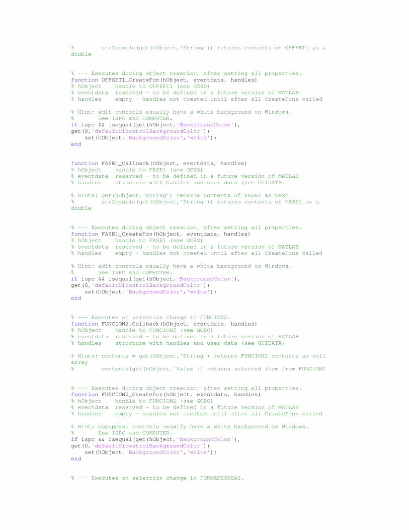
% str2double(get(hObject,'String')) returns contents of OFFSET1 as a double % --- Executes during object creation, after setting all properties. function OFFSET1_CreateFcn(hObject, eventdata, handles) % hObject handle to OFFSET1 (see GCBO) % eventdata reserved - to be defined in a future version of MATLAB % handles empty - handles not created until after all CreateFcns called % Hint: edit controls usually have a white background on Windows. % See ISPC and COMPUTER. if ispc && isequal(get(hObject,'BackgroundColor'), get(0,'defaultUicontrolBackgroundColor')) set(hObject,'BackgroundColor','white'); end function FASE1_Callback(hObject, eventdata, handles) % hObject handle to FASE1 (see GCBO) % eventdata reserved - to be defined in a future version of MATLAB % handles structure with handles and user data (see GUIDATA) % Hints: get(hObject,'String') returns contents of FASE1 as text % str2double(get(hObject,'String')) returns contents of FASE1 as a double % --- Executes during object creation, after setting all properties. function FASE1_CreateFcn(hObject, eventdata, handles) % hObject handle to FASE1 (see GCBO) % eventdata reserved - to be defined in a future version of MATLAB % handles empty - handles not created until after all CreateFcns called % Hint: edit controls usually have a white background on Windows. % See ISPC and COMPUTER. if ispc && isequal(get(hObject,'BackgroundColor'), get(0,'defaultUicontrolBackgroundColor')) set(hObject,'BackgroundColor','white'); end % --- Executes on selection change in FUNCION2. function FUNCION2_Callback(hObject, eventdata, handles) % hObject handle to FUNCION2 (see GCBO) % eventdata reserved - to be defined in a future version of MATLAB % handles structure with handles and user data (see GUIDATA) % Hints: contents = get(hObject,'String') returns FUNCION2 contents as cell array % contents{get(hObject,'Value')} returns selected item from FUNCION2 % --- Executes during object creation, after setting all properties. function FUNCION2_CreateFcn(hObject, eventdata, handles) % hObject handle to FUNCION2 (see GCBO) % eventdata reserved - to be defined in a future version of MATLAB % handles empty - handles not created until after all CreateFcns called % Hint: popupmenu controls usually have a white background on Windows. % See ISPC and COMPUTER. if ispc && isequal(get(hObject,'BackgroundColor'), get(0,'defaultUicontrolBackgroundColor')) set(hObject,'BackgroundColor','white'); end % --- Executes on selection change in FORMADEONDA2.

function FORMADEONDA2_Callback(hObject, eventdata, handles) % hObject handle to FORMADEONDA2 (see GCBO) % eventdata reserved - to be defined in a future version of MATLAB % handles structure with handles and user data (see GUIDATA) % Hints: contents = get(hObject,'String') returns FORMADEONDA2 contents as cell array % contents{get(hObject,'Value')} returns selected item from FORMADEONDA2 % --- Executes during object creation, after setting all properties. function FORMADEONDA2_CreateFcn(hObject, eventdata, handles) % hObject handle to FORMADEONDA2 (see GCBO) % eventdata reserved - to be defined in a future version of MATLAB % handles empty - handles not created until after all CreateFcns called % Hint: popupmenu controls usually have a white background on Windows. % See ISPC and COMPUTER. if ispc && isequal(get(hObject,'BackgroundColor'), get(0,'defaultUicontrolBackgroundColor')) set(hObject,'BackgroundColor','white'); end function AMPLITUD2_Callback(hObject, eventdata, handles) % hObject handle to AMPLITUD2 (see GCBO) % eventdata reserved - to be defined in a future version of MATLAB % handles structure with handles and user data (see GUIDATA) % Hints: get(hObject,'String') returns contents of AMPLITUD2 as text % str2double(get(hObject,'String')) returns contents of AMPLITUD2 as a double % --- Executes during object creation, after setting all properties. function AMPLITUD2_CreateFcn(hObject, eventdata, handles) % hObject handle to AMPLITUD2 (see GCBO) % eventdata reserved - to be defined in a future version of MATLAB % handles empty - handles not created until after all CreateFcns called % Hint: edit controls usually have a white background on Windows. % See ISPC and COMPUTER. if ispc && isequal(get(hObject,'BackgroundColor'), get(0,'defaultUicontrolBackgroundColor')) set(hObject,'BackgroundColor','white'); end % --- Executes on slider movement. function FRECUENCIA2_Callback(hObject, eventdata, handles) % hObject handle to FRECUENCIA2 (see GCBO) % eventdata reserved - to be defined in a future version of MATLAB % handles structure with handles and user data (see GUIDATA) % Hints: get(hObject,'Value') returns position of slider % get(hObject,'Min') and get(hObject,'Max') to determine range of slider % --- Executes during object creation, after setting all properties. function FRECUENCIA2_CreateFcn(hObject, eventdata, handles) % hObject handle to FRECUENCIA2 (see GCBO) % eventdata reserved - to be defined in a future version of MATLAB % handles empty - handles not created until after all CreateFcns called % Hint: slider controls usually have a light gray background.

if isequal(get(hObject,'BackgroundColor'), get(0,'defaultUicontrolBackgroundColor')) set(hObject,'BackgroundColor',[.9 .9 .9]); end function FRECUENCIA22_Callback(hObject, eventdata, handles) % hObject handle to FRECUENCIA22 (see GCBO) % eventdata reserved - to be defined in a future version of MATLAB % handles structure with handles and user data (see GUIDATA) % Hints: get(hObject,'String') returns contents of FRECUENCIA22 as text % str2double(get(hObject,'String')) returns contents of FRECUENCIA22 as a double % --- Executes during object creation, after setting all properties. function FRECUENCIA22_CreateFcn(hObject, eventdata, handles) % hObject handle to FRECUENCIA22 (see GCBO) % eventdata reserved - to be defined in a future version of MATLAB % handles empty - handles not created until after all CreateFcns called % Hint: edit controls usually have a white background on Windows. % See ISPC and COMPUTER. if ispc && isequal(get(hObject,'BackgroundColor'), get(0,'defaultUicontrolBackgroundColor')) set(hObject,'BackgroundColor','white'); end function OFFSET2_Callback(hObject, eventdata, handles) % hObject handle to OFFSET2 (see GCBO) % eventdata reserved - to be defined in a future version of MATLAB % handles structure with handles and user data (see GUIDATA) % Hints: get(hObject,'String') returns contents of OFFSET2 as text % str2double(get(hObject,'String')) returns contents of OFFSET2 as a double % --- Executes during object creation, after setting all properties. function OFFSET2_CreateFcn(hObject, eventdata, handles) % hObject handle to OFFSET2 (see GCBO) % eventdata reserved - to be defined in a future version of MATLAB % handles empty - handles not created until after all CreateFcns called % Hint: edit controls usually have a white background on Windows. % See ISPC and COMPUTER. if ispc && isequal(get(hObject,'BackgroundColor'), get(0,'defaultUicontrolBackgroundColor')) set(hObject,'BackgroundColor','white'); end function FASE2_Callback(hObject, eventdata, handles) % hObject handle to FASE2 (see GCBO) % eventdata reserved - to be defined in a future version of MATLAB % handles structure with handles and user data (see GUIDATA) % Hints: get(hObject,'String') returns contents of FASE2 as text % str2double(get(hObject,'String')) returns contents of FASE2 as a double % --- Executes during object creation, after setting all properties.

function FASE2_CreateFcn(hObject, eventdata, handles) % hObject handle to FASE2 (see GCBO) % eventdata reserved - to be defined in a future version of MATLAB % handles empty - handles not created until after all CreateFcns called % Hint: edit controls usually have a white background on Windows. % See ISPC and COMPUTER. if ispc && isequal(get(hObject,'BackgroundColor'), get(0,'defaultUicontrolBackgroundColor')) set(hObject,'BackgroundColor','white'); end % --- Executes on button press in PROCESAR1. function PROCESAR1_Callback(hObject, eventdata, handles) % hObject handle to PROCESAR1 (see GCBO) % eventdata reserved - to be defined in a future version of MATLAB % handles structure with handles and user data (see GUIDATA) A=get(handles.PROCESAR1,'value'); set(handles.AMPLITUD1,'visible','on') set(handles.AMPLITUD11,'visible','on') set(handles.FRECUENCIA1,'visible','on') set(handles.FRECUENCIA11,'visible','on') set(handles.FRECUENCIA111,'visible','on') set(handles.OFFSET1,'visible','on') set(handles.OFFSET11,'visible','on') set(handles.FASE1,'visible','on') set(handles.FASE11,'visible','on') if A==1, B=get(handles.FUNCION1,'value'); switch B case 1 %deterministica C=get(handles.FORMADEONDA1,'value'); set(handles.GRABAR1,'visible','off') switch C case 1 %onda seno global amplitud; global t; set(handles.CICLODETRABAJO1,'visible','off') set(handles.CICLODETRABAJO11,'visible','off') M = moviein(50); t=1/8000:1/8000:2; for j=1:50, amplitud=str2double(get(handles.AMPLITUD1,'String')); %validacion if isnan(amplitud) beep set(handles.AMPLITUD1,'String',0); amplitud=0; errordlg('El valor debe ser numérico','ERROR') end x=amplitud*sin(2*(pi/4)*10*(t+j)); set(handles.tiempo1,'visible','on') axes(handles.tiempo1) plot(t,x); grid AXIS([0 2 min(x) max(x)]) title('DOMINIO DEL TIEMPO') XLABEL('TIEMPO') YLABEL('AMPLITUD') M(:,j) = getframe; end cla global amplitud; global t; Fc=get(handles.FRECUENCIA1,'value'); Fc=Fc*1000; set(handles.FRECUENCIA11,'string',Fc)

offset=str2double(get(handles.OFFSET1,'String')); %validacion if isnan(offset) beep set(handles.OFFSET1,'String',0); offset=0; errordlg('El valor debe ser numérico','ERROR') end fase=str2double(get(handles.FASE1,'String')); %validacion if isnan(fase) beep set(handles.FASE1,'String',0); fase=0; errordlg('El valor debe ser numérico','ERROR') end %creo la forma de onda formadeonda1=amplitud*sin((2*pi*Fc*t)+fase); formadeonda1=formadeonda1+offset; save datos.mat formadeonda1 set(handles.tiempo1,'visible','on') axes(handles.tiempo1) plot(formadeonda1) grid AXIS([0 200 min(formadeonda1) max(formadeonda1)]) title('DOMINIO DEL TIEMPO') XLABEL('TIEMPO') YLABEL('AMPLITUD') %ESPECTRO EN FRECUENCIA y=abs(fftshift(fft(formadeonda1))); y=y./length(t); w=linspace(-4000,4000,length(formadeonda1)); set(handles.frecuencia1,'visible','on') axes(handles.frecuencia1) plot(w,y) grid title('ESPECTRO DE FRECUENCIA') XLABEL('FRECUENCIA') YLABEL('AMPLITUD') case 2 %onda coseno global amplitud; global t; set(handles.CICLODETRABAJO1,'visible','off') set(handles.CICLODETRABAJO11,'visible','off') M = moviein(50); t=1/8000:1/8000:2; for j=1:50, amplitud=str2double(get(handles.AMPLITUD1,'String')); %validacion if isnan(amplitud) beep set(handles.AMPLITUD1,'String',0); amplitud=0; errordlg('El valor debe ser numérico','ERROR') end x=amplitud*cos(2*(pi/4)*10*(t+j)); set(handles.tiempo1,'visible','on') axes(handles.tiempo1) plot(t,x,'r'); grid AXIS([0 2 min(x) max(x)]) title('DOMINIO DEL TIEMPO') XLABEL('TIEMPO') YLABEL('AMPLITUD') M(:,j) = getframe; end cla global amplitud;

global t; Fc=get(handles.FRECUENCIA1,'value'); Fc=Fc*1000; set(handles.FRECUENCIA11,'string',Fc) offset=str2double(get(handles.OFFSET1,'String')); %validacion if isnan(offset) beep set(handles.OFFSET1,'String',0); offset=0; errordlg('El valor debe ser numérico','ERROR') end fase=str2double(get(handles.FASE1,'String')); %validacion if isnan(fase) beep set(handles.FASE1,'String',0); fase=0; errordlg('El valor debe ser numérico','ERROR') end %creo la forma de onda formadeonda1=amplitud*cos((2*pi*Fc*t)+fase); formadeonda1=formadeonda1+offset; save datos.mat formadeonda1 set(handles.tiempo1,'visible','on') axes(handles.tiempo1) plot(formadeonda1,'r') grid AXIS([0 200 min(formadeonda1) max(formadeonda1)]) title('DOMINIO DEL TIEMPO') XLABEL('TIEMPO') YLABEL('AMPLITUD') %ESPECTRO EN FRECUENCIA y=abs(fftshift(fft(formadeonda1))); y=y./length(t); w=linspace(-4000,4000,length(formadeonda1)); set(handles.frecuencia1,'visible','on') axes(handles.frecuencia1) plot(w,y,'r') grid title('ESPECTRO DE FRECUENCIA') XLABEL('FRECUENCIA') YLABEL('AMPLITUD') case 3 %onda cuadrada global amplitud; global t; global ciclodetrabajo; set(handles.CICLODETRABAJO1,'visible','on') set(handles.CICLODETRABAJO11,'visible','on') M = moviein(50); t=1/8000:1/8000:2; for j=1:50, amplitud=str2double(get(handles.AMPLITUD1,'String')); if isnan(amplitud) beep set(handles.AMPLITUD1,'String',0); amplitud=0; errordlg('El valor debe ser numérico','ERROR') end ciclodetrabajo=str2double(get(handles.CICLODETRABAJO1,'String')); if isnan(ciclodetrabajo) beep set(handles.CICLODETRABAJO1,'String',50); ciclodetrabajo=50; errordlg('El valor debe ser numérico','ERROR') end if (ciclodetrabajo<=0) | (ciclodetrabajo>=100)

beep errordlg('El valor de ciclo de trabajo debe ser mayor que "0" y menor que "100" ','ERROR') set(handles.CICLODETRABAJO1,'String',50); ciclodetrabajo=50; end x=amplitud*square(2*(pi/4)*10*(t+j),ciclodetrabajo); set(handles.tiempo1,'visible','on') axes(handles.tiempo1) plot(t,x); grid AXIS([0 2 -50 50]) title('DOMINIO DEL TIEMPO') XLABEL('TIEMPO') YLABEL('AMPLITUD') M(:,j) = getframe; end cla global amplitud; global t; global ciclodetrabajo; Fc=get(handles.FRECUENCIA1,'value'); Fc=Fc*1000; set(handles.FRECUENCIA11,'string',Fc) offset=str2double(get(handles.OFFSET1,'String')); %validacion if isnan(offset) beep set(handles.OFFSET1,'String',0); offset=0; errordlg('El valor debe ser numérico','ERROR') end fase=str2double(get(handles.FASE1,'String')); %validacion if isnan(fase) beep set(handles.FASE1,'String',0); fase=0; errordlg('El valor debe ser numérico','ERROR') end %creo la forma de onda formadeonda1=amplitud*square((2*pi*Fc*t),ciclodetrabajo); formadeonda1=formadeonda1+offset; save datos.mat formadeonda1 set(handles.tiempo1,'visible','on') axes(handles.tiempo1) plot(formadeonda1) grid AXIS([0 200 -50 50]) title('DOMINIO DEL TIEMPO') XLABEL('TIEMPO') YLABEL('AMPLITUD') %ESPECTRO EN FRECUENCIA y=abs(fftshift(fft(formadeonda1))); y=y./length(t); w=linspace(-4000,4000,length(formadeonda1)); set(handles.frecuencia1,'visible','on') axes(handles.frecuencia1) plot(w,y) grid title('ESPECTRO DE FRECUENCIA') XLABEL('FRECUENCIA') YLABEL('AMPLITUD') case 4 %triangular global amplitud;
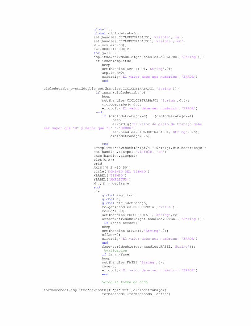
global t; global ciclodetrabajo; set(handles.CICLODETRABAJO1,'visible','on') set(handles.CICLODETRABAJO11,'visible','on') M = moviein(50); t=1/8000:1/8000:2; for j=1:50, amplitud=str2double(get(handles.AMPLITUD1,'String')); if isnan(amplitud) beep set(handles.AMPLITUD1,'String',0); amplitud=0; errordlg('El valor debe ser numérico','ERROR') end ciclodetrabajo=str2double(get(handles.CICLODETRABAJO1,'String')); if isnan(ciclodetrabajo) beep set(handles.CICLODETRABAJO1,'String',0.5); ciclodetrabajo=0.5; errordlg('El valor debe ser numérico','ERROR') end if (ciclodetrabajo<=0) | (ciclodetrabajo>=1) beep errordlg('El valor de ciclo de trabajo debe ser mayor que "0" y menor que "1" ','ERROR') set(handles.CICLODETRABAJO1,'String',0.5); ciclodetrabajo=0.5; end x=amplitud*sawtooth(2*(pi/4)*10*(t+j),ciclodetrabajo); set(handles.tiempo1,'visible','on') axes(handles.tiempo1) plot(t,x); grid AXIS([0 2 -50 50]) title('DOMINIO DEL TIEMPO') XLABEL('TIEMPO') YLABEL('AMPLITUD') M(:,j) = getframe; end cla global amplitud; global t; global ciclodetrabajo; Fc=get(handles.FRECUENCIA1,'value'); Fc=Fc*1000; set(handles.FRECUENCIA11,'string',Fc) offset=str2double(get(handles.OFFSET1,'String')); if isnan(offset) beep set(handles.OFFSET1,'String',0); offset=0; errordlg('El valor debe ser numérico','ERROR') end fase=str2double(get(handles.FASE1,'String')); %validacion if isnan(fase) beep set(handles.FASE1,'String',0); fase=0; errordlg('El valor debe ser numérico','ERROR') end %creo la forma de onda formadeonda1=amplitud*sawtooth((2*pi*Fc*t),ciclodetrabajo); formadeonda1=formadeonda1+offset;

save datos.mat formadeonda1 set(handles.tiempo1,'visible','on') axes(handles.tiempo1) plot(formadeonda1) grid AXIS([0 200 -50 50]) title('DOMINIO DEL TIEMPO') XLABEL('TIEMPO') YLABEL('AMPLITUD') %ESPECTRO EN FRECUENCIA y=abs(fftshift(fft(formadeonda1))); y=y./length(t); w=linspace(-4000,4000,length(formadeonda1)); set(handles.frecuencia1,'visible','on') axes(handles.frecuencia1) plot(w,y) grid title('ESPECTRO DE FRECUENCIA') XLABEL('FRECUENCIA') YLABEL('AMPLITUD') case 5 %diente de sierra global amplitud; global t; global ciclodetrabajo; M = moviein(50); t=1/8000:1/8000:2; for j=1:50, amplitud=str2double(get(handles.AMPLITUD1,'String')); if isnan(amplitud) beep set(handles.AMPLITUD1,'String',0); amplitud=0; errordlg('El valor debe ser numérico','ERROR') end x=amplitud*sawtooth(2*(pi/4)*10*(t+j),0.9); set(handles.tiempo1,'visible','on') axes(handles.tiempo1) plot(t,x); grid AXIS([0 2 -50 50]) title('DOMINIO DEL TIEMPO') XLABEL('TIEMPO') YLABEL('AMPLITUD') M(:,j) = getframe; end cla global amplitud; global t; global ciclodetrabajo; Fc=get(handles.FRECUENCIA1,'value'); Fc=Fc*1000; set(handles.FRECUENCIA11,'string',Fc) offset=str2double(get(handles.OFFSET1,'String')); if isnan(offset) beep set(handles.OFFSET1,'String',0); offset=0; errordlg('El valor debe ser numérico','ERROR') end fase=str2double(get(handles.FASE1,'String')); %validacion if isnan(fase) beep set(handles.FASE1,'String',0); fase=0; errordlg('El valor debe ser numérico','ERROR') end

%creo la forma de onda formadeonda1=amplitud*sawtooth((2*pi*Fc*t),0.9); formadeonda1=formadeonda1+offset; save datos.mat formadeonda1 set(handles.tiempo1,'visible','on') axes(handles.tiempo1) plot(formadeonda1) grid AXIS([0 200 -50 50]) title('DOMINIO DEL TIEMPO') XLABEL('TIEMPO') YLABEL('AMPLITUD') %ESPECTRO EN FRECUENCIA y=abs(fftshift(fft(formadeonda1))); y=y./length(t); w=linspace(-4000,4000,length(formadeonda1)); set(handles.frecuencia1,'visible','on') axes(handles.frecuencia1) plot(w,y) grid title('ESPECTRO DE FRECUENCIA') XLABEL('FRECUENCIA') YLABEL('AMPLITUD') case 6 %voz set(handles.GRABAR1,'visible','on') set(handles.AMPLITUD1,'visible','off') set(handles.AMPLITUD11,'visible','off') set(handles.FRECUENCIA1,'visible','off') set(handles.FRECUENCIA11,'visible','off') set(handles.FRECUENCIA111,'visible','off') set(handles.OFFSET1,'visible','off') set(handles.OFFSET11,'visible','off') set(handles.FASE1,'visible','off') set(handles.FASE11,'visible','off') set(handles.CICLODETRABAJO11,'visible','off') set(handles.CICLODETRABAJO1,'visible','off') %G=get(handles.GRABAR1,'value'); Fs = 11025*2; voz = wavrecord(16000, Fs); %cinco seg de grabacion formadeonda1=voz; global t; %formadeonda1=formadeonda1(1:16000); formadeonda1=formadeonda1'; save datos.mat formadeonda1 wavplay(voz, Fs); set(handles.tiempo1,'visible','on') axes(handles.tiempo1) grid plot(voz) title('DOMINIO TIEMPO') XLABEL('TIEMPO') YLABEL('AMPLITUD') %ESPECTRO EN FRECUENCIA y=abs(fftshift(fft(voz))); y=y./length(voz); w=linspace(-Fs/2,Fs/2,length(voz)); set(handles.frecuencia1,'visible','on') axes(handles.frecuencia1) plot(w,y) grid title('ESPECTRO DE FRECUENCIA') XLABEL('FRECUENCIA') YLABEL('AMPLITUD') case 7 %multitono seoidal

global amplitud; global t; set(handles.CICLODETRABAJO1,'visible','off') set(handles.CICLODETRABAJO11,'visible','off') M = moviein(50); t=1/8000:1/8000:2; for j=1:50, amplitud=str2double(get(handles.AMPLITUD1,'String')); if isnan(amplitud) beep set(handles.AMPLITUD1,'String',0); amplitud=0; errordlg('El valor debe ser numérico','ERROR') end x=amplitud*(0.75)*sin(2*(pi/4)*10*(t+j))+amplitud*(0.5)*sin(2*(pi/4)*15*(t+j))+amplitud*(0.25)*sin(2*(pi/4)*20*(t+j))+amplitud*(0.2)*sin(2*(pi/4)*5*(t+j)); set(handles.tiempo1,'visible','on') axes(handles.tiempo1) plot(t,x,'r'); grid AXIS([0 2 min(x) max(x)]) title('DOMINIO DEL TIEMPO') XLABEL('TIEMPO') YLABEL('AMPLITUD') M(:,j) = getframe; end cla global amplitud; global t; Fc=get(handles.FRECUENCIA1,'value'); Fc=Fc*1000; set(handles.FRECUENCIA11,'string',Fc) offset=str2double(get(handles.OFFSET1,'String')); if isnan(offset) beep set(handles.OFFSET1,'String',0); offset=0; errordlg('El valor debe ser numérico','ERROR') end fase=str2double(get(handles.FASE1,'String')); if isnan(fase) beep set(handles.FASE1,'String',0); fase=0; errordlg('El valor debe ser numérico','ERROR') end %creo la forma de onda formadeonda1=amplitud*(0.75)*sin(2*pi*1*Fc*t+fase)+(0.5)*amplitud*sin(2*pi*1.5*Fc*t+fase)+(0.25)*amplitud*sin(2*pi*2*Fc*t+fase)+(0.2)*amplitud*sin(2*pi*0.5*Fc*t+fase); formadeonda1=formadeonda1+offset; save datos.mat formadeonda1 set(handles.tiempo1,'visible','on') axes(handles.tiempo1) plot(formadeonda1,'r') grid AXIS([0 200 min(formadeonda1) max(formadeonda1)]) title('DOMINIO DEL TIEMPO') XLABEL('TIEMPO') YLABEL('AMPLITUD') %ESPECTRO EN FRECUENCIA y=abs(fftshift(fft(formadeonda1))); y=y./length(t); w=linspace(-4000,4000,length(formadeonda1)); set(handles.frecuencia1,'visible','on') axes(handles.frecuencia1)
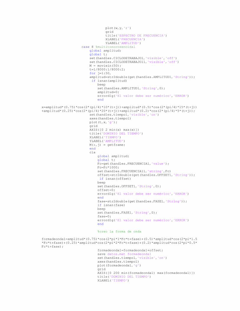
plot(w,y,'r') grid title('ESPECTRO DE FRECUENCIA') XLABEL('FRECUENCIA') YLABEL('AMPLITUD') case 8 %multitonocosenoidal global amplitud; global t; set(handles.CICLODETRABAJO1,'visible','off') set(handles.CICLODETRABAJO11,'visible','off') M = moviein(50); t=1/8000:1/8000:2; for j=1:50, amplitud=str2double(get(handles.AMPLITUD1,'String')); if isnan(amplitud) beep set(handles.AMPLITUD1,'String',0); amplitud=0; errordlg('El valor debe ser numérico','ERROR') end x=amplitud*(0.75)*cos(2*(pi/4)*10*(t+j))+amplitud*(0.5)*cos(2*(pi/4)*15*(t+j))+amplitud*(0.25)*cos(2*(pi/4)*20*(t+j))+amplitud*(0.2)*cos(2*(pi/4)*5*(t+j)); set(handles.tiempo1,'visible','on') axes(handles.tiempo1) plot(t,x,'g'); grid AXIS([0 2 min(x) max(x)]) title('DOMINIO DEL TIEMPO') XLABEL('TIEMPO') YLABEL('AMPLITUD') M(:,j) = getframe; end cla global amplitud; global t; Fc=get(handles.FRECUENCIA1,'value'); Fc=Fc*1000; set(handles.FRECUENCIA11,'string',Fc) offset=str2double(get(handles.OFFSET1,'String')); if isnan(offset) beep set(handles.OFFSET1,'String',0); offset=0; errordlg('El valor debe ser numérico','ERROR') end fase=str2double(get(handles.FASE1,'String')); if isnan(fase) beep set(handles.FASE1,'String',0); fase=0; errordlg('El valor debe ser numérico','ERROR') end %creo la forma de onda formadeonda1=amplitud*(0.75)*cos(2*pi*1*Fc*t+fase)+(0.5)*amplitud*cos(2*pi*1.5*Fc*t+fase)+(0.25)*amplitud*cos(2*pi*2*Fc*t+fase)+(0.2)*amplitud*cos(2*pi*0.5*Fc*t+fase); formadeonda1=formadeonda1+offset; save datos.mat formadeonda1 set(handles.tiempo1,'visible','on') axes(handles.tiempo1) plot(formadeonda1,'g') grid AXIS([0 200 min(formadeonda1) max(formadeonda1)]) title('DOMINIO DEL TIEMPO') XLABEL('TIEMPO')

YLABEL('AMPLITUD') %ESPECTRO EN FRECUENCIA y=abs(fftshift(fft(formadeonda1))); y=y./length(t); w=linspace(-4000,4000,length(formadeonda1)); set(handles.frecuencia1,'visible','on') axes(handles.frecuencia1) plot(w,y,'r') grid title('ESPECTRO DE FRECUENCIA') XLABEL('FRECUENCIA') YLABEL('AMPLITUD') otherwise, end case 2 %aleatoria (ruido) set(handles.FRECUENCIA1,'visible','off') set(handles.FRECUENCIA11,'visible','off') set(handles.FRECUENCIA111,'visible','off') set(handles.OFFSET1,'visible','off') set(handles.OFFSET11,'visible','off') set(handles.FASE1,'visible','off') set(handles.FASE11,'visible','off') set(handles.CICLODETRABAJO11,'visible','off') set(handles.CICLODETRABAJO1,'visible','off') M = moviein(50); t=1/8000:1/8000:2; for j=1:50, global amplitud; amplitud=str2double(get(handles.AMPLITUD1,'String')); if isnan(amplitud) beep set(handles.AMPLITUD1,'String',0); amplitud=0; errordlg('El valor debe ser numérico','ERROR') end x=(amplitud)*randn(1,length(t)); formadeonda1=x; save datos.mat formadeonda1 set(handles.tiempo1,'visible','on') axes(handles.tiempo1) plot(t,x); grid AXIS([0 0.2 -100 100]) title('DOMINIO DEL TIEMPO') XLABEL('TIEMPO') YLABEL('AMPLITUD') M(:,j) = getframe; end global amplitud; noise=amplitud*randn(1,length(t)); formadeonda1=noise; save datos.mat formadeonda1 set(handles.tiempo1,'visible','on') axes(handles.tiempo1) plot(t,noise,'r'); grid AXIS([0 0.2 -100 100]) title('DOMINIO DEL TIEMPO') XLABEL('TIEMPO') YLABEL('AMPLITUD') %ESPECTRO EN FRECUENCIA global t; y=abs(fftshift(fft(noise)));

y=y./length(t); w=linspace(-4000,4000,length(noise)); set(handles.frecuencia1,'visible','on') axes(handles.frecuencia1) plot(w,y) grid title('ESPECTRO DE FRECUENCIA') XLABEL('FRECUENCIA') YLABEL('AMPLITUD') otherwise, end end % --- Executes on button press in PROCESAR2. function PROCESAR2_Callback(hObject, eventdata, handles) % hObject handle to PROCESAR2 (see GCBO) % eventdata reserved - to be defined in a future version of MATLAB % handles structure with handles and user data (see GUIDATA) A=get(handles.PROCESAR2,'value'); set(handles.AMPLITUD2,'visible','on') set(handles.AMPLITUD22,'visible','on') set(handles.FRECUENCIA2,'visible','on') set(handles.FRECUENCIA22,'visible','on') set(handles.FRECUENCIA222,'visible','on') set(handles.OFFSET2,'visible','on') set(handles.OFFSET22,'visible','on') set(handles.FASE2,'visible','on') set(handles.FASE22,'visible','on') if A==1, B=get(handles.FUNCION2,'value'); switch B case 1 %deterministica C=get(handles.FORMADEONDA2,'value'); set(handles.GRABAR2,'visible','off') switch C case 1 %onda seno global amplitud; global t; set(handles.CICLODETRABAJO2,'visible','off') set(handles.CICLODETRABAJO22,'visible','off') M = moviein(50); t=1/8000:1/8000:2; for j=1:50, amplitud=str2double(get(handles.AMPLITUD2,'String')); if isnan(amplitud) beep set(handles.AMPLITUD2,'String',0); amplitud=0; errordlg('El valor debe ser numérico','ERROR') end x=amplitud*sin(2*(pi/4)*10*(t+j)); set(handles.tiempo2,'visible','on') axes(handles.tiempo2) plot(t,x); grid AXIS([0 2 min(x) max(x)]) title('DOMINIO DEL TIEMPO') XLABEL('TIEMPO') YLABEL('AMPLITUD') M(:,j) = getframe; end cla global amplitud; global t; Fc=get(handles.FRECUENCIA2,'value'); Fc=Fc*1000; set(handles.FRECUENCIA22,'string',Fc) offset=str2double(get(handles.OFFSET2,'String'));

if isnan(offset) beep set(handles.OFFSET2,'String',0); offset=0; errordlg('El valor debe ser numérico','ERROR') end fase=str2double(get(handles.FASE2,'String')); if isnan(fase) beep set(handles.FASE2,'String',0); fase=0; errordlg('El valor debe ser numérico','ERROR') end %creo la forma de onda formadeonda2=amplitud*sin((2*pi*Fc*t)+fase); formadeonda2=formadeonda2+offset; save datos1.mat formadeonda2 set(handles.tiempo2,'visible','on') axes(handles.tiempo2) plot(formadeonda2) grid AXIS([0 200 min(formadeonda2) max(formadeonda2)]) title('DOMINIO DEL TIEMPO') XLABEL('TIEMPO') YLABEL('AMPLITUD') %ESPECTRO EN FRECUENCIA y=abs(fftshift(fft(formadeonda2))); y=y./length(t); w=linspace(-4000,4000,length(formadeonda2)); set(handles.frecuencia2,'visible','on') axes(handles.frecuencia2) plot(w,y) grid title('ESPECTRO DE FRECUENCIA') XLABEL('FRECUENCIA') YLABEL('AMPLITUD') case 2 %onda coseno global amplitud; global t; set(handles.CICLODETRABAJO2,'visible','off') set(handles.CICLODETRABAJO22,'visible','off') M = moviein(50); t=1/8000:1/8000:2; for j=1:50, amplitud=str2double(get(handles.AMPLITUD2,'String')); if isnan(amplitud) beep set(handles.AMPLITUD2,'String',0); amplitud=0; errordlg('El valor debe ser numérico','ERROR') end x=amplitud*cos(2*(pi/4)*10*(t+j)); set(handles.tiempo2,'visible','on') axes(handles.tiempo2) plot(t,x,'r'); grid AXIS([0 2 min(x) max(x)]) title('DOMINIO DEL TIEMPO') XLABEL('TIEMPO') YLABEL('AMPLITUD') M(:,j) = getframe; end cla global amplitud; global t; Fc=get(handles.FRECUENCIA2,'value'); Fc=Fc*1000; set(handles.FRECUENCIA22,'string',Fc)

offset=str2double(get(handles.OFFSET2,'String')); if isnan(offset) beep set(handles.OFFSET2,'String',0); offset=0; errordlg('El valor debe ser numérico','ERROR') end fase=str2double(get(handles.FASE2,'String')); if isnan(fase) beep set(handles.FASE2,'String',0); fase=0; errordlg('El valor debe ser numérico','ERROR') end %creo la forma de onda formadeonda2=amplitud*sin((2*pi*Fc*t)+fase); formadeonda2=formadeonda2+offset; save datos1.mat formadeonda2 set(handles.tiempo2,'visible','on') axes(handles.tiempo2) plot(formadeonda2,'r') grid AXIS([0 200 min(formadeonda2) max(formadeonda2)]) title('DOMINIO DEL TIEMPO') XLABEL('TIEMPO') YLABEL('AMPLITUD') %ESPECTRO EN FRECUENCIA y=abs(fftshift(fft(formadeonda2))); y=y./length(t); w=linspace(-4000,4000,length(formadeonda2)); set(handles.frecuencia2,'visible','on') axes(handles.frecuencia2) plot(w,y,'r') grid title('ESPECTRO DE FRECUENCIA') XLABEL('FRECUENCIA') YLABEL('AMPLITUD') case 3 %onda cuadrada global amplitud; global t; global ciclodetrabajo; set(handles.CICLODETRABAJO2,'visible','on') set(handles.CICLODETRABAJO22,'visible','on') M = moviein(50); t=1/8000:1/8000:2; for j=1:50, amplitud=str2double(get(handles.AMPLITUD2,'String')); if isnan(amplitud) beep set(handles.AMPLITUD2,'String',0); amplitud=0; errordlg('El valor debe ser numérico','ERROR') end ciclodetrabajo=str2double(get(handles.CICLODETRABAJO2,'String')); if isnan(ciclodetrabajo) beep set(handles.CICLODETRABAJO2,'String',50); ciclodetrabajo=50; errordlg('El valor debe ser numérico','ERROR') end if (ciclodetrabajo<=0)|(ciclodetrabajo>=100) beep set(handles.CICLODETRABAJO2,'String',50); ciclodetrabajo=50; errordlg('El valor del ciclo de trabajo debe ser mayor que "0" y menor que "100%"','ERROR')

end x=amplitud*square(2*(pi/4)*10*(t+j),ciclodetrabajo); set(handles.tiempo2,'visible','on') axes(handles.tiempo2) plot(t,x); grid AXIS([0 2 -50 50]) title('DOMINIO DEL TIEMPO') XLABEL('TIEMPO') YLABEL('AMPLITUD') M(:,j) = getframe; end cla global amplitud; global t; global ciclodetrabajo; Fc=get(handles.FRECUENCIA2,'value'); Fc=Fc*1000; set(handles.FRECUENCIA22,'string',Fc) offset=str2double(get(handles.OFFSET2,'String')); if isnan(offset) beep set(handles.OFFSET2,'String',0); offset=0; errordlg('El valor debe ser numérico','ERROR') end fase=str2double(get(handles.FASE2,'String')); if isnan(fase) beep set(handles.FASE2,'String',0); fase=0; errordlg('El valor debe ser numérico','ERROR') end %creo la forma de onda formadeonda2=amplitud*square((2*pi*Fc*t),ciclodetrabajo); formadeonda2=formadeonda2+offset; save datos1.mat formadeonda2 set(handles.tiempo2,'visible','on') axes(handles.tiempo2) plot(formadeonda2) grid AXIS([0 200 -50 50]) title('DOMINIO DEL TIEMPO') XLABEL('TIEMPO') YLABEL('AMPLITUD') %ESPECTRO EN FRECUENCIA y=abs(fftshift(fft(formadeonda2))); y=y./length(t); w=linspace(-4000,4000,length(formadeonda2)); set(handles.frecuencia2,'visible','on') axes(handles.frecuencia2) plot(w,y) grid title('ESPECTRO DE FRECUENCIA') XLABEL('FRECUENCIA') YLABEL('AMPLITUD') case 4 %triangular global amplitud; global t; global ciclodetrabajo; set(handles.CICLODETRABAJO2,'visible','on') set(handles.CICLODETRABAJO22,'visible','on') M = moviein(50); t=1/8000:1/8000:2; for j=1:50, amplitud=str2double(get(handles.AMPLITUD2,'String'));

if isnan(amplitud) beep set(handles.AMPLITUD2,'String',0); amplitud=0; errordlg('El valor debe ser numérico','ERROR') end ciclodetrabajo=str2double(get(handles.CICLODETRABAJO2,'String')); if isnan(ciclodetrabajo) beep set(handles.CICLODETRABAJO2,'String',0.5); ciclodetrabajo=0.5; errordlg('El valor debe ser numérico','ERROR') end if (ciclodetrabajo<=0)|(ciclodetrabajo>=1) beep set(handles.CICLODETRABAJO2,'String',0.5); ciclodetrabajo=0.5; errordlg('El valor del ciclo de trabajo debe ser mayor que "0" y menor que "1"','ERROR') end x=amplitud*sawtooth(2*(pi/4)*10*(t+j),ciclodetrabajo); set(handles.tiempo2,'visible','on') axes(handles.tiempo2) plot(t,x); grid AXIS([0 2 -50 50]) title('DOMINIO DEL TIEMPO') XLABEL('TIEMPO') YLABEL('AMPLITUD') M(:,j) = getframe; end cla global amplitud; global t; global ciclodetrabajo; Fc=get(handles.FRECUENCIA2,'value'); Fc=Fc*1000; set(handles.FRECUENCIA22,'string',Fc) offset=str2double(get(handles.OFFSET2,'String')); if isnan(offset) beep set(handles.OFFSET2,'String',0); offset=0; errordlg('El valor debe ser numérico','ERROR') end fase=str2double(get(handles.FASE2,'String')); if isnan(fase) beep set(handles.FASE2,'String',0); fase=0; errordlg('El valor debe ser numérico','ERROR') end %creo la forma de onda formadeonda2=amplitud*sawtooth((2*pi*Fc*t),ciclodetrabajo); formadeonda2=formadeonda2+offset; save datos1.mat formadeonda2 set(handles.tiempo2,'visible','on') axes(handles.tiempo2) plot(formadeonda2) grid AXIS([0 200 -50 50]) title('DOMINIO DEL TIEMPO') XLABEL('TIEMPO') YLABEL('AMPLITUD')

%ESPECTRO EN FRECUENCIA y=abs(fftshift(fft(formadeonda2))); y=y./length(t); w=linspace(-4000,4000,length(formadeonda2)); set(handles.frecuencia2,'visible','on') axes(handles.frecuencia2) plot(w,y) grid title('ESPECTRO DE FRECUENCIA') XLABEL('FRECUENCIA') YLABEL('AMPLITUD') case 5 %diente de sierra global amplitud; global t; global ciclodetrabajo; M = moviein(50); t=1/8000:1/8000:2; for j=1:50, amplitud=str2double(get(handles.AMPLITUD2,'String')); if isnan(amplitud) beep set(handles.AMPLITUD2,'String',0); amplitud=0; errordlg('El valor debe ser numérico','ERROR') end x=amplitud*sawtooth(2*(pi/4)*10*(t+j),0.9); set(handles.tiempo2,'visible','on') axes(handles.tiempo2) plot(t,x); grid AXIS([0 2 -50 50]) title('DOMINIO DEL TIEMPO') XLABEL('TIEMPO') YLABEL('AMPLITUD') M(:,j) = getframe; end cla global amplitud; global t; global ciclodetrabajo; Fc=get(handles.FRECUENCIA2,'value'); Fc=Fc*1000; set(handles.FRECUENCIA22,'string',Fc) offset=str2double(get(handles.OFFSET2,'String')); if isnan(offset) beep set(handles.OFFSET2,'String',0); offset=0; errordlg('El valor debe ser numérico','ERROR') end fase=str2double(get(handles.FASE2,'String')); if isnan(fase) beep set(handles.FASE2,'String',0); fase=0; errordlg('El valor debe ser numérico','ERROR') end %creo la forma de onda formadeonda2=amplitud*sawtooth((2*pi*Fc*t),0.9); formadeonda2=formadeonda2+offset; save datos1.mat formadeonda2 set(handles.tiempo2,'visible','on') axes(handles.tiempo2) plot(formadeonda2) grid AXIS([0 200 -50 50])

title('DOMINIO DEL TIEMPO') XLABEL('TIEMPO') YLABEL('AMPLITUD') %ESPECTRO EN FRECUENCIA y=abs(fftshift(fft(formadeonda2))); y=y./length(t); w=linspace(-4000,4000,length(formadeonda2)); set(handles.frecuencia2,'visible','on') axes(handles.frecuencia2) plot(w,y) grid title('ESPECTRO DE FRECUENCIA') XLABEL('FRECUENCIA') YLABEL('AMPLITUD') case 6 %voz set(handles.GRABAR2,'visible','on') set(handles.AMPLITUD2,'visible','off') set(handles.AMPLITUD22,'visible','off') set(handles.FRECUENCIA2,'visible','off') set(handles.FRECUENCIA22,'visible','off') set(handles.FRECUENCIA222,'visible','off') set(handles.OFFSET2,'visible','off') set(handles.OFFSET22,'visible','off') set(handles.FASE2,'visible','off') set(handles.FASE22,'visible','off') set(handles.CICLODETRABAJO22,'visible','off') set(handles.CICLODETRABAJO2,'visible','off') %G=get(handles.GRABAR1,'value'); Fs = 11025*2; voz = wavrecord(16000, Fs); %cinco seg de grabacion formadeonda2=voz; global t; %formadeonda2=formadeonda2(1:16000); formadeonda2=formadeonda2'; save datos1.mat formadeonda2 wavplay(voz, Fs); set(handles.tiempo2,'visible','on') axes(handles.tiempo2) plot(voz) grid title('DOMINIO TIEMPO') XLABEL('TIEMPO') YLABEL('AMPLITUD') %ESPECTRO EN FRECUENCIA y=abs(fftshift(fft(voz))); y=y./length(voz); w=linspace(-Fs/2,Fs/2,length(voz)); set(handles.frecuencia2,'visible','on') axes(handles.frecuencia2) plot(w,y) grid title('ESPECTRO DE FRECUENCIA') XLABEL('FRECUENCIA') YLABEL('AMPLITUD') case 7 %multitono seoidal global amplitud; global t; set(handles.CICLODETRABAJO2,'visible','off') set(handles.CICLODETRABAJO22,'visible','off') M = moviein(50); t=1/8000:1/8000:2; for j=1:50, amplitud=str2double(get(handles.AMPLITUD2,'String')); if isnan(amplitud) beep
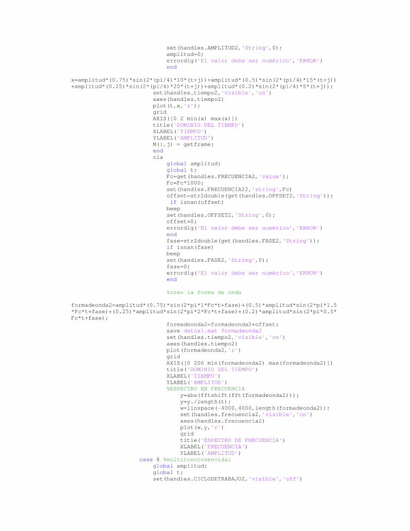
set(handles.AMPLITUD2,'String',0); amplitud=0; errordlg('El valor debe ser numérico','ERROR') end x=amplitud*(0.75)*sin(2*(pi/4)*10*(t+j))+amplitud*(0.5)*sin(2*(pi/4)*15*(t+j))+amplitud*(0.25)*sin(2*(pi/4)*20*(t+j))+amplitud*(0.2)*sin(2*(pi/4)*5*(t+j)); set(handles.tiempo2,'visible','on') axes(handles.tiempo2) plot(t,x,'r'); grid AXIS([0 2 min(x) max(x)]) title('DOMINIO DEL TIEMPO') XLABEL('TIEMPO') YLABEL('AMPLITUD') M(:,j) = getframe; end cla global amplitud; global t; Fc=get(handles.FRECUENCIA2,'value'); Fc=Fc*1000; set(handles.FRECUENCIA22,'string',Fc) offset=str2double(get(handles.OFFSET2,'String')); if isnan(offset) beep set(handles.OFFSET2,'String',0); offset=0; errordlg('El valor debe ser numérico','ERROR') end fase=str2double(get(handles.FASE2,'String')); if isnan(fase) beep set(handles.FASE2,'String',0); fase=0; errordlg('El valor debe ser numérico','ERROR') end %creo la forma de onda formadeonda2=amplitud*(0.75)*sin(2*pi*1*Fc*t+fase)+(0.5)*amplitud*sin(2*pi*1.5*Fc*t+fase)+(0.25)*amplitud*sin(2*pi*2*Fc*t+fase)+(0.2)*amplitud*sin(2*pi*0.5*Fc*t+fase); formadeonda2=formadeonda2+offset; save datos1.mat formadeonda2 set(handles.tiempo2,'visible','on') axes(handles.tiempo2) plot(formadeonda2,'r') grid AXIS([0 200 min(formadeonda2) max(formadeonda2)]) title('DOMINIO DEL TIEMPO') XLABEL('TIEMPO') YLABEL('AMPLITUD') %ESPECTRO EN FRECUENCIA y=abs(fftshift(fft(formadeonda2))); y=y./length(t); w=linspace(-4000,4000,length(formadeonda2)); set(handles.frecuencia2,'visible','on') axes(handles.frecuencia2) plot(w,y,'r') grid title('ESPECTRO DE FRECUENCIA') XLABEL('FRECUENCIA') YLABEL('AMPLITUD') case 8 %multitonocosenoidal global amplitud; global t; set(handles.CICLODETRABAJO2,'visible','off')

set(handles.CICLODETRABAJO22,'visible','off') M = moviein(50); t=1/8000:1/8000:2; for j=1:50, amplitud=str2double(get(handles.AMPLITUD2,'String')); if isnan(amplitud) beep set(handles.AMPLITUD2,'String',0); amplitud=0; errordlg('El valor debe ser numérico','ERROR') end x=amplitud*(0.75)*cos(2*(pi/4)*10*(t+j))+amplitud*(0.5)*cos(2*(pi/4)*15*(t+j))+amplitud*(0.25)*cos(2*(pi/4)*20*(t+j))+amplitud*(0.2)*cos(2*(pi/4)*5*(t+j)); set(handles.tiempo2,'visible','on') axes(handles.tiempo2) plot(t,x,'g'); grid AXIS([0 2 min(x) max(x)]) title('DOMINIO DEL TIEMPO') XLABEL('TIEMPO') YLABEL('AMPLITUD') M(:,j) = getframe; end cla global amplitud; global t; Fc=get(handles.FRECUENCIA2,'value'); Fc=Fc*1000; set(handles.FRECUENCIA22,'string',Fc) offset=str2double(get(handles.OFFSET2,'String')); if isnan(offset) beep set(handles.OFFSET2,'String',0); offset=0; errordlg('El valor debe ser numérico','ERROR') end fase=str2double(get(handles.FASE2,'String')); if isnan(fase) beep set(handles.FASE2,'String',0); fase=0; errordlg('El valor debe ser numérico','ERROR') end fase=str2double(get(handles.FASE2,'String')); %creo la forma de onda formadeonda2=amplitud*(0.75)*cos(2*pi*1*Fc*t+fase)+(0.5)*amplitud*cos(2*pi*1.5*Fc*t+fase)+(0.25)*amplitud*cos(2*pi*2*Fc*t+fase)+(0.2)*amplitud*cos(2*pi*0.5*Fc*t+fase); formadeonda2=formadeonda2+offset; save datos1.mat formadeonda2 set(handles.tiempo2,'visible','on') axes(handles.tiempo2) plot(formadeonda2,'g') grid AXIS([0 200 min(formadeonda2) max(formadeonda2)]) title('DOMINIO DEL TIEMPO') XLABEL('TIEMPO') YLABEL('AMPLITUD') %ESPECTRO EN FRECUENCIA y=abs(fftshift(fft(formadeonda2))); y=y./length(t); w=linspace(-4000,4000,length(formadeonda2)); set(handles.frecuencia2,'visible','on') axes(handles.frecuencia2) plot(w,y,'r') grid

title('ESPECTRO DE FRECUENCIA') XLABEL('FRECUENCIA') YLABEL('AMPLITUD') otherwise, end case 2 %aleatoria (ruido) set(handles.FRECUENCIA2,'visible','off') set(handles.FRECUENCIA22,'visible','off') set(handles.FRECUENCIA222,'visible','off') set(handles.OFFSET2,'visible','off') set(handles.OFFSET22,'visible','off') set(handles.FASE2,'visible','off') set(handles.FASE22,'visible','off') set(handles.CICLODETRABAJO22,'visible','off') set(handles.CICLODETRABAJO2,'visible','off') M = moviein(50); t=1/8000:1/8000:2; for j=1:50, global amplitud; amplitud=str2double(get(handles.AMPLITUD2,'String')); if isnan(amplitud) beep set(handles.AMPLITUD2,'String',0); amplitud=0; errordlg('El valor debe ser numérico','ERROR') end x=(amplitud)*randn(1,length(t)); set(handles.tiempo2,'visible','on') axes(handles.tiempo2) plot(t,x); grid AXIS([0 0.2 -100 100]) title('DOMINIO DEL TIEMPO') XLABEL('TIEMPO') YLABEL('AMPLITUD') M(:,j) = getframe; end global amplitud; noise=amplitud*randn(1,length(t)); formadeonda2=noise; save datos1.mat formadeonda2 set(handles.tiempo2,'visible','on') axes(handles.tiempo2) plot(t,noise,'r'); grid AXIS([0 0.2 -100 100]) title('DOMINIO DEL TIEMPO') XLABEL('TIEMPO') YLABEL('AMPLITUD') %ESPECTRO EN FRECUENCIA global t; y=abs(fftshift(fft(noise))); y=y./length(t); w=linspace(-4000,4000,length(noise)); set(handles.frecuencia2,'visible','on') axes(handles.frecuencia2) plot(w,y) grid title('ESPECTRO DE FRECUENCIA') XLABEL('FRECUENCIA') YLABEL('AMPLITUD') otherwise, end

end % --- Executes on button press in GRABAR1. function GRABAR1_Callback(hObject, eventdata, handles) % hObject handle to GRABAR1 (see GCBO) % eventdata reserved - to be defined in a future version of MATLAB % handles structure with handles and user data (see GUIDATA) % --- Executes on button press in GRABAR2. function GRABAR2_Callback(hObject, eventdata, handles) % hObject handle to GRABAR2 (see GCBO) % eventdata reserved - to be defined in a future version of MATLAB % handles structure with handles and user data (see GUIDATA) function CICLODETRABAJO1_Callback(hObject, eventdata, handles) % hObject handle to CICLODETRABAJO1 (see GCBO) % eventdata reserved - to be defined in a future version of MATLAB % handles structure with handles and user data (see GUIDATA) % Hints: get(hObject,'String') returns contents of CICLODETRABAJO1 as text % str2double(get(hObject,'String')) returns contents of CICLODETRABAJO1 as a double % --- Executes during object creation, after setting all properties. function CICLODETRABAJO1_CreateFcn(hObject, eventdata, handles) % hObject handle to CICLODETRABAJO1 (see GCBO) % eventdata reserved - to be defined in a future version of MATLAB % handles empty - handles not created until after all CreateFcns called % Hint: edit controls usually have a white background on Windows. % See ISPC and COMPUTER. if ispc && isequal(get(hObject,'BackgroundColor'), get(0,'defaultUicontrolBackgroundColor')) set(hObject,'BackgroundColor','white'); end function CICLODETRABAJO2_Callback(hObject, eventdata, handles) % hObject handle to CICLODETRABAJO2 (see GCBO) % eventdata reserved - to be defined in a future version of MATLAB % handles structure with handles and user data (see GUIDATA) % Hints: get(hObject,'String') returns contents of CICLODETRABAJO2 as text % str2double(get(hObject,'String')) returns contents of CICLODETRABAJO2 as a double % --- Executes during object creation, after setting all properties. function CICLODETRABAJO2_CreateFcn(hObject, eventdata, handles) % hObject handle to CICLODETRABAJO2 (see GCBO) % eventdata reserved - to be defined in a future version of MATLAB % handles empty - handles not created until after all CreateFcns called % Hint: edit controls usually have a white background on Windows. % See ISPC and COMPUTER. if ispc && isequal(get(hObject,'BackgroundColor'), get(0,'defaultUicontrolBackgroundColor')) set(hObject,'BackgroundColor','white'); end

% --- Executes on button press in regresar. function regresar_Callback(hObject, eventdata, handles) % hObject handle to regresar (see GCBO) % eventdata reserved - to be defined in a future version of MATLAB % handles structure with handles and user data (see GUIDATA) r=get(handles.regresar,'value'); if r==1, SAET end % --- Executes on button press in ALGEBRA. function ALGEBRA_Callback(hObject, eventdata, handles) % hObject handle to ALGEBRA (see GCBO) % eventdata reserved - to be defined in a future version of MATLAB % handles structure with handles and user data (see GUIDATA) r1=get(handles.ALGEBRA,'value'); if r1==1, ALGEBRAICA end % --- Executes on button press in IRFILTRAJE. function IRFILTRAJE_Callback(hObject, eventdata, handles) % hObject handle to IRFILTRAJE (see GCBO) % eventdata reserved - to be defined in a future version of MATLAB % handles structure with handles and user data (see GUIDATA) r11=get(handles.IRFILTRAJE,'value'); if r11==1, FILTRAJE end % --- Executes on button press in AYUDA. function AYUDA_Callback(hObject, eventdata, handles) % hObject handle to AYUDA (see GCBO) % eventdata reserved - to be defined in a future version of MATLAB % handles structure with handles and user data (see GUIDATA) r111=get(handles.AYUDA,'value'); if r111==1, open ('C:\Documents and Settings\javier\Mis documentos\TESIS_POSTGRADO\PARA LA TESIS\programas definitivos\ayudas\index_generacion.htm') end
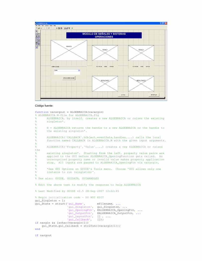
Código fuente: function varargout = ALGEBRAICA(varargin) % ALGEBRAICA M-file for ALGEBRAICA.fig % ALGEBRAICA, by itself, creates a new ALGEBRAICA or raises the existing % singleton*. % % H = ALGEBRAICA returns the handle to a new ALGEBRAICA or the handle to % the existing singleton*. % % ALGEBRAICA('CALLBACK',hObject,eventData,handles,...) calls the local % function named CALLBACK in ALGEBRAICA.M with the given input arguments. % % ALGEBRAICA('Property','Value',...) creates a new ALGEBRAICA or raises the % existing singleton*. Starting from the left, property value pairs are % applied to the GUI before ALGEBRAICA_OpeningFunction gets called. An % unrecognized property name or invalid value makes property application % stop. All inputs are passed to ALGEBRAICA_OpeningFcn via varargin. % % *See GUI Options on GUIDE's Tools menu. Choose "GUI allows only one % instance to run (singleton)". % % See also: GUIDE, GUIDATA, GUIHANDLES % Edit the above text to modify the response to help ALGEBRAICA % Last Modified by GUIDE v2.5 28-Sep-2007 12:22:45 % Begin initialization code - DO NOT EDIT gui_Singleton = 1; gui_State = struct('gui_Name', mfilename, ... 'gui_Singleton', gui_Singleton, ... 'gui_OpeningFcn', @ALGEBRAICA_OpeningFcn, ... 'gui_OutputFcn', @ALGEBRAICA_OutputFcn, ... 'gui_LayoutFcn', [] , ... 'gui_Callback', []); if nargin && ischar(varargin{1}) gui_State.gui_Callback = str2func(varargin{1}); end if nargout
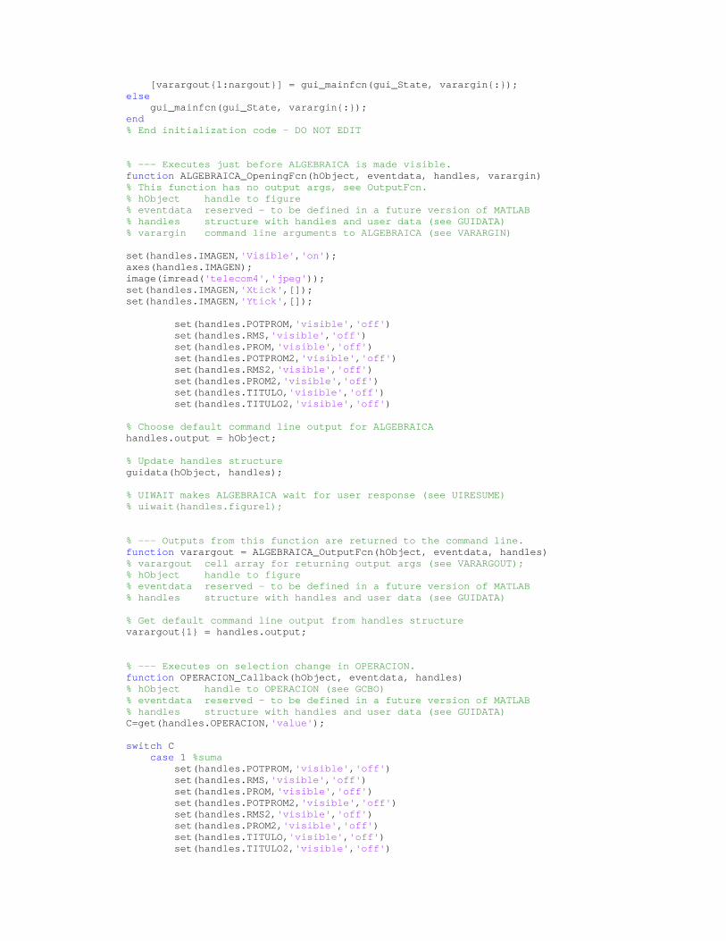
[varargout{1:nargout}] = gui_mainfcn(gui_State, varargin{:}); else gui_mainfcn(gui_State, varargin{:}); end % End initialization code - DO NOT EDIT % --- Executes just before ALGEBRAICA is made visible. function ALGEBRAICA_OpeningFcn(hObject, eventdata, handles, varargin) % This function has no output args, see OutputFcn. % hObject handle to figure % eventdata reserved - to be defined in a future version of MATLAB % handles structure with handles and user data (see GUIDATA) % varargin command line arguments to ALGEBRAICA (see VARARGIN) set(handles.IMAGEN,'Visible','on'); axes(handles.IMAGEN); image(imread('telecom4','jpeg')); set(handles.IMAGEN,'Xtick',[]); set(handles.IMAGEN,'Ytick',[]); set(handles.POTPROM,'visible','off') set(handles.RMS,'visible','off') set(handles.PROM,'visible','off') set(handles.POTPROM2,'visible','off') set(handles.RMS2,'visible','off') set(handles.PROM2,'visible','off') set(handles.TITULO,'visible','off') set(handles.TITULO2,'visible','off') % Choose default command line output for ALGEBRAICA handles.output = hObject; % Update handles structure guidata(hObject, handles); % UIWAIT makes ALGEBRAICA wait for user response (see UIRESUME) % uiwait(handles.figure1); % --- Outputs from this function are returned to the command line. function varargout = ALGEBRAICA_OutputFcn(hObject, eventdata, handles) % varargout cell array for returning output args (see VARARGOUT); % hObject handle to figure % eventdata reserved - to be defined in a future version of MATLAB % handles structure with handles and user data (see GUIDATA) % Get default command line output from handles structure varargout{1} = handles.output; % --- Executes on selection change in OPERACION. function OPERACION_Callback(hObject, eventdata, handles) % hObject handle to OPERACION (see GCBO) % eventdata reserved - to be defined in a future version of MATLAB % handles structure with handles and user data (see GUIDATA) C=get(handles.OPERACION,'value'); switch C case 1 %suma set(handles.POTPROM,'visible','off') set(handles.RMS,'visible','off') set(handles.PROM,'visible','off') set(handles.POTPROM2,'visible','off') set(handles.RMS2,'visible','off') set(handles.PROM2,'visible','off') set(handles.TITULO,'visible','off') set(handles.TITULO2,'visible','off')
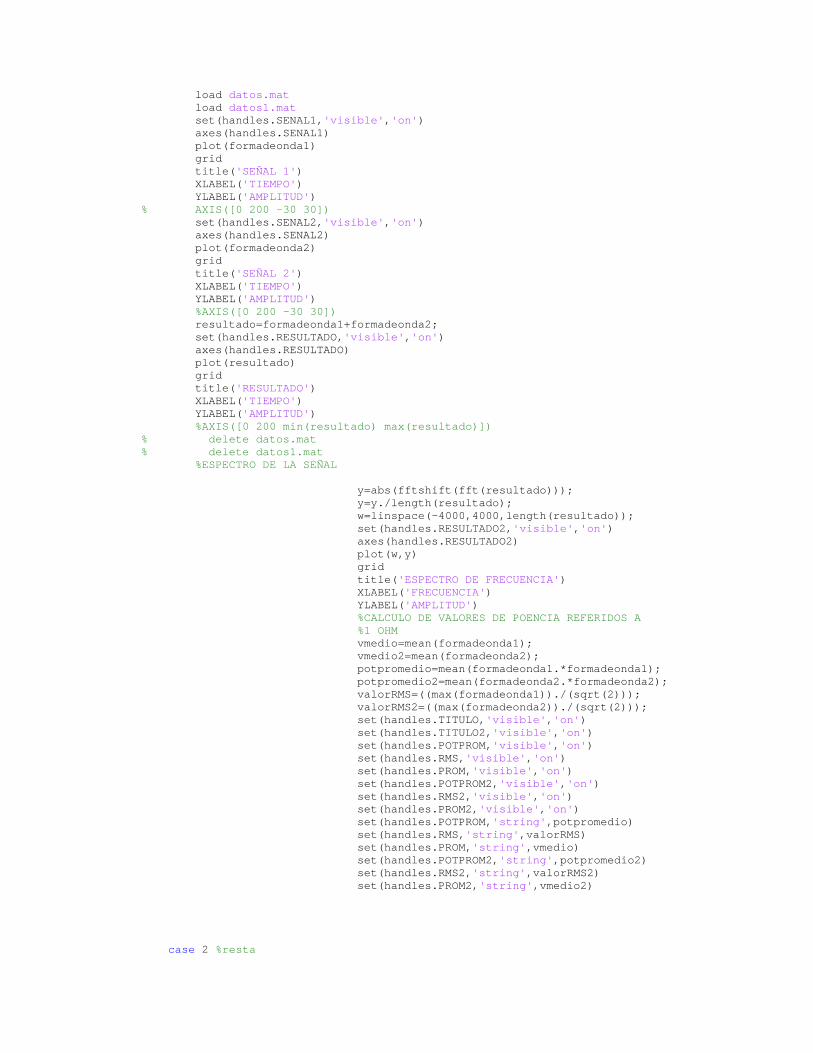
load datos.mat load datos1.mat set(handles.SENAL1,'visible','on') axes(handles.SENAL1) plot(formadeonda1) grid title('SEÑAL 1') XLABEL('TIEMPO') YLABEL('AMPLITUD') % AXIS([0 200 -30 30]) set(handles.SENAL2,'visible','on') axes(handles.SENAL2) plot(formadeonda2) grid title('SEÑAL 2') XLABEL('TIEMPO') YLABEL('AMPLITUD') %AXIS([0 200 -30 30]) resultado=formadeonda1+formadeonda2; set(handles.RESULTADO,'visible','on') axes(handles.RESULTADO) plot(resultado) grid title('RESULTADO') XLABEL('TIEMPO') YLABEL('AMPLITUD') %AXIS([0 200 min(resultado) max(resultado)]) % delete datos.mat % delete datos1.mat %ESPECTRO DE LA SEÑAL y=abs(fftshift(fft(resultado))); y=y./length(resultado); w=linspace(-4000,4000,length(resultado)); set(handles.RESULTADO2,'visible','on') axes(handles.RESULTADO2) plot(w,y) grid title('ESPECTRO DE FRECUENCIA') XLABEL('FRECUENCIA') YLABEL('AMPLITUD') %CALCULO DE VALORES DE POENCIA REFERIDOS A %1 OHM vmedio=mean(formadeonda1); vmedio2=mean(formadeonda2); potpromedio=mean(formadeonda1.*formadeonda1); potpromedio2=mean(formadeonda2.*formadeonda2); valorRMS=((max(formadeonda1))./(sqrt(2))); valorRMS2=((max(formadeonda2))./(sqrt(2))); set(handles.TITULO,'visible','on') set(handles.TITULO2,'visible','on') set(handles.POTPROM,'visible','on') set(handles.RMS,'visible','on') set(handles.PROM,'visible','on') set(handles.POTPROM2,'visible','on') set(handles.RMS2,'visible','on') set(handles.PROM2,'visible','on') set(handles.POTPROM,'string',potpromedio) set(handles.RMS,'string',valorRMS) set(handles.PROM,'string',vmedio) set(handles.POTPROM2,'string',potpromedio2) set(handles.RMS2,'string',valorRMS2) set(handles.PROM2,'string',vmedio2) case 2 %resta
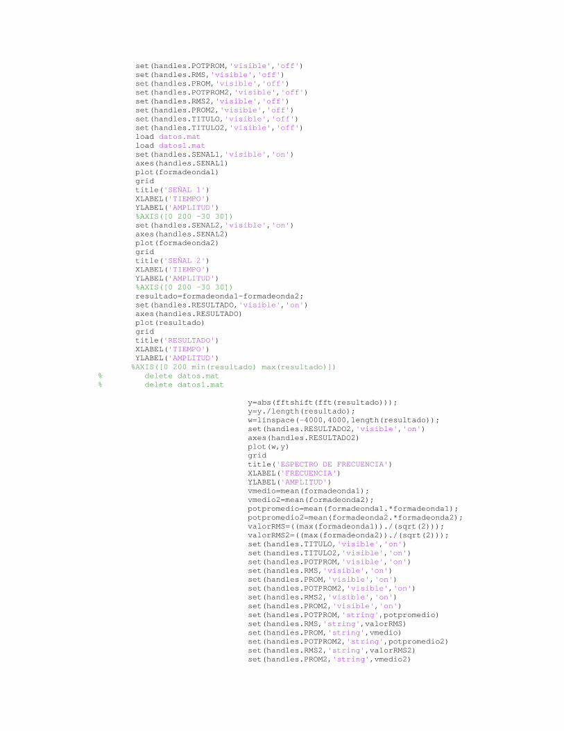
set(handles.POTPROM,'visible','off') set(handles.RMS,'visible','off') set(handles.PROM,'visible','off') set(handles.POTPROM2,'visible','off') set(handles.RMS2,'visible','off') set(handles.PROM2,'visible','off') set(handles.TITULO,'visible','off') set(handles.TITULO2,'visible','off') load datos.mat load datos1.mat set(handles.SENAL1,'visible','on') axes(handles.SENAL1) plot(formadeonda1) grid title('SEÑAL 1') XLABEL('TIEMPO') YLABEL('AMPLITUD') %AXIS([0 200 -30 30]) set(handles.SENAL2,'visible','on') axes(handles.SENAL2) plot(formadeonda2) grid title('SEÑAL 2') XLABEL('TIEMPO') YLABEL('AMPLITUD') %AXIS([0 200 -30 30]) resultado=formadeonda1-formadeonda2; set(handles.RESULTADO,'visible','on') axes(handles.RESULTADO) plot(resultado) grid title('RESULTADO') XLABEL('TIEMPO') YLABEL('AMPLITUD') %AXIS([0 200 min(resultado) max(resultado)]) % delete datos.mat % delete datos1.mat y=abs(fftshift(fft(resultado))); y=y./length(resultado); w=linspace(-4000,4000,length(resultado)); set(handles.RESULTADO2,'visible','on') axes(handles.RESULTADO2) plot(w,y) grid title('ESPECTRO DE FRECUENCIA') XLABEL('FRECUENCIA') YLABEL('AMPLITUD') vmedio=mean(formadeonda1); vmedio2=mean(formadeonda2); potpromedio=mean(formadeonda1.*formadeonda1); potpromedio2=mean(formadeonda2.*formadeonda2); valorRMS=((max(formadeonda1))./(sqrt(2))); valorRMS2=((max(formadeonda2))./(sqrt(2))); set(handles.TITULO,'visible','on') set(handles.TITULO2,'visible','on') set(handles.POTPROM,'visible','on') set(handles.RMS,'visible','on') set(handles.PROM,'visible','on') set(handles.POTPROM2,'visible','on') set(handles.RMS2,'visible','on') set(handles.PROM2,'visible','on') set(handles.POTPROM,'string',potpromedio) set(handles.RMS,'string',valorRMS) set(handles.PROM,'string',vmedio) set(handles.POTPROM2,'string',potpromedio2) set(handles.RMS2,'string',valorRMS2) set(handles.PROM2,'string',vmedio2)

case 3 %multiplicacion set(handles.POTPROM,'visible','off') set(handles.RMS,'visible','off') set(handles.PROM,'visible','off') set(handles.POTPROM2,'visible','off') set(handles.RMS2,'visible','off') set(handles.PROM2,'visible','off') set(handles.TITULO,'visible','off') set(handles.TITULO2,'visible','off') load datos.mat load datos1.mat set(handles.SENAL1,'visible','on') axes(handles.SENAL1) plot(formadeonda1) grid title('SEÑAL 1') XLABEL('TIEMPO') YLABEL('AMPLITUD') %AXIS([0 200 -30 30]) set(handles.SENAL2,'visible','on') axes(handles.SENAL2) plot(formadeonda2) grid title('SEÑAL 2') XLABEL('TIEMPO') YLABEL('AMPLITUD') %AXIS([0 200 -30 30]) resultado=formadeonda1.*formadeonda2; set(handles.RESULTADO,'visible','on') axes(handles.RESULTADO) plot(resultado) grid title('RESULTADO') XLABEL('TIEMPO') YLABEL('AMPLITUD') %AXIS([0 200 min(resultado) max(resultado)]) % delete datos.mat % delete datos1.mat y=abs(fftshift(fft(resultado))); y=y./length(resultado); w=linspace(-4000,4000,length(resultado)); set(handles.RESULTADO2,'visible','on') axes(handles.RESULTADO2) plot(w,y) grid title('ESPECTRO DE FRECUENCIA') XLABEL('FRECUENCIA') YLABEL('AMPLITUD') vmedio=mean(formadeonda1); vmedio2=mean(formadeonda2); potpromedio=mean(formadeonda1.*formadeonda1); potpromedio2=mean(formadeonda2.*formadeonda2); valorRMS=((max(formadeonda1))./(sqrt(2))); valorRMS2=((max(formadeonda2))./(sqrt(2))); set(handles.TITULO,'visible','on') set(handles.TITULO2,'visible','on') set(handles.POTPROM,'visible','on') set(handles.RMS,'visible','on') set(handles.PROM,'visible','on') set(handles.POTPROM2,'visible','on') set(handles.RMS2,'visible','on') set(handles.PROM2,'visible','on') set(handles.POTPROM,'string',potpromedio) set(handles.RMS,'string',valorRMS) set(handles.PROM,'string',vmedio) set(handles.POTPROM2,'string',potpromedio2) set(handles.RMS2,'string',valorRMS2)

set(handles.PROM2,'string',vmedio2) case 4 %dividir set(handles.POTPROM,'visible','off') set(handles.RMS,'visible','off') set(handles.PROM,'visible','off') set(handles.POTPROM2,'visible','off') set(handles.RMS2,'visible','off') set(handles.PROM2,'visible','off') set(handles.TITULO,'visible','off') set(handles.TITULO2,'visible','off') load datos.mat load datos1.mat set(handles.SENAL1,'visible','on') axes(handles.SENAL1) plot(formadeonda1) grid title('SEÑAL 1') XLABEL('TIEMPO') YLABEL('AMPLITUD') % AXIS([0 200 -30 30]) set(handles.SENAL2,'visible','on') axes(handles.SENAL2) plot(formadeonda2) grid title('SEÑAL 2') XLABEL('TIEMPO') YLABEL('AMPLITUD') %AXIS([0 200 -30 30]) resultado=formadeonda1./formadeonda2; set(handles.RESULTADO,'visible','on') axes(handles.RESULTADO) plot(resultado) grid title('RESULTADO') XLABEL('TIEMPO') YLABEL('AMPLITUD') %AXIS([0 200 min(resultado) max(resultado)]) % delete datos.mat % delete datos1.mat %ESPECTRO DE LA SEÑAL y=abs(fftshift(fft(resultado))); y=y./length(resultado); w=linspace(-4000,4000,length(resultado)); set(handles.RESULTADO2,'visible','on') axes(handles.RESULTADO2) plot(w,y) grid title('ESPECTRO DE FRECUENCIA') XLABEL('FRECUENCIA') YLABEL('AMPLITUD') vmedio=mean(formadeonda1); vmedio2=mean(formadeonda2); potpromedio=mean(formadeonda1.*formadeonda1); potpromedio2=mean(formadeonda2.*formadeonda2); valorRMS=((max(formadeonda1))./(sqrt(2))); valorRMS2=((max(formadeonda2))./(sqrt(2))); set(handles.TITULO,'visible','on') set(handles.TITULO2,'visible','on') set(handles.POTPROM,'visible','on') set(handles.RMS,'visible','on') set(handles.PROM,'visible','on') set(handles.POTPROM2,'visible','on') set(handles.RMS2,'visible','on') set(handles.PROM2,'visible','on') set(handles.POTPROM,'string',potpromedio) set(handles.RMS,'string',valorRMS) set(handles.PROM,'string',vmedio)

set(handles.POTPROM2,'string',potpromedio2) set(handles.RMS2,'string',valorRMS2) set(handles.PROM2,'string',vmedio2) case 5 %normalizar set(handles.POTPROM,'visible','off') set(handles.RMS,'visible','off') set(handles.PROM,'visible','off') set(handles.POTPROM2,'visible','off') set(handles.RMS2,'visible','off') set(handles.PROM2,'visible','off') set(handles.TITULO,'visible','off') set(handles.TITULO2,'visible','off') load datos.mat load datos1.mat set(handles.SENAL1,'visible','on') axes(handles.SENAL1) formadeonda1=formadeonda1./abs(min(formadeonda1)); plot(formadeonda1) grid title('SEÑAL 1') XLABEL('TIEMPO') YLABEL('AMPLITUD') % AXIS([0 200 -30 30]) set(handles.SENAL2,'visible','on') axes(handles.SENAL2) formadeonda2=formadeonda2./abs(min(formadeonda2)); plot(formadeonda2) grid title('SEÑAL 2') XLABEL('TIEMPO') YLABEL('AMPLITUD') %AXIS([0 200 -30 30]) y=abs(fftshift(fft(formadeonda1))); y=y./length(formadeonda1); w=linspace(-4000,4000,length(formadeonda1)); set(handles.RESULTADO,'visible','on') axes(handles.RESULTADO) plot(w,y) grid title('ESPECTRO DE FRECUENCIA') XLABEL('FRECUENCIA') YLABEL('AMPLITUD') vmedio=mean(formadeonda1); vmedio2=mean(formadeonda2); potpromedio=mean(formadeonda1.*formadeonda1); potpromedio2=mean(formadeonda2.*formadeonda2); valorRMS=((max(formadeonda1))./(sqrt(2))); valorRMS2=((max(formadeonda2))./(sqrt(2))); set(handles.TITULO,'visible','on') set(handles.TITULO2,'visible','on') set(handles.POTPROM,'visible','on') set(handles.RMS,'visible','on') set(handles.PROM,'visible','on') set(handles.POTPROM2,'visible','on') set(handles.RMS2,'visible','on') set(handles.PROM2,'visible','on') set(handles.POTPROM,'string',potpromedio) set(handles.RMS,'string',valorRMS) set(handles.PROM,'string',vmedio) set(handles.POTPROM2,'string',potpromedio2) set(handles.RMS2,'string',valorRMS2) set(handles.PROM2,'string',vmedio2) %AXIS([0 200 min(resultado) max(resultado)]) % delete datos.mat % delete datos1.mat %ESPECTRO DE LA SEÑAL
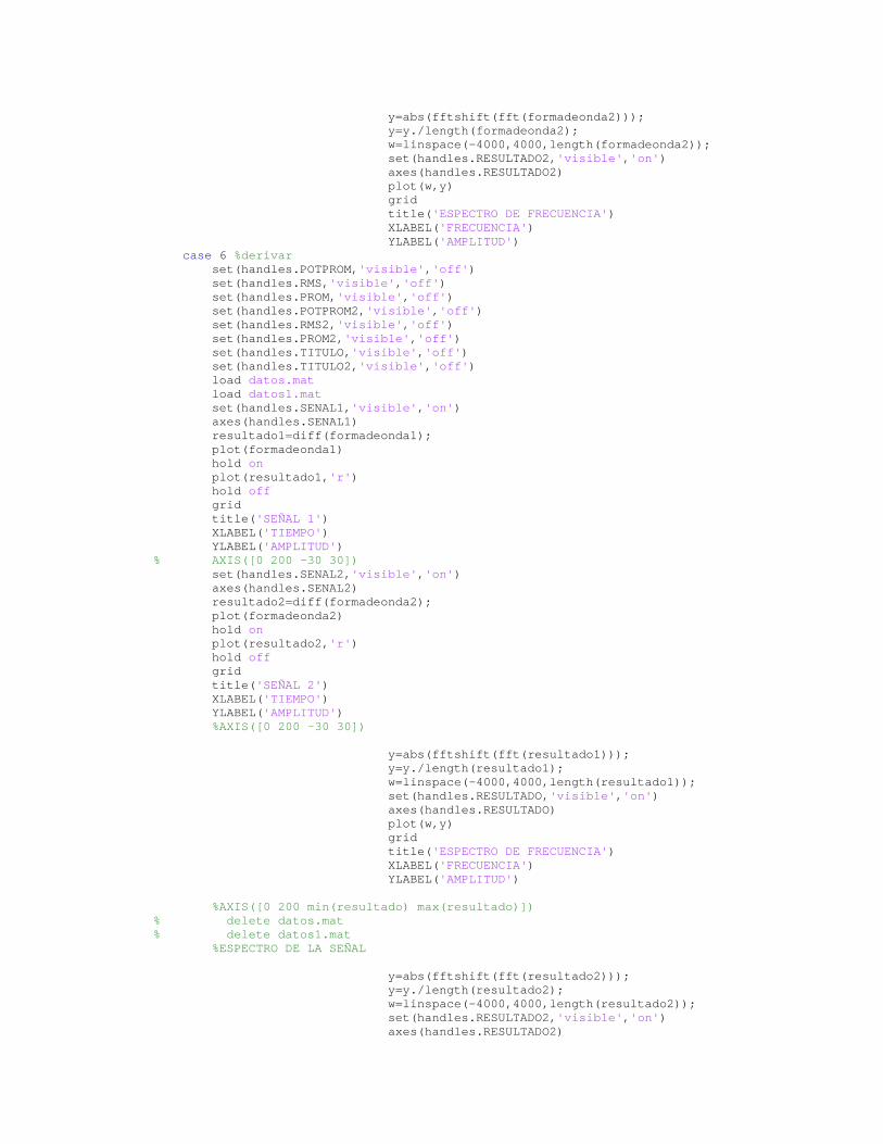
y=abs(fftshift(fft(formadeonda2))); y=y./length(formadeonda2); w=linspace(-4000,4000,length(formadeonda2)); set(handles.RESULTADO2,'visible','on') axes(handles.RESULTADO2) plot(w,y) grid title('ESPECTRO DE FRECUENCIA') XLABEL('FRECUENCIA') YLABEL('AMPLITUD') case 6 %derivar set(handles.POTPROM,'visible','off') set(handles.RMS,'visible','off') set(handles.PROM,'visible','off') set(handles.POTPROM2,'visible','off') set(handles.RMS2,'visible','off') set(handles.PROM2,'visible','off') set(handles.TITULO,'visible','off') set(handles.TITULO2,'visible','off') load datos.mat load datos1.mat set(handles.SENAL1,'visible','on') axes(handles.SENAL1) resultado1=diff(formadeonda1); plot(formadeonda1) hold on plot(resultado1,'r') hold off grid title('SEÑAL 1') XLABEL('TIEMPO') YLABEL('AMPLITUD') % AXIS([0 200 -30 30]) set(handles.SENAL2,'visible','on') axes(handles.SENAL2) resultado2=diff(formadeonda2); plot(formadeonda2) hold on plot(resultado2,'r') hold off grid title('SEÑAL 2') XLABEL('TIEMPO') YLABEL('AMPLITUD') %AXIS([0 200 -30 30]) y=abs(fftshift(fft(resultado1))); y=y./length(resultado1); w=linspace(-4000,4000,length(resultado1)); set(handles.RESULTADO,'visible','on') axes(handles.RESULTADO) plot(w,y) grid title('ESPECTRO DE FRECUENCIA') XLABEL('FRECUENCIA') YLABEL('AMPLITUD') %AXIS([0 200 min(resultado) max(resultado)]) % delete datos.mat % delete datos1.mat %ESPECTRO DE LA SEÑAL y=abs(fftshift(fft(resultado2))); y=y./length(resultado2); w=linspace(-4000,4000,length(resultado2)); set(handles.RESULTADO2,'visible','on') axes(handles.RESULTADO2)

plot(w,y) grid title('ESPECTRO DE FRECUENCIA') XLABEL('FRECUENCIA') YLABEL('AMPLITUD') vmedio=mean(formadeonda1); vmedio2=mean(formadeonda2); potpromedio=mean(formadeonda1.*formadeonda1); potpromedio2=mean(formadeonda2.*formadeonda2); valorRMS=((max(formadeonda1))./(sqrt(2))); valorRMS2=((max(formadeonda2))./(sqrt(2))); set(handles.TITULO,'visible','on') set(handles.TITULO2,'visible','on') set(handles.POTPROM,'visible','on') set(handles.RMS,'visible','on') set(handles.PROM,'visible','on') set(handles.POTPROM2,'visible','on') set(handles.RMS2,'visible','on') set(handles.PROM2,'visible','on') set(handles.POTPROM,'string',potpromedio) set(handles.RMS,'string',valorRMS) set(handles.PROM,'string',vmedio) set(handles.POTPROM2,'string',potpromedio2) set(handles.RMS2,'string',valorRMS2) set(handles.PROM2,'string',vmedio2) case 7 %DEP set(handles.POTPROM,'visible','off') set(handles.RMS,'visible','off') set(handles.PROM,'visible','off') set(handles.POTPROM2,'visible','off') set(handles.RMS2,'visible','off') set(handles.PROM2,'visible','off') set(handles.TITULO,'visible','off') set(handles.TITULO2,'visible','off') load datos.mat load datos1.mat set(handles.SENAL1,'visible','on') axes(handles.SENAL1) plot(formadeonda1) grid title('SEÑAL 1') XLABEL('TIEMPO') YLABEL('AMPLITUD') % AXIS([0 200 -30 30]) set(handles.SENAL2,'visible','on') axes(handles.SENAL2) plot(formadeonda2) grid title('SEÑAL 2') XLABEL('TIEMPO') YLABEL('AMPLITUD') %AXIS([0 200 -30 30]) %DEP de la señal c=xcorr(formadeonda1,formadeonda1); y=abs(fftshift(fft(c))); y=y./length(formadeonda1); w=linspace(-4000,4000,length(c)); set(handles.RESULTADO,'visible','on') axes(handles.RESULTADO) plot(w,y) grid title('DEP DE LA SEÑAL') XLABEL('FRECUENCIA') YLABEL('AMPLITUD')

%DEP de la señal2 c2=xcorr(formadeonda2,formadeonda2); y2=abs(fftshift(fft(c2))); y2=y2./length(formadeonda2); w=linspace(-4000,4000,length(c2)); set(handles.RESULTADO2,'visible','on') axes(handles.RESULTADO2) plot(w,y2) grid title('DEP DE LA SEÑAL') XLABEL('FRECUENCIA') YLABEL('AMPLITUD') vmedio=mean(formadeonda1); vmedio2=mean(formadeonda2); potpromedio=mean(formadeonda1.*formadeonda1); potpromedio2=mean(formadeonda2.*formadeonda2); valorRMS=((max(formadeonda1))./(sqrt(2))); valorRMS2=((max(formadeonda2))./(sqrt(2))); set(handles.TITULO,'visible','on') set(handles.TITULO2,'visible','on') set(handles.POTPROM,'visible','on') set(handles.RMS,'visible','on') set(handles.PROM,'visible','on') set(handles.POTPROM2,'visible','on') set(handles.RMS2,'visible','on') set(handles.PROM2,'visible','on') set(handles.POTPROM,'string',potpromedio) set(handles.RMS,'string',valorRMS) set(handles.PROM,'string',vmedio) set(handles.POTPROM2,'string',potpromedio2) set(handles.RMS2,'string',valorRMS2) set(handles.PROM2,'string',vmedio2) case 8 %IFFT set(handles.POTPROM,'visible','off') set(handles.RMS,'visible','off') set(handles.PROM,'visible','off') set(handles.POTPROM2,'visible','off') set(handles.RMS2,'visible','off') set(handles.PROM2,'visible','off') set(handles.TITULO,'visible','off') set(handles.TITULO2,'visible','off') load datos.mat load datos1.mat set(handles.SENAL1,'visible','on') axes(handles.SENAL1) y1=abs(fftshift(fft(formadeonda1))); y1=y1./length(formadeonda1); w=linspace(-4000,4000,length(formadeonda1)); plot(w,y1) grid title('ESPECTRO DE FRECUENCIA') XLABEL('FRECUENCIA') YLABEL('AMPLITUD') % AXIS([0 200 -30 30]) set(handles.SENAL2,'visible','on') axes(handles.SENAL2) y2=abs(fftshift(fft(formadeonda2))); y2=y2./length(formadeonda2); w=linspace(-4000,4000,length(formadeonda2)); plot(w,y2) grid title('ESPECTRO DE FRECUENCIA') XLABEL('FRECUENCIA') YLABEL('AMPLITUD')

%AXIS([0 200 -30 30]) %transformada inversa de la señal yr=real(abs(fftshift(ifft(y1)))); yr=(yr./length(y1)); set(handles.RESULTADO,'visible','on') axes(handles.RESULTADO) plot(formadeonda1) grid title('IFFT') XLABEL('FRECUENCIA') YLABEL('AMPLITUD') %AXIS([0 200 min(resultado) max(resultado)]) % delete datos.mat % delete datos1.mat %ESPECTRO DE LA SEÑAL yr=real(abs(fftshift(ifft(y2)))); yr=(yr./length(y2)); set(handles.RESULTADO2,'visible','on') axes(handles.RESULTADO2) plot(formadeonda2) grid title('IFFT') XLABEL('FRECUENCIA') YLABEL('AMPLITUD') vmedio=mean(formadeonda1); vmedio2=mean(formadeonda2); potpromedio=mean(formadeonda1.*formadeonda1); potpromedio2=mean(formadeonda2.*formadeonda2); valorRMS=((max(formadeonda1))./(sqrt(2))); valorRMS2=((max(formadeonda2))./(sqrt(2))); set(handles.TITULO,'visible','on') set(handles.TITULO2,'visible','on') set(handles.POTPROM,'visible','on') set(handles.RMS,'visible','on') set(handles.PROM,'visible','on') set(handles.POTPROM2,'visible','on') set(handles.RMS2,'visible','on') set(handles.PROM2,'visible','on') set(handles.POTPROM,'string',potpromedio) set(handles.RMS,'string',valorRMS) set(handles.PROM,'string',vmedio) set(handles.POTPROM2,'string',potpromedio2) set(handles.RMS2,'string',valorRMS2) set(handles.PROM2,'string',vmedio2) case 9 % hilbert set(handles.POTPROM,'visible','off') set(handles.RMS,'visible','off') set(handles.PROM,'visible','off') set(handles.POTPROM2,'visible','off') set(handles.RMS2,'visible','off') set(handles.PROM2,'visible','off') set(handles.TITULO,'visible','off') set(handles.TITULO2,'visible','off') load datos.mat load datos1.mat set(handles.SENAL1,'visible','on') axes(handles.SENAL1) resultado1=HILBERT(formadeonda1); plot(formadeonda1) hold on plot(imag(resultado1),'r') hold off

grid title('SEÑAL 1') XLABEL('TIEMPO') YLABEL('AMPLITUD') % AXIS([0 200 -30 30]) set(handles.SENAL2,'visible','on') axes(handles.SENAL2) resultado2=HILBERT(formadeonda2); plot(formadeonda2) hold on plot(imag(resultado2),'r') hold off grid title('SEÑAL 2') XLABEL('TIEMPO') YLABEL('AMPLITUD') %AXIS([0 200 -30 30]) y=abs(fftshift(fft(imag(resultado1)))); y=y./length(resultado1); w=linspace(-4000,4000,length(imag(resultado1))); set(handles.RESULTADO,'visible','on') axes(handles.RESULTADO) plot(w,y) grid title('ESPECTRO DE FRECUENCIA') XLABEL('FRECUENCIA') YLABEL('AMPLITUD') %AXIS([0 200 min(resultado) max(resultado)]) % delete datos.mat % delete datos1.mat %ESPECTRO DE LA SEÑAL y=abs(fftshift(fft(imag(resultado2)))); y=y./length(resultado2); w=linspace(-4000,4000,length(imag(resultado2))); set(handles.RESULTADO2,'visible','on') axes(handles.RESULTADO2) plot(w,y) grid title('ESPECTRO DE FRECUENCIA') XLABEL('FRECUENCIA') YLABEL('AMPLITUD') vmedio=mean(formadeonda1); vmedio2=mean(formadeonda2); potpromedio=mean(formadeonda1.*formadeonda1); potpromedio2=mean(formadeonda2.*formadeonda2); valorRMS=((max(formadeonda1))./(sqrt(2))); valorRMS2=((max(formadeonda2))./(sqrt(2))); set(handles.TITULO,'visible','on') set(handles.TITULO2,'visible','on') set(handles.POTPROM,'visible','on') set(handles.RMS,'visible','on') set(handles.PROM,'visible','on') set(handles.POTPROM2,'visible','on') set(handles.RMS2,'visible','on') set(handles.PROM2,'visible','on') set(handles.POTPROM,'string',potpromedio) set(handles.RMS,'string',valorRMS) set(handles.PROM,'string',vmedio) set(handles.POTPROM2,'string',potpromedio2) set(handles.RMS2,'string',valorRMS2) set(handles.PROM2,'string',vmedio2)

otherwise, end % Hints: contents = get(hObject,'String') returns OPERACION contents as cell array % contents{get(hObject,'Value')} returns selected item from OPERACION % --- Executes during object creation, after setting all properties. function OPERACION_CreateFcn(hObject, eventdata, handles) % hObject handle to OPERACION (see GCBO) % eventdata reserved - to be defined in a future version of MATLAB % handles empty - handles not created until after all CreateFcns called % Hint: popupmenu controls usually have a white background on Windows. % See ISPC and COMPUTER. if ispc && isequal(get(hObject,'BackgroundColor'), get(0,'defaultUicontrolBackgroundColor')) set(hObject,'BackgroundColor','white'); end % --- Executes on button press in REGRESAR. function REGRESAR_Callback(hObject, eventdata, handles) % hObject handle to REGRESAR (see GCBO) % eventdata reserved - to be defined in a future version of MATLAB % handles structure with handles and user data (see GUIDATA) r=get(handles.REGRESAR,'value'); if r==1, GENERACION1 end % --- Executes on button press in OTRASOPERACIONES. function OTRASOPERACIONES_Callback(hObject, eventdata, handles) % hObject handle to OTRASOPERACIONES (see GCBO) % eventdata reserved - to be defined in a future version of MATLAB % handles structure with handles and user data (see GUIDATA) S=get(handles.OTRASOPERACIONES,'value'); if S==1, ALGEBRAICA2 end % --- Executes on button press in AYUDA. function AYUDA_Callback(hObject, eventdata, handles) % hObject handle to AYUDA (see GCBO) % eventdata reserved - to be defined in a future version of MATLAB % handles structure with handles and user data (see GUIDATA) r111=get(handles.AYUDA,'value'); if r111==1, open ('C:\Documents and Settings\javier\Mis documentos\TESIS_POSTGRADO\PARA LA TESIS\programas definitivos\ayudas\index_OPERACIONES.htm') end

Código fuente: function varargout = ALGEBRAICA2(varargin) % ALGEBRAICA2 M-file for ALGEBRAICA2.fig % ALGEBRAICA2, by itself, creates a new ALGEBRAICA2 or raises the existing % singleton*. % % H = ALGEBRAICA2 returns the handle to a new ALGEBRAICA2 or the handle to % the existing singleton*. % % ALGEBRAICA2('CALLBACK',hObject,eventData,handles,...) calls the local % function named CALLBACK in ALGEBRAICA2.M with the given input arguments. % % ALGEBRAICA2('Property','Value',...) creates a new ALGEBRAICA2 or raises the % existing singleton*. Starting from the left, property value pairs are % applied to the GUI before ALGEBRAICA2_OpeningFunction gets called. An % unrecognized property name or invalid value makes property application % stop. All inputs are passed to ALGEBRAICA2_OpeningFcn via varargin. % % *See GUI Options on GUIDE's Tools menu. Choose "GUI allows only one % instance to run (singleton)". % % See also: GUIDE, GUIDATA, GUIHANDLES % Edit the above text to modify the response to help ALGEBRAICA2 % Last Modified by GUIDE v2.5 28-Sep-2007 12:27:04 % Begin initialization code - DO NOT EDIT gui_Singleton = 1; gui_State = struct('gui_Name', mfilename, ... 'gui_Singleton', gui_Singleton, ... 'gui_OpeningFcn', @ALGEBRAICA2_OpeningFcn, ...

'gui_OutputFcn', @ALGEBRAICA2_OutputFcn, ... 'gui_LayoutFcn', [] , ... 'gui_Callback', []); if nargin && ischar(varargin{1}) gui_State.gui_Callback = str2func(varargin{1}); end if nargout [varargout{1:nargout}] = gui_mainfcn(gui_State, varargin{:}); else gui_mainfcn(gui_State, varargin{:}); end % End initialization code - DO NOT EDIT % --- Executes just before ALGEBRAICA2 is made visible. function ALGEBRAICA2_OpeningFcn(hObject, eventdata, handles, varargin) % This function has no output args, see OutputFcn. % hObject handle to figure % eventdata reserved - to be defined in a future version of MATLAB % handles structure with handles and user data (see GUIDATA) % varargin command line arguments to ALGEBRAICA2 (see VARARGIN) set(handles.IMAGEN,'Visible','on'); axes(handles.IMAGEN); image(imread('telecom6','jpeg')); set(handles.IMAGEN,'Xtick',[]); set(handles.IMAGEN,'Ytick',[]); % Choose default command line output for ALGEBRAICA2 handles.output = hObject; % Update handles structure guidata(hObject, handles); % UIWAIT makes ALGEBRAICA2 wait for user response (see UIRESUME) % uiwait(handles.figure1); % --- Outputs from this function are returned to the command line. function varargout = ALGEBRAICA2_OutputFcn(hObject, eventdata, handles) % varargout cell array for returning output args (see VARARGOUT); % hObject handle to figure % eventdata reserved - to be defined in a future version of MATLAB % handles structure with handles and user data (see GUIDATA) % Get default command line output from handles structure varargout{1} = handles.output; % --- Executes on selection change in OPERACION. function OPERACION_Callback(hObject, eventdata, handles) % hObject handle to OPERACION (see GCBO) % eventdata reserved - to be defined in a future version of MATLAB % handles structure with handles and user data (see GUIDATA) C=get(handles.OPERACION,'value'); switch C case 1 %CONVOLUCION load datos.mat load datos1.mat set(handles.SENAL1,'visible','on') axes(handles.SENAL1) plot(formadeonda1) grid title('SEÑAL 1') XLABEL('TIEMPO') YLABEL('AMPLITUD') % AXIS([0 200 -30 30]) set(handles.SENAL2,'visible','on') axes(handles.SENAL2)

plot(formadeonda2) grid title('SEÑAL 2') XLABEL('TIEMPO') YLABEL('AMPLITUD') %AXIS([0 200 -30 30]) resultado=conv(formadeonda1,formadeonda2); set(handles.RESULTADO,'visible','on') axes(handles.RESULTADO) plot(resultado) grid title('RESULTADO') XLABEL('TIEMPO') YLABEL('AMPLITUD') %AXIS([0 200 min(resultado) max(resultado)]) % delete datos.mat % delete datos1.mat %ESPECTRO DE LA SEÑAL global t; y=abs(fftshift(fft(resultado))); y=y./length(t); w=linspace(-4000,4000,length(resultado)); set(handles.RESULTADO2,'visible','on') axes(handles.RESULTADO2) plot(w,y) grid title('ESPECTRO DE FRECUENCIA') XLABEL('FRECUENCIA') YLABEL('AMPLITUD') case 2 %AUTOCORRELACION load datos.mat load datos1.mat set(handles.SENAL1,'visible','on') axes(handles.SENAL1) plot(formadeonda1) grid title('SEÑAL 1') XLABEL('TIEMPO') YLABEL('AMPLITUD') %AXIS([0 200 -30 30]) set(handles.SENAL2,'visible','on') axes(handles.SENAL2) plot(formadeonda2) grid title('SEÑAL 2') XLABEL('TIEMPO') YLABEL('AMPLITUD') %AXIS([0 200 -30 30]) resultado=xcorr(formadeonda1,formadeonda2); resultado1=xcorr(formadeonda1); resultado2=xcorr(formadeonda2); set(handles.RESULTADO,'visible','on') axes(handles.RESULTADO) plot(resultado) grid title('RESULTADO') XLABEL('TIEMPO') YLABEL('AMPLITUD') set(handles.SENAL1,'visible','on') axes(handles.SENAL1) plot(resultado1) grid title('SEÑAL 1') XLABEL('TIEMPO') YLABEL('AMPLITUD') %AXIS([0 200 -30 30]) set(handles.SENAL2,'visible','on')
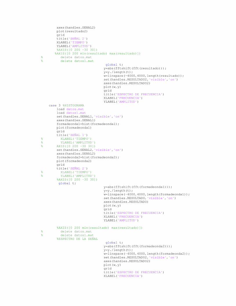
axes(handles.SENAL2) plot(resultado2) grid title('SEÑAL 2') XLABEL('TIEMPO') YLABEL('AMPLITUD') %AXIS([0 200 -30 30]) %AXIS([0 200 min(resultado) max(resultado)]) % delete datos.mat % delete datos1.mat global t; y=abs(fftshift(fft(resultado))); y=y./length(t); w=linspace(-4000,4000,length(resultado)); set(handles.RESULTADO2,'visible','on') axes(handles.RESULTADO2) plot(w,y) grid title('ESPECTRO DE FRECUENCIA') XLABEL('FRECUENCIA') YLABEL('AMPLITUD') case 3 %HISTOGRAMA load datos.mat load datos1.mat set(handles.SENAL1,'visible','on') axes(handles.SENAL1) formadeonda1=hist(formadeonda1); plot(formadeonda1) grid title('SEÑAL 1') % XLABEL('TIEMPO') % YLABEL('AMPLITUD') % AXIS([0 200 -30 30]) set(handles.SENAL2,'visible','on') axes(handles.SENAL2) formadeonda2=hist(formadeonda2); plot(formadeonda2) grid title('SEÑAL 2') % XLABEL('TIEMPO') % YLABEL('AMPLITUD') %AXIS([0 200 -30 30]) global t; y=abs(fftshift(fft(formadeonda1))); y=y./length(t); w=linspace(-4000,4000,length(formadeonda1)); set(handles.RESULTADO,'visible','on') axes(handles.RESULTADO) plot(w,y) grid title('ESPECTRO DE FRECUENCIA') XLABEL('FRECUENCIA') YLABEL('AMPLITUD') %AXIS([0 200 min(resultado) max(resultado)]) % delete datos.mat % delete datos1.mat %ESPECTRO DE LA SEÑAL global t; y=abs(fftshift(fft(formadeonda2))); y=y./length(t); w=linspace(-4000,4000,length(formadeonda2)); set(handles.RESULTADO2,'visible','on') axes(handles.RESULTADO2) plot(w,y) grid title('ESPECTRO DE FRECUENCIA') XLABEL('FRECUENCIA')

YLABEL('AMPLITUD') otherwise, end % Hints: contents = get(hObject,'String') returns OPERACION contents as cell array % contents{get(hObject,'Value')} returns selected item from OPERACION % --- Executes during object creation, after setting all properties. function OPERACION_CreateFcn(hObject, eventdata, handles) % hObject handle to OPERACION (see GCBO) % eventdata reserved - to be defined in a future version of MATLAB % handles empty - handles not created until after all CreateFcns called % Hint: popupmenu controls usually have a white background on Windows. % See ISPC and COMPUTER. if ispc && isequal(get(hObject,'BackgroundColor'), get(0,'defaultUicontrolBackgroundColor')) set(hObject,'BackgroundColor','white'); end % --- Executes on button press in REGRESAR. function REGRESAR_Callback(hObject, eventdata, handles) % hObject handle to REGRESAR (see GCBO) % eventdata reserved - to be defined in a future version of MATLAB % handles structure with handles and user data (see GUIDATA) r=get(handles.REGRESAR,'value'); if r==1, GENERACION1 end % --- Executes on button press in AYUDA. function AYUDA_Callback(hObject, eventdata, handles) % hObject handle to AYUDA (see GCBO) % eventdata reserved - to be defined in a future version of MATLAB % handles structure with handles and user data (see GUIDATA) r111=get(handles.AYUDA,'value'); if r111==1, open ('C:\Documents and Settings\javier\Mis documentos\TESIS_POSTGRADO\PARA LA TESIS\programas definitivos\ayudas\index_OTRASOPERACIONES.htm') end
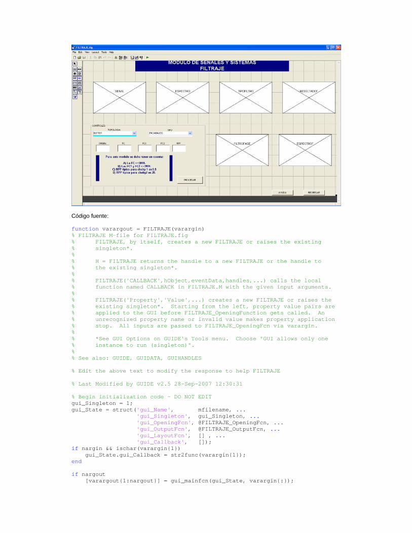
Código fuente: function varargout = FILTRAJE(varargin) % FILTRAJE M-file for FILTRAJE.fig % FILTRAJE, by itself, creates a new FILTRAJE or raises the existing % singleton*. % % H = FILTRAJE returns the handle to a new FILTRAJE or the handle to % the existing singleton*. % % FILTRAJE('CALLBACK',hObject,eventData,handles,...) calls the local % function named CALLBACK in FILTRAJE.M with the given input arguments. % % FILTRAJE('Property','Value',...) creates a new FILTRAJE or raises the % existing singleton*. Starting from the left, property value pairs are % applied to the GUI before FILTRAJE_OpeningFunction gets called. An % unrecognized property name or invalid value makes property application % stop. All inputs are passed to FILTRAJE_OpeningFcn via varargin. % % *See GUI Options on GUIDE's Tools menu. Choose "GUI allows only one % instance to run (singleton)". % % See also: GUIDE, GUIDATA, GUIHANDLES % Edit the above text to modify the response to help FILTRAJE % Last Modified by GUIDE v2.5 28-Sep-2007 12:30:31 % Begin initialization code - DO NOT EDIT gui_Singleton = 1; gui_State = struct('gui_Name', mfilename, ... 'gui_Singleton', gui_Singleton, ... 'gui_OpeningFcn', @FILTRAJE_OpeningFcn, ... 'gui_OutputFcn', @FILTRAJE_OutputFcn, ... 'gui_LayoutFcn', [] , ... 'gui_Callback', []); if nargin && ischar(varargin{1}) gui_State.gui_Callback = str2func(varargin{1}); end if nargout [varargout{1:nargout}] = gui_mainfcn(gui_State, varargin{:});

else gui_mainfcn(gui_State, varargin{:}); end % End initialization code - DO NOT EDIT % --- Executes just before FILTRAJE is made visible. function FILTRAJE_OpeningFcn(hObject, eventdata, handles, varargin) % This function has no output args, see OutputFcn. % hObject handle to figure % eventdata reserved - to be defined in a future version of MATLAB % handles structure with handles and user data (see GUIDATA) % varargin command line arguments to FILTRAJE (see VARARGIN) % Choose default command line output for FILTRAJE handles.output = hObject; % Update handles structure guidata(hObject, handles); % UIWAIT makes FILTRAJE wait for user response (see UIRESUME) % uiwait(handles.figure1); % --- Outputs from this function are returned to the command line. function varargout = FILTRAJE_OutputFcn(hObject, eventdata, handles) % varargout cell array for returning output args (see VARARGOUT); % hObject handle to figure % eventdata reserved - to be defined in a future version of MATLAB % handles structure with handles and user data (see GUIDATA) % Get default command line output from handles structure varargout{1} = handles.output; % --- Executes on button press in PROCESAR. function PROCESAR_Callback(hObject, eventdata, handles) % hObject handle to PROCESAR (see GCBO) % eventdata reserved - to be defined in a future version of MATLAB % handles structure with handles and user data (see GUIDATA) p=get(handles.PROCESAR,'value'); if p==1, topo=get(handles.TOPOLOGIA,'value'); switch topo case 1 %buterr tipo=get(handles.TIPOF,'value'); switch tipo case 1 %pasabajos set(handles.FC1,'visible','off') set(handles.FC11,'visible','off') set(handles.FC2,'visible','off') set(handles.FC22,'visible','off') set(handles.RIPLE1,'visible','off') set(handles.RIPLE,'visible','off') load datos.mat set(handles.SENAL,'visible','on') axes(handles.SENAL) plot(formadeonda1) grid title('SEÑAL A FILTRAR ') XLABEL('TIEMPO') YLABEL('AMPLITUD') %PARA EL ESPECTRO y1=abs(fftshift(fft(formadeonda1))); y1=y1./length(formadeonda1);

w=linspace(-4000,4000,length(formadeonda1)); set(handles.ESPECTRO,'visible','on') axes(handles.ESPECTRO) plot(w,y1) grid title('ESPECTRO DE FRECUENCIA') XLABEL('FRECUENCIA') YLABEL('AMPLITUD') %FILTRO N=str2double(get(handles.ORDENF,'String')); %validacion if isnan(N) beep set(handles.ORDENF,'String',1); N=1; errordlg('El valor debe ser numérico','ERROR') end if (N<=0)|(N>20) beep set(handles.ORDENF,'String',1); N=1; errordlg('El valor del orden del filtro debe ser mayor que "0" y menor que "21" ','ERROR') end Wn=str2double(get(handles.FCORTE,'String')); if isnan(Wn) beep set(handles.FCORTE,'String',0); Wn=0; errordlg('El valor debe ser numérico','ERROR') end if (Wn<=0)|(Wn>3999) beep set(handles.FCORTE,'String',1); Wn=1; errordlg('El valor de la frecuencia de corte del filtro debe ser mayor que "0" y menor que "3999Hz" ','ERROR') end Wn=Wn/4000; [B,A] = BUTTER(N,Wn); senalf=freqz(B,A,255,10000); senalf1=filter(B,A,formadeonda1); set(handles.TIPOFILTRO,'visible','on') axes(handles.TIPOFILTRO) semilogy (abs(senalf),'b'); grid title('DIAGRAMA DE BODE') XLABEL('FRECUENCIA') YLABEL('MAGNITUD') set(handles.FILTROFASE,'visible','on') axes(handles.FILTROFASE) plot(unwrap(angle(senalf))); grid title('DIAGRAMA DE BODE') XLABEL('FRECUENCIA') YLABEL('FASE') set(handles.RESULTADOF,'visible','on') axes(handles.RESULTADOF) plot(senalf1) grid title('RESULTADO') XLABEL('TIEMPO') YLABEL('AMPLITUD') %PARA EL ESPECTRO y2=abs(fftshift(fft(senalf1)));
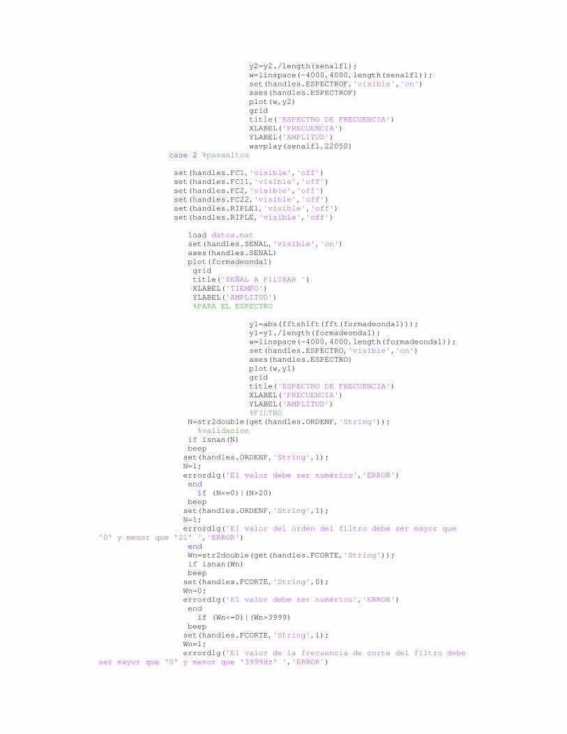
y2=y2./length(senalf1); w=linspace(-4000,4000,length(senalf1)); set(handles.ESPECTROF,'visible','on') axes(handles.ESPECTROF) plot(w,y2) grid title('ESPECTRO DE FRECUENCIA') XLABEL('FRECUENCIA') YLABEL('AMPLITUD') wavplay(senalf1,22050) case 2 %pasaaltos set(handles.FC1,'visible','off') set(handles.FC11,'visible','off') set(handles.FC2,'visible','off') set(handles.FC22,'visible','off') set(handles.RIPLE1,'visible','off') set(handles.RIPLE,'visible','off') load datos.mat set(handles.SENAL,'visible','on') axes(handles.SENAL) plot(formadeonda1) grid title('SEÑAL A FILTRAR ') XLABEL('TIEMPO') YLABEL('AMPLITUD') %PARA EL ESPECTRO y1=abs(fftshift(fft(formadeonda1))); y1=y1./length(formadeonda1); w=linspace(-4000,4000,length(formadeonda1)); set(handles.ESPECTRO,'visible','on') axes(handles.ESPECTRO) plot(w,y1) grid title('ESPECTRO DE FRECUENCIA') XLABEL('FRECUENCIA') YLABEL('AMPLITUD') %FILTRO N=str2double(get(handles.ORDENF,'String')); %validacion if isnan(N) beep set(handles.ORDENF,'String',1); N=1; errordlg('El valor debe ser numérico','ERROR') end if (N<=0)|(N>20) beep set(handles.ORDENF,'String',1); N=1; errordlg('El valor del orden del filtro debe ser mayor que "0" y menor que "21" ','ERROR') end Wn=str2double(get(handles.FCORTE,'String')); if isnan(Wn) beep set(handles.FCORTE,'String',0); Wn=0; errordlg('El valor debe ser numérico','ERROR') end if (Wn<=0)|(Wn>3999) beep set(handles.FCORTE,'String',1); Wn=1; errordlg('El valor de la frecuencia de corte del filtro debe ser mayor que "0" y menor que "3999Hz" ','ERROR')

end Wn=Wn/4000; [B,A] = BUTTER(N,Wn,'high'); senalf=freqz(B,A,255,10000); senalf1=filter(B,A,formadeonda1); set(handles.TIPOFILTRO,'visible','on') axes(handles.TIPOFILTRO) semilogy (abs(senalf),'b'); grid title('DIAGRAMA DE BODE') XLABEL('FRECUENCIA') YLABEL('MAGNITUD') set(handles.FILTROFASE,'visible','on') axes(handles.FILTROFASE) plot(unwrap(angle(senalf))); grid title('DIAGRAMA DE BODE') XLABEL('FRECUENCIA') YLABEL('FASE') set(handles.RESULTADOF,'visible','on') axes(handles.RESULTADOF) plot(senalf1) grid title('RESULTADO') XLABEL('TIEMPO') YLABEL('AMPLITUD') %PARA EL ESPECTRO y2=abs(fftshift(fft(senalf1))); y2=y2./length(senalf1); w=linspace(-4000,4000,length(senalf1)); set(handles.ESPECTROF,'visible','on') axes(handles.ESPECTROF) plot(w,y2) grid title('ESPECTRO DE FRECUENCIA') XLABEL('FRECUENCIA') YLABEL('AMPLITUD') wavplay(senalf1,22050) case 3 %pasabanda set(handles.FC1,'visible','on') set(handles.FC11,'visible','on') set(handles.FC2,'visible','on') set(handles.FC22,'visible','on') set(handles.RIPLE1,'visible','off') set(handles.RIPLE,'visible','off') load datos.mat set(handles.SENAL,'visible','on') axes(handles.SENAL) plot(formadeonda1) grid title('SEÑAL A FILTRAR ') XLABEL('TIEMPO') YLABEL('AMPLITUD') %PARA EL ESPECTRO y1=abs(fftshift(fft(formadeonda1))); y1=y1./length(formadeonda1); w=linspace(-4000,4000,length(formadeonda1)); set(handles.ESPECTRO,'visible','on') axes(handles.ESPECTRO) plot(w,y1) grid title('ESPECTRO DE FRECUENCIA')

XLABEL('FRECUENCIA') YLABEL('AMPLITUD') %FILTRO N=str2double(get(handles.ORDENF,'String')); %validacion if isnan(N) beep set(handles.ORDENF,'String',1); N=1; errordlg('El valor debe ser numérico','ERROR') end if (N<=0)|(N>20) beep set(handles.ORDENF,'String',1); N=1; errordlg('El valor del orden del filtro debe ser mayor que "0" y menor que "21" ','ERROR') end Wn1=str2double(get(handles.FC1,'String')); if isnan(Wn1) beep set(handles.FC1,'String',0); Wn1=0; errordlg('El valor debe ser numérico','ERROR') end if (Wn1<=0)|(Wn1>3999) beep set(handles.FC1,'String',1); Wn1=1; errordlg('El valor de la frecuencia de corte del filtro debe ser mayor que "0" y menor que "3999Hz" ','ERROR') end Wn1=Wn1/4000; Wn2=str2double(get(handles.FC2,'String')); if isnan(Wn2) beep set(handles.FC2,'String',1); Wn2=1; errordlg('El valor debe ser numérico','ERROR') end if (Wn2<=0)|(Wn2>3999) beep set(handles.FC2,'String',1); Wn2=1; errordlg('El valor de la frecuencia de corte del filtro debe ser mayor que "0" y menor que "3999Hz" ','ERROR') end Wn2=Wn2/4000; Wn=[Wn1 Wn2]; [B,A] = BUTTER(N,Wn); senalf=freqz(B,A,255,10000); senalf1=filter(B,A,formadeonda1); set(handles.TIPOFILTRO,'visible','on') axes(handles.TIPOFILTRO) semilogy (abs(senalf),'b'); grid title('DIAGRAMA DE BODE') XLABEL('FRECUENCIA') YLABEL('MAGNITUD') set(handles.FILTROFASE,'visible','on') axes(handles.FILTROFASE) plot(unwrap(angle(senalf))); grid title('DIAGRAMA DE BODE') XLABEL('FRECUENCIA')

YLABEL('FASE') set(handles.RESULTADOF,'visible','on') axes(handles.RESULTADOF) plot(senalf1) grid title('RESULTADO') XLABEL('TIEMPO') YLABEL('AMPLITUD') %PARA EL ESPECTRO y2=abs(fftshift(fft(senalf1))); y2=y2./length(senalf1); w=linspace(-4000,4000,length(senalf1)); set(handles.ESPECTROF,'visible','on') axes(handles.ESPECTROF) plot(w,y2) grid title('ESPECTRO DE FRECUENCIA') XLABEL('FRECUENCIA') YLABEL('AMPLITUD') wavplay(senalf1,22050) case 4 %rechazabanda set(handles.FC1,'visible','on') set(handles.FC11,'visible','on') set(handles.FC2,'visible','on') set(handles.FC22,'visible','on') set(handles.RIPLE1,'visible','off') set(handles.RIPLE,'visible','off') load datos.mat set(handles.SENAL,'visible','on') axes(handles.SENAL) plot(formadeonda1) grid title('SEÑAL A FILTRAR ') XLABEL('TIEMPO') YLABEL('AMPLITUD') %PARA EL ESPECTRO y1=abs(fftshift(fft(formadeonda1))); y1=y1./length(formadeonda1); w=linspace(-4000,4000,length(formadeonda1)); set(handles.ESPECTRO,'visible','on') axes(handles.ESPECTRO) plot(w,y1) grid title('ESPECTRO DE FRECUENCIA') XLABEL('FRECUENCIA') YLABEL('AMPLITUD') %FILTRO N=str2double(get(handles.ORDENF,'String')); %validacion if isnan(N) beep set(handles.ORDENF,'String',1); N=1; errordlg('El valor debe ser numérico','ERROR') end if (N<=0)|(N>20) beep set(handles.ORDENF,'String',1); N=1; errordlg('El valor del orden del filtro debe ser mayor que "0" y menor que "21" ','ERROR') end Wn1=str2double(get(handles.FC1,'String')); if isnan(Wn1) beep
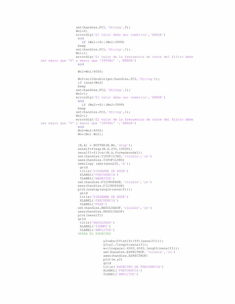
set(handles.FC1,'String',0); Wn1=0; errordlg('El valor debe ser numérico','ERROR') end if (Wn1<=0)|(Wn1>3999) beep set(handles.FC1,'String',1); Wn1=1; errordlg('El valor de la frecuencia de corte del filtro debe ser mayor que "0" y menor que "3999Hz" ','ERROR') end Wn1=Wn1/4000; Wn2=str2double(get(handles.FC2,'String')); if isnan(Wn2) beep set(handles.FC2,'String',1); Wn2=1; errordlg('El valor debe ser numérico','ERROR') end if (Wn2<=0)|(Wn2>3999) beep set(handles.FC2,'String',1); Wn2=1; errordlg('El valor de la frecuencia de corte del filtro debe ser mayor que "0" y menor que "3999Hz" ','ERROR') end Wn2=Wn2/4000; Wn=[Wn1 Wn2]; [B,A] = BUTTER(N,Wn,'stop'); senalf=freqz(B,A,255,10000); senalf1=filter(B,A,formadeonda1); set(handles.TIPOFILTRO,'visible','on') axes(handles.TIPOFILTRO) semilogy (abs(senalf),'b'); grid title('DIAGRAMA DE BODE') XLABEL('FRECUENCIA') YLABEL('MAGNITUD') set(handles.FILTROFASE,'visible','on') axes(handles.FILTROFASE) plot(unwrap(angle(senalf))); grid title('DIAGRAMA DE BODE') XLABEL('FRECUENCIA') YLABEL('FASE') set(handles.RESULTADOF,'visible','on') axes(handles.RESULTADOF) plot(senalf1) grid title('RESULTADO') XLABEL('TIEMPO') YLABEL('AMPLITUD') %PARA EL ESPECTRO y2=abs(fftshift(fft(senalf1))); y2=y2./length(senalf1); w=linspace(-4000,4000,length(senalf1)); set(handles.ESPECTROF,'visible','on') axes(handles.ESPECTROF) plot(w,y2) grid title('ESPECTRO DE FRECUENCIA') XLABEL('FRECUENCIA') YLABEL('AMPLITUD')

wavplay(senalf1,22050) otherwise, end case 2 %chebyI tipo=get(handles.TIPOF,'value'); switch tipo case 1 %pasabajos set(handles.FC1,'visible','off') set(handles.FC11,'visible','off') set(handles.FC2,'visible','off') set(handles.FC22,'visible','off') set(handles.RIPLE1,'visible','on') set(handles.RIPLE,'visible','on') load datos.mat set(handles.SENAL,'visible','on') axes(handles.SENAL) plot(formadeonda1) grid title('SEÑAL A FILTRAR ') XLABEL('TIEMPO') YLABEL('AMPLITUD') %PARA EL ESPECTRO y1=abs(fftshift(fft(formadeonda1))); y1=y1./length(formadeonda1); w=linspace(-4000,4000,length(formadeonda1)); set(handles.ESPECTRO,'visible','on') axes(handles.ESPECTRO) plot(w,y1) grid title('ESPECTRO DE FRECUENCIA') XLABEL('FRECUENCIA') YLABEL('AMPLITUD') %FILTRO N=str2double(get(handles.ORDENF,'String')); %validacion if isnan(N) beep set(handles.ORDENF,'String',1); N=1; errordlg('El valor debe ser numérico','ERROR') end if (N<=0)|(N>20) beep set(handles.ORDENF,'String',1); N=1; errordlg('El valor del orden del filtro debe ser mayor que "0" y menor que "21" ','ERROR') end Wn=str2double(get(handles.FCORTE,'String')); if isnan(Wn) beep set(handles.FCORTE,'String',0); Wn=0; errordlg('El valor debe ser numérico','ERROR') end if (Wn<=0)|(Wn>3999) beep set(handles.FCORTE,'String',1); Wn=1; errordlg('El valor la frecuencia de corte del filtro debe ser mayor que "0" y menor que "3999Hz" ','ERROR')

end Wn=Wn/4000; R=str2double(get(handles.RIPLE,'String')); %validacion if isnan(R) beep set(handles.RIPLE,'String',0.5); R=0.5; errordlg('El valor debe ser numérico','ERROR') end [B,A] = CHEBY1(N,R,Wn); senalf=freqz(B,A,255,10000); senalf1=filter(B,A,formadeonda1); set(handles.TIPOFILTRO,'visible','on') axes(handles.TIPOFILTRO) semilogy (abs(senalf),'b'); grid title('DIAGRAMA DE BODE') XLABEL('FRECUENCIA') YLABEL('MAGNITUD') set(handles.FILTROFASE,'visible','on') axes(handles.FILTROFASE) plot(unwrap(angle(senalf))); grid title('DIAGRAMA DE BODE') XLABEL('FRECUENCIA') YLABEL('FASE') set(handles.RESULTADOF,'visible','on') axes(handles.RESULTADOF) plot(senalf1) grid title('RESULTADO') XLABEL('TIEMPO') YLABEL('AMPLITUD') %PARA EL ESPECTRO y2=abs(fftshift(fft(senalf1))); y2=y2./length(senalf1); w=linspace(-4000,4000,length(senalf1)); set(handles.ESPECTROF,'visible','on') axes(handles.ESPECTROF) plot(w,y2) grid title('ESPECTRO DE FRECUENCIA') XLABEL('FRECUENCIA') YLABEL('AMPLITUD') wavplay(senalf1,22050) case 2 %pasaaltos set(handles.FC1,'visible','off') set(handles.FC11,'visible','off') set(handles.FC2,'visible','off') set(handles.FC22,'visible','off') set(handles.RIPLE1,'visible','on') set(handles.RIPLE,'visible','on') load datos.mat set(handles.SENAL,'visible','on') axes(handles.SENAL) plot(formadeonda1) grid title('SEÑAL A FILTRAR ') XLABEL('TIEMPO') YLABEL('AMPLITUD') %PARA EL ESPECTRO

y1=abs(fftshift(fft(formadeonda1))); y1=y1./length(formadeonda1); w=linspace(-4000,4000,length(formadeonda1)); set(handles.ESPECTRO,'visible','on') axes(handles.ESPECTRO) plot(w,y1) grid title('ESPECTRO DE FRECUENCIA') XLABEL('FRECUENCIA') YLABEL('AMPLITUD') %FILTRO N=str2double(get(handles.ORDENF,'String')); %validacion if isnan(N) beep set(handles.ORDENF,'String',1); N=1; errordlg('El valor debe ser numérico','ERROR') end if (N<=0)|(N>20) beep set(handles.ORDENF,'String',1); N=1; errordlg('El valor del orden del filtro debe ser mayor que "0" y menor que "21" ','ERROR') end Wn=str2double(get(handles.FCORTE,'String')); if isnan(Wn) beep set(handles.FCORTE,'String',1); Wn=1; errordlg('El valor debe ser numérico','ERROR') end if (Wn<=0)|(Wn>3999) beep set(handles.FCORTE,'String',1); Wn=1; errordlg('El valor de la frecuencia de corte del filtro debe ser mayor que "0" y menor que "3999Hz" ','ERROR') end Wn=Wn/4000; R=str2double(get(handles.RIPLE,'String')); %validacion if isnan(R) beep set(handles.RIPLE,'String',0.5); R=0.5; errordlg('El valor debe ser numérico','ERROR') end [B,A] = CHEBY1(N,R,Wn,'high'); senalf=freqz(B,A,255,10000); senalf1=filter(B,A,formadeonda1); set(handles.TIPOFILTRO,'visible','on') axes(handles.TIPOFILTRO) semilogy (abs(senalf),'b'); grid title('DIAGRAMA DE BODE') XLABEL('FRECUENCIA') YLABEL('MAGNITUD') set(handles.FILTROFASE,'visible','on') axes(handles.FILTROFASE) plot(unwrap(angle(senalf))); grid title('DIAGRAMA DE BODE') XLABEL('FRECUENCIA') YLABEL('FASE')
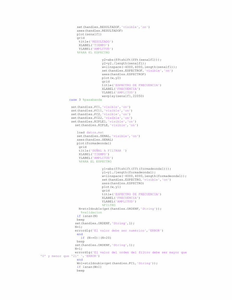
set(handles.RESULTADOF,'visible','on') axes(handles.RESULTADOF) plot(senalf1) grid title('RESULTADO') XLABEL('TIEMPO') YLABEL('AMPLITUD') %PARA EL ESPECTRO y2=abs(fftshift(fft(senalf1))); y2=y2./length(senalf1); w=linspace(-4000,4000,length(senalf1)); set(handles.ESPECTROF,'visible','on') axes(handles.ESPECTROF) plot(w,y2) grid title('ESPECTRO DE FRECUENCIA') XLABEL('FRECUENCIA') YLABEL('AMPLITUD') wavplay(senalf1,22050) case 3 %pasabanda set(handles.FC1,'visible','on') set(handles.FC11,'visible','on') set(handles.FC2,'visible','on') set(handles.FC22,'visible','on') set(handles.RIPLE1,'visible','on') set(handles.RIPLE,'visible','on') load datos.mat set(handles.SENAL,'visible','on') axes(handles.SENAL) plot(formadeonda1) grid title('SEÑAL A FILTRAR ') XLABEL('TIEMPO') YLABEL('AMPLITUD') %PARA EL ESPECTRO y1=abs(fftshift(fft(formadeonda1))); y1=y1./length(formadeonda1); w=linspace(-4000,4000,length(formadeonda1)); set(handles.ESPECTRO,'visible','on') axes(handles.ESPECTRO) plot(w,y1) grid title('ESPECTRO DE FRECUENCIA') XLABEL('FRECUENCIA') YLABEL('AMPLITUD') %FILTRO N=str2double(get(handles.ORDENF,'String')); %validacion if isnan(N) beep set(handles.ORDENF,'String',1); N=1; errordlg('El valor debe ser numérico','ERROR') end if (N<=0)|(N>20) beep set(handles.ORDENF,'String',1); N=1; errordlg('El valor del orden del filtro debe ser mayor que "0" y menor que "21" ','ERROR') end Wn1=str2double(get(handles.FC1,'String')); if isnan(Wn1) beep

set(handles.FC1,'String',1); Wn1=1; errordlg('El valor debe ser numérico','ERROR') end if (Wn1<=0)|(Wn1>3999) beep set(handles.FC1,'String',1); Wn1=1; errordlg('El valor del de la frecuencia de corte filtro debe ser mayor que "0" y menor que "3999Hz" ','ERROR') end Wn1=Wn1/4000; Wn2=str2double(get(handles.FC2,'String')); if isnan(Wn2) beep set(handles.FC2,'String',1); Wn2=1; errordlg('El valor debe ser numérico','ERROR') end if (Wn2<=0)|(Wn2>3999) beep set(handles.FC2,'String',1); Wn2=1; errordlg('El valor de la frecuencia de corte del filtro debe ser mayor que "0" y menor que "3999Hz" ','ERROR') end Wn2=Wn2/4000; Wn=[Wn1 Wn2]; R=str2double(get(handles.RIPLE,'String')); %validacion if isnan(R) beep set(handles.RIPLE,'String',0.5); R=0.5; errordlg('El valor debe ser numérico','ERROR') end [B,A] = CHEBY1(N,R,Wn); senalf=freqz(B,A,255,10000); senalf1=filter(B,A,formadeonda1); set(handles.TIPOFILTRO,'visible','on') axes(handles.TIPOFILTRO) semilogy (abs(senalf),'b'); grid title('DIAGRAMA DE BODE') XLABEL('FRECUENCIA') YLABEL('MAGNITUD') set(handles.FILTROFASE,'visible','on') axes(handles.FILTROFASE) plot(unwrap(angle(senalf))); grid title('DIAGRAMA DE BODE') XLABEL('FRECUENCIA') YLABEL('FASE') set(handles.RESULTADOF,'visible','on') axes(handles.RESULTADOF) plot(senalf1) grid title('RESULTADO') XLABEL('TIEMPO') YLABEL('AMPLITUD') %PARA EL ESPECTRO y2=abs(fftshift(fft(senalf1))); y2=y2./length(senalf1); w=linspace(-4000,4000,length(senalf1));

set(handles.ESPECTROF,'visible','on') axes(handles.ESPECTROF) plot(w,y2) grid title('ESPECTRO DE FRECUENCIA') XLABEL('FRECUENCIA') YLABEL('AMPLITUD') wavplay(senalf1,22050) case 4 %rechazabanda set(handles.FC1,'visible','on') set(handles.FC11,'visible','on') set(handles.FC2,'visible','on') set(handles.FC22,'visible','on') set(handles.RIPLE1,'visible','on') set(handles.RIPLE,'visible','on') load datos.mat set(handles.SENAL,'visible','on') axes(handles.SENAL) plot(formadeonda1) grid title('SEÑAL A FILTRAR ') XLABEL('TIEMPO') YLABEL('AMPLITUD') %PARA EL ESPECTRO y1=abs(fftshift(fft(formadeonda1))); y1=y1./length(formadeonda1); w=linspace(-4000,4000,length(formadeonda1)); set(handles.ESPECTRO,'visible','on') axes(handles.ESPECTRO) plot(w,y1) grid title('ESPECTRO DE FRECUENCIA') XLABEL('FRECUENCIA') YLABEL('AMPLITUD') %FILTRO N=str2double(get(handles.ORDENF,'String')); %validacion if isnan(N) beep set(handles.ORDENF,'String',1); N=1; errordlg('El valor debe ser numérico','ERROR') end if (N<=0)|(N>20) beep set(handles.ORDENF,'String',1); N=1; errordlg('El valor del orden del filtro debe ser mayor que "0" y menor que "21" ','ERROR') end Wn1=str2double(get(handles.FC1,'String')); if isnan(Wn1) beep set(handles.FC1,'String',1); Wn1=1; errordlg('El valor debe ser numérico','ERROR') end if (Wn1<=0)|(Wn1>3999) beep set(handles.FC1,'String',1); Wn1=1; errordlg('El valor de la frecuencia de corte del filtro debe ser mayor que "0" y menor que "3999Hz" ','ERROR') end
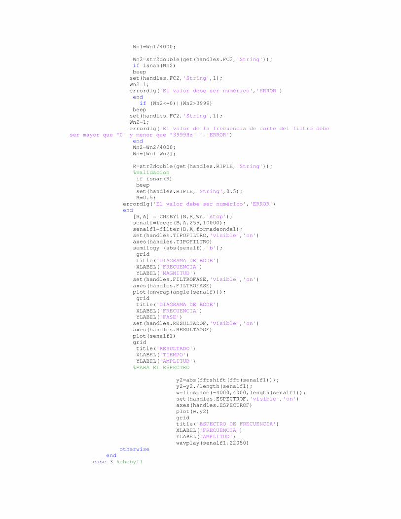
Wn1=Wn1/4000; Wn2=str2double(get(handles.FC2,'String')); if isnan(Wn2) beep set(handles.FC2,'String',1); Wn2=1; errordlg('El valor debe ser numérico','ERROR') end if (Wn2<=0)|(Wn2>3999) beep set(handles.FC2,'String',1); Wn2=1; errordlg('El valor de la frecuencia de corte del filtro debe ser mayor que "0" y menor que "3999Hz" ','ERROR') end Wn2=Wn2/4000; Wn=[Wn1 Wn2]; R=str2double(get(handles.RIPLE,'String')); %validacion if isnan(R) beep set(handles.RIPLE,'String',0.5); R=0.5; errordlg('El valor debe ser numérico','ERROR') end [B,A] = CHEBY1(N,R,Wn,'stop'); senalf=freqz(B,A,255,10000); senalf1=filter(B,A,formadeonda1); set(handles.TIPOFILTRO,'visible','on') axes(handles.TIPOFILTRO) semilogy (abs(senalf),'b'); grid title('DIAGRAMA DE BODE') XLABEL('FRECUENCIA') YLABEL('MAGNITUD') set(handles.FILTROFASE,'visible','on') axes(handles.FILTROFASE) plot(unwrap(angle(senalf))); grid title('DIAGRAMA DE BODE') XLABEL('FRECUENCIA') YLABEL('FASE') set(handles.RESULTADOF,'visible','on') axes(handles.RESULTADOF) plot(senalf1) grid title('RESULTADO') XLABEL('TIEMPO') YLABEL('AMPLITUD') %PARA EL ESPECTRO y2=abs(fftshift(fft(senalf1))); y2=y2./length(senalf1); w=linspace(-4000,4000,length(senalf1)); set(handles.ESPECTROF,'visible','on') axes(handles.ESPECTROF) plot(w,y2) grid title('ESPECTRO DE FRECUENCIA') XLABEL('FRECUENCIA') YLABEL('AMPLITUD') wavplay(senalf1,22050) otherwise end case 3 %chebyII

tipo=get(handles.TIPOF,'value'); switch tipo case 1 %pasabajos set(handles.FC1,'visible','off') set(handles.FC11,'visible','off') set(handles.FC2,'visible','off') set(handles.FC22,'visible','off') set(handles.RIPLE1,'visible','on') set(handles.RIPLE,'visible','on') load datos.mat set(handles.SENAL,'visible','on') axes(handles.SENAL) plot(formadeonda1) grid title('SEÑAL A FILTRAR ') XLABEL('TIEMPO') YLABEL('AMPLITUD') %PARA EL ESPECTRO y1=abs(fftshift(fft(formadeonda1))); y1=y1./length(formadeonda1); w=linspace(-4000,4000,length(formadeonda1)); set(handles.ESPECTRO,'visible','on') axes(handles.ESPECTRO) plot(w,y1) grid title('ESPECTRO DE FRECUENCIA') XLABEL('FRECUENCIA') YLABEL('AMPLITUD') %FILTRO N=str2double(get(handles.ORDENF,'String')); %validacion if isnan(N) beep set(handles.ORDENF,'String',1); N=1; errordlg('El valor debe ser numérico','ERROR') end if (N<=0)|(N>20) beep set(handles.ORDENF,'String',1); N=1; errordlg('El valor del orden del filtro debe ser mayor que "0" y menor que "21" ','ERROR') end Wn=str2double(get(handles.FCORTE,'String')); if isnan(Wn) beep set(handles.FCORTE,'String',1); Wn=1; errordlg('El valor debe ser numérico','ERROR') end if (Wn<=0)|(Wn>3999) beep set(handles.FCORTE,'String',1); Wn=1; errordlg('El valor de la frecuencia de corte del filtro debe ser mayor que "0" y menor que "3999Hz" ','ERROR') end Wn=Wn/4000; R=str2double(get(handles.RIPLE,'String')); %validacion if isnan(R) beep set(handles.RIPLE,'String',20);

R=20; errordlg('El valor debe ser numérico','ERROR') end [B,A] = CHEBY2(N,R,Wn); senalf=freqz(B,A,255,10000); senalf1=filter(B,A,formadeonda1); set(handles.TIPOFILTRO,'visible','on') axes(handles.TIPOFILTRO) semilogy (abs(senalf),'b'); grid title('DIAGRAMA DE BODE') XLABEL('FRECUENCIA') YLABEL('MAGNITUD') set(handles.FILTROFASE,'visible','on') axes(handles.FILTROFASE) plot(unwrap(angle(senalf))); grid title('DIAGRAMA DE BODE') XLABEL('FRECUENCIA') YLABEL('FASE') set(handles.RESULTADOF,'visible','on') axes(handles.RESULTADOF) plot(senalf1) grid title('RESULTADO') XLABEL('TIEMPO') YLABEL('AMPLITUD') %PARA EL ESPECTRO y2=abs(fftshift(fft(senalf1))); y2=y2./length(senalf1); w=linspace(-4000,4000,length(senalf1)); set(handles.ESPECTROF,'visible','on') axes(handles.ESPECTROF) plot(w,y2) grid title('ESPECTRO DE FRECUENCIA') XLABEL('FRECUENCIA') YLABEL('AMPLITUD') wavplay(senalf1,22050) case 2 %pasaaltos set(handles.FC1,'visible','off') set(handles.FC11,'visible','off') set(handles.FC2,'visible','off') set(handles.FC22,'visible','off') set(handles.RIPLE1,'visible','on') set(handles.RIPLE,'visible','on') load datos.mat set(handles.SENAL,'visible','on') axes(handles.SENAL) plot(formadeonda1) grid title('SEÑAL A FILTRAR ') XLABEL('TIEMPO') YLABEL('AMPLITUD') %PARA EL ESPECTRO y1=abs(fftshift(fft(formadeonda1))); y1=y1./length(formadeonda1); w=linspace(-4000,4000,length(formadeonda1)); set(handles.ESPECTRO,'visible','on') axes(handles.ESPECTRO) plot(w,y1) grid title('ESPECTRO DE FRECUENCIA') XLABEL('FRECUENCIA')

YLABEL('AMPLITUD') %FILTRO N=str2double(get(handles.ORDENF,'String')); %validacion if isnan(N) beep set(handles.ORDENF,'String',1); N=1; errordlg('El valor debe ser numérico','ERROR') end if (N<=0)|(N>20) beep set(handles.ORDENF,'String',1); N=1; errordlg('El valor del orden del filtro debe ser mayor que "0" y menor que "21" ','ERROR') end Wn=str2double(get(handles.FCORTE,'String')); if isnan(Wn) beep set(handles.FCORTE,'String',1); Wn=1; errordlg('El valor debe ser numérico','ERROR') end if (Wn<=0)|(Wn>3999) beep set(handles.FCORTE,'String',1); Wn=1; errordlg('El valor de la frecuencia de corte del filtro debe ser mayor que "0" y menor que "3999Hz" ','ERROR') end Wn=Wn/4000; R=str2double(get(handles.RIPLE,'String')); %validacion if isnan(R) beep set(handles.RIPLE,'String',20); R=20; errordlg('El valor debe ser numérico','ERROR') end [B,A] = CHEBY2(N,R,Wn,'high'); senalf=freqz(B,A,255,10000); senalf1=filter(B,A,formadeonda1); set(handles.TIPOFILTRO,'visible','on') axes(handles.TIPOFILTRO) semilogy (abs(senalf),'b'); grid title('DIAGRAMA DE BODE') XLABEL('FRECUENCIA') YLABEL('MAGNITUD') set(handles.FILTROFASE,'visible','on') axes(handles.FILTROFASE) plot(unwrap(angle(senalf))); grid title('DIAGRAMA DE BODE') XLABEL('FRECUENCIA') YLABEL('FASE') set(handles.RESULTADOF,'visible','on') axes(handles.RESULTADOF) plot(senalf1) grid title('RESULTADO') XLABEL('TIEMPO') YLABEL('AMPLITUD') %PARA EL ESPECTRO

y2=abs(fftshift(fft(senalf1))); y2=y2./length(senalf1); w=linspace(-4000,4000,length(senalf1)); set(handles.ESPECTROF,'visible','on') axes(handles.ESPECTROF) plot(w,y2) grid title('ESPECTRO DE FRECUENCIA') XLABEL('FRECUENCIA') YLABEL('AMPLITUD') wavplay(senalf1,22050) case 3 %pasabanda set(handles.FC1,'visible','on') set(handles.FC11,'visible','on') set(handles.FC2,'visible','on') set(handles.FC22,'visible','on') set(handles.RIPLE1,'visible','on') set(handles.RIPLE,'visible','on') load datos.mat set(handles.SENAL,'visible','on') axes(handles.SENAL) plot(formadeonda1) grid title('SEÑAL A FILTRAR ') XLABEL('TIEMPO') YLABEL('AMPLITUD') %PARA EL ESPECTRO y1=abs(fftshift(fft(formadeonda1))); y1=y1./length(formadeonda1); w=linspace(-4000,4000,length(formadeonda1)); set(handles.ESPECTRO,'visible','on') axes(handles.ESPECTRO) plot(w,y1) grid title('ESPECTRO DE FRECUENCIA') XLABEL('FRECUENCIA') YLABEL('AMPLITUD') %FILTRO N=str2double(get(handles.ORDENF,'String')); %validacion if isnan(N) beep set(handles.ORDENF,'String',1); N=1; errordlg('El valor debe ser numérico','ERROR') end if (N<=0)|(N>20) beep set(handles.ORDENF,'String',1); N=1; errordlg('El valor del orden del filtro debe ser mayor que "0" y menor que "21" ','ERROR') end Wn1=str2double(get(handles.FC1,'String')); if isnan(Wn1) beep set(handles.FC1,'String',1); Wn1=1; errordlg('El valor debe ser numérico','ERROR') end if (Wn1<=0)|(Wn1>3999) beep set(handles.FC1,'String',1); Wn1=1;

errordlg('El valor de la frecuencia de corte del filtro debe ser mayor que "0" y menor que "3999Hz" ','ERROR') end Wn1=Wn1/4000; Wn2=str2double(get(handles.FC2,'String')); if isnan(Wn2) beep set(handles.FC2,'String',1); Wn2=1; errordlg('El valor debe ser numérico','ERROR') end if (Wn2<=0)|(Wn2>3999) beep set(handles.FC2,'String',1); Wn2=1; errordlg('El valor de la frecuencia de corte del filtro debe ser mayor que "0" y menor que "3999Hz" ','ERROR') end Wn2=Wn2/4000; Wn=[Wn1 Wn2]; R=str2double(get(handles.RIPLE,'String')); %validacion if isnan(R) beep set(handles.RIPLE,'String',20); R=20; errordlg('El valor debe ser numérico','ERROR') end [B,A] = CHEBY2(N,R,Wn); senalf=freqz(B,A,255,10000); senalf1=filter(B,A,formadeonda1); set(handles.TIPOFILTRO,'visible','on') axes(handles.TIPOFILTRO) semilogy (abs(senalf),'b'); grid title('DIAGRAMA DE BODE') XLABEL('FRECUENCIA') YLABEL('MAGNITUD') set(handles.FILTROFASE,'visible','on') axes(handles.FILTROFASE) plot(unwrap(angle(senalf))); grid title('DIAGRAMA DE BODE') XLABEL('FRECUENCIA') YLABEL('FASE') set(handles.RESULTADOF,'visible','on') axes(handles.RESULTADOF) plot(senalf1) grid title('RESULTADO') XLABEL('TIEMPO') YLABEL('AMPLITUD') %PARA EL ESPECTRO y2=abs(fftshift(fft(senalf1))); y2=y2./length(senalf1); w=linspace(-4000,4000,length(senalf1)); set(handles.ESPECTROF,'visible','on') axes(handles.ESPECTROF) plot(w,y2) grid title('ESPECTRO DE FRECUENCIA') XLABEL('FRECUENCIA') YLABEL('AMPLITUD')
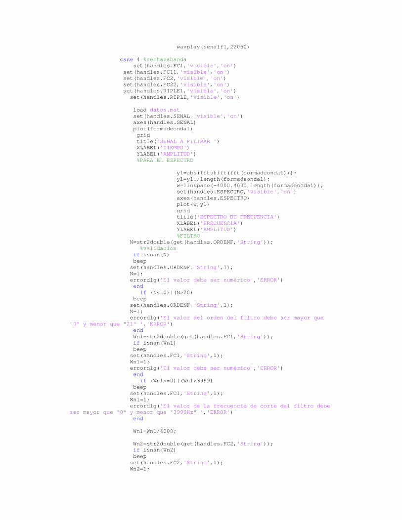
wavplay(senalf1,22050) case 4 %rechazabanda set(handles.FC1,'visible','on') set(handles.FC11,'visible','on') set(handles.FC2,'visible','on') set(handles.FC22,'visible','on') set(handles.RIPLE1,'visible','on') set(handles.RIPLE,'visible','on') load datos.mat set(handles.SENAL,'visible','on') axes(handles.SENAL) plot(formadeonda1) grid title('SEÑAL A FILTRAR ') XLABEL('TIEMPO') YLABEL('AMPLITUD') %PARA EL ESPECTRO y1=abs(fftshift(fft(formadeonda1))); y1=y1./length(formadeonda1); w=linspace(-4000,4000,length(formadeonda1)); set(handles.ESPECTRO,'visible','on') axes(handles.ESPECTRO) plot(w,y1) grid title('ESPECTRO DE FRECUENCIA') XLABEL('FRECUENCIA') YLABEL('AMPLITUD') %FILTRO N=str2double(get(handles.ORDENF,'String')); %validacion if isnan(N) beep set(handles.ORDENF,'String',1); N=1; errordlg('El valor debe ser numérico','ERROR') end if (N<=0)|(N>20) beep set(handles.ORDENF,'String',1); N=1; errordlg('El valor del orden del filtro debe ser mayor que "0" y menor que "21" ','ERROR') end Wn1=str2double(get(handles.FC1,'String')); if isnan(Wn1) beep set(handles.FC1,'String',1); Wn1=1; errordlg('El valor debe ser numérico','ERROR') end if (Wn1<=0)|(Wn1>3999) beep set(handles.FC1,'String',1); Wn1=1; errordlg('El valor de la frecuencia de corte del filtro debe ser mayor que "0" y menor que "3999Hz" ','ERROR') end Wn1=Wn1/4000; Wn2=str2double(get(handles.FC2,'String')); if isnan(Wn2) beep set(handles.FC2,'String',1); Wn2=1;

errordlg('El valor debe ser numérico','ERROR') end if (Wn2<=0)|(Wn2>3999) beep set(handles.FC2,'String',1); Wn2=1; errordlg('El valor de la frecuencia de corte del filtro debe ser mayor que "0" y menor que "3999Hz" ','ERROR') end Wn2=Wn2/4000; Wn=[Wn1 Wn2]; R=str2double(get(handles.RIPLE,'String')); %validacion if isnan(R) beep set(handles.RIPLE,'String',20); R=20; errordlg('El valor debe ser numérico','ERROR') end [B,A] = CHEBY2(N,R,Wn,'stop'); senalf=freqz(B,A,255,10000); senalf1=filter(B,A,formadeonda1); set(handles.TIPOFILTRO,'visible','on') axes(handles.TIPOFILTRO) semilogy (abs(senalf),'b'); grid title('DIAGRAMA DE BODE') XLABEL('FRECUENCIA') YLABEL('MAGNITUD') set(handles.FILTROFASE,'visible','on') axes(handles.FILTROFASE) plot(unwrap(angle(senalf))); grid title('DIAGRAMA DE BODE') XLABEL('FRECUENCIA') YLABEL('FASE') set(handles.RESULTADOF,'visible','on') axes(handles.RESULTADOF) plot(senalf1) grid title('RESULTADO') XLABEL('TIEMPO') YLABEL('AMPLITUD') %PARA EL ESPECTRO y2=abs(fftshift(fft(senalf1))); y2=y2./length(senalf1); w=linspace(-4000,4000,length(senalf1)); set(handles.ESPECTROF,'visible','on') axes(handles.ESPECTROF) plot(w,y2) grid title('ESPECTRO DE FRECUENCIA') XLABEL('FRECUENCIA') YLABEL('AMPLITUD') wavplay(senalf1,22050) otherwise end otherwise, end end

% --- Executes on selection change in listbox1. function listbox1_Callback(hObject, eventdata, handles) % hObject handle to listbox1 (see GCBO) % eventdata reserved - to be defined in a future version of MATLAB % handles structure with handles and user data (see GUIDATA) % Hints: contents = get(hObject,'String') returns listbox1 contents as cell array % contents{get(hObject,'Value')} returns selected item from listbox1 % --- Executes during object creation, after setting all properties. function listbox1_CreateFcn(hObject, eventdata, handles) % hObject handle to listbox1 (see GCBO) % eventdata reserved - to be defined in a future version of MATLAB % handles empty - handles not created until after all CreateFcns called % Hint: listbox controls usually have a white background on Windows. % See ISPC and COMPUTER. if ispc && isequal(get(hObject,'BackgroundColor'), get(0,'defaultUicontrolBackgroundColor')) set(hObject,'BackgroundColor','white'); end % --- Executes on selection change in TOPOLOGIA. function TOPOLOGIA_Callback(hObject, eventdata, handles) % hObject handle to TOPOLOGIA (see GCBO) % eventdata reserved - to be defined in a future version of MATLAB % handles structure with handles and user data (see GUIDATA) % Hints: contents = get(hObject,'String') returns TOPOLOGIA contents as cell array % contents{get(hObject,'Value')} returns selected item from TOPOLOGIA % --- Executes during object creation, after setting all properties. function TOPOLOGIA_CreateFcn(hObject, eventdata, handles) % hObject handle to TOPOLOGIA (see GCBO) % eventdata reserved - to be defined in a future version of MATLAB % handles empty - handles not created until after all CreateFcns called % Hint: popupmenu controls usually have a white background on Windows. % See ISPC and COMPUTER. if ispc && isequal(get(hObject,'BackgroundColor'), get(0,'defaultUicontrolBackgroundColor')) set(hObject,'BackgroundColor','white'); end % --- Executes on selection change in TIPOF. function TIPOF_Callback(hObject, eventdata, handles) % hObject handle to TIPOF (see GCBO) % eventdata reserved - to be defined in a future version of MATLAB % handles structure with handles and user data (see GUIDATA) % Hints: contents = get(hObject,'String') returns TIPOF contents as cell array % contents{get(hObject,'Value')} returns selected item from TIPOF % --- Executes during object creation, after setting all properties. function TIPOF_CreateFcn(hObject, eventdata, handles) % hObject handle to TIPOF (see GCBO) % eventdata reserved - to be defined in a future version of MATLAB % handles empty - handles not created until after all CreateFcns called

% Hint: popupmenu controls usually have a white background on Windows. % See ISPC and COMPUTER. if ispc && isequal(get(hObject,'BackgroundColor'), get(0,'defaultUicontrolBackgroundColor')) set(hObject,'BackgroundColor','white'); end function ORDENF_Callback(hObject, eventdata, handles) % hObject handle to ORDENF (see GCBO) % eventdata reserved - to be defined in a future version of MATLAB % handles structure with handles and user data (see GUIDATA) % Hints: get(hObject,'String') returns contents of ORDENF as text % str2double(get(hObject,'String')) returns contents of ORDENF as a double % --- Executes during object creation, after setting all properties. function ORDENF_CreateFcn(hObject, eventdata, handles) % hObject handle to ORDENF (see GCBO) % eventdata reserved - to be defined in a future version of MATLAB % handles empty - handles not created until after all CreateFcns called % Hint: edit controls usually have a white background on Windows. % See ISPC and COMPUTER. if ispc && isequal(get(hObject,'BackgroundColor'), get(0,'defaultUicontrolBackgroundColor')) set(hObject,'BackgroundColor','white'); end function FCORTE_Callback(hObject, eventdata, handles) % hObject handle to FCORTE (see GCBO) % eventdata reserved - to be defined in a future version of MATLAB % handles structure with handles and user data (see GUIDATA) % Hints: get(hObject,'String') returns contents of FCORTE as text % str2double(get(hObject,'String')) returns contents of FCORTE as a double % --- Executes during object creation, after setting all properties. function FCORTE_CreateFcn(hObject, eventdata, handles) % hObject handle to FCORTE (see GCBO) % eventdata reserved - to be defined in a future version of MATLAB % handles empty - handles not created until after all CreateFcns called % Hint: edit controls usually have a white background on Windows. % See ISPC and COMPUTER. if ispc && isequal(get(hObject,'BackgroundColor'), get(0,'defaultUicontrolBackgroundColor')) set(hObject,'BackgroundColor','white'); end function FC1_Callback(hObject, eventdata, handles) % hObject handle to FC1 (see GCBO) % eventdata reserved - to be defined in a future version of MATLAB % handles structure with handles and user data (see GUIDATA) % Hints: get(hObject,'String') returns contents of FC1 as text % str2double(get(hObject,'String')) returns contents of FC1 as a double

% --- Executes during object creation, after setting all properties. function FC1_CreateFcn(hObject, eventdata, handles) % hObject handle to FC1 (see GCBO) % eventdata reserved - to be defined in a future version of MATLAB % handles empty - handles not created until after all CreateFcns called % Hint: edit controls usually have a white background on Windows. % See ISPC and COMPUTER. if ispc && isequal(get(hObject,'BackgroundColor'), get(0,'defaultUicontrolBackgroundColor')) set(hObject,'BackgroundColor','white'); end function FC2_Callback(hObject, eventdata, handles) % hObject handle to FC2 (see GCBO) % eventdata reserved - to be defined in a future version of MATLAB % handles structure with handles and user data (see GUIDATA) % Hints: get(hObject,'String') returns contents of FC2 as text % str2double(get(hObject,'String')) returns contents of FC2 as a double % --- Executes during object creation, after setting all properties. function FC2_CreateFcn(hObject, eventdata, handles) % hObject handle to FC2 (see GCBO) % eventdata reserved - to be defined in a future version of MATLAB % handles empty - handles not created until after all CreateFcns called % Hint: edit controls usually have a white background on Windows. % See ISPC and COMPUTER. if ispc && isequal(get(hObject,'BackgroundColor'), get(0,'defaultUicontrolBackgroundColor')) set(hObject,'BackgroundColor','white'); end % --- Executes on button press in REGRESAR. function REGRESAR_Callback(hObject, eventdata, handles) % hObject handle to REGRESAR (see GCBO) % eventdata reserved - to be defined in a future version of MATLAB % handles structure with handles and user data (see GUIDATA) R=get(handles.REGRESAR,'value'); if R==1, GENERACION1 end function edit6_Callback(hObject, eventdata, handles) % hObject handle to edit6 (see GCBO) % eventdata reserved - to be defined in a future version of MATLAB % handles structure with handles and user data (see GUIDATA) % Hints: get(hObject,'String') returns contents of edit6 as text % str2double(get(hObject,'String')) returns contents of edit6 as a double % --- Executes during object creation, after setting all properties. function edit6_CreateFcn(hObject, eventdata, handles) % hObject handle to edit6 (see GCBO) % eventdata reserved - to be defined in a future version of MATLAB % handles empty - handles not created until after all CreateFcns called

% Hint: edit controls usually have a white background on Windows. % See ISPC and COMPUTER. if ispc && isequal(get(hObject,'BackgroundColor'), get(0,'defaultUicontrolBackgroundColor')) set(hObject,'BackgroundColor','white'); end function RIPLE_Callback(hObject, eventdata, handles) % hObject handle to RIPLE (see GCBO) % eventdata reserved - to be defined in a future version of MATLAB % handles structure with handles and user data (see GUIDATA) % Hints: get(hObject,'String') returns contents of RIPLE as text % str2double(get(hObject,'String')) returns contents of RIPLE as a double % --- Executes during object creation, after setting all properties. function RIPLE_CreateFcn(hObject, eventdata, handles) % hObject handle to RIPLE (see GCBO) % eventdata reserved - to be defined in a future version of MATLAB % handles empty - handles not created until after all CreateFcns called % Hint: edit controls usually have a white background on Windows. % See ISPC and COMPUTER. if ispc && isequal(get(hObject,'BackgroundColor'), get(0,'defaultUicontrolBackgroundColor')) set(hObject,'BackgroundColor','white'); end % --- Executes on button press in AYUDA. function AYUDA_Callback(hObject, eventdata, handles) % hObject handle to AYUDA (see GCBO) % eventdata reserved - to be defined in a future version of MATLAB % handles structure with handles and user data (see GUIDATA) r111=get(handles.AYUDA,'value'); if r111==1, open ('C:\Documents and Settings\javier\Mis documentos\TESIS_POSTGRADO\PARA LA TESIS\programas definitivos\ayudas\index_FILTRAJE.htm') end

Código fuente: function varargout = SAETCOMANALOGICAS(varargin) % SAETCOMANALOGICAS M-file for SAETCOMANALOGICAS.fig % SAETCOMANALOGICAS, by itself, creates a new SAETCOMANALOGICAS or raises the existing % singleton*. % % H = SAETCOMANALOGICAS returns the handle to a new SAETCOMANALOGICAS or the handle to % the existing singleton*. % % SAETCOMANALOGICAS('CALLBACK',hObject,eventData,handles,...) calls the local % function named CALLBACK in SAETCOMANALOGICAS.M with the given input arguments. % % SAETCOMANALOGICAS('Property','Value',...) creates a new SAETCOMANALOGICAS or raises the % existing singleton*. Starting from the left, property value pairs are % applied to the GUI before SAETCOMANALOGICAS_OpeningFunction gets called. An % unrecognized property name or invalid value makes property application % stop. All inputs are passed to SAETCOMANALOGICAS_OpeningFcn via varargin. % % *See GUI Options on GUIDE's Tools menu. Choose "GUI allows only one % instance to run (singleton)". % % See also: GUIDE, GUIDATA, GUIHANDLES % Edit the above text to modify the response to help SAETCOMANALOGICAS % Last Modified by GUIDE v2.5 18-Aug-2007 09:47:02 % Begin initialization code - DO NOT EDIT gui_Singleton = 1; gui_State = struct('gui_Name', mfilename, ... 'gui_Singleton', gui_Singleton, ... 'gui_OpeningFcn', @SAETCOMANALOGICAS_OpeningFcn, ... 'gui_OutputFcn', @SAETCOMANALOGICAS_OutputFcn, ... 'gui_LayoutFcn', [] , ...

'gui_Callback', []); if nargin && ischar(varargin{1}) gui_State.gui_Callback = str2func(varargin{1}); end if nargout [varargout{1:nargout}] = gui_mainfcn(gui_State, varargin{:}); else gui_mainfcn(gui_State, varargin{:}); end % End initialization code - DO NOT EDIT % --- Executes just before SAETCOMANALOGICAS is made visible. function SAETCOMANALOGICAS_OpeningFcn(hObject, eventdata, handles, varargin) % This function has no output args, see OutputFcn. % hObject handle to figure % eventdata reserved - to be defined in a future version of MATLAB % handles structure with handles and user data (see GUIDATA) % varargin command line arguments to SAETCOMANALOGICAS (see VARARGIN) set(handles.imagen,'Visible','on'); axes(handles.imagen); image(imread('telecom9','jpeg')); set(handles.imagen,'Xtick',[]); set(handles.imagen,'Ytick',[]); %ver set(handles.voz,'visible','off') set(handles.espectrovoz,'visible','off') set(handles.senales,'visible','off') set(handles.espectrosenales,'visible','off') % Choose default command line output for SAETCOMANALOGICAS handles.output = hObject; % Update handles structure guidata(hObject, handles); % UIWAIT makes SAETCOMANALOGICAS wait for user response (see UIRESUME) % uiwait(handles.figure1); % --- Outputs from this function are returned to the command line. function varargout = SAETCOMANALOGICAS_OutputFcn(hObject, eventdata, handles) % varargout cell array for returning output args (see VARARGOUT); % hObject handle to figure % eventdata reserved - to be defined in a future version of MATLAB % handles structure with handles and user data (see GUIDATA) % Get default command line output from handles structure varargout{1} = handles.output; % --- Executes on button press in vervoz. function vervoz_Callback(hObject, eventdata, handles) % hObject handle to vervoz (see GCBO) % eventdata reserved - to be defined in a future version of MATLAB % handles structure with handles and user data (see GUIDATA) v=get(handles.vervoz,'value'); if v==1, M = moviein(50); % t=[-2*pi:0.1:2*pi];

t=1/8000:1/8000:2; noise=(1/10)*randn(1,length(t)); for j=1:50, x=[1+sin(2*(pi/4)*10*(t+j))].*sin(2*(pi/4)*100*(t+j)); y=sin(2*(pi/4)*10*(t+j)); set(handles.voz,'visible','on') axes(handles.voz) plot(t,x-1,t,y+1,'r'); grid AXIS([0 2 -3 3]) title('DOMINIO DEL TIEMPO') XLABEL('TIEMPO') YLABEL('AMPLITUD') M(:,j) = getframe; end y=abs(fftshift(fft(x))); y=y./length(x); w=linspace(-4000,4000,length(x)); set(handles.espectrovoz,'visible','on') axes(handles.espectrovoz) plot(w,y) grid title('ESPECTRO DE FRECUENCIA') XLABEL('FRECUENCIA') YLABEL('AMPLITUD') end % --- Executes on button press in versenales. function versenales_Callback(hObject, eventdata, handles) % hObject handle to versenales (see GCBO) % eventdata reserved - to be defined in a future version of MATLAB % handles structure with handles and user data (see GUIDATA) v2=get(handles.versenales,'value'); if v2==1, M = moviein(50); % t=[-2*pi:0.1:2*pi]; t=1/8000:1/8000:2; noise=(1/10)*randn(1,length(t)); for j=1:50, x=sin(2*(pi/4)*10*(t+j)); men=sin(2*pi*10*t); fa=1/5; fc=500; AF=200; B=AF/fa; wc=2*pi*fc; f=wc.*t+B*x; xfm=sin(f); set(handles.senales,'visible','on') axes(handles.senales) plot(t,x-1,t,xfm+1,'r'); grid AXIS([0 0.5 -2 2]) title('DOMINIO DEL TIEMPO') XLABEL('TIEMPO')
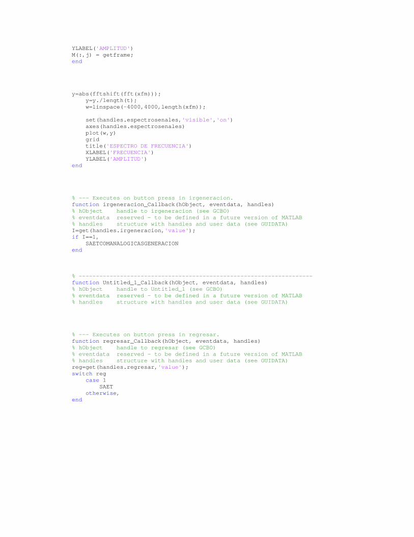
YLABEL('AMPLITUD') M(:,j) = getframe; end y=abs(fftshift(fft(xfm))); y=y./length(t); w=linspace(-4000,4000,length(xfm)); set(handles.espectrosenales,'visible','on') axes(handles.espectrosenales) plot(w,y) grid title('ESPECTRO DE FRECUENCIA') XLABEL('FRECUENCIA') YLABEL('AMPLITUD') end % --- Executes on button press in irgeneracion. function irgeneracion_Callback(hObject, eventdata, handles) % hObject handle to irgeneracion (see GCBO) % eventdata reserved - to be defined in a future version of MATLAB % handles structure with handles and user data (see GUIDATA) I=get(handles.irgeneracion,'value'); if I==1, SAETCOMANALOGICASGENERACION end % -------------------------------------------------------------------- function Untitled_1_Callback(hObject, eventdata, handles) % hObject handle to Untitled_1 (see GCBO) % eventdata reserved - to be defined in a future version of MATLAB % handles structure with handles and user data (see GUIDATA) % --- Executes on button press in regresar. function regresar_Callback(hObject, eventdata, handles) % hObject handle to regresar (see GCBO) % eventdata reserved - to be defined in a future version of MATLAB % handles structure with handles and user data (see GUIDATA) reg=get(handles.regresar,'value'); switch reg case 1 SAET otherwise, end
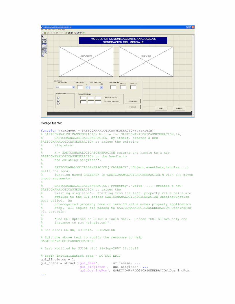
Codigo fuente: function varargout = SAETCOMANALOGICASGENERACION(varargin) % SAETCOMANALOGICASGENERACION M-file for SAETCOMANALOGICASGENERACION.fig % SAETCOMANALOGICASGENERACION, by itself, creates a new SAETCOMANALOGICASGENERACION or raises the existing % singleton*. % % H = SAETCOMANALOGICASGENERACION returns the handle to a new SAETCOMANALOGICASGENERACION or the handle to % the existing singleton*. % % SAETCOMANALOGICASGENERACION('CALLBACK',hObject,eventData,handles,...) calls the local % function named CALLBACK in SAETCOMANALOGICASGENERACION.M with the given input arguments. % % SAETCOMANALOGICASGENERACION('Property','Value',...) creates a new SAETCOMANALOGICASGENERACION or raises the % existing singleton*. Starting from the left, property value pairs are % applied to the GUI before SAETCOMANALOGICASGENERACION_OpeningFunction gets called. An % unrecognized property name or invalid value makes property application % stop. All inputs are passed to SAETCOMANALOGICASGENERACION_OpeningFcn via varargin. % % *See GUI Options on GUIDE's Tools menu. Choose "GUI allows only one % instance to run (singleton)". % % See also: GUIDE, GUIDATA, GUIHANDLES % Edit the above text to modify the response to help SAETCOMANALOGICASGENERACION % Last Modified by GUIDE v2.5 28-Sep-2007 12:33:14 % Begin initialization code - DO NOT EDIT gui_Singleton = 1; gui_State = struct('gui_Name', mfilename, ... 'gui_Singleton', gui_Singleton, ... 'gui_OpeningFcn', @SAETCOMANALOGICASGENERACION_OpeningFcn, ...

'gui_OutputFcn', @SAETCOMANALOGICASGENERACION_OutputFcn, ... 'gui_LayoutFcn', [] , ... 'gui_Callback', []); if nargin && ischar(varargin{1}) gui_State.gui_Callback = str2func(varargin{1}); end if nargout [varargout{1:nargout}] = gui_mainfcn(gui_State, varargin{:}); else gui_mainfcn(gui_State, varargin{:}); end % End initialization code - DO NOT EDIT % --- Executes just before SAETCOMANALOGICASGENERACION is made visible. function SAETCOMANALOGICASGENERACION_OpeningFcn(hObject, eventdata, handles, varargin) % This function has no output args, see OutputFcn. % hObject handle to figure % eventdata reserved - to be defined in a future version of MATLAB % handles structure with handles and user data (see GUIDATA) % varargin command line arguments to SAETCOMANALOGICASGENERACION (see VARARGIN) % Choose default command line output for SAETCOMANALOGICASGENERACION handles.output = hObject; % Update handles structure guidata(hObject, handles); % UIWAIT makes SAETCOMANALOGICASGENERACION wait for user response (see UIRESUME) % uiwait(handles.figure1); % --- Outputs from this function are returned to the command line. function varargout = SAETCOMANALOGICASGENERACION_OutputFcn(hObject, eventdata, handles) % varargout cell array for returning output args (see VARARGOUT); % hObject handle to figure % eventdata reserved - to be defined in a future version of MATLAB % handles structure with handles and user data (see GUIDATA) % Get default command line output from handles structure varargout{1} = handles.output; % --- Executes on selection change in ANALOGICOESCOGER. function ANALOGICOESCOGER_Callback(hObject, eventdata, handles) % hObject handle to ANALOGICOESCOGER (see GCBO) % eventdata reserved - to be defined in a future version of MATLAB % handles structure with handles and user data (see GUIDATA) % Hints: contents = get(hObject,'String') returns ANALOGICOESCOGER contents as cell array % contents{get(hObject,'Value')} returns selected item from ANALOGICOESCOGER % --- Executes during object creation, after setting all properties. function ANALOGICOESCOGER_CreateFcn(hObject, eventdata, handles) % hObject handle to ANALOGICOESCOGER (see GCBO) % eventdata reserved - to be defined in a future version of MATLAB % handles empty - handles not created until after all CreateFcns called % Hint: popupmenu controls usually have a white background on Windows.

% See ISPC and COMPUTER. if ispc && isequal(get(hObject,'BackgroundColor'), get(0,'defaultUicontrolBackgroundColor')) set(hObject,'BackgroundColor','white'); end % --- Executes on button press in ANALOGICOPROCESAR. function ANALOGICOPROCESAR_Callback(hObject, eventdata, handles) % hObject handle to ANALOGICOPROCESAR (see GCBO) % eventdata reserved - to be defined in a future version of MATLAB % handles structure with handles and user data (see GUIDATA) p=get(handles.ANALOGICOPROCESAR,'value'); if p==1, b=get(handles.ANALOGICOESCOGER,'value'); switch b case 1 %onda seno set(handles.PARAMETROSTONOS,'visible','on') set(handles.NUMTONOS,'visible','on') global Fc; global amplitud; global t; M = moviein(50); t=1/8000:1/8000:2; for j=1:50, Fc=get(handles.ANALOGICOFRECUENCIA,'value'); Fc=Fc*1000; amplitud=str2double(get(handles.ANALOGICOAMPLITUD,'String')); %validacion if isnan(amplitud) beep set(handles.ANALOGICOAMPLITUD,'String',0); amplitud=0; errordlg('El valor debe ser numérico','ERROR') end x=amplitud*sin(2*(pi/4)*Fc*(t+j)); set(handles.SENALTIEMPO,'visible','on') axes(handles.SENALTIEMPO) plot(t,x); grid AXIS([0 0.02 min(x) max(x)]) title('DOMINIO DEL TIEMPO') XLABEL('TIEMPO') YLABEL('AMPLITUD') M(:,j) = getframe; end cla global amplitud; global t; set(handles.ANALOGICOFRECUENCIA1,'string',Fc) offset=str2double(get(handles.ANALOGICOOFFSET,'String')); %validacion if isnan(offset) beep set(handles.ANALOGICOOFFSET,'String',0); offset=0; errordlg('El valor debe ser numérico','ERROR') end fase=str2double(get(handles.ANALOGICOFASE,'String')); %validacion if isnan(fase)

beep set(handles.ANALOGICOFASE,'String',0); fase=0; errordlg('El valor debe ser numérico','ERROR') end %creo la forma de onda mensaje=amplitud*sin((2*pi*Fc*t)+fase); mensaje=mensaje+offset; save datos2.mat mensaje set(handles.SENALTIEMPO,'visible','on') axes(handles.SENALTIEMPO) plot(mensaje) grid AXIS([0 200 min(mensaje) max(mensaje)]) title('DOMINIO DEL TIEMPO') XLABEL('TIEMPO') YLABEL('AMPLITUD') %ESPECTRO EN FRECUENCIA y=abs(fftshift(fft(mensaje))); y=y./length(t); w=linspace(-4000,4000,length(mensaje)); set(handles.SENALFREC,'visible','on') axes(handles.SENALFREC) plot(w,y) grid title('ESPECTRO DE FRECUENCIA') XLABEL('FRECUENCIA') YLABEL('AMPLITUD') case 2 %onda coseno set(handles.PARAMETROSTONOS,'visible','on') set(handles.NUMTONOS,'visible','on') global Fc; global amplitud; global t; M = moviein(50); t=1/8000:1/8000:2; for j=1:50, Fc=get(handles.ANALOGICOFRECUENCIA,'value'); Fc=Fc*1000; amplitud=str2double(get(handles.ANALOGICOAMPLITUD,'String')); %validacion if isnan(amplitud) beep set(handles.ANALOGICOAMPLITUD,'String',0); amplitud=0; errordlg('El valor debe ser numérico','ERROR') end x=amplitud*cos(2*(pi/4)*Fc*(t+j)); set(handles.SENALTIEMPO,'visible','on') axes(handles.SENALTIEMPO) plot(t,x,'r'); grid AXIS([0 0.02 min(x) max(x)]) title('DOMINIO DEL TIEMPO') XLABEL('TIEMPO') YLABEL('AMPLITUD') M(:,j) = getframe; end cla global amplitud; global t; set(handles.ANALOGICOFRECUENCIA1,'string',Fc) offset=str2double(get(handles.ANALOGICOOFFSET,'String'));
%validacion if isnan(offset) beep set(handles.ANALOGICOOFFSET,'String',0); offset=0; errordlg('El valor debe ser numérico','ERROR') end fase=str2double(get(handles.ANALOGICOFASE,'String')); %validacion if isnan(fase) beep set(handles.ANALOGICOFASE,'String',0); fase=0; errordlg('El valor debe ser numérico','ERROR') end %creo la forma de onda mensaje=amplitud*cos((2*pi*Fc*t)+fase); mensaje=mensaje+offset; save datos2.mat mensaje set(handles.SENALTIEMPO,'visible','on') axes(handles.SENALTIEMPO) plot(mensaje,'r') grid AXIS([0 200 min(mensaje) max(mensaje)]) title('DOMINIO DEL TIEMPO') XLABEL('TIEMPO') YLABEL('AMPLITUD') %ESPECTRO EN FRECUENCIA y=abs(fftshift(fft(mensaje))); y=y./length(t); w=linspace(-4000,4000,length(mensaje)); set(handles.SENALFREC,'visible','on') axes(handles.SENALFREC) plot(w,y) grid title('ESPECTRO DE FRECUENCIA') XLABEL('FRECUENCIA') YLABEL('AMPLITUD') case 3 %multitono seno set(handles.PARAMETROSTONOS,'visible','on') set(handles.NUMTONOS,'visible','on') global Fc; global amplitud; global t; Fc=get(handles.ANALOGICOFRECUENCIA,'value'); Fc=Fc*1000; amplitud=str2double(get(handles.ANALOGICOAMPLITUD,'String')); %validacion if isnan(amplitud) beep set(handles.ANALOGICOAMPLITUD,'String',0); amplitud=0; errordlg('El valor debe ser numérico','ERROR') end offset=str2double(get(handles.ANALOGICOOFFSET,'String')); %validacion if isnan(offset) beep set(handles.ANALOGICOOFFSET,'String',0);

offset=0; errordlg('El valor debe ser numérico','ERROR') end fase=str2double(get(handles.ANALOGICOFASE,'String')); %validacion if isnan(fase) beep set(handles.ANALOGICOFASE,'String',0); fase=0; errordlg('El valor debe ser numérico','ERROR') end set(handles.ANALOGICOFRECUENCIA1,'string',Fc) numtonos=get(handles.NUMERODETONOS,'value'); numtonos2=get(handles.NUMERODETONOS2,'value'); numtonos3=get(handles.NUMERODETONOS3,'value'); if numtonos==1, set(handles.A3,'visible','off') set(handles.F3,'visible','off') set(handles.A4,'visible','off') set(handles.F4,'visible','off') M = moviein(50); t=1/8000:1/8000:2; for j=1:50, A2=str2double(get(handles.A2,'String')); if isnan(A2) beep set(handles.A2,'String',0); A2=0; errordlg('El valor debe ser numérico','ERROR') end F2=str2double(get(handles.F2,'String')); if isnan(F2) beep set(handles.F2,'String',0); F2=0; errordlg('El valor debe ser numérico','ERROR') end x1=amplitud*(0.75)*sin(2*(pi/4)*Fc*(t+j))+A2*(0.5)*sin(2*(pi/4)*F2*(t+j)); set(handles.SENALTIEMPO,'visible','on') axes(handles.SENALTIEMPO) plot(t,x1); grid AXIS([0 0.02 min(x1) max(x1)]) title('DOMINIO DEL TIEMPO') XLABEL('TIEMPO') YLABEL('AMPLITUD') M(:,j) = getframe; end %creo la forma de onda mensaje1=amplitud*sin((2*pi*Fc*t)+fase)+A2*sin((2*pi*F2*t)+fase); mensaje1=mensaje1+offset; mensaje=mensaje1; save datos2.mat mensaje set(handles.SENALTIEMPO,'visible','on') axes(handles.SENALTIEMPO) plot(mensaje1) grid AXIS([0 200 min(mensaje1) max(mensaje1)]) title('DOMINIO DEL TIEMPO') XLABEL('TIEMPO') YLABEL('AMPLITUD') %ESPECTRO EN FRECUENCIA y=abs(fftshift(fft(mensaje1)));

y=y./length(mensaje1); w=linspace(-4000,4000,length(mensaje1)); set(handles.SENALFREC,'visible','on') axes(handles.SENALFREC) plot(w,y) grid title('ESPECTRO DE FRECUENCIA') XLABEL('FRECUENCIA') YLABEL('AMPLITUD') end if numtonos2==1, set(handles.A4,'visible','off') set(handles.F4,'visible','off') set(handles.A3,'visible','on') set(handles.F3,'visible','on') M = moviein(50); t=1/8000:1/8000:2; for j=1:50, A2=str2double(get(handles.A2,'String')); if isnan(A2) beep set(handles.A2,'String',0); A2=0; errordlg('El valor debe ser numérico','ERROR') end F2=str2double(get(handles.F2,'String')); if isnan(F2) beep set(handles.F2,'String',0); F2=0; errordlg('El valor debe ser numérico','ERROR') end A3=str2double(get(handles.A3,'String')); if isnan(A3) beep set(handles.A3,'String',0); A3=0; errordlg('El valor debe ser numérico','ERROR') end F3=str2double(get(handles.F3,'String')); if isnan(F3) beep set(handles.F3,'String',0); F3=0; errordlg('El valor debe ser numérico','ERROR') end x2=amplitud*(0.75)*sin(2*(pi/4)*Fc*(t+j))+A2*(0.5)*sin(2*(pi/4)*F2*(t+j))+A3*(0.5)*sin(2*(pi/4)*F3*(t+j)); set(handles.SENALTIEMPO,'visible','on') axes(handles.SENALTIEMPO) plot(t,x2); grid AXIS([0 0.02 min(x2) max(x2)]) title('DOMINIO DEL TIEMPO') XLABEL('TIEMPO') YLABEL('AMPLITUD') M(:,j) = getframe; end %creo la forma de onda mensaje2=amplitud*sin((2*pi*Fc*t)+fase)+A2*sin((2*pi*F2*t)+fase)+A3*sin((2*pi*F3*t)+fase); mensaje2=mensaje2+offset; mensaje=mensaje2; save datos2.mat mensaje set(handles.SENALTIEMPO,'visible','on') axes(handles.SENALTIEMPO)

plot(mensaje2) grid AXIS([0 200 min(mensaje2) max(mensaje2)]) title('DOMINIO DEL TIEMPO') XLABEL('TIEMPO') YLABEL('AMPLITUD') %ESPECTRO EN FRECUENCIA y=abs(fftshift(fft(mensaje2))); y=y./length(mensaje2); w=linspace(-4000,4000,length(mensaje2)); set(handles.SENALFREC,'visible','on') axes(handles.SENALFREC) plot(w,y) grid title('ESPECTRO DE FRECUENCIA') XLABEL('FRECUENCIA') YLABEL('AMPLITUD') end if numtonos3==1, set(handles.A4,'visible','on') set(handles.F4,'visible','on') set(handles.A3,'visible','on') set(handles.F3,'visible','on') M = moviein(50); t=1/8000:1/8000:2; for j=1:50, A2=str2double(get(handles.A2,'String')); if isnan(A2) beep set(handles.A2,'String',0); A2=0; errordlg('El valor debe ser numérico','ERROR') end F2=str2double(get(handles.F2,'String')); if isnan(F2) beep set(handles.F2,'String',0); F2=0; errordlg('El valor debe ser numérico','ERROR') end A3=str2double(get(handles.A3,'String')); if isnan(A3) beep set(handles.A3,'String',0); A3=0; errordlg('El valor debe ser numérico','ERROR') end F3=str2double(get(handles.F3,'String')); if isnan(F3) beep set(handles.F3,'String',0); F3=0; errordlg('El valor debe ser numérico','ERROR') end A4=str2double(get(handles.A4,'String')); if isnan(A4) beep set(handles.A4,'String',0); A4=0; errordlg('El valor debe ser numérico','ERROR') end F4=str2double(get(handles.F4,'String')); if isnan(F4) beep set(handles.F4,'String',0); F4=0; errordlg('El valor debe ser numérico','ERROR') end

x3=amplitud*(0.75)*sin(2*(pi/4)*Fc*(t+j))+A2*(0.5)*sin(2*(pi/4)*F2*(t+j))+A3*(0.5)*sin(2*(pi/4)*F3*(t+j))+A4*(0.5)*sin(2*(pi/4)*F4*(t+j)); set(handles.SENALTIEMPO,'visible','on') axes(handles.SENALTIEMPO) plot(t,x3); grid AXIS([0 0.02 min(x3) max(x3)]) title('DOMINIO DEL TIEMPO') XLABEL('TIEMPO') YLABEL('AMPLITUD') M(:,j) = getframe; end %creo la forma de onda mensaje3=amplitud*sin((2*pi*Fc*t)+fase)+A2*sin((2*pi*F2*t)+fase)+A3*sin((2*pi*F3*t)+fase)+A4*sin((2*pi*F4*t)+fase); mensaje3=mensaje3+offset; mensaje=mensaje3; save datos2.mat mensaje set(handles.SENALTIEMPO,'visible','on') axes(handles.SENALTIEMPO) plot(mensaje3) grid AXIS([0 200 min(mensaje3) max(mensaje3)]) title('DOMINIO DEL TIEMPO') XLABEL('TIEMPO') YLABEL('AMPLITUD') %ESPECTRO EN FRECUENCIA y=abs(fftshift(fft(mensaje3))); y=y./length(mensaje3); w=linspace(-4000,4000,length(mensaje3)); set(handles.SENALFREC,'visible','on') axes(handles.SENALFREC) plot(w,y) grid title('ESPECTRO DE FRECUENCIA') XLABEL('FRECUENCIA') YLABEL('AMPLITUD') end case 4 %multitono coseno set(handles.PARAMETROSTONOS,'visible','on') set(handles.NUMTONOS,'visible','on') global Fc; global amplitud; global t; Fc=get(handles.ANALOGICOFRECUENCIA,'value'); Fc=Fc*1000; amplitud=str2double(get(handles.ANALOGICOAMPLITUD,'String')); %validacion if isnan(amplitud) beep set(handles.ANALOGICOAMPLITUD,'String',0); amplitud=0; errordlg('El valor debe ser numérico','ERROR') end offset=str2double(get(handles.ANALOGICOOFFSET,'String')); %validacion if isnan(offset) beep set(handles.ANALOGICOOFFSET,'String',0); offset=0; errordlg('El valor debe ser numérico','ERROR') end

fase=str2double(get(handles.ANALOGICOFASE,'String')); %validacion if isnan(fase) beep set(handles.ANALOGICOFASE,'String',0); fase=0; errordlg('El valor debe ser numérico','ERROR') end set(handles.ANALOGICOFRECUENCIA1,'string',Fc) numtonos=get(handles.NUMERODETONOS,'value'); numtonos2=get(handles.NUMERODETONOS2,'value'); numtonos3=get(handles.NUMERODETONOS3,'value'); load datos2.mat if numtonos==1, set(handles.A3,'visible','off') set(handles.F3,'visible','off') set(handles.A4,'visible','off') set(handles.F4,'visible','off') M = moviein(50); t=1/8000:1/8000:2; for j=1:50, A2=str2double(get(handles.A2,'String')); if isnan(A2) beep set(handles.A2,'String',0); A2=0; errordlg('El valor debe ser numérico','ERROR') end F2=str2double(get(handles.F2,'String')); if isnan(F2) beep set(handles.F2,'String',0); F2=0; errordlg('El valor debe ser numérico','ERROR') end x1=amplitud*(0.75)*cos(2*(pi/4)*Fc*(t+j))+A2*(0.5)*cos(2*(pi/4)*F2*(t+j)); set(handles.SENALTIEMPO,'visible','on') axes(handles.SENALTIEMPO) plot(t,x1); grid AXIS([0 0.02 min(x1) max(x1)]) title('DOMINIO DEL TIEMPO') XLABEL('TIEMPO') YLABEL('AMPLITUD') M(:,j) = getframe; end %creo la forma de onda mensaje1=amplitud*cos((2*pi*Fc*t)+fase)+A2*cos((2*pi*F2*t)+fase); mensaje1=mensaje1+offset; mensaje=mensaje1; save datos2.mat mensaje set(handles.SENALTIEMPO,'visible','on') axes(handles.SENALTIEMPO) plot(mensaje1) grid AXIS([0 200 min(mensaje1) max(mensaje1)]) title('DOMINIO DEL TIEMPO') XLABEL('TIEMPO') YLABEL('AMPLITUD') %ESPECTRO EN FRECUENCIA y=abs(fftshift(fft(mensaje1))); y=y./length(mensaje1); w=linspace(-4000,4000,length(mensaje1));

set(handles.SENALFREC,'visible','on') axes(handles.SENALFREC) plot(w,y) grid title('ESPECTRO DE FRECUENCIA') XLABEL('FRECUENCIA') YLABEL('AMPLITUD') end if numtonos2==1, set(handles.A4,'visible','off') set(handles.F4,'visible','off') set(handles.A3,'visible','on') set(handles.F3,'visible','on') M = moviein(50); t=1/8000:1/8000:2; for j=1:50, A2=str2double(get(handles.A2,'String')); if isnan(A2) beep set(handles.A2,'String',0); A2=0; errordlg('El valor debe ser numérico','ERROR') end F2=str2double(get(handles.F2,'String')); if isnan(F2) beep set(handles.F2,'String',0); F2=0; errordlg('El valor debe ser numérico','ERROR') end A3=str2double(get(handles.A3,'String')); if isnan(A3) beep set(handles.A3,'String',0); A3=0; errordlg('El valor debe ser numérico','ERROR') end F3=str2double(get(handles.F3,'String')); if isnan(F3) beep set(handles.F3,'String',0); F3=0; errordlg('El valor debe ser numérico','ERROR') end x2=amplitud*(0.75)*cos(2*(pi/4)*Fc*(t+j))+A2*(0.5)*cos(2*(pi/4)*F2*(t+j))+A3*(0.5)*cos(2*(pi/4)*F3*(t+j)); set(handles.SENALTIEMPO,'visible','on') axes(handles.SENALTIEMPO) plot(t,x2); grid AXIS([0 0.02 min(x2) max(x2)]) title('DOMINIO DEL TIEMPO') XLABEL('TIEMPO') YLABEL('AMPLITUD') M(:,j) = getframe; end %creo la forma de onda mensaje2=amplitud*cos((2*pi*Fc*t)+fase)+A2*cos((2*pi*F2*t)+fase)+A3*cos((2*pi*F3*t)+fase); mensaje2=mensaje2+offset; mensaje=mensaje2; save datos2.mat mensaje set(handles.SENALTIEMPO,'visible','on') axes(handles.SENALTIEMPO)
plot(mensaje2) grid AXIS([0 200 min(mensaje2) max(mensaje2)]) title('DOMINIO DEL TIEMPO') XLABEL('TIEMPO') YLABEL('AMPLITUD') %ESPECTRO EN FRECUENCIA y=abs(fftshift(fft(mensaje2))); y=y./length(mensaje2); w=linspace(-4000,4000,length(mensaje2)); set(handles.SENALFREC,'visible','on') axes(handles.SENALFREC) plot(w,y) grid title('ESPECTRO DE FRECUENCIA') XLABEL('FRECUENCIA') YLABEL('AMPLITUD') end if numtonos3==1, set(handles.A4,'visible','on') set(handles.F4,'visible','on') set(handles.A3,'visible','on') set(handles.F3,'visible','on') M = moviein(50); t=1/8000:1/8000:2; for j=1:50, A2=str2double(get(handles.A2,'String')); if isnan(A2) beep set(handles.A2,'String',0); A2=0; errordlg('El valor debe ser numérico','ERROR') end F2=str2double(get(handles.F2,'String')); if isnan(F2) beep set(handles.F2,'String',0); F2=0; errordlg('El valor debe ser numérico','ERROR') end A3=str2double(get(handles.A3,'String')); if isnan(A3) beep set(handles.A3,'String',0); A3=0; errordlg('El valor debe ser numérico','ERROR') end F3=str2double(get(handles.F3,'String')); if isnan(F3) beep set(handles.F3,'String',0); F3=0; errordlg('El valor debe ser numérico','ERROR') end A4=str2double(get(handles.A4,'String')); if isnan(A4) beep set(handles.A4,'String',0); A4=0; errordlg('El valor debe ser numérico','ERROR') end F4=str2double(get(handles.F4,'String')); if isnan(F4) beep set(handles.F4,'String',0); F4=0; errordlg('El valor debe ser numérico','ERROR') end

x3=amplitud*(0.75)*cos(2*(pi/4)*Fc*(t+j))+A2*(0.5)*cos(2*(pi/4)*F2*(t+j))+A3*(0.5)*cos(2*(pi/4)*F3*(t+j))+A4*(0.5)*cos(2*(pi/4)*F4*(t+j)); set(handles.SENALTIEMPO,'visible','on') axes(handles.SENALTIEMPO) plot(t,x3); grid AXIS([0 0.02 min(x3) max(x3)]) title('DOMINIO DEL TIEMPO') XLABEL('TIEMPO') YLABEL('AMPLITUD') M(:,j) = getframe; end %creo la forma de onda mensaje3=amplitud*cos((2*pi*Fc*t)+fase)+A2*cos((2*pi*F2*t)+fase)+A3*cos((2*pi*F3*t)+fase)+A4*cos((2*pi*F4*t)+fase); mensaje3=mensaje3+offset; mensaje=mensaje3; save datos2.mat mensaje set(handles.SENALTIEMPO,'visible','on') axes(handles.SENALTIEMPO) plot(mensaje3) grid AXIS([0 200 min(mensaje3) max(mensaje3)]) title('DOMINIO DEL TIEMPO') XLABEL('TIEMPO') YLABEL('AMPLITUD') %ESPECTRO EN FRECUENCIA y=abs(fftshift(fft(mensaje3))); y=y./length(mensaje3); w=linspace(-4000,4000,length(mensaje3)); set(handles.SENALFREC,'visible','on') axes(handles.SENALFREC) plot(w,y) grid title('ESPECTRO DE FRECUENCIA') XLABEL('FRECUENCIA') YLABEL('AMPLITUD') end case 5 %voz % set(handles.A2,'visible','off') % set(handles.F2,'visible','off') % set(handles.A3,'visible','off') % set(handles.F3,'visible','off') % set(handles.A4,'visible','off') % set(handles.F4,'visible','off') set(handles.PARAMETROSTONOS,'visible','off') set(handles.NUMTONOS,'visible','off') % set(handles.FASE11,'visible','off') % set(handles.CICLODETRABAJO11,'visible','off') % set(handles.CICLODETRABAJO1,'visible','off') % %G=get(handles.GRABAR1,'value'); Fs = 11025*2; voz = wavrecord(16000, Fs); %cinco seg de grabacion mensaje=voz; global t; %formadeonda1=formadeonda1(1:16000); mensaje=mensaje'; save datos2.mat mensaje wavplay(voz, Fs); set(handles.SENALTIEMPO,'visible','on') axes(handles.SENALTIEMPO) plot(voz) grid

title('DOMINIO TIEMPO') XLABEL('TIEMPO') YLABEL('AMPLITUD') %ESPECTRO EN FRECUENCIA y=abs(fftshift(fft(voz))); y=y./length(voz); w=linspace(-Fs/2,Fs/2,length(voz)); set(handles.SENALFREC,'visible','on') axes(handles.SENALFREC) plot(w,y) grid title('ESPECTRO DE FRECUENCIA') XLABEL('FRECUENCIA') YLABEL('AMPLITUD') otherwise, end end function ANALOGICOAMPLITUD_Callback(hObject, eventdata, handles) % hObject handle to ANALOGICOAMPLITUD (see GCBO) % eventdata reserved - to be defined in a future version of MATLAB % handles structure with handles and user data (see GUIDATA) % Hints: get(hObject,'String') returns contents of ANALOGICOAMPLITUD as text % str2double(get(hObject,'String')) returns contents of ANALOGICOAMPLITUD as a double % --- Executes during object creation, after setting all properties. function ANALOGICOAMPLITUD_CreateFcn(hObject, eventdata, handles) % hObject handle to ANALOGICOAMPLITUD (see GCBO) % eventdata reserved - to be defined in a future version of MATLAB % handles empty - handles not created until after all CreateFcns called % Hint: edit controls usually have a white background on Windows. % See ISPC and COMPUTER. if ispc && isequal(get(hObject,'BackgroundColor'), get(0,'defaultUicontrolBackgroundColor')) set(hObject,'BackgroundColor','white'); end % --- Executes on slider movement. function ANALOGICOFRECUENCIA_Callback(hObject, eventdata, handles) % hObject handle to ANALOGICOFRECUENCIA (see GCBO) % eventdata reserved - to be defined in a future version of MATLAB % handles structure with handles and user data (see GUIDATA) % Hints: get(hObject,'Value') returns position of slider % get(hObject,'Min') and get(hObject,'Max') to determine range of slider % --- Executes during object creation, after setting all properties. function ANALOGICOFRECUENCIA_CreateFcn(hObject, eventdata, handles) % hObject handle to ANALOGICOFRECUENCIA (see GCBO) % eventdata reserved - to be defined in a future version of MATLAB % handles empty - handles not created until after all CreateFcns called % Hint: slider controls usually have a light gray background. if isequal(get(hObject,'BackgroundColor'), get(0,'defaultUicontrolBackgroundColor'))

set(hObject,'BackgroundColor',[.9 .9 .9]); end function ANALOGICOFRECUENCIA1_Callback(hObject, eventdata, handles) % hObject handle to ANALOGICOFRECUENCIA1 (see GCBO) % eventdata reserved - to be defined in a future version of MATLAB % handles structure with handles and user data (see GUIDATA) % Hints: get(hObject,'String') returns contents of ANALOGICOFRECUENCIA1 as text % str2double(get(hObject,'String')) returns contents of ANALOGICOFRECUENCIA1 as a double % --- Executes during object creation, after setting all properties. function ANALOGICOFRECUENCIA1_CreateFcn(hObject, eventdata, handles) % hObject handle to ANALOGICOFRECUENCIA1 (see GCBO) % eventdata reserved - to be defined in a future version of MATLAB % handles empty - handles not created until after all CreateFcns called % Hint: edit controls usually have a white background on Windows. % See ISPC and COMPUTER. if ispc && isequal(get(hObject,'BackgroundColor'), get(0,'defaultUicontrolBackgroundColor')) set(hObject,'BackgroundColor','white'); end % --- Executes on button press in NUMERODETONOS. function NUMERODETONOS_Callback(hObject, eventdata, handles) % hObject handle to NUMERODETONOS (see GCBO) % eventdata reserved - to be defined in a future version of MATLAB % handles structure with handles and user data (see GUIDATA) % Hint: get(hObject,'Value') returns toggle state of NUMERODETONOS % --- Executes on button press in NUMERODETONOS2. function NUMERODETONOS2_Callback(hObject, eventdata, handles) % hObject handle to NUMERODETONOS2 (see GCBO) % eventdata reserved - to be defined in a future version of MATLAB % handles structure with handles and user data (see GUIDATA) % Hint: get(hObject,'Value') returns toggle state of NUMERODETONOS2 % --- Executes on button press in NUMERODETONOS3. function NUMERODETONOS3_Callback(hObject, eventdata, handles) % hObject handle to NUMERODETONOS3 (see GCBO) % eventdata reserved - to be defined in a future version of MATLAB % handles structure with handles and user data (see GUIDATA) % Hint: get(hObject,'Value') returns toggle state of NUMERODETONOS3 function A2_Callback(hObject, eventdata, handles) % hObject handle to A2 (see GCBO) % eventdata reserved - to be defined in a future version of MATLAB % handles structure with handles and user data (see GUIDATA) % Hints: get(hObject,'String') returns contents of A2 as text % str2double(get(hObject,'String')) returns contents of A2 as a double % --- Executes during object creation, after setting all properties.

function A2_CreateFcn(hObject, eventdata, handles) % hObject handle to A2 (see GCBO) % eventdata reserved - to be defined in a future version of MATLAB % handles empty - handles not created until after all CreateFcns called % Hint: edit controls usually have a white background on Windows. % See ISPC and COMPUTER. if ispc && isequal(get(hObject,'BackgroundColor'), get(0,'defaultUicontrolBackgroundColor')) set(hObject,'BackgroundColor','white'); end function A3_Callback(hObject, eventdata, handles) % hObject handle to A3 (see GCBO) % eventdata reserved - to be defined in a future version of MATLAB % handles structure with handles and user data (see GUIDATA) % Hints: get(hObject,'String') returns contents of A3 as text % str2double(get(hObject,'String')) returns contents of A3 as a double % --- Executes during object creation, after setting all properties. function A3_CreateFcn(hObject, eventdata, handles) % hObject handle to A3 (see GCBO) % eventdata reserved - to be defined in a future version of MATLAB % handles empty - handles not created until after all CreateFcns called % Hint: edit controls usually have a white background on Windows. % See ISPC and COMPUTER. if ispc && isequal(get(hObject,'BackgroundColor'), get(0,'defaultUicontrolBackgroundColor')) set(hObject,'BackgroundColor','white'); end function A4_Callback(hObject, eventdata, handles) % hObject handle to A4 (see GCBO) % eventdata reserved - to be defined in a future version of MATLAB % handles structure with handles and user data (see GUIDATA) % Hints: get(hObject,'String') returns contents of A4 as text % str2double(get(hObject,'String')) returns contents of A4 as a double % --- Executes during object creation, after setting all properties. function A4_CreateFcn(hObject, eventdata, handles) % hObject handle to A4 (see GCBO) % eventdata reserved - to be defined in a future version of MATLAB % handles empty - handles not created until after all CreateFcns called % Hint: edit controls usually have a white background on Windows. % See ISPC and COMPUTER. if ispc && isequal(get(hObject,'BackgroundColor'), get(0,'defaultUicontrolBackgroundColor')) set(hObject,'BackgroundColor','white'); end function F2_Callback(hObject, eventdata, handles) % hObject handle to F2 (see GCBO) % eventdata reserved - to be defined in a future version of MATLAB % handles structure with handles and user data (see GUIDATA) % Hints: get(hObject,'String') returns contents of F2 as text

% str2double(get(hObject,'String')) returns contents of F2 as a double % --- Executes during object creation, after setting all properties. function F2_CreateFcn(hObject, eventdata, handles) % hObject handle to F2 (see GCBO) % eventdata reserved - to be defined in a future version of MATLAB % handles empty - handles not created until after all CreateFcns called % Hint: edit controls usually have a white background on Windows. % See ISPC and COMPUTER. if ispc && isequal(get(hObject,'BackgroundColor'), get(0,'defaultUicontrolBackgroundColor')) set(hObject,'BackgroundColor','white'); end function F3_Callback(hObject, eventdata, handles) % hObject handle to F3 (see GCBO) % eventdata reserved - to be defined in a future version of MATLAB % handles structure with handles and user data (see GUIDATA) % Hints: get(hObject,'String') returns contents of F3 as text % str2double(get(hObject,'String')) returns contents of F3 as a double % --- Executes during object creation, after setting all properties. function F3_CreateFcn(hObject, eventdata, handles) % hObject handle to F3 (see GCBO) % eventdata reserved - to be defined in a future version of MATLAB % handles empty - handles not created until after all CreateFcns called % Hint: edit controls usually have a white background on Windows. % See ISPC and COMPUTER. if ispc && isequal(get(hObject,'BackgroundColor'), get(0,'defaultUicontrolBackgroundColor')) set(hObject,'BackgroundColor','white'); end function F4_Callback(hObject, eventdata, handles) % hObject handle to F4 (see GCBO) % eventdata reserved - to be defined in a future version of MATLAB % handles structure with handles and user data (see GUIDATA) % Hints: get(hObject,'String') returns contents of F4 as text % str2double(get(hObject,'String')) returns contents of F4 as a double % --- Executes during object creation, after setting all properties. function F4_CreateFcn(hObject, eventdata, handles) % hObject handle to F4 (see GCBO) % eventdata reserved - to be defined in a future version of MATLAB % handles empty - handles not created until after all CreateFcns called % Hint: edit controls usually have a white background on Windows. % See ISPC and COMPUTER. if ispc && isequal(get(hObject,'BackgroundColor'), get(0,'defaultUicontrolBackgroundColor')) set(hObject,'BackgroundColor','white'); end function ANALOGICOFASE_Callback(hObject, eventdata, handles) % hObject handle to ANALOGICOFASE (see GCBO)

% eventdata reserved - to be defined in a future version of MATLAB % handles structure with handles and user data (see GUIDATA) % Hints: get(hObject,'String') returns contents of ANALOGICOFASE as text % str2double(get(hObject,'String')) returns contents of ANALOGICOFASE as a double % --- Executes during object creation, after setting all properties. function ANALOGICOFASE_CreateFcn(hObject, eventdata, handles) % hObject handle to ANALOGICOFASE (see GCBO) % eventdata reserved - to be defined in a future version of MATLAB % handles empty - handles not created until after all CreateFcns called % Hint: edit controls usually have a white background on Windows. % See ISPC and COMPUTER. if ispc && isequal(get(hObject,'BackgroundColor'), get(0,'defaultUicontrolBackgroundColor')) set(hObject,'BackgroundColor','white'); end function ANALOGICOOFFSET_Callback(hObject, eventdata, handles) % hObject handle to ANALOGICOOFFSET (see GCBO) % eventdata reserved - to be defined in a future version of MATLAB % handles structure with handles and user data (see GUIDATA) % Hints: get(hObject,'String') returns contents of ANALOGICOOFFSET as text % str2double(get(hObject,'String')) returns contents of ANALOGICOOFFSET as a double % --- Executes during object creation, after setting all properties. function ANALOGICOOFFSET_CreateFcn(hObject, eventdata, handles) % hObject handle to ANALOGICOOFFSET (see GCBO) % eventdata reserved - to be defined in a future version of MATLAB % handles empty - handles not created until after all CreateFcns called % Hint: edit controls usually have a white background on Windows. % See ISPC and COMPUTER. if ispc && isequal(get(hObject,'BackgroundColor'), get(0,'defaultUicontrolBackgroundColor')) set(hObject,'BackgroundColor','white'); end % --- Executes on button press in REGRESAR. function REGRESAR_Callback(hObject, eventdata, handles) % hObject handle to REGRESAR (see GCBO) % eventdata reserved - to be defined in a future version of MATLAB % handles structure with handles and user data (see GUIDATA) REG=get(handles.REGRESAR,'value'); if REG==1, SAET end % --- Executes on button press in IRMODULACION. function IRMODULACION_Callback(hObject, eventdata, handles) % hObject handle to IRMODULACION (see GCBO) % eventdata reserved - to be defined in a future version of MATLAB % handles structure with handles and user data (see GUIDATA)

F=get(handles.IRMODULACION,'value'); if F==1, SAETCOMANALOGICASMODULACION end % --- Executes on button press in AYUDA. function AYUDA_Callback(hObject, eventdata, handles) % hObject handle to AYUDA (see GCBO) % eventdata reserved - to be defined in a future version of MATLAB % handles structure with handles and user data (see GUIDATA) r111=get(handles.AYUDA,'value'); if r111==1, open ('C:\Documents and Settings\javier\Mis documentos\TESIS_POSTGRADO\PARA LA TESIS\programas definitivos\ayudas\index_ANALOGICOGENERACION.htm') end
Codigo fuente: function varargout = SAETCOMANALOGICASMODULACION(varargin) % SAETCOMANALOGICASMODULACION M-file for SAETCOMANALOGICASMODULACION.fig % SAETCOMANALOGICASMODULACION, by itself, creates a new SAETCOMANALOGICASMODULACION or raises the existing % singleton*. % % H = SAETCOMANALOGICASMODULACION returns the handle to a new SAETCOMANALOGICASMODULACION or the handle to % the existing singleton*. % % SAETCOMANALOGICASMODULACION('CALLBACK',hObject,eventData,handles,...) calls the local % function named CALLBACK in SAETCOMANALOGICASMODULACION.M with the given input arguments. % % SAETCOMANALOGICASMODULACION('Property','Value',...) creates a new SAETCOMANALOGICASMODULACION or raises the % existing singleton*. Starting from the left, property value pairs are % applied to the GUI before SAETCOMANALOGICASMODULACION_OpeningFunction gets called. An % unrecognized property name or invalid value makes property application

% stop. All inputs are passed to SAETCOMANALOGICASMODULACION_OpeningFcn via varargin. % % *See GUI Options on GUIDE's Tools menu. Choose "GUI allows only one % instance to run (singleton)". % % See also: GUIDE, GUIDATA, GUIHANDLES % Edit the above text to modify the response to help SAETCOMANALOGICASMODULACION % Last Modified by GUIDE v2.5 29-Sep-2007 15:45:22 % Begin initialization code - DO NOT EDIT gui_Singleton = 1; gui_State = struct('gui_Name', mfilename, ... 'gui_Singleton', gui_Singleton, ... 'gui_OpeningFcn', @SAETCOMANALOGICASMODULACION_OpeningFcn, ... 'gui_OutputFcn', @SAETCOMANALOGICASMODULACION_OutputFcn, ... 'gui_LayoutFcn', [] , ... 'gui_Callback', []); if nargin && ischar(varargin{1}) gui_State.gui_Callback = str2func(varargin{1}); end if nargout [varargout{1:nargout}] = gui_mainfcn(gui_State, varargin{:}); else gui_mainfcn(gui_State, varargin{:}); end % End initialization code - DO NOT EDIT % --- Executes just before SAETCOMANALOGICASMODULACION is made visible. function SAETCOMANALOGICASMODULACION_OpeningFcn(hObject, eventdata, handles, varargin) % This function has no output args, see OutputFcn. % hObject handle to figure % eventdata reserved - to be defined in a future version of MATLAB % handles structure with handles and user data (see GUIDATA) % varargin command line arguments to SAETCOMANALOGICASMODULACION (see VARARGIN) % Choose default command line output for SAETCOMANALOGICASMODULACION handles.output = hObject; % Update handles structure guidata(hObject, handles); % UIWAIT makes SAETCOMANALOGICASMODULACION wait for user response (see UIRESUME) % uiwait(handles.figure1); % --- Outputs from this function are returned to the command line. function varargout = SAETCOMANALOGICASMODULACION_OutputFcn(hObject, eventdata, handles) % varargout cell array for returning output args (see VARARGOUT); % hObject handle to figure % eventdata reserved - to be defined in a future version of MATLAB % handles structure with handles and user data (see GUIDATA) % Get default command line output from handles structure varargout{1} = handles.output;

function AMPPORTADORA_Callback(hObject, eventdata, handles) % hObject handle to AMPPORTADORA (see GCBO) % eventdata reserved - to be defined in a future version of MATLAB % handles structure with handles and user data (see GUIDATA) % Hints: get(hObject,'String') returns contents of AMPPORTADORA as text % str2double(get(hObject,'String')) returns contents of AMPPORTADORA as a double % --- Executes during object creation, after setting all properties. function AMPPORTADORA_CreateFcn(hObject, eventdata, handles) % hObject handle to AMPPORTADORA (see GCBO) % eventdata reserved - to be defined in a future version of MATLAB % handles empty - handles not created until after all CreateFcns called % Hint: edit controls usually have a white background on Windows. % See ISPC and COMPUTER. if ispc && isequal(get(hObject,'BackgroundColor'), get(0,'defaultUicontrolBackgroundColor')) set(hObject,'BackgroundColor','white'); end % --- Executes on slider movement. function FRECUENCIAP_Callback(hObject, eventdata, handles) % hObject handle to FRECUENCIAP (see GCBO) % eventdata reserved - to be defined in a future version of MATLAB % handles structure with handles and user data (see GUIDATA) % Hints: get(hObject,'Value') returns position of slider % get(hObject,'Min') and get(hObject,'Max') to determine range of slider % --- Executes during object creation, after setting all properties. function FRECUENCIAP_CreateFcn(hObject, eventdata, handles) % hObject handle to FRECUENCIAP (see GCBO) % eventdata reserved - to be defined in a future version of MATLAB % handles empty - handles not created until after all CreateFcns called % Hint: slider controls usually have a light gray background. if isequal(get(hObject,'BackgroundColor'), get(0,'defaultUicontrolBackgroundColor')) set(hObject,'BackgroundColor',[.9 .9 .9]); end function FASEMODULACION_Callback(hObject, eventdata, handles) % hObject handle to FASEMODULACION (see GCBO) % eventdata reserved - to be defined in a future version of MATLAB % handles structure with handles and user data (see GUIDATA) % Hints: get(hObject,'String') returns contents of FASEMODULACION as text % str2double(get(hObject,'String')) returns contents of FASEMODULACION as a double % --- Executes during object creation, after setting all properties. function FASEMODULACION_CreateFcn(hObject, eventdata, handles) % hObject handle to FASEMODULACION (see GCBO) % eventdata reserved - to be defined in a future version of MATLAB % handles empty - handles not created until after all CreateFcns called % Hint: edit controls usually have a white background on Windows. % See ISPC and COMPUTER.

if ispc && isequal(get(hObject,'BackgroundColor'), get(0,'defaultUicontrolBackgroundColor')) set(hObject,'BackgroundColor','white'); end % --- Executes on selection change in TIPODEMODULACION. function TIPODEMODULACION_Callback(hObject, eventdata, handles) % hObject handle to TIPODEMODULACION (see GCBO) % eventdata reserved - to be defined in a future version of MATLAB % handles structure with handles and user data (see GUIDATA) % Hints: contents = get(hObject,'String') returns TIPODEMODULACION contents as cell array % contents{get(hObject,'Value')} returns selected item from TIPODEMODULACION % --- Executes during object creation, after setting all properties. function TIPODEMODULACION_CreateFcn(hObject, eventdata, handles) % hObject handle to TIPODEMODULACION (see GCBO) % eventdata reserved - to be defined in a future version of MATLAB % handles empty - handles not created until after all CreateFcns called % Hint: popupmenu controls usually have a white background on Windows. % See ISPC and COMPUTER. if ispc && isequal(get(hObject,'BackgroundColor'), get(0,'defaultUicontrolBackgroundColor')) set(hObject,'BackgroundColor','white'); end function DESVIACIONFREC_Callback(hObject, eventdata, handles) % hObject handle to DESVIACIONFREC (see GCBO) % eventdata reserved - to be defined in a future version of MATLAB % handles structure with handles and user data (see GUIDATA) % Hints: get(hObject,'String') returns contents of DESVIACIONFREC as text % str2double(get(hObject,'String')) returns contents of DESVIACIONFREC as a double % --- Executes during object creation, after setting all properties. function DESVIACIONFREC_CreateFcn(hObject, eventdata, handles) % hObject handle to DESVIACIONFREC (see GCBO) % eventdata reserved - to be defined in a future version of MATLAB % handles empty - handles not created until after all CreateFcns called % Hint: edit controls usually have a white background on Windows. % See ISPC and COMPUTER. if ispc && isequal(get(hObject,'BackgroundColor'), get(0,'defaultUicontrolBackgroundColor')) set(hObject,'BackgroundColor','white'); end % --- Executes on button press in MODULACIONPROCESAR. function MODULACIONPROCESAR_Callback(hObject, eventdata, handles) % hObject handle to MODULACIONPROCESAR (see GCBO) % eventdata reserved - to be defined in a future version of MATLAB % handles structure with handles and user data (see GUIDATA) p=get(handles.MODULACIONPROCESAR,'value'); if p==1, tipo=get(handles.TIPODEMODULACION,'value'); switch tipo case 1 %AM-DSB-sc global FP;

global AP; FP=get(handles.FRECUENCIAP,'value'); FP=FP*2000; set(handles.MOSTRARFRECUENCIA,'string',FP) AP=str2double(get(handles.AMPPORTADORA,'String')); if isnan(AP) beep set(handles.AMPPORTADORA,'String',0); AP=0; errordlg('El valor debe ser numérico','ERROR') end fase=str2double(get(handles.FASEMODULACION,'String')); if isnan(fase) beep set(handles.FASEMODULACION,'String',0); fase=0; errordlg('El valor debe ser numérico','ERROR') end FS=str2double(get(handles.FS,'String')); if isnan(FS) beep set(handles.FS,'String',0); FS=0; errordlg('El valor debe ser numérico','ERROR') end load datos2.mat %NORMALIZO mensaje=mensaje./abs(max(mensaje)); mensaje=mensaje-mean(mensaje); %sin dc set(handles.MENSAJETIEMPO,'visible','on') axes(handles.MENSAJETIEMPO) plot(mensaje) grid AXIS([0 400 min(mensaje) max(mensaje)]) title('DOMINIO DEL TIEMPO') XLABEL('TIEMPO') YLABEL('AMPLITUD') %ESPECTRO EN FRECUENCIA amplitudmensaje=max(mensaje); indicem=amplitudmensaje/AP; set(handles.INDICEMOD,'string',indicem) y=abs(fftshift(fft(mensaje))); y=y./length(mensaje); w=linspace(-4000,4000,length(mensaje)); set(handles.MENSAJEFREC,'visible','on') axes(handles.MENSAJEFREC) plot(w,y) grid title('ESPECTRO DE FRECUENCIA') XLABEL('FRECUENCIA') YLABEL('AMPLITUD') %modulacion modulacion = AMMOD(mensaje, FP, FS,fase); save datos3.mat modulacion set(handles.MODULACIONTIEMPO,'visible','on') axes(handles.MODULACIONTIEMPO) plot(modulacion) hold on plot((mensaje+max(modulacion))/max(modulacion),'r') plot((mensaje+max(modulacion))/min(modulacion),'r') hold off grid AXIS([0 400 min((mensaje+max(modulacion))/min(modulacion)) max((mensaje+max(modulacion))/max(modulacion))])

title('DOMINIO DEL TIEMPO') XLABEL('TIEMPO') YLABEL('AMPLITUD') %espectro y=abs(fftshift(fft(modulacion))); y=y./length(modulacion); w=linspace(-4000,4000,length(modulacion)); set(handles.MODULACIONFREC,'visible','on') axes(handles.MODULACIONFREC) plot(w,y) grid title('ESPECTRO DE FRECUENCIA') XLABEL('FRECUENCIA') YLABEL('AMPLITUD') case 2 %AM-TC global FP; global AP; FP=get(handles.FRECUENCIAP,'value'); FP=FP*2000; set(handles.MOSTRARFRECUENCIA,'string',FP) AP=str2double(get(handles.AMPPORTADORA,'String')); if isnan(AP) beep set(handles.AMPPORTADORA,'String',0); AP=0; errordlg('El valor debe ser numérico','ERROR') end fase=str2double(get(handles.FASEMODULACION,'String')); if isnan(fase) beep set(handles.FASEMODULACION,'String',0); fase=0; errordlg('El valor debe ser numérico','ERROR') end FS=str2double(get(handles.FS,'String')); if isnan(FS) beep set(handles.FS,'String',0); FS=0; errordlg('El valor debe ser numérico','ERROR') end load datos2.mat %NORMALIZO mensaje=mensaje./abs(max(mensaje)); mensaje=mensaje-mean(mensaje); %sin dc set(handles.MENSAJETIEMPO,'visible','on') axes(handles.MENSAJETIEMPO) plot(mensaje) grid AXIS([0 400 min(mensaje) max(mensaje)]) title('DOMINIO DEL TIEMPO') XLABEL('TIEMPO') YLABEL('AMPLITUD') %ESPECTRO EN FRECUENCIA amplitudmensaje=max(mensaje); indicem=amplitudmensaje/AP; set(handles.INDICEMOD,'string',indicem) y=abs(fftshift(fft(mensaje))); y=y./length(mensaje); w=linspace(-4000,4000,length(mensaje)); set(handles.MENSAJEFREC,'visible','on') axes(handles.MENSAJEFREC) plot(w,y) grid title('ESPECTRO DE FRECUENCIA') XLABEL('FRECUENCIA')

YLABEL('AMPLITUD') %modulacion modulacion = AMMOD(mensaje, FP, FS,fase,AP); save datos3.mat modulacion set(handles.MODULACIONTIEMPO,'visible','on') axes(handles.MODULACIONTIEMPO) plot(modulacion) hold on plot((mensaje+max(modulacion))/max(modulacion),'r') plot((mensaje+max(modulacion))/min(modulacion),'r') hold off grid AXIS([0 400 min((mensaje+max(modulacion))/min(modulacion)) max((mensaje+max(modulacion))/max(modulacion))]) title('DOMINIO DEL TIEMPO') XLABEL('TIEMPO') YLABEL('AMPLITUD') %espectro y=abs(fftshift(fft(modulacion))); y=y./length(modulacion); w=linspace(-4000,4000,length(modulacion)); set(handles.MODULACIONFREC,'visible','on') axes(handles.MODULACIONFREC) plot(w,y) grid title('ESPECTRO DE FRECUENCIA') XLABEL('FRECUENCIA') YLABEL('AMPLITUD') case 3 %SSB low global FP; global AP; global fase; global FS; FP=get(handles.FRECUENCIAP,'value'); FP=FP*2000; set(handles.MOSTRARFRECUENCIA,'string',FP) AP=str2double(get(handles.AMPPORTADORA,'String')); if isnan(AP) beep set(handles.AMPPORTADORA,'String',0); AP=0; errordlg('El valor debe ser numérico','ERROR') end fase=str2double(get(handles.FASEMODULACION,'String')); if isnan(fase) beep set(handles.FASEMODULACION,'String',0); fase=0; errordlg('El valor debe ser numérico','ERROR') end FS=str2double(get(handles.FS,'String')); if isnan(FS) beep set(handles.FS,'String',0); FS=0; errordlg('El valor debe ser numérico','ERROR') end load datos2.mat %NORMALIZO mensaje=mensaje./abs(max(mensaje)); mensaje=mensaje-mean(mensaje); %sin dc set(handles.MENSAJETIEMPO,'visible','on') axes(handles.MENSAJETIEMPO) plot(mensaje)

grid AXIS([0 400 min(mensaje) max(mensaje)]) title('DOMINIO DEL TIEMPO') XLABEL('TIEMPO') YLABEL('AMPLITUD') %ESPECTRO EN FRECUENCIA amplitudmensaje=max(mensaje); indicem=amplitudmensaje/AP; set(handles.INDICEMOD,'string',indicem) y=abs(fftshift(fft(mensaje))); y=y./length(mensaje); w=linspace(-4000,4000,length(mensaje)); set(handles.MENSAJEFREC,'visible','on') axes(handles.MENSAJEFREC) plot(w,y) grid title('ESPECTRO DE FRECUENCIA') XLABEL('FRECUENCIA') YLABEL('AMPLITUD') %modulacion modulacion = SSBMOD(mensaje, FP, FS,fase); save datos3.mat modulacion set(handles.MODULACIONTIEMPO,'visible','on') axes(handles.MODULACIONTIEMPO) plot(modulacion) hold on plot((mensaje+max(modulacion))/max(modulacion),'r') plot((mensaje+max(modulacion))/min(modulacion),'r') hold off grid AXIS([0 400 min((mensaje+max(modulacion))/min(modulacion)) max((mensaje+max(modulacion))/max(modulacion))]) title('DOMINIO DEL TIEMPO') XLABEL('TIEMPO') YLABEL('AMPLITUD') %espectro y=abs(fftshift(fft(modulacion))); y=y./length(modulacion); w=linspace(-4000,4000,length(modulacion)); set(handles.MODULACIONFREC,'visible','on') axes(handles.MODULACIONFREC) plot(w,y) grid title('ESPECTRO DE FRECUENCIA') XLABEL('FRECUENCIA') YLABEL('AMPLITUD') case 4 %SSB up global FP; global AP; global fase; global FS; FP=get(handles.FRECUENCIAP,'value'); FP=FP*2000; set(handles.MOSTRARFRECUENCIA,'string',FP) AP=str2double(get(handles.AMPPORTADORA,'String')); if isnan(AP) beep set(handles.AMPPORTADORA,'String',0); AP=0; errordlg('El valor debe ser numérico','ERROR') end fase=str2double(get(handles.FASEMODULACION,'String')); if isnan(fase) beep set(handles.FASEMODULACION,'String',0);

fase=0; errordlg('El valor debe ser numérico','ERROR') end FS=str2double(get(handles.FS,'String')); if isnan(FS) beep set(handles.FS,'String',0); FS=0; errordlg('El valor debe ser numérico','ERROR') end load datos2.mat %NORMALIZO mensaje=mensaje./abs(max(mensaje)); mensaje=mensaje-mean(mensaje); %sin dc set(handles.MENSAJETIEMPO,'visible','on') axes(handles.MENSAJETIEMPO) plot(mensaje) grid AXIS([0 400 min(mensaje) max(mensaje)]) title('DOMINIO DEL TIEMPO') XLABEL('TIEMPO') YLABEL('AMPLITUD') %ESPECTRO EN FRECUENCIA amplitudmensaje=max(mensaje); indicem=amplitudmensaje/AP; set(handles.INDICEMOD,'string',indicem) y=abs(fftshift(fft(mensaje))); y=y./length(mensaje); w=linspace(-4000,4000,length(mensaje)); set(handles.MENSAJEFREC,'visible','on') axes(handles.MENSAJEFREC) plot(w,y) grid title('ESPECTRO DE FRECUENCIA') XLABEL('FRECUENCIA') YLABEL('AMPLITUD') %modulacion modulacion = SSBMOD(mensaje, FP, FS,fase,'upper'); save datos3.mat modulacion set(handles.MODULACIONTIEMPO,'visible','on') axes(handles.MODULACIONTIEMPO) plot(modulacion) hold on plot((mensaje+max(modulacion))/max(modulacion),'r') plot((mensaje+max(modulacion))/min(modulacion),'r') hold off grid AXIS([0 400 min((mensaje+max(modulacion))/min(modulacion)) max((mensaje+max(modulacion))/max(modulacion))]) title('DOMINIO DEL TIEMPO') XLABEL('TIEMPO') YLABEL('AMPLITUD') %espectro y=abs(fftshift(fft(modulacion))); y=y./length(modulacion); w=linspace(-4000,4000,length(modulacion)); set(handles.MODULACIONFREC,'visible','on') axes(handles.MODULACIONFREC) plot(w,y) grid title('ESPECTRO DE FRECUENCIA') XLABEL('FRECUENCIA') YLABEL('AMPLITUD')

case 5 %FM global FP; global AP; global desviacion; FP=get(handles.FRECUENCIAP,'value'); FP=FP*2000; set(handles.MOSTRARFRECUENCIA,'string',FP) AP=str2double(get(handles.AMPPORTADORA,'String')); if isnan(AP) beep set(handles.AMPPORTADORA,'String',0); AP=0; errordlg('El valor debe ser numérico','ERROR') end fase=str2double(get(handles.FASEMODULACION,'String')); if isnan(fase) beep set(handles.FASEMODULACION,'String',0); fase=0; errordlg('El valor debe ser numérico','ERROR') end FS=str2double(get(handles.FS,'String')); if isnan(FS) beep set(handles.FS,'String',0); FS=0; errordlg('El valor debe ser numérico','ERROR') end desviacion=str2double(get(handles.DESVIACIONFREC,'String')); if isnan(desviacion) beep set(handles.DESVIACIONFREC,'String',0); desviacion=0; errordlg('El valor debe ser numérico','ERROR') end load datos2.mat global Fc; beta=desviacion./Fc; set(handles.BETA,'string',beta) %NORMALIZO mensaje=mensaje./abs(max(mensaje)); mensaje=mensaje-mean(mensaje); %sin dc set(handles.MENSAJETIEMPO,'visible','on') axes(handles.MENSAJETIEMPO) plot(mensaje) grid AXIS([0 400 min(mensaje) max(mensaje)]) title('DOMINIO DEL TIEMPO') XLABEL('TIEMPO') YLABEL('AMPLITUD') %ESPECTRO EN FRECUENCIA amplitudmensaje=max(mensaje); indicem=amplitudmensaje/AP; set(handles.INDICEMOD,'string',indicem) y=abs(fftshift(fft(mensaje))); y=y./length(mensaje); w=linspace(-4000,4000,length(mensaje)); set(handles.MENSAJEFREC,'visible','on') axes(handles.MENSAJEFREC) plot(w,y) grid title('ESPECTRO DE FRECUENCIA') XLABEL('FRECUENCIA') YLABEL('AMPLITUD') %modulacion modulacion = FMMOD(mensaje, FP, FS,desviacion,fase);

save datos3.mat modulacion set(handles.MODULACIONTIEMPO,'visible','on') axes(handles.MODULACIONTIEMPO) plot(modulacion) hold on plot((mensaje+max(modulacion))/max(modulacion),'r') plot((mensaje+max(modulacion))/min(modulacion),'r') hold off grid AXIS([0 400 min((mensaje+max(modulacion))/min(modulacion)) max((mensaje+max(modulacion))/max(modulacion))]) title('DOMINIO DEL TIEMPO') XLABEL('TIEMPO') YLABEL('AMPLITUD') %espectro y=abs(fftshift(fft(modulacion))); y=y./length(modulacion); w=linspace(-4000,4000,length(modulacion)); set(handles.MODULACIONFREC,'visible','on') axes(handles.MODULACIONFREC) plot(w,y) grid title('ESPECTRO DE FRECUENCIA') XLABEL('FRECUENCIA') YLABEL('AMPLITUD') otherwise, end end % --- Executes on button press in MODULACIONREGRESAR. function MODULACIONREGRESAR_Callback(hObject, eventdata, handles) % hObject handle to MODULACIONREGRESAR (see GCBO) % eventdata reserved - to be defined in a future version of MATLAB % handles structure with handles and user data (see GUIDATA) R=get(handles.MODULACIONREGRESAR,'value'); if R==1, SAETCOMANALOGICASGENERACION end function FS_Callback(hObject, eventdata, handles) % hObject handle to FS (see GCBO) % eventdata reserved - to be defined in a future version of MATLAB % handles structure with handles and user data (see GUIDATA) % Hints: get(hObject,'String') returns contents of FS as text % str2double(get(hObject,'String')) returns contents of FS as a double % --- Executes during object creation, after setting all properties. function FS_CreateFcn(hObject, eventdata, handles) % hObject handle to FS (see GCBO) % eventdata reserved - to be defined in a future version of MATLAB % handles empty - handles not created until after all CreateFcns called % Hint: edit controls usually have a white background on Windows.

% See ISPC and COMPUTER. if ispc && isequal(get(hObject,'BackgroundColor'), get(0,'defaultUicontrolBackgroundColor')) set(hObject,'BackgroundColor','white'); end % --- Executes on button press in IRCANAL. function IRCANAL_Callback(hObject, eventdata, handles) % hObject handle to IRCANAL (see GCBO) % eventdata reserved - to be defined in a future version of MATLAB % handles structure with handles and user data (see GUIDATA) C=get(handles.IRCANAL,'value'); if C==1, SAETCOMANALOGICASCANAL1 end % --- Executes on button press in AYUDA. function AYUDA_Callback(hObject, eventdata, handles) % hObject handle to AYUDA (see GCBO) % eventdata reserved - to be defined in a future version of MATLAB % handles structure with handles and user data (see GUIDATA) r111=get(handles.AYUDA,'value'); if r111==1, open ('C:\Documents and Settings\javier\Mis documentos\TESIS_POSTGRADO\PARA LA TESIS\programas definitivos\ayudas\index_ANALOGICOMODULACION.htm') end
Codigo fuente: function varargout = SAETCOMANALOGICASCANAL1(varargin) % SAETCOMANALOGICASCANAL1 M-file for SAETCOMANALOGICASCANAL1.fig

% SAETCOMANALOGICASCANAL1, by itself, creates a new SAETCOMANALOGICASCANAL1 or raises the existing % singleton*. % % H = SAETCOMANALOGICASCANAL1 returns the handle to a new SAETCOMANALOGICASCANAL1 or the handle to % the existing singleton*. % % SAETCOMANALOGICASCANAL1('CALLBACK',hObject,eventData,handles,...) calls the local % function named CALLBACK in SAETCOMANALOGICASCANAL1.M with the given input arguments. % % SAETCOMANALOGICASCANAL1('Property','Value',...) creates a new SAETCOMANALOGICASCANAL1 or raises the % existing singleton*. Starting from the left, property value pairs are % applied to the GUI before SAETCOMANALOGICASCANAL1_OpeningFunction gets called. An % unrecognized property name or invalid value makes property application % stop. All inputs are passed to SAETCOMANALOGICASCANAL1_OpeningFcn via varargin. % % *See GUI Options on GUIDE's Tools menu. Choose "GUI allows only one % instance to run (singleton)". % % See also: GUIDE, GUIDATA, GUIHANDLES % Edit the above text to modify the response to help SAETCOMANALOGICASCANAL1 % Last Modified by GUIDE v2.5 29-Sep-2007 15:59:07 % Begin initialization code - DO NOT EDIT gui_Singleton = 1; gui_State = struct('gui_Name', mfilename, ... 'gui_Singleton', gui_Singleton, ... 'gui_OpeningFcn', @SAETCOMANALOGICASCANAL1_OpeningFcn, ... 'gui_OutputFcn', @SAETCOMANALOGICASCANAL1_OutputFcn, ... 'gui_LayoutFcn', [] , ... 'gui_Callback', []); if nargin && ischar(varargin{1}) gui_State.gui_Callback = str2func(varargin{1}); end if nargout [varargout{1:nargout}] = gui_mainfcn(gui_State, varargin{:}); else gui_mainfcn(gui_State, varargin{:}); end % End initialization code - DO NOT EDIT % --- Executes just before SAETCOMANALOGICASCANAL1 is made visible. function SAETCOMANALOGICASCANAL1_OpeningFcn(hObject, eventdata, handles, varargin) % This function has no output args, see OutputFcn. % hObject handle to figure % eventdata reserved - to be defined in a future version of MATLAB % handles structure with handles and user data (see GUIDATA) % varargin command line arguments to SAETCOMANALOGICASCANAL1 (see VARARGIN) % Choose default command line output for SAETCOMANALOGICASCANAL1 handles.output = hObject; % Update handles structure guidata(hObject, handles); % UIWAIT makes SAETCOMANALOGICASCANAL1 wait for user response (see UIRESUME) % uiwait(handles.figure1);

% --- Outputs from this function are returned to the command line. function varargout = SAETCOMANALOGICASCANAL1_OutputFcn(hObject, eventdata, handles) % varargout cell array for returning output args (see VARARGOUT); % hObject handle to figure % eventdata reserved - to be defined in a future version of MATLAB % handles structure with handles and user data (see GUIDATA) % Get default command line output from handles structure varargout{1} = handles.output; % --- Executes on slider movement. function ABA_Callback(hObject, eventdata, handles) % hObject handle to ABA (see GCBO) % eventdata reserved - to be defined in a future version of MATLAB % handles structure with handles and user data (see GUIDATA) % Hints: get(hObject,'Value') returns position of slider % get(hObject,'Min') and get(hObject,'Max') to determine range of slider % --- Executes during object creation, after setting all properties. function ABA_CreateFcn(hObject, eventdata, handles) % hObject handle to ABA (see GCBO) % eventdata reserved - to be defined in a future version of MATLAB % handles empty - handles not created until after all CreateFcns called % Hint: slider controls usually have a light gray background. if isequal(get(hObject,'BackgroundColor'), get(0,'defaultUicontrolBackgroundColor')) set(hObject,'BackgroundColor',[.9 .9 .9]); end % --- Executes on slider movement. function ATENUACION_Callback(hObject, eventdata, handles) % hObject handle to ATENUACION (see GCBO) % eventdata reserved - to be defined in a future version of MATLAB % handles structure with handles and user data (see GUIDATA) % Hints: get(hObject,'Value') returns position of slider % get(hObject,'Min') and get(hObject,'Max') to determine range of slider % --- Executes during object creation, after setting all properties. function ATENUACION_CreateFcn(hObject, eventdata, handles) % hObject handle to ATENUACION (see GCBO) % eventdata reserved - to be defined in a future version of MATLAB % handles empty - handles not created until after all CreateFcns called % Hint: slider controls usually have a light gray background. if isequal(get(hObject,'BackgroundColor'), get(0,'defaultUicontrolBackgroundColor')) set(hObject,'BackgroundColor',[.9 .9 .9]); end % --- Executes on slider movement. function NIVELRUIDO_Callback(hObject, eventdata, handles) % hObject handle to NIVELRUIDO (see GCBO) % eventdata reserved - to be defined in a future version of MATLAB
% handles structure with handles and user data (see GUIDATA) % Hints: get(hObject,'Value') returns position of slider % get(hObject,'Min') and get(hObject,'Max') to determine range of slider % --- Executes during object creation, after setting all properties. function NIVELRUIDO_CreateFcn(hObject, eventdata, handles) % hObject handle to NIVELRUIDO (see GCBO) % eventdata reserved - to be defined in a future version of MATLAB % handles empty - handles not created until after all CreateFcns called % Hint: slider controls usually have a light gray background. if isequal(get(hObject,'BackgroundColor'), get(0,'defaultUicontrolBackgroundColor')) set(hObject,'BackgroundColor',[.9 .9 .9]); end % --- Executes on button press in ACTIVACIONCANAL. function ACTIVACIONCANAL_Callback(hObject, eventdata, handles) % hObject handle to ACTIVACIONCANAL (see GCBO) % eventdata reserved - to be defined in a future version of MATLAB % handles structure with handles and user data (see GUIDATA) % Hint: get(hObject,'Value') returns toggle state of ACTIVACIONCANAL activacion=get(handles.ACTIVACIONCANAL,'value'); switch activacion case 0 %desactivado queda normal load datos3.mat set(handles.CANALTIEMPO,'visible','on') axes(handles.CANALTIEMPO) plot(modulacion) grid AXIS([0 200 min(modulacion) max(modulacion)]) title('DOMINIO DEL TIEMPO SIN EFECTO DEL CANAL') XLABEL('TIEMPO') YLABEL('AMPLITUD') save datos4.mat modulacion %esoectro y=abs(fftshift(fft(modulacion))); y=y./length(modulacion); w=linspace(-4000,4000,length(modulacion)); set(handles.CANALFREC,'visible','on') axes(handles.CANALFREC) plot(w,y) grid title('ESPECTRO DE FRECUENCIA SIN EFECTO DEL CANAL') XLABEL('FRECUENCIA') YLABEL('AMPLITUD') %CALCULO DE LAS PORTENCIAS DC stx=mean(modulacion.*modulacion); stxdbm=10*log10(stx/0.001); srx=mean(modulacion.*modulacion); srxdbm=10*log10(srx/0.001); nr=mean(0.*0); senalaruidor=(srx/nr)-1; senalaruidordb=10*log10(senalaruidor); set(handles.ST,'string',stx) set(handles.STDB,'string',stxdbm) set(handles.SR,'string',srx) set(handles.SRDBM,'string',srxdbm) set(handles.SNR,'string',senalaruidor) set(handles.SNRDB,'string',senalaruidordb)

case 1 %afectado por el canal Fcorte=get(handles.ABA,'value'); Fcorte=Fcorte*4000; atenuacion=get(handles.ATENUACION,'value'); atenuacion=atenuacion*20; nivelruido=get(handles.NIVELRUIDO,'value'); nivelruido=nivelruido*100; set(handles.ABA1,'string',Fcorte) set(handles.ATENUACION1,'string',atenuacion) set(handles.NIVELRUIDO1,'string',nivelruido) load datos3.mat stx=mean(modulacion.*modulacion); stxdbm=10*log10(stx/0.001); %filtro de canal [B,A] = BUTTER(3,Fcorte/4000); senalf1=filter(B,A,modulacion); modulacion=senalf1; modulacion=modulacion./atenuacion; global ruido; ruido=nivelruido.*randn(1,length(modulacion)); save datos10.mat ruido % modulacion=awgn(modulacion,nivelruido,3,'linear'); modulacion=modulacion+ruido; save datos4.mat modulacion set(handles.CANALTIEMPO,'visible','on') axes(handles.CANALTIEMPO) plot(modulacion) grid AXIS([0 200 min(modulacion) max(modulacion)]) title('DOMINIO DEL TIEMPO') XLABEL('TIEMPO') YLABEL('AMPLITUD') %esoectro y=abs(fftshift(fft(modulacion))); y=y./length(modulacion); w=linspace(-4000,4000,length(modulacion)); set(handles.CANALFREC,'visible','on') axes(handles.CANALFREC) plot(w,y) grid title('ESPECTRO DE FRECUENCIA') XLABEL('FRECUENCIA') YLABEL('AMPLITUD') srx=mean(modulacion.*modulacion); srxdbm=10*log10(srx/0.001); nr=mean(ruido.*ruido); senalaruidor=(srx/nr)-1; senalaruidordb=10*log10(senalaruidor); set(handles.ST,'string',stx) set(handles.STDB,'string',stxdbm) set(handles.SR,'string',srx) set(handles.SRDBM,'string',srxdbm) set(handles.SNR,'string',senalaruidor) set(handles.SNRDB,'string',senalaruidordb) otherwise, end % --- Executes on button press in REGRESAR.

function REGRESAR_Callback(hObject, eventdata, handles) % hObject handle to REGRESAR (see GCBO) % eventdata reserved - to be defined in a future version of MATLAB % handles structure with handles and user data (see GUIDATA) P=get(handles.REGRESAR,'value'); if P==1, SAETCOMANALOGICASMODULACION end % --- Executes on button press in BORRAR. function BORRAR_Callback(hObject, eventdata, handles) % hObject handle to BORRAR (see GCBO) % eventdata reserved - to be defined in a future version of MATLAB % handles structure with handles and user data (see GUIDATA) b=get(handles.BORRAR,'value'); if b==1, clf end % --- Executes on button press in IRDETECCION. function IRDETECCION_Callback(hObject, eventdata, handles) % hObject handle to IRDETECCION (see GCBO) % eventdata reserved - to be defined in a future version of MATLAB % handles structure with handles and user data (see GUIDATA) f=get(handles.IRDETECCION,'value'); if f==1, SAETCOMANALOGICASDEMODULACION end % --- Executes on button press in AYUDA. function AYUDA_Callback(hObject, eventdata, handles) % hObject handle to AYUDA (see GCBO) % eventdata reserved - to be defined in a future version of MATLAB % handles structure with handles and user data (see GUIDATA) r111=get(handles.AYUDA,'value'); if r111==1, open ('C:\Documents and Settings\javier\Mis documentos\TESIS_POSTGRADO\PARA LA TESIS\programas definitivos\ayudas\index_ANALOGICOCANAL.htm') end

Codigo fuente: function varargout = SAETCOMANALOGICASDEMODULACION(varargin) % SAETCOMANALOGICASDEMODULACION M-file for SAETCOMANALOGICASDEMODULACION.fig % SAETCOMANALOGICASDEMODULACION, by itself, creates a new SAETCOMANALOGICASDEMODULACION or raises the existing % singleton*. % % H = SAETCOMANALOGICASDEMODULACION returns the handle to a new SAETCOMANALOGICASDEMODULACION or the handle to % the existing singleton*. % % SAETCOMANALOGICASDEMODULACION('CALLBACK',hObject,eventData,handles,...) calls the local % function named CALLBACK in SAETCOMANALOGICASDEMODULACION.M with the given input arguments. % % SAETCOMANALOGICASDEMODULACION('Property','Value',...) creates a new SAETCOMANALOGICASDEMODULACION or raises the % existing singleton*. Starting from the left, property value pairs are % applied to the GUI before SAETCOMANALOGICASDEMODULACION_OpeningFunction gets called. An % unrecognized property name or invalid value makes property application % stop. All inputs are passed to SAETCOMANALOGICASDEMODULACION_OpeningFcn via varargin. % % *See GUI Options on GUIDE's Tools menu. Choose "GUI allows only one % instance to run (singleton)". % % See also: GUIDE, GUIDATA, GUIHANDLES % Edit the above text to modify the response to help SAETCOMANALOGICASDEMODULACION % Last Modified by GUIDE v2.5 29-Sep-2007 16:10:08 % Begin initialization code - DO NOT EDIT gui_Singleton = 1; gui_State = struct('gui_Name', mfilename, ... 'gui_Singleton', gui_Singleton, ... 'gui_OpeningFcn', @SAETCOMANALOGICASDEMODULACION_OpeningFcn, ...

'gui_OutputFcn', @SAETCOMANALOGICASDEMODULACION_OutputFcn, ... 'gui_LayoutFcn', [] , ... 'gui_Callback', []); if nargin && ischar(varargin{1}) gui_State.gui_Callback = str2func(varargin{1}); end if nargout [varargout{1:nargout}] = gui_mainfcn(gui_State, varargin{:}); else gui_mainfcn(gui_State, varargin{:}); end % End initialization code - DO NOT EDIT % --- Executes just before SAETCOMANALOGICASDEMODULACION is made visible. function SAETCOMANALOGICASDEMODULACION_OpeningFcn(hObject, eventdata, handles, varargin) % This function has no output args, see OutputFcn. % hObject handle to figure % eventdata reserved - to be defined in a future version of MATLAB % handles structure with handles and user data (see GUIDATA) % varargin command line arguments to SAETCOMANALOGICASDEMODULACION (see VARARGIN) % Choose default command line output for SAETCOMANALOGICASDEMODULACION handles.output = hObject; % Update handles structure guidata(hObject, handles); % UIWAIT makes SAETCOMANALOGICASDEMODULACION wait for user response (see UIRESUME) % uiwait(handles.figure1); % --- Outputs from this function are returned to the command line. function varargout = SAETCOMANALOGICASDEMODULACION_OutputFcn(hObject, eventdata, handles) % varargout cell array for returning output args (see VARARGOUT); % hObject handle to figure % eventdata reserved - to be defined in a future version of MATLAB % handles structure with handles and user data (see GUIDATA) % Get default command line output from handles structure varargout{1} = handles.output; % --- Executes on selection change in TIPODEMODULACION. function TIPODEMODULACION_Callback(hObject, eventdata, handles) % hObject handle to TIPODEMODULACION (see GCBO) % eventdata reserved - to be defined in a future version of MATLAB % handles structure with handles and user data (see GUIDATA) % Hints: contents = get(hObject,'String') returns TIPODEMODULACION contents as cell array % contents{get(hObject,'Value')} returns selected item from TIPODEMODULACION tipo=get(handles.TIPODEMODULACION,'value'); switch tipo case 1 %AM-DSB-SC set(handles.TIPODETECCION,'visible','off') set(handles.TIPODETECCION1,'visible','off') load datos4.mat
set(handles.SRTIEMPO,'visible','on') axes(handles.SRTIEMPO) plot(modulacion) grid AXIS([0 400 min(modulacion) max(modulacion)]) title('DOMINIO DEL TIEMPO') XLABEL('TIEMPO') YLABEL('AMPLITUD') %espectro y=abs(fftshift(fft(modulacion))); y=y./length(modulacion); w=linspace(-4000,4000,length(modulacion)); set(handles.SRFREC,'visible','on') axes(handles.SRFREC) plot(w,y) grid title('ESPECTRO DE FRECUENCIA ') XLABEL('FRECUENCIA') YLABEL('AMPLITUD') %se pasa por el sistema pasabanda N=str2double(get(handles.ORDEN,'String')); %validacion if isnan(N) beep set(handles.ORDEN,'String',1); N=1; errordlg('El valor debe ser numérico','ERROR') end if (N<=0)|(N>20) beep set(handles.ORDEN,'String',1); N=1; errordlg('El valor del orden del filtro debe ser mayor que "0" y menor que "21" ','ERROR') end Wn1=str2double(get(handles.FC1,'String')); if isnan(Wn1) beep set(handles.FC1,'String',0); Wn1=0; errordlg('El valor debe ser numérico','ERROR') end if (Wn1<0)|(Wn1>3999) beep set(handles.FC1,'String',0); Wn1=0; errordlg('El valor del orden del filtro debe ser mayor que "0" y menor que "3999Hz" ','ERROR') end Wn1=Wn1/4000; Wn2=str2double(get(handles.FC2,'String')); if isnan(Wn2) beep set(handles.FC2,'String',0); Wn2=0; errordlg('El valor debe ser numérico','ERROR') end if (Wn2<0)|(Wn2>3999) beep set(handles.FC2,'String',0); Wn2=0; errordlg('El valor de la frecuencia de corte del filtro debe ser mayor que "0" y menor que "3999Hz" ','ERROR') end

Wn2=Wn2/4000; Wn=[Wn1 Wn2]; % Wn1=str2double(get(handles.FC1,'String')); % Wn1=Wn1/4000; % Wn2=str2double(get(handles.FC2,'String')); % Wn2=Wn2/4000; % [B,A] = BUTTER(N,[Wn1 Wn2]); senalf1=filter(B,A,modulacion); modulacion=senalf1; set(handles.SRPASABANDATIEMPO,'visible','on') axes(handles.SRPASABANDATIEMPO) plot(modulacion) grid AXIS([0 400 min(modulacion) max(modulacion)]) title('DOMINIO DEL TIEMPO') XLABEL('TIEMPO') YLABEL('AMPLITUD') %espectro y=abs(fftshift(fft(modulacion))); y=y./length(modulacion); w=linspace(-4000,4000,length(modulacion)); set(handles.SRPASABANDAFREC,'visible','on') axes(handles.SRPASABANDAFREC) plot(w,y) grid title('ESPECTRO DE FRECUENCIA ') XLABEL('FRECUENCIA') YLABEL('AMPLITUD') %DETECCION SINCRONA PARA DSB global AP; global FP; global t; OL=AP*cos(2*pi*FP*t); det=modulacion.*OL; modulacion=det; set(handles.DETECCIONTIEMPO,'visible','on') axes(handles.DETECCIONTIEMPO) plot(modulacion) grid AXIS([0 400 min(modulacion) max(modulacion)]) title('DOMINIO DEL TIEMPO') XLABEL('TIEMPO') YLABEL('AMPLITUD') %espectro y=abs(fftshift(fft(modulacion))); y=y./length(modulacion); w=linspace(-4000,4000,length(modulacion)); set(handles.DETECCIONFREC,'visible','on') axes(handles.DETECCIONFREC) plot(w,y) grid title('ESPECTRO DE FRECUENCIA ') XLABEL('FRECUENCIA') YLABEL('AMPLITUD') %FILTRAJE FINAL PARA RECUPERACION DEL %MENSAJE set(handles.RECUPERACION,'visible','on') N=str2double(get(handles.ORDENF,'String')); %validacion if isnan(N) beep set(handles.ORDENF,'String',1); N=1; errordlg('El valor debe ser numérico','ERROR') end if (N<=0)|(N>20)

beep set(handles.ORDENF,'String',1); N=1; errordlg('El valor del orden del filtro debe ser mayor que "0" y menor que "21" ','ERROR') end Wn=str2double(get(handles.FC,'String')); if isnan(Wn) beep set(handles.FC,'String',0); Wn=0; errordlg('El valor debe ser numérico','ERROR') end if (Wn<0)|(Wn>3999) beep set(handles.FC,'String',1); Wn=1; errordlg('El valor de la frecuencia de corte del filtro debe ser mayor que "0" y menor que "3999Hz" ','ERROR') end Wn=Wn/4000; [B,A] = BUTTER(N,Wn); senalf1=filter(B,A,modulacion); modulacion=senalf1; modulacion=modulacion-mean(modulacion); set(handles.DESTINOTIEMPO,'visible','on') axes(handles.DESTINOTIEMPO) plot(5*modulacion) hold on load datos2.mat plot(mensaje,'r') hold off grid AXIS([0 400 min(mensaje) max(mensaje)]) title('DOMINIO DEL TIEMPO') XLABEL('TIEMPO') YLABEL('AMPLITUD') h = legend('RECUPERADA','ORIGINAL',2); %ESPECTRO y=abs(fftshift(fft(modulacion))); y=y./length(modulacion); w=linspace(-4000,4000,length(modulacion)); set(handles.DESTINOFREC,'visible','on') axes(handles.DESTINOFREC) plot(w,y) grid title('ESPECTRO DE FRECUENCIA ') XLABEL('FRECUENCIA') YLABEL('AMPLITUD') wavplay(modulacion,22050) %CALCULO POTENCIAS sd=mean(modulacion.*modulacion); sddbm=10*log10(sd/0.001); global ruido; [B,A] = BUTTER(N,[Wn1 Wn2]); senalf1=filter(B,A,ruido); modulacionR=senalf1; global AP; global FP; global t; N=str2double(get(handles.ORDENF,'String')); %validacion
if isnan(N) beep set(handles.ORDENF,'String',1); N=1; errordlg('El valor debe ser numérico','ERROR') end if (N<=0)|(N>20) beep set(handles.ORDENF,'String',1); N=1; errordlg('El valor del orden del filtro debe ser mayor que "0" y menor que "21" ','ERROR') end Wn=str2double(get(handles.FC,'String')); if isnan(Wn) beep set(handles.FC,'String',0); Wn=0; errordlg('El valor debe ser numérico','ERROR') end if (Wn<0)|(Wn>3999) beep set(handles.FC,'String',1); Wn=1; errordlg('El valor de la frecuencia de corte del filtro debe ser mayor que "0" y menor que "3999Hz" ','ERROR') end Wn=Wn/4000; [B,A] = BUTTER(N,Wn); senalf1=filter(B,A,modulacionR); modulacionR=senalf1; ND=mean(modulacionR.*modulacionR); senalaruidoD=(sd/ND)-1; senalaruidordb=10*log10(senalaruidoD); set(handles.SDW,'string',sd) set(handles.SDDBM,'string',sddbm) set(handles.SND,'string',senalaruidoD) set(handles.SNDDB,'string',senalaruidordb) case 2 %AM-TC set(handles.TIPODETECCION,'visible','on') set(handles.TIPODETECCION1,'visible','on') tipodeteccion=get(handles.TIPODETECCION,'value'); switch tipodeteccion case 1 %deteccion sincrona load datos4.mat set(handles.SRTIEMPO,'visible','on') axes(handles.SRTIEMPO) plot(modulacion) grid AXIS([0 400 min(modulacion) max(modulacion)]) title('DOMINIO DEL TIEMPO') XLABEL('TIEMPO') YLABEL('AMPLITUD') %espectro y=abs(fftshift(fft(modulacion))); y=y./length(modulacion); w=linspace(-4000,4000,length(modulacion)); set(handles.SRFREC,'visible','on') axes(handles.SRFREC) plot(w,y) grid title('ESPECTRO DE FRECUENCIA ') XLABEL('FRECUENCIA')

YLABEL('AMPLITUD') %se pasa por el sistema pasabanda N=str2double(get(handles.ORDEN,'String')); if isnan(N) beep set(handles.ORDEN,'String',1); N=1; errordlg('El valor debe ser numérico','ERROR') end if (N<=0)|(N>20) beep set(handles.ORDEN,'String',1); N=1; errordlg('El valor del orden del filtro debe ser mayor que "0" y menor que "21" ','ERROR') end Wn1=str2double(get(handles.FC1,'String')); if isnan(Wn1) beep set(handles.FC1,'String',0); Wn1=0; errordlg('El valor debe ser numérico','ERROR') end if (Wn1<0)|(Wn1>3999) beep set(handles.FC1,'String',0); Wn1=0; errordlg('El valor de la frecuencia de corte del filtro debe ser mayor que "0" y menor que "3999Hz" ','ERROR') end Wn1=Wn1/4000; Wn2=str2double(get(handles.FC2,'String')); if isnan(Wn2) beep set(handles.FC2,'String',0); Wn2=0; errordlg('El valor debe ser numérico','ERROR') end if (Wn2<0)|(Wn2>3999) beep set(handles.FC2,'String',0); Wn2=0; errordlg('El valor de la frecuencia de corte del filtro debe ser mayor que "0" y menor que "3999Hz" ','ERROR') end Wn2=Wn2/4000; Wn=[Wn1 Wn2]; % Wn1=str2double(get(handles.FC1,'String')); % Wn1=Wn1/4000; % Wn2=str2double(get(handles.FC2,'String')); % Wn2=Wn2/4000; [B,A] = BUTTER(N,[Wn1 Wn2]); senalf1=filter(B,A,modulacion); modulacion=senalf1; set(handles.SRPASABANDATIEMPO,'visible','on') axes(handles.SRPASABANDATIEMPO) plot(modulacion) grid AXIS([0 400 min(modulacion) max(modulacion)]) title('DOMINIO DEL TIEMPO') XLABEL('TIEMPO') YLABEL('AMPLITUD') %espectro

y=abs(fftshift(fft(modulacion))); y=y./length(modulacion); w=linspace(-4000,4000,length(modulacion)); set(handles.SRPASABANDAFREC,'visible','on') axes(handles.SRPASABANDAFREC) plot(w,y) grid title('ESPECTRO DE FRECUENCIA ') XLABEL('FRECUENCIA') YLABEL('AMPLITUD') %DETECCION SINCRONA global AP; global FP; global t; OL=AP*cos(2*pi*FP*t); det=modulacion.*OL; modulacion=det; set(handles.DETECCIONTIEMPO,'visible','on') axes(handles.DETECCIONTIEMPO) plot(modulacion) grid AXIS([0 400 min(modulacion) max(modulacion)]) title('DOMINIO DEL TIEMPO') XLABEL('TIEMPO') YLABEL('AMPLITUD') %espectro y=abs(fftshift(fft(modulacion))); y=y./length(modulacion); w=linspace(-4000,4000,length(modulacion)); set(handles.DETECCIONFREC,'visible','on') axes(handles.DETECCIONFREC) plot(w,y) grid title('ESPECTRO DE FRECUENCIA ') XLABEL('FRECUENCIA') YLABEL('AMPLITUD') %FILTRAJE FINAL PARA RECUPERACION DEL %MENSAJE set(handles.RECUPERACION,'visible','on') N=str2double(get(handles.ORDENF,'String')); %validacion if isnan(N) beep set(handles.ORDENF,'String',1); N=1; errordlg('El valor debe ser numérico','ERROR') end if (N<=0)|(N>20) beep set(handles.ORDENF,'String',1); N=1; errordlg('El valor del orden del filtro debe ser mayor que "0" y menor que "21" ','ERROR') end Wn=str2double(get(handles.FC,'String')); if isnan(Wn) beep set(handles.FC,'String',0); Wn=0; errordlg('El valor debe ser numérico','ERROR') end if (Wn<0)|(Wn>3999) beep set(handles.FC,'String',1); Wn=1; errordlg('El valor de la frecuencia de corte del filtro debe ser mayor que "0" y menor que "3999Hz" ','ERROR')

end Wn=Wn/4000; [B,A] = BUTTER(N,Wn); senalf1=filter(B,A,modulacion); modulacion=senalf1; modulacion=modulacion-mean(modulacion); set(handles.DESTINOTIEMPO,'visible','on') axes(handles.DESTINOTIEMPO) plot(5*modulacion) hold on load datos2.mat plot(mensaje,'r') hold off grid AXIS([0 400 min(mensaje) max(mensaje)]) title('DOMINIO DEL TIEMPO') XLABEL('TIEMPO') YLABEL('AMPLITUD') h = legend('RECUPERADA','ORIGINAL',2); %ESPECTRO y=abs(fftshift(fft(modulacion))); y=y./length(modulacion); w=linspace(-4000,4000,length(modulacion)); set(handles.DESTINOFREC,'visible','on') axes(handles.DESTINOFREC) plot(w,y) grid title('ESPECTRO DE FRECUENCIA ') XLABEL('FRECUENCIA') YLABEL('AMPLITUD') wavplay(modulacion,22050) %CALCULO POTENCIAS sd=mean(modulacion.*modulacion); sddbm=10*log10(sd/0.001); global ruido; [B,A] = BUTTER(N,[Wn1 Wn2]); senalf1=filter(B,A,ruido); modulacionR=senalf1; global AP; global FP; global t; N=str2double(get(handles.ORDENF,'String')); %validacion if isnan(N) beep set(handles.ORDENF,'String',1); N=1; errordlg('El valor debe ser numérico','ERROR') end if (N<=0)|(N>20) beep set(handles.ORDENF,'String',1); N=1; errordlg('El valor del orden del filtro debe ser mayor que "0" y menor que "21" ','ERROR') end Wn=str2double(get(handles.FC,'String')); if isnan(Wn) beep set(handles.FC,'String',0); Wn=0;
errordlg('El valor debe ser numérico','ERROR') end if (Wn<0)|(Wn>3999) beep set(handles.FC,'String',1); Wn=1; errordlg('El valor del orden del filtro debe ser mayor que "0" y menor que "3999Hz" ','ERROR') end Wn=Wn/4000; [B,A] = BUTTER(N,Wn); senalf1=filter(B,A,modulacionR); modulacionR=senalf1; ND=mean(modulacionR.*modulacionR); senalaruidoD=(sd/ND)-1; senalaruidordb=10*log10(senalaruidoD); set(handles.SDW,'string',sd) set(handles.SDDBM,'string',sddbm) set(handles.SND,'string',senalaruidoD) set(handles.SNDDB,'string',senalaruidordb) case 2 %deteccion de envolvente load datos4.mat set(handles.SRTIEMPO,'visible','on') axes(handles.SRTIEMPO) plot(modulacion) grid AXIS([0 400 min(modulacion) max(modulacion)]) title('DOMINIO DEL TIEMPO') XLABEL('TIEMPO') YLABEL('AMPLITUD') %espectro y=abs(fftshift(fft(modulacion))); y=y./length(modulacion); w=linspace(-4000,4000,length(modulacion)); set(handles.SRFREC,'visible','on') axes(handles.SRFREC) plot(w,y) grid title('ESPECTRO DE FRECUENCIA ') XLABEL('FRECUENCIA') YLABEL('AMPLITUD') %se pasa por el sistema pasabanda N=str2double(get(handles.ORDEN,'String')); %validacion if isnan(N) beep set(handles.ORDEN,'String',1); N=1; errordlg('El valor debe ser numérico','ERROR') end if (N<=0)|(N>20) beep set(handles.ORDEN,'String',1); N=1; errordlg('El valor del orden del filtro debe ser mayor que "0" y menor que "21" ','ERROR') end Wn1=str2double(get(handles.FC1,'String')); if isnan(Wn1) beep set(handles.FC1,'String',0); Wn1=0; errordlg('El valor debe ser numérico','ERROR')

end if (Wn1<0)|(Wn1>3999) beep set(handles.FC1,'String',0); Wn1=0; errordlg('El valor de la frecuencia de corte del filtro debe ser mayor que "0" y menor que "3999Hz" ','ERROR') end Wn1=Wn1/4000; Wn2=str2double(get(handles.FC2,'String')); if isnan(Wn2) beep set(handles.FC2,'String',0); Wn2=0; errordlg('El valor debe ser numérico','ERROR') end if (Wn2<0)|(Wn2>3999) beep set(handles.FC2,'String',0); Wn2=0; errordlg('El valor de la frecuencia de corte del filtro debe ser mayor que "0" y menor que "3999Hz" ','ERROR') end Wn2=Wn2/4000; Wn=[Wn1 Wn2]; % Wn1=str2double(get(handles.FC1,'String')); % Wn1=Wn1/4000; % Wn2=str2double(get(handles.FC2,'String')); % Wn2=Wn2/4000; [B,A] = BUTTER(N,[Wn1 Wn2]); senalf1=filter(B,A,modulacion); modulacion=senalf1; set(handles.SRPASABANDATIEMPO,'visible','on') axes(handles.SRPASABANDATIEMPO) plot(modulacion) grid AXIS([0 400 min(modulacion) max(modulacion)]) title('DOMINIO DEL TIEMPO') XLABEL('TIEMPO') YLABEL('AMPLITUD') %espectro y=abs(fftshift(fft(modulacion))); y=y./length(modulacion); w=linspace(-4000,4000,length(modulacion)); set(handles.SRPASABANDAFREC,'visible','on') axes(handles.SRPASABANDAFREC) plot(w,y) grid title('ESPECTRO DE FRECUENCIA ') XLABEL('FRECUENCIA') YLABEL('AMPLITUD') %DETECCION de envolvente global AP; global FP; global t; det=[]; for i=1:length(modulacion), if modulacion(1,i)<=0, det(1,i)=0; else det(1,i)=modulacion(1,i); end end modulacion=det; set(handles.DETECCIONTIEMPO,'visible','on')
axes(handles.DETECCIONTIEMPO) plot(modulacion) grid AXIS([0 400 min(modulacion) max(modulacion)]) title('DOMINIO DEL TIEMPO') XLABEL('TIEMPO') YLABEL('AMPLITUD') %espectro y=abs(fftshift(fft(modulacion))); y=y./length(modulacion); w=linspace(-4000,4000,length(modulacion)); set(handles.DETECCIONFREC,'visible','on') axes(handles.DETECCIONFREC) plot(w,y) grid title('ESPECTRO DE FRECUENCIA ') XLABEL('FRECUENCIA') YLABEL('AMPLITUD') %FILTRAJE FINAL PARA RECUPERACION DEL %MENSAJE set(handles.RECUPERACION,'visible','on') N=str2double(get(handles.ORDENF,'String')); %validacion if isnan(N) beep set(handles.ORDENF,'String',1); N=1; errordlg('El valor debe ser numérico','ERROR') end if (N<=0)|(N>20) beep set(handles.ORDENF,'String',1); N=1; errordlg('El valor del orden del filtro debe ser mayor que "0" y menor que "21" ','ERROR') end Wn=str2double(get(handles.FC,'String')); if isnan(Wn) beep set(handles.FC,'String',0); Wn=0; errordlg('El valor debe ser numérico','ERROR') end if (Wn<0)|(Wn>3999) beep set(handles.FC,'String',1); Wn=1; errordlg('El valor de la frecuencia de corte del filtro debe ser mayor que "0" y menor que "3999Hz" ','ERROR') end Wn=Wn/4000; [B,A] = BUTTER(N,Wn); senalf1=filter(B,A,modulacion); modulacion=senalf1; modulacion=modulacion-mean(modulacion); set(handles.DESTINOTIEMPO,'visible','on') axes(handles.DESTINOTIEMPO) plot(5*modulacion) hold on load datos2.mat plot(mensaje,'r') hold off grid AXIS([0 400 min(mensaje) max(mensaje)]) title('DOMINIO DEL TIEMPO') XLABEL('TIEMPO')

YLABEL('AMPLITUD') h = legend('RECUPERADA','ORIGINAL',2); %ESPECTRO y=abs(fftshift(fft(modulacion))); y=y./length(modulacion); w=linspace(-4000,4000,length(modulacion)); set(handles.DESTINOFREC,'visible','on') axes(handles.DESTINOFREC) plot(w,y) grid title('ESPECTRO DE FRECUENCIA ') XLABEL('FRECUENCIA') YLABEL('AMPLITUD') wavplay(modulacion,22050) %CALCULO POTENCIAS sd=mean(modulacion.*modulacion); sddbm=10*log10(sd/0.001); global ruido; [B,A] = BUTTER(N,[Wn1 Wn2]); senalf1=filter(B,A,ruido); modulacionR=senalf1; %DETECCION SINCRONA PARA DSB global AP; global FP; global t; N=str2double(get(handles.ORDENF,'String')); %validacion if isnan(N) beep set(handles.ORDENF,'String',1); N=1; errordlg('El valor debe ser numérico','ERROR') end if (N<=0)|(N>20) beep set(handles.ORDENF,'String',1); N=1; errordlg('El valor del orden del filtro debe ser mayor que "0" y menor que "21" ','ERROR') end Wn=str2double(get(handles.FC,'String')); if isnan(Wn) beep set(handles.FC,'String',0); Wn=0; errordlg('El valor debe ser numérico','ERROR') end if (Wn<0)|(Wn>3999) beep set(handles.FC,'String',1); Wn=1; errordlg('El valor de la frecuencia de corte del filtro debe ser mayor que "0" y menor que "3999Hz" ','ERROR') end Wn=Wn/4000; [B,A] = BUTTER(N,Wn); senalf1=filter(B,A,modulacionR); modulacionR=senalf1; ND=mean(modulacionR.*modulacionR); senalaruidoD=(sd/ND)-1;

senalaruidordb=10*log10(senalaruidoD); set(handles.SDW,'string',sd) set(handles.SDDBM,'string',sddbm) set(handles.SND,'string',senalaruidoD) set(handles.SNDDB,'string',senalaruidordb) otherwise, end case 3 %SSB inferior set(handles.TIPODETECCION,'visible','off') set(handles.TIPODETECCION1,'visible','off') set(handles.RECUPERACION,'visible','off') load datos4.mat set(handles.SRTIEMPO,'visible','on') axes(handles.SRTIEMPO) plot(modulacion) grid AXIS([0 400 min(modulacion) max(modulacion)]) title('DOMINIO DEL TIEMPO') XLABEL('TIEMPO') YLABEL('AMPLITUD') %espectro y=abs(fftshift(fft(modulacion))); y=y./length(modulacion); w=linspace(-4000,4000,length(modulacion)); set(handles.SRFREC,'visible','on') axes(handles.SRFREC) plot(w,y) grid title('ESPECTRO DE FRECUENCIA ') XLABEL('FRECUENCIA') YLABEL('AMPLITUD') %se pasa por el sistema pasabanda N=str2double(get(handles.ORDEN,'String')); %validacion if isnan(N) beep set(handles.ORDEN,'String',1); N=1; errordlg('El valor debe ser numérico','ERROR') end if (N<=0)|(N>20) beep set(handles.ORDEN,'String',1); N=1; errordlg('El valor del orden del filtro debe ser mayor que "0" y menor que "21" ','ERROR') end Wn1=str2double(get(handles.FC1,'String')); if isnan(Wn1) beep set(handles.FC1,'String',0); Wn1=0; errordlg('El valor debe ser numérico','ERROR') end if (Wn1<0)|(Wn1>3999) beep set(handles.FC1,'String',0); Wn1=0; errordlg('El valor de la frecuencia de corte del filtro debe ser mayor que "0" y menor que "3999Hz" ','ERROR') end
Wn1=Wn1/4000; Wn2=str2double(get(handles.FC2,'String')); if isnan(Wn2) beep set(handles.FC2,'String',0); Wn2=0; errordlg('El valor debe ser numérico','ERROR') end if (Wn2<0)|(Wn2>3999) beep set(handles.FC2,'String',0); Wn2=0; errordlg('El valor de la frecuencia de corte del filtro debe ser mayor que "0" y menor que "3999Hz" ','ERROR') end Wn2=Wn2/4000; Wn=[Wn1 Wn2]; % Wn1=str2double(get(handles.FC1,'String')); % Wn1=Wn1/4000; % Wn2=str2double(get(handles.FC2,'String')); % Wn2=Wn2/4000; [B,A] = BUTTER(N,[Wn1 Wn2]); senalf1=filter(B,A,modulacion); modulacion=senalf1; set(handles.SRPASABANDATIEMPO,'visible','on') axes(handles.SRPASABANDATIEMPO) plot(modulacion) grid AXIS([0 400 min(modulacion) max(modulacion)]) title('DOMINIO DEL TIEMPO') XLABEL('TIEMPO') YLABEL('AMPLITUD') %espectro y=abs(fftshift(fft(modulacion))); y=y./length(modulacion); w=linspace(-4000,4000,length(modulacion)); set(handles.SRPASABANDAFREC,'visible','on') axes(handles.SRPASABANDAFREC) plot(w,y) grid title('ESPECTRO DE FRECUENCIA ') XLABEL('FRECUENCIA') YLABEL('AMPLITUD') %DETECCION PARA SSB low global fase; global AP; global FP; global t; global FS; det=SSBDEMOD(modulacion,FP,FS,fase) ; modulacion=det; set(handles.DETECCIONTIEMPO,'visible','on') axes(handles.DETECCIONTIEMPO) plot(modulacion) grid AXIS([0 400 min(modulacion) max(modulacion)]) title('DOMINIO DEL TIEMPO') XLABEL('TIEMPO') YLABEL('AMPLITUD') %espectro y=abs(fftshift(fft(modulacion))); y=y./length(modulacion); w=linspace(-4000,4000,length(modulacion)); set(handles.DETECCIONFREC,'visible','on')

axes(handles.DETECCIONFREC) plot(w,y) grid title('ESPECTRO DE FRECUENCIA ') XLABEL('FRECUENCIA') YLABEL('AMPLITUD') %FILTRAJE FINAL PARA RECUPERACION DEL %MENSAJE modulacion=modulacion-mean(modulacion); set(handles.DESTINOTIEMPO,'visible','on') axes(handles.DESTINOTIEMPO) plot(5*modulacion) hold on load datos2.mat plot(mensaje,'r') hold off grid AXIS([0 400 min(mensaje) max(mensaje)]) title('DOMINIO DEL TIEMPO') XLABEL('TIEMPO') YLABEL('AMPLITUD') h = legend('RECUPERADA','ORIGINAL',2); %ESPECTRO y=abs(fftshift(fft(modulacion))); y=y./length(modulacion); w=linspace(-4000,4000,length(modulacion)); set(handles.DESTINOFREC,'visible','on') axes(handles.DESTINOFREC) plot(w,y) grid title('ESPECTRO DE FRECUENCIA ') XLABEL('FRECUENCIA') YLABEL('AMPLITUD') wavplay(modulacion,22050) %CALCULO POTENCIAS sd=mean(modulacion.*modulacion); sddbm=10*log10(sd/0.001); global ruido; [B,A] = BUTTER(N,[Wn1 Wn2]); senalf1=filter(B,A,ruido); modulacionR=senalf1; global AP; global FP; global t; ND=mean(modulacionR.*modulacionR); senalaruidoD=(sd/ND)-1; senalaruidordb=10*log10(senalaruidoD); set(handles.SDW,'string',sd) set(handles.SDDBM,'string',sddbm) set(handles.SND,'string',senalaruidoD) set(handles.SNDDB,'string',senalaruidordb) case 4 %SSB up set(handles.TIPODETECCION,'visible','off') set(handles.TIPODETECCION1,'visible','off') set(handles.RECUPERACION,'visible','off') load datos4.mat set(handles.SRTIEMPO,'visible','on') axes(handles.SRTIEMPO) plot(modulacion) grid

AXIS([0 400 min(modulacion) max(modulacion)]) title('DOMINIO DEL TIEMPO') XLABEL('TIEMPO') YLABEL('AMPLITUD') %espectro y=abs(fftshift(fft(modulacion))); y=y./length(modulacion); w=linspace(-4000,4000,length(modulacion)); set(handles.SRFREC,'visible','on') axes(handles.SRFREC) plot(w,y) grid title('ESPECTRO DE FRECUENCIA ') XLABEL('FRECUENCIA') YLABEL('AMPLITUD') %se pasa por el sistema pasabanda N=str2double(get(handles.ORDEN,'String')); %validacion if isnan(N) beep set(handles.ORDEN,'String',1); N=1; errordlg('El valor debe ser numérico','ERROR') end if (N<=0)|(N>20) beep set(handles.ORDEN,'String',1); N=1; errordlg('El valor del orden del filtro debe ser mayor que "0" y menor que "21" ','ERROR') end Wn1=str2double(get(handles.FC1,'String')); if isnan(Wn1) beep set(handles.FC1,'String',0); Wn1=0; errordlg('El valor debe ser numérico','ERROR') end if (Wn1<0)|(Wn1>3999) beep set(handles.FC1,'String',0); Wn1=0; errordlg('El valor de la frecuencia de corte del filtro debe ser mayor que "0" y menor que "3999Hz" ','ERROR') end Wn1=Wn1/4000; Wn2=str2double(get(handles.FC2,'String')); if isnan(Wn2) beep set(handles.FC2,'String',0); Wn2=0; errordlg('El valor debe ser numérico','ERROR') end if (Wn2<0)|(Wn2>3999) beep set(handles.FC2,'String',0); Wn2=0; errordlg('El valor de la frecuencia de corte del filtro debe ser mayor que "0" y menor que "3999Hz" ','ERROR') end Wn2=Wn2/4000; Wn=[Wn1 Wn2]; % Wn1=str2double(get(handles.FC1,'String')); % Wn1=Wn1/4000;

% Wn2=str2double(get(handles.FC2,'String')); % Wn2=Wn2/4000; [B,A] = BUTTER(N,[Wn1 Wn2]); senalf1=filter(B,A,modulacion); modulacion=senalf1; set(handles.SRPASABANDATIEMPO,'visible','on') axes(handles.SRPASABANDATIEMPO) plot(modulacion) grid AXIS([0 400 min(modulacion) max(modulacion)]) title('DOMINIO DEL TIEMPO') XLABEL('TIEMPO') YLABEL('AMPLITUD') %espectro y=abs(fftshift(fft(modulacion))); y=y./length(modulacion); w=linspace(-4000,4000,length(modulacion)); set(handles.SRPASABANDAFREC,'visible','on') axes(handles.SRPASABANDAFREC) plot(w,y) grid title('ESPECTRO DE FRECUENCIA ') XLABEL('FRECUENCIA') YLABEL('AMPLITUD') %DETECCION PARA SSB low global fase; global AP; global FP; global t; global FS; det=SSBDEMOD(modulacion,FP, FS,fase) ; modulacion=det; set(handles.DETECCIONTIEMPO,'visible','on') axes(handles.DETECCIONTIEMPO) plot(modulacion) grid AXIS([0 400 min(modulacion) max(modulacion)]) title('DOMINIO DEL TIEMPO') XLABEL('TIEMPO') YLABEL('AMPLITUD') %espectro y=abs(fftshift(fft(modulacion))); y=y./length(modulacion); w=linspace(-4000,4000,length(modulacion)); set(handles.DETECCIONFREC,'visible','on') axes(handles.DETECCIONFREC) plot(w,y) grid title('ESPECTRO DE FRECUENCIA ') XLABEL('FRECUENCIA') YLABEL('AMPLITUD') %FILTRAJE FINAL PARA RECUPERACION DEL %MENSAJE modulacion=modulacion-mean(modulacion); set(handles.DESTINOTIEMPO,'visible','on') axes(handles.DESTINOTIEMPO) plot(5*modulacion) hold on load datos2.mat plot(mensaje,'r') hold off grid AXIS([0 400 min(mensaje) max(mensaje)]) title('DOMINIO DEL TIEMPO') XLABEL('TIEMPO') YLABEL('AMPLITUD')
h = legend('RECUPERADA','ORIGINAL',2); %ESPECTRO y=abs(fftshift(fft(modulacion))); y=y./length(modulacion); w=linspace(-4000,4000,length(modulacion)); set(handles.DESTINOFREC,'visible','on') axes(handles.DESTINOFREC) plot(w,y) grid title('ESPECTRO DE FRECUENCIA ') XLABEL('FRECUENCIA') YLABEL('AMPLITUD') wavplay(modulacion,22050) %CALCULO POTENCIAS sd=mean(modulacion.*modulacion); sddbm=10*log10(sd/0.001); global ruido; [B,A] = BUTTER(N,[Wn1 Wn2]); senalf1=filter(B,A,ruido); modulacionR=senalf1; global AP; global FP; global t; ND=mean(modulacionR.*modulacionR); senalaruidoD=(sd/ND)-1; senalaruidordb=10*log10(senalaruidoD); set(handles.SDW,'string',sd) set(handles.SDDBM,'string',sddbm) set(handles.SND,'string',senalaruidoD) set(handles.SNDDB,'string',senalaruidordb) case 5 %FM set(handles.TIPODETECCION,'visible','off') set(handles.TIPODETECCION1,'visible','off') set(handles.RECUPERACION,'visible','on') load datos4.mat set(handles.SRTIEMPO,'visible','on') axes(handles.SRTIEMPO) plot(modulacion) grid AXIS([0 400 min(modulacion) max(modulacion)]) title('DOMINIO DEL TIEMPO') XLABEL('TIEMPO') YLABEL('AMPLITUD') %espectro y=abs(fftshift(fft(modulacion))); y=y./length(modulacion); w=linspace(-4000,4000,length(modulacion)); set(handles.SRFREC,'visible','on') axes(handles.SRFREC) plot(w,y) grid title('ESPECTRO DE FRECUENCIA ') XLABEL('FRECUENCIA') YLABEL('AMPLITUD') %se pasa por el sistema pasabanda N=str2double(get(handles.ORDEN,'String')); %validacion if isnan(N)

beep set(handles.ORDEN,'String',1); N=1; errordlg('El valor debe ser numérico','ERROR') end if (N<=0)|(N>20) beep set(handles.ORDEN,'String',1); N=1; errordlg('El valor del orden del filtro debe ser mayor que "0" y menor que "21" ','ERROR') end Wn1=str2double(get(handles.FC1,'String')); if isnan(Wn1) beep set(handles.FC1,'String',0); Wn1=0; errordlg('El valor debe ser numérico','ERROR') end if (Wn1<0)|(Wn1>3999) beep set(handles.FC1,'String',0); Wn1=0; errordlg('El valor de la frecuencia de corte del filtro debe ser mayor que "0" y menor que "3999Hz" ','ERROR') end Wn1=Wn1/4000; Wn2=str2double(get(handles.FC2,'String')); if isnan(Wn2) beep set(handles.FC2,'String',0); Wn2=0; errordlg('El valor debe ser numérico','ERROR') end if (Wn2<0)|(Wn2>3999) beep set(handles.FC2,'String',0); Wn2=0; errordlg('El valor de la frecuencia de corte del filtro debe ser mayor que "0" y menor que "3999Hz" ','ERROR') end Wn2=Wn2/4000; Wn=[Wn1 Wn2]; % Wn1=str2double(get(handles.FC1,'String')); % Wn1=Wn1/4000; % Wn2=str2double(get(handles.FC2,'String')); % Wn2=Wn2/4000; [B,A] = BUTTER(N,[Wn1 Wn2]); senalf1=filter(B,A,modulacion); modulacion=senalf1; modulacion=modulacion./abs(max(modulacion)); set(handles.SRPASABANDATIEMPO,'visible','on') axes(handles.SRPASABANDATIEMPO) plot(modulacion) grid AXIS([0 400 min(modulacion) max(modulacion)]) title('DOMINIO DEL TIEMPO') XLABEL('TIEMPO') YLABEL('AMPLITUD') %espectro y=abs(fftshift(fft(modulacion))); y=y./length(modulacion); w=linspace(-4000,4000,length(modulacion)); set(handles.SRPASABANDAFREC,'visible','on') axes(handles.SRPASABANDAFREC)

plot(w,y) grid title('ESPECTRO DE FRECUENCIA ') XLABEL('FRECUENCIA') YLABEL('AMPLITUD') %DETECCION PARA SSB low global fase; global AP; global FP; global t; global FS; det=diff(modulacion); detfm1=[]; for i=1:length(det), if det(1,i)<=0, detfm1(1,i)=0; else detfm1(1,i)=det(1,i); end end modulacion=detfm1; set(handles.DETECCIONTIEMPO,'visible','on') axes(handles.DETECCIONTIEMPO) plot(modulacion) grid AXIS([0 400 min(modulacion) max(modulacion)]) title('DOMINIO DEL TIEMPO') XLABEL('TIEMPO') YLABEL('AMPLITUD') %espectro y=abs(fftshift(fft(modulacion))); y=y./length(modulacion); w=linspace(-4000,4000,length(modulacion)); set(handles.DETECCIONFREC,'visible','on') axes(handles.DETECCIONFREC) plot(w,y) grid title('ESPECTRO DE FRECUENCIA ') XLABEL('FRECUENCIA') YLABEL('AMPLITUD') %FILTRAJE FINAL PARA RECUPERACION DEL %MENSAJE set(handles.RECUPERACION,'visible','on') N=str2double(get(handles.ORDENF,'String')); %validacion if isnan(N) beep set(handles.ORDENF,'String',1); N=1; errordlg('El valor debe ser numérico','ERROR') end if (N<=0)|(N>20) beep set(handles.ORDENF,'String',1); N=1; errordlg('El valor del orden del filtro debe ser mayor que "0" y menor que "21" ','ERROR') end Wn=str2double(get(handles.FC,'String')); if isnan(Wn) beep set(handles.FC,'String',0); Wn=0; errordlg('El valor debe ser numérico','ERROR') end if (Wn<0)|(Wn>3999) beep

set(handles.FC,'String',1); Wn=1; errordlg('El valor de la frecuencia de corte del filtro debe ser mayor que "0" y menor que "3999Hz" ','ERROR') end Wn=Wn/4000; [B,A] = BUTTER(N,Wn); senalf1=filter(B,A,modulacion); modulacion=senalf1; modulacion=modulacion-mean(modulacion); set(handles.DESTINOTIEMPO,'visible','on') axes(handles.DESTINOTIEMPO) plot(5*modulacion) hold on load datos2.mat plot(mensaje,'r') hold off grid AXIS([0 400 min(mensaje) max(mensaje)]) title('DOMINIO DEL TIEMPO') XLABEL('TIEMPO') YLABEL('AMPLITUD') h = legend('RECUPERADA','ORIGINAL',2); %ESPECTRO y=abs(fftshift(fft(modulacion))); y=y./length(modulacion); w=linspace(-4000,4000,length(modulacion)); set(handles.DESTINOFREC,'visible','on') axes(handles.DESTINOFREC) plot(w,y) grid title('ESPECTRO DE FRECUENCIA ') XLABEL('FRECUENCIA') YLABEL('AMPLITUD') wavplay(modulacion,22050) %CALCULO POTENCIAS sd=mean(modulacion.*modulacion); sddbm=10*log10(sd/0.001); global ruido; [B,A] = BUTTER(N,[Wn1 Wn2]); senalf1=filter(B,A,ruido); modulacionR=senalf1; global AP; global FP; global t; N=str2double(get(handles.ORDENF,'String')); %validacion if isnan(N) beep set(handles.ORDENF,'String',1); N=1; errordlg('El valor debe ser numérico','ERROR') end if (N<=0)|(N>20) beep set(handles.ORDENF,'String',1); N=1; errordlg('El valor del orden del filtro debe ser mayor que "0" y menor que "21" ','ERROR') end Wn=str2double(get(handles.FC,'String'));

if isnan(Wn) beep set(handles.FC,'String',0); Wn=0; errordlg('El valor debe ser numérico','ERROR') end if (Wn<0)|(Wn>3999) beep set(handles.FC,'String',1); Wn=1; errordlg('El valor de la frecuencia de corte del filtro debe ser mayor que "0" y menor que "3999Hz" ','ERROR') end Wn=Wn/4000; [B,A] = BUTTER(N,Wn); senalf1=filter(B,A,modulacionR); modulacionR=senalf1; ND=mean(modulacionR.*modulacionR); senalaruidoD=(sd/ND)-1; senalaruidordb=10*log10(senalaruidoD); set(handles.SDW,'string',sd) set(handles.SDDBM,'string',sddbm) set(handles.SND,'string',senalaruidoD) set(handles.SNDDB,'string',senalaruidordb) otherwise, end % --- Executes during object creation, after setting all properties. function TIPODEMODULACION_CreateFcn(hObject, eventdata, handles) % hObject handle to TIPODEMODULACION (see GCBO) % eventdata reserved - to be defined in a future version of MATLAB % handles empty - handles not created until after all CreateFcns called % Hint: popupmenu controls usually have a white background on Windows. % See ISPC and COMPUTER. if ispc && isequal(get(hObject,'BackgroundColor'), get(0,'defaultUicontrolBackgroundColor')) set(hObject,'BackgroundColor','white'); end % --- Executes on selection change in TIPODETECCION. function TIPODETECCION_Callback(hObject, eventdata, handles) % hObject handle to TIPODETECCION (see GCBO) % eventdata reserved - to be defined in a future version of MATLAB % handles structure with handles and user data (see GUIDATA) % Hints: contents = get(hObject,'String') returns TIPODETECCION contents as cell array % contents{get(hObject,'Value')} returns selected item from TIPODETECCION % --- Executes during object creation, after setting all properties. function TIPODETECCION_CreateFcn(hObject, eventdata, handles) % hObject handle to TIPODETECCION (see GCBO) % eventdata reserved - to be defined in a future version of MATLAB % handles empty - handles not created until after all CreateFcns called

% Hint: popupmenu controls usually have a white background on Windows. % See ISPC and COMPUTER. if ispc && isequal(get(hObject,'BackgroundColor'), get(0,'defaultUicontrolBackgroundColor')) set(hObject,'BackgroundColor','white'); end function FC1_Callback(hObject, eventdata, handles) % hObject handle to FC1 (see GCBO) % eventdata reserved - to be defined in a future version of MATLAB % handles structure with handles and user data (see GUIDATA) % Hints: get(hObject,'String') returns contents of FC1 as text % str2double(get(hObject,'String')) returns contents of FC1 as a double % --- Executes during object creation, after setting all properties. function FC1_CreateFcn(hObject, eventdata, handles) % hObject handle to FC1 (see GCBO) % eventdata reserved - to be defined in a future version of MATLAB % handles empty - handles not created until after all CreateFcns called % Hint: edit controls usually have a white background on Windows. % See ISPC and COMPUTER. if ispc && isequal(get(hObject,'BackgroundColor'), get(0,'defaultUicontrolBackgroundColor')) set(hObject,'BackgroundColor','white'); end function FC2_Callback(hObject, eventdata, handles) % hObject handle to FC2 (see GCBO) % eventdata reserved - to be defined in a future version of MATLAB % handles structure with handles and user data (see GUIDATA) % Hints: get(hObject,'String') returns contents of FC2 as text % str2double(get(hObject,'String')) returns contents of FC2 as a double % --- Executes during object creation, after setting all properties. function FC2_CreateFcn(hObject, eventdata, handles) % hObject handle to FC2 (see GCBO) % eventdata reserved - to be defined in a future version of MATLAB % handles empty - handles not created until after all CreateFcns called % Hint: edit controls usually have a white background on Windows. % See ISPC and COMPUTER. if ispc && isequal(get(hObject,'BackgroundColor'), get(0,'defaultUicontrolBackgroundColor')) set(hObject,'BackgroundColor','white'); end function ORDEN_Callback(hObject, eventdata, handles) % hObject handle to ORDEN (see GCBO) % eventdata reserved - to be defined in a future version of MATLAB % handles structure with handles and user data (see GUIDATA) % Hints: get(hObject,'String') returns contents of ORDEN as text % str2double(get(hObject,'String')) returns contents of ORDEN as a double

% --- Executes during object creation, after setting all properties. function ORDEN_CreateFcn(hObject, eventdata, handles) % hObject handle to ORDEN (see GCBO) % eventdata reserved - to be defined in a future version of MATLAB % handles empty - handles not created until after all CreateFcns called % Hint: edit controls usually have a white background on Windows. % See ISPC and COMPUTER. if ispc && isequal(get(hObject,'BackgroundColor'), get(0,'defaultUicontrolBackgroundColor')) set(hObject,'BackgroundColor','white'); end % --- Executes on button press in REGRESAR. function REGRESAR_Callback(hObject, eventdata, handles) % hObject handle to REGRESAR (see GCBO) % eventdata reserved - to be defined in a future version of MATLAB % handles structure with handles and user data (see GUIDATA) P=get(handles.REGRESAR,'value'); if P==1, SAETCOMANALOGICASCANAL1 end function FC_Callback(hObject, eventdata, handles) % hObject handle to FC (see GCBO) % eventdata reserved - to be defined in a future version of MATLAB % handles structure with handles and user data (see GUIDATA) % Hints: get(hObject,'String') returns contents of FC as text % str2double(get(hObject,'String')) returns contents of FC as a double % --- Executes during object creation, after setting all properties. function FC_CreateFcn(hObject, eventdata, handles) % hObject handle to FC (see GCBO) % eventdata reserved - to be defined in a future version of MATLAB % handles empty - handles not created until after all CreateFcns called % Hint: edit controls usually have a white background on Windows. % See ISPC and COMPUTER. if ispc && isequal(get(hObject,'BackgroundColor'), get(0,'defaultUicontrolBackgroundColor')) set(hObject,'BackgroundColor','white'); end function edit5_Callback(hObject, eventdata, handles) % hObject handle to edit5 (see GCBO) % eventdata reserved - to be defined in a future version of MATLAB % handles structure with handles and user data (see GUIDATA) % Hints: get(hObject,'String') returns contents of edit5 as text % str2double(get(hObject,'String')) returns contents of edit5 as a double % --- Executes during object creation, after setting all properties. function edit5_CreateFcn(hObject, eventdata, handles) % hObject handle to edit5 (see GCBO) % eventdata reserved - to be defined in a future version of MATLAB

% handles empty - handles not created until after all CreateFcns called % Hint: edit controls usually have a white background on Windows. % See ISPC and COMPUTER. if ispc && isequal(get(hObject,'BackgroundColor'), get(0,'defaultUicontrolBackgroundColor')) set(hObject,'BackgroundColor','white'); end function ORDENF_Callback(hObject, eventdata, handles) % hObject handle to ORDENF (see GCBO) % eventdata reserved - to be defined in a future version of MATLAB % handles structure with handles and user data (see GUIDATA) % Hints: get(hObject,'String') returns contents of ORDENF as text % str2double(get(hObject,'String')) returns contents of ORDENF as a double % --- Executes during object creation, after setting all properties. function ORDENF_CreateFcn(hObject, eventdata, handles) % hObject handle to ORDENF (see GCBO) % eventdata reserved - to be defined in a future version of MATLAB % handles empty - handles not created until after all CreateFcns called % Hint: edit controls usually have a white background on Windows. % See ISPC and COMPUTER. if ispc && isequal(get(hObject,'BackgroundColor'), get(0,'defaultUicontrolBackgroundColor')) set(hObject,'BackgroundColor','white'); end % --- Executes on button press in AYUDA. function AYUDA_Callback(hObject, eventdata, handles) % hObject handle to AYUDA (see GCBO) % eventdata reserved - to be defined in a future version of MATLAB % handles structure with handles and user data (see GUIDATA) r111=get(handles.AYUDA,'value'); if r111==1, open ('C:\Documents and Settings\javier\Mis documentos\TESIS_POSTGRADO\PARA LA TESIS\programas definitivos\ayudas\index_ANALOGIDETECCION.htm') end

Codigo fuente: function varargout = SAETCOMDIGITALES(varargin) % SAETCOMDIGITALES M-file for SAETCOMDIGITALES.fig % SAETCOMDIGITALES, by itself, creates a new SAETCOMDIGITALES or raises the existing % singleton*. % % H = SAETCOMDIGITALES returns the handle to a new SAETCOMDIGITALES or the handle to % the existing singleton*. % % SAETCOMDIGITALES('CALLBACK',hObject,eventData,handles,...) calls the local % function named CALLBACK in SAETCOMDIGITALES.M with the given input arguments. % % SAETCOMDIGITALES('Property','Value',...) creates a new SAETCOMDIGITALES or raises the % existing singleton*. Starting from the left, property value pairs are % applied to the GUI before SAETCOMDIGITALES_OpeningFunction gets called. An % unrecognized property name or invalid value makes property application % stop. All inputs are passed to SAETCOMDIGITALES_OpeningFcn via varargin. % % *See GUI Options on GUIDE's Tools menu. Choose "GUI allows only one % instance to run (singleton)". % % See also: GUIDE, GUIDATA, GUIHANDLES % Edit the above text to modify the response to help SAETCOMDIGITALES % Last Modified by GUIDE v2.5 09-Sep-2007 18:59:11 % Begin initialization code - DO NOT EDIT gui_Singleton = 1; gui_State = struct('gui_Name', mfilename, ... 'gui_Singleton', gui_Singleton, ... 'gui_OpeningFcn', @SAETCOMDIGITALES_OpeningFcn, ... 'gui_OutputFcn', @SAETCOMDIGITALES_OutputFcn, ...
'gui_LayoutFcn', [] , ... 'gui_Callback', []); if nargin && ischar(varargin{1}) gui_State.gui_Callback = str2func(varargin{1}); end if nargout [varargout{1:nargout}] = gui_mainfcn(gui_State, varargin{:}); else gui_mainfcn(gui_State, varargin{:}); end % End initialization code - DO NOT EDIT % --- Executes just before SAETCOMDIGITALES is made visible. function SAETCOMDIGITALES_OpeningFcn(hObject, eventdata, handles, varargin) % This function has no output args, see OutputFcn. % hObject handle to figure % eventdata reserved - to be defined in a future version of MATLAB % handles structure with handles and user data (see GUIDATA) % varargin command line arguments to SAETCOMDIGITALES (see VARARGIN) set(handles.imagen,'Visible','on'); axes(handles.imagen); image(imread('telecom3','jpeg')); set(handles.imagen,'Xtick',[]); set(handles.imagen,'Ytick',[]); %ver set(handles.voz,'visible','off') set(handles.espectrovoz,'visible','off') set(handles.senales,'visible','off') set(handles.espectrosenales,'visible','off') % Choose default command line output for SAETCOMDIGITALES handles.output = hObject; % Update handles structure guidata(hObject, handles); % UIWAIT makes SAETCOMDIGITALES wait for user response (see UIRESUME) % uiwait(handles.figure1); % --- Outputs from this function are returned to the command line. function varargout = SAETCOMDIGITALES_OutputFcn(hObject, eventdata, handles) % varargout cell array for returning output args (see VARARGOUT); % hObject handle to figure % eventdata reserved - to be defined in a future version of MATLAB % handles structure with handles and user data (see GUIDATA) % Get default command line output from handles structure varargout{1} = handles.output; % --- Executes on button press in vervoz. function vervoz_Callback(hObject, eventdata, handles) % hObject handle to vervoz (see GCBO) % eventdata reserved - to be defined in a future version of MATLAB % handles structure with handles and user data (see GUIDATA) v=get(handles.vervoz,'value'); if v==1, M = moviein(50);

% t=[-2*pi:0.1:2*pi]; t=1/8000:1/8000:2; noise=(1/10)*randn(1,length(t)); for j=1:50, x=(((square(2*(pi/4)*10*(t+j)))+1)/2).*sin(2*(pi/4)*100*(t+j)); y=square(2*(pi/4)*10*(t+j)); set(handles.voz,'visible','on') axes(handles.voz) plot(t,x-1,t,y+1,'r'); grid AXIS([0 2 -3 3]) title('DOMINIO DEL TIEMPO') XLABEL('TIEMPO') YLABEL('AMPLITUD') M(:,j) = getframe; end y=abs(fftshift(fft(x))); y=y./length(x); w=linspace(-4000,4000,length(x)); set(handles.espectrovoz,'visible','on') axes(handles.espectrovoz) plot(w,y) AXIS([-100 100 min(y) max(y)]) grid title('ESPECTRO DE FRECUENCIA') XLABEL('FRECUENCIA') YLABEL('AMPLITUD') end % --- Executes on button press in versenales. function versenales_Callback(hObject, eventdata, handles) % hObject handle to versenales (see GCBO) % eventdata reserved - to be defined in a future version of MATLAB % handles structure with handles and user data (see GUIDATA) v2=get(handles.versenales,'value'); if v2==1, M = moviein(50); % t=[-2*pi:0.1:2*pi]; t=1/8000:1/8000:2; noise=(1/10)*randn(1,length(t)); for j=1:50, x=sin(2*(pi/4)*10*(t+j)); x=(((square(2*(pi/4)*10*(t+j)))+1)/2).*sin(2*(pi/4)*100*(t+j)); x1=(((-square(2*(pi/4)*10*(t+j)))+1)/2).*-sin(2*(pi/4)*100*(t+j)); xfm=x+x1; y=square(2*(pi/4)*10*(t+j)); set(handles.senales,'visible','on') axes(handles.senales) plot(t,y-1,t,xfm+1,'r'); grid AXIS([0 0.5 -2 2]) title('DOMINIO DEL TIEMPO') XLABEL('TIEMPO') YLABEL('AMPLITUD')

M(:,j) = getframe; end y=abs(fftshift(fft(xfm))); y=y./length(t); w=linspace(-4000,4000,length(xfm)); set(handles.espectrosenales,'visible','on') axes(handles.espectrosenales) plot(w,y) AXIS([-100 100 min(y) max(y)]) grid title('ESPECTRO DE FRECUENCIA') XLABEL('FRECUENCIA') YLABEL('AMPLITUD') end % --- Executes on button press in irgeneracion. function irgeneracion_Callback(hObject, eventdata, handles) % hObject handle to irgeneracion (see GCBO) % eventdata reserved - to be defined in a future version of MATLAB % handles structure with handles and user data (see GUIDATA) I=get(handles.irgeneracion,'value'); if I==1, SAETCOMDIGITALESGENERACION end % -------------------------------------------------------------------- function Untitled_1_Callback(hObject, eventdata, handles) % hObject handle to Untitled_1 (see GCBO) % eventdata reserved - to be defined in a future version of MATLAB % handles structure with handles and user data (see GUIDATA) % --- Executes on button press in regresar. function regresar_Callback(hObject, eventdata, handles) % hObject handle to regresar (see GCBO) % eventdata reserved - to be defined in a future version of MATLAB % handles structure with handles and user data (see GUIDATA) reg=get(handles.regresar,'value'); switch reg case 1 SAET otherwise, end % --- Executes on button press in IRMULTINIVEL. function IRMULTINIVEL_Callback(hObject, eventdata, handles) % hObject handle to IRMULTINIVEL (see GCBO) % eventdata reserved - to be defined in a future version of MATLAB % handles structure with handles and user data (see GUIDATA) reg=get(handles.IRMULTINIVEL,'value'); switch reg case 1 SAETCOMDIGITALMULTINIVEL otherwise,
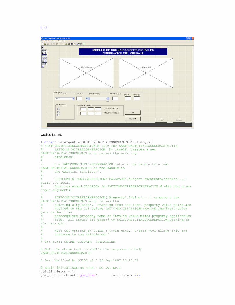
end
Codigo fuente: function varargout = SAETCOMDIGITALESGENERACION(varargin) % SAETCOMDIGITALESGENERACION M-file for SAETCOMDIGITALESGENERACION.fig % SAETCOMDIGITALESGENERACION, by itself, creates a new SAETCOMDIGITALESGENERACION or raises the existing % singleton*. % % H = SAETCOMDIGITALESGENERACION returns the handle to a new SAETCOMDIGITALESGENERACION or the handle to % the existing singleton*. % % SAETCOMDIGITALESGENERACION('CALLBACK',hObject,eventData,handles,...) calls the local % function named CALLBACK in SAETCOMDIGITALESGENERACION.M with the given input arguments. % % SAETCOMDIGITALESGENERACION('Property','Value',...) creates a new SAETCOMDIGITALESGENERACION or raises the % existing singleton*. Starting from the left, property value pairs are % applied to the GUI before SAETCOMDIGITALESGENERACION_OpeningFunction gets called. An % unrecognized property name or invalid value makes property application % stop. All inputs are passed to SAETCOMDIGITALESGENERACION_OpeningFcn via varargin. % % *See GUI Options on GUIDE's Tools menu. Choose "GUI allows only one % instance to run (singleton)". % % See also: GUIDE, GUIDATA, GUIHANDLES % Edit the above text to modify the response to help SAETCOMDIGITALESGENERACION % Last Modified by GUIDE v2.5 29-Sep-2007 16:40:37 % Begin initialization code - DO NOT EDIT gui_Singleton = 1; gui_State = struct('gui_Name', mfilename, ...

'gui_Singleton', gui_Singleton, ... 'gui_OpeningFcn', @SAETCOMDIGITALESGENERACION_OpeningFcn, ... 'gui_OutputFcn', @SAETCOMDIGITALESGENERACION_OutputFcn, ... 'gui_LayoutFcn', [] , ... 'gui_Callback', []); if nargin && ischar(varargin{1}) gui_State.gui_Callback = str2func(varargin{1}); end if nargout [varargout{1:nargout}] = gui_mainfcn(gui_State, varargin{:}); else gui_mainfcn(gui_State, varargin{:}); end % End initialization code - DO NOT EDIT % --- Executes just before SAETCOMDIGITALESGENERACION is made visible. function SAETCOMDIGITALESGENERACION_OpeningFcn(hObject, eventdata, handles, varargin) % This function has no output args, see OutputFcn. % hObject handle to figure % eventdata reserved - to be defined in a future version of MATLAB % handles structure with handles and user data (see GUIDATA) % varargin command line arguments to SAETCOMDIGITALESGENERACION (see VARARGIN) % Choose default command line output for SAETCOMDIGITALESGENERACION handles.output = hObject; % Update handles structure guidata(hObject, handles); % UIWAIT makes SAETCOMDIGITALESGENERACION wait for user response (see UIRESUME) % uiwait(handles.figure1); % --- Outputs from this function are returned to the command line. function varargout = SAETCOMDIGITALESGENERACION_OutputFcn(hObject, eventdata, handles) % varargout cell array for returning output args (see VARARGOUT); % hObject handle to figure % eventdata reserved - to be defined in a future version of MATLAB % handles structure with handles and user data (see GUIDATA) % Get default command line output from handles structure varargout{1} = handles.output; % --- Executes on selection change in ANALOGICOESCOGER. function ANALOGICOESCOGER_Callback(hObject, eventdata, handles) % hObject handle to ANALOGICOESCOGER (see GCBO) % eventdata reserved - to be defined in a future version of MATLAB % handles structure with handles and user data (see GUIDATA) % Hints: contents = get(hObject,'String') returns ANALOGICOESCOGER contents as cell array % contents{get(hObject,'Value')} returns selected item from ANALOGICOESCOGER % --- Executes during object creation, after setting all properties. function ANALOGICOESCOGER_CreateFcn(hObject, eventdata, handles) % hObject handle to ANALOGICOESCOGER (see GCBO) % eventdata reserved - to be defined in a future version of MATLAB

% handles empty - handles not created until after all CreateFcns called % Hint: popupmenu controls usually have a white background on Windows. % See ISPC and COMPUTER. if ispc && isequal(get(hObject,'BackgroundColor'), get(0,'defaultUicontrolBackgroundColor')) set(hObject,'BackgroundColor','white'); end % --- Executes on button press in ANALOGICOPROCESAR. function ANALOGICOPROCESAR_Callback(hObject, eventdata, handles) % hObject handle to ANALOGICOPROCESAR (see GCBO) % eventdata reserved - to be defined in a future version of MATLAB % handles structure with handles and user data (see GUIDATA) p=get(handles.ANALOGICOPROCESAR,'value'); if p==1, b=get(handles.ANALOGICOESCOGER,'value'); switch b case 1 %onda seno set(handles.PARAMETROSTONOS,'visible','on') set(handles.NUMTONOS,'visible','on') global Fc; global amplitud; global t; M = moviein(50); t=1/8000:1/8000:2; for j=1:50, Fc=get(handles.ANALOGICOFRECUENCIA,'value'); Fc=Fc*1000; amplitud=str2double(get(handles.ANALOGICOAMPLITUD,'String')); %validacion if isnan(amplitud) beep set(handles.ANALOGICOAMPLITUD,'String',0); amplitud=0; errordlg('El valor debe ser numérico','ERROR') end x=amplitud*sin(2*(pi/4)*Fc*(t+j)); set(handles.SENALTIEMPO,'visible','on') axes(handles.SENALTIEMPO) plot(t,x); grid AXIS([0 0.02 min(x) max(x)]) title('DOMINIO DEL TIEMPO') XLABEL('TIEMPO') YLABEL('AMPLITUD') M(:,j) = getframe; end cla global amplitud; global t; set(handles.ANALOGICOFRECUENCIA1,'string',Fc) offset=str2double(get(handles.ANALOGICOOFFSET,'String')); %validacion if isnan(offset) beep set(handles.ANALOGICOOFFSET,'String',0); offset=0; errordlg('El valor debe ser numérico','ERROR') end

fase=str2double(get(handles.ANALOGICOFASE,'String')); %validacion if isnan(fase) beep set(handles.ANALOGICOFASE,'String',0); fase=0; errordlg('El valor debe ser numérico','ERROR') end %creo la forma de onda mensaje=amplitud*sin((2*pi*Fc*t)+fase); mensaje=mensaje+offset; save datos2.mat mensaje set(handles.SENALTIEMPO,'visible','on') axes(handles.SENALTIEMPO) plot(mensaje) grid AXIS([0 200 min(mensaje) max(mensaje)]) title('DOMINIO DEL TIEMPO') XLABEL('TIEMPO') YLABEL('AMPLITUD') %ESPECTRO EN FRECUENCIA y=abs(fftshift(fft(mensaje))); y=y./length(t); w=linspace(-4000,4000,length(mensaje)); set(handles.SENALFREC,'visible','on') axes(handles.SENALFREC) plot(w,y) grid title('ESPECTRO DE FRECUENCIA') XLABEL('FRECUENCIA') YLABEL('AMPLITUD') case 2 %onda coseno set(handles.PARAMETROSTONOS,'visible','on') set(handles.NUMTONOS,'visible','on') global Fc; global amplitud; global t; M = moviein(50); t=1/8000:1/8000:2; for j=1:50, Fc=get(handles.ANALOGICOFRECUENCIA,'value'); Fc=Fc*1000; amplitud=str2double(get(handles.ANALOGICOAMPLITUD,'String')); %validacion if isnan(amplitud) beep set(handles.ANALOGICOAMPLITUD,'String',0); amplitud=0; errordlg('El valor debe ser numérico','ERROR') end x=amplitud*cos(2*(pi/4)*Fc*(t+j)); set(handles.SENALTIEMPO,'visible','on') axes(handles.SENALTIEMPO) plot(t,x,'r'); grid AXIS([0 0.02 min(x) max(x)]) title('DOMINIO DEL TIEMPO') XLABEL('TIEMPO') YLABEL('AMPLITUD') M(:,j) = getframe; end cla global amplitud; global t;

set(handles.ANALOGICOFRECUENCIA1,'string',Fc) offset=str2double(get(handles.ANALOGICOOFFSET,'String')); %validacion if isnan(offset) beep set(handles.ANALOGICOOFFSET,'String',0); offset=0; errordlg('El valor debe ser numérico','ERROR') end fase=str2double(get(handles.ANALOGICOFASE,'String')); %validacion if isnan(fase) beep set(handles.ANALOGICOFASE,'String',0); fase=0; errordlg('El valor debe ser numérico','ERROR') end %creo la forma de onda mensaje=amplitud*cos((2*pi*Fc*t)+fase); mensaje=mensaje+offset; save datos2.mat mensaje set(handles.SENALTIEMPO,'visible','on') axes(handles.SENALTIEMPO) plot(mensaje,'r') grid AXIS([0 200 min(mensaje) max(mensaje)]) title('DOMINIO DEL TIEMPO') XLABEL('TIEMPO') YLABEL('AMPLITUD') %ESPECTRO EN FRECUENCIA y=abs(fftshift(fft(mensaje))); y=y./length(t); w=linspace(-4000,4000,length(mensaje)); set(handles.SENALFREC,'visible','on') axes(handles.SENALFREC) plot(w,y) grid title('ESPECTRO DE FRECUENCIA') XLABEL('FRECUENCIA') YLABEL('AMPLITUD') case 3 %multitono seno set(handles.PARAMETROSTONOS,'visible','on') set(handles.NUMTONOS,'visible','on') global Fc; global amplitud; global t; Fc=get(handles.ANALOGICOFRECUENCIA,'value'); Fc=Fc*1000; amplitud=str2double(get(handles.ANALOGICOAMPLITUD,'String')); %validacion if isnan(amplitud) beep set(handles.ANALOGICOAMPLITUD,'String',0); amplitud=0; errordlg('El valor debe ser numérico','ERROR') end offset=str2double(get(handles.ANALOGICOOFFSET,'String'));

%validacion if isnan(offset) beep set(handles.ANALOGICOOFFSET,'String',0); offset=0; errordlg('El valor debe ser numérico','ERROR') end fase=str2double(get(handles.ANALOGICOFASE,'String')); %validacion if isnan(fase) beep set(handles.ANALOGICOFASE,'String',0); fase=0; errordlg('El valor debe ser numérico','ERROR') end set(handles.ANALOGICOFRECUENCIA1,'string',Fc) numtonos=get(handles.NUMERODETONOS,'value'); numtonos2=get(handles.NUMERODETONOS2,'value'); numtonos3=get(handles.NUMERODETONOS3,'value'); if numtonos==1, set(handles.A3,'visible','off') set(handles.F3,'visible','off') set(handles.A4,'visible','off') set(handles.F4,'visible','off') M = moviein(50); t=1/8000:1/8000:2; for j=1:50, A2=str2double(get(handles.A2,'String')); if isnan(A2) beep set(handles.A2,'String',0); A2=0; errordlg('El valor debe ser numérico','ERROR') end F2=str2double(get(handles.F2,'String')); if isnan(F2) beep set(handles.F2,'String',0); F2=0; errordlg('El valor debe ser numérico','ERROR') end x1=amplitud*(0.75)*sin(2*(pi/4)*Fc*(t+j))+A2*(0.5)*sin(2*(pi/4)*F2*(t+j)); set(handles.SENALTIEMPO,'visible','on') axes(handles.SENALTIEMPO) plot(t,x1); grid AXIS([0 0.02 min(x1) max(x1)]) title('DOMINIO DEL TIEMPO') XLABEL('TIEMPO') YLABEL('AMPLITUD') M(:,j) = getframe; end %creo la forma de onda mensaje1=amplitud*sin((2*pi*Fc*t)+fase)+A2*sin((2*pi*F2*t)+fase); mensaje1=mensaje1+offset; mensaje=mensaje1; save datos2.mat mensaje set(handles.SENALTIEMPO,'visible','on') axes(handles.SENALTIEMPO) plot(mensaje1) grid AXIS([0 200 min(mensaje1) max(mensaje1)]) title('DOMINIO DEL TIEMPO')
XLABEL('TIEMPO') YLABEL('AMPLITUD') %ESPECTRO EN FRECUENCIA y=abs(fftshift(fft(mensaje1))); y=y./length(mensaje1); w=linspace(-4000,4000,length(mensaje1)); set(handles.SENALFREC,'visible','on') axes(handles.SENALFREC) plot(w,y) grid title('ESPECTRO DE FRECUENCIA') XLABEL('FRECUENCIA') YLABEL('AMPLITUD') end if numtonos2==1, set(handles.A4,'visible','off') set(handles.F4,'visible','off') set(handles.A3,'visible','on') set(handles.F3,'visible','on') M = moviein(50); t=1/8000:1/8000:2; for j=1:50, A2=str2double(get(handles.A2,'String')); if isnan(A2) beep set(handles.A2,'String',0); A2=0; errordlg('El valor debe ser numérico','ERROR') end F2=str2double(get(handles.F2,'String')); if isnan(F2) beep set(handles.F2,'String',0); F2=0; errordlg('El valor debe ser numérico','ERROR') end A3=str2double(get(handles.A3,'String')); if isnan(A3) beep set(handles.A3,'String',0); A3=0; errordlg('El valor debe ser numérico','ERROR') end F3=str2double(get(handles.F3,'String')); if isnan(F3) beep set(handles.F3,'String',0); F3=0; errordlg('El valor debe ser numérico','ERROR') end x2=amplitud*(0.75)*sin(2*(pi/4)*Fc*(t+j))+A2*(0.5)*sin(2*(pi/4)*F2*(t+j))+A3*(0.5)*sin(2*(pi/4)*F3*(t+j)); set(handles.SENALTIEMPO,'visible','on') axes(handles.SENALTIEMPO) plot(t,x2); grid AXIS([0 0.02 min(x2) max(x2)]) title('DOMINIO DEL TIEMPO') XLABEL('TIEMPO') YLABEL('AMPLITUD') M(:,j) = getframe; end %creo la forma de onda mensaje2=amplitud*sin((2*pi*Fc*t)+fase)+A2*sin((2*pi*F2*t)+fase)+A3*sin((2*pi*F3*t)+fase); mensaje2=mensaje2+offset;

mensaje=mensaje2; save datos2.mat mensaje set(handles.SENALTIEMPO,'visible','on') axes(handles.SENALTIEMPO) plot(mensaje2) grid AXIS([0 200 min(mensaje2) max(mensaje2)]) title('DOMINIO DEL TIEMPO') XLABEL('TIEMPO') YLABEL('AMPLITUD') %ESPECTRO EN FRECUENCIA y=abs(fftshift(fft(mensaje2))); y=y./length(mensaje2); w=linspace(-4000,4000,length(mensaje2)); set(handles.SENALFREC,'visible','on') axes(handles.SENALFREC) plot(w,y) grid title('ESPECTRO DE FRECUENCIA') XLABEL('FRECUENCIA') YLABEL('AMPLITUD') end if numtonos3==1, set(handles.A4,'visible','on') set(handles.F4,'visible','on') set(handles.A3,'visible','on') set(handles.F3,'visible','on') M = moviein(50); t=1/8000:1/8000:2; for j=1:50, A2=str2double(get(handles.A2,'String')); if isnan(A2) beep set(handles.A2,'String',0); A2=0; errordlg('El valor debe ser numérico','ERROR') end F2=str2double(get(handles.F2,'String')); if isnan(F2) beep set(handles.F2,'String',0); F2=0; errordlg('El valor debe ser numérico','ERROR') end A3=str2double(get(handles.A3,'String')); if isnan(A3) beep set(handles.A3,'String',0); A3=0; errordlg('El valor debe ser numérico','ERROR') end F3=str2double(get(handles.F3,'String')); if isnan(F3) beep set(handles.F3,'String',0); F3=0; errordlg('El valor debe ser numérico','ERROR') end A4=str2double(get(handles.A4,'String')); if isnan(A4) beep set(handles.A4,'String',0); A4=0; errordlg('El valor debe ser numérico','ERROR') end F4=str2double(get(handles.F4,'String')); if isnan(F4) beep

set(handles.F4,'String',0); F4=0; errordlg('El valor debe ser numérico','ERROR') end x3=amplitud*(0.75)*sin(2*(pi/4)*Fc*(t+j))+A2*(0.5)*sin(2*(pi/4)*F2*(t+j))+A3*(0.5)*sin(2*(pi/4)*F3*(t+j))+A4*(0.5)*sin(2*(pi/4)*F4*(t+j)); set(handles.SENALTIEMPO,'visible','on') axes(handles.SENALTIEMPO) plot(t,x3); grid AXIS([0 0.02 min(x3) max(x3)]) title('DOMINIO DEL TIEMPO') XLABEL('TIEMPO') YLABEL('AMPLITUD') M(:,j) = getframe; end %creo la forma de onda mensaje3=amplitud*sin((2*pi*Fc*t)+fase)+A2*sin((2*pi*F2*t)+fase)+A3*sin((2*pi*F3*t)+fase)+A4*sin((2*pi*F4*t)+fase); mensaje3=mensaje3+offset; mensaje=mensaje3; save datos2.mat mensaje set(handles.SENALTIEMPO,'visible','on') axes(handles.SENALTIEMPO) plot(mensaje3) grid AXIS([0 200 min(mensaje3) max(mensaje3)]) title('DOMINIO DEL TIEMPO') XLABEL('TIEMPO') YLABEL('AMPLITUD') %ESPECTRO EN FRECUENCIA y=abs(fftshift(fft(mensaje3))); y=y./length(mensaje3); w=linspace(-4000,4000,length(mensaje3)); set(handles.SENALFREC,'visible','on') axes(handles.SENALFREC) plot(w,y) grid title('ESPECTRO DE FRECUENCIA') XLABEL('FRECUENCIA') YLABEL('AMPLITUD') end case 4 %multitono coseno set(handles.PARAMETROSTONOS,'visible','on') set(handles.NUMTONOS,'visible','on') global Fc; global amplitud; global t; Fc=get(handles.ANALOGICOFRECUENCIA,'value'); Fc=Fc*1000; amplitud=str2double(get(handles.ANALOGICOAMPLITUD,'String')); %validacion if isnan(amplitud) beep set(handles.ANALOGICOAMPLITUD,'String',0); amplitud=0; errordlg('El valor debe ser numérico','ERROR') end offset=str2double(get(handles.ANALOGICOOFFSET,'String')); %validacion if isnan(offset) beep set(handles.ANALOGICOOFFSET,'String',0);

offset=0; errordlg('El valor debe ser numérico','ERROR') end fase=str2double(get(handles.ANALOGICOFASE,'String')); %validacion if isnan(fase) beep set(handles.ANALOGICOFASE,'String',0); fase=0; errordlg('El valor debe ser numérico','ERROR') end set(handles.ANALOGICOFRECUENCIA1,'string',Fc) numtonos=get(handles.NUMERODETONOS,'value'); numtonos2=get(handles.NUMERODETONOS2,'value'); numtonos3=get(handles.NUMERODETONOS3,'value'); load datos2.mat if numtonos==1, set(handles.A3,'visible','off') set(handles.F3,'visible','off') set(handles.A4,'visible','off') set(handles.F4,'visible','off') M = moviein(50); t=1/8000:1/8000:2; for j=1:50, A2=str2double(get(handles.A2,'String')); if isnan(A2) beep set(handles.A2,'String',0); A2=0; errordlg('El valor debe ser numérico','ERROR') end F2=str2double(get(handles.F2,'String')); if isnan(F2) beep set(handles.F2,'String',0); F2=0; errordlg('El valor debe ser numérico','ERROR') end x1=amplitud*(0.75)*cos(2*(pi/4)*Fc*(t+j))+A2*(0.5)*cos(2*(pi/4)*F2*(t+j)); set(handles.SENALTIEMPO,'visible','on') axes(handles.SENALTIEMPO) plot(t,x1); grid AXIS([0 0.02 min(x1) max(x1)]) title('DOMINIO DEL TIEMPO') XLABEL('TIEMPO') YLABEL('AMPLITUD') M(:,j) = getframe; end %creo la forma de onda mensaje1=amplitud*cos((2*pi*Fc*t)+fase)+A2*cos((2*pi*F2*t)+fase); mensaje1=mensaje1+offset; mensaje=mensaje1; save datos2.mat mensaje set(handles.SENALTIEMPO,'visible','on') axes(handles.SENALTIEMPO) plot(mensaje1) grid AXIS([0 200 min(mensaje1) max(mensaje1)]) title('DOMINIO DEL TIEMPO') XLABEL('TIEMPO') YLABEL('AMPLITUD') %ESPECTRO EN FRECUENCIA

y=abs(fftshift(fft(mensaje1))); y=y./length(mensaje1); w=linspace(-4000,4000,length(mensaje1)); set(handles.SENALFREC,'visible','on') axes(handles.SENALFREC) plot(w,y) grid title('ESPECTRO DE FRECUENCIA') XLABEL('FRECUENCIA') YLABEL('AMPLITUD') end if numtonos2==1, set(handles.A4,'visible','off') set(handles.F4,'visible','off') set(handles.A3,'visible','on') set(handles.F3,'visible','on') M = moviein(50); t=1/8000:1/8000:2; for j=1:50, A2=str2double(get(handles.A2,'String')); if isnan(A2) beep set(handles.A2,'String',0); A2=0; errordlg('El valor debe ser numérico','ERROR') end F2=str2double(get(handles.F2,'String')); if isnan(F2) beep set(handles.F2,'String',0); F2=0; errordlg('El valor debe ser numérico','ERROR') end A3=str2double(get(handles.A3,'String')); if isnan(A3) beep set(handles.A3,'String',0); A3=0; errordlg('El valor debe ser numérico','ERROR') end F3=str2double(get(handles.F3,'String')); if isnan(F3) beep set(handles.F3,'String',0); F3=0; errordlg('El valor debe ser numérico','ERROR') end x2=amplitud*(0.75)*cos(2*(pi/4)*Fc*(t+j))+A2*(0.5)*cos(2*(pi/4)*F2*(t+j))+A3*(0.5)*cos(2*(pi/4)*F3*(t+j)); set(handles.SENALTIEMPO,'visible','on') axes(handles.SENALTIEMPO) plot(t,x2); grid AXIS([0 0.02 min(x2) max(x2)]) title('DOMINIO DEL TIEMPO') XLABEL('TIEMPO') YLABEL('AMPLITUD') M(:,j) = getframe; end %creo la forma de onda mensaje2=amplitud*cos((2*pi*Fc*t)+fase)+A2*cos((2*pi*F2*t)+fase)+A3*cos((2*pi*F3*t)+fase); mensaje2=mensaje2+offset; mensaje=mensaje2;
save datos2.mat mensaje set(handles.SENALTIEMPO,'visible','on') axes(handles.SENALTIEMPO) plot(mensaje2) grid AXIS([0 200 min(mensaje2) max(mensaje2)]) title('DOMINIO DEL TIEMPO') XLABEL('TIEMPO') YLABEL('AMPLITUD') %ESPECTRO EN FRECUENCIA y=abs(fftshift(fft(mensaje2))); y=y./length(mensaje2); w=linspace(-4000,4000,length(mensaje2)); set(handles.SENALFREC,'visible','on') axes(handles.SENALFREC) plot(w,y) grid title('ESPECTRO DE FRECUENCIA') XLABEL('FRECUENCIA') YLABEL('AMPLITUD') end if numtonos3==1, set(handles.A4,'visible','on') set(handles.F4,'visible','on') set(handles.A3,'visible','on') set(handles.F3,'visible','on') M = moviein(50); t=1/8000:1/8000:2; for j=1:50, A2=str2double(get(handles.A2,'String')); if isnan(A2) beep set(handles.A2,'String',0); A2=0; errordlg('El valor debe ser numérico','ERROR') end F2=str2double(get(handles.F2,'String')); if isnan(F2) beep set(handles.F2,'String',0); F2=0; errordlg('El valor debe ser numérico','ERROR') end A3=str2double(get(handles.A3,'String')); if isnan(A3) beep set(handles.A3,'String',0); A3=0; errordlg('El valor debe ser numérico','ERROR') end F3=str2double(get(handles.F3,'String')); if isnan(F3) beep set(handles.F3,'String',0); F3=0; errordlg('El valor debe ser numérico','ERROR') end A4=str2double(get(handles.A4,'String')); if isnan(A4) beep set(handles.A4,'String',0); A4=0; errordlg('El valor debe ser numérico','ERROR') end F4=str2double(get(handles.F4,'String')); if isnan(F4) beep set(handles.F4,'String',0);

F4=0; errordlg('El valor debe ser numérico','ERROR') end x3=amplitud*(0.75)*cos(2*(pi/4)*Fc*(t+j))+A2*(0.5)*cos(2*(pi/4)*F2*(t+j))+A3*(0.5)*cos(2*(pi/4)*F3*(t+j))+A4*(0.5)*cos(2*(pi/4)*F4*(t+j)); set(handles.SENALTIEMPO,'visible','on') axes(handles.SENALTIEMPO) plot(t,x3); grid AXIS([0 0.02 min(x3) max(x3)]) title('DOMINIO DEL TIEMPO') XLABEL('TIEMPO') YLABEL('AMPLITUD') M(:,j) = getframe; end %creo la forma de onda mensaje3=amplitud*cos((2*pi*Fc*t)+fase)+A2*cos((2*pi*F2*t)+fase)+A3*cos((2*pi*F3*t)+fase)+A4*cos((2*pi*F4*t)+fase); mensaje3=mensaje3+offset; mensaje=mensaje3; save datos2.mat mensaje set(handles.SENALTIEMPO,'visible','on') axes(handles.SENALTIEMPO) plot(mensaje3) grid AXIS([0 200 min(mensaje3) max(mensaje3)]) title('DOMINIO DEL TIEMPO') XLABEL('TIEMPO') YLABEL('AMPLITUD') %ESPECTRO EN FRECUENCIA y=abs(fftshift(fft(mensaje3))); y=y./length(mensaje3); w=linspace(-4000,4000,length(mensaje3)); set(handles.SENALFREC,'visible','on') axes(handles.SENALFREC) plot(w,y) grid title('ESPECTRO DE FRECUENCIA') XLABEL('FRECUENCIA') YLABEL('AMPLITUD') end case 5 %voz % set(handles.A2,'visible','off') % set(handles.F2,'visible','off') % set(handles.A3,'visible','off') % set(handles.F3,'visible','off') % set(handles.A4,'visible','off') % set(handles.F4,'visible','off') set(handles.PARAMETROSTONOS,'visible','off') set(handles.NUMTONOS,'visible','off') % set(handles.FASE11,'visible','off') % set(handles.CICLODETRABAJO11,'visible','off') % set(handles.CICLODETRABAJO1,'visible','off') % %G=get(handles.GRABAR1,'value'); Fs = 11025*2; voz = wavrecord(16000, Fs); %cinco seg de grabacion mensaje=voz; global t; %formadeonda1=formadeonda1(1:16000); mensaje=mensaje'; save datos2.mat mensaje wavplay(voz, Fs); set(handles.SENALTIEMPO,'visible','on')
axes(handles.SENALTIEMPO) plot(voz) grid title('DOMINIO TIEMPO') XLABEL('TIEMPO') YLABEL('AMPLITUD') %ESPECTRO EN FRECUENCIA y=abs(fftshift(fft(voz))); y=y./length(voz); w=linspace(-Fs/2,Fs/2,length(voz)); set(handles.SENALFREC,'visible','on') axes(handles.SENALFREC) plot(w,y) grid title('ESPECTRO DE FRECUENCIA') XLABEL('FRECUENCIA') YLABEL('AMPLITUD') otherwise, end end function ANALOGICOAMPLITUD_Callback(hObject, eventdata, handles) % hObject handle to ANALOGICOAMPLITUD (see GCBO) % eventdata reserved - to be defined in a future version of MATLAB % handles structure with handles and user data (see GUIDATA) % Hints: get(hObject,'String') returns contents of ANALOGICOAMPLITUD as text % str2double(get(hObject,'String')) returns contents of ANALOGICOAMPLITUD as a double % --- Executes during object creation, after setting all properties. function ANALOGICOAMPLITUD_CreateFcn(hObject, eventdata, handles) % hObject handle to ANALOGICOAMPLITUD (see GCBO) % eventdata reserved - to be defined in a future version of MATLAB % handles empty - handles not created until after all CreateFcns called % Hint: edit controls usually have a white background on Windows. % See ISPC and COMPUTER. if ispc && isequal(get(hObject,'BackgroundColor'), get(0,'defaultUicontrolBackgroundColor')) set(hObject,'BackgroundColor','white'); end % --- Executes on slider movement. function ANALOGICOFRECUENCIA_Callback(hObject, eventdata, handles) % hObject handle to ANALOGICOFRECUENCIA (see GCBO) % eventdata reserved - to be defined in a future version of MATLAB % handles structure with handles and user data (see GUIDATA) % Hints: get(hObject,'Value') returns position of slider % get(hObject,'Min') and get(hObject,'Max') to determine range of slider % --- Executes during object creation, after setting all properties. function ANALOGICOFRECUENCIA_CreateFcn(hObject, eventdata, handles) % hObject handle to ANALOGICOFRECUENCIA (see GCBO) % eventdata reserved - to be defined in a future version of MATLAB % handles empty - handles not created until after all CreateFcns called

% Hint: slider controls usually have a light gray background. if isequal(get(hObject,'BackgroundColor'), get(0,'defaultUicontrolBackgroundColor')) set(hObject,'BackgroundColor',[.9 .9 .9]); end function ANALOGICOFRECUENCIA1_Callback(hObject, eventdata, handles) % hObject handle to ANALOGICOFRECUENCIA1 (see GCBO) % eventdata reserved - to be defined in a future version of MATLAB % handles structure with handles and user data (see GUIDATA) % Hints: get(hObject,'String') returns contents of ANALOGICOFRECUENCIA1 as text % str2double(get(hObject,'String')) returns contents of ANALOGICOFRECUENCIA1 as a double % --- Executes during object creation, after setting all properties. function ANALOGICOFRECUENCIA1_CreateFcn(hObject, eventdata, handles) % hObject handle to ANALOGICOFRECUENCIA1 (see GCBO) % eventdata reserved - to be defined in a future version of MATLAB % handles empty - handles not created until after all CreateFcns called % Hint: edit controls usually have a white background on Windows. % See ISPC and COMPUTER. if ispc && isequal(get(hObject,'BackgroundColor'), get(0,'defaultUicontrolBackgroundColor')) set(hObject,'BackgroundColor','white'); end % --- Executes on button press in NUMERODETONOS. function NUMERODETONOS_Callback(hObject, eventdata, handles) % hObject handle to NUMERODETONOS (see GCBO) % eventdata reserved - to be defined in a future version of MATLAB % handles structure with handles and user data (see GUIDATA) % Hint: get(hObject,'Value') returns toggle state of NUMERODETONOS % --- Executes on button press in NUMERODETONOS2. function NUMERODETONOS2_Callback(hObject, eventdata, handles) % hObject handle to NUMERODETONOS2 (see GCBO) % eventdata reserved - to be defined in a future version of MATLAB % handles structure with handles and user data (see GUIDATA) % Hint: get(hObject,'Value') returns toggle state of NUMERODETONOS2 % --- Executes on button press in NUMERODETONOS3. function NUMERODETONOS3_Callback(hObject, eventdata, handles) % hObject handle to NUMERODETONOS3 (see GCBO) % eventdata reserved - to be defined in a future version of MATLAB % handles structure with handles and user data (see GUIDATA) % Hint: get(hObject,'Value') returns toggle state of NUMERODETONOS3 function A2_Callback(hObject, eventdata, handles) % hObject handle to A2 (see GCBO) % eventdata reserved - to be defined in a future version of MATLAB % handles structure with handles and user data (see GUIDATA) % Hints: get(hObject,'String') returns contents of A2 as text

% str2double(get(hObject,'String')) returns contents of A2 as a double % --- Executes during object creation, after setting all properties. function A2_CreateFcn(hObject, eventdata, handles) % hObject handle to A2 (see GCBO) % eventdata reserved - to be defined in a future version of MATLAB % handles empty - handles not created until after all CreateFcns called % Hint: edit controls usually have a white background on Windows. % See ISPC and COMPUTER. if ispc && isequal(get(hObject,'BackgroundColor'), get(0,'defaultUicontrolBackgroundColor')) set(hObject,'BackgroundColor','white'); end function A3_Callback(hObject, eventdata, handles) % hObject handle to A3 (see GCBO) % eventdata reserved - to be defined in a future version of MATLAB % handles structure with handles and user data (see GUIDATA) % Hints: get(hObject,'String') returns contents of A3 as text % str2double(get(hObject,'String')) returns contents of A3 as a double % --- Executes during object creation, after setting all properties. function A3_CreateFcn(hObject, eventdata, handles) % hObject handle to A3 (see GCBO) % eventdata reserved - to be defined in a future version of MATLAB % handles empty - handles not created until after all CreateFcns called % Hint: edit controls usually have a white background on Windows. % See ISPC and COMPUTER. if ispc && isequal(get(hObject,'BackgroundColor'), get(0,'defaultUicontrolBackgroundColor')) set(hObject,'BackgroundColor','white'); end function A4_Callback(hObject, eventdata, handles) % hObject handle to A4 (see GCBO) % eventdata reserved - to be defined in a future version of MATLAB % handles structure with handles and user data (see GUIDATA) % Hints: get(hObject,'String') returns contents of A4 as text % str2double(get(hObject,'String')) returns contents of A4 as a double % --- Executes during object creation, after setting all properties. function A4_CreateFcn(hObject, eventdata, handles) % hObject handle to A4 (see GCBO) % eventdata reserved - to be defined in a future version of MATLAB % handles empty - handles not created until after all CreateFcns called % Hint: edit controls usually have a white background on Windows. % See ISPC and COMPUTER. if ispc && isequal(get(hObject,'BackgroundColor'), get(0,'defaultUicontrolBackgroundColor')) set(hObject,'BackgroundColor','white'); end function F2_Callback(hObject, eventdata, handles) % hObject handle to F2 (see GCBO)

% eventdata reserved - to be defined in a future version of MATLAB % handles structure with handles and user data (see GUIDATA) % Hints: get(hObject,'String') returns contents of F2 as text % str2double(get(hObject,'String')) returns contents of F2 as a double % --- Executes during object creation, after setting all properties. function F2_CreateFcn(hObject, eventdata, handles) % hObject handle to F2 (see GCBO) % eventdata reserved - to be defined in a future version of MATLAB % handles empty - handles not created until after all CreateFcns called % Hint: edit controls usually have a white background on Windows. % See ISPC and COMPUTER. if ispc && isequal(get(hObject,'BackgroundColor'), get(0,'defaultUicontrolBackgroundColor')) set(hObject,'BackgroundColor','white'); end function F3_Callback(hObject, eventdata, handles) % hObject handle to F3 (see GCBO) % eventdata reserved - to be defined in a future version of MATLAB % handles structure with handles and user data (see GUIDATA) % Hints: get(hObject,'String') returns contents of F3 as text % str2double(get(hObject,'String')) returns contents of F3 as a double % --- Executes during object creation, after setting all properties. function F3_CreateFcn(hObject, eventdata, handles) % hObject handle to F3 (see GCBO) % eventdata reserved - to be defined in a future version of MATLAB % handles empty - handles not created until after all CreateFcns called % Hint: edit controls usually have a white background on Windows. % See ISPC and COMPUTER. if ispc && isequal(get(hObject,'BackgroundColor'), get(0,'defaultUicontrolBackgroundColor')) set(hObject,'BackgroundColor','white'); end function F4_Callback(hObject, eventdata, handles) % hObject handle to F4 (see GCBO) % eventdata reserved - to be defined in a future version of MATLAB % handles structure with handles and user data (see GUIDATA) % Hints: get(hObject,'String') returns contents of F4 as text % str2double(get(hObject,'String')) returns contents of F4 as a double % --- Executes during object creation, after setting all properties. function F4_CreateFcn(hObject, eventdata, handles) % hObject handle to F4 (see GCBO) % eventdata reserved - to be defined in a future version of MATLAB % handles empty - handles not created until after all CreateFcns called % Hint: edit controls usually have a white background on Windows. % See ISPC and COMPUTER. if ispc && isequal(get(hObject,'BackgroundColor'), get(0,'defaultUicontrolBackgroundColor')) set(hObject,'BackgroundColor','white'); end

function ANALOGICOFASE_Callback(hObject, eventdata, handles) % hObject handle to ANALOGICOFASE (see GCBO) % eventdata reserved - to be defined in a future version of MATLAB % handles structure with handles and user data (see GUIDATA) % Hints: get(hObject,'String') returns contents of ANALOGICOFASE as text % str2double(get(hObject,'String')) returns contents of ANALOGICOFASE as a double % --- Executes during object creation, after setting all properties. function ANALOGICOFASE_CreateFcn(hObject, eventdata, handles) % hObject handle to ANALOGICOFASE (see GCBO) % eventdata reserved - to be defined in a future version of MATLAB % handles empty - handles not created until after all CreateFcns called % Hint: edit controls usually have a white background on Windows. % See ISPC and COMPUTER. if ispc && isequal(get(hObject,'BackgroundColor'), get(0,'defaultUicontrolBackgroundColor')) set(hObject,'BackgroundColor','white'); end function ANALOGICOOFFSET_Callback(hObject, eventdata, handles) % hObject handle to ANALOGICOOFFSET (see GCBO) % eventdata reserved - to be defined in a future version of MATLAB % handles structure with handles and user data (see GUIDATA) % Hints: get(hObject,'String') returns contents of ANALOGICOOFFSET as text % str2double(get(hObject,'String')) returns contents of ANALOGICOOFFSET as a double % --- Executes during object creation, after setting all properties. function ANALOGICOOFFSET_CreateFcn(hObject, eventdata, handles) % hObject handle to ANALOGICOOFFSET (see GCBO) % eventdata reserved - to be defined in a future version of MATLAB % handles empty - handles not created until after all CreateFcns called % Hint: edit controls usually have a white background on Windows. % See ISPC and COMPUTER. if ispc && isequal(get(hObject,'BackgroundColor'), get(0,'defaultUicontrolBackgroundColor')) set(hObject,'BackgroundColor','white'); end % --- Executes on button press in REGRESAR. function REGRESAR_Callback(hObject, eventdata, handles) % hObject handle to REGRESAR (see GCBO) % eventdata reserved - to be defined in a future version of MATLAB % handles structure with handles and user data (see GUIDATA) REG=get(handles.REGRESAR,'value'); if REG==1, SAET end % --- Executes on button press in IRMODULACION. function IRMODULACION_Callback(hObject, eventdata, handles)

% hObject handle to IRMODULACION (see GCBO) % eventdata reserved - to be defined in a future version of MATLAB % handles structure with handles and user data (see GUIDATA) F=get(handles.IRMODULACION,'value'); if F==1, SAETCOMDIGITALESPCM end % --- Executes on button press in AYUDA. function AYUDA_Callback(hObject, eventdata, handles) % hObject handle to AYUDA (see GCBO) % eventdata reserved - to be defined in a future version of MATLAB % handles structure with handles and user data (see GUIDATA) r111=get(handles.AYUDA,'value'); if r111==1, open ('C:\Documents and Settings\javier\Mis documentos\TESIS_POSTGRADO\PARA LA TESIS\programas definitivos\ayudas\index_DIGITALGENERACION.htm') end
Codigo fuente: function varargout = SAETCOMDIGITALESPCM(varargin) % SAETCOMDIGITALESPCM M-file for SAETCOMDIGITALESPCM.fig % SAETCOMDIGITALESPCM, by itself, creates a new SAETCOMDIGITALESPCM or raises the existing % singleton*. % % H = SAETCOMDIGITALESPCM returns the handle to a new SAETCOMDIGITALESPCM or the handle to % the existing singleton*. % % SAETCOMDIGITALESPCM('CALLBACK',hObject,eventData,handles,...) calls the local

% function named CALLBACK in SAETCOMDIGITALESPCM.M with the given input arguments. % % SAETCOMDIGITALESPCM('Property','Value',...) creates a new SAETCOMDIGITALESPCM or raises the % existing singleton*. Starting from the left, property value pairs are % applied to the GUI before SAETCOMDIGITALESPCM_OpeningFunction gets called. An % unrecognized property name or invalid value makes property application % stop. All inputs are passed to SAETCOMDIGITALESPCM_OpeningFcn via varargin. % % *See GUI Options on GUIDE's Tools menu. Choose "GUI allows only one % instance to run (singleton)". % % See also: GUIDE, GUIDATA, GUIHANDLES % Edit the above text to modify the response to help SAETCOMDIGITALESPCM % Last Modified by GUIDE v2.5 29-Sep-2007 16:46:34 % Begin initialization code - DO NOT EDIT gui_Singleton = 1; gui_State = struct('gui_Name', mfilename, ... 'gui_Singleton', gui_Singleton, ... 'gui_OpeningFcn', @SAETCOMDIGITALESPCM_OpeningFcn, ... 'gui_OutputFcn', @SAETCOMDIGITALESPCM_OutputFcn, ... 'gui_LayoutFcn', [] , ... 'gui_Callback', []); if nargin && ischar(varargin{1}) gui_State.gui_Callback = str2func(varargin{1}); end if nargout [varargout{1:nargout}] = gui_mainfcn(gui_State, varargin{:}); else gui_mainfcn(gui_State, varargin{:}); end % End initialization code - DO NOT EDIT % --- Executes just before SAETCOMDIGITALESPCM is made visible. function SAETCOMDIGITALESPCM_OpeningFcn(hObject, eventdata, handles, varargin) % This function has no output args, see OutputFcn. % hObject handle to figure % eventdata reserved - to be defined in a future version of MATLAB % handles structure with handles and user data (see GUIDATA) % varargin command line arguments to SAETCOMDIGITALESPCM (see VARARGIN) set(handles.IMAGEN,'Visible','on'); axes(handles.IMAGEN); image(imread('telecom10','jpeg')); set(handles.IMAGEN,'Xtick',[]); set(handles.IMAGEN,'Ytick',[]); % Choose default command line output for SAETCOMDIGITALESPCM handles.output = hObject; % Update handles structure guidata(hObject, handles); % UIWAIT makes SAETCOMDIGITALESPCM wait for user response (see UIRESUME) % uiwait(handles.figure1); % --- Outputs from this function are returned to the command line.

function varargout = SAETCOMDIGITALESPCM_OutputFcn(hObject, eventdata, handles) % varargout cell array for returning output args (see VARARGOUT); % hObject handle to figure % eventdata reserved - to be defined in a future version of MATLAB % handles structure with handles and user data (see GUIDATA) % Get default command line output from handles structure varargout{1} = handles.output; % --- Executes on button press in REGRESAR. function REGRESAR_Callback(hObject, eventdata, handles) % hObject handle to REGRESAR (see GCBO) % eventdata reserved - to be defined in a future version of MATLAB % handles structure with handles and user data (see GUIDATA) F=get(handles.REGRESAR,'value'); if F==1, SAETCOMDIGITALESGENERACION end % --- Executes on button press in PCMPROCESAR. function PCMPROCESAR_Callback(hObject, eventdata, handles) % hObject handle to PCMPROCESAR (see GCBO) % eventdata reserved - to be defined in a future version of MATLAB % handles structure with handles and user data (see GUIDATA) principal=get(handles.PCMPROCESAR,'value'); if principal==1, %rutina para Wave_gen table_index =3 if( isempty(table_index) ) error('Experiment number must be between 1 and 8.'); elseif( (table_index <= 0) | (table_index > 8) ) error('Experiment number must be between 1 and 8.'); end table = [ 10 100 10 10 8 100 40 8 ]; SAMPLING_CONSTANT = table(table_index); BINARY_DATA_RATE = 1000; SAMPLING_FREQ = BINARY_DATA_RATE * SAMPLING_CONSTANT; CARRIER_FREQUENCY = [ 1000000 4000000 ]; NYQUIST_BLOCK = 8; % Number of blocks for Nyquist pulse generation NYQUIST_ALPHA = 0.5; % Default value of "Excessive BW factor" DUOBINARY_BLOCK = 8; % Number of blocks for Duobinary pulse. global START_OK; global SAMPLING_CONSTANT; global SAMPLING_FREQ; global BINARY_DATA_RATE; global CARRIER_FREQUENCY; global NYQUIST_BLOCK; global NYQUIST_ALPHA; global DUOBINARY_BLOCK; fprintf('===================================================================='); fprintf('\n\n'); fprintf(' In this MATLAB session default sampling frequency is set at \n\n'); fprintf('\t\t %6.2f [kHz].\n\n',SAMPLING_FREQ/1000); fprintf(' Highest frequency component that can be processed by all \n'); fprintf(' MATLAB routines is less than or equal to: \n\n');

fprintf('\t\t %6.2f [kHz].\n',SAMPLING_FREQ/2000); fprintf('\n'); fprintf('===================================================================='); fprintf('\n\n'); disp('These values will remain in effect until the "SAMPLING_FREQ" or the'); disp('"BINARY_DATA_RATE" variables are changed. If you specify Rb as the'); disp('new binary data rate, then the sampling frquency will be set to:'); fprintf('\n\t\t(%4.0f)Rb [Hz].\n',SAMPLING_CONSTANT); fprintf('\n'); % % The next two variables are for error messages only % BELL = 'fprintf(''\007\007\007'')'; WARNING = 'fprintf(''\n\t * NOT SUFFICIENT INPUT ARGUMENTS \t * USAGE:\n'')'; global BELL; global WARNING; clear table table_index; global bitsmuestra; global Fpm; Fpm=get(handles.FRECUENCIAM,'value'); Fpm=Fpm*4000; Fpm=round(Fpm); set(handles.FRECUENCIAM1,'string',Fpm) amplitudm=str2double(get(handles.AMPLITUDM,'String')); %validacion if isnan(amplitudm) beep set(handles.AMPLITUDM,'String',0); amplitudm=0; errordlg('El valor debe ser numérico','ERROR') end ciclodetrabajo=str2double(get(handles.CICLODETRABAJOM,'String')); %validacion if isnan(ciclodetrabajo) beep set(handles.CICLODETRABAJOM,'String',50); ciclodetrabajo=50; errordlg('El valor debe ser numérico','ERROR') end if (ciclodetrabajo<=0) | (ciclodetrabajo>=100) beep errordlg('El valor de ciclo de trabajo debe ser mayor que "0" y menor que "100" ','ERROR') set(handles.CICLODETRABAJOM,'String',50); ciclodetrabajo=50; end bitsmuestra=str2double(get(handles.BITSMUESTRA,'String')); %validacion if isnan(bitsmuestra) beep set(handles.BITSMUESTRA,'String',0); bitsmuestra=0; errordlg('El valor debe ser numérico','ERROR') end Q=2^bitsmuestra; set(handles.Q,'string',Q) %CREO LA SEÑAL DE MUESTREO t=1/8000:1/8000:2; smuestreo=amplitudm*square(2*pi*Fpm*t,ciclodetrabajo); smuestreo=(smuestreo+1)/2;

load datos2.mat set(handles.SENALTIEMPO,'visible','on') axes(handles.SENALTIEMPO) plot(mensaje) grid AXIS([0 200 min(mensaje) max(mensaje)]) title('DOMINIO DEL TIEMPO') XLABEL('TIEMPO') YLABEL('AMPLITUD') %ESPECTRO EN FRECUENCIA y=abs(fftshift(fft(mensaje))); y=y./length(mensaje); w=linspace(-4000,4000,length(mensaje)); set(handles.SENALFREC,'visible','on') axes(handles.SENALFREC) plot(w,y) grid title('ESPECTRO DE FRECUENCIA') XLABEL('FRECUENCIA') YLABEL('AMPLITUD') %proceso de muestreo muestra=mensaje.*smuestreo; set(handles.MUESTREOTIEMPO,'visible','on') axes(handles.MUESTREOTIEMPO) plot(muestra) hold on plot(mensaje,'r') hold off grid AXIS([0 200 min(muestra) max(muestra)]) title('DOMINIO DEL TIEMPO') XLABEL('TIEMPO') YLABEL('AMPLITUD') %ESPECTRO EN FRECUENCIA y=abs(fftshift(fft(muestra))); y=y./length(muestra); w=linspace(-4000,4000,length(muestra)); set(handles.MUESTREOFREC,'visible','on') axes(handles.MUESTREOFREC) plot(w,y) grid title('ESPECTRO DE FRECUENCIA') XLABEL('FRECUENCIA') YLABEL('AMPLITUD') %PARA LA COMPANSION C=get(handles.LEYU,'value'); if C==1, global senalC; global senalQ; global senalE; senalC=MU_LAW(muestra,255); senalQ=QUANTIZE(senalC,bitsmuestra); senalE=MU_INV(senalQ,255); set(handles.CUANTIFICACIONTIEMPO,'visible','on') axes(handles.CUANTIFICACIONTIEMPO) plot(senalE) hold on plot(mensaje,'r')

hold off grid AXIS([0 200 min(senalE) max(senalE)]) title('DOMINIO DEL TIEMPO') XLABEL('TIEMPO') YLABEL('AMPLITUD') %ESPECTRO EN FRECUENCIA y=abs(fftshift(fft(senalE))); y=y./length(senalE); w=linspace(-4000,4000,length(senalE)); set(handles.CUANTIFICACIONFREC,'visible','on') axes(handles.CUANTIFICACIONFREC) plot(w,y) grid title('ESPECTRO DE FRECUENCIA') XLABEL('FRECUENCIA') YLABEL('AMPLITUD') ERRORQ=senalQ-muestra; poterrorQ=mean(ERRORQ.*ERRORQ); set(handles.ERRORQ,'string',poterrorQ) SAETCOMDIGITALESCOMPANSION %CODIFICO LA SEÑAL % senalE=round(senalE); % senalE=abs(senalE); set(handles.CODIFICO,'string',bitsmuestra) codificacion=BIN_ENC(senalQ,bitsmuestra); msg1=reshape(codificacion',(length(codificacion)*bitsmuestra),1); save datos6.mat msg1 codigoL=get(handles.CODIGOLINEA,'value'); switch codigoL case 1 %unipolar_NRZ X = WAVE_GEN(msg1,'unipolar_nrz',Fpm*bitsmuestra); save datos5.mat X set(handles.CODIFICACIONTIEMPO,'visible','on') axes(handles.CODIFICACIONTIEMPO) plot(X) grid title('SEÑAL EN TIEMPO') XLABEL('TIEMPO') YLABEL('AMPLITUD') AXIS([0 400 -3 3]) hold on plot(mensaje,'r') hold off % c=xcorr(X,X); dep1=abs(fftshift(fft(X))).*abs(fftshift(fft(X))); dep1=dep1./length(X); w2=linspace(-5000,5000,length(dep1)); set(handles.CODIFICACIONFREC,'visible','on') axes(handles.CODIFICACIONFREC) plot(w2,dep1) grid title('ESPECTRO DE FRECUENCIA') XLABEL('FRECUENCIA') YLABEL('AMPLITUD') case 2 %unipolar RZ X = WAVE_GEN(msg1,'unipolar_rz',Fpm*bitsmuestra);
save datos5.mat X set(handles.CODIFICACIONTIEMPO,'visible','on') axes(handles.CODIFICACIONTIEMPO) plot(X) grid title('SEÑAL EN TIEMPO') XLABEL('TIEMPO') YLABEL('AMPLITUD') AXIS([0 400 -3 3]) hold on plot(mensaje,'r') hold off % c=xcorr(X,X); dep1=abs(fftshift(fft(X))).*abs(fftshift(fft(X))); dep1=dep1./length(X); w2=linspace(-5000,5000,length(dep1)); set(handles.CODIFICACIONFREC,'visible','on') axes(handles.CODIFICACIONFREC) plot(w2,dep1/length(dep1)) grid title('ESPECTRO DE FRECUENCIA') XLABEL('FRECUENCIA') YLABEL('AMPLITUD') case 3 %polar nrz X = WAVE_GEN(msg1,'polar_nrz',Fpm*bitsmuestra); save datos5.mat X set(handles.CODIFICACIONTIEMPO,'visible','on') axes(handles.CODIFICACIONTIEMPO) plot(X) grid title('SEÑAL EN TIEMPO') XLABEL('TIEMPO') YLABEL('AMPLITUD') AXIS([0 400 -3 3]) hold on plot(mensaje,'r') hold off % c=xcorr(X,X); dep1=abs(fftshift(fft(X))).*abs(fftshift(fft(X))); dep1=dep1./length(X); w2=linspace(-5000,5000,length(dep1)); set(handles.CODIFICACIONFREC,'visible','on') axes(handles.CODIFICACIONFREC) plot(w2,dep1) grid title('ESPECTRO DE FRECUENCIA') XLABEL('FRECUENCIA') YLABEL('AMPLITUD') case 4 %polar rz X = WAVE_GEN(msg1,'polar_rz',Fpm*bitsmuestra); save datos5.mat X set(handles.CODIFICACIONTIEMPO,'visible','on') axes(handles.CODIFICACIONTIEMPO) plot(X) grid title('SEÑAL EN TIEMPO') XLABEL('TIEMPO') YLABEL('AMPLITUD') AXIS([0 400 -3 3]) hold on plot(mensaje,'r')

hold off % c=xcorr(X,X); dep1=abs(fftshift(fft(X))).*abs(fftshift(fft(X))); dep1=dep1./length(X); w2=linspace(-5000,5000,length(dep1)); set(handles.CODIFICACIONFREC,'visible','on') axes(handles.CODIFICACIONFREC) plot(w2,dep1) grid title('ESPECTRO DE FRECUENCIA') XLABEL('FRECUENCIA') YLABEL('AMPLITUD') case 5 %bipolar NRZ X = WAVE_GEN(msg1,'bipolar_nrz',Fpm*bitsmuestra); save datos5.mat X set(handles.CODIFICACIONTIEMPO,'visible','on') axes(handles.CODIFICACIONTIEMPO) plot(X) grid title('SEÑAL EN TIEMPO') XLABEL('TIEMPO') YLABEL('AMPLITUD') AXIS([0 400 -5 5]) hold on plot(mensaje,'r') hold off % c=xcorr(X,X); dep1=abs(fftshift(fft(X))).*abs(fftshift(fft(X))); dep1=dep1./length(X); w2=linspace(-5000,5000,length(dep1)); set(handles.CODIFICACIONFREC,'visible','on') axes(handles.CODIFICACIONFREC) plot(w2,dep1) grid title('ESPECTRO DE FRECUENCIA') XLABEL('FRECUENCIA') YLABEL('AMPLITUD') case 6 %bipolar rz X = WAVE_GEN(msg1,'polar_rz',Fpm*bitsmuestra); save datos5.mat X set(handles.CODIFICACIONTIEMPO,'visible','on') axes(handles.CODIFICACIONTIEMPO) plot(X) grid title('SEÑAL EN TIEMPO') XLABEL('TIEMPO') YLABEL('AMPLITUD') AXIS([0 400 -3 3]) hold on plot(mensaje,'r') hold off % c=xcorr(X,X); dep1=abs(fftshift(fft(X))).*abs(fftshift(fft(X))); dep1=dep1./length(X); w2=linspace(-5000,5000,length(dep1)); set(handles.CODIFICACIONFREC,'visible','on') axes(handles.CODIFICACIONFREC) plot(w2,dep1) grid title('ESPECTRO DE FRECUENCIA') XLABEL('FRECUENCIA')
YLABEL('AMPLITUD') case 7 %manchester X = WAVE_GEN(msg1,'manchester',Fpm*bitsmuestra); save datos5.mat X set(handles.CODIFICACIONTIEMPO,'visible','on') axes(handles.CODIFICACIONTIEMPO) plot(X) grid title('SEÑAL EN TIEMPO') XLABEL('TIEMPO') YLABEL('AMPLITUD') AXIS([0 400 -3 3]) hold on plot(mensaje,'r') hold off % c=xcorr(X,X); dep1=abs(fftshift(fft(X))).*abs(fftshift(fft(X))); dep1=dep1./length(X); w2=linspace(-5000,5000,length(dep1)); set(handles.CODIFICACIONFREC,'visible','on') axes(handles.CODIFICACIONFREC) plot(w2,dep1) grid title('ESPECTRO DE FRECUENCIA') XLABEL('FRECUENCIA') YLABEL('AMPLITUD') otherwise, end SAETCOMDIGITALESCODIFICACION end if C==0, senalQ=QUANTIZE(muestra,bitsmuestra); % senalQ1 = UENCODE(muestra,bitsmuestra); set(handles.CUANTIFICACIONTIEMPO,'visible','on') axes(handles.CUANTIFICACIONTIEMPO) plot(senalQ) % hold on % plot(mensaje,'r') % hold off grid AXIS([0 200 min(senalQ) max(senalQ)]) title('DOMINIO DEL TIEMPO') XLABEL('TIEMPO') YLABEL('AMPLITUD') %ESPECTRO EN FRECUENCIA y=abs(fftshift(fft(senalQ))); y=y./length(senalQ); w=linspace(-4000,4000,length(senalQ)); set(handles.CUANTIFICACIONFREC,'visible','on') axes(handles.CUANTIFICACIONFREC) plot(w,y) grid title('ESPECTRO DE FRECUENCIA') XLABEL('FRECUENCIA')

YLABEL('AMPLITUD') ERRORQ=senalQ-muestra; poterrorQ=mean(ERRORQ.*ERRORQ); set(handles.ERRORQ,'string',poterrorQ) set(handles.CODIFICO,'string',bitsmuestra) %CODIFICO LA SEÑAL codificacion=BIN_ENC(senalQ,bitsmuestra); msg1=reshape(codificacion',(length(codificacion)*bitsmuestra),1); save datos6.mat msg1 set(handles.CODIFICACIONTIEMPO,'visible','on') axes(handles.CODIFICACIONTIEMPO) codigoL=get(handles.CODIGOLINEA,'value'); switch codigoL case 1 %unipolar_NRZ X = WAVE_GEN(msg1,'unipolar_nrz',Fpm*bitsmuestra); save datos5.mat X set(handles.CODIFICACIONTIEMPO,'visible','on') axes(handles.CODIFICACIONTIEMPO) plot(X) grid title('SEÑAL EN TIEMPO') XLABEL('TIEMPO') YLABEL('AMPLITUD') AXIS([0 400 -3 3]) hold on plot(mensaje,'r') hold off % c=xcorr(X,X); dep1=abs(fftshift(fft(X))).*abs(fftshift(fft(X))); dep1=dep1./length(X); w2=linspace(-5000,5000,length(dep1)); set(handles.CODIFICACIONFREC,'visible','on') axes(handles.CODIFICACIONFREC) plot(w2,dep1) grid title('ESPECTRO DE FRECUENCIA') XLABEL('FRECUENCIA') YLABEL('AMPLITUD') case 2 %unipolar RZ X = WAVE_GEN(msg1,'unipolar_rz',Fpm*bitsmuestra); save datos5.mat X set(handles.CODIFICACIONTIEMPO,'visible','on') axes(handles.CODIFICACIONTIEMPO) plot(X) grid title('SEÑAL EN TIEMPO') XLABEL('TIEMPO') YLABEL('AMPLITUD') AXIS([0 400 -3 3]) hold on plot(mensaje,'r') hold off % c=xcorr(X,X); dep1=abs(fftshift(fft(X))).*abs(fftshift(fft(X))); dep1=dep1./length(X); w2=linspace(-5000,5000,length(dep1)); set(handles.CODIFICACIONFREC,'visible','on') axes(handles.CODIFICACIONFREC) plot(w2,dep1) grid

title('ESPECTRO DE FRECUENCIA') XLABEL('FRECUENCIA') YLABEL('AMPLITUD') case 3 %polar nrz X = WAVE_GEN(msg1,'polar_nrz',Fpm*bitsmuestra); save datos5.mat X set(handles.CODIFICACIONTIEMPO,'visible','on') axes(handles.CODIFICACIONTIEMPO) plot(X) grid title('SEÑAL EN TIEMPO') XLABEL('TIEMPO') YLABEL('AMPLITUD') AXIS([0 400 -3 3]) hold on plot(mensaje,'r') hold off % c=xcorr(X,X); dep1=abs(fftshift(fft(X))).*abs(fftshift(fft(X))); dep1=dep1./length(X); w2=linspace(-5000,5000,length(dep1)); set(handles.CODIFICACIONFREC,'visible','on') axes(handles.CODIFICACIONFREC) plot(w2,dep1) grid title('ESPECTRO DE FRECUENCIA') XLABEL('FRECUENCIA') YLABEL('AMPLITUD') case 4 %polar rz X = WAVE_GEN(msg1,'polar_rz',Fpm*bitsmuestra); save datos5.mat X set(handles.CODIFICACIONTIEMPO,'visible','on') axes(handles.CODIFICACIONTIEMPO) plot(X) grid title('SEÑAL EN TIEMPO') XLABEL('TIEMPO') YLABEL('AMPLITUD') AXIS([0 400 -3 3]) hold on plot(mensaje,'r') hold off % c=xcorr(X,X); dep1=abs(fftshift(fft(X))).*abs(fftshift(fft(X))); dep1=dep1./length(X); w2=linspace(-5000,5000,length(dep1)); set(handles.CODIFICACIONFREC,'visible','on') axes(handles.CODIFICACIONFREC) plot(w2,dep1) grid title('ESPECTRO DE FRECUENCIA') XLABEL('FRECUENCIA') YLABEL('AMPLITUD') case 5 %bipolar NRZ X = WAVE_GEN(msg1,'bipolar_nrz',Fpm*bitsmuestra); save datos5.mat X set(handles.CODIFICACIONTIEMPO,'visible','on') axes(handles.CODIFICACIONTIEMPO) plot(X) grid

title('SEÑAL EN TIEMPO') XLABEL('TIEMPO') YLABEL('AMPLITUD') AXIS([0 400 -3 3]) hold on plot(mensaje,'r') hold off % c=xcorr(X,X); dep1=abs(fftshift(fft(X))).*abs(fftshift(fft(X))); dep1=dep1./length(X); w2=linspace(-5000,5000,length(dep1)); set(handles.CODIFICACIONFREC,'visible','on') axes(handles.CODIFICACIONFREC) plot(w2,dep1) grid title('ESPECTRO DE FRECUENCIA') XLABEL('FRECUENCIA') YLABEL('AMPLITUD') case 6 %bipolar rz X = WAVE_GEN(msg1,'polar_rz',Fpm*bitsmuestra); save datos5.mat X set(handles.CODIFICACIONTIEMPO,'visible','on') axes(handles.CODIFICACIONTIEMPO) plot(X) grid title('SEÑAL EN TIEMPO') XLABEL('TIEMPO') YLABEL('AMPLITUD') AXIS([0 400 -3 3]) hold on plot(mensaje,'r') hold off % c=xcorr(X,X); dep1=abs(fftshift(fft(X))).*abs(fftshift(fft(X))); dep1=dep1./length(X); w2=linspace(-5000,5000,length(dep1)); set(handles.CODIFICACIONFREC,'visible','on') axes(handles.CODIFICACIONFREC) plot(w2,dep1) grid title('ESPECTRO DE FRECUENCIA') XLABEL('FRECUENCIA') YLABEL('AMPLITUD') case 7 %manchester X = WAVE_GEN(msg1,'manchester',Fpm*bitsmuestra); save datos5.mat X set(handles.CODIFICACIONTIEMPO,'visible','on') axes(handles.CODIFICACIONTIEMPO) plot(X) grid title('SEÑAL EN TIEMPO') XLABEL('TIEMPO') YLABEL('AMPLITUD') AXIS([0 400 -3 3]) hold on plot(mensaje,'r') hold off % c=xcorr(X,X); dep1=abs(fftshift(fft(X))).*abs(fftshift(fft(X))); dep1=dep1./length(X); w2=linspace(-5000,5000,length(dep1));

set(handles.CODIFICACIONFREC,'visible','on') axes(handles.CODIFICACIONFREC) plot(w2,dep1) grid title('ESPECTRO DE FRECUENCIA') XLABEL('FRECUENCIA') YLABEL('AMPLITUD') otherwise, end SAETCOMDIGITALESCODIFICACION end end % --- Executes on button press in IRMODULACION. function IRMODULACION_Callback(hObject, eventdata, handles) % hObject handle to IRMODULACION (see GCBO) % eventdata reserved - to be defined in a future version of MATLAB % handles structure with handles and user data (see GUIDATA) F=get(handles.IRMODULACION,'value'); if F==1, SAETCOMDIGITALMODULACION end function AMPLITUDM_Callback(hObject, eventdata, handles) % hObject handle to AMPLITUDM (see GCBO) % eventdata reserved - to be defined in a future version of MATLAB % handles structure with handles and user data (see GUIDATA) % Hints: get(hObject,'String') returns contents of AMPLITUDM as text % str2double(get(hObject,'String')) returns contents of AMPLITUDM as a double % --- Executes during object creation, after setting all properties. function AMPLITUDM_CreateFcn(hObject, eventdata, handles) % hObject handle to AMPLITUDM (see GCBO) % eventdata reserved - to be defined in a future version of MATLAB % handles empty - handles not created until after all CreateFcns called % Hint: edit controls usually have a white background on Windows. % See ISPC and COMPUTER. if ispc && isequal(get(hObject,'BackgroundColor'), get(0,'defaultUicontrolBackgroundColor')) set(hObject,'BackgroundColor','white'); end % --- Executes on slider movement. function FRECUENCIAM_Callback(hObject, eventdata, handles) % hObject handle to FRECUENCIAM (see GCBO) % eventdata reserved - to be defined in a future version of MATLAB % handles structure with handles and user data (see GUIDATA) % Hints: get(hObject,'Value') returns position of slider % get(hObject,'Min') and get(hObject,'Max') to determine range of slider % --- Executes during object creation, after setting all properties.

function FRECUENCIAM_CreateFcn(hObject, eventdata, handles) % hObject handle to FRECUENCIAM (see GCBO) % eventdata reserved - to be defined in a future version of MATLAB % handles empty - handles not created until after all CreateFcns called % Hint: slider controls usually have a light gray background. if isequal(get(hObject,'BackgroundColor'), get(0,'defaultUicontrolBackgroundColor')) set(hObject,'BackgroundColor',[.9 .9 .9]); end function CICLODETRABAJOM_Callback(hObject, eventdata, handles) % hObject handle to CICLODETRABAJOM (see GCBO) % eventdata reserved - to be defined in a future version of MATLAB % handles structure with handles and user data (see GUIDATA) % Hints: get(hObject,'String') returns contents of CICLODETRABAJOM as text % str2double(get(hObject,'String')) returns contents of CICLODETRABAJOM as a double % --- Executes during object creation, after setting all properties. function CICLODETRABAJOM_CreateFcn(hObject, eventdata, handles) % hObject handle to CICLODETRABAJOM (see GCBO) % eventdata reserved - to be defined in a future version of MATLAB % handles empty - handles not created until after all CreateFcns called % Hint: edit controls usually have a white background on Windows. % See ISPC and COMPUTER. if ispc && isequal(get(hObject,'BackgroundColor'), get(0,'defaultUicontrolBackgroundColor')) set(hObject,'BackgroundColor','white'); end function BITSMUESTRA_Callback(hObject, eventdata, handles) % hObject handle to BITSMUESTRA (see GCBO) % eventdata reserved - to be defined in a future version of MATLAB % handles structure with handles and user data (see GUIDATA) % Hints: get(hObject,'String') returns contents of BITSMUESTRA as text % str2double(get(hObject,'String')) returns contents of BITSMUESTRA as a double % --- Executes during object creation, after setting all properties. function BITSMUESTRA_CreateFcn(hObject, eventdata, handles) % hObject handle to BITSMUESTRA (see GCBO) % eventdata reserved - to be defined in a future version of MATLAB % handles empty - handles not created until after all CreateFcns called % Hint: edit controls usually have a white background on Windows. % See ISPC and COMPUTER. if ispc && isequal(get(hObject,'BackgroundColor'), get(0,'defaultUicontrolBackgroundColor')) set(hObject,'BackgroundColor','white'); end % --- Executes on button press in LEYU. function LEYU_Callback(hObject, eventdata, handles) % hObject handle to LEYU (see GCBO) % eventdata reserved - to be defined in a future version of MATLAB % handles structure with handles and user data (see GUIDATA)

% Hint: get(hObject,'Value') returns toggle state of LEYU % --- Executes on selection change in CODIGOLINEA. function CODIGOLINEA_Callback(hObject, eventdata, handles) % hObject handle to CODIGOLINEA (see GCBO) % eventdata reserved - to be defined in a future version of MATLAB % handles structure with handles and user data (see GUIDATA) % Hints: contents = get(hObject,'String') returns CODIGOLINEA contents as cell array % contents{get(hObject,'Value')} returns selected item from CODIGOLINEA % --- Executes during object creation, after setting all properties. function CODIGOLINEA_CreateFcn(hObject, eventdata, handles) % hObject handle to CODIGOLINEA (see GCBO) % eventdata reserved - to be defined in a future version of MATLAB % handles empty - handles not created until after all CreateFcns called % Hint: popupmenu controls usually have a white background on Windows. % See ISPC and COMPUTER. if ispc && isequal(get(hObject,'BackgroundColor'), get(0,'defaultUicontrolBackgroundColor')) set(hObject,'BackgroundColor','white'); end % --- Executes on button press in AYUDA. function AYUDA_Callback(hObject, eventdata, handles) % hObject handle to AYUDA (see GCBO) % eventdata reserved - to be defined in a future version of MATLAB % handles structure with handles and user data (see GUIDATA) r111=get(handles.AYUDA,'value'); if r111==1, open ('C:\Documents and Settings\javier\Mis documentos\TESIS_POSTGRADO\PARA LA TESIS\programas definitivos\ayudas\index_DIGITALPCM.htm') end

Codigo fuente: function varargout = SAETCOMDIGITALMODULACION(varargin) % SAETCOMDIGITALMODULACION M-file for SAETCOMDIGITALMODULACION.fig % SAETCOMDIGITALMODULACION, by itself, creates a new SAETCOMDIGITALMODULACION or raises the existing % singleton*. % % H = SAETCOMDIGITALMODULACION returns the handle to a new SAETCOMDIGITALMODULACION or the handle to % the existing singleton*. % % SAETCOMDIGITALMODULACION('CALLBACK',hObject,eventData,handles,...) calls the local % function named CALLBACK in SAETCOMDIGITALMODULACION.M with the given input arguments. % % SAETCOMDIGITALMODULACION('Property','Value',...) creates a new SAETCOMDIGITALMODULACION or raises the % existing singleton*. Starting from the left, property value pairs are % applied to the GUI before SAETCOMDIGITALMODULACION_OpeningFunction gets called. An % unrecognized property name or invalid value makes property application % stop. All inputs are passed to SAETCOMDIGITALMODULACION_OpeningFcn via varargin. % % *See GUI Options on GUIDE's Tools menu. Choose "GUI allows only one % instance to run (singleton)". % % See also: GUIDE, GUIDATA, GUIHANDLES % Edit the above text to modify the response to help SAETCOMDIGITALMODULACION % Last Modified by GUIDE v2.5 29-Sep-2007 16:57:59 % Begin initialization code - DO NOT EDIT gui_Singleton = 1; gui_State = struct('gui_Name', mfilename, ... 'gui_Singleton', gui_Singleton, ... 'gui_OpeningFcn', @SAETCOMDIGITALMODULACION_OpeningFcn, ... 'gui_OutputFcn', @SAETCOMDIGITALMODULACION_OutputFcn, ... 'gui_LayoutFcn', [] , ... 'gui_Callback', []); if nargin && ischar(varargin{1}) gui_State.gui_Callback = str2func(varargin{1}); end if nargout [varargout{1:nargout}] = gui_mainfcn(gui_State, varargin{:}); else gui_mainfcn(gui_State, varargin{:}); end % End initialization code - DO NOT EDIT % --- Executes just before SAETCOMDIGITALMODULACION is made visible. function SAETCOMDIGITALMODULACION_OpeningFcn(hObject, eventdata, handles, varargin) % This function has no output args, see OutputFcn. % hObject handle to figure % eventdata reserved - to be defined in a future version of MATLAB % handles structure with handles and user data (see GUIDATA) % varargin command line arguments to SAETCOMDIGITALMODULACION (see VARARGIN) % Choose default command line output for SAETCOMDIGITALMODULACION handles.output = hObject;

% Update handles structure guidata(hObject, handles); % UIWAIT makes SAETCOMDIGITALMODULACION wait for user response (see UIRESUME) % uiwait(handles.figure1); % --- Outputs from this function are returned to the command line. function varargout = SAETCOMDIGITALMODULACION_OutputFcn(hObject, eventdata, handles) % varargout cell array for returning output args (see VARARGOUT); % hObject handle to figure % eventdata reserved - to be defined in a future version of MATLAB % handles structure with handles and user data (see GUIDATA) % Get default command line output from handles structure varargout{1} = handles.output; function AMPPORTADORA_Callback(hObject, eventdata, handles) % hObject handle to AMPPORTADORA (see GCBO) % eventdata reserved - to be defined in a future version of MATLAB % handles structure with handles and user data (see GUIDATA) % Hints: get(hObject,'String') returns contents of AMPPORTADORA as text % str2double(get(hObject,'String')) returns contents of AMPPORTADORA as a double % --- Executes during object creation, after setting all properties. function AMPPORTADORA_CreateFcn(hObject, eventdata, handles) % hObject handle to AMPPORTADORA (see GCBO) % eventdata reserved - to be defined in a future version of MATLAB % handles empty - handles not created until after all CreateFcns called % Hint: edit controls usually have a white background on Windows. % See ISPC and COMPUTER. if ispc && isequal(get(hObject,'BackgroundColor'), get(0,'defaultUicontrolBackgroundColor')) set(hObject,'BackgroundColor','white'); end % --- Executes on slider movement. function FRECUENCIAP_Callback(hObject, eventdata, handles) % hObject handle to FRECUENCIAP (see GCBO) % eventdata reserved - to be defined in a future version of MATLAB % handles structure with handles and user data (see GUIDATA) % Hints: get(hObject,'Value') returns position of slider % get(hObject,'Min') and get(hObject,'Max') to determine range of slider % --- Executes during object creation, after setting all properties. function FRECUENCIAP_CreateFcn(hObject, eventdata, handles) % hObject handle to FRECUENCIAP (see GCBO) % eventdata reserved - to be defined in a future version of MATLAB % handles empty - handles not created until after all CreateFcns called % Hint: slider controls usually have a light gray background. if isequal(get(hObject,'BackgroundColor'), get(0,'defaultUicontrolBackgroundColor')) set(hObject,'BackgroundColor',[.9 .9 .9]); end

function FASEMODULACION_Callback(hObject, eventdata, handles) % hObject handle to FASEMODULACION (see GCBO) % eventdata reserved - to be defined in a future version of MATLAB % handles structure with handles and user data (see GUIDATA) % Hints: get(hObject,'String') returns contents of FASEMODULACION as text % str2double(get(hObject,'String')) returns contents of FASEMODULACION as a double % --- Executes during object creation, after setting all properties. function FASEMODULACION_CreateFcn(hObject, eventdata, handles) % hObject handle to FASEMODULACION (see GCBO) % eventdata reserved - to be defined in a future version of MATLAB % handles empty - handles not created until after all CreateFcns called % Hint: edit controls usually have a white background on Windows. % See ISPC and COMPUTER. if ispc && isequal(get(hObject,'BackgroundColor'), get(0,'defaultUicontrolBackgroundColor')) set(hObject,'BackgroundColor','white'); end % --- Executes on selection change in TIPODEMODULACION. function TIPODEMODULACION_Callback(hObject, eventdata, handles) % hObject handle to TIPODEMODULACION (see GCBO) % eventdata reserved - to be defined in a future version of MATLAB % handles structure with handles and user data (see GUIDATA) % Hints: contents = get(hObject,'String') returns TIPODEMODULACION contents as cell array % contents{get(hObject,'Value')} returns selected item from TIPODEMODULACION % --- Executes during object creation, after setting all properties. function TIPODEMODULACION_CreateFcn(hObject, eventdata, handles) % hObject handle to TIPODEMODULACION (see GCBO) % eventdata reserved - to be defined in a future version of MATLAB % handles empty - handles not created until after all CreateFcns called % Hint: popupmenu controls usually have a white background on Windows. % See ISPC and COMPUTER. if ispc && isequal(get(hObject,'BackgroundColor'), get(0,'defaultUicontrolBackgroundColor')) set(hObject,'BackgroundColor','white'); end function DESVIACIONFREC_Callback(hObject, eventdata, handles) % hObject handle to DESVIACIONFREC (see GCBO) % eventdata reserved - to be defined in a future version of MATLAB % handles structure with handles and user data (see GUIDATA) % Hints: get(hObject,'String') returns contents of DESVIACIONFREC as text % str2double(get(hObject,'String')) returns contents of DESVIACIONFREC as a double % --- Executes during object creation, after setting all properties. function DESVIACIONFREC_CreateFcn(hObject, eventdata, handles) % hObject handle to DESVIACIONFREC (see GCBO) % eventdata reserved - to be defined in a future version of MATLAB % handles empty - handles not created until after all CreateFcns called

% Hint: edit controls usually have a white background on Windows. % See ISPC and COMPUTER. if ispc && isequal(get(hObject,'BackgroundColor'), get(0,'defaultUicontrolBackgroundColor')) set(hObject,'BackgroundColor','white'); end % --- Executes on button press in MODULACIONPROCESAR. function MODULACIONPROCESAR_Callback(hObject, eventdata, handles) % hObject handle to MODULACIONPROCESAR (see GCBO) % eventdata reserved - to be defined in a future version of MATLAB % handles structure with handles and user data (see GUIDATA) p=get(handles.MODULACIONPROCESAR,'value'); if p==1, global tipo; tipo=get(handles.TIPODEMODULACION,'value'); switch tipo case 1 %ask global FP; global AP; t=1/8000:1/8000:(16000)/8000; FP=get(handles.FRECUENCIAP,'value'); FP=FP*2000; set(handles.MOSTRARFRECUENCIA,'string',FP) AP=str2double(get(handles.AMPPORTADORA,'String')); %validacion if isnan(AP) beep set(handles.AMPPORTADORA,'String',0); AP=0; errordlg('El valor debe ser numérico','ERROR') end fase=str2double(get(handles.FASEMODULACION,'String')); %validacion if isnan(fase) beep set(handles.FASEMODULACION,'String',0); fase=0; errordlg('El valor debe ser numérico','ERROR') end load datos5.mat global mensaje; %NORMALIZO mensaje=X; % mensaje=mensaje-mean(mensaje); %sin dc set(handles.MENSAJETIEMPO,'visible','on') axes(handles.MENSAJETIEMPO) plot(mensaje) grid AXIS([0 400 -2 2]) title('DOMINIO DEL TIEMPO') XLABEL('TIEMPO') YLABEL('AMPLITUD') %ESPECTRO EN FRECUENCIA y=abs(fftshift(fft(mensaje))).*abs(fftshift(fft(mensaje))); y=y./length(mensaje); w=linspace(-4000,4000,length(mensaje)); set(handles.MENSAJEFREC,'visible','on') axes(handles.MENSAJEFREC) plot(w,y) grid title('ESPECTRO DE FRECUENCIA')

XLABEL('FRECUENCIA') YLABEL('AMPLITUD') %modulacion port1=AP*cos(2*pi*FP*t); mensaje=mensaje(1:length(port1)); xask=mensaje.*port1'; modulacion = xask'; save datos7.mat modulacion set(handles.MODULACIONTIEMPO,'visible','on') axes(handles.MODULACIONTIEMPO) plot(modulacion) hold on plot(mensaje,'r') hold off grid AXIS([0 400 (min(modulacion)-2) (max(modulacion)+2)]) title('DOMINIO DEL TIEMPO') XLABEL('TIEMPO') YLABEL('AMPLITUD') %espectro y=abs(fftshift(fft(modulacion))).*abs(fftshift(fft(modulacion))); y=y./length(modulacion); w=linspace(-4000,4000,length(modulacion)); set(handles.MODULACIONFREC,'visible','on') axes(handles.MODULACIONFREC) plot(w,y) grid title('ESPECTRO DE FRECUENCIA') XLABEL('FRECUENCIA') YLABEL('AMPLITUD') %para la constelacion ASK(OOK) global Rb; if min(mensaje)==0, modulacion1=[]; modulacion=modulacion; for i=1:length(modulacion), if modulacion(1,i)<=0, modulacion1(1,i)=0; else modulacion1(1,i)=modulacion(1,i); end end men=[(sqrt((min(modulacion1)).*(1/Rb))) (sqrt(((max(modulacion1)*max(modulacion1))/2).*(1/Rb)))]; save datos9.mat men h=SCATTERPLOT(men,1,0,'bo') grid hold on SCATTERPLOT(men,1,0,'-c',h) title('CONSTELACION IDEAL') hold off else % if (((max(mensaje)+min(mensaje))==0)&(mean(X)==0)), % men=[(-sqrt(abs(min(modulacion)).*(1/Rb))) 0 (sqrt(((max(modulacion)*max(modulacion))/2).*(1/Rb)))]; % % h=SCATTERPLOT(men,1,0,'ro') % grid % men1=[0 (sqrt(((max(modulacion)*max(modulacion))/2).*(1/Rb)))]; % hold on

% SCATTERPLOT(men1,1,0,'ro',h) % hold off % else men=[(-sqrt(abs(min(modulacion)).*(1/Rb))) (sqrt(((max(modulacion)*max(modulacion))/2).*(1/Rb)))]; save datos9.mat men h=SCATTERPLOT(men,1,0,'bo') grid hold on SCATTERPLOT(men,1,0,'-c',h) title('CONSTELACION IDEAL') hold off end case 2 %FSK ortogonal global FP; global AP; global desviacion; t=1/8000:1/8000:(16000)/8000; FP=get(handles.FRECUENCIAP,'value'); FP=FP*2000; set(handles.MOSTRARFRECUENCIA,'string',FP) AP=str2double(get(handles.AMPPORTADORA,'String')); %validacion if isnan(AP) beep set(handles.AMPPORTADORA,'String',0); AP=0; errordlg('El valor debe ser numérico','ERROR') end fase=str2double(get(handles.FASEMODULACION,'String')); %validacion if isnan(fase) beep set(handles.FASEMODULACION,'String',0); fase=0; errordlg('El valor debe ser numérico','ERROR') end desviacion=str2double(get(handles.DESVIACIONFREC,'String')); %validacion if isnan(desviacion) beep set(handles.DESVIACIONFREC,'String',1); desviacion=1; errordlg('El valor debe ser numérico','ERROR') end load datos5.mat %NORMALIZO mensaje=X; % mensaje=mensaje-mean(mensaje); %sin dc set(handles.MENSAJETIEMPO,'visible','on') axes(handles.MENSAJETIEMPO) plot(mensaje) grid AXIS([0 400 -2 2]) title('DOMINIO DEL TIEMPO') XLABEL('TIEMPO') YLABEL('AMPLITUD') %ESPECTRO EN FRECUENCIA y=abs(fftshift(fft(mensaje))).*abs(fftshift(fft(mensaje))); y=y./length(mensaje); w=linspace(-4000,4000,length(mensaje)); set(handles.MENSAJEFREC,'visible','on')
axes(handles.MENSAJEFREC) plot(w,y) grid title('ESPECTRO DE FRECUENCIA') XLABEL('FRECUENCIA') YLABEL('AMPLITUD') %modulacion port1=AP*cos(2*pi*FP*t); port2=AP*cos(2*pi*desviacion*FP*t); mensaje=mensaje(1:length(port1)); mensajeneg=not(mensaje); xask1=mensaje.*port1'; xask2=mensajeneg.*port2'; modulacion = xask1'+xask2'; save datos7.mat modulacion set(handles.MODULACIONTIEMPO,'visible','on') axes(handles.MODULACIONTIEMPO) plot(modulacion) hold on plot(mensaje,'r') hold off grid AXIS([0 400 (min(modulacion)-2) (max(modulacion)+2)]) title('DOMINIO DEL TIEMPO') XLABEL('TIEMPO') YLABEL('AMPLITUD') %espectro y=abs(fftshift(fft(modulacion))).*abs(fftshift(fft(modulacion))); y=y./length(modulacion); w=linspace(-4000,4000,length(modulacion)); set(handles.MODULACIONFREC,'visible','on') axes(handles.MODULACIONFREC) plot(w,y) grid title('ESPECTRO DE FRECUENCIA') XLABEL('FRECUENCIA') YLABEL('AMPLITUD') %para la constelacion fsk(ortogonal) global Rb; if min(mensaje)==0, % men=[(sqrt(((max(port1)*max(port1))/2).*(1/Rb))) (sqrt(((max(port2)*max(port2))/2).*(1/Rb)))*j]; save datos9.mat men h=SCATTERPLOT(men,1,0,'bo') grid hold on SCATTERPLOT(men,1,0,'-c',h) title('CONSTELACION IDEAL') hold off % else % % if (((max(mensaje)+min(mensaje))==0)&(mean(X)==0)), % % men=[(-sqrt(abs(min(modulacion)).*(1/Rb))) 0 (sqrt(((max(modulacion)*max(modulacion))/2).*(1/Rb)))]; % % % % h=SCATTERPLOT(men,1,0,'ro') % % grid % % men1=[0 (sqrt(((max(modulacion)*max(modulacion))/2).*(1/Rb)))]; % % hold on

% % SCATTERPLOT(men1,1,0,'ro',h) % % hold off % % else % men=[(-sqrt(abs(min(modulacion)).*(1/Rb))) (sqrt(((max(modulacion)*max(modulacion))/2).*(1/Rb)))]; % SCATTERPLOT(men,1,0,'go') % grid end case 3 %PSK global FP; global AP; t=1/8000:1/8000:(16000)/8000; FP=get(handles.FRECUENCIAP,'value'); FP=FP*2000; set(handles.MOSTRARFRECUENCIA,'string',FP) AP=str2double(get(handles.AMPPORTADORA,'String')); %validacion if isnan(AP) beep set(handles.AMPPORTADORA,'String',0); AP=0; errordlg('El valor debe ser numérico','ERROR') end fase=str2double(get(handles.FASEMODULACION,'String')); %validacion if isnan(fase) beep set(handles.FASEMODULACION,'String',0); fase=0; errordlg('El valor debe ser numérico','ERROR') end load datos5.mat %NORMALIZO mensaje=X; % mensaje=mensaje-mean(mensaje); %sin dc set(handles.MENSAJETIEMPO,'visible','on') axes(handles.MENSAJETIEMPO) plot(mensaje) grid AXIS([0 400 -2 2]) title('DOMINIO DEL TIEMPO') XLABEL('TIEMPO') YLABEL('AMPLITUD') %ESPECTRO EN FRECUENCIA y=abs(fftshift(fft(mensaje))).*abs(fftshift(fft(mensaje))); y=y./length(mensaje); w=linspace(-4000,4000,length(mensaje)); set(handles.MENSAJEFREC,'visible','on') axes(handles.MENSAJEFREC) plot(w,y) grid title('ESPECTRO DE FRECUENCIA') XLABEL('FRECUENCIA') YLABEL('AMPLITUD') %modulacion port1=AP*cos(2*pi*FP*t); port2=-AP*cos(2*pi*FP*t); mensaje=mensaje(1:length(port1)); mensajeneg=not(mensaje); xask1=mensaje.*port1';

xask2=mensajeneg.*port2'; modulacion = xask1'+xask2'; save datos7.mat modulacion set(handles.MODULACIONTIEMPO,'visible','on') axes(handles.MODULACIONTIEMPO) plot(modulacion) hold on plot(mensaje,'r') hold off grid AXIS([0 400 (min(modulacion)-2) (max(modulacion)+2)]) title('DOMINIO DEL TIEMPO') XLABEL('TIEMPO') YLABEL('AMPLITUD') %espectro y=abs(fftshift(fft(modulacion))).*abs(fftshift(fft(modulacion))); y=y./length(modulacion); w=linspace(-4000,4000,length(modulacion)); set(handles.MODULACIONFREC,'visible','on') axes(handles.MODULACIONFREC) plot(w,y) grid title('ESPECTRO DE FRECUENCIA') XLABEL('FRECUENCIA') YLABEL('AMPLITUD') %para la constelacion fsk(ortogonal) global Rb; % men=[(-sqrt(((max(port1)*max(port1))/2).*(1/Rb))) (sqrt(((max(port2)*max(port2))/2).*(1/Rb)))]; save datos9.mat men h=SCATTERPLOT(men,1,0,'bo') grid hold on SCATTERPLOT(men,1,0,'-c',h) title('CONSTELACION IDEAL') hold off % else % % if (((max(mensaje)+min(mensaje))==0)&(mean(X)==0)), % % men=[(-sqrt(abs(min(modulacion)).*(1/Rb))) 0 (sqrt(((max(modulacion)*max(modulacion))/2).*(1/Rb)))]; % % % % h=SCATTERPLOT(men,1,0,'ro') % % grid % % men1=[0 (sqrt(((max(modulacion)*max(modulacion))/2).*(1/Rb)))]; % % hold on % % SCATTERPLOT(men1,1,0,'ro',h) % % hold off % % else % men=[(-sqrt(abs(min(modulacion)).*(1/Rb))) (sqrt(((max(modulacion)*max(modulacion))/2).*(1/Rb)))]; % SCATTERPLOT(men,1,0,'go') % grid

otherwise, end end % --- Executes on button press in MODULACIONREGRESAR. function MODULACIONREGRESAR_Callback(hObject, eventdata, handles) % hObject handle to MODULACIONREGRESAR (see GCBO) % eventdata reserved - to be defined in a future version of MATLAB % handles structure with handles and user data (see GUIDATA) R=get(handles.MODULACIONREGRESAR,'value'); if R==1, SAETCOMDIGITALESPCM end function FS_Callback(hObject, eventdata, handles) % hObject handle to FS (see GCBO) % eventdata reserved - to be defined in a future version of MATLAB % handles structure with handles and user data (see GUIDATA) % Hints: get(hObject,'String') returns contents of FS as text % str2double(get(hObject,'String')) returns contents of FS as a double % --- Executes during object creation, after setting all properties. function FS_CreateFcn(hObject, eventdata, handles) % hObject handle to FS (see GCBO) % eventdata reserved - to be defined in a future version of MATLAB % handles empty - handles not created until after all CreateFcns called % Hint: edit controls usually have a white background on Windows. % See ISPC and COMPUTER. if ispc && isequal(get(hObject,'BackgroundColor'), get(0,'defaultUicontrolBackgroundColor')) set(hObject,'BackgroundColor','white'); end % --- Executes on button press in IRCANAL. function IRCANAL_Callback(hObject, eventdata, handles) % hObject handle to IRCANAL (see GCBO) % eventdata reserved - to be defined in a future version of MATLAB % handles structure with handles and user data (see GUIDATA) C=get(handles.IRCANAL,'value'); if C==1, SAETCOMDIGITALCANAL end % --- Executes on button press in AYUDA. function AYUDA_Callback(hObject, eventdata, handles) % hObject handle to AYUDA (see GCBO) % eventdata reserved - to be defined in a future version of MATLAB % handles structure with handles and user data (see GUIDATA) r111=get(handles.AYUDA,'value'); if r111==1, open ('C:\Documents and Settings\javier\Mis documentos\TESIS_POSTGRADO\PARA LA TESIS\programas definitivos\ayudas\index_DIGITALMODULACION.htm')

end
Codigo fuente: function varargout = SAETCOMDIGITALCANAL(varargin) % SAETCOMDIGITALCANAL M-file for SAETCOMDIGITALCANAL.fig % SAETCOMDIGITALCANAL, by itself, creates a new SAETCOMDIGITALCANAL or raises the existing % singleton*. % % H = SAETCOMDIGITALCANAL returns the handle to a new SAETCOMDIGITALCANAL or the handle to % the existing singleton*. % % SAETCOMDIGITALCANAL('CALLBACK',hObject,eventData,handles,...) calls the local % function named CALLBACK in SAETCOMDIGITALCANAL.M with the given input arguments. % % SAETCOMDIGITALCANAL('Property','Value',...) creates a new SAETCOMDIGITALCANAL or raises the % existing singleton*. Starting from the left, property value pairs are % applied to the GUI before SAETCOMDIGITALCANAL_OpeningFunction gets called. An % unrecognized property name or invalid value makes property application % stop. All inputs are passed to SAETCOMDIGITALCANAL_OpeningFcn via varargin. % % *See GUI Options on GUIDE's Tools menu. Choose "GUI allows only one % instance to run (singleton)". % % See also: GUIDE, GUIDATA, GUIHANDLES % Edit the above text to modify the response to help SAETCOMDIGITALCANAL % Last Modified by GUIDE v2.5 29-Sep-2007 17:05:25 % Begin initialization code - DO NOT EDIT gui_Singleton = 1;

gui_State = struct('gui_Name', mfilename, ... 'gui_Singleton', gui_Singleton, ... 'gui_OpeningFcn', @SAETCOMDIGITALCANAL_OpeningFcn, ... 'gui_OutputFcn', @SAETCOMDIGITALCANAL_OutputFcn, ... 'gui_LayoutFcn', [] , ... 'gui_Callback', []); if nargin && ischar(varargin{1}) gui_State.gui_Callback = str2func(varargin{1}); end if nargout [varargout{1:nargout}] = gui_mainfcn(gui_State, varargin{:}); else gui_mainfcn(gui_State, varargin{:}); end % End initialization code - DO NOT EDIT % --- Executes just before SAETCOMDIGITALCANAL is made visible. function SAETCOMDIGITALCANAL_OpeningFcn(hObject, eventdata, handles, varargin) % This function has no output args, see OutputFcn. % hObject handle to figure % eventdata reserved - to be defined in a future version of MATLAB % handles structure with handles and user data (see GUIDATA) % varargin command line arguments to SAETCOMDIGITALCANAL (see VARARGIN) % Choose default command line output for SAETCOMDIGITALCANAL handles.output = hObject; % Update handles structure guidata(hObject, handles); % UIWAIT makes SAETCOMDIGITALCANAL wait for user response (see UIRESUME) % uiwait(handles.figure1); % --- Outputs from this function are returned to the command line. function varargout = SAETCOMDIGITALCANAL_OutputFcn(hObject, eventdata, handles) % varargout cell array for returning output args (see VARARGOUT); % hObject handle to figure % eventdata reserved - to be defined in a future version of MATLAB % handles structure with handles and user data (see GUIDATA) % Get default command line output from handles structure varargout{1} = handles.output; % --- Executes on slider movement. function ABA_Callback(hObject, eventdata, handles) % hObject handle to ABA (see GCBO) % eventdata reserved - to be defined in a future version of MATLAB % handles structure with handles and user data (see GUIDATA) % Hints: get(hObject,'Value') returns position of slider % get(hObject,'Min') and get(hObject,'Max') to determine range of slider % --- Executes during object creation, after setting all properties. function ABA_CreateFcn(hObject, eventdata, handles) % hObject handle to ABA (see GCBO) % eventdata reserved - to be defined in a future version of MATLAB % handles empty - handles not created until after all CreateFcns called % Hint: slider controls usually have a light gray background. if isequal(get(hObject,'BackgroundColor'), get(0,'defaultUicontrolBackgroundColor'))

set(hObject,'BackgroundColor',[.9 .9 .9]); end % --- Executes on slider movement. function ATENUACION_Callback(hObject, eventdata, handles) % hObject handle to ATENUACION (see GCBO) % eventdata reserved - to be defined in a future version of MATLAB % handles structure with handles and user data (see GUIDATA) % Hints: get(hObject,'Value') returns position of slider % get(hObject,'Min') and get(hObject,'Max') to determine range of slider % --- Executes during object creation, after setting all properties. function ATENUACION_CreateFcn(hObject, eventdata, handles) % hObject handle to ATENUACION (see GCBO) % eventdata reserved - to be defined in a future version of MATLAB % handles empty - handles not created until after all CreateFcns called % Hint: slider controls usually have a light gray background. if isequal(get(hObject,'BackgroundColor'), get(0,'defaultUicontrolBackgroundColor')) set(hObject,'BackgroundColor',[.9 .9 .9]); end % --- Executes on slider movement. function NIVELRUIDO_Callback(hObject, eventdata, handles) % hObject handle to NIVELRUIDO (see GCBO) % eventdata reserved - to be defined in a future version of MATLAB % handles structure with handles and user data (see GUIDATA) % Hints: get(hObject,'Value') returns position of slider % get(hObject,'Min') and get(hObject,'Max') to determine range of slider % --- Executes during object creation, after setting all properties. function NIVELRUIDO_CreateFcn(hObject, eventdata, handles) % hObject handle to NIVELRUIDO (see GCBO) % eventdata reserved - to be defined in a future version of MATLAB % handles empty - handles not created until after all CreateFcns called % Hint: slider controls usually have a light gray background. if isequal(get(hObject,'BackgroundColor'), get(0,'defaultUicontrolBackgroundColor')) set(hObject,'BackgroundColor',[.9 .9 .9]); end % --- Executes on button press in ACTIVACIONCANAL. function ACTIVACIONCANAL_Callback(hObject, eventdata, handles) % hObject handle to ACTIVACIONCANAL (see GCBO) % eventdata reserved - to be defined in a future version of MATLAB % handles structure with handles and user data (see GUIDATA) % Hint: get(hObject,'Value') returns toggle state of ACTIVACIONCANAL activacion=get(handles.ACTIVACIONCANAL,'value'); switch activacion case 0 %desactivado queda normal load datos7.mat set(handles.CANALTIEMPO,'visible','on')
axes(handles.CANALTIEMPO) plot(modulacion) grid AXIS([0 200 min(modulacion) max(modulacion)]) title('DOMINIO DEL TIEMPO SIN EFECTO DEL CANAL') XLABEL('TIEMPO') YLABEL('AMPLITUD') save datos8.mat modulacion %esoectro y=abs(fftshift(fft(modulacion))); y=y./length(modulacion); w=linspace(-4000,4000,length(modulacion)); set(handles.CANALFREC,'visible','on') axes(handles.CANALFREC) plot(w,y) grid title('ESPECTRO DE FRECUENCIA SIN EFECTO DEL CANAL') XLABEL('FRECUENCIA') YLABEL('AMPLITUD') %CALCULO DE LAS PORTENCIAS DC stx=mean(modulacion.*modulacion); stxdbm=10*log10(stx/0.001); srx=mean(modulacion.*modulacion); srxdbm=10*log10(srx/0.001); nr=mean(0.*0); senalaruidor=(srx/nr)-1; senalaruidordb=10*log10(senalaruidor); set(handles.ST,'string',stx) set(handles.STDB,'string',stxdbm) set(handles.SR,'string',srx) set(handles.SRDBM,'string',srxdbm) set(handles.SNR,'string',senalaruidor) set(handles.SNRDB,'string',senalaruidordb) case 1 %afectado por el canal Fcorte=get(handles.ABA,'value'); Fcorte=Fcorte*4000; atenuacion=get(handles.ATENUACION,'value'); atenuacion=atenuacion*20; % atenuacion=round(atenuacion); nivelruido=get(handles.NIVELRUIDO,'value'); nivelruido=nivelruido*(5); set(handles.ABA1,'string',Fcorte) set(handles.ATENUACION1,'string',atenuacion) set(handles.NIVELRUIDO1,'string',nivelruido) load datos7.mat stx=mean(modulacion.*modulacion); stxdbm=10*log10(stx/0.001); %filtro de canal [B,A] = BUTTER(3,Fcorte/4000); senalf1=filter(B,A,modulacion); modulacion=senalf1; modulacion=modulacion./atenuacion; global ruido; ruido=nivelruido.*randn(1,length(modulacion)); % save datos10.mat ruido % modulacion=awgn(modulacion,nivelruido,3,'linear'); modulacion=modulacion+ruido; save datos8.mat modulacion set(handles.CANALTIEMPO,'visible','on') axes(handles.CANALTIEMPO)

plot(modulacion) grid AXIS([0 200 min(modulacion) max(modulacion)]) title('DOMINIO DEL TIEMPO') XLABEL('TIEMPO') YLABEL('AMPLITUD') %esoectro y=abs(fftshift(fft(modulacion))); y=y./length(modulacion); w=linspace(-4000,4000,length(modulacion)); set(handles.CANALFREC,'visible','on') axes(handles.CANALFREC) plot(w,y) grid title('ESPECTRO DE FRECUENCIA') XLABEL('FRECUENCIA') YLABEL('AMPLITUD') srx=mean(modulacion.*modulacion); srxdbm=10*log10(srx/0.001); nr=mean(ruido.*ruido); senalaruidor=(srx/nr)-1; senalaruidordb=10*log10(senalaruidor); set(handles.ST,'string',stx) set(handles.STDB,'string',stxdbm) set(handles.SR,'string',srx) set(handles.SRDBM,'string',srxdbm) set(handles.SNR,'string',senalaruidor) set(handles.SNRDB,'string',senalaruidordb) load datos9.mat global tipo; switch tipo case 1 %ASK %para la constelacion ASK(OOK) global Rb; global mensaje; if min(mensaje)==0, modulacion1=[]; modulacion=modulacion; for i=1:length(modulacion), if modulacion(1,i)<=0, modulacion1(1,i)=0; else modulacion1(1,i)=modulacion(1,i); end end menruido=[(sqrt(abs((min(modulacion1+ruido)).*(1/Rb)))) (sqrt(((max(modulacion1)*max(modulacion1))/2).*(1/Rb)))]; global h; h=SCATTERPLOT(men,1,0,'bo') grid hold on scatterplot(menruido,1,0,'r+',h); % Plot +'s scatterplot(menruido,1,0,'mx',h); % Plot x's scatterplot(menruido,1,0,'b.',h); % Plot dots SCATTERPLOT(menruido,1,0,'-c',h) title('CONSTELACION') hold off h = legend('sin ruido','con efecto de ruido',2); else menruido=[(-sqrt(abs((min(modulacion+ruido)).*(1/Rb)))) (sqrt(((max(modulacion)*max(modulacion))/2).*(1/Rb)))];
global h; h=SCATTERPLOT(men,1,0,'bo') grid hold on scatterplot(menruido,1,0,'r+',h); % Plot +'s scatterplot(menruido,1,0,'mx',h); % Plot x's scatterplot(menruido,1,0,'b.',h); % Plot dots SCATTERPLOT(menruido,1,0,'-c',h) title('CONSTELACION') hold off h = legend('sin ruido','con efecto de ruido',2); end case 2 %FSK ortogonal global Rb; global mensaje; if min(mensaje)==0, % menruido=[(sqrt(((max(modulacion)*max(modulacion))/2).*(1/Rb))) (sqrt(((max(modulacion)*max(modulacion))/2).*(1/Rb)))*j]; global h; h=SCATTERPLOT(men,1,0,'bo') grid hold on scatterplot(menruido,1,0,'r+',h); % Plot +'s scatterplot(menruido,1,0,'mx',h); % Plot x's scatterplot(menruido,1,0,'b.',h); % Plot dots SCATTERPLOT(menruido,1,0,'-c',h) title('CONSTELACION') hold off h = legend('sin ruido','con efecto de ruido',2); end case 3 %PSK global Rb; menruido=[(-sqrt(((max(modulacion)*max(modulacion))/2).*(1/Rb))) (sqrt(((max(modulacion)*max(modulacion))/2).*(1/Rb)))]; global h; h=SCATTERPLOT(men,1,0,'bo') grid hold on scatterplot(menruido,1,0,'r+',h); % Plot +'s scatterplot(menruido,1,0,'mx',h); % Plot x's scatterplot(menruido,1,0,'b.',h); % Plot dots SCATTERPLOT(menruido,1,0,'-c',h) title('CONSTELACION') hold off b = legend('sin ruido','con efecto de ruido',2); otherwise, end otherwise, end % --- Executes on button press in REGRESAR. function REGRESAR_Callback(hObject, eventdata, handles) % hObject handle to REGRESAR (see GCBO) % eventdata reserved - to be defined in a future version of MATLAB

% handles structure with handles and user data (see GUIDATA) P=get(handles.REGRESAR,'value'); if P==1, SAETCOMDIGITALMODULACION end % --- Executes on button press in BORRAR. function BORRAR_Callback(hObject, eventdata, handles) % hObject handle to BORRAR (see GCBO) % eventdata reserved - to be defined in a future version of MATLAB % handles structure with handles and user data (see GUIDATA) b=get(handles.BORRAR,'value'); if b==1, clf end % --- Executes on button press in IRDETECCION. function IRDETECCION_Callback(hObject, eventdata, handles) % hObject handle to IRDETECCION (see GCBO) % eventdata reserved - to be defined in a future version of MATLAB % handles structure with handles and user data (see GUIDATA) f=get(handles.IRDETECCION,'value'); if f==1, SAETCOMDIGITALDETECCION end % --- Executes on button press in AYUDA. function AYUDA_Callback(hObject, eventdata, handles) % hObject handle to AYUDA (see GCBO) % eventdata reserved - to be defined in a future version of MATLAB % handles structure with handles and user data (see GUIDATA) r111=get(handles.AYUDA,'value'); if r111==1, open ('C:\Documents and Settings\javier\Mis documentos\TESIS_POSTGRADO\PARA LA TESIS\programas definitivos\ayudas\index_DIGITALCANAL.htm') end

Codigo fuente: function varargout = SAETCOMDIGITALDETECCION(varargin) % SAETCOMDIGITALDETECCION M-file for SAETCOMDIGITALDETECCION.fig % SAETCOMDIGITALDETECCION, by itself, creates a new SAETCOMDIGITALDETECCION or raises the existing % singleton*. % % H = SAETCOMDIGITALDETECCION returns the handle to a new SAETCOMDIGITALDETECCION or the handle to % the existing singleton*. % % SAETCOMDIGITALDETECCION('CALLBACK',hObject,eventData,handles,...) calls the local % function named CALLBACK in SAETCOMDIGITALDETECCION.M with the given input arguments. % % SAETCOMDIGITALDETECCION('Property','Value',...) creates a new SAETCOMDIGITALDETECCION or raises the % existing singleton*. Starting from the left, property value pairs are % applied to the GUI before SAETCOMDIGITALDETECCION_OpeningFunction gets called. An % unrecognized property name or invalid value makes property application % stop. All inputs are passed to SAETCOMDIGITALDETECCION_OpeningFcn via varargin. % % *See GUI Options on GUIDE's Tools menu. Choose "GUI allows only one % instance to run (singleton)". % % See also: GUIDE, GUIDATA, GUIHANDLES % Edit the above text to modify the response to help SAETCOMDIGITALDETECCION % Last Modified by GUIDE v2.5 29-Sep-2007 17:17:00 % Begin initialization code - DO NOT EDIT gui_Singleton = 1; gui_State = struct('gui_Name', mfilename, ... 'gui_Singleton', gui_Singleton, ... 'gui_OpeningFcn', @SAETCOMDIGITALDETECCION_OpeningFcn, ... 'gui_OutputFcn', @SAETCOMDIGITALDETECCION_OutputFcn, ... 'gui_LayoutFcn', [] , ...
'gui_Callback', []); if nargin && ischar(varargin{1}) gui_State.gui_Callback = str2func(varargin{1}); end if nargout [varargout{1:nargout}] = gui_mainfcn(gui_State, varargin{:}); else gui_mainfcn(gui_State, varargin{:}); end % End initialization code - DO NOT EDIT % --- Executes just before SAETCOMDIGITALDETECCION is made visible. function SAETCOMDIGITALDETECCION_OpeningFcn(hObject, eventdata, handles, varargin) % This function has no output args, see OutputFcn. % hObject handle to figure % eventdata reserved - to be defined in a future version of MATLAB % handles structure with handles and user data (see GUIDATA) % varargin command line arguments to SAETCOMDIGITALDETECCION (see VARARGIN) % Choose default command line output for SAETCOMDIGITALDETECCION handles.output = hObject; % Update handles structure guidata(hObject, handles); % UIWAIT makes SAETCOMDIGITALDETECCION wait for user response (see UIRESUME) % uiwait(handles.figure1); % --- Outputs from this function are returned to the command line. function varargout = SAETCOMDIGITALDETECCION_OutputFcn(hObject, eventdata, handles) % varargout cell array for returning output args (see VARARGOUT); % hObject handle to figure % eventdata reserved - to be defined in a future version of MATLAB % handles structure with handles and user data (see GUIDATA) % Get default command line output from handles structure varargout{1} = handles.output; % --- Executes on selection change in TIPODEMODULACION. function TIPODEMODULACION_Callback(hObject, eventdata, handles) % hObject handle to TIPODEMODULACION (see GCBO) % eventdata reserved - to be defined in a future version of MATLAB % handles structure with handles and user data (see GUIDATA) % Hints: contents = get(hObject,'String') returns TIPODEMODULACION contents as cell array % contents{get(hObject,'Value')} returns selected item from TIPODEMODULACION global tipo; tipo=get(handles.TIPODEMODULACION,'value'); switch tipo case 1 %ask set(handles.TIPODETECCION,'visible','on') set(handles.TIPODETECCION1,'visible','on') global tipodeteccion; tipodeteccion=get(handles.TIPODETECCION,'value'); switch tipodeteccion case 1 %deteccion COHERENTE set(handles.CONTROL2,'visible','off') load datos8.mat

set(handles.SRTIEMPO,'visible','on') axes(handles.SRTIEMPO) plot(modulacion) grid AXIS([0 400 min(modulacion) max(modulacion)]) title('DOMINIO DEL TIEMPO') XLABEL('TIEMPO') YLABEL('AMPLITUD') %espectro y=abs(fftshift(fft(modulacion))).*abs(fftshift(fft(modulacion))); y=y./length(modulacion); w=linspace(-4000,4000,length(modulacion)); set(handles.SRFREC,'visible','on') axes(handles.SRFREC) plot(w,y) grid title('ESPECTRO DE FRECUENCIA ') XLABEL('FRECUENCIA') YLABEL('AMPLITUD') %se pasa por el sistema pasabanda global N; global Wn1; global Wn2; N=str2double(get(handles.ORDEN,'String')); %validacion if isnan(N) beep set(handles.ORDEN,'String',1); N=1; errordlg('El valor debe ser numérico','ERROR') end if (N<=0)|(N>20) beep set(handles.ORDEN,'String',1); N=1; errordlg('El valor del orden del filtro debe ser mayor que "0" y menor que "21" ','ERROR') end Wn1=str2double(get(handles.FC1,'String')); if isnan(Wn1) beep set(handles.FC1,'String',0); Wn1=0; errordlg('El valor debe ser numérico','ERROR') end if (Wn1<0)|(Wn1>3999) beep set(handles.FC1,'String',0); Wn1=0; errordlg('El valor del orden del filtro debe ser mayor que "0" y menor que "3999Hz" ','ERROR') end Wn1=Wn1/4000; Wn2=str2double(get(handles.FC2,'String')); if isnan(Wn2) beep set(handles.FC2,'String',0); Wn2=0; errordlg('El valor debe ser numérico','ERROR') end if (Wn2<0)|(Wn2>3999) beep
set(handles.FC2,'String',0); Wn2=0; errordlg('El valor de la frecuencia de corte del filtro debe ser mayor que "0" y menor que "3999Hz" ','ERROR') end Wn2=Wn2/4000; Wn=[Wn1 Wn2]; [B,A] = BUTTER(N,[Wn1 Wn2]); senalf1=filter(B,A,modulacion); modulacion=senalf1; set(handles.SRPASABANDATIEMPO,'visible','on') axes(handles.SRPASABANDATIEMPO) plot(modulacion) grid AXIS([0 400 min(modulacion) max(modulacion)]) title('DOMINIO DEL TIEMPO') XLABEL('TIEMPO') YLABEL('AMPLITUD') %espectro y=abs(fftshift(fft(modulacion))).*abs(fftshift(fft(modulacion))); y=y./length(modulacion); w=linspace(-4000,4000,length(modulacion)); set(handles.SRPASABANDAFREC,'visible','on') axes(handles.SRPASABANDAFREC) plot(w,y) grid title('ESPECTRO DE FRECUENCIA ') XLABEL('FRECUENCIA') YLABEL('AMPLITUD') %DETECCION SINCRONA global AP; global FP; global t; OL=AP*cos(2*pi*FP*t); % OL=OL'; % det=modulacion.*OL; modulacion=det; set(handles.DETECCIONTIEMPO,'visible','on') axes(handles.DETECCIONTIEMPO) plot(modulacion) grid AXIS([0 400 min(modulacion) max(modulacion)]) title('DOMINIO DEL TIEMPO') XLABEL('TIEMPO') YLABEL('AMPLITUD') %espectro y=abs(fftshift(fft(modulacion))).*abs(fftshift(fft(modulacion))); y=y./length(modulacion); w=linspace(-4000,4000,length(modulacion)); set(handles.DETECCIONFREC,'visible','on') axes(handles.DETECCIONFREC) plot(w,y) grid title('ESPECTRO DE FRECUENCIA ') XLABEL('FRECUENCIA') YLABEL('AMPLITUD') %FILTRAJE FINAL PARA RECUPERACION DEL %MENSAJE global N; global Wn; set(handles.RECUPERACION,'visible','on')

N=str2double(get(handles.ORDENF,'String')); %validacion if isnan(N) beep set(handles.ORDENF,'String',1); N=1; errordlg('El valor debe ser numérico','ERROR') end if (N<=0)|(N>20) beep set(handles.ORDENF,'String',1); N=1; errordlg('El valor del orden del filtro debe ser mayor que "0" y menor que "21" ','ERROR') end Wn=str2double(get(handles.FC,'String')); if isnan(Wn) beep set(handles.FC,'String',0); Wn=0; errordlg('El valor debe ser numérico','ERROR') end if (Wn<0)|(Wn>3999) beep set(handles.FC,'String',1); Wn=1; errordlg('El valor de la frecuencia de corte del filtro debe ser mayor que "0" y menor que "3999Hz" ','ERROR') end Wn=Wn/4000; [B,A] = BUTTER(N,Wn); senalf1=filter(B,A,modulacion); modulacion=senalf1; modulacion=modulacion'; modulacion=modulacion-mean(modulacion); set(handles.DETECCIONTIEMPO,'visible','on') axes(handles.DETECCIONTIEMPO) plot(modulacion) grid AXIS([0 400 min(modulacion) max(modulacion)]) title('DOMINIO DEL TIEMPO') XLABEL('TIEMPO') YLABEL('AMPLITUD') %espectro y=abs(fftshift(fft(modulacion))).*abs(fftshift(fft(modulacion))); y=y./length(modulacion); w=linspace(-4000,4000,length(modulacion)); set(handles.DETECCIONFREC,'visible','on') axes(handles.DETECCIONFREC) plot(w,y) grid title('ESPECTRO DE FRECUENCIA ') XLABEL('FRECUENCIA') YLABEL('AMPLITUD') load datos5.mat mensaje=X; mensaje=mensaje(1:length(modulacion)); %COMPARACION FINAL CON UMBRAL DE TD recup=[]; for j=1:length(senalf1), if modulacion(j,1)>((max(modulacion)-min(modulacion))/5)

recup(j,1)=1; else if min(mensaje)==0, recup(j,1)=0; else recup(j,1)=-1; end end end set(handles.DESTINOTIEMPO,'visible','on') axes(handles.DESTINOTIEMPO) plot(recup) hold on mensaje=mensaje(1:length(recup)); plot(mensaje+1,'r') hold off grid AXIS([0 400 -3 3]) title('DOMINIO DEL TIEMPO') XLABEL('TIEMPO') YLABEL('AMPLITUD') h = legend('RECUPERADA','ORIGINAL',2); %ESPECTRO y=abs(fftshift(fft(modulacion))); y=y./length(modulacion); w=linspace(-4000,4000,length(modulacion)); set(handles.DESTINOFREC,'visible','on') axes(handles.DESTINOFREC) plot(w,y) grid title('ESPECTRO DE FRECUENCIA ') XLABEL('FRECUENCIA') YLABEL('AMPLITUD') %CALCULO POTENCIAS sd=mean(modulacion.*modulacion); sddbm=10*log10(sd/0.001); global ruido; [B,A] = BUTTER(N,[Wn1 Wn2]); senalf1=filter(B,A,ruido); modulacionR=senalf1; global AP; global FP; global t; N=str2double(get(handles.ORDENF,'String')); Wn=str2double(get(handles.FC,'String')); Wn=Wn/4000; [number,ratio] = biterr(abs(recup),abs(mensaje)); set(handles.SDW,'string',sd) set(handles.SDDBM,'string',sddbm) set(handles.SND,'string',number) set(handles.SNDDB,'string',ratio) case 2 %deteccion de envolvente ASK

set(handles.CONTROL2,'visible','off') load datos8.mat set(handles.SRTIEMPO,'visible','on') axes(handles.SRTIEMPO) plot(modulacion) grid AXIS([0 400 min(modulacion) max(modulacion)]) title('DOMINIO DEL TIEMPO') XLABEL('TIEMPO') YLABEL('AMPLITUD') %espectro y=abs(fftshift(fft(modulacion))); y=y./length(modulacion); w=linspace(-4000,4000,length(modulacion)); set(handles.SRFREC,'visible','on') axes(handles.SRFREC) plot(w,y) grid title('ESPECTRO DE FRECUENCIA ') XLABEL('FRECUENCIA') YLABEL('AMPLITUD') %se pasa por el sistema pasabanda N=str2double(get(handles.ORDEN,'String')); %validacion if isnan(N) beep set(handles.ORDEN,'String',1); N=1; errordlg('El valor debe ser numérico','ERROR') end if (N<=0)|(N>20) beep set(handles.ORDEN,'String',1); N=1; errordlg('El valor del orden del filtro debe ser mayor que "0" y menor que "21" ','ERROR') end Wn1=str2double(get(handles.FC1,'String')); if isnan(Wn1) beep set(handles.FC1,'String',0); Wn1=0; errordlg('El valor debe ser numérico','ERROR') end if (Wn1<0)|(Wn1>3999) beep set(handles.FC1,'String',0); Wn1=0; errordlg('El valor del orden del filtro debe ser mayor que "0" y menor que "3999Hz" ','ERROR') end Wn1=Wn1/4000; Wn2=str2double(get(handles.FC2,'String')); if isnan(Wn2) beep set(handles.FC2,'String',0); Wn2=0; errordlg('El valor debe ser numérico','ERROR') end if (Wn2<0)|(Wn2>3999) beep set(handles.FC2,'String',0); Wn2=0;
errordlg('El valor de la frecuencia de corte del filtro debe ser mayor que "0" y menor que "3999Hz" ','ERROR') end Wn2=Wn2/4000; Wn=[Wn1 Wn2]; % Wn1=str2double(get(handles.FC1,'String')); % Wn1=Wn1/4000; % Wn2=str2double(get(handles.FC2,'String')); % Wn2=Wn2/4000; [B,A] = BUTTER(N,[Wn1 Wn2]); senalf1=filter(B,A,modulacion); modulacion=senalf1; set(handles.SRPASABANDATIEMPO,'visible','on') axes(handles.SRPASABANDATIEMPO) plot(modulacion) grid AXIS([0 400 min(modulacion) max(modulacion)]) title('DOMINIO DEL TIEMPO') XLABEL('TIEMPO') YLABEL('AMPLITUD') %espectro y=abs(fftshift(fft(modulacion))); y=y./length(modulacion); w=linspace(-4000,4000,length(modulacion)); set(handles.SRPASABANDAFREC,'visible','on') axes(handles.SRPASABANDAFREC) plot(w,y) grid title('ESPECTRO DE FRECUENCIA ') XLABEL('FRECUENCIA') YLABEL('AMPLITUD') %DETECCION de envolvente global AP; global FP; global t; det=[]; for i=1:length(modulacion), if modulacion(1,i)<=0, det(1,i)=0; else det(1,i)=modulacion(1,i); end end modulacion=det; set(handles.DETECCIONTIEMPO,'visible','on') axes(handles.DETECCIONTIEMPO) plot(modulacion) grid AXIS([0 400 min(modulacion) max(modulacion)]) title('DOMINIO DEL TIEMPO') XLABEL('TIEMPO') YLABEL('AMPLITUD') %espectro y=abs(fftshift(fft(modulacion))); y=y./length(modulacion); w=linspace(-4000,4000,length(modulacion)); set(handles.DETECCIONFREC,'visible','on') axes(handles.DETECCIONFREC) plot(w,y) grid title('ESPECTRO DE FRECUENCIA ') XLABEL('FRECUENCIA') YLABEL('AMPLITUD') %FILTRAJE FINAL PARA RECUPERACION DEL %MENSAJE set(handles.RECUPERACION,'visible','on')

N=str2double(get(handles.ORDENF,'String')); %validacion if isnan(N) beep set(handles.ORDENF,'String',1); N=1; errordlg('El valor debe ser numérico','ERROR') end if (N<=0)|(N>20) beep set(handles.ORDENF,'String',1); N=1; errordlg('El valor del orden del filtro debe ser mayor que "0" y menor que "21" ','ERROR') end Wn=str2double(get(handles.FC,'String')); if isnan(Wn) beep set(handles.FC,'String',0); Wn=0; errordlg('El valor debe ser numérico','ERROR') end if (Wn<0)|(Wn>3999) beep set(handles.FC,'String',1); Wn=1; errordlg('El valor de la frecuencia de corte del filtro debe ser mayor que "0" y menor que "3999Hz" ','ERROR') end Wn=Wn/4000; [B,A] = BUTTER(N,Wn); senalf1=filter(B,A,modulacion); modulacion=senalf1; modulacion=modulacion-mean(modulacion); set(handles.DETECCIONTIEMPO,'visible','on') axes(handles.DETECCIONTIEMPO) plot(modulacion) grid AXIS([0 400 min(modulacion) max(modulacion)]) title('DOMINIO DEL TIEMPO') XLABEL('TIEMPO') YLABEL('AMPLITUD') %espectro y=abs(fftshift(fft(modulacion))).*abs(fftshift(fft(modulacion))); y=y./length(modulacion); w=linspace(-4000,4000,length(modulacion)); set(handles.DETECCIONFREC,'visible','on') axes(handles.DETECCIONFREC) plot(w,y) grid title('ESPECTRO DE FRECUENCIA ') XLABEL('FRECUENCIA') YLABEL('AMPLITUD') load datos5.mat mensaje=X; mensaje=mensaje(1:length(modulacion)); %COMPARACION FINAL CON UMBRAL DE TD recup=[]; for j=1:length(senalf1), if modulacion(1,j)>((max(modulacion)-min(modulacion))/6) recup(1,j)=1; else

if min(mensaje)==0, recup(1,j)=0; else recup(1,j)=-1; end end end set(handles.DESTINOTIEMPO,'visible','on') axes(handles.DESTINOTIEMPO) plot(recup) hold on % mensaje=mensaje(1:length(recup)); plot(mensaje+1,'r') hold off grid AXIS([0 400 -2 3]) title('DOMINIO DEL TIEMPO') XLABEL('TIEMPO') YLABEL('AMPLITUD') h = legend('RECUPERADA','ORIGINAL',2); %ESPECTRO y=abs(fftshift(fft(modulacion))); y=y./length(modulacion); w=linspace(-4000,4000,length(modulacion)); set(handles.DESTINOFREC,'visible','on') axes(handles.DESTINOFREC) plot(w,y) grid title('ESPECTRO DE FRECUENCIA ') XLABEL('FRECUENCIA') YLABEL('AMPLITUD') %CALCULO POTENCIAS sd=mean(modulacion.*modulacion); sddbm=10*log10(sd/0.001); global ruido; [B,A] = BUTTER(N,[Wn1 Wn2]); senalf1=filter(B,A,ruido); modulacionR=senalf1; global AP; global FP; global t; N=str2double(get(handles.ORDENF,'String')); Wn=str2double(get(handles.FC,'String')); Wn=Wn/4000; [number,ratio] = biterr(abs(recup'),abs(mensaje)); set(handles.SDW,'string',sd) set(handles.SDDBM,'string',sddbm) set(handles.SND,'string',number) set(handles.SNDDB,'string',ratio) otherwise, end case 2 %FSK
set(handles.TIPODETECCION,'visible','on') set(handles.TIPODETECCION1,'visible','on') global tipodeteccion; tipodeteccion=get(handles.TIPODETECCION,'value'); switch tipodeteccion case 1 %deteccion COHERENTE set(handles.CONTROL2,'visible','off') load datos8.mat set(handles.SRTIEMPO,'visible','on') axes(handles.SRTIEMPO) plot(modulacion) grid AXIS([0 400 min(modulacion) max(modulacion)]) title('DOMINIO DEL TIEMPO') XLABEL('TIEMPO') YLABEL('AMPLITUD') %espectro y=abs(fftshift(fft(modulacion))).*abs(fftshift(fft(modulacion))); y=y./length(modulacion); w=linspace(-4000,4000,length(modulacion)); set(handles.SRFREC,'visible','on') axes(handles.SRFREC) plot(w,y) grid title('ESPECTRO DE FRECUENCIA ') XLABEL('FRECUENCIA') YLABEL('AMPLITUD') %se pasa por el sistema pasabanda global N; global Wn1; global Wn2; N=str2double(get(handles.ORDEN,'String')); %validacion if isnan(N) beep set(handles.ORDEN,'String',1); N=1; errordlg('El valor debe ser numérico','ERROR') end if (N<=0)|(N>20) beep set(handles.ORDEN,'String',1); N=1; errordlg('El valor del orden del filtro debe ser mayor que "0" y menor que "21" ','ERROR') end Wn1=str2double(get(handles.FC1,'String')); if isnan(Wn1) beep set(handles.FC1,'String',0); Wn1=0; errordlg('El valor debe ser numérico','ERROR') end if (Wn1<0)|(Wn1>3999) beep set(handles.FC1,'String',0); Wn1=0; errordlg('El valor del orden del filtro debe ser mayor que "0" y menor que "3999Hz" ','ERROR') end Wn1=Wn1/4000; Wn2=str2double(get(handles.FC2,'String'));

if isnan(Wn2) beep set(handles.FC2,'String',0); Wn2=0; errordlg('El valor debe ser numérico','ERROR') end if (Wn2<0)|(Wn2>3999) beep set(handles.FC2,'String',0); Wn2=0; errordlg('El valor de la frecuencia de corte del filtro debe ser mayor que "0" y menor que "3999Hz" ','ERROR') end Wn2=Wn2/4000; Wn=[Wn1 Wn2]; % Wn1=str2double(get(handles.FC1,'String')); % Wn1=Wn1/4000; % Wn2=str2double(get(handles.FC2,'String')); % Wn2=Wn2/4000; [B,A] = BUTTER(N,[Wn1 Wn2]); senalf1=filter(B,A,modulacion); modulacion=senalf1; set(handles.SRPASABANDATIEMPO,'visible','on') axes(handles.SRPASABANDATIEMPO) plot(modulacion) grid AXIS([0 400 min(modulacion) max(modulacion)]) title('DOMINIO DEL TIEMPO') XLABEL('TIEMPO') YLABEL('AMPLITUD') %espectro y=abs(fftshift(fft(modulacion))).*abs(fftshift(fft(modulacion))); y=y./length(modulacion); w=linspace(-4000,4000,length(modulacion)); set(handles.SRPASABANDAFREC,'visible','on') axes(handles.SRPASABANDAFREC) plot(w,y) grid title('ESPECTRO DE FRECUENCIA ') XLABEL('FRECUENCIA') YLABEL('AMPLITUD') %DETECCION SINCRONA global AP; global FP; global t; global desviacion; OL=AP*cos(2*pi*FP*t); OL2=AP*cos(2*pi*desviacion*FP*t); det=modulacion.*OL; det2=modulacion.*OL2; modulacion=det; modulacion2=det2; set(handles.DETECCIONTIEMPO,'visible','on') axes(handles.DETECCIONTIEMPO) plot(modulacion) hold on plot(modulacion2,'r') hold off grid AXIS([0 400 min(modulacion) max(modulacion)]) title('DOMINIO DEL TIEMPO') XLABEL('TIEMPO') YLABEL('AMPLITUD')

%espectro y=abs(fftshift(fft(modulacion))).*abs(fftshift(fft(modulacion))); y=y./length(modulacion); w=linspace(-4000,4000,length(modulacion)); set(handles.DETECCIONFREC,'visible','on') axes(handles.DETECCIONFREC) plot(w,y) grid title('ESPECTRO DE FRECUENCIA ') XLABEL('FRECUENCIA') YLABEL('AMPLITUD') global N; global Wn; set(handles.RECUPERACION,'visible','on') N=str2double(get(handles.ORDENF,'String')); %validacion if isnan(N) beep set(handles.ORDENF,'String',1); N=1; errordlg('El valor debe ser numérico','ERROR') end if (N<=0)|(N>20) beep set(handles.ORDENF,'String',1); N=1; errordlg('El valor del orden del filtro debe ser mayor que "0" y menor que "21" ','ERROR') end Wn=str2double(get(handles.FC,'String')); if isnan(Wn) beep set(handles.FC,'String',0); Wn=0; errordlg('El valor debe ser numérico','ERROR') end if (Wn<0)|(Wn>3999) beep set(handles.FC,'String',1); Wn=1; errordlg('El valor de la frecuencia de corte del filtro debe ser mayor que "0" y menor que "3999Hz" ','ERROR') end Wn=Wn/4000; [B,A] = BUTTER(N,Wn); senalf1=filter(B,A,modulacion); modulacion=senalf1; modulacion=modulacion'; modulacion=modulacion-mean(modulacion); [B,A] = BUTTER(N,Wn); senalf2=filter(B,A,modulacion2); modulacion2=senalf2; modulacion2=modulacion2'; modulacion2=modulacion2-mean(modulacion2); set(handles.DETECCIONTIEMPO,'visible','on') axes(handles.DETECCIONTIEMPO) plot(modulacion) hold on plot(modulacion2,'r') hold off grid

AXIS([0 400 min(modulacion) max(modulacion)]) title('DOMINIO DEL TIEMPO') XLABEL('TIEMPO') YLABEL('AMPLITUD') %espectro y=abs(fftshift(fft(modulacion))).*abs(fftshift(fft(modulacion))); y=y./length(modulacion); w=linspace(-4000,4000,length(modulacion)); set(handles.DETECCIONFREC,'visible','on') axes(handles.DETECCIONFREC) plot(w,y) grid title('ESPECTRO DE FRECUENCIA ') XLABEL('FRECUENCIA') YLABEL('AMPLITUD') load datos5.mat mensaje=X; mensaje=mensaje(1:length(modulacion)); %COMPARACION FINAL CON UMBRAL DE TD recup=[]; for j=1:length(senalf1), if modulacion(j,1)>modulacion2(j,1) recup(j,1)=1; else if min(mensaje)==0, recup(j,1)=0; else recup(j,1)=-1; end end end set(handles.DESTINOTIEMPO,'visible','on') axes(handles.DESTINOTIEMPO) plot(recup) hold on mensaje=mensaje(1:length(recup)); plot(mensaje+1,'r') hold off grid AXIS([0 400 -3 3]) title('DOMINIO DEL TIEMPO') XLABEL('TIEMPO') YLABEL('AMPLITUD') h = legend('RECUPERADA','ORIGINAL',2); %ESPECTRO y=abs(fftshift(fft(modulacion))); y=y./length(modulacion); w=linspace(-4000,4000,length(modulacion)); set(handles.DESTINOFREC,'visible','on') axes(handles.DESTINOFREC) plot(w,y) grid title('ESPECTRO DE FRECUENCIA ') XLABEL('FRECUENCIA') YLABEL('AMPLITUD') %CALCULO POTENCIAS sd=mean(modulacion.*modulacion); sddbm=10*log10(sd/0.001); global ruido; [B,A] = BUTTER(N,[Wn1 Wn2]); senalf1=filter(B,A,ruido);

modulacionR=senalf1; global AP; global FP; global t; N=str2double(get(handles.ORDENF,'String')); Wn=str2double(get(handles.FC,'String')); Wn=Wn/4000; [number,ratio] = biterr(abs(recup),abs(mensaje)); set(handles.SDW,'string',sd) set(handles.SDDBM,'string',sddbm) set(handles.SND,'string',number) set(handles.SNDDB,'string',ratio) case 2 %deteccion no coherente FSK set(handles.CONTROL2,'visible','on') load datos8.mat set(handles.SRTIEMPO,'visible','on') axes(handles.SRTIEMPO) plot(modulacion) grid AXIS([0 400 min(modulacion) max(modulacion)]) title('DOMINIO DEL TIEMPO') XLABEL('TIEMPO') YLABEL('AMPLITUD') %espectro y=abs(fftshift(fft(modulacion))); y=y./length(modulacion); w=linspace(-4000,4000,length(modulacion)); set(handles.SRFREC,'visible','on') axes(handles.SRFREC) plot(w,y) grid title('ESPECTRO DE FRECUENCIA ') XLABEL('FRECUENCIA') YLABEL('AMPLITUD') %se pasa por los sistemas pasabanda global N; global Wn1; global Wn2; global N2; global Wn11; global Wn22; N=str2double(get(handles.ORDEN,'String')); %validacion if isnan(N) beep set(handles.ORDEN,'String',1); N=1; errordlg('El valor debe ser numérico','ERROR') end if (N<=0)|(N>20) beep set(handles.ORDEN,'String',1); N=1;

errordlg('El valor del orden del filtro debe ser mayor que "0" y menor que "21" ','ERROR') end Wn1=str2double(get(handles.FC1,'String')); if isnan(Wn1) beep set(handles.FC1,'String',0); Wn1=0; errordlg('El valor debe ser numérico','ERROR') end if (Wn1<0)|(Wn1>3999) beep set(handles.FC1,'String',0); Wn1=0; errordlg('El valor del orden del filtro debe ser mayor que "0" y menor que "3999Hz" ','ERROR') end Wn1=Wn1/4000; Wn2=str2double(get(handles.FC2,'String')); if isnan(Wn2) beep set(handles.FC2,'String',0); Wn2=0; errordlg('El valor debe ser numérico','ERROR') end if (Wn2<0)|(Wn2>3999) beep set(handles.FC2,'String',0); Wn2=0; errordlg('El valor de la frecuencia de corte del filtro debe ser mayor que "0" y menor que "3999Hz" ','ERROR') end Wn2=Wn2/4000; Wn=[Wn1 Wn2]; % Wn1=str2double(get(handles.FC1,'String')); % Wn1=Wn1/4000; % Wn2=str2double(get(handles.FC2,'String')); % Wn2=Wn2/4000; N2=str2double(get(handles.ORDEN2,'String')); %validacion if isnan(N2) beep set(handles.ORDEN2,'String',1); N2=1; errordlg('El valor debe ser numérico','ERROR') end if (N2<=0)|(N2>20) beep set(handles.ORDEN2,'String',1); N2=1; errordlg('El valor del orden del filtro debe ser mayor que "0" y menor que "21" ','ERROR') end Wn11=str2double(get(handles.FC11,'String')); if isnan(Wn11) beep set(handles.FC11,'String',0); Wn11=0; errordlg('El valor debe ser numérico','ERROR') end if (Wn11<0)|(Wn11>3999) beep set(handles.FC11,'String',0);

Wn11=0; errordlg('El valor del orden del filtro debe ser mayor que "0" y menor que "3999Hz" ','ERROR') end Wn11=Wn11/4000; Wn22=str2double(get(handles.FC22,'String')); if isnan(Wn22) beep set(handles.FC22,'String',0); Wn22=0; errordlg('El valor debe ser numérico','ERROR') end if (Wn22<0)|(Wn22>3999) beep set(handles.FC22,'String',0); Wn22=0; errordlg('El valor de la frecuencia de corte del filtro debe ser mayor que "0" y menor que "3999Hz" ','ERROR') end Wn22=Wn22/4000; Wn=[Wn11 Wn22]; % Wn11=str2double(get(handles.FC11,'String')); % Wn11=Wn11/4000; % Wn22=str2double(get(handles.FC22,'String')); % Wn22=Wn22/4000; [B,A] = BUTTER(N,[Wn1 Wn2]); senalf1=filter(B,A,modulacion); modulacion=senalf1; load datos8.mat [C,D] = BUTTER(N2,[Wn11 Wn22]); senalf2=filter(C,D,modulacion); modulacion2=senalf2; set(handles.SRPASABANDATIEMPO,'visible','on') axes(handles.SRPASABANDATIEMPO) plot(modulacion) hold on plot(modulacion2,'r') hold off grid AXIS([0 400 min(modulacion) max(modulacion)]) title('DOMINIO DEL TIEMPO') XLABEL('TIEMPO') YLABEL('AMPLITUD') %espectro y=abs(fftshift(fft(modulacion))); y=y./length(modulacion); w=linspace(-4000,4000,length(modulacion)); y2=abs(fftshift(fft(modulacion2))); y2=y2./length(modulacion2); w=linspace(-4000,4000,length(modulacion2)); set(handles.SRPASABANDAFREC,'visible','on') axes(handles.SRPASABANDAFREC) plot(w,y) hold on plot(w,y2,'r') hold off grid title('ESPECTRO DE FRECUENCIA ') XLABEL('FRECUENCIA') YLABEL('AMPLITUD') %DETECCION de envolvente global AP; global FP;

global t; det=[]; for i=1:length(modulacion), if modulacion(1,i)<=0, det(1,i)=0; else det(1,i)=modulacion(1,i); end end modulacion=det; det2=[]; for i=1:length(modulacion2), if modulacion2(1,i)<=0, det2(1,i)=0; else det2(1,i)=modulacion2(1,i); end end modulacion2=det2; set(handles.DETECCIONTIEMPO,'visible','on') axes(handles.DETECCIONTIEMPO) plot(modulacion) hold on plot(modulacion2,'r') hold off grid AXIS([0 400 min(modulacion) max(modulacion)]) title('DOMINIO DEL TIEMPO') XLABEL('TIEMPO') YLABEL('AMPLITUD') %espectro y=abs(fftshift(fft(modulacion))); y=y./length(modulacion); w=linspace(-4000,4000,length(modulacion)); set(handles.DETECCIONFREC,'visible','on') axes(handles.DETECCIONFREC) plot(w,y) grid title('ESPECTRO DE FRECUENCIA ') XLABEL('FRECUENCIA') YLABEL('AMPLITUD') %FILTRAJE FINAL PARA RECUPERACION DEL %MENSAJE global N; global Wn; set(handles.RECUPERACION,'visible','on') N=str2double(get(handles.ORDENF,'String')); %validacion if isnan(N) beep set(handles.ORDENF,'String',1); N=1; errordlg('El valor debe ser numérico','ERROR') end if (N<=0)|(N>20) beep set(handles.ORDENF,'String',1); N=1; errordlg('El valor del orden del filtro debe ser mayor que "0" y menor que "21" ','ERROR') end Wn=str2double(get(handles.FC,'String')); if isnan(Wn) beep set(handles.FC,'String',0);

Wn=0; errordlg('El valor debe ser numérico','ERROR') end if (Wn<0)|(Wn>3999) beep set(handles.FC,'String',1); Wn=1; errordlg('El valor de la frecuencia de corte del filtro debe ser mayor que "0" y menor que "3999Hz" ','ERROR') end Wn=Wn/4000; [B,A] = BUTTER(N,Wn); senalf1=filter(B,A,modulacion); modulacion=senalf1; modulacion=modulacion-mean(modulacion); [B,A] = BUTTER(N,Wn); senalf2=filter(B,A,modulacion2); modulacion2=senalf2; modulacion2=modulacion2-mean(modulacion2); set(handles.DETECCIONTIEMPO,'visible','on') axes(handles.DETECCIONTIEMPO) plot(modulacion) hold on plot(modulacion2,'r') hold off grid AXIS([0 400 min(modulacion2) max(modulacion2)]) title('DOMINIO DEL TIEMPO') XLABEL('TIEMPO') YLABEL('AMPLITUD') %espectro y=abs(fftshift(fft(modulacion))).*abs(fftshift(fft(modulacion))); y=y./length(modulacion); w=linspace(-4000,4000,length(modulacion)); set(handles.DETECCIONFREC,'visible','on') axes(handles.DETECCIONFREC) plot(w,y) grid title('ESPECTRO DE FRECUENCIA ') XLABEL('FRECUENCIA') YLABEL('AMPLITUD') load datos5.mat mensaje=X; mensaje=mensaje(1:length(modulacion)); %COMPARACION FINAL CON UMBRAL DE TD recup=[]; for j=1:length(senalf1), if modulacion(1,j)>=modulacion2(1,j), recup(1,j)=1; else if min(mensaje)==0, recup(1,j)=0; else recup(1,j)=-1; end end end

set(handles.DESTINOTIEMPO,'visible','on') axes(handles.DESTINOTIEMPO) plot(recup) hold on % mensaje=mensaje(1:length(recup)); plot(mensaje+1,'r') hold off grid AXIS([0 400 -2 3]) title('DOMINIO DEL TIEMPO') XLABEL('TIEMPO') YLABEL('AMPLITUD') h = legend('RECUPERADA','ORIGINAL',2); %ESPECTRO y=abs(fftshift(fft(modulacion))); y=y./length(modulacion); w=linspace(-4000,4000,length(modulacion)); set(handles.DESTINOFREC,'visible','on') axes(handles.DESTINOFREC) plot(w,y) grid title('ESPECTRO DE FRECUENCIA ') XLABEL('FRECUENCIA') YLABEL('AMPLITUD') %CALCULO POTENCIAS sd=mean(modulacion.*modulacion); sddbm=10*log10(sd/0.001); global ruido; [B,A] = BUTTER(N,[Wn1 Wn2]); senalf1=filter(B,A,ruido); modulacionR=senalf1; global AP; global FP; global t; N=str2double(get(handles.ORDENF,'String')); Wn=str2double(get(handles.FC,'String')); Wn=Wn/4000; [number,ratio] = biterr(abs(recup'),abs(mensaje)); set(handles.SDW,'string',sd) set(handles.SDDBM,'string',sddbm) set(handles.SND,'string',number) set(handles.SNDDB,'string',ratio) otherwise, end case 3 %PSK set(handles.TIPODETECCION,'visible','off') set(handles.TIPODETECCION1,'visible','off') set(handles.CONTROL2,'visible','off') load datos8.mat set(handles.SRTIEMPO,'visible','on') axes(handles.SRTIEMPO)

plot(modulacion) grid AXIS([0 400 min(modulacion) max(modulacion)]) title('DOMINIO DEL TIEMPO') XLABEL('TIEMPO') YLABEL('AMPLITUD') %espectro y=abs(fftshift(fft(modulacion))).*abs(fftshift(fft(modulacion))); y=y./length(modulacion); w=linspace(-4000,4000,length(modulacion)); set(handles.SRFREC,'visible','on') axes(handles.SRFREC) plot(w,y) grid title('ESPECTRO DE FRECUENCIA ') XLABEL('FRECUENCIA') YLABEL('AMPLITUD') %se pasa por el sistema pasabanda global N; global Wn1; global Wn2; N=str2double(get(handles.ORDEN,'String')); %validacion if isnan(N) beep set(handles.ORDEN,'String',1); N=1; errordlg('El valor debe ser numérico','ERROR') end if (N<=0)|(N>20) beep set(handles.ORDEN,'String',1); N=1; errordlg('El valor del orden del filtro debe ser mayor que "0" y menor que "21" ','ERROR') end Wn1=str2double(get(handles.FC1,'String')); if isnan(Wn1) beep set(handles.FC1,'String',0); Wn1=0; errordlg('El valor debe ser numérico','ERROR') end if (Wn1<0)|(Wn1>3999) beep set(handles.FC1,'String',0); Wn1=0; errordlg('El valor del orden del filtro debe ser mayor que "0" y menor que "3999Hz" ','ERROR') end Wn1=Wn1/4000; Wn2=str2double(get(handles.FC2,'String')); if isnan(Wn2) beep set(handles.FC2,'String',0); Wn2=0; errordlg('El valor debe ser numérico','ERROR') end if (Wn2<0)|(Wn2>3999) beep set(handles.FC2,'String',0); Wn2=0;

errordlg('El valor de la frecuencia de corte del filtro debe ser mayor que "0" y menor que "3999Hz" ','ERROR') end Wn2=Wn2/4000; Wn=[Wn1 Wn2]; % Wn1=str2double(get(handles.FC1,'String')); % Wn1=Wn1/4000; % Wn2=str2double(get(handles.FC2,'String')); % Wn2=Wn2/4000; [B,A] = BUTTER(N,[Wn1 Wn2]); senalf1=filter(B,A,modulacion); modulacion=senalf1; set(handles.SRPASABANDATIEMPO,'visible','on') axes(handles.SRPASABANDATIEMPO) plot(modulacion) grid AXIS([0 400 min(modulacion) max(modulacion)]) title('DOMINIO DEL TIEMPO') XLABEL('TIEMPO') YLABEL('AMPLITUD') %espectro y=abs(fftshift(fft(modulacion))).*abs(fftshift(fft(modulacion))); y=y./length(modulacion); w=linspace(-4000,4000,length(modulacion)); set(handles.SRPASABANDAFREC,'visible','on') axes(handles.SRPASABANDAFREC) plot(w,y) grid title('ESPECTRO DE FRECUENCIA ') XLABEL('FRECUENCIA') YLABEL('AMPLITUD') %DETECCION SINCRONA global AP; global FP; global t; OL=AP*cos(2*pi*FP*t); det=modulacion.*OL; modulacion=det; set(handles.DETECCIONTIEMPO,'visible','on') axes(handles.DETECCIONTIEMPO) plot(modulacion) grid AXIS([0 400 min(modulacion) max(modulacion)]) title('DOMINIO DEL TIEMPO') XLABEL('TIEMPO') YLABEL('AMPLITUD') %espectro y=abs(fftshift(fft(modulacion))).*abs(fftshift(fft(modulacion))); y=y./length(modulacion); w=linspace(-4000,4000,length(modulacion)); set(handles.DETECCIONFREC,'visible','on') axes(handles.DETECCIONFREC) plot(w,y) grid title('ESPECTRO DE FRECUENCIA ') XLABEL('FRECUENCIA') YLABEL('AMPLITUD') %FILTRAJE FINAL PARA RECUPERACION DEL %MENSAJE set(handles.RECUPERACION,'visible','on') N=str2double(get(handles.ORDENF,'String')); %validacion if isnan(N)

beep set(handles.ORDENF,'String',1); N=1; errordlg('El valor debe ser numérico','ERROR') end if (N<=0)|(N>20) beep set(handles.ORDENF,'String',1); N=1; errordlg('El valor del orden del filtro debe ser mayor que "0" y menor que "21" ','ERROR') end Wn=str2double(get(handles.FC,'String')); if isnan(Wn) beep set(handles.FC,'String',0); Wn=0; errordlg('El valor debe ser numérico','ERROR') end if (Wn<0)|(Wn>3999) beep set(handles.FC,'String',1); Wn=1; errordlg('El valor de la frecuencia de corte del filtro debe ser mayor que "0" y menor que "3999Hz" ','ERROR') end Wn=Wn/4000; global N; global Wn; [B,A] = BUTTER(N,Wn); senalf1=filter(B,A,modulacion); modulacion=senalf1; modulacion=modulacion'; modulacion=modulacion-mean(modulacion); set(handles.DETECCIONTIEMPO,'visible','on') axes(handles.DETECCIONTIEMPO) plot(modulacion) grid AXIS([0 400 min(modulacion) max(modulacion)]) title('DOMINIO DEL TIEMPO') XLABEL('TIEMPO') YLABEL('AMPLITUD') %espectro y=abs(fftshift(fft(modulacion))).*abs(fftshift(fft(modulacion))); y=y./length(modulacion); w=linspace(-4000,4000,length(modulacion)); set(handles.DETECCIONFREC,'visible','on') axes(handles.DETECCIONFREC) plot(w,y) grid title('ESPECTRO DE FRECUENCIA ') XLABEL('FRECUENCIA') YLABEL('AMPLITUD') load datos5.mat mensaje=X; mensaje=mensaje(1:length(modulacion)); %COMPARACION FINAL CON UMBRAL DE TD recup=[]; for j=1:length(senalf1),
if modulacion(j,1)>((max(modulacion)-min(modulacion))/5) recup(j,1)=1; else if min(mensaje)==0, recup(j,1)=0; else recup(j,1)=-1; end end end set(handles.DESTINOTIEMPO,'visible','on') axes(handles.DESTINOTIEMPO) plot(recup) hold on mensaje=mensaje(1:length(recup)); plot(mensaje+1,'r') hold off grid AXIS([0 400 -3 3]) title('DOMINIO DEL TIEMPO') XLABEL('TIEMPO') YLABEL('AMPLITUD') h = legend('RECUPERADA','ORIGINAL',2); %ESPECTRO y=abs(fftshift(fft(modulacion))); y=y./length(modulacion); w=linspace(-4000,4000,length(modulacion)); set(handles.DESTINOFREC,'visible','on') axes(handles.DESTINOFREC) plot(w,y) grid title('ESPECTRO DE FRECUENCIA ') XLABEL('FRECUENCIA') YLABEL('AMPLITUD') %CALCULO POTENCIAS sd=mean(modulacion.*modulacion); sddbm=10*log10(sd/0.001); global ruido; [B,A] = BUTTER(N,[Wn1 Wn2]); senalf1=filter(B,A,ruido); modulacionR=senalf1; global AP; global FP; global t; N=str2double(get(handles.ORDENF,'String')); Wn=str2double(get(handles.FC,'String')); Wn=Wn/4000; [number,ratio] = biterr(abs(recup),abs(mensaje)); set(handles.SDW,'string',sd) set(handles.SDDBM,'string',sddbm) set(handles.SND,'string',number) set(handles.SNDDB,'string',ratio)

otherwise, end % --- Executes during object creation, after setting all properties. function TIPODEMODULACION_CreateFcn(hObject, eventdata, handles) % hObject handle to TIPODEMODULACION (see GCBO) % eventdata reserved - to be defined in a future version of MATLAB % handles empty - handles not created until after all CreateFcns called % Hint: popupmenu controls usually have a white background on Windows. % See ISPC and COMPUTER. if ispc && isequal(get(hObject,'BackgroundColor'), get(0,'defaultUicontrolBackgroundColor')) set(hObject,'BackgroundColor','white'); end % --- Executes on selection change in TIPODETECCION. function TIPODETECCION_Callback(hObject, eventdata, handles) % hObject handle to TIPODETECCION (see GCBO) % eventdata reserved - to be defined in a future version of MATLAB % handles structure with handles and user data (see GUIDATA) % Hints: contents = get(hObject,'String') returns TIPODETECCION contents as cell array % contents{get(hObject,'Value')} returns selected item from TIPODETECCION % --- Executes during object creation, after setting all properties. function TIPODETECCION_CreateFcn(hObject, eventdata, handles) % hObject handle to TIPODETECCION (see GCBO) % eventdata reserved - to be defined in a future version of MATLAB % handles empty - handles not created until after all CreateFcns called % Hint: popupmenu controls usually have a white background on Windows. % See ISPC and COMPUTER. if ispc && isequal(get(hObject,'BackgroundColor'), get(0,'defaultUicontrolBackgroundColor')) set(hObject,'BackgroundColor','white'); end function FC1_Callback(hObject, eventdata, handles) % hObject handle to FC1 (see GCBO) % eventdata reserved - to be defined in a future version of MATLAB % handles structure with handles and user data (see GUIDATA) % Hints: get(hObject,'String') returns contents of FC1 as text % str2double(get(hObject,'String')) returns contents of FC1 as a double % --- Executes during object creation, after setting all properties. function FC1_CreateFcn(hObject, eventdata, handles) % hObject handle to FC1 (see GCBO) % eventdata reserved - to be defined in a future version of MATLAB % handles empty - handles not created until after all CreateFcns called % Hint: edit controls usually have a white background on Windows. % See ISPC and COMPUTER. if ispc && isequal(get(hObject,'BackgroundColor'), get(0,'defaultUicontrolBackgroundColor')) set(hObject,'BackgroundColor','white'); end

function FC2_Callback(hObject, eventdata, handles) % hObject handle to FC2 (see GCBO) % eventdata reserved - to be defined in a future version of MATLAB % handles structure with handles and user data (see GUIDATA) % Hints: get(hObject,'String') returns contents of FC2 as text % str2double(get(hObject,'String')) returns contents of FC2 as a double % --- Executes during object creation, after setting all properties. function FC2_CreateFcn(hObject, eventdata, handles) % hObject handle to FC2 (see GCBO) % eventdata reserved - to be defined in a future version of MATLAB % handles empty - handles not created until after all CreateFcns called % Hint: edit controls usually have a white background on Windows. % See ISPC and COMPUTER. if ispc && isequal(get(hObject,'BackgroundColor'), get(0,'defaultUicontrolBackgroundColor')) set(hObject,'BackgroundColor','white'); end function ORDEN_Callback(hObject, eventdata, handles) % hObject handle to ORDEN (see GCBO) % eventdata reserved - to be defined in a future version of MATLAB % handles structure with handles and user data (see GUIDATA) % Hints: get(hObject,'String') returns contents of ORDEN as text % str2double(get(hObject,'String')) returns contents of ORDEN as a double % --- Executes during object creation, after setting all properties. function ORDEN_CreateFcn(hObject, eventdata, handles) % hObject handle to ORDEN (see GCBO) % eventdata reserved - to be defined in a future version of MATLAB % handles empty - handles not created until after all CreateFcns called % Hint: edit controls usually have a white background on Windows. % See ISPC and COMPUTER. if ispc && isequal(get(hObject,'BackgroundColor'), get(0,'defaultUicontrolBackgroundColor')) set(hObject,'BackgroundColor','white'); end % --- Executes on button press in REGRESAR. function REGRESAR_Callback(hObject, eventdata, handles) % hObject handle to REGRESAR (see GCBO) % eventdata reserved - to be defined in a future version of MATLAB % handles structure with handles and user data (see GUIDATA) P=get(handles.REGRESAR,'value'); if P==1, SAETCOMDIGITALCANAL end function FC_Callback(hObject, eventdata, handles)

% hObject handle to FC (see GCBO) % eventdata reserved - to be defined in a future version of MATLAB % handles structure with handles and user data (see GUIDATA) % Hints: get(hObject,'String') returns contents of FC as text % str2double(get(hObject,'String')) returns contents of FC as a double % --- Executes during object creation, after setting all properties. function FC_CreateFcn(hObject, eventdata, handles) % hObject handle to FC (see GCBO) % eventdata reserved - to be defined in a future version of MATLAB % handles empty - handles not created until after all CreateFcns called % Hint: edit controls usually have a white background on Windows. % See ISPC and COMPUTER. if ispc && isequal(get(hObject,'BackgroundColor'), get(0,'defaultUicontrolBackgroundColor')) set(hObject,'BackgroundColor','white'); end function edit5_Callback(hObject, eventdata, handles) % hObject handle to edit5 (see GCBO) % eventdata reserved - to be defined in a future version of MATLAB % handles structure with handles and user data (see GUIDATA) % Hints: get(hObject,'String') returns contents of edit5 as text % str2double(get(hObject,'String')) returns contents of edit5 as a double % --- Executes during object creation, after setting all properties. function edit5_CreateFcn(hObject, eventdata, handles) % hObject handle to edit5 (see GCBO) % eventdata reserved - to be defined in a future version of MATLAB % handles empty - handles not created until after all CreateFcns called % Hint: edit controls usually have a white background on Windows. % See ISPC and COMPUTER. if ispc && isequal(get(hObject,'BackgroundColor'), get(0,'defaultUicontrolBackgroundColor')) set(hObject,'BackgroundColor','white'); end function ORDENF_Callback(hObject, eventdata, handles) % hObject handle to ORDENF (see GCBO) % eventdata reserved - to be defined in a future version of MATLAB % handles structure with handles and user data (see GUIDATA) % Hints: get(hObject,'String') returns contents of ORDENF as text % str2double(get(hObject,'String')) returns contents of ORDENF as a double % --- Executes during object creation, after setting all properties. function ORDENF_CreateFcn(hObject, eventdata, handles) % hObject handle to ORDENF (see GCBO) % eventdata reserved - to be defined in a future version of MATLAB % handles empty - handles not created until after all CreateFcns called % Hint: edit controls usually have a white background on Windows. % See ISPC and COMPUTER.

if ispc && isequal(get(hObject,'BackgroundColor'), get(0,'defaultUicontrolBackgroundColor')) set(hObject,'BackgroundColor','white'); end function FC11_Callback(hObject, eventdata, handles) % hObject handle to FC11 (see GCBO) % eventdata reserved - to be defined in a future version of MATLAB % handles structure with handles and user data (see GUIDATA) % Hints: get(hObject,'String') returns contents of FC11 as text % str2double(get(hObject,'String')) returns contents of FC11 as a double % --- Executes during object creation, after setting all properties. function FC11_CreateFcn(hObject, eventdata, handles) % hObject handle to FC11 (see GCBO) % eventdata reserved - to be defined in a future version of MATLAB % handles empty - handles not created until after all CreateFcns called % Hint: edit controls usually have a white background on Windows. % See ISPC and COMPUTER. if ispc && isequal(get(hObject,'BackgroundColor'), get(0,'defaultUicontrolBackgroundColor')) set(hObject,'BackgroundColor','white'); end function FC22_Callback(hObject, eventdata, handles) % hObject handle to FC22 (see GCBO) % eventdata reserved - to be defined in a future version of MATLAB % handles structure with handles and user data (see GUIDATA) % Hints: get(hObject,'String') returns contents of FC22 as text % str2double(get(hObject,'String')) returns contents of FC22 as a double % --- Executes during object creation, after setting all properties. function FC22_CreateFcn(hObject, eventdata, handles) % hObject handle to FC22 (see GCBO) % eventdata reserved - to be defined in a future version of MATLAB % handles empty - handles not created until after all CreateFcns called % Hint: edit controls usually have a white background on Windows. % See ISPC and COMPUTER. if ispc && isequal(get(hObject,'BackgroundColor'), get(0,'defaultUicontrolBackgroundColor')) set(hObject,'BackgroundColor','white'); end function ORDEN2_Callback(hObject, eventdata, handles) % hObject handle to ORDEN2 (see GCBO) % eventdata reserved - to be defined in a future version of MATLAB % handles structure with handles and user data (see GUIDATA) % Hints: get(hObject,'String') returns contents of ORDEN2 as text % str2double(get(hObject,'String')) returns contents of ORDEN2 as a double

% --- Executes during object creation, after setting all properties. function ORDEN2_CreateFcn(hObject, eventdata, handles) % hObject handle to ORDEN2 (see GCBO) % eventdata reserved - to be defined in a future version of MATLAB % handles empty - handles not created until after all CreateFcns called % Hint: edit controls usually have a white background on Windows. % See ISPC and COMPUTER. if ispc && isequal(get(hObject,'BackgroundColor'), get(0,'defaultUicontrolBackgroundColor')) set(hObject,'BackgroundColor','white'); end % --- Executes on button press in CURVASPE. function CURVASPE_Callback(hObject, eventdata, handles) % hObject handle to CURVASPE (see GCBO) % eventdata reserved - to be defined in a future version of MATLAB % handles structure with handles and user data (see GUIDATA) P=get(handles.CURVASPE,'value'); if P==1, CURVASPE1 end % --- Executes on button press in AYUDA. function AYUDA_Callback(hObject, eventdata, handles) % hObject handle to AYUDA (see GCBO) % eventdata reserved - to be defined in a future version of MATLAB % handles structure with handles and user data (see GUIDATA) r111=get(handles.AYUDA,'value'); if r111==1, open ('C:\Documents and Settings\javier\Mis documentos\TESIS_POSTGRADO\PARA LA TESIS\programas definitivos\ayudas\index_DIGITALDETECCION.htm') end

Codigo fuente: function varargout = CURVASPE1(varargin) % CURVASPE1 M-file for CURVASPE1.fig % CURVASPE1, by itself, creates a new CURVASPE1 or raises the existing % singleton*. % % H = CURVASPE1 returns the handle to a new CURVASPE1 or the handle to % the existing singleton*. % % CURVASPE1('CALLBACK',hObject,eventData,handles,...) calls the local % function named CALLBACK in CURVASPE1.M with the given input arguments. % % CURVASPE1('Property','Value',...) creates a new CURVASPE1 or raises the % existing singleton*. Starting from the left, property value pairs are % applied to the GUI before CURVASPE1_OpeningFunction gets called. An % unrecognized property name or invalid value makes property application % stop. All inputs are passed to CURVASPE1_OpeningFcn via varargin. % % *See GUI Options on GUIDE's Tools menu. Choose "GUI allows only one % instance to run (singleton)". % % See also: GUIDE, GUIDATA, GUIHANDLES % Edit the above text to modify the response to help CURVASPE1 % Last Modified by GUIDE v2.5 01-Sep-2007 21:30:29 % Begin initialization code - DO NOT EDIT gui_Singleton = 1; gui_State = struct('gui_Name', mfilename, ... 'gui_Singleton', gui_Singleton, ... 'gui_OpeningFcn', @CURVASPE1_OpeningFcn, ... 'gui_OutputFcn', @CURVASPE1_OutputFcn, ... 'gui_LayoutFcn', [] , ... 'gui_Callback', []); if nargin && ischar(varargin{1}) gui_State.gui_Callback = str2func(varargin{1}); end if nargout [varargout{1:nargout}] = gui_mainfcn(gui_State, varargin{:});

else gui_mainfcn(gui_State, varargin{:}); end % End initialization code - DO NOT EDIT % --- Executes just before CURVASPE1 is made visible. function CURVASPE1_OpeningFcn(hObject, eventdata, handles, varargin) % This function has no output args, see OutputFcn. % hObject handle to figure % eventdata reserved - to be defined in a future version of MATLAB % handles structure with handles and user data (see GUIDATA) % varargin command line arguments to CURVASPE1 (see VARARGIN) %CALCULO LA PROBABILIDAD DE ERROR DEL SISTEMA ELEGIDO global tipo; global tipodeteccion; set(handles.PRACTICAS2,'visible','off'); switch tipo case 1 %ASK %Pe = Q(raiz(E/eta)) deteccion coherente switch tipodeteccion; case 1 %deteccion COHERENTE EbNoVec = [4:8]; %ASK for i=1:(length(EbNoVec)) P= (1/2)*erfc(sqrt((10.^(EbNoVec/10))*0.5)); end set(handles.TEORICAS,'visible','on') axes(handles.TEORICAS) semilogy(EbNoVec,P,'-go') h = legend('ASK TEORICA',1); grid xlabel('E/N (dB)'); ylabel('PE'); set(handles.TEORICAS2,'visible','on') axes(handles.TEORICAS2) semilogy(EbNoVec,P,'-go') grid xlabel('E/N (dB)'); ylabel('PE'); set(handles.TIPOQ,'string','Pe = Q(raiz(E/eta))') hold on %FSK %Pe = Q(raiz(E*(1-lambda)/eta)) for i=1:(length(EbNoVec)) LAMBDA=0.25; P= (1/2)*erfc(sqrt((10.^(EbNoVec/10))*0.5*(1-LAMBDA))); end semilogy(EbNoVec,P,'-ro') %PRK %Pe = Q(raiz(2*E/eta)) for i=1:(length(EbNoVec)) P= (1/2)*erfc(sqrt(10.^(EbNoVec/10))); end semilogy(EbNoVec,P,'-bo') h = legend('ASK TEORICA','FSK LAMBDA=0.25 TEORICA','PRK TEORICA',3); hold off %ask practica msgbi= RANDINT(5000,1,2);
fbit=1; Fs=100*fbit; Fd=1; Fc=Fs/10; Fs1=20*fbit; Fd=1; Fc1=Fs1/2; yy=[]; for i=1:size(msgbi,2) tmp=msgbi(:,ones(1,Fs1/Fd)*i)'; yy=[yy tmp(:)]; end global eta; eta=[4:8]; for i=1:(length(eta)), snr=eta(i); %para ask solo xask=dmod(yy,Fc1,Fd,Fs1,'ask/nomap'); codenoise33=awgn(xask,(snr-10*log10(Fs1/2*Fd)),'measured','dB'); z = ddemod(codenoise33,Fc1,Fd,Fs1,'ask/nomap',2); z=z-1; z=sign(z); z=0.5*(z+1); zdig = demodmap(z,Fd,Fs1,'ask',2); [number(i),ratio(i)] = biterr(zdig,msgbi); end save datos11.mat ratio set(handles.PRACTICAS,'visible','on') axes(handles.PRACTICAS) semilogy(eta,ratio,'-go') h = legend('ASK PRACTICA',1); grid xlabel('E/N (dB)'); ylabel('PE'); set(handles.TIPOQ,'string','Pe = Q(raiz(E/eta))') case 2 %deteccion no coherente EbNoVec = [4:8]; %ASK for i=1:(length(EbNoVec)) P= (1/2).*exp(1).^((10.^(EbNoVec/10)).*-0.5); end set(handles.TEORICAS,'visible','on') axes(handles.TEORICAS) semilogy(EbNoVec,P,'-go') h = legend('ASK TEORICA',1); grid xlabel('E/N (dB)'); ylabel('PE'); set(handles.TEORICAS2,'visible','on') axes(handles.TEORICAS2) semilogy(EbNoVec,P,'-go') grid xlabel('E/N (dB)'); ylabel('PE'); set(handles.TIPOQ,'string','Pe = 0.5e^-Ep/2n') hold on %FSK %Pe = Q(raiz(E*(1-lambda)/eta))

for i=1:(length(EbNoVec)) LAMBDA=0.25; P= (1/2).*exp(1).^((10.^(EbNoVec/10)).*-0.5); end semilogy(EbNoVec,P,'-ro') %PRK %Pe = Q(raiz(2*E/eta)) for i=1:(length(EbNoVec)) P= (1/2).*exp(1).^((10.^(EbNoVec/10)).*-1); end semilogy(EbNoVec,P,'-bo') h = legend('ASK TEORICA','FSK TEORICA ','PRK TEORICA',3); hold off %ask practica msgbi= RANDINT(5000,1,2); fbit=1; Fs=100*fbit; Fd=1; Fc=Fs/10; Fs1=20*fbit; Fd=1; Fc1=Fs1/2; yy=[]; for i=1:size(msgbi,2) tmp=msgbi(:,ones(1,Fs1/Fd)*i)'; yy=[yy tmp(:)]; end global eta; eta=[4:8]; for i=1:(length(eta)), snr=eta(i); %para ask solo xask=dmod(yy,Fc1,Fd,Fs1,'ask/nomap'); codenoise33=awgn(xask,(snr-10*log10(Fs1/2*Fd)),'measured','dB'); z = ddemod(codenoise33,Fc1,Fd,Fs1,'ask/nomap',2); z=z-1; z=sign(z); z=0.5*(z+1); zdig = demodmap(z,Fd,Fs1,'ask',2); [number1(i),ratio1(i)] = biterr(zdig,msgbi); end save datos12.mat ratio1 set(handles.PRACTICAS,'visible','on') axes(handles.PRACTICAS) semilogy(eta,ratio1,'-bx') h = legend('ASK PRACTICO',1); grid xlabel('E/N (dB)'); ylabel('PE'); set(handles.TIPOQ,'string','Pe = 0.5e^-Ep/2n') otherwise, end

case 2 %FSK global tipodeteccion; switch tipodeteccion; case 1 %deteccion COHERENTE EbNoVec = [4:8]; %FSK for i=1:(length(EbNoVec)) LAMBDA=0; P= (1/2)*erfc(sqrt((10.^(EbNoVec/10))*0.5*(1-LAMBDA))); end set(handles.TEORICAS,'visible','on') axes(handles.TEORICAS) semilogy(EbNoVec,P,'-go') h = legend('FSK TEORICA',1); grid xlabel('E/N (dB)'); ylabel('PE'); set(handles.TEORICAS2,'visible','on') axes(handles.TEORICAS2) semilogy(EbNoVec,P,'-go') grid xlabel('E/N (dB)'); ylabel('PE'); set(handles.TIPOQ,'string','Pe = Q(raiz(E*(1-lambda)/eta))') hold on %FSK %Pe = Q(raiz(E*(1-lambda)/eta)) for i=1:(length(EbNoVec)) P= (1/2)*erfc(sqrt((10.^(EbNoVec/10))*0.5)); end semilogy(EbNoVec,P,'-ro') %PRK %Pe = Q(raiz(2*E/eta)) for i=1:(length(EbNoVec)) P= (1/2)*erfc(sqrt(10.^(EbNoVec/10))); end semilogy(EbNoVec,P,'-bo') h = legend('FSK LAMBDA=0.25 TEORICA','ASK TEORICA','PRK TEORICA',3); hold off %fsk practica msgbi= RANDINT(5000,1,2); fbit=1; Fs=100*fbit; Fd=1; Fc=Fs/10; Fs1=20*fbit; Fd=1; Fc1=Fs1/2; yy=[]; for i=1:size(msgbi,2) tmp=msgbi(:,ones(1,Fs1/Fd)*i)'; yy=[yy tmp(:)]; end global eta; eta=[4:8]; for i=1:(length(eta)), snr=eta(i); %Fsk ortogonal

xfsk1=dmod(msgbi,Fc,Fd,Fs,'fsk',2,4); codenoise2=awgn(xfsk1,(snr-10*log10(Fs/2*Fd)),'measured','dB'); z=ddemod(codenoise2,Fc,Fd,Fs,'fsk',2,4); newmsg24 = z; [number2(i),ratio2(i)] = biterr(newmsg24,msgbi); end save datos13.mat ratio2 set(handles.PRACTICAS,'visible','on') axes(handles.PRACTICAS) semilogy(eta,ratio2,'-go') h = legend('FSK PRACTICA',1); grid xlabel('E/N (dB)'); ylabel('PE'); set(handles.TIPOQ,'string','Pe = Q(raiz(E*(1-lambda)/eta))') case 2 %deteccion no coherente FSK EbNoVec = [4:8]; %fsk for i=1:(length(EbNoVec)) P= (1/2).*exp(1).^((10.^(EbNoVec/10)).*-0.5); end set(handles.TEORICAS,'visible','on') axes(handles.TEORICAS) semilogy(EbNoVec,P,'-go') h = legend('FSK TEORICA',1); grid xlabel('E/N (dB)'); ylabel('PE'); set(handles.TEORICAS2,'visible','on') axes(handles.TEORICAS2) semilogy(EbNoVec,P,'-go') grid xlabel('E/N (dB)'); ylabel('PE'); set(handles.TIPOQ,'string','Pe = 0.5e^-Ep/2n') hold on %FSK %Pe = Q(raiz(E*(1-lambda)/eta)) for i=1:(length(EbNoVec)) LAMBDA=0.25; P= (1/2).*exp(1).^((10.^(EbNoVec/10)).*-0.5); end semilogy(EbNoVec,P,'-ro') %PRK %Pe = Q(raiz(2*E/eta)) for i=1:(length(EbNoVec)) P= (1/2).*exp(1).^((10.^(EbNoVec/10)).*-1); end semilogy(EbNoVec,P,'-bo') h = legend('FSK TEORICA','ASK TEORICA ','PRK TEORICA',3); hold off

%FSK practica msgbi= RANDINT(5000,1,2); fbit=1; Fs=100*fbit; Fd=1; Fc=Fs/10; Fs1=20*fbit; Fd=1; Fc1=Fs1/2; yy=[]; for i=1:size(msgbi,2) tmp=msgbi(:,ones(1,Fs1/Fd)*i)'; yy=[yy tmp(:)]; end global eta; eta=[4:8]; for i=1:(length(eta)), snr=eta(i); %Fsk no coherente xfsk=dmod(msgbi,Fc,Fd,Fs,'fsk/noncoherence',2,4); codenoise2=awgn(xfsk,(snr-10*log10(Fs/2*Fd)),'measured','dB'); z=ddemod(codenoise2,Fc,Fd,Fs,'fsk',2,4); newmsg2 = z; % newmsg=reshape(newmsg1,5000,(length(newmsg1)/5000)); % msgre=bi2de(newmsg,'left-msb'); [number3(i),ratio3(i)] = biterr(newmsg2,msgbi); end save datos14.mat ratio3 set(handles.PRACTICAS,'visible','on') axes(handles.PRACTICAS) semilogy(eta,ratio3,'-bx') h = legend('FSK PRACTICO',1); grid xlabel('E/N (dB)'); ylabel('PE'); set(handles.TIPOQ,'string','Pe = 0.5e^-Ep/2n') otherwise, end case 3 %PRK solo deteccion coherente EbNoVec = [4:8]; %prk for i=1:(length(EbNoVec)) P= (1/2)*erfc(sqrt(10.^(EbNoVec/10))); end set(handles.TEORICAS,'visible','on') axes(handles.TEORICAS) semilogy(EbNoVec,P,'-go') h = legend('PRK TEORICA',1); grid xlabel('E/N (dB)'); ylabel('PE'); set(handles.TEORICAS2,'visible','on') axes(handles.TEORICAS2) semilogy(EbNoVec,P,'-go') grid xlabel('E/N (dB)'); ylabel('PE'); set(handles.TIPOQ,'string','Pe = Q(raiz(E/eta))') hold on %FSK %Pe = Q(raiz(E*(1-lambda)/eta)) for i=1:(length(EbNoVec))

LAMBDA=0.25; P= (1/2)*erfc(sqrt((10.^(EbNoVec/10))*0.5*(1-LAMBDA))); end semilogy(EbNoVec,P,'-ro') %PRK %Pe = Q(raiz(2*E/eta)) for i=1:(length(EbNoVec)) P= (1/2)*erfc(sqrt(10.^(EbNoVec/10))*0.5); end semilogy(EbNoVec,P,'-bo') h = legend('PSK TEORICA','FSK LAMBDA=0.25 TEORICA','ASK TEORICA',3); hold off %prk practica msgbi= RANDINT(5000,1,2); fbit=1; Fs=100*fbit; Fd=1; Fc=Fs/10; Fs1=20*fbit; Fd=1; Fc1=Fs1/2; yy=[]; for i=1:size(msgbi,2) tmp=msgbi(:,ones(1,Fs1/Fd)*i)'; yy=[yy tmp(:)]; end global eta; eta=[4:8]; for i=1:(length(eta)), snr=eta(i); xpsk=dmod(msgbi,Fc,Fd,Fs,'psk',2); codenoise3=awgn(xpsk,(snr-10*log10(Fs/2*Fd)),'measured','dB'); z=ddemod(codenoise3,Fc,Fd,Fs,'psk',2); newmsg1 = z; % newmsg=reshape(newmsg1,5000,(length(newmsg1)/5000)); % msgre=bi2de(newmsg,'left-msb'); [number4(i),ratio4(i)] = biterr(newmsg1,msgbi); end save datos15.mat ratio4 set(handles.PRACTICAS,'visible','on') axes(handles.PRACTICAS) semilogy(eta,ratio4,'-go') h = legend('PSK PRACTICA',1); grid xlabel('E/N (dB)'); ylabel('PE'); set(handles.TIPOQ,'string','Pe = Q(raiz(E/eta))') otherwise, end % Choose default command line output for CURVASPE1 handles.output = hObject;
% Update handles structure guidata(hObject, handles); % UIWAIT makes CURVASPE1 wait for user response (see UIRESUME) % uiwait(handles.figure1); % --- Outputs from this function are returned to the command line. function varargout = CURVASPE1_OutputFcn(hObject, eventdata, handles) % varargout cell array for returning output args (see VARARGOUT); % hObject handle to figure % eventdata reserved - to be defined in a future version of MATLAB % handles structure with handles and user data (see GUIDATA) % Get default command line output from handles structure varargout{1} = handles.output; % --- Executes on button press in REGRESAR. function REGRESAR_Callback(hObject, eventdata, handles) % hObject handle to REGRESAR (see GCBO) % eventdata reserved - to be defined in a future version of MATLAB % handles structure with handles and user data (see GUIDATA) P=get(handles.REGRESAR,'value'); if P==1, SAETCOMDIGITALDETECCION end function LAMBDA_Callback(hObject, eventdata, handles) % hObject handle to LAMBDA (see GCBO) % eventdata reserved - to be defined in a future version of MATLAB % handles structure with handles and user data (see GUIDATA) % Hints: get(hObject,'String') returns contents of LAMBDA as text % str2double(get(hObject,'String')) returns contents of LAMBDA as a double % --- Executes during object creation, after setting all properties. function LAMBDA_CreateFcn(hObject, eventdata, handles) % hObject handle to LAMBDA (see GCBO) % eventdata reserved - to be defined in a future version of MATLAB % handles empty - handles not created until after all CreateFcns called % Hint: edit controls usually have a white background on Windows. % See ISPC and COMPUTER. if ispc && isequal(get(hObject,'BackgroundColor'), get(0,'defaultUicontrolBackgroundColor')) set(hObject,'BackgroundColor','white'); end % --- Executes on button press in RESUMEN1. function RESUMEN1_Callback(hObject, eventdata, handles) % hObject handle to RESUMEN1 (see GCBO) % eventdata reserved - to be defined in a future version of MATLAB % handles structure with handles and user data (see GUIDATA) % Hint: get(hObject,'Value') returns toggle state of RESUMEN1 E=get(handles.RESUMEN1,'value'); if E==1, load datos11.mat load datos12.mat load datos13.mat

load datos14.mat load datos15.mat eta=[4:8]; set(handles.PRACTICAS2,'visible','on') axes(handles.PRACTICAS2) semilogy(eta,ratio,'-go') grid xlabel('E/N (dB)'); ylabel('PE'); hold on semilogy(eta,ratio1,'-bo') semilogy(eta,ratio2,'-ro') semilogy(eta,ratio3,'-co') semilogy(eta,ratio4,'-mo') global h; h = legend('ASK PRACTICA COHERENTE','ASK PRACTICO NO COHERENTE','FSK PRACTICA COHERENTE','FSK PRACTICO NOCOHERENTE','PSK PRACTICO COHERENTE',5) hold off else global h; set(handles.PRACTICAS2,'visible','off') cla end
Codigo fuente: function varargout = SAETCOMDIGITALMULTINIVEL(varargin) % SAETCOMDIGITALMULTINIVEL M-file for SAETCOMDIGITALMULTINIVEL.fig

% SAETCOMDIGITALMULTINIVEL, by itself, creates a new SAETCOMDIGITALMULTINIVEL or raises the existing % singleton*. % % H = SAETCOMDIGITALMULTINIVEL returns the handle to a new SAETCOMDIGITALMULTINIVEL or the handle to % the existing singleton*. % % SAETCOMDIGITALMULTINIVEL('CALLBACK',hObject,eventData,handles,...) calls the local % function named CALLBACK in SAETCOMDIGITALMULTINIVEL.M with the given input arguments. % % SAETCOMDIGITALMULTINIVEL('Property','Value',...) creates a new SAETCOMDIGITALMULTINIVEL or raises the % existing singleton*. Starting from the left, property value pairs are % applied to the GUI before SAETCOMDIGITALMULTINIVEL_OpeningFunction gets called. An % unrecognized property name or invalid value makes property application % stop. All inputs are passed to SAETCOMDIGITALMULTINIVEL_OpeningFcn via varargin. % % *See GUI Options on GUIDE's Tools menu. Choose "GUI allows only one % instance to run (singleton)". % % See also: GUIDE, GUIDATA, GUIHANDLES % Edit the above text to modify the response to help SAETCOMDIGITALMULTINIVEL % Last Modified by GUIDE v2.5 29-Sep-2007 16:18:39 % Begin initialization code - DO NOT EDIT gui_Singleton = 1; gui_State = struct('gui_Name', mfilename, ... 'gui_Singleton', gui_Singleton, ... 'gui_OpeningFcn', @SAETCOMDIGITALMULTINIVEL_OpeningFcn, ... 'gui_OutputFcn', @SAETCOMDIGITALMULTINIVEL_OutputFcn, ... 'gui_LayoutFcn', [] , ... 'gui_Callback', []); if nargin && ischar(varargin{1}) gui_State.gui_Callback = str2func(varargin{1}); end if nargout [varargout{1:nargout}] = gui_mainfcn(gui_State, varargin{:}); else gui_mainfcn(gui_State, varargin{:}); end % End initialization code - DO NOT EDIT % --- Executes just before SAETCOMDIGITALMULTINIVEL is made visible. function SAETCOMDIGITALMULTINIVEL_OpeningFcn(hObject, eventdata, handles, varargin) % This function has no output args, see OutputFcn. % hObject handle to figure % eventdata reserved - to be defined in a future version of MATLAB % handles structure with handles and user data (see GUIDATA) % varargin command line arguments to SAETCOMDIGITALMULTINIVEL (see VARARGIN) % Choose default command line output for SAETCOMDIGITALMULTINIVEL handles.output = hObject; % Update handles structure guidata(hObject, handles); % UIWAIT makes SAETCOMDIGITALMULTINIVEL wait for user response (see UIRESUME) % uiwait(handles.figure1);

% --- Outputs from this function are returned to the command line. function varargout = SAETCOMDIGITALMULTINIVEL_OutputFcn(hObject, eventdata, handles) % varargout cell array for returning output args (see VARARGOUT); % hObject handle to figure % eventdata reserved - to be defined in a future version of MATLAB % handles structure with handles and user data (see GUIDATA) % Get default command line output from handles structure varargout{1} = handles.output; % --- Executes on selection change in TIPOMOD. function TIPOMOD_Callback(hObject, eventdata, handles) % hObject handle to TIPOMOD (see GCBO) % eventdata reserved - to be defined in a future version of MATLAB % handles structure with handles and user data (see GUIDATA) global TIPO; TIPO=get(handles.TIPOMOD,'value'); switch TIPO case 1 %QPSK %rutina para Wave_gen table_index =3 if( isempty(table_index) ) error('Experiment number must be between 1 and 8.'); elseif( (table_index <= 0) | (table_index > 8) ) error('Experiment number must be between 1 and 8.'); end table = [ 10 100 10 10 8 100 40 8 ]; SAMPLING_CONSTANT = table(table_index); BINARY_DATA_RATE = 1000; SAMPLING_FREQ = BINARY_DATA_RATE * SAMPLING_CONSTANT; CARRIER_FREQUENCY = [ 1000000 4000000 ]; NYQUIST_BLOCK = 8; % Number of blocks for Nyquist pulse generation NYQUIST_ALPHA = 0.5; % Default value of "Excessive BW factor" DUOBINARY_BLOCK = 8; % Number of blocks for Duobinary pulse. global START_OK; global SAMPLING_CONSTANT; global SAMPLING_FREQ; global BINARY_DATA_RATE; global CARRIER_FREQUENCY; global NYQUIST_BLOCK; global NYQUIST_ALPHA; global DUOBINARY_BLOCK; fprintf('===================================================================='); fprintf('\n\n'); fprintf(' In this MATLAB session default sampling frequency is set at \n\n'); fprintf('\t\t %6.2f [kHz].\n\n',SAMPLING_FREQ/1000); fprintf(' Highest frequency component that can be processed by all \n'); fprintf(' MATLAB routines is less than or equal to: \n\n'); fprintf('\t\t %6.2f [kHz].\n',SAMPLING_FREQ/2000); fprintf('\n'); fprintf('===================================================================='); fprintf('\n\n'); disp('These values will remain in effect until the "SAMPLING_FREQ" or the'); disp('"BINARY_DATA_RATE" variables are changed. If you specify Rb as the');

disp('new binary data rate, then the sampling frquency will be set to:'); fprintf('\n\t\t(%4.0f)Rb [Hz].\n',SAMPLING_CONSTANT); fprintf('\n'); % % The next two variables are for error messages only % BELL = 'fprintf(''\007\007\007'')'; WARNING = 'fprintf(''\n\t * NOT SUFFICIENT INPUT ARGUMENTS \t * USAGE:\n'')'; global BELL; global WARNING; clear table table_index; global nbit; global Rb; global NIVELRUIDO; nbit=str2double(get(handles.NUMBIT,'String')); %validacion if isnan(nbit) beep set(handles.NUMBIT,'String',10000); nbit=10000; errordlg('El valor debe ser numérico','ERROR') end if (nbit<10000) | (nbit<0) beep errordlg('El valor min de bit debe ser 10000 ','ERROR') set(handles.NUMBIT,'String',10000); nbit=10000; end Rb=str2double(get(handles.RB,'String')); if isnan(Rb) beep set(handles.RB,'String',1); RB=1; errordlg('El valor debe ser numérico','ERROR') end NIVELRUIDO=str2double(get(handles.NRUIDO,'String')); if isnan(NIVELRUIDO) beep set(handles.NRUIDO,'String',1000); NIVELRUIDO=1000; errordlg('El valor debe ser numérico','ERROR') end % t=1/8000:1/8000:2; t=1/5000:1/5000:5000/5000; msgbi= RANDINT(nbit,1,2); B = DE2BI(msgbi,'left-msb'); AXIS([0 100 -2 2]) Q=[]; I=[]; K=0;G=0; for i=1:length(B), if mod(i,2)==1 K=K+1; Q((K),1)=B(i,1); else G=G+1; I((G),1)=B(i,1); end

end %para QPSK recodifico la señal X = WAVE_GEN(B,'unipolar_nrz',Rb); set(handles.BITENTRADA,'visible','on') axes(handles.BITENTRADA) waveplot(X) title('ENTRADA DATOS SERIAL') XLABEL('TIEMPO') YLABEL('AMPLITUD') AXIS([0 0.4 -2 2]) XQ = WAVE_GEN(Q,'polar_nrz',Rb/2); set(handles.CANALQ,'visible','on') axes(handles.CANALQ) waveplot(XQ) title('Q') XLABEL('TIEMPO') YLABEL('AMPLITUD') AXIS([0 0.4 -2 2]) XI = WAVE_GEN(I,'polar_nrz',Rb/2); set(handles.CANALI,'visible','on') axes(handles.CANALI) waveplot(XI) title('I') XLABEL('TIEMPO') YLABEL('AMPLITUD') AXIS([0 0.4 -2 2]) %canal I port1=sin(2*pi*1000*(t)); XI=XI(1:length(port1)); senal1=XI.*port1'; %canal Q port2=cos(2*pi*1000*(t)); XQ=XQ(1:length(port1)); senal2=XQ.*port2'; set(handles.SENO,'visible','on') axes(handles.SENO) plot(senal1) grid title('DOMINIO DEL TIEMPO') XLABEL('TIEMPO') YLABEL('AMPLITUD') AXIS([0 100 -2 2]) set(handles.COS,'visible','on') axes(handles.COS) plot(senal2) grid title('DOMINIO DEL TIEMPO') XLABEL('TIEMPO') YLABEL('AMPLITUD') AXIS([0 100 -2 2]) Qpsk=senal1+senal2; modulacionM=Qpsk; save datos16.mat modulacionM set(handles.SALIDA,'visible','on') axes(handles.SALIDA) plot(Qpsk) grid title('DOMINIO DEL TIEMPO') XLABEL('TIEMPO') YLABEL('AMPLITUD') AXIS([0 100 -2 2]) ESPECTRO

%PARA LA CONSTELACION global M; global n; M = 4; k = log2(M); n = nbit; nsamp = 1; x = randint(n,1); xsym = bi2de(reshape(x,k,length(x)/k).','left-msb'); %% modulacion y = qammod(xsym,M); save datos17.mat y %% tx ytx = y; %% canal EbNo = NIVELRUIDO; %db snr = EbNo + 10*log10(k) - 10*log10(nsamp); ynoisy = awgn(ytx,snr,'measured'); %% RX yrx = ynoisy; intg = [0:M-1].'; pt = qammod(intg,M); % constelacion % h=scatterplot(pt); h=scatterplot(yrx(1:nsamp*5e3),nsamp,0,'g.'); hold on scatterplot(ytx(1:5e3),1,0,'k*',h); grid title('SEÑAL RX'); legend('SEÑAL RX','CONSTELACION',2); axis([-5 5 -5 5]); hold off; text(real(pt)+0.1,imag(pt),dec2bin(intg)); %% demodulacion zsym = qamdemod(yrx,M); z = de2bi(zsym,'left-msb'); z = reshape(z.',prod(size(z)),1); %% BER [NUMEROERRORES,BER] = biterr(x,z); set(handles.NERRORES,'string',NUMEROERRORES) set(handles.BER,'string',BER)

c=angle(y); c=(c.*180)/pi; c=c'; set(handles.FASES1,'visible','on') set(handles.FASES,'string',c(1:M*2)) case 2 %8PSK %rutina para Wave_gen table_index =3 if( isempty(table_index) ) error('Experiment number must be between 1 and 8.'); elseif( (table_index <= 0) | (table_index > 8) ) error('Experiment number must be between 1 and 8.'); end table = [ 10 100 10 10 8 100 40 8 ]; SAMPLING_CONSTANT = table(table_index); BINARY_DATA_RATE = 1000; SAMPLING_FREQ = BINARY_DATA_RATE * SAMPLING_CONSTANT; CARRIER_FREQUENCY = [ 1000000 4000000 ]; NYQUIST_BLOCK = 8; % Number of blocks for Nyquist pulse generation NYQUIST_ALPHA = 0.5; % Default value of "Excessive BW factor" DUOBINARY_BLOCK = 8; % Number of blocks for Duobinary pulse. global START_OK; global SAMPLING_CONSTANT; global SAMPLING_FREQ; global BINARY_DATA_RATE; global CARRIER_FREQUENCY; global NYQUIST_BLOCK; global NYQUIST_ALPHA; global DUOBINARY_BLOCK; fprintf('===================================================================='); fprintf('\n\n'); fprintf(' In this MATLAB session default sampling frequency is set at \n\n'); fprintf('\t\t %6.2f [kHz].\n\n',SAMPLING_FREQ/1000); fprintf(' Highest frequency component that can be processed by all \n'); fprintf(' MATLAB routines is less than or equal to: \n\n'); fprintf('\t\t %6.2f [kHz].\n',SAMPLING_FREQ/2000); fprintf('\n'); fprintf('===================================================================='); fprintf('\n\n'); disp('These values will remain in effect until the "SAMPLING_FREQ" or the'); disp('"BINARY_DATA_RATE" variables are changed. If you specify Rb as the'); disp('new binary data rate, then the sampling frquency will be set to:'); fprintf('\n\t\t(%4.0f)Rb [Hz].\n',SAMPLING_CONSTANT); fprintf('\n'); % % The next two variables are for error messages only % BELL = 'fprintf(''\007\007\007'')'; WARNING = 'fprintf(''\n\t * NOT SUFFICIENT INPUT ARGUMENTS \t * USAGE:\n'')'; global BELL; global WARNING; clear table table_index; global nbit;

global Rb; global NIVELRUIDO; nbit=str2double(get(handles.NUMBIT,'String')); %validacion if isnan(nbit) beep set(handles.NUMBIT,'String',10000); nbit=10000; errordlg('El valor debe ser numérico','ERROR') end if (nbit<10000) | (nbit<0) beep errordlg('El valor min de bit debe ser 10000 ','ERROR') set(handles.NUMBIT,'String',10000); nbit=10000; end Rb=str2double(get(handles.RB,'String')); if isnan(Rb) beep set(handles.RB,'String',1); RB=1; errordlg('El valor debe ser numérico','ERROR') end NIVELRUIDO=str2double(get(handles.NRUIDO,'String')); if isnan(NIVELRUIDO) beep set(handles.NRUIDO,'String',1000); NIVELRUIDO=1000; errordlg('El valor debe ser numérico','ERROR') end t=1/5000:1/5000:5000/5000; % t=1/8000:1/8000:16000/8000; msgbi= RANDINT(nbit,1,2); B = DE2BI(msgbi,'left-msb'); Q=[]; I=[]; K=0;G=0; for i=1:length(B), if mod(i,2)==1 K=K+1; Q((K),1)=B(i,1); else G=G+1; I((G),1)=B(i,1); end end c=[]; for i=1:(length(t))/2, if mod(i,2)==1 c(i,1)=0; else c(i,1)=1; end end %para 8psk recodifico la señal X = WAVE_GEN(B,'unipolar_nrz',Rb); set(handles.BITENTRADA,'visible','on') axes(handles.BITENTRADA) waveplot(X) title('ENTRADA DATOS SERIAL') XLABEL('TIEMPO') YLABEL('AMPLITUD')

AXIS([0 0.4 -2 2]) XQ = WAVE_GEN(Q,'unipolar_nrz',Rb/3); XI = WAVE_GEN(I,'unipolar_nrz',Rb/3); C = WAVE_GEN(c,'unipolar_nrz',Rb/3); Xneg=not(C); %codificador 2 es a 4 %I con respecto a C salida1=[]; for i=1:length(C), if (XI(i,1)==0) & (C(i,1)==0) salida1(i,1)=-1; end if (XI(i,1)==0) & (C(i,1)==1) salida1(i,1)=-3; end if (XI(i,1)==1) & (C(i,1)==0) salida1(i,1)=1; end if (XI(i,1)==1) & (C(i,1)==1) salida1(i,1)=3; end end salida2=[]; for i=1:length(C), if (XQ(i,1)==0) & (Xneg(i,1)==0) salida2(i,1)=-1; end if (XQ(i,1)==0) & (Xneg(i,1)==1) salida2(i,1)=-3; end if (XQ(i,1)==1) & (Xneg(i,1)==0) salida2(i,1)=1; end if (XQ(i,1)==1) & (Xneg(i,1)==1) salida2(i,1)=3; end end set(handles.CANALI,'visible','on') axes(handles.CANALI) plot(salida1) grid title('IC') XLABEL('TIEMPO') YLABEL('AMPLITUD') AXIS([0 100 -5 5]) set(handles.CANALQ,'visible','on') axes(handles.CANALQ) plot(salida2) grid title('QC') XLABEL('TIEMPO') YLABEL('AMPLITUD') AXIS([0 100 -5 5]) %MODULO 8psk %canal I port1=sin(2*pi*1000*(t)); salida1=salida1(1:length(port1)); senal1=salida1.*port1'; %canal Q port2=cos(2*pi*1000*(t));

salida2=salida2(1:length(port1)); senal2=salida2.*port2'; set(handles.SENO,'visible','on') axes(handles.SENO) plot(senal1) grid title('DOMINIO DEL TIEMPO') XLABEL('TIEMPO') YLABEL('AMPLITUD') AXIS([0 100 -5 5]) set(handles.COS,'visible','on') axes(handles.COS) plot(senal2) grid title('DOMINIO DEL TIEMPO') XLABEL('TIEMPO') YLABEL('AMPLITUD') AXIS([0 100 -5 5]) Mpsk=senal1+senal2; modulacionM=Mpsk; save datos16.mat modulacionM set(handles.SALIDA,'visible','on') axes(handles.SALIDA) plot(Mpsk) grid title('DOMINIO DEL TIEMPO') XLABEL('TIEMPO') YLABEL('AMPLITUD') AXIS([0 100 -5 5]) ESPECTRO %PARA LA CONSTELACION global M; global n; M =8; k = log2(M); n = 30000; nsamp = 1; x = randint(n,1); xsym = bi2de(reshape(x,k,length(x)/k).','left-msb'); %% modulacion y = pskmod(xsym,M); save datos17.mat y %% tx ytx = y; %% canal EbNo = NIVELRUIDO; %db snr = EbNo + 10*log10(k) - 10*log10(nsamp); ynoisy = awgn(ytx,snr,'measured'); %% RX yrx = ynoisy; intg = [0:M-1].'; pt = pskmod(intg,M); % constelacion % h=scatterplot(pt);

h=scatterplot(yrx(1:nsamp*5e3),nsamp,0,'g.'); hold on scatterplot(ytx(1:5e3),1,0,'k*',h); grid title('SEÑAL RX'); legend('SEÑAL RX','CONSTELACION',2); axis([-2 2 -2 2]); hold off; text(real(pt)+0.1,imag(pt),dec2bin(intg)); %% demodulacion zsym = qamdemod(yrx,M); z = de2bi(zsym,'left-msb'); z = reshape(z.',prod(size(z)),1); %% BER [NUMEROERRORES,BER] = biterr(x,z); set(handles.NERRORES,'string',NUMEROERRORES) set(handles.BER,'string',BER) c=angle(y); c=(c.*180)/pi; c=c'; set(handles.FASES1,'visible','on') set(handles.FASES,'string',c(1:M)) case 3 %16 PSK %rutina para Wave_gen table_index =3 if( isempty(table_index) ) error('Experiment number must be between 1 and 8.'); elseif( (table_index <= 0) | (table_index > 8) ) error('Experiment number must be between 1 and 8.'); end table = [ 10 100 10 10 8 100 40 8 ]; SAMPLING_CONSTANT = table(table_index); BINARY_DATA_RATE = 1000; SAMPLING_FREQ = BINARY_DATA_RATE * SAMPLING_CONSTANT; CARRIER_FREQUENCY = [ 1000000 4000000 ]; NYQUIST_BLOCK = 8; % Number of blocks for Nyquist pulse generation NYQUIST_ALPHA = 0.5; % Default value of "Excessive BW factor" DUOBINARY_BLOCK = 8; % Number of blocks for Duobinary pulse. global START_OK; global SAMPLING_CONSTANT; global SAMPLING_FREQ; global BINARY_DATA_RATE; global CARRIER_FREQUENCY; global NYQUIST_BLOCK; global NYQUIST_ALPHA; global DUOBINARY_BLOCK; fprintf('====================================================================');

fprintf('\n\n'); fprintf(' In this MATLAB session default sampling frequency is set at \n\n'); fprintf('\t\t %6.2f [kHz].\n\n',SAMPLING_FREQ/1000); fprintf(' Highest frequency component that can be processed by all \n'); fprintf(' MATLAB routines is less than or equal to: \n\n'); fprintf('\t\t %6.2f [kHz].\n',SAMPLING_FREQ/2000); fprintf('\n'); fprintf('===================================================================='); fprintf('\n\n'); disp('These values will remain in effect until the "SAMPLING_FREQ" or the'); disp('"BINARY_DATA_RATE" variables are changed. If you specify Rb as the'); disp('new binary data rate, then the sampling frquency will be set to:'); fprintf('\n\t\t(%4.0f)Rb [Hz].\n',SAMPLING_CONSTANT); fprintf('\n'); % % The next two variables are for error messages only % BELL = 'fprintf(''\007\007\007'')'; WARNING = 'fprintf(''\n\t * NOT SUFFICIENT INPUT ARGUMENTS \t * USAGE:\n'')'; global BELL; global WARNING; clear table table_index; global nbit; global Rb; global NIVELRUIDO; nbit=str2double(get(handles.NUMBIT,'String')); %validacion if isnan(nbit) beep set(handles.NUMBIT,'String',10000); nbit=10000; errordlg('El valor debe ser numérico','ERROR') end if (nbit<10000) | (nbit<0) beep errordlg('El valor min de bit debe ser 10000 ','ERROR') set(handles.NUMBIT,'String',10000); nbit=10000; end Rb=str2double(get(handles.RB,'String')); if isnan(Rb) beep set(handles.RB,'String',1); RB=1; errordlg('El valor debe ser numérico','ERROR') end NIVELRUIDO=str2double(get(handles.NRUIDO,'String')); if isnan(NIVELRUIDO) beep set(handles.NRUIDO,'String',1000); NIVELRUIDO=1000; errordlg('El valor debe ser numérico','ERROR') end t=1/5000:1/5000:5000/5000; msgbi= RANDINT(nbit,1,2); B = DE2BI(msgbi,'left-msb'); Q1=[]; I1=[]; K=0;G=0;

for i=1:length(B), if mod(i,2)==1 K=K+1; Q1((K),1)=B(i,1); else G=G+1; I1((G),1)=B(i,1); end end Q2=[]; I2=[]; K=0;G=0; for i=1:length(B), if mod(i,2)==1 K=K+1; Q2((K),1)=B(i,1); else G=G+1; I2((G),1)=B(i,1); end end %para 8psk recodifico la señal X = WAVE_GEN(B,'unipolar_nrz',Rb); set(handles.BITENTRADA,'visible','on') axes(handles.BITENTRADA) waveplot(X) title('ENTRADA DATOS SERIAL') XLABEL('TIEMPO') YLABEL('AMPLITUD') AXIS([0 0.4 -2 2]) XQ1 = WAVE_GEN(Q1,'unipolar_nrz',Rb/4); XI1 = WAVE_GEN(I1,'unipolar_nrz',Rb/4); XQ2 = WAVE_GEN(Q2,'unipolar_nrz',Rb/4); XI2 = WAVE_GEN(I2,'unipolar_nrz',Rb/4); %codificador 2 es a 4 %I con respecto a Q salida1=[]; for i=1:length(XQ1), if (XI1(i,1)==0) & (XI2(i,1)==0) salida1(i,1)=-1; end if (XI1(i,1)==0) & (XI2(i,1)==1) salida1(i,1)=-3; end if (XI1(i,1)==1) & (XI2(i,1)==0) salida1(i,1)=1; end if (XI1(i,1)==1) & (XI2(i,1)==1) salida1(i,1)=3; end end salida2=[]; for i=1:length(XQ2), if (XQ1(i,1)==0) & (XQ2(i,1)==0) salida2(i,1)=-1; end

if (XQ1(i,1)==0) & (XQ2(i,1)==1) salida2(i,1)=-3; end if (XQ1(i,1)==1) & (XQ2(i,1)==0) salida2(i,1)=1; end if (XQ1(i,1)==1) & (XQ2(i,1)==1) salida2(i,1)=3; end end set(handles.CANALI,'visible','on') axes(handles.CANALI) plot(salida1) grid title('IC') XLABEL('TIEMPO') YLABEL('AMPLITUD') AXIS([0 100 -5 5]) set(handles.CANALQ,'visible','on') axes(handles.CANALQ) plot(salida2) grid title('QC') XLABEL('TIEMPO') YLABEL('AMPLITUD') AXIS([0 100 -5 5]) %MODULO 16psk %canal I port1=sin(2*pi*1000*(t)); salida1=salida1(1:length(port1)); senal1=salida1.*port1'; %canal Q port2=cos(2*pi*1000*(t)); salida2=salida2(1:length(port1)); senal2=salida2.*port2'; set(handles.SENO,'visible','on') axes(handles.SENO) plot(senal1) grid title('DOMINIO DEL TIEMPO') XLABEL('TIEMPO') YLABEL('AMPLITUD') AXIS([0 100 -5 5]) set(handles.COS,'visible','on') axes(handles.COS) plot(senal2) grid title('DOMINIO DEL TIEMPO') XLABEL('TIEMPO') YLABEL('AMPLITUD') AXIS([0 100 -5 5]) Mpsk=senal1+senal2; modulacionM=Mpsk; save datos16.mat modulacionM set(handles.SALIDA,'visible','on') axes(handles.SALIDA) plot(Mpsk) grid title('DOMINIO DEL TIEMPO') XLABEL('TIEMPO') YLABEL('AMPLITUD') AXIS([0 100 -5 5]) ESPECTRO %PARA LA CONSTELACION global M;

global n; M =16; k = log2(M); n = nbit*3; nsamp = 1; x = randint(n,1); xsym = bi2de(reshape(x,k,length(x)/k).','left-msb'); %% modulacion y = pskmod(xsym,M); save datos17.mat y %% tx ytx = y; %% canal EbNo = NIVELRUIDO; %db snr = EbNo + 10*log10(k) - 10*log10(nsamp); ynoisy = awgn(ytx,snr,'measured'); %% RX yrx = ynoisy; intg = [0:M-1].'; pt = pskmod(intg,M); % constelacion % h=scatterplot(pt); h=scatterplot(yrx(1:nsamp*5e3),nsamp,0,'g.'); hold on scatterplot(ytx(1:5e3),1,0,'k*',h); grid title('SEÑAL RX'); legend('SEÑAL RX','CONSTELACION',2); axis([-2 2 -2 2]); hold off; text(real(pt)+0.1,imag(pt),dec2bin(intg)); %% demodulacion zsym = qamdemod(yrx,M); z = de2bi(zsym,'left-msb'); z = reshape(z.',prod(size(z)),1); %% BER [NUMEROERRORES,BER] = biterr(x,z); set(handles.NERRORES,'string',NUMEROERRORES) set(handles.BER,'string',BER) % c=angle(y); % c=(c.*180)/pi; % c=c'; set(handles.FASES1,'visible','off')

% set(handles.FASES,'string',c(1:M)) case 4 %4QAM %rutina para Wave_gen table_index =3 if( isempty(table_index) ) error('Experiment number must be between 1 and 8.'); elseif( (table_index <= 0) | (table_index > 8) ) error('Experiment number must be between 1 and 8.'); end table = [ 10 100 10 10 8 100 40 8 ]; SAMPLING_CONSTANT = table(table_index); BINARY_DATA_RATE = 1000; SAMPLING_FREQ = BINARY_DATA_RATE * SAMPLING_CONSTANT; CARRIER_FREQUENCY = [ 1000000 4000000 ]; NYQUIST_BLOCK = 8; % Number of blocks for Nyquist pulse generation NYQUIST_ALPHA = 0.5; % Default value of "Excessive BW factor" DUOBINARY_BLOCK = 8; % Number of blocks for Duobinary pulse. global START_OK; global SAMPLING_CONSTANT; global SAMPLING_FREQ; global BINARY_DATA_RATE; global CARRIER_FREQUENCY; global NYQUIST_BLOCK; global NYQUIST_ALPHA; global DUOBINARY_BLOCK; fprintf('===================================================================='); fprintf('\n\n'); fprintf(' In this MATLAB session default sampling frequency is set at \n\n'); fprintf('\t\t %6.2f [kHz].\n\n',SAMPLING_FREQ/1000); fprintf(' Highest frequency component that can be processed by all \n'); fprintf(' MATLAB routines is less than or equal to: \n\n'); fprintf('\t\t %6.2f [kHz].\n',SAMPLING_FREQ/2000); fprintf('\n'); fprintf('===================================================================='); fprintf('\n\n'); disp('These values will remain in effect until the "SAMPLING_FREQ" or the'); disp('"BINARY_DATA_RATE" variables are changed. If you specify Rb as the'); disp('new binary data rate, then the sampling frquency will be set to:'); fprintf('\n\t\t(%4.0f)Rb [Hz].\n',SAMPLING_CONSTANT); fprintf('\n'); % % The next two variables are for error messages only % BELL = 'fprintf(''\007\007\007'')'; WARNING = 'fprintf(''\n\t * NOT SUFFICIENT INPUT ARGUMENTS \t * USAGE:\n'')'; global BELL; global WARNING; clear table table_index; global nbit; global Rb; global NIVELRUIDO; nbit=str2double(get(handles.NUMBIT,'String'));

%validacion if isnan(nbit) beep set(handles.NUMBIT,'String',10000); nbit=10000; errordlg('El valor debe ser numérico','ERROR') end if (nbit<10000) | (nbit<0) beep errordlg('El valor min de bit debe ser 10000 ','ERROR') set(handles.NUMBIT,'String',10000); nbit=10000; end Rb=str2double(get(handles.RB,'String')); if isnan(Rb) beep set(handles.RB,'String',1); RB=1; errordlg('El valor debe ser numérico','ERROR') end NIVELRUIDO=str2double(get(handles.NRUIDO,'String')); if isnan(NIVELRUIDO) beep set(handles.NRUIDO,'String',1000); NIVELRUIDO=1000; errordlg('El valor debe ser numérico','ERROR') end % t=1/8000:1/8000:2; t=1/5000:1/5000:16000/5000; msgbi= RANDINT(nbit,1,2); B = DE2BI(msgbi,'left-msb'); AXIS([0 100 -2 2]) Q=[]; I=[]; K=0;G=0; for i=1:length(B), if mod(i,2)==1 K=K+1; Q((K),1)=B(i,1); else G=G+1; I((G),1)=B(i,1); end end %para 4qam recodifico la señal X = WAVE_GEN(B,'unipolar_nrz',Rb); set(handles.BITENTRADA,'visible','on') axes(handles.BITENTRADA) waveplot(X) title('ENTRADA DATOS SERIAL') XLABEL('TIEMPO') YLABEL('AMPLITUD') AXIS([0 0.4 -2 2]) XQ = WAVE_GEN(Q,'unipolar_nrz',Rb/2); set(handles.CANALQ,'visible','on') axes(handles.CANALQ) waveplot(XQ) title('Q') XLABEL('TIEMPO') YLABEL('AMPLITUD') AXIS([0 0.4 -2 2])

XI = WAVE_GEN(I,'unipolar_nrz',Rb/2); set(handles.CANALI,'visible','on') axes(handles.CANALI) waveplot(XI) title('I') XLABEL('TIEMPO') YLABEL('AMPLITUD') AXIS([0 0.4 -2 2]) salida1=[]; for i=1:length(XQ), if (XQ(i,1)==0) salida1(i,1)=-1; end if (XQ(i,1)==1) salida1(i,1)=-3; end end salida2=[]; for i=1:length(XI), if (XI(i,1)==0) salida2(i,1)=1; end if (XI(i,1)==1) salida2(i,1)=3; end end set(handles.CANALI,'visible','on') axes(handles.CANALI) plot(salida1) grid title('I') XLABEL('TIEMPO') YLABEL('AMPLITUD') AXIS([0 100 -5 5]) set(handles.CANALQ,'visible','on') axes(handles.CANALQ) plot(salida2) grid title('Q') XLABEL('TIEMPO') YLABEL('AMPLITUD') AXIS([0 100 -5 5]) %MODULO 16psk %canal I port1=sin(2*pi*1000*(t)); salida1=salida1(1:length(port1)); senal1=salida1.*port1'; %canal Q port2=cos(2*pi*1000*(t)); salida2=salida2(1:length(port1)); senal2=salida2.*port2'; set(handles.SENO,'visible','on') axes(handles.SENO) plot(senal1) grid title('DOMINIO DEL TIEMPO') XLABEL('TIEMPO') YLABEL('AMPLITUD') AXIS([0 100 -5 5]) set(handles.COS,'visible','on') axes(handles.COS) plot(senal2) grid title('DOMINIO DEL TIEMPO') XLABEL('TIEMPO') YLABEL('AMPLITUD')

AXIS([0 100 -5 5]) qam=senal1+senal2; modulacionM=qam; save datos16.mat modulacionM set(handles.SALIDA,'visible','on') axes(handles.SALIDA) plot(qam) grid title('DOMINIO DEL TIEMPO') XLABEL('TIEMPO') YLABEL('AMPLITUD') AXIS([0 100 -5 5]) ESPECTRO %PARA LA CONSTELACION global M; global n; M = 4; k = log2(M); n = nbit; nsamp = 1; x = randint(n,1); xsym = bi2de(reshape(x,k,length(x)/k).','left-msb'); %% modulacion y = qammod(xsym,M); save datos17.mat y %% tx ytx = y; %% canal EbNo = NIVELRUIDO; %db snr = EbNo + 10*log10(k) - 10*log10(nsamp); ynoisy = awgn(ytx,snr,'measured'); %% RX yrx = ynoisy; intg = [0:M-1].'; pt = qammod(intg,M); % constelacion % h=scatterplot(pt); h=scatterplot(yrx(1:nsamp*5e3),nsamp,0,'g.'); hold on scatterplot(ytx(1:5e3),1,0,'k*',h); grid title('SEÑAL RX'); legend('SEÑAL RX','CONSTELACION',2); axis([-5 5 -5 5]); hold off; text(real(pt)+0.1,imag(pt),dec2bin(intg)); %% demodulacion zsym = qamdemod(yrx,M);

z = de2bi(zsym,'left-msb'); z = reshape(z.',prod(size(z)),1); %% BER [NUMEROERRORES,BER] = biterr(x,z); set(handles.NERRORES,'string',NUMEROERRORES) set(handles.BER,'string',BER) c=angle(y); c=(c.*180)/pi; c=c'; set(handles.FASES1,'visible','on') set(handles.FASES,'string',c(1:M*2)) case 5 %8QAM %rutina para Wave_gen table_index =3 if( isempty(table_index) ) error('Experiment number must be between 1 and 8.'); elseif( (table_index <= 0) | (table_index > 8) ) error('Experiment number must be between 1 and 8.'); end table = [ 10 100 10 10 8 100 40 8 ]; SAMPLING_CONSTANT = table(table_index); BINARY_DATA_RATE = 1000; SAMPLING_FREQ = BINARY_DATA_RATE * SAMPLING_CONSTANT; CARRIER_FREQUENCY = [ 1000000 4000000 ]; NYQUIST_BLOCK = 8; % Number of blocks for Nyquist pulse generation NYQUIST_ALPHA = 0.5; % Default value of "Excessive BW factor" DUOBINARY_BLOCK = 8; % Number of blocks for Duobinary pulse. global START_OK; global SAMPLING_CONSTANT; global SAMPLING_FREQ; global BINARY_DATA_RATE; global CARRIER_FREQUENCY; global NYQUIST_BLOCK; global NYQUIST_ALPHA; global DUOBINARY_BLOCK; fprintf('===================================================================='); fprintf('\n\n'); fprintf(' In this MATLAB session default sampling frequency is set at \n\n'); fprintf('\t\t %6.2f [kHz].\n\n',SAMPLING_FREQ/1000); fprintf(' Highest frequency component that can be processed by all \n'); fprintf(' MATLAB routines is less than or equal to: \n\n'); fprintf('\t\t %6.2f [kHz].\n',SAMPLING_FREQ/2000); fprintf('\n'); fprintf('===================================================================='); fprintf('\n\n'); disp('These values will remain in effect until the "SAMPLING_FREQ" or the'); disp('"BINARY_DATA_RATE" variables are changed. If you specify Rb as the'); disp('new binary data rate, then the sampling frquency will be set to:'); fprintf('\n\t\t(%4.0f)Rb [Hz].\n',SAMPLING_CONSTANT); fprintf('\n');

% % The next two variables are for error messages only % BELL = 'fprintf(''\007\007\007'')'; WARNING = 'fprintf(''\n\t * NOT SUFFICIENT INPUT ARGUMENTS \t * USAGE:\n'')'; global BELL; global WARNING; clear table table_index; global nbit; global Rb; global NIVELRUIDO; nbit=str2double(get(handles.NUMBIT,'String')); %validacion if isnan(nbit) beep set(handles.NUMBIT,'String',10000); nbit=10000; errordlg('El valor debe ser numérico','ERROR') end if (nbit<10000) | (nbit<0) beep errordlg('El valor min de bit debe ser 10000 ','ERROR') set(handles.NUMBIT,'String',10000); nbit=10000; end Rb=str2double(get(handles.RB,'String')); if isnan(Rb) beep set(handles.RB,'String',1); RB=1; errordlg('El valor debe ser numérico','ERROR') end NIVELRUIDO=str2double(get(handles.NRUIDO,'String')); if isnan(NIVELRUIDO) beep set(handles.NRUIDO,'String',1000); NIVELRUIDO=1000; errordlg('El valor debe ser numérico','ERROR') end t=1/5000:1/5000:5000/5000; msgbi= RANDINT(nbit,1,2); B = DE2BI(msgbi,'left-msb'); Q=[]; I=[]; K=0;G=0; for i=1:length(B), if mod(i,2)==1 K=K+1; Q((K),1)=B(i,1); else G=G+1; I((G),1)=B(i,1); end end c=[]; for i=1:(length(t))/2, if mod(i,2)==1 c(i,1)=0;
else c(i,1)=1; end end %para 8psk recodifico la señal X = WAVE_GEN(B,'unipolar_nrz',Rb); set(handles.BITENTRADA,'visible','on') axes(handles.BITENTRADA) waveplot(X) title('ENTRADA DATOS SERIAL') XLABEL('TIEMPO') YLABEL('AMPLITUD') AXIS([0 0.4 -2 2]) XQ = WAVE_GEN(Q,'unipolar_nrz',Rb/3); XI = WAVE_GEN(I,'unipolar_nrz',Rb/3); C = WAVE_GEN(c,'unipolar_nrz',Rb/3); Xneg=not(C); %codificador 2 es a 4 %I con respecto a C salida1=[]; for i=1:length(C), if (XI(i,1)==0) & (C(i,1)==0) salida1(i,1)=-1; end if (XI(i,1)==0) & (C(i,1)==1) salida1(i,1)=-3; end if (XI(i,1)==1) & (C(i,1)==0) salida1(i,1)=1; end if (XI(i,1)==1) & (C(i,1)==1) salida1(i,1)=3; end end salida2=[]; for i=1:length(C), if (XQ(i,1)==0) & (Xneg(i,1)==0) salida2(i,1)=-1; end if (XQ(i,1)==0) & (Xneg(i,1)==1) salida2(i,1)=-3; end if (XQ(i,1)==1) & (Xneg(i,1)==0) salida2(i,1)=1; end if (XQ(i,1)==1) & (Xneg(i,1)==1) salida2(i,1)=3; end end set(handles.CANALI,'visible','on') axes(handles.CANALI) plot(salida1) grid title('IC') XLABEL('TIEMPO') YLABEL('AMPLITUD') AXIS([0 100 -5 5]) set(handles.CANALQ,'visible','on') axes(handles.CANALQ) plot(salida2) grid

title('QC') XLABEL('TIEMPO') YLABEL('AMPLITUD') AXIS([0 100 -5 5]) %MODULO 8qam %canal I port1=sin(2*pi*1000*(t)); salida1=salida1(1:length(port1)); senal1=salida1.*port1'; %canal Q port2=cos(2*pi*1000*(t)); salida2=salida2(1:length(port1)); senal2=salida2.*port2'; set(handles.SENO,'visible','on') axes(handles.SENO) plot(senal1) grid title('DOMINIO DEL TIEMPO') XLABEL('TIEMPO') YLABEL('AMPLITUD') AXIS([0 100 -5 5]) set(handles.COS,'visible','on') axes(handles.COS) plot(senal2) grid title('DOMINIO DEL TIEMPO') XLABEL('TIEMPO') YLABEL('AMPLITUD') AXIS([0 100 -5 5]) Mpsk=senal1+senal2; modulacionM=Mpsk; save datos16.mat modulacionM set(handles.SALIDA,'visible','on') axes(handles.SALIDA) plot(Mpsk) grid title('DOMINIO DEL TIEMPO') XLABEL('TIEMPO') YLABEL('AMPLITUD') AXIS([0 100 -5 5]) ESPECTRO %PARA LA CONSTELACION global M; global n; M = 8; k = log2(M); n = nbit*3; nsamp = 1; x = randint(n,1); xsym = bi2de(reshape(x,k,length(x)/k).','left-msb'); %% modulacion y = qammod(xsym,M); save datos17.mat y %% tx ytx = y; %% canal EbNo = NIVELRUIDO; %db

snr = EbNo + 10*log10(k) - 10*log10(nsamp); ynoisy = awgn(ytx,snr,'measured'); %% RX yrx = ynoisy; intg = [0:M-1].'; pt = qammod(intg,M); % constelacion % h=scatterplot(pt); h=scatterplot(yrx(1:nsamp*5e3),nsamp,0,'g.'); hold on scatterplot(ytx(1:5e3),1,0,'k*',h); grid title('SEÑAL RX'); legend('SEÑAL RX','CONSTELACION',2); axis([-5 5 -5 5]); hold off; text(real(pt)+0.1,imag(pt),dec2bin(intg)); %% demodulacion zsym = qamdemod(yrx,M); z = de2bi(zsym,'left-msb'); z = reshape(z.',prod(size(z)),1); %% BER [NUMEROERRORES,BER] = biterr(x,z); set(handles.NERRORES,'string',NUMEROERRORES) set(handles.BER,'string',BER) c=angle(y); c=(c.*180)/pi; c=c'; set(handles.FASES1,'visible','on') set(handles.FASES,'string',c(1:M*2)) case 6 %16 qam %rutina para Wave_gen table_index =3 if( isempty(table_index) ) error('Experiment number must be between 1 and 8.'); elseif( (table_index <= 0) | (table_index > 8) ) error('Experiment number must be between 1 and 8.'); end table = [ 10 100 10 10 8 100 40 8 ]; SAMPLING_CONSTANT = table(table_index); BINARY_DATA_RATE = 1000; SAMPLING_FREQ = BINARY_DATA_RATE * SAMPLING_CONSTANT; CARRIER_FREQUENCY = [ 1000000 4000000 ]; NYQUIST_BLOCK = 8; % Number of blocks for Nyquist pulse generation NYQUIST_ALPHA = 0.5; % Default value of "Excessive BW factor"

DUOBINARY_BLOCK = 8; % Number of blocks for Duobinary pulse. global START_OK; global SAMPLING_CONSTANT; global SAMPLING_FREQ; global BINARY_DATA_RATE; global CARRIER_FREQUENCY; global NYQUIST_BLOCK; global NYQUIST_ALPHA; global DUOBINARY_BLOCK; fprintf('===================================================================='); fprintf('\n\n'); fprintf(' In this MATLAB session default sampling frequency is set at \n\n'); fprintf('\t\t %6.2f [kHz].\n\n',SAMPLING_FREQ/1000); fprintf(' Highest frequency component that can be processed by all \n'); fprintf(' MATLAB routines is less than or equal to: \n\n'); fprintf('\t\t %6.2f [kHz].\n',SAMPLING_FREQ/2000); fprintf('\n'); fprintf('===================================================================='); fprintf('\n\n'); disp('These values will remain in effect until the "SAMPLING_FREQ" or the'); disp('"BINARY_DATA_RATE" variables are changed. If you specify Rb as the'); disp('new binary data rate, then the sampling frquency will be set to:'); fprintf('\n\t\t(%4.0f)Rb [Hz].\n',SAMPLING_CONSTANT); fprintf('\n'); % % The next two variables are for error messages only % BELL = 'fprintf(''\007\007\007'')'; WARNING = 'fprintf(''\n\t * NOT SUFFICIENT INPUT ARGUMENTS \t * USAGE:\n'')'; global BELL; global WARNING; clear table table_index; global nbit; global Rb; global NIVELRUIDO; nbit=str2double(get(handles.NUMBIT,'String')); %validacion if isnan(nbit) beep set(handles.NUMBIT,'String',10000); nbit=10000; errordlg('El valor debe ser numérico','ERROR') end if (nbit<10000) | (nbit<0) beep errordlg('El valor min de bit debe ser 10000 ','ERROR') set(handles.NUMBIT,'String',10000); nbit=10000; end Rb=str2double(get(handles.RB,'String')); if isnan(Rb) beep set(handles.RB,'String',1); RB=1; errordlg('El valor debe ser numérico','ERROR') end

NIVELRUIDO=str2double(get(handles.NRUIDO,'String')); if isnan(NIVELRUIDO) beep set(handles.NRUIDO,'String',1000); NIVELRUIDO=1000; errordlg('El valor debe ser numérico','ERROR') end t=1/5000:1/5000:5000/5000; msgbi= RANDINT(nbit,1,2); B = DE2BI(msgbi,'left-msb'); Q1=[]; I1=[]; K=0;G=0; for i=1:length(B), if mod(i,2)==1 K=K+1; Q1((K),1)=B(i,1); else G=G+1; I1((G),1)=B(i,1); end end Q2=[]; I2=[]; K=0;G=0; for i=1:length(B), if mod(i,2)==1 K=K+1; Q2((K),1)=B(i,1); else G=G+1; I2((G),1)=B(i,1); end end %para 8psk recodifico la señal X = WAVE_GEN(B,'unipolar_nrz',Rb); set(handles.BITENTRADA,'visible','on') axes(handles.BITENTRADA) waveplot(X) title('ENTRADA DATOS SERIAL') XLABEL('TIEMPO') YLABEL('AMPLITUD') AXIS([0 0.4 -2 2]) XQ1 = WAVE_GEN(Q1,'unipolar_nrz',Rb/4); XI1 = WAVE_GEN(I1,'unipolar_nrz',Rb/4); XQ2 = WAVE_GEN(Q2,'unipolar_nrz',Rb/4); XI2 = WAVE_GEN(I2,'unipolar_nrz',Rb/4); %codificador 2 es a 4 %I con respecto a Q salida1=[]; for i=1:length(XQ1), if (XI1(i,1)==0) & (XI2(i,1)==0) salida1(i,1)=-1; end if (XI1(i,1)==0) & (XI2(i,1)==1) salida1(i,1)=-3;

end if (XI1(i,1)==1) & (XI2(i,1)==0) salida1(i,1)=1; end if (XI1(i,1)==1) & (XI2(i,1)==1) salida1(i,1)=3; end end salida2=[]; for i=1:length(XQ2), if (XQ1(i,1)==0) & (XQ2(i,1)==0) salida2(i,1)=-1; end if (XQ1(i,1)==0) & (XQ2(i,1)==1) salida2(i,1)=-3; end if (XQ1(i,1)==1) & (XQ2(i,1)==0) salida2(i,1)=1; end if (XQ1(i,1)==1) & (XQ2(i,1)==1) salida2(i,1)=3; end end set(handles.CANALI,'visible','on') axes(handles.CANALI) plot(salida1) grid title('IC') XLABEL('TIEMPO') YLABEL('AMPLITUD') AXIS([0 100 -5 5]) set(handles.CANALQ,'visible','on') axes(handles.CANALQ) plot(salida2) grid title('QC') XLABEL('TIEMPO') YLABEL('AMPLITUD') AXIS([0 100 -5 5]) %MODULO 16qam %canal I port1=sin(2*pi*1000*(t)); salida1=salida1(1:length(port1)); senal1=salida1.*port1'; %canal Q port2=cos(2*pi*1000*(t)); salida2=salida2(1:length(port1)); senal2=salida2.*port2'; set(handles.SENO,'visible','on') axes(handles.SENO) plot(senal1) grid title('DOMINIO DEL TIEMPO') XLABEL('TIEMPO') YLABEL('AMPLITUD') AXIS([0 100 -5 5]) set(handles.COS,'visible','on') axes(handles.COS) plot(senal2) grid title('DOMINIO DEL TIEMPO') XLABEL('TIEMPO') YLABEL('AMPLITUD') AXIS([0 100 -5 5]) qam16=senal1+senal2; modulacionM=qam16;

save datos16.mat modulacionM set(handles.SALIDA,'visible','on') axes(handles.SALIDA) plot(qam16) grid title('DOMINIO DEL TIEMPO') XLABEL('TIEMPO') YLABEL('AMPLITUD') AXIS([0 100 -5 5]) ESPECTRO %PARA LA CONSTELACION global M; global n; M = 16; k = log2(M); n = nbit*3; nsamp = 1; x = randint(n,1); xsym = bi2de(reshape(x,k,length(x)/k).','left-msb'); %% modulacion y = qammod(xsym,M); save datos17.mat y %% tx ytx = y; %% canal EbNo = NIVELRUIDO; %db snr = EbNo + 10*log10(k) - 10*log10(nsamp); ynoisy = awgn(ytx,snr,'measured'); %% RX yrx = ynoisy; intg = [0:M-1].'; pt = qammod(intg,M); % constelacion % h=scatterplot(pt); h=scatterplot(yrx(1:nsamp*5e3),nsamp,0,'g.'); hold on scatterplot(ytx(1:5e3),1,0,'k*',h); grid title('SEÑAL RX'); legend('SEÑAL RX','CONSTELACION',2); axis([-5 5 -5 5]); hold off; text(real(pt)+0.1,imag(pt),dec2bin(intg)); %% demodulacion zsym = qamdemod(yrx,M); z = de2bi(zsym,'left-msb');

z = reshape(z.',prod(size(z)),1); %% BER [NUMEROERRORES,BER] = biterr(x,z); set(handles.NERRORES,'string',NUMEROERRORES) set(handles.BER,'string',BER) c=angle(y); c=(c.*180)/pi; c=c'; set(handles.FASES1,'visible','off') set(handles.FASES,'string',c(1:M*2)) case 7 %32qam %rutina para Wave_gen table_index =3 if( isempty(table_index) ) error('Experiment number must be between 1 and 8.'); elseif( (table_index <= 0) | (table_index > 8) ) error('Experiment number must be between 1 and 8.'); end table = [ 10 100 10 10 8 100 40 8 ]; SAMPLING_CONSTANT = table(table_index); BINARY_DATA_RATE = 1000; SAMPLING_FREQ = BINARY_DATA_RATE * SAMPLING_CONSTANT; CARRIER_FREQUENCY = [ 1000000 4000000 ]; NYQUIST_BLOCK = 8; % Number of blocks for Nyquist pulse generation NYQUIST_ALPHA = 0.5; % Default value of "Excessive BW factor" DUOBINARY_BLOCK = 8; % Number of blocks for Duobinary pulse. global START_OK; global SAMPLING_CONSTANT; global SAMPLING_FREQ; global BINARY_DATA_RATE; global CARRIER_FREQUENCY; global NYQUIST_BLOCK; global NYQUIST_ALPHA; global DUOBINARY_BLOCK; fprintf('===================================================================='); fprintf('\n\n'); fprintf(' In this MATLAB session default sampling frequency is set at \n\n'); fprintf('\t\t %6.2f [kHz].\n\n',SAMPLING_FREQ/1000); fprintf(' Highest frequency component that can be processed by all \n'); fprintf(' MATLAB routines is less than or equal to: \n\n'); fprintf('\t\t %6.2f [kHz].\n',SAMPLING_FREQ/2000); fprintf('\n'); fprintf('===================================================================='); fprintf('\n\n'); disp('These values will remain in effect until the "SAMPLING_FREQ" or the'); disp('"BINARY_DATA_RATE" variables are changed. If you specify Rb as the'); disp('new binary data rate, then the sampling frquency will be set to:'); fprintf('\n\t\t(%4.0f)Rb [Hz].\n',SAMPLING_CONSTANT); fprintf('\n'); % % The next two variables are for error messages only %

BELL = 'fprintf(''\007\007\007'')'; WARNING = 'fprintf(''\n\t * NOT SUFFICIENT INPUT ARGUMENTS \t * USAGE:\n'')'; global BELL; global WARNING; clear table table_index; global nbit; global Rb; global NIVELRUIDO; nbit=str2double(get(handles.NUMBIT,'String')); %validacion if isnan(nbit) beep set(handles.NUMBIT,'String',10000); nbit=10000; errordlg('El valor debe ser numérico','ERROR') end if (nbit<10000) | (nbit<0) beep errordlg('El valor min de bit debe ser 10000 ','ERROR') set(handles.NUMBIT,'String',10000); nbit=10000; end Rb=str2double(get(handles.RB,'String')); if isnan(Rb) beep set(handles.RB,'String',1); RB=1; errordlg('El valor debe ser numérico','ERROR') end NIVELRUIDO=str2double(get(handles.NRUIDO,'String')); if isnan(NIVELRUIDO) beep set(handles.NRUIDO,'String',1000); NIVELRUIDO=1000; errordlg('El valor debe ser numérico','ERROR') end t=1/5000:1/5000:5000/5000; msgbi= RANDINT(nbit,1,2); B = DE2BI(msgbi,'left-msb'); Q1=[]; I1=[]; K=0;G=0; for i=1:length(B), if mod(i,2)==1 K=K+1; Q1((K),1)=B(i,1); else G=G+1; I1((G),1)=B(i,1); end end Q2=[]; I2=[]; K=0;G=0; for i=1:length(B), if mod(i,2)==1 K=K+1; Q2((K),1)=B(i,1); else G=G+1;
I2((G),1)=B(i,1); end end %para 8psk recodifico la señal X = WAVE_GEN(B,'unipolar_nrz',Rb); set(handles.BITENTRADA,'visible','on') axes(handles.BITENTRADA) waveplot(X) title('ENTRADA DATOS SERIAL') XLABEL('TIEMPO') YLABEL('AMPLITUD') AXIS([0 0.4 -2 2]) XQ1 = WAVE_GEN(Q1,'unipolar_nrz',Rb/4); XI1 = WAVE_GEN(I1,'unipolar_nrz',Rb/4); XQ2 = WAVE_GEN(Q2,'unipolar_nrz',Rb/4); XI2 = WAVE_GEN(I2,'unipolar_nrz',Rb/4); %codificador 2 es a 4 %I con respecto a Q salida1=[]; for i=1:length(XQ1), if (XI1(i,1)==0) & (XI2(i,1)==0) salida1(i,1)=-1; end if (XI1(i,1)==0) & (XI2(i,1)==1) salida1(i,1)=-3; end if (XI1(i,1)==1) & (XI2(i,1)==0) salida1(i,1)=1; end if (XI1(i,1)==1) & (XI2(i,1)==1) salida1(i,1)=3; end end salida2=[]; for i=1:length(XQ2), if (XQ1(i,1)==0) & (XQ2(i,1)==0) salida2(i,1)=-1; end if (XQ1(i,1)==0) & (XQ2(i,1)==1) salida2(i,1)=-3; end if (XQ1(i,1)==1) & (XQ2(i,1)==0) salida2(i,1)=1; end if (XQ1(i,1)==1) & (XQ2(i,1)==1) salida2(i,1)=3; end end set(handles.CANALI,'visible','on') axes(handles.CANALI) plot(salida1) grid title('IC') XLABEL('TIEMPO') YLABEL('AMPLITUD') AXIS([0 100 -5 5]) set(handles.CANALQ,'visible','on') axes(handles.CANALQ) plot(salida2)

grid title('QC') XLABEL('TIEMPO') YLABEL('AMPLITUD') AXIS([0 100 -5 5]) %MODULO 16qam %canal I port1=sin(2*pi*1000*(t)); salida1=salida1(1:length(port1)); senal1=salida1.*port1'; %canal Q port2=cos(2*pi*1000*(t)); salida2=salida2(1:length(port1)); senal2=salida2.*port2'; set(handles.SENO,'visible','on') axes(handles.SENO) plot(senal1) grid title('DOMINIO DEL TIEMPO') XLABEL('TIEMPO') YLABEL('AMPLITUD') AXIS([0 100 -5 5]) set(handles.COS,'visible','on') axes(handles.COS) plot(senal2) grid title('DOMINIO DEL TIEMPO') XLABEL('TIEMPO') YLABEL('AMPLITUD') AXIS([0 100 -5 5]) qam16=senal1+senal2; modulacionM=qam16; save datos16.mat modulacionM set(handles.SALIDA,'visible','on') axes(handles.SALIDA) plot(qam16) grid title('DOMINIO DEL TIEMPO') XLABEL('TIEMPO') YLABEL('AMPLITUD') AXIS([0 100 -5 5]) ESPECTRO %PARA LA CONSTELACION global M; global n; M = 32; k = log2(M); n = nbit*3; nsamp = 1; x = randint(n,1); xsym = bi2de(reshape(x,k,length(x)/k).','left-msb'); %% modulacion y = qammod(xsym,M); save datos17.mat y %% tx ytx = y; %% canal EbNo = NIVELRUIDO; %db

snr = EbNo + 10*log10(k) - 10*log10(nsamp); ynoisy = awgn(ytx,snr,'measured'); %% RX yrx = ynoisy; intg = [0:M-1].'; pt = qammod(intg,M); % constelacion % h=scatterplot(pt); h=scatterplot(yrx(1:nsamp*5e3),nsamp,0,'g.'); hold on scatterplot(ytx(1:5e3),1,0,'k*',h); grid title('SEÑAL RX'); legend('SEÑAL RX','CONSTELACION',2); axis([-10 10 -10 10]); hold off; text(real(pt)+0.1,imag(pt),dec2bin(intg)); %% demodulacion zsym = qamdemod(yrx,M); z = de2bi(zsym,'left-msb'); z = reshape(z.',prod(size(z)),1); %% BER [NUMEROERRORES,BER] = biterr(x,z); set(handles.NERRORES,'string',NUMEROERRORES) set(handles.BER,'string',BER) c=angle(y); c=(c.*180)/pi; c=c'; set(handles.FASES1,'visible','off') set(handles.FASES,'string',c(1:M*2)) case 8 %64QAM %rutina para Wave_gen table_index =3 if( isempty(table_index) ) error('Experiment number must be between 1 and 8.'); elseif( (table_index <= 0) | (table_index > 8) ) error('Experiment number must be between 1 and 8.'); end table = [ 10 100 10 10 8 100 40 8 ]; SAMPLING_CONSTANT = table(table_index); BINARY_DATA_RATE = 1000; SAMPLING_FREQ = BINARY_DATA_RATE * SAMPLING_CONSTANT; CARRIER_FREQUENCY = [ 1000000 4000000 ]; NYQUIST_BLOCK = 8; % Number of blocks for Nyquist pulse generation NYQUIST_ALPHA = 0.5; % Default value of "Excessive BW factor"

DUOBINARY_BLOCK = 8; % Number of blocks for Duobinary pulse. global START_OK; global SAMPLING_CONSTANT; global SAMPLING_FREQ; global BINARY_DATA_RATE; global CARRIER_FREQUENCY; global NYQUIST_BLOCK; global NYQUIST_ALPHA; global DUOBINARY_BLOCK; fprintf('===================================================================='); fprintf('\n\n'); fprintf(' In this MATLAB session default sampling frequency is set at \n\n'); fprintf('\t\t %6.2f [kHz].\n\n',SAMPLING_FREQ/1000); fprintf(' Highest frequency component that can be processed by all \n'); fprintf(' MATLAB routines is less than or equal to: \n\n'); fprintf('\t\t %6.2f [kHz].\n',SAMPLING_FREQ/2000); fprintf('\n'); fprintf('===================================================================='); fprintf('\n\n'); disp('These values will remain in effect until the "SAMPLING_FREQ" or the'); disp('"BINARY_DATA_RATE" variables are changed. If you specify Rb as the'); disp('new binary data rate, then the sampling frquency will be set to:'); fprintf('\n\t\t(%4.0f)Rb [Hz].\n',SAMPLING_CONSTANT); fprintf('\n'); % % The next two variables are for error messages only % BELL = 'fprintf(''\007\007\007'')'; WARNING = 'fprintf(''\n\t * NOT SUFFICIENT INPUT ARGUMENTS \t * USAGE:\n'')'; global BELL; global WARNING; clear table table_index; global nbit; global Rb; global NIVELRUIDO; nbit=str2double(get(handles.NUMBIT,'String')); %validacion if isnan(nbit) beep set(handles.NUMBIT,'String',10000); nbit=10000; errordlg('El valor debe ser numérico','ERROR') end if (nbit<10000) | (nbit<0) beep errordlg('El valor min de bit debe ser 10000 ','ERROR') set(handles.NUMBIT,'String',10000); nbit=10000; end Rb=str2double(get(handles.RB,'String')); if isnan(Rb) beep set(handles.RB,'String',1); RB=1; errordlg('El valor debe ser numérico','ERROR') end

NIVELRUIDO=str2double(get(handles.NRUIDO,'String')); if isnan(NIVELRUIDO) beep set(handles.NRUIDO,'String',1000); NIVELRUIDO=1000; errordlg('El valor debe ser numérico','ERROR') end t=1/5000:1/5000:5000/5000; msgbi= RANDINT(nbit,1,2); B = DE2BI(msgbi,'left-msb'); Q1=[]; I1=[]; K=0;G=0; for i=1:length(B), if mod(i,2)==1 K=K+1; Q1((K),1)=B(i,1); else G=G+1; I1((G),1)=B(i,1); end end Q2=[]; I2=[]; K=0;G=0; for i=1:length(B), if mod(i,2)==1 K=K+1; Q2((K),1)=B(i,1); else G=G+1; I2((G),1)=B(i,1); end end %para 8psk recodifico la señal X = WAVE_GEN(B,'unipolar_nrz',Rb); set(handles.BITENTRADA,'visible','on') axes(handles.BITENTRADA) waveplot(X) title('ENTRADA DATOS SERIAL') XLABEL('TIEMPO') YLABEL('AMPLITUD') AXIS([0 0.4 -2 2]) XQ1 = WAVE_GEN(Q1,'unipolar_nrz',Rb/4); XI1 = WAVE_GEN(I1,'unipolar_nrz',Rb/4); XQ2 = WAVE_GEN(Q2,'unipolar_nrz',Rb/4); XI2 = WAVE_GEN(I2,'unipolar_nrz',Rb/4); %codificador 2 es a 4 %I con respecto a Q salida1=[]; for i=1:length(XQ1), if (XI1(i,1)==0) & (XI2(i,1)==0) salida1(i,1)=-1; end if (XI1(i,1)==0) & (XI2(i,1)==1) salida1(i,1)=-3;

end if (XI1(i,1)==1) & (XI2(i,1)==0) salida1(i,1)=1; end if (XI1(i,1)==1) & (XI2(i,1)==1) salida1(i,1)=3; end end salida2=[]; for i=1:length(XQ2), if (XQ1(i,1)==0) & (XQ2(i,1)==0) salida2(i,1)=-1; end if (XQ1(i,1)==0) & (XQ2(i,1)==1) salida2(i,1)=-3; end if (XQ1(i,1)==1) & (XQ2(i,1)==0) salida2(i,1)=1; end if (XQ1(i,1)==1) & (XQ2(i,1)==1) salida2(i,1)=3; end end set(handles.CANALI,'visible','on') axes(handles.CANALI) plot(salida1) grid title('IC') XLABEL('TIEMPO') YLABEL('AMPLITUD') AXIS([0 100 -5 5]) set(handles.CANALQ,'visible','on') axes(handles.CANALQ) plot(salida2) grid title('QC') XLABEL('TIEMPO') YLABEL('AMPLITUD') AXIS([0 100 -5 5]) %MODULO 16qam %canal I port1=sin(2*pi*1000*(t)); salida1=salida1(1:length(port1)); senal1=salida1.*port1'; %canal Q port2=cos(2*pi*1000*(t)); salida2=salida2(1:length(port1)); senal2=salida2.*port2'; set(handles.SENO,'visible','on') axes(handles.SENO) plot(senal1) grid title('DOMINIO DEL TIEMPO') XLABEL('TIEMPO') YLABEL('AMPLITUD') AXIS([0 100 -5 5]) set(handles.COS,'visible','on') axes(handles.COS) plot(senal2) grid title('DOMINIO DEL TIEMPO') XLABEL('TIEMPO') YLABEL('AMPLITUD') AXIS([0 100 -5 5]) qam16=senal1+senal2; modulacionM=qam16;

save datos16.mat modulacionM set(handles.SALIDA,'visible','on') axes(handles.SALIDA) plot(qam16) grid title('DOMINIO DEL TIEMPO') XLABEL('TIEMPO') YLABEL('AMPLITUD') AXIS([0 100 -5 5]) ESPECTRO %PARA LA CONSTELACION global M; global n; M = 64; k = log2(M); n = nbit*3; nsamp = 1; x = randint(n,1); xsym = bi2de(reshape(x,k,length(x)/k).','left-msb'); %% modulacion y = qammod(xsym,M); save datos17.mat y %% tx ytx = y; %% canal EbNo = NIVELRUIDO; %db snr = EbNo + 10*log10(k) - 10*log10(nsamp); ynoisy = awgn(ytx,snr,'measured'); %% RX yrx = ynoisy; intg = [0:M-1].'; pt = qammod(intg,M); % constelacion % h=scatterplot(pt); h=scatterplot(yrx(1:nsamp*5e3),nsamp,0,'g.'); hold on scatterplot(ytx(1:5e3),1,0,'k*',h); grid title('SEÑAL RX'); legend('SEÑAL RX','CONSTELACION',2); axis([-10 10 -10 10]); hold off; text(real(pt)+0.1,imag(pt),dec2bin(intg)); %% demodulacion zsym = qamdemod(yrx,M); z = de2bi(zsym,'left-msb');

z = reshape(z.',prod(size(z)),1); %% BER [NUMEROERRORES,BER] = biterr(x,z); set(handles.NERRORES,'string',NUMEROERRORES) set(handles.BER,'string',BER) c=angle(y); c=(c.*180)/pi; c=c'; set(handles.FASES1,'visible','off') set(handles.FASES,'string',c(1:M*2)) otherwise, end % Hints: contents = get(hObject,'String') returns TIPOMOD contents as cell array % contents{get(hObject,'Value')} returns selected item from TIPOMOD % --- Executes during object creation, after setting all properties. function TIPOMOD_CreateFcn(hObject, eventdata, handles) % hObject handle to TIPOMOD (see GCBO) % eventdata reserved - to be defined in a future version of MATLAB % handles empty - handles not created until after all CreateFcns called % Hint: popupmenu controls usually have a white background on Windows. % See ISPC and COMPUTER. if ispc && isequal(get(hObject,'BackgroundColor'), get(0,'defaultUicontrolBackgroundColor')) set(hObject,'BackgroundColor','white'); end function NUMBIT_Callback(hObject, eventdata, handles) % hObject handle to NUMBIT (see GCBO) % eventdata reserved - to be defined in a future version of MATLAB % handles structure with handles and user data (see GUIDATA) % Hints: get(hObject,'String') returns contents of NUMBIT as text % str2double(get(hObject,'String')) returns contents of NUMBIT as a double % --- Executes during object creation, after setting all properties. function NUMBIT_CreateFcn(hObject, eventdata, handles) % hObject handle to NUMBIT (see GCBO) % eventdata reserved - to be defined in a future version of MATLAB % handles empty - handles not created until after all CreateFcns called % Hint: edit controls usually have a white background on Windows. % See ISPC and COMPUTER. if ispc && isequal(get(hObject,'BackgroundColor'), get(0,'defaultUicontrolBackgroundColor')) set(hObject,'BackgroundColor','white'); end function RB_Callback(hObject, eventdata, handles) % hObject handle to RB (see GCBO) % eventdata reserved - to be defined in a future version of MATLAB % handles structure with handles and user data (see GUIDATA)

% Hints: get(hObject,'String') returns contents of RB as text % str2double(get(hObject,'String')) returns contents of RB as a double % --- Executes during object creation, after setting all properties. function RB_CreateFcn(hObject, eventdata, handles) % hObject handle to RB (see GCBO) % eventdata reserved - to be defined in a future version of MATLAB % handles empty - handles not created until after all CreateFcns called % Hint: edit controls usually have a white background on Windows. % See ISPC and COMPUTER. if ispc && isequal(get(hObject,'BackgroundColor'), get(0,'defaultUicontrolBackgroundColor')) set(hObject,'BackgroundColor','white'); end % --- Executes on button press in REGRESAR. function REGRESAR_Callback(hObject, eventdata, handles) % hObject handle to REGRESAR (see GCBO) % eventdata reserved - to be defined in a future version of MATLAB % handles structure with handles and user data (see GUIDATA) reg=get(handles.REGRESAR,'value'); switch reg case 1 SAETCOMDIGITALES otherwise, end function NRUIDO_Callback(hObject, eventdata, handles) % hObject handle to NRUIDO (see GCBO) % eventdata reserved - to be defined in a future version of MATLAB % handles structure with handles and user data (see GUIDATA) % Hints: get(hObject,'String') returns contents of NRUIDO as text % str2double(get(hObject,'String')) returns contents of NRUIDO as a double % --- Executes during object creation, after setting all properties. function NRUIDO_CreateFcn(hObject, eventdata, handles) % hObject handle to NRUIDO (see GCBO) % eventdata reserved - to be defined in a future version of MATLAB % handles empty - handles not created until after all CreateFcns called % Hint: edit controls usually have a white background on Windows. % See ISPC and COMPUTER. if ispc && isequal(get(hObject,'BackgroundColor'), get(0,'defaultUicontrolBackgroundColor')) set(hObject,'BackgroundColor','white'); end % --- Executes on button press in CURVASPEM. function CURVASPEM_Callback(hObject, eventdata, handles) % hObject handle to CURVASPEM (see GCBO) % eventdata reserved - to be defined in a future version of MATLAB % handles structure with handles and user data (see GUIDATA) P=get(handles.CURVASPEM,'value'); if P==1, CURVASPEMULTINIVEL1 end

% --- Executes on button press in AYUDA. function AYUDA_Callback(hObject, eventdata, handles) % hObject handle to AYUDA (see GCBO) % eventdata reserved - to be defined in a future version of MATLAB % handles structure with handles and user data (see GUIDATA) r111=get(handles.AYUDA,'value'); if r111==1, open ('C:\Documents and Settings\javier\Mis documentos\TESIS_POSTGRADO\PARA LA TESIS\programas definitivos\ayudas\index_DIGITALMODMULTINIVEL.htm') end
codigo fuente: function varargout = CURVASPEMULTINIVEL(varargin) % CURVASPEMULTINIVEL M-file for CURVASPEMULTINIVEL.fig % CURVASPEMULTINIVEL, by itself, creates a new CURVASPEMULTINIVEL or raises the existing % singleton*. % % H = CURVASPEMULTINIVEL returns the handle to a new CURVASPEMULTINIVEL or the handle to % the existing singleton*. % % CURVASPEMULTINIVEL('CALLBACK',hObject,eventData,handles,...) calls the local % function named CALLBACK in CURVASPEMULTINIVEL.M with the given input arguments. % % CURVASPEMULTINIVEL('Property','Value',...) creates a new CURVASPEMULTINIVEL or raises the % existing singleton*. Starting from the left, property value pairs are % applied to the GUI before CURVASPEMULTINIVEL_OpeningFunction gets called. An % unrecognized property name or invalid value makes property application % stop. All inputs are passed to CURVASPEMULTINIVEL_OpeningFcn via varargin.

% % *See GUI Options on GUIDE's Tools menu. Choose "GUI allows only one % instance to run (singleton)". % % See also: GUIDE, GUIDATA, GUIHANDLES % Edit the above text to modify the response to help CURVASPEMULTINIVEL % Last Modified by GUIDE v2.5 09-Sep-2007 18:24:53 % Begin initialization code - DO NOT EDIT gui_Singleton = 1; gui_State = struct('gui_Name', mfilename, ... 'gui_Singleton', gui_Singleton, ... 'gui_OpeningFcn', @CURVASPEMULTINIVEL_OpeningFcn, ... 'gui_OutputFcn', @CURVASPEMULTINIVEL_OutputFcn, ... 'gui_LayoutFcn', [] , ... 'gui_Callback', []); if nargin && ischar(varargin{1}) gui_State.gui_Callback = str2func(varargin{1}); end if nargout [varargout{1:nargout}] = gui_mainfcn(gui_State, varargin{:}); else gui_mainfcn(gui_State, varargin{:}); end % End initialization code - DO NOT EDIT % --- Executes just before CURVASPEMULTINIVEL is made visible. function CURVASPEMULTINIVEL_OpeningFcn(hObject, eventdata, handles, varargin) % This function has no output args, see OutputFcn. % hObject handle to figure % eventdata reserved - to be defined in a future version of MATLAB % handles structure with handles and user data (see GUIDATA) % varargin command line arguments to CURVASPEMULTINIVEL (see VARARGIN) %CALCULO LA PROBABILIDAD DE ERROR DEL SISTEMA ELEGIDO global TIPO; set(handles.PRACTICAS2,'visible','off'); switch TIPO case 1 %QPSK %Pe = 2Q(raiz(d*d/eta)) EbNoVec = [4:8]; %QPSK for i=1:(length(EbNoVec)) global M; z=sin(pi/M).*(sqrt(log2(M))).*(sqrt(EbNoVec)); P= (1/log2(M)).*erfc(z); end set(handles.TEORICAS,'visible','on') axes(handles.TEORICAS) semilogy(EbNoVec,P,'-go') h = legend('QPSK TEORICA',1); grid xlabel('E/N (dB)'); ylabel('PE'); set(handles.TEORICAS2,'visible','on') axes(handles.TEORICAS2) semilogy(EbNoVec,P,'-go') grid xlabel('E/N (dB)'); ylabel('PE'); set(handles.TIPOQ,'string','Pe = 2Q(raiz(d*d/eta))') hold on

%QPSK for i=1:(length(EbNoVec)) M=2; z=sin(pi/M).*(sqrt(log2(M))).*(sqrt(EbNoVec)); P= (1/log2(M)).*erfc(z); end semilogy(EbNoVec,P,'-ro') for i=1:(length(EbNoVec)) M=4; z=sin(pi/M).*(sqrt(log2(M))).*(sqrt(EbNoVec)); P= (1/log2(M)).*erfc(z); end semilogy(EbNoVec,P,'-bo') for i=1:(length(EbNoVec)) M=8; z=sin(pi/M).*(sqrt(log2(M))).*(sqrt(EbNoVec)); P= (1/log2(M)).*erfc(z); end semilogy(EbNoVec,P,'-go') for i=1:(length(EbNoVec)) M=16; z=sin(pi/M).*(sqrt(log2(M))).*(sqrt(EbNoVec)); P= (1/log2(M)).*erfc(z); end semilogy(EbNoVec,P,'-co') h = legend('QPSK M=2','PSK M=4','PSK M=8','PSK M=16',4); hold off %qpsk practica global M; global nbit; x = randint(nbit,1,M); y = qammod(x,M); c=angle(y); c=(c.*180)/pi; c=c'; set(handles.FASES1,'visible','off') set(handles.FASES,'string',c(1:M*2)) e=[4:8]; for i=1:length(e), snr=e(i); ynoisy = awgn(y,snr,'measured'); z = qamdemod(ynoisy,M); [num(i),rt(i)]= symerr(x,z); end save datos18.mat rt set(handles.PRACTICAS,'visible','on') axes(handles.PRACTICAS) semilogy(e,rt,'-go') h = legend('QPSK PRACTICA',1); grid xlabel('E/N (dB)'); ylabel('PE');
case 2 %8psk EbNoVec = [4:8]; %8PSK for i=1:(length(EbNoVec)) global M; z=sin(pi/M).*(sqrt(log2(M))).*(sqrt(EbNoVec)); P= (1/log2(M)).*erfc(z); end set(handles.TEORICAS,'visible','on') axes(handles.TEORICAS) semilogy(EbNoVec,P,'-go') h = legend('8PSK TEORICA',1); grid xlabel('E/N (dB)'); ylabel('PE'); set(handles.TEORICAS2,'visible','on') axes(handles.TEORICAS2) semilogy(EbNoVec,P,'-go') grid xlabel('E/N (dB)'); ylabel('PE'); set(handles.TIPOQ,'string','Pe = 2Q(raiz(d*d/eta))') hold on %8PSK for i=1:(length(EbNoVec)) M=2; z=sin(pi/M).*(sqrt(log2(M))).*(sqrt(EbNoVec)); P= (1/log2(M)).*erfc(z); end semilogy(EbNoVec,P,'-ro') for i=1:(length(EbNoVec)) M=4; z=sin(pi/M).*(sqrt(log2(M))).*(sqrt(EbNoVec)); P= (1/log2(M)).*erfc(z); end semilogy(EbNoVec,P,'-bo') for i=1:(length(EbNoVec)) M=8; z=sin(pi/M).*(sqrt(log2(M))).*(sqrt(EbNoVec)); P= (1/log2(M)).*erfc(z); end semilogy(EbNoVec,P,'-go') for i=1:(length(EbNoVec)) M=16; z=sin(pi/M).*(sqrt(log2(M))).*(sqrt(EbNoVec)); P= (1/log2(M)).*erfc(z); end semilogy(EbNoVec,P,'-co') h = legend('QPSK M=2','PSK M=4','PSK M=8','PSK M=16',4); hold off %8psk practica global M; global nbit; x = randint(nbit,1,M);
y = pskmod(x,M); c=angle(y); c=(c.*180)/pi; c=c'; set(handles.FASES1,'visible','off') set(handles.FASES,'string',c(1:M*2)) e=[4:8]; for i=1:length(e), snr=e(i); ynoisy = awgn(y,snr,'measured'); z = pskdemod(ynoisy,M); [num1(i),rt1(i)]= symerr(x,z); end save datos19.mat rt1 set(handles.PRACTICAS,'visible','on') axes(handles.PRACTICAS) semilogy(e,rt1,'-ro') h = legend('8PSK PRACTICA',1); grid xlabel('E/N (dB)'); ylabel('PE'); case 3 %16psk EbNoVec = [4:8]; %16PSK for i=1:(length(EbNoVec)) global M; z=sin(pi/M).*(sqrt(log2(M))).*(sqrt(EbNoVec)); P= (1/log2(M)).*erfc(z); end set(handles.TEORICAS,'visible','on') axes(handles.TEORICAS) semilogy(EbNoVec,P,'-go') h = legend('16PSK TEORICA',1); grid xlabel('E/N (dB)'); ylabel('PE'); set(handles.TEORICAS2,'visible','on') axes(handles.TEORICAS2) semilogy(EbNoVec,P,'-go') grid xlabel('E/N (dB)'); ylabel('PE'); set(handles.TIPOQ,'string','Pe = 2Q(raiz(d*d/eta))') hold on %16PSK for i=1:(length(EbNoVec)) M=2; z=sin(pi/M).*(sqrt(log2(M))).*(sqrt(EbNoVec)); P= (1/log2(M)).*erfc(z); end semilogy(EbNoVec,P,'-ro') for i=1:(length(EbNoVec)) M=4; z=sin(pi/M).*(sqrt(log2(M))).*(sqrt(EbNoVec)); P= (1/log2(M)).*erfc(z); end semilogy(EbNoVec,P,'-bo') for i=1:(length(EbNoVec))

M=8; z=sin(pi/M).*(sqrt(log2(M))).*(sqrt(EbNoVec)); P= (1/log2(M)).*erfc(z); end semilogy(EbNoVec,P,'-go') for i=1:(length(EbNoVec)) M=16; z=sin(pi/M).*(sqrt(log2(M))).*(sqrt(EbNoVec)); P= (1/log2(M)).*erfc(z); end semilogy(EbNoVec,P,'-co') h = legend('QPSK M=2','PSK M=4','PSK M=8','PSK M=16',4); hold off %16psk practica global M; global nbit; x = randint(nbit,1,M); y = pskmod(x,M); c=angle(y); c=(c.*180)/pi; c=c'; set(handles.FASES1,'visible','on') set(handles.FASES,'string',c(1:M)) e=[4:8]; for i=1:length(e), snr=e(i); ynoisy = awgn(y,snr,'measured'); z = pskdemod(ynoisy,M); [num2(i),rt2(i)]= symerr(x,z); end save datos20.mat rt2 set(handles.PRACTICAS,'visible','on') axes(handles.PRACTICAS) semilogy(e,rt2,'-co') h = legend('16PSK PRACTICA',1); grid xlabel('E/N (dB)'); ylabel('PE'); case 4 %4qam EbNoVec = [4:8]; %4qam for i=1:(length(EbNoVec)) global M; D=3; d=(sqrt(2)/M-1)*D; z=(sqrt(log2(M))/(M-1)).*sqrt(EbNoVec) P= (1/log2(M)).*((M-1)/M).*erfc(z); end set(handles.TEORICAS,'visible','on') axes(handles.TEORICAS) semilogy(EbNoVec,P,'-go') h = legend('4QAM TEORICA',1); grid xlabel('E/N (dB)'); ylabel('PE'); set(handles.TEORICAS2,'visible','on') axes(handles.TEORICAS2)

semilogy(EbNoVec,P,'-go') grid xlabel('E/N (dB)'); ylabel('PE'); set(handles.TIPOQ,'string','Pe = 2Q(raiz(d*d/eta))') hold on %4qam % for i=1:(length(EbNoVec)) % M=4; % D=3; % d=(sqrt(2)/M-1)*D; % z=(sqrt(log2(M))/(M-1)).*sqrt(EbNoVec) % P= (1/log2(M)).*((M-1)/M).*erfc(z); % end % % semilogy(EbNoVec,P,'-go') % % for i=1:(length(EbNoVec)) M=8; D=3; d=(sqrt(2)/M-1)*D; z=(sqrt(log2(M))/(M-1)).*sqrt(EbNoVec); P= (1/log2(M)).*((M-1)/M).*erfc(z); end semilogy(EbNoVec,P,'-bo') % for i=1:(length(EbNoVec)) M=16; d=(sqrt(2)/M-1)*D; z=(sqrt(log2(M))/(M-1)).*sqrt(EbNoVec); P= (1/log2(M)).*((M-1)/M).*erfc(z); end semilogy(EbNoVec,P,'-ro') for i=1:(length(EbNoVec)) M=32; D=3; d=(sqrt(2)/M-1)*D; z=(sqrt(log2(M))/(M-1)).*sqrt(EbNoVec) P= (1/log2(M)).*((M-1)/M).*erfc(z); end semilogy(EbNoVec,P,'-mo') for i=1:(length(EbNoVec)) M=64; D=3; d=(sqrt(2)/M-1)*D; z=(sqrt(log2(M))/(M-1)).*sqrt(EbNoVec) P= (1/log2(M)).*((M-1)/M).*erfc(z); end semilogy(EbNoVec,P,'-co') h = legend('QAM M=4','QAM M=8','QAM M=16','QAM M=32','QAM M=64',5); hold off %4qam practica global M; global nbit; x = randint(nbit,1,M); y = qammod(x,M); c=angle(y); c=(c.*180)/pi;
c=c'; set(handles.FASES1,'visible','off') set(handles.FASES,'string',c(1:M*2)) e=[4:8]; for i=1:length(e), snr=e(i); ynoisy = awgn(y,snr,'measured'); z = qamdemod(ynoisy,M); [num3(i),rt3(i)]= symerr(x,z); end save datos21.mat rt3 set(handles.PRACTICAS,'visible','on') axes(handles.PRACTICAS) semilogy(e,rt3,'-yo') h = legend('4QAM PRACTICA',1); grid xlabel('E/N (dB)'); ylabel('PE'); case 5 %8qam EbNoVec = [4:8]; %8qam for i=1:(length(EbNoVec)) global M; D=3; d=(sqrt(2)/M-1)*D; z=(sqrt(log2(M))/(M-1)).*sqrt(EbNoVec) P= (1/log2(M)).*((M-1)/M).*erfc(z); end set(handles.TEORICAS,'visible','on') axes(handles.TEORICAS) semilogy(EbNoVec,P,'-go') h = legend('8QAM TEORICA',1); grid xlabel('E/N (dB)'); ylabel('PE'); set(handles.TEORICAS2,'visible','on') axes(handles.TEORICAS2) semilogy(EbNoVec,P,'-go') grid xlabel('E/N (dB)'); ylabel('PE'); set(handles.TIPOQ,'string','Pe = 2Q(raiz(d*d/eta))') hold on %8qam % for i=1:(length(EbNoVec)) % M=4; % D=3; % d=(sqrt(2)/M-1)*D; % z=(sqrt(log2(M))/(M-1)).*sqrt(EbNoVec) % P= (1/log2(M)).*((M-1)/M).*erfc(z); % end % % semilogy(EbNoVec,P,'-ro') for i=1:(length(EbNoVec)) M=8; D=3; d=(sqrt(2)/M-1)*D; z=(sqrt(log2(M))/(M-1)).*sqrt(EbNoVec) P= (1/log2(M)).*((M-1)/M).*erfc(z); end semilogy(EbNoVec,P,'-bo')
for i=1:(length(EbNoVec)) M=16; d=(sqrt(2)/M-1)*D; z=(sqrt(log2(M))/(M-1)).*sqrt(EbNoVec) P= (1/log2(M)).*((M-1)/M).*erfc(z); end semilogy(EbNoVec,P,'-ro') for i=1:(length(EbNoVec)) M=32; D=3; d=(sqrt(2)/M-1)*D; z=(sqrt(log2(M))/(M-1)).*sqrt(EbNoVec) P= (1/log2(M)).*((M-1)/M).*erfc(z); end semilogy(EbNoVec,P,'-mo') for i=1:(length(EbNoVec)) M=64; D=3; d=(sqrt(2)/M-1)*D; z=(sqrt(log2(M))/(M-1)).*sqrt(EbNoVec) P= (1/log2(M)).*((M-1)/M).*erfc(z); end semilogy(EbNoVec,P,'-co') h = legend('QAM M=4','QAM M=8','QAM M=16','QAM M=32','QAM M=64',5); hold off %8qam practica global M; global nbit; x = randint(nbit,1,M); y = qammod(x,M); c=angle(y); c=(c.*180)/pi; c=c'; set(handles.FASES1,'visible','off') set(handles.FASES,'string',c(1:M*2)) e=[4:8]; for i=1:length(e), snr=e(i); ynoisy = awgn(y,snr,'measured'); z = qamdemod(ynoisy,M); [num4(i),rt4(i)]= symerr(x,z); end save datos22.mat rt4 set(handles.PRACTICAS,'visible','on') axes(handles.PRACTICAS) semilogy(e,rt4,'-bo') h = legend('8QAM PRACTICA',1); grid xlabel('E/N (dB)'); ylabel('PE'); case 6 %16qam EbNoVec = [4:8]; %16qam for i=1:(length(EbNoVec)) global M; D=3; d=(sqrt(2)/M-1)*D; z=(sqrt(log2(M))/(M-1)).*sqrt(EbNoVec)

P= (1/log2(M)).*((M-1)/M).*erfc(z); end set(handles.TEORICAS,'visible','on') axes(handles.TEORICAS) semilogy(EbNoVec,P,'-go') h = legend('16QAM TEORICA',1); grid xlabel('E/N (dB)'); ylabel('PE'); set(handles.TEORICAS2,'visible','on') axes(handles.TEORICAS2) semilogy(EbNoVec,P,'-go') grid xlabel('E/N (dB)'); ylabel('PE'); set(handles.TIPOQ,'string','Pe = 2Q(raiz(d*d/eta))') hold on %16qam % for i=1:(length(EbNoVec)) % M=4; % D=3; % d=(sqrt(2)/M-1)*D; % z=(sqrt(log2(M))/(M-1)).*sqrt(EbNoVec) % P= (1/log2(M)).*((M-1)/M).*erfc(z); % end % % semilogy(EbNoVec,P,'-ro') for i=1:(length(EbNoVec)) M=8; D=3; d=(sqrt(2)/M-1)*D; z=(sqrt(log2(M))/(M-1)).*sqrt(EbNoVec) P= (1/log2(M)).*((M-1)/M).*erfc(z); end semilogy(EbNoVec,P,'-bo') for i=1:(length(EbNoVec)) M=16; d=(sqrt(2)/M-1)*D; z=(sqrt(log2(M))/(M-1)).*sqrt(EbNoVec) P= (1/log2(M)).*((M-1)/M).*erfc(z); end semilogy(EbNoVec,P,'-ro') for i=1:(length(EbNoVec)) M=32; D=3; d=(sqrt(2)/M-1)*D; z=(sqrt(log2(M))/(M-1)).*sqrt(EbNoVec) P= (1/log2(M)).*((M-1)/M).*erfc(z); end semilogy(EbNoVec,P,'-mo') for i=1:(length(EbNoVec)) M=64; D=3; d=(sqrt(2)/M-1)*D; z=(sqrt(log2(M))/(M-1)).*sqrt(EbNoVec) P= (1/log2(M)).*((M-1)/M).*erfc(z); end semilogy(EbNoVec,P,'-co') h = legend('QAM M=4','QAM M=8','QAM M=16','QAM M=32','QAM M=64',5); hold off %16qam practica

global M; global nbit; x = randint(nbit,1,M); y = qammod(x,M); c=angle(y); c=(c.*180)/pi; c=c'; set(handles.FASES1,'visible','on') set(handles.FASES,'string',c(1:M*2)) e=[4:8]; for i=1:length(e), snr=e(i); ynoisy = awgn(y,snr,'measured'); z = qamdemod(ynoisy,M); [num5(i),rt5(i)]= symerr(x,z); end save datos23.mat rt5 set(handles.PRACTICAS,'visible','on') axes(handles.PRACTICAS) semilogy(e,rt5,'-mo') h = legend('16QAM PRACTICA',1); grid xlabel('E/N (dB)'); ylabel('PE'); case 7 %32qam EbNoVec = [4:8]; %32 qam for i=1:(length(EbNoVec)) global M; D=3; d=(sqrt(2)/M-1)*D; z=(sqrt(log2(M))/(M-1)).*sqrt(EbNoVec) P= (1/log2(M)).*((M-1)/M).*erfc(z); end set(handles.TEORICAS,'visible','on') axes(handles.TEORICAS) semilogy(EbNoVec,P,'-go') h = legend('32QAM TEORICA',1); grid xlabel('E/N (dB)'); ylabel('PE'); set(handles.TEORICAS2,'visible','on') axes(handles.TEORICAS2) semilogy(EbNoVec,P,'-go') grid xlabel('E/N (dB)'); ylabel('PE'); set(handles.TIPOQ,'string','Pe = 2Q(raiz(d*d/eta))') hold on %32qam % for i=1:(length(EbNoVec)) % M=4; % D=3; % d=(sqrt(2)/M-1)*D; % z=(sqrt(log2(M))/(M-1)).*sqrt(EbNoVec) % P= (1/log2(M)).*((M-1)/M).*erfc(z); % end % % semilogy(EbNoVec,P,'-ro') for i=1:(length(EbNoVec)) M=8;

D=3; d=(sqrt(2)/M-1)*D; z=(sqrt(log2(M))/(M-1)).*sqrt(EbNoVec) P= (1/log2(M)).*((M-1)/M).*erfc(z); end semilogy(EbNoVec,P,'-bo') for i=1:(length(EbNoVec)) M=16; d=(sqrt(2)/M-1)*D; z=(sqrt(log2(M))/(M-1)).*sqrt(EbNoVec) P= (1/log2(M)).*((M-1)/M).*erfc(z); end semilogy(EbNoVec,P,'-ro') for i=1:(length(EbNoVec)) M=32; D=3; d=(sqrt(2)/M-1)*D; z=(sqrt(log2(M))/(M-1)).*sqrt(EbNoVec) P= (1/log2(M)).*((M-1)/M).*erfc(z); end semilogy(EbNoVec,P,'-mo') for i=1:(length(EbNoVec)) M=64; D=3; d=(sqrt(2)/M-1)*D; z=(sqrt(log2(M))/(M-1)).*sqrt(EbNoVec) P= (1/log2(M)).*((M-1)/M).*erfc(z); end semilogy(EbNoVec,P,'-co') h = legend('QAM M=4','QAM M=8','QAM M=16','QAM M=32','QAM M=64',5); hold off %32qam practica global M; global nbit; x = randint(nbit,1,M); y = qammod(x,M); c=angle(y); c=(c.*180)/pi; c=c'; set(handles.FASES1,'visible','on') set(handles.FASES,'string',c(1:M*2)) e=[4:8]; for i=1:length(e), snr=e(i); ynoisy = awgn(y,snr,'measured'); z = qamdemod(ynoisy,M); [num6(i),rt6(i)]= symerr(x,z); end save datos24.mat rt6 set(handles.PRACTICAS,'visible','on') axes(handles.PRACTICAS) semilogy(e,rt6,'-ko') h = legend('32QAM PRACTICA',1); grid xlabel('E/N (dB)'); ylabel('PE');

case 8 %64qam EbNoVec = [4:8]; %64qam for i=1:(length(EbNoVec)) global M; D=3; d=(sqrt(2)/M-1)*D; z=(sqrt(log2(M))/(M-1)).*sqrt(EbNoVec) P= (1/log2(M)).*((M-1)/M).*erfc(z); end set(handles.TEORICAS,'visible','on') axes(handles.TEORICAS) semilogy(EbNoVec,P,'-go') h = legend('64QAM TEORICA',1); grid xlabel('E/N (dB)'); ylabel('PE'); set(handles.TEORICAS2,'visible','on') axes(handles.TEORICAS2) semilogy(EbNoVec,P,'-go') grid xlabel('E/N (dB)'); ylabel('PE'); set(handles.TIPOQ,'string','Pe = 2Q(raiz(d*d/eta))') hold on %32qam % for i=1:(length(EbNoVec)) % M=4; % D=3; % d=(sqrt(2)/M-1)*D; % z=(sqrt(log2(M))/(M-1)).*sqrt(EbNoVec) % P= (1/log2(M)).*((M-1)/M).*erfc(z); % end % % semilogy(EbNoVec,P,'-ro') for i=1:(length(EbNoVec)) M=8; D=3; d=(sqrt(2)/M-1)*D; z=(sqrt(log2(M))/(M-1)).*sqrt(EbNoVec) P= (1/log2(M)).*((M-1)/M).*erfc(z); end semilogy(EbNoVec,P,'-bo') for i=1:(length(EbNoVec)) M=16; d=(sqrt(2)/M-1)*D; z=(sqrt(log2(M))/(M-1)).*sqrt(EbNoVec) P= (1/log2(M)).*((M-1)/M).*erfc(z); end semilogy(EbNoVec,P,'-ro') for i=1:(length(EbNoVec)) M=32; D=3; d=(sqrt(2)/M-1)*D; z=(sqrt(log2(M))/(M-1)).*sqrt(EbNoVec) P= (1/log2(M)).*((M-1)/M).*erfc(z); end semilogy(EbNoVec,P,'-mo') for i=1:(length(EbNoVec)) M=64; D=3; d=(sqrt(2)/M-1)*D; z=(sqrt(log2(M))/(M-1)).*sqrt(EbNoVec) P= (1/log2(M)).*((M-1)/M).*erfc(z); end

semilogy(EbNoVec,P,'-co') h = legend('QAM M=4','QAM M=8','QAM M=16','QAM M=32','QAM M=64',5); hold off %64qam practica global M; global nbit; x = randint(nbit,1,M); y = qammod(x,M); c=angle(y); c=(c.*180)/pi; c=c'; set(handles.FASES1,'visible','on') set(handles.FASES,'string',c(1:M*2)) e=[4:8]; for i=1:length(e), snr=e(i); ynoisy = awgn(y,snr,'measured'); z = qamdemod(ynoisy,M); [num7(i),rt7(i)]= symerr(x,z); end save datos25.mat rt7 set(handles.PRACTICAS,'visible','on') axes(handles.PRACTICAS) semilogy(e,rt7,'-yo') h = legend('64QAM PRACTICA',1); grid xlabel('E/N (dB)'); ylabel('PE'); otherwise, end % Choose default command line output for CURVASPEMULTINIVEL handles.output = hObject; % Update handles structure guidata(hObject, handles); % UIWAIT makes CURVASPEMULTINIVEL wait for user response (see UIRESUME) % uiwait(handles.figure1); % --- Outputs from this function are returned to the command line. function varargout = CURVASPEMULTINIVEL_OutputFcn(hObject, eventdata, handles) % varargout cell array for returning output args (see VARARGOUT); % hObject handle to figure % eventdata reserved - to be defined in a future version of MATLAB % handles structure with handles and user data (see GUIDATA) % Get default command line output from handles structure varargout{1} = handles.output; % --- Executes on button press in REGRESAR. function REGRESAR_Callback(hObject, eventdata, handles) % hObject handle to REGRESAR (see GCBO) % eventdata reserved - to be defined in a future version of MATLAB % handles structure with handles and user data (see GUIDATA) P=get(handles.REGRESAR,'value');
if P==1, SAETCOMDIGITALMULTINIVEL end function LAMBDA_Callback(hObject, eventdata, handles) % hObject handle to LAMBDA (see GCBO) % eventdata reserved - to be defined in a future version of MATLAB % handles structure with handles and user data (see GUIDATA) % Hints: get(hObject,'String') returns contents of LAMBDA as text % str2double(get(hObject,'String')) returns contents of LAMBDA as a double % --- Executes during object creation, after setting all properties. function LAMBDA_CreateFcn(hObject, eventdata, handles) % hObject handle to LAMBDA (see GCBO) % eventdata reserved - to be defined in a future version of MATLAB % handles empty - handles not created until after all CreateFcns called % Hint: edit controls usually have a white background on Windows. % See ISPC and COMPUTER. if ispc && isequal(get(hObject,'BackgroundColor'), get(0,'defaultUicontrolBackgroundColor')) set(hObject,'BackgroundColor','white'); end % --- Executes on button press in RESUMEN1. function RESUMEN1_Callback(hObject, eventdata, handles) % hObject handle to RESUMEN1 (see GCBO) % eventdata reserved - to be defined in a future version of MATLAB % handles structure with handles and user data (see GUIDATA) % Hint: get(hObject,'Value') returns toggle state of RESUMEN1 E=get(handles.RESUMEN1,'value'); if E==1, load datos18.mat load datos19.mat load datos20.mat load datos21.mat load datos22.mat load datos23.mat load datos24.mat load datos25.mat eta=[4:8]; set(handles.PRACTICAS2,'visible','on') axes(handles.PRACTICAS2) semilogy(eta,rt,'-go') grid xlabel('E/N (dB)'); ylabel('PE'); hold on semilogy(eta,rt1,'-bo') semilogy(eta,rt2,'-ro')

semilogy(eta,rt3,'-co') semilogy(eta,rt4,'-mo') semilogy(eta,rt5,'-go') semilogy(eta,rt6,'-yo') semilogy(eta,rt7,'-ko') global h; h = legend('QPSK PRACTICO ','8PSK PRACTICO ','16PSK PRACTICO ','4QAM PRACTICO ','8QAM PRACTICO','16QAM PRACTICO','32QAM PRACTICO','64QAM PRACTICO',7) hold off else global h; set(handles.PRACTICAS2,'visible','off') cla end