using fully homomorphic encryption for statistical ... · using fully homomorphic encryption for...
TRANSCRIPT
Using Fully Homomorphic Encryption for StatisticalAnalysis of Categorical, Ordinal and Numerical Data
(Full Version)
Wen-jie LuUniversity of Tsukuba
Shohei KawasakiUniversity of Tsukuba
Jun SakumaUniversity of Tsukuba, JST CREST, RIKEN AIP Center
Abstract
In recent years, there has been a growing trend towards outsourcing of computational tasks with the development of cloudservices. The Gentry’s pioneering work of fully homomorphic encryption (FHE) and successive works have opened a new vistafor secure and practical cloud computing. In this paper, we consider performing statistical analysis on encrypted data. To improvethe efficiency of the computations, we take advantage of the batched computation based on the Chinese-Remainder-Theorem. Wepropose two building blocks that work with FHE: a novel batch greater-than primitive, and matrix primitive for encrypted matrices.With these building blocks, we construct secure procedures and protocols for different types of statistics including the histogram(count), contingency table (with cell suppression) for categorical data; k-percentile for ordinal data; and principal component analysisand linear regression for numerical data. To demonstrate the effectiveness of our methods, we ran experiments in five real datasets.For instance, we can compute a contingency table with more than 50 cells from 4000 of data in just 5 minutes, and we can train alinear regression model with more than 40k of data and dimension as high as 6 within 15 minutes. We show that the FHE is notas slow as commonly believed and it becomes feasible to perform a broad range of statistical analysis on thousands of encrypteddata.
I. INTRODUCTION
In recent years, considerable efforts have been made in the field of fully homomorphic encryption. Starting from Gentry’sbreakthrough work in constructing the first fully homomorphic encryption (FHE) scheme [7], successive innovations andimprovements [3]–[6], [24], [27], [28] of fully homomorphic encryption have been proposed. At a high level, FHE enablesus to perform addition and multiplication on ciphertexts. Thus it allows us to evaluate any function f on ciphertexts. We candecompose the input into bits and encrypt each bit separately. Since addition and multiplication on {0, 1} are equivalent to theAND-gate and the XOR-gate in boolean circuits, we can construct the corresponding boolean circuit for the function f andevaluate the boolean circuit on ciphertexts. Such scheme has become widely recognized as a technology to enable processing ofprivate data without compromising privacy.
Computational resources of cloud computing are completely virtualized, which helps to reduce the operational costs of serviceproviders. However, such virtualization makes it difficult to keep control of data. In many domains; for instance, medical, andfinancial ones, confidentiality and privacy of data are one of the principal concerns raised in cloud-based applications. FHEschemes provide a natural method to address these concerns by encrypting data in the cloud and performing computations onciphertexts without decrypting the data. Since FHE schemes theoretically allow evaluating any function on ciphertexts, FHEschemes might enable us to use the cloud for outsourcing computational tasks such as statistical analysis with a guarantee ofdata privacy.
Statistical analysis usually involves a large scale of data with a large number of dimensions. As a result, conducting statisticalanalysis in a way that evaluates the corresponding boolean circuits on FHE ciphertexts might be inefficient in practice, in termsof the memory usage and computational time. On the other hand, we can avoid encrypting the data bit-by-bit to obtain moreefficient solutions. In [24], [31], and [20], particular encoding methods are used to obtain computationally and spatially efficientsolutions on FHE ciphertexts. We remark that these encoding methods are specifically designed for a certain statistical analysistask. Thus it seems difficult to reuse these encoding methods for other tasks.
This is the full version of a paper by the same name that apperated at the Network and Distributed System Security Symposium (NDSS) in February, 2017.Permission to freely reproduce all or part of this paper for noncommercial purposes is granted provided that copies bear this notice and the full citation onthe first page. Reproduction for commercial purposes is strictly prohibited without the prior written consent of the Internet Society, the first-named author (forreproduction of an entire paper only), and the author’s employer if the paper was prepared within the scope of employment.NDSS ’17, 26 February - 1 March 2017, San Diego, CA, USACopyright 2017 Internet Society, ISBN 1-1891562-46-0http://dx.doi.org/10.14722/ndss.2017.23119
In this paper, we focus on applications of FHE to statistical analysis with three types of data. Our goal is to conduct a widerange of statistical analysis on FHE ciphertexts with computational and space efficiency. To achieve this goal, we need to havesomewhat generic encodings for statistical analysis and fast computing routines on FHE ciphertexts. In this work, we presentefficient procedures for a wide range of statistical analysis using just a few of generic data encodings. Specifically, we use twoencodings to conduct descriptive and predictive statistics including the histogram (count, histogram order), contingency tablewith cell suppression, k-percentile, principal component analysis, and linear regression.
A. Related Works
The first fully homomorphic encryption (FHE) scheme is proposed in [7] while the efficiency of FHE is known as a bigquestion following its invention. During the last few years, considerable effort has been devoted to improving the performancesof FHE schemes [3]–[6], [24], [27], [28]. Moreover, packing techniques for example [28] and [24] to name a few, are usedfor accelerating the computation on ciphertexts and are applied to real applications. In [31] the authors present a specific stringmatching method with FHE; and in [20], the authors demonstrate a specific method for conducting a χ2 test with FHE. Thesemethods both leverage unique data encoding methods for particular problems. Thus these methods might be lacking in generality.The generic database query system using FHE [1] can support different aggregation queries.
Several studies that realize evaluating descriptive statistics using FHE have been reported. Evaluating the standard descriptivestatistics such as the mean and standard deviation from FHE ciphertexts are presented in [24]. In [29] the authors also showhow to compute the co-variance using FHE. Notice that these statistics involve numerical attributes only, while in the statisticalanalysis we can also have categorical and ordinal data. For categorical and ordinal data, we can implement procedures forstatistics such as histogram and k-percentile using the private database query system of [1]. These implementations might requireO(N) multiplicative depths on ciphertexts where N is the number of data points, this might be impractical for a large scale ofdatasets.
For predictive statistics, the earlier study [12] presents the construction of building linear classifiers (i.e., the Linear MeanClassifier and Fisher’s Linear Discriminant Classifier) from FHE encrypted data. More recently, the work of [2] shows threeprotocols for private evaluation of hyperplane decision classifiers, naive Bayes classifiers and decision tree classifiers onciphertexts. Notice they focus on the model evaluation and the privacy-preserving model building is beyond the scope of [2].In [29], the authors also present a protocol to obtain a linear regression model from FHE encrypted data using Cramer’s ruleor matrix inversion. The computational complexity of their method, thus, blows up factorially with the data dimension. In otherwords, their method is only suitable for data with small dimensions, i.e., less than 6. To the best of our knowledge, no practicalFHE solution that trains the linear regression model from data with high dimension has been established.
B. Contribution
In this work, we show that we can evaluate a broad range of statistics for three different kinds of data on FHE ciphertexts usingtwo encodings methods. The evaluation of many descriptive and predictive statistics commonly requires comparison operationsand matrix operations. We, thus, propose two building blocks: a novel batch greater-than primitive and a layout consistent matrixprimitive. We give concrete implementations using an open-sourced library, i.e., HElib [26]. Our contributions are summarizedas follows.
Batch Greater-than Primitive. Comparing encrypted numbers is a common low-level primitive in many cryptographic protocols.In Section IV-B, we leverage the packing technique of [28] and present a batch variant of the greater-than protocol of [11].Specifically, our bGT primitive requires O(d(θ2d)/`e) homomorphic operations to compare θ pairs of d-bit integers while thegreater-than protocol of [11] needs O(θ2d) homomorphic operations. Thereby, a large ` can translate to a substantial improvementin efficiency.
Layout-Consistent Matrix Primitive. The current routine supports multiplication of encrypted matrices but the layout of theresulting matrix is inconsistent with that of the input [14]. Our matrix primitive, described in Section IV-A, allows one toconduct matrix additions and multiplications without changing the layout of encrypted matrices. We achieved this by arrangingmatrices in a row-wise manner and coupling the row-wise layout with a replication operation from HElib. Consequently, thislayout consistency enables us to conduct iterative algorithms [13], [22] on encrypted matrices and contributes to our methodsfor predictive statistics.
To show that our building blocks are suitable for secure statistical analysis, in Section IV-C, we give experimental comparisonsof our FHE-based bGT and matrix primitive with the garbled circuit (GC) [30] implementations using the state-of-the-artframework [19]. From the experimental results, we can see that our FHE-based primitives, in some common cases, are competitivewith the GC counterparts.
Wide Range of Descriptive Statistics. We present practical procedures for conducting the k-percentile queries and contingencytables with cell suppression functionality in Section V-B. We can derive the secure versions of these statistics from the privatedatabase query system of [1]. However, it might be impractical to apply it to these descriptive statistics since [1] requiresmultiplicative depths of O(N) to perform the comparison, where N is the number of the data. On the other hand, our proceduresonly require a constant multiplicative depth, which is of particular importance for the FHE scheme.
2
Our procedure for evaluating the contingency table also supports the cell suppression functionality which naturally requirescomparisons. With the use of our bGT primitive, we show that we can achieve an efficient procedure for evaluating the contingencytables with cell suppression on ciphertexts without any interaction. Our review of the literature suggests that this report is thefirst approach to secure evaluation of contingency tables with cell suppression from FHE ciphertexts.
Protocols for Building Predictive Models. We describe procedures for principal component analysis (PCA) and linear regressionin Section V-C. Our procedures apply iterative algorithms that involve matrix additions and multiplications only. Thereby, wecan evaluate these algorithms on FHE ciphertexts straightforwardly. However, these iterative algorithms require a large messagespace whereas HElib only offers a limited size of message space. In Section V-C, we also propose the use of Plaintext PrecisionExpansion (PPE), which provides desired message space by compositing two or more ciphertexts with a limited message space.With our matrix primitives and PPE, we can evaluate the PCA and linear regression with data dimension up to 20 which is4-times larger than that in [29]. Our review of the literature suggests that this report is the first practical approach to building alinear regression model with high dimensional data from FHE ciphertexts.
II. PRELIMINARIES
We begin by introducing the notations used in this paper. We write [d] to denote the set of positive integers {1, . . . , d} andthe cardinality of a set D are marked as |D|. We write x $← D to denote that x is sampled uniformly at random from D. Amatrix is shown as a bold uppercase roman letter, e.g., A. We presume vector v forms a column vector following the conventionof statistics. The row vector is represented by the transpose operation, e.g., v>. Let a>i denote the i-th row of the matrix A:elements of a matrix are represented by non-bold lowercase roman letters with subscripts, e.g., aij . Matrix-vector multiplicationand matrix multiplication are denoted as Xa and XY , respectively. We denote the element-wise multiplication of vectors asa × b where (a × b)j = ajbj for all possible position j. We write a � k (resp. a � k) to denote the left-rotation (resp.right-rotation) of the vector a with an offset k. We use 1{P(x)} to denote the indicator function for the predicate P(x), that is1{P(x)} = 1 if and only if P(x) is true, and 0 otherwise. We denote the encryption of a message x as JxK.
A. Leveled Homomorphic Encryption
In this work, we specifically examine the Ring Learning with Error [21] variant of the Brakerski–Gentry–Vaikuntanathan(BGV) scheme, a leveled homomorphic encryption scheme proposed in [3].
The message space of the BGV’s scheme works over a polynomial ring modulo a cyclotomic polynomial At := Zt[x]/Φm(x),where Φm(x) is the m-th cyclotomic polynomial. Five algorithms specify the encryption scheme: KeyGen,Encpk,Decsk,Addand Mul stand for key generation, encryption, decryption, addition, and multiplication respectively. We write pk and sk to denotethe public and private keys, respectively. When the choice of the key is clear, we drop the pk and sk subscripts. KeyGen takesas input three positive integers m, t, and L; outputs a public-private key pair (pk, sk). Here m and t determine the messagespace; L indicates the multiplicative depth that the scheme can evaluate. According to the security analysis of [9], to achieveκ-bit security, parameters in the KeyGen should follow
φ(m) >(L(log φ(m) + 23)− 8.5)(κ+ 110)
7.2, (1)
where φ(·) is the Euler function. In a leveled homomorphic encryption, we have additive and multiplicative homomorphisms:
Dec(Add(JaK, JbK)) = a+ b mod (Φm(x), t)
Dec(Mul(JaK, JbK)) = a× b mod (Φm(x), t),
where messages a, b ∈ At. Also, the BGV’s scheme supports scalar addition and multiplication, that is, given a ciphertext Enc(x)of x ∈ At, we can have operations that output ciphertexts Enc(a+ x) and Enc(ax) for all a ∈ At. Due to space limitation, weomit the details of functions of the BGV’s scheme here. We refer to [3] for more information about these functions.
Packing. One interesting and useful property of the BGV’s scheme is that it enables us to pack multiple “messages” into oneciphertext allowing asymptotically efficient computation on encrypted data [28]. The cyclotomic polynomial Φm(x) factors into `irreducible polynomials for some prime modulo t. That is Φm(x) =
∏`j=1 Fj(x) mod t. We can pack an integer vector u ∈ Z`t
into an element a ∈ At by viewing each element of u as a polynomial (only with the constant term) and then applying thepolynomial Chinese-Remainder-Theorem over factors Fj(x). On the other hand, the unpacking function just takes the residualof the polynomial factors as uj = a mod (Fj(x), t) for 1 ≤ j ≤ `.
The efficiency gain of the CRT-packing comes from the element-wise addition and multiplication. We briefly demonstratethis property. Let Pack : Z`t 7→ At be the packing function, and Unpack : At 7→ Z`t be the unpacking function. Given vectorsx,y ∈ Z`t , the CRT-packing works as follows.
Unpack(Pack(x) + Pack(y)) = x+ y mod t
Unpack(Pack(x)× Pack(y)) = x × y mod t.
3
If we use Pack to encode the integer vectors before applying the encryption function, we can perform ` homomorphic additions(resp. multiplications) by just a single application of Add (resp. Mul).
In addition to element-wise addition and multiplication, the CRT-packing also supports manipulations of encrypted vectors.Specifically, we can homomorphically rotate an encrypted vector and replicate one element of an encrypted vector. Similarly,let Rotate : At × Z 7→ At be the rotation function and Replicate : At × Z 7→ At be the replication function. These functionswork over the CRT-packing as follows.
Unpack(Rotate(Pack(x), k)) = u ∈ Z`tUnpack(Replicate(Pack(x), k)) = v ∈ Z`t,
where we have uj = xj+k mod ` (rotation) and vj = xk (replication) for all 1 ≤ j ≤ `. For rotation, we can have negative kwhile we require 1 ≤ k ≤ ` for the replication. In this work, we take advantage of the CRT-packing and the vector manipulationoperations to give efficient solutions of statistical analysis. For instance, we can perform matrix multiplications within a quadraticorder of homomorphic operations. We present the matrix primitive in Section IV.
For the sake of simplicity, we write JaK + JbK and JaK · JbK to denote Add(JaK, JbK) and Mul(JaK, JbK), respectively. We alsouse the rotation operators to indicate the invocation of the Rotate function, i.e., JaK � k or JaK � k. When we apply thePack function to vectors with length less than `, we append zeros to the vectors. We usually assume enough spaces for packingvectors but we discuss one exception in Section IV, in which over-sized vectors are divided into smaller parts before applyingthe CRT-packing.
B. Data Representation
In this paper, we aim to conduct a broad range of statistics of numerical, ordinal, and categorical data. We firstly describedata representations for different types of attributes.
Categorical Attributes. The values of categorical attributes represent some states without meaningful order. Let dc be the numberof categorical attributes. We denote the domain of each categorical attribute as
Cj = {sj1, sj2, · · · , s
j|Cj |}, 1 ≤ j ≤ dc,
where sjk is the k-th state of the attribute Cj . The cross-product gives the domain of the categorical attributes C := C1×· · ·×Cdc .Let c>i ∈ C be a vector of the categorical data. Then cij ∈ Cj is a categorical value of the j-th categorical attribute.
Ordinal Attributes. Values in an ordinal attribute have a meaningful ranking among them. We designate the number of ordinalattributes as do. Similarly, the domain of each ordinal attribute is represented as
Oj = {sj1, sj2, · · · , s
j|Oj |}, 1 ≤ j ≤ do,
where sjk is the k-th state of the attribute Oj . The order of attribute values is given as sj1 � · · · � sj|Oj |. We also present thedomain of the ordinal attributes as the cross-product O := O1 × · · · ×Odo . Let o>i ∈ O be the i-th ordinal data. Then oij is anordinal value of the j-th ordinal attribute.
Numerical Attributes. In this paper, we presume that all the numerical values are integers since the BGV’s scheme can onlyprocess integers. We use a fixed point number of finite precision. Given x ∈ R and M ∈ Z, we have bMxe ∈ Z where b·erounds a real number to the nearest integer. Let dn be the dimension of numerical data and x>i ∈ Zdnt be the i-th numericaldata. The j-th element of each vector is designated as the j-th numerical attribute.
We represent the collections of N categorical, ordinal, and numerical data points respectively as follows.
C =
c>1...c>N
∈ CN O =
o>1...o>N
∈ ON X =
x>1...x>N
∈ ZN×dnt
C. Data Encoding
The choice of value encoding method can affect the efficiency of function evaluation on ciphertexts dramatically. We introducesome encoding methods that are specifically to categorical and ordinal data.
Indicator Encoding Eid : Cj → {0, 1}|Cj |. Eid takes as input an attribute value sjk ∈ Cj and outputs a vector with all elementszero except the k-th element, which is set to 1. For instance, presuming |Cj | = 3, the indicator encoding of the second state sj2will be Eid(sj2) = [0, 1, 0]. We construct protocols of the histogram (count) and the contingency table using this encoding.
Staircase Encoding Est : Oj → {0, 1}|Oj |. Staircase encoding takes as input an attribute value sjk ∈ Oj and outputs a binaryvector. The staircase encoding sets the 1-st to the (k − 1)-th elements as 0 and sets the k-th to the last elements as 1. For
4
sq1 · · · sq|Cq| Total
sp1 µ11 · · · µ1|Cq| µ′1...
.... . .
......
sp|Cp| µ1|Cp| · · · µ|Cp||Cq| µ′|Cp|
Total µ1 · · · µ|Cq| N
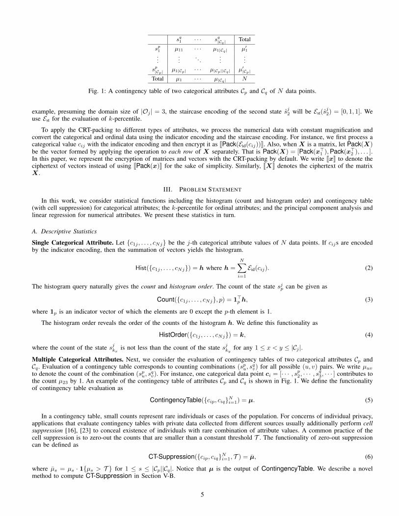
Fig. 1: A contingency table of two categorical attributes Cp and Cq of N data points.
example, presuming the domain size of |Oj | = 3, the staircase encoding of the second state sj2 will be Est(sj2) = [0, 1, 1]. We
use Est for the evaluation of k-percentile.
To apply the CRT-packing to different types of attributes, we process the numerical data with constant magnification andconvert the categorical and ordinal data using the indicator encoding and the staircase encoding. For instance, we first process acategorical value cij with the indicator encoding and then encrypt it as JPack(Eid(cij))K. Also, when X is a matrix, let Pack(X)be the vector formed by applying the operation to each row of X separately. That is Pack(X) = [Pack(x>1 ),Pack(x>2 ), . . . ].In this paper, we represent the encryption of matrices and vectors with the CRT-packing by default. We write JxK to denote theciphertext of vectors instead of using JPack(x)K for the sake of simplicity. Similarly, JXK denotes the ciphertext of the matrixX .
III. PROBLEM STATEMENT
In this work, we consider statistical functions including the histogram (count and histogram order) and contingency table(with cell suppression) for categorical attributes; the k-percentile for ordinal attributes; and the principal component analysis andlinear regression for numerical attributes. We present these statistics in turn.
A. Descriptive Statistics
Single Categorical Attribute. Let {c1j , . . . , cNj} be the j-th categorical attribute values of N data points. If cijs are encodedby the indicator encoding, then the summation of vectors yields the histogram.
Hist({c1j , . . . , cNj}) = h where h =
N∑i=1
Eid(cij). (2)
The histogram query naturally gives the count and histogram order. The count of the state sjp can be given as
Count({c1j , . . . , cNj}, p) = 1>p h, (3)
where 1p is an indicator vector of which the elements are 0 except the p-th element is 1.
The histogram order reveals the order of the counts of the histogram h. We define this functionality as
HistOrder({c1j , . . . , cNj}) = k, (4)
where the count of the state sjkx is not less than the count of the state sjky for any 1 ≤ x < y ≤ |Cj |.
Multiple Categorical Attributes. Next, we consider the evaluation of contingency tables of two categorical attributes Cp andCq . Evaluation of a contingency table corresponds to counting combinations (spu, s
qv) for all possible (u, v) pairs. We write µuv
to denote the count of the combination (spu, sqv). For instance, one categorical data point ci = [· · · , sp2, · · · , s
q3, · · · ] contributes to
the count µ23 by 1. An example of the contingency table of attributes Cp and Cq is shown in Fig. 1. We define the functionalityof contingency table evaluation as
ContingencyTable({cip, ciq}Ni=1) = µ. (5)
In a contingency table, small counts represent rare individuals or cases of the population. For concerns of individual privacy,applications that evaluate contingency tables with private data collected from different sources usually additionally perform cellsuppression [16], [23] to conceal existence of individuals with rare combination of attribute values. A common practice of thecell suppression is to zero-out the counts that are smaller than a constant threshold T . The functionality of zero-out suppressioncan be defined as
CT-Suppression({cip, ciq}Ni=1, T ) = µ, (6)
where µs = µs · 1{µs > T } for 1 ≤ s ≤ |Cp||Cq|. Notice that µ is the output of ContingencyTable. We describe a novelmethod to compute CT-Suppression in Section V-B.
5
Ordinal Attributes. For the ordinal attributes, we consider k-percentile. k-percentile is the value that separates given ordinalvalues into two parts so that the one part with lower values contains k % of the data. For instance, the 50-percentile is alsonamed as the median. Letting {o1j , . . . , oNj} be the j-th ordinal attribute values of N data points, we can sort the ordinal valuesin ascending order as oπ(1)j � · · · � oπ(N)j . Here, π is a permutation function that returns indices in descending order. Usingthe notation of π, we can define the k-percentile functionality as
k-Percentile(o1j , . . . , oNj) = oN∗j , (7)
where N∗ := π(d(k ·N)/100e) and oπ(i)j � oπ(i+1)j holds for all 1 ≤ i < N .
B. Predictive Statistics
Principal Component Analysis. PCA is a statistical procedure that converts a set of numerical observations of possibly correlatedvariables into a small number of directions that are mutually linearly independent. In PCA, we firstly compute a covariancematrix
Σ =1
NX>X − µµ> where µ =
1
N
N∑i=1
x>i . (8)
Then we compute the eigenvalues and eigenvectors of Σ. Let the eigenvalues of Σ be λ1 ≥ · · · ≥ λdn , and denote thecorresponding eigenvectors as u1, . . . ,udn . An iterative algorithm (i.e., PowerMethod) can evaluate the k-th eigenvalue λk andthe corresponding principal component uk with T iterations.
PowerMethod (Σ, {λq}k−1q=1 , {uq}
k−1q=1 ):
1. Σk := Σ−∑k−1q=1 λququ
>q .
2. Choose a random vector v(0) $← Zdnt .
3. For 0 ≤ τ < T , computev(τ+1) = Σkv
(τ). (9)
4. Output uk =v(T )
‖v(T )‖and λk =
‖v(T )‖‖v(T−1)‖
.
Linear Regression. The problem of linear regression is to find a model that predicts values of a numerical target variable fromobservations of numerical input variables using a linear equation. Let {(x>i , yi)}Ni=1 be the given dataset in which x>i are theinput variables and yi is the target variables. The model of linear regression is given as y ≈ x>w. Therein, the model w isobtained by minimizing the least-squares error:
w∗ = arg minw
1
N
N∑i=1
‖yi − x>i w‖22.
The analytical solution w∗ is given asw∗ = (X>X)−1X>y, (10)
where the matrix X and vector y are the collections of numerical data. The Eq. 10 is immediately solved if we can evaluate theinverse of X>X . We leverage a division-free variant of the iterative matrix inversion method from [13] so that we can computethe matrix inversion on FHE encrypted matrices. Let M be a matrix, λ be a real value, and T be the number of iterations. Thedivision-free matrix inversion method works as follows.
DF-MatrixInversion (M , λ, T ):
1. Initialize A(0) = M ,R(0) = I, α(0) = λ.
2. For 0 ≤ τ < T , compute
R(τ+1) = 2α(τ)R(τ) −R(τ)A(τ),
A(τ+1) = 2α(τ)A(τ) −A(τ)A(τ),
α(τ+1) = α(τ)α(τ).
(11)
3. Output R(T ).
Here I is an identity matrix. This method approximates the inverse of the matrix M . According to the analysis of [13], R(τ)
converges to λ2τM−1 quadratically if λ is close to the largest eigenvalue of M .
6
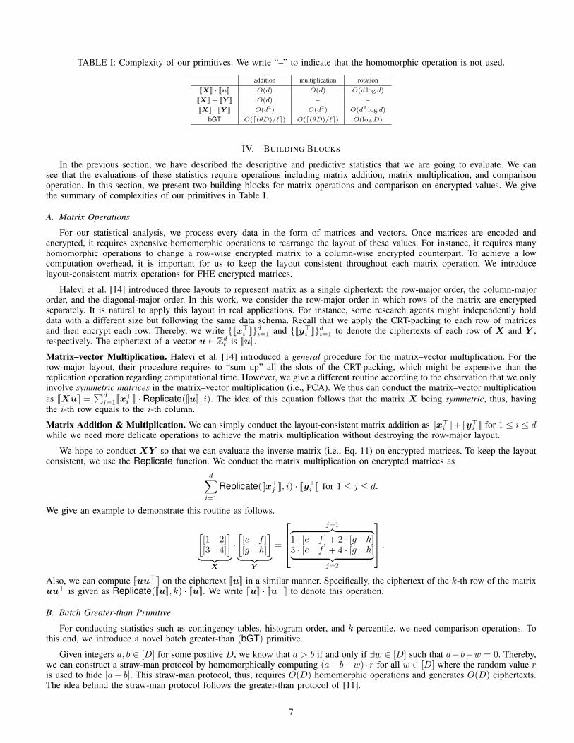
TABLE I: Complexity of our primitives. We write “–” to indicate that the homomorphic operation is not used.
addition multiplication rotation
JXK · JuK O(d) O(d) O(d log d)
JXK + JY K O(d) – –JXK · JY K O(d2) O(d2) O(d2 log d)
bGT O(d(θD)/`e) O(d(θD)/`e) O(logD)
IV. BUILDING BLOCKS
In the previous section, we have described the descriptive and predictive statistics that we are going to evaluate. We cansee that the evaluations of these statistics require operations including matrix addition, matrix multiplication, and comparisonoperation. In this section, we present two building blocks for matrix operations and comparison on encrypted values. We givethe summary of complexities of our primitives in Table I.
A. Matrix Operations
For our statistical analysis, we process every data in the form of matrices and vectors. Once matrices are encoded andencrypted, it requires expensive homomorphic operations to rearrange the layout of these values. For instance, it requires manyhomomorphic operations to change a row-wise encrypted matrix to a column-wise encrypted counterpart. To achieve a lowcomputation overhead, it is important for us to keep the layout consistent throughout each matrix operation. We introducelayout-consistent matrix operations for FHE encrypted matrices.
Halevi et al. [14] introduced three layouts to represent matrix as a single ciphertext: the row-major order, the column-majororder, and the diagonal-major order. In this work, we consider the row-major order in which rows of the matrix are encryptedseparately. It is natural to apply this layout in real applications. For instance, some research agents might independently holddata with a different size but following the same data schema. Recall that we apply the CRT-packing to each row of matricesand then encrypt each row. Thereby, we write {Jx>i K}di=1 and {Jy>i K}di=1 to denote the ciphertexts of each row of X and Y ,respectively. The ciphertext of a vector u ∈ Zdt is JuK.
Matrix–vector Multiplication. Halevi et al. [14] introduced a general procedure for the matrix–vector multiplication. For therow-major layout, their procedure requires to “sum up” all the slots of the CRT-packing, which might be expensive than thereplication operation regarding computational time. However, we give a different routine according to the observation that we onlyinvolve symmetric matrices in the matrix–vector multiplication (i.e., PCA). We thus can conduct the matrix–vector multiplicationas JXuK =
∑di=1Jx
>i K · Replicate(JuK, i). The idea of this equation follows that the matrix X being symmetric, thus, having
the i-th row equals to the i-th column.
Matrix Addition & Multiplication. We can simply conduct the layout-consistent matrix addition as Jx>i K+ Jy>i K for 1 ≤ i ≤ dwhile we need more delicate operations to achieve the matrix multiplication without destroying the row-major layout.
We hope to conduct XY so that we can evaluate the inverse matrix (i.e., Eq. 11) on encrypted matrices. To keep the layoutconsistent, we use the Replicate function. We conduct the matrix multiplication on encrypted matrices as
d∑i=1
Replicate(Jx>j K, i) · Jy>i K for 1 ≤ j ≤ d.
We give an example to demonstrate this routine as follows.
[[1 2][3 4]
]︸ ︷︷ ︸
X
·[[e f ][g h]
]︸ ︷︷ ︸
Y
=
j=1︷ ︸︸ ︷
1 · [e f ] + 2 · [g h]3 · [e f ] + 4 · [g h]︸ ︷︷ ︸
j=2
.Also, we can compute Juu>K on the ciphertext JuK in a similar manner. Specifically, the ciphertext of the k-th row of the matrixuu> is given as Replicate(JuK, k) · JuK. We write JuK · Ju>K to denote this operation.
B. Batch Greater-than Primitive
For conducting statistics such as contingency tables, histogram order, and k-percentile, we need comparison operations. Tothis end, we introduce a novel batch greater-than (bGT) primitive.
Given integers a, b ∈ [D] for some positive D, we know that a > b if and only if ∃w ∈ [D] such that a−b−w = 0. Thereby,we can construct a straw-man protocol by homomorphically computing (a− b−w) · r for all w ∈ [D] where the random value ris used to hide |a− b|. This straw-man protocol, thus, requires O(D) homomorphic operations and generates O(D) ciphertexts.The idea behind the straw-man protocol follows the greater-than protocol of [11].
7
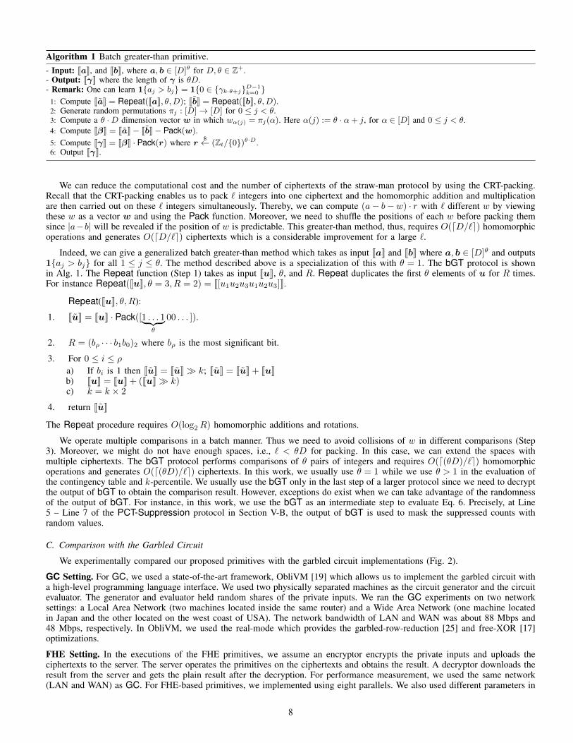
Algorithm 1 Batch greater-than primitive.- Input: JaK, and JbK, where a, b ∈ [D]θ for D, θ ∈ Z+.- Output: JγK where the length of γ is θD.- Remark: One can learn 1{aj > bj} = 1{0 ∈ {γk·θ+j}D−1
k=0 }1: Compute JaK = Repeat(JaK, θ,D); JbK = Repeat(JbK, θ,D).2: Generate random permutations πj : [D]→ [D] for 0 ≤ j < θ.3: Compute a θ ·D dimension vector w in which wα(j) = πj(α). Here α(j) := θ · α+ j, for α ∈ [D] and 0 ≤ j < θ.4: Compute JβK = JaK− JbK− Pack(w).5: Compute JγK = JβK · Pack(r) where r $← (Zt/{0})θ·D .6: Output JγK.
We can reduce the computational cost and the number of ciphertexts of the straw-man protocol by using the CRT-packing.Recall that the CRT-packing enables us to pack ` integers into one ciphertext and the homomorphic addition and multiplicationare then carried out on these ` integers simultaneously. Thereby, we can compute (a− b−w) · r with ` different w by viewingthese w as a vector w and using the Pack function. Moreover, we need to shuffle the positions of each w before packing themsince |a−b| will be revealed if the position of w is predictable. This greater-than method, thus, requires O(dD/`e) homomorphicoperations and generates O(dD/`e) ciphertexts which is a considerable improvement for a large `.
Indeed, we can give a generalized batch greater-than method which takes as input JaK and JbK where a, b ∈ [D]θ and outputs1{aj > bj} for all 1 ≤ j ≤ θ. The method described above is a specialization of this with θ = 1. The bGT protocol is shownin Alg. 1. The Repeat function (Step 1) takes as input JuK, θ, and R. Repeat duplicates the first θ elements of u for R times.For instance Repeat(JuK, θ = 3, R = 2) = J[u1u2u3u1u2u3]K.
Repeat(JuK, θ, R):
1. JuK = JuK · Pack([1 . . . 1︸ ︷︷ ︸θ
00 . . . ]).
2. R = (bρ · · · b1b0)2 where bρ is the most significant bit.
3. For 0 ≤ i ≤ ρa) If bi is 1 then JuK = JuK� k; JuK = JuK + JuKb) JuK = JuK + (JuK� k)c) k = k × 2
4. return JuK
The Repeat procedure requires O(log2R) homomorphic additions and rotations.
We operate multiple comparisons in a batch manner. Thus we need to avoid collisions of w in different comparisons (Step3). Moreover, we might do not have enough spaces, i.e., ` < θD for packing. In this case, we can extend the spaces withmultiple ciphertexts. The bGT protocol performs comparisons of θ pairs of integers and requires O(d(θD)/`e) homomorphicoperations and generates O(d(θD)/`e) ciphertexts. In this work, we usually use θ = 1 while we use θ > 1 in the evaluation ofthe contingency table and k-percentile. We usually use the bGT only in the last step of a larger protocol since we need to decryptthe output of bGT to obtain the comparison result. However, exceptions do exist when we can take advantage of the randomnessof the output of bGT. For instance, in this work, we use the bGT as an intermediate step to evaluate Eq. 6. Precisely, at Line5 – Line 7 of the PCT-Suppression protocol in Section V-B, the output of bGT is used to mask the suppressed counts withrandom values.
C. Comparison with the Garbled Circuit
We experimentally compared our proposed primitives with the garbled circuit implementations (Fig. 2).
GC Setting. For GC, we used a state-of-the-art framework, ObliVM [19] which allows us to implement the garbled circuit witha high-level programming language interface. We used two physically separated machines as the circuit generator and the circuitevaluator. The generator and evaluator held random shares of the private inputs. We ran the GC experiments on two networksettings: a Local Area Network (two machines located inside the same router) and a Wide Area Network (one machine locatedin Japan and the other located on the west coast of USA). The network bandwidth of LAN and WAN was about 88 Mbps and48 Mbps, respectively. In ObliVM, we used the real-mode which provides the garbled-row-reduction [25] and free-XOR [17]optimizations.
FHE Setting. In the executions of the FHE primitives, we assume an encryptor encrypts the private inputs and uploads theciphertexts to the server. The server operates the primitives on the ciphertexts and obtains the result. A decryptor downloads theresult from the server and gets the plain result after the decryption. For performance measurement, we used the same network(LAN and WAN) as GC. For FHE-based primitives, we implemented using eight parallels. We also used different parameters in
8
0.01
0.1
1
10
100
4 8 12 16 20 24
Seco
nd
#Bits
GC-LAN
GC-WAN
FHE
(a) Evaluation Time of GT
0.001
0.01
0.1
1
10
100
2 4 8 16 32 64
Seco
nd
Matrix Dimension
GC-LAN
GC-WAN
FHE
(b) Evaluation Time of X + Y
0.1
1
10
100
1000
10000
2 4 8 16 32 64
Seco
nd
Matrix Dimension
GC-LAN
GC-WAN
FHE
(c) Evaluation Time of XY
0.001
0.01
0.1
1
10
100
1000
10000
4 8 12 16 20 24
MB
#Bits
GC
76 88 100 112 124 136
FHE
(d) Ciphertext Size of GT
0.001
0.01
0.1
1
10
100
1000
10000
2 4 8 16 32 64
MB
Matrix Dimension
GC
384
1536
6144
24576
98304
393216
FHE
(e) Ciphertext Size of X + Y
0.1
1
10
100
1000
10000
100000
2 4 8 16 32 64
MB
Matrix Dimension
GC
16640
132096
1052672
8404992
67174400
537133056
FHE
(f) Ciphertext Size of XY
0.1
1
10
100
1000
4 8 12 16 20 24
Seco
nd
#Bits
FHE-LAN
FHE-WAN
GC-LAN
GC-WAN
(g) Operation Time of GT
0.1
1
10
100
2 4 8 16 32 64
Seco
nd
#Matrix Dimension
FHE-LAN
FHE-WAN
GC-LAN
GC-WAN
(h) Operation Time of X + Y
0.1
1
10
100
1000
10000
2 4 8 16 32 64
Seco
nd
#Matrix Dimension
FHE-LAN
FHE-WAN
GC-LAN
GC-WAN
(i) Operation Time of XY
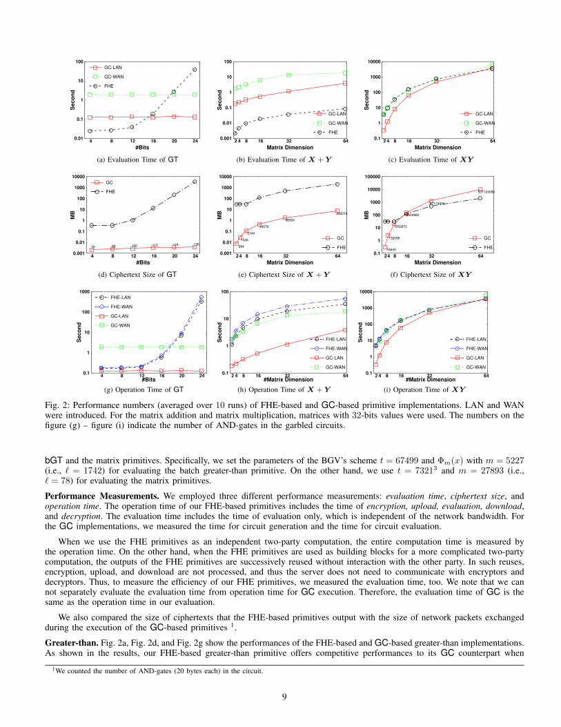
Fig. 2: Performance numbers (averaged over 10 runs) of FHE-based and GC-based primitive implementations. LAN and WANwere introduced. For the matrix addition and matrix multiplication, matrices with 32-bits values were used. The numbers on thefigure (g) – figure (i) indicate the number of AND-gates in the garbled circuits.
bGT and the matrix primitives. Specifically, we set the parameters of the BGV’s scheme t = 67499 and Φm(x) with m = 5227(i.e., ` = 1742) for evaluating the batch greater-than primitive. On the other hand, we use t = 73213 and m = 27893 (i.e.,` = 78) for evaluating the matrix primitives.
Performance Measurements. We employed three different performance measurements: evaluation time, ciphertext size, andoperation time. The operation time of our FHE-based primitives includes the time of encryption, upload, evaluation, download,and decryption. The evaluation time includes the time of evaluation only, which is independent of the network bandwidth. Forthe GC implementations, we measured the time for circuit generation and the time for circuit evaluation.
When we use the FHE primitives as an independent two-party computation, the entire computation time is measured bythe operation time. On the other hand, when the FHE primitives are used as building blocks for a more complicated two-partycomputation, the outputs of the FHE primitives are successively reused without interaction with the other party. In such reuses,encryption, upload, and download are not processed, and thus the server does not need to communicate with encryptors anddecryptors. Thus, to measure the efficiency of our FHE primitives, we measured the evaluation time, too. We note that we cannot separately evaluate the evaluation time from operation time for GC execution. Therefore, the evaluation time of GC is thesame as the operation time in our evaluation.
We also compared the size of ciphertexts that the FHE-based primitives output with the size of network packets exchangedduring the execution of the GC-based primitives 1.
Greater-than. Fig. 2a, Fig. 2d, and Fig. 2g show the performances of the FHE-based and GC-based greater-than implementations.As shown in the results, our FHE-based greater-than primitive offers competitive performances to its GC counterpart when
1We counted the number of AND-gates (20 bytes each) in the circuit.
9
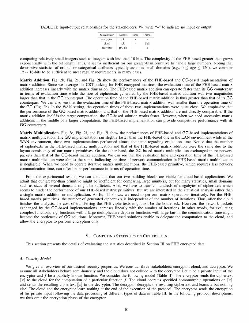
TABLE II: Input-output relationships for the stakeholders. We write “–” to indicate no input or output.
Stakeholder Possess Input Output
encryptor pk x –cloud pk – JzK
decryptor pk, sk – z
comparing relatively small integers such as integers with less than 16 bits. The complexity of the FHE-based greater-than growsexponentially with the bit length. Thus, it seems inefficient for our greater-than primitive to handle large numbers. Noting thatdescriptive statistics of ordinal or categorical attributes typically assumes small domains (e.g., 0 ≤ age ≤ 150), we consider12 ∼ 16-bits to be sufficient to meet regular requirements in many cases.
Matrix Addition. Fig. 2b, Fig. 2e, and Fig. 2h show the performances of the FHE-based and GC-based implementations ofmatrix addition. Since we leverage the CRT-packing for FHE encrypted matrices, the evaluation time of the FHE-based matrixaddition increases linearly with the matrix dimension. The FHE-based matrix addition can operate faster than its GC counterpartin terms of evaluation time while the size of ciphertexts generated by the FHE-based matrix addition was two magnitudeslarger than that in the GC counterpart. The operation time of the FHE-based matrix addition is thus greater than that of its GCcounterpart. We can also see that the evaluation time of the FHE-based matrix addition was smaller than the operation time ofthe GC (Fig. 2b). In the WAN setting, the operation times of these two implementations were quite close. We emphasize thatthe performance of the GC-based matrix addition and that of the FHE-based matrix addition are not directly comparable. If thematrix addition itself is the target computation, the GC-based solution works faster. However, when we need successive matrixadditions in the middle of a larger computation, the FHE-based implementation can provide competitive performance with itsGC counterpart.
Matrix Multiplication. Fig. 2c, Fig. 2f, and Fig. 2i show the performances of FHE-based and GC-based implementations ofmatrix multiplication. The GC implementation ran slightly faster than the FHE-based one in the LAN environment while in theWAN environment, these two implementations performed almost the same regarding evaluation time. Notice that the numberof ciphertexts in the FHE-based matrix multiplication and that of the FHE-based matrix addition were the same due to thelayout-consistency of our matrix primitives. On the other hand, the GC-based matrix multiplication exchanged more networkpackets than that of the GC-based matrix addition. We can see that the evaluation time and operation time of the FHE-basedmatrix multiplication were almost the same, indicating the time of network communication in FHE-based matrix multiplicationis negligible. When we need to operate iterative matrix multiplications, the FHE-based primitive, which requires less networkcommunication time, can offer better performance in terms of operation time.
From the experimental results, we can conclude that our two building blocks are viable for cloud-based applications. Weadmit that our greater-than primitive might be inefficient for comparing large numbers, but for many statistics, small domainssuch as sizes of several thousand might be sufficient. Also, we have to transfer hundreds of megabytes of ciphertexts whichseems to hinder the performance of our FHE-based matrix primitives. But we are interested in the statistical analysis rather thana single matrix addition or multiplication. As Eq. 11 shows, we need to perform matrix operations iteratively. For the FHE-based matrix primitives, the number of generated ciphertexts is independent of the number of iterations. Thus, after the cloudfinishes the analysis, the cost of transferring the FHE ciphertexts might not be the bottleneck. However, the network packetsexchanged by the GC-based implementations increases linearly with the number of iterations. In other words, for evaluatingcomplex functions, e.g. functions with a large multiplicative depth or functions with large fan-in, the communication time mightbecome the bottleneck of GC solutions. Moreover, FHE-based solutions enable to delegate the computation to the cloud, andallow the encryptor to perform encryption only.
V. COMPUTING STATISTICS ON CIPHERTEXTS
This section presents the details of evaluating the statistics described in Section III on FHE encrypted data.
A. Security Model
We give an overview of our desired security properties. We consider three stakeholders: encryptor, cloud, and decryptor. Weassume all stakeholders behave semi-honestly and the cloud does not collude with the decryptor. Let x be a private input of theencryptor and f be a publicly known function. We consider the following model (Table II). The encryptor sends the ciphertextJxK to the cloud for the computation of a particular function f . The cloud operates specified homomorphic operations on JxKand sends the resulting ciphertext JzK to the decryptor. The decryptor decrypts the resulting ciphertext and learns z but nothingelse. The cloud and the encryptor learn nothing at the end of the execution of the protocol. The encryptor sends the encryptionof his private input following the data processing of different types of data in Table III. In the following protocol descriptions,we thus omit the encryption phase of the encryptor.
10
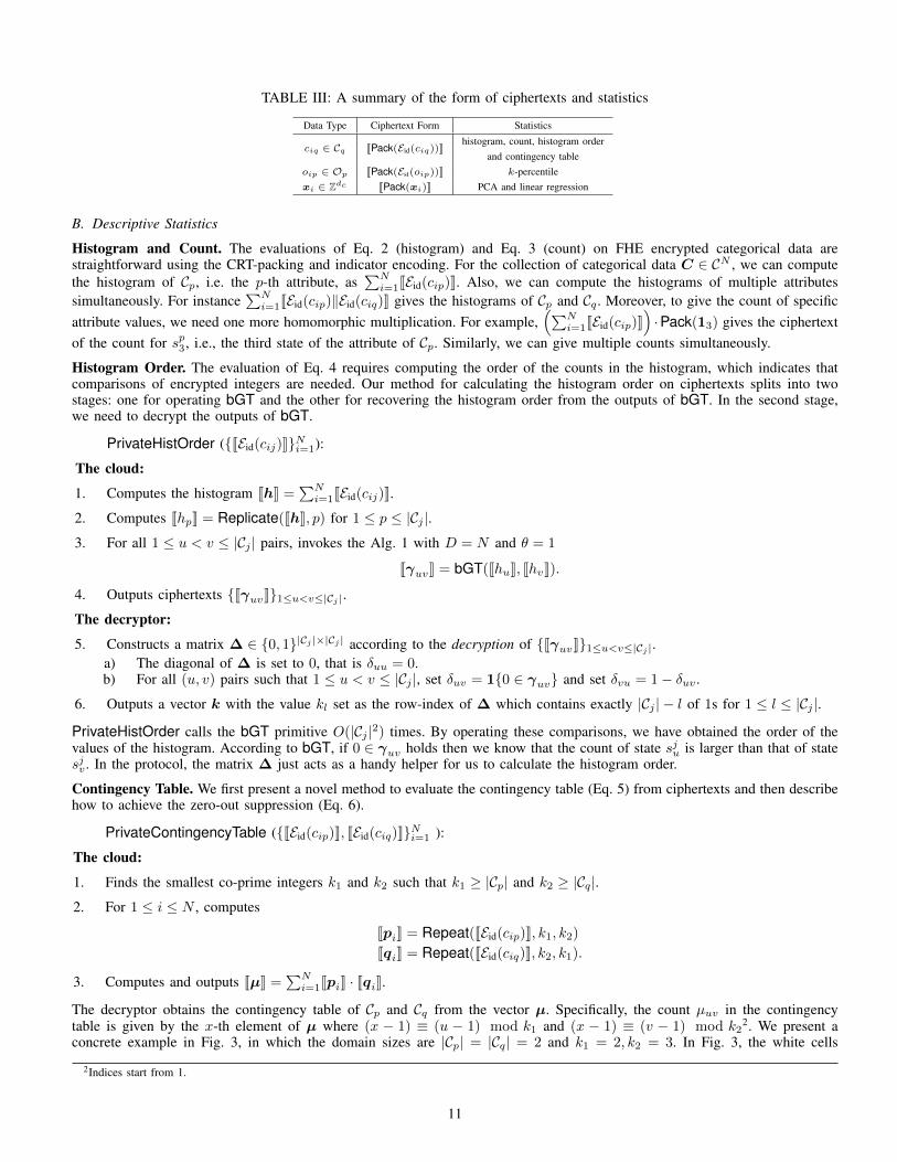
TABLE III: A summary of the form of ciphertexts and statistics
Data Type Ciphertext Form Statistics
ciq ∈ Cq JPack(Eid(ciq))Khistogram, count, histogram order
and contingency tableoip ∈ Op JPack(Est(oip))K k-percentilexi ∈ Zdc JPack(xi)K PCA and linear regression
B. Descriptive Statistics
Histogram and Count. The evaluations of Eq. 2 (histogram) and Eq. 3 (count) on FHE encrypted categorical data arestraightforward using the CRT-packing and indicator encoding. For the collection of categorical data C ∈ CN , we can computethe histogram of Cp, i.e. the p-th attribute, as
∑Ni=1JEid(cip)K. Also, we can compute the histograms of multiple attributes
simultaneously. For instance∑Ni=1JEid(cip)‖Eid(ciq)K gives the histograms of Cp and Cq . Moreover, to give the count of specific
attribute values, we need one more homomorphic multiplication. For example,(∑N
i=1JEid(cip)K)·Pack(13) gives the ciphertext
of the count for sp3, i.e., the third state of the attribute of Cp. Similarly, we can give multiple counts simultaneously.
Histogram Order. The evaluation of Eq. 4 requires computing the order of the counts in the histogram, which indicates thatcomparisons of encrypted integers are needed. Our method for calculating the histogram order on ciphertexts splits into twostages: one for operating bGT and the other for recovering the histogram order from the outputs of bGT. In the second stage,we need to decrypt the outputs of bGT.
PrivateHistOrder ({JEid(cij)K}Ni=1):
The cloud:
1. Computes the histogram JhK =∑Ni=1JEid(cij)K.
2. Computes JhpK = Replicate(JhK, p) for 1 ≤ p ≤ |Cj |.3. For all 1 ≤ u < v ≤ |Cj | pairs, invokes the Alg. 1 with D = N and θ = 1
JγuvK = bGT(JhuK, JhvK).
4. Outputs ciphertexts {JγuvK}1≤u<v≤|Cj |.The decryptor:
5. Constructs a matrix ∆ ∈ {0, 1}|Cj |×|Cj | according to the decryption of {JγuvK}1≤u<v≤|Cj |.a) The diagonal of ∆ is set to 0, that is δuu = 0.b) For all (u, v) pairs such that 1 ≤ u < v ≤ |Cj |, set δuv = 1{0 ∈ γuv} and set δvu = 1− δuv .
6. Outputs a vector k with the value kl set as the row-index of ∆ which contains exactly |Cj | − l of 1s for 1 ≤ l ≤ |Cj |.
PrivateHistOrder calls the bGT primitive O(|Cj |2) times. By operating these comparisons, we have obtained the order of thevalues of the histogram. According to bGT, if 0 ∈ γuv holds then we know that the count of state sju is larger than that of statesjv . In the protocol, the matrix ∆ just acts as a handy helper for us to calculate the histogram order.
Contingency Table. We first present a novel method to evaluate the contingency table (Eq. 5) from ciphertexts and then describehow to achieve the zero-out suppression (Eq. 6).
PrivateContingencyTable ({JEid(cip)K, JEid(ciq)K}Ni=1 ):
The cloud:
1. Finds the smallest co-prime integers k1 and k2 such that k1 ≥ |Cp| and k2 ≥ |Cq|.2. For 1 ≤ i ≤ N , computes
JpiK = Repeat(JEid(cip)K, k1, k2)
JqiK = Repeat(JEid(ciq)K, k2, k1).
3. Computes and outputs JµK =∑Ni=1JpiK · JqiK.
The decryptor obtains the contingency table of Cp and Cq from the vector µ. Specifically, the count µuv in the contingencytable is given by the x-th element of µ where (x − 1) ≡ (u − 1) mod k1 and (x − 1) ≡ (v − 1) mod k2
2. We present aconcrete example in Fig. 3, in which the domain sizes are |Cp| = |Cq| = 2 and k1 = 2, k2 = 3. In Fig. 3, the white cells
2Indices start from 1.
11
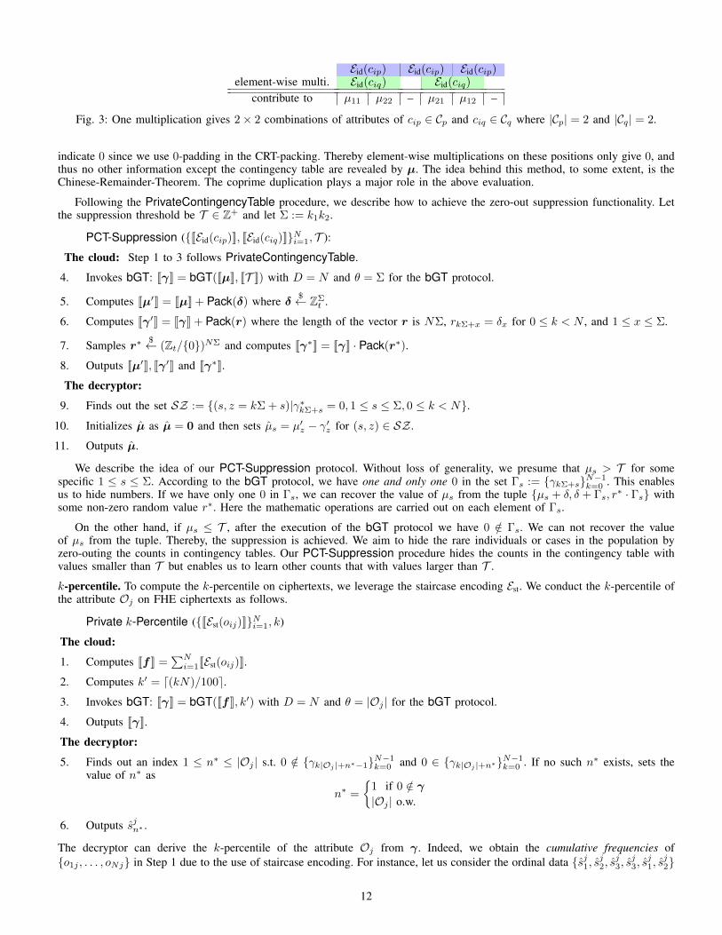
Eid(cip) Eid(cip) Eid(cip)element-wise multi. Eid(ciq) Eid(ciq)
contribute to µ11 µ22 – µ21 µ12 –
Fig. 3: One multiplication gives 2× 2 combinations of attributes of cip ∈ Cp and ciq ∈ Cq where |Cp| = 2 and |Cq| = 2.
indicate 0 since we use 0-padding in the CRT-packing. Thereby element-wise multiplications on these positions only give 0, andthus no other information except the contingency table are revealed by µ. The idea behind this method, to some extent, is theChinese-Remainder-Theorem. The coprime duplication plays a major role in the above evaluation.
Following the PrivateContingencyTable procedure, we describe how to achieve the zero-out suppression functionality. Letthe suppression threshold be T ∈ Z+ and let Σ := k1k2.
PCT-Suppression ({JEid(cip)K, JEid(ciq)K}Ni=1, T ):
The cloud: Step 1 to 3 follows PrivateContingencyTable.
4. Invokes bGT: JγK = bGT(JµK, JT K) with D = N and θ = Σ for the bGT protocol.
5. Computes Jµ′K = JµK + Pack(δ) where δ $← ZΣt .
6. Computes Jγ′K = JγK + Pack(r) where the length of the vector r is NΣ, rkΣ+x = δx for 0 ≤ k < N , and 1 ≤ x ≤ Σ.
7. Samples r∗ $← (Zt/{0})NΣ and computes Jγ∗K = JγK · Pack(r∗).
8. Outputs Jµ′K, Jγ′K and Jγ∗K.
The decryptor:
9. Finds out the set SZ := {(s, z = kΣ + s)|γ∗kΣ+s = 0, 1 ≤ s ≤ Σ, 0 ≤ k < N}.
10. Initializes µ as µ = 0 and then sets µs = µ′z − γ′z for (s, z) ∈ SZ .
11. Outputs µ.
We describe the idea of our PCT-Suppression protocol. Without loss of generality, we presume that µs > T for somespecific 1 ≤ s ≤ Σ. According to the bGT protocol, we have one and only one 0 in the set Γs := {γkΣ+s}N−1
k=0 . This enablesus to hide numbers. If we have only one 0 in Γs, we can recover the value of µs from the tuple {µs + δ, δ + Γs, r
∗ · Γs} withsome non-zero random value r∗. Here the mathematic operations are carried out on each element of Γs.
On the other hand, if µs ≤ T , after the execution of the bGT protocol we have 0 /∈ Γs. We can not recover the valueof µs from the tuple. Thereby, the suppression is achieved. We aim to hide the rare individuals or cases in the population byzero-outing the counts in contingency tables. Our PCT-Suppression procedure hides the counts in the contingency table withvalues smaller than T but enables us to learn other counts that with values larger than T .
k-percentile. To compute the k-percentile on ciphertexts, we leverage the staircase encoding Est. We conduct the k-percentile ofthe attribute Oj on FHE ciphertexts as follows.
Private k-Percentile ({JEst(oij)K}Ni=1, k)
The cloud:
1. Computes JfK =∑Ni=1JEst(oij)K.
2. Computes k′ = d(kN)/100e.3. Invokes bGT: JγK = bGT(JfK, k′) with D = N and θ = |Oj | for the bGT protocol.
4. Outputs JγK.
The decryptor:
5. Finds out an index 1 ≤ n∗ ≤ |Oj | s.t. 0 /∈ {γk|Oj |+n∗−1}N−1k=0 and 0 ∈ {γk|Oj |+n∗}
N−1k=0 . If no such n∗ exists, sets the
value of n∗ as
n∗ =
{1 if 0 /∈ γ|Oj | o.w.
6. Outputs sjn∗ .
The decryptor can derive the k-percentile of the attribute Oj from γ. Indeed, we obtain the cumulative frequencies of{o1j , . . . , oNj} in Step 1 due to the use of staircase encoding. For instance, let us consider the ordinal data {sj1, s
j2, s
j3, s
j3, s
j1, s
j2}
12
for N = 6. Then the summation in Step 1 gives cumulative frequencies f = [2, 4, 6]. To get the k-percentile, we only need to findout, from left to right, the first frequency that is larger than d(kN)/100e. In the previous example, we know sj2 is the 50-percentilepoint because f1 < 3 ∧ f2 ≥ 3. We perform the comparisons using the bGT protocol. Thus, to determine the k-percentile fromγ we simply find an index 1 ≤ n∗ ≤ |Oj | s.t. 0 /∈ {γk|Oj |+n∗−1}N−1
k=0 while 0 ∈ {γk|Oj |+n∗}N−1k=0 . For the boundary conditions,
we can determine that sj1 is the k-percentile point if 0 is absent in γ. On the other hand if 0 ∈ {γk|Oj |+n∗}N−1k=0 for all possible
n∗, we know that sj|Oj | is the k-percentile of the population.
C. Predictive Statistics
Principal Component Analysis. For the evaluation of PCA, we can perform the computation of Eq. 8 and Eq. 9 on ciphertextsdirectly. Given the collection of numerical data X ∈ ZN×dnt , we evaluate the first principal component with T iterations asfollows.
PrivatePCA ({Jx>i K, Jxix>i K}Ni=1, T )
The cloud:
1. Computes JNµK =∑Ni=1Jx
>i K.
2. Computes JN2ΣK = N ·∑Ni=1Jxix
>i K− JNµK · JNµ>K.
3. Computes Jv(τ+1)K = JN2ΣK · Jv(τ)K for 0 ≤ τ < T .
4. Outputs Jv(T )K and Jv(T−1)K.
5. The decryptor outputs the largest eigenvalue as λ1 = ‖v(T )‖/‖v(T−1)‖ and the associated eigenvector as u1 =v(T )/‖v(T )‖.
Step 1 and Step 2 follow Eq. 8 except we can not perform the division on ciphertexts. Notice that, in Step 2, the operationJNµK · JNµ>K generates ciphertexts of a matrix. The evaluation in Step 3 is also straightforward using our matrix–vectormultiplication primitives described in Section IV-A.
Linear Regression. To conduct the linear regression of Eq. 10, we need to compute the inverse of the design matrix X>X .To do so, we use the DF-MatrixInversion procedure in Eq. 11. The evaluation of Eq. 11 on ciphertexts are straightforwardusing our matrix multiplication primitive described in Section IV-A. Given the collection of numerical data {(x>i , yi)}Ni=1 andthe largest eigenvalue λ1 of the design matrix, we can evaluate Eq. 10 with T iterations as follows.
PrivateLR ({Jyix>i K, Jxix>i K}Ni=1, Jλ1K, T )
The cloud:
1. Computes JX>yK =∑Ni=1Jyix
>i K and JX>XK =
∑Ni=1Jxix
>i K.
2. Invokes the DF-MatrixInversion procedure
Jλ2T
1 (X>X)−1K = DF-MatrixInversion(JX>XK, Jλ1K, T ).
3. Outputs Jλ2T
1 w∗K = Jλ2T
1 (X>X)−1K · JX>yK.
4. The decryptor outputs w∗ by dividing λ2T
1 w∗ with λ2T
1 .
Notice that the multiplication in Step 3 is a matrix–vector multiplication. The DF-MatrixInversion computes the matrix inversionwith a known factor λ2T
1 . Thereby, our PrivateLR procedure computes the linear regression model w∗ with the factor λ2T
1 .
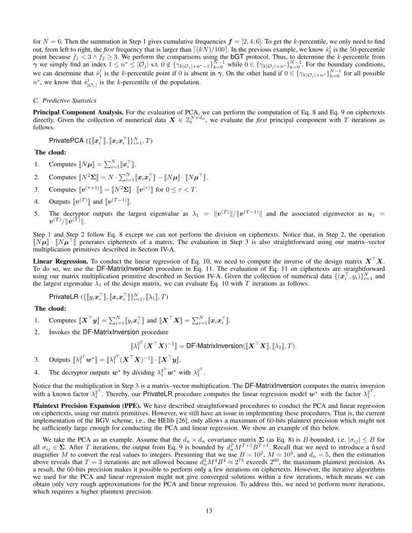
Plaintext Precision Expansion (PPE). We have described straightforward procedures to conduct the PCA and linear regressionon ciphertexts, using our matrix primitives. However, we still have an issue in implementing these procedures. That is, the currentimplementation of the BGV scheme, i.e., the HElib [26], only allows a maximum of 60-bits plaintext precision which might notbe sufficiently large enough for conducting the PCA and linear regression. We show an example of this below.
We take the PCA as an example. Assume that the dn × dn covariance matrix Σ (as Eq. 8) is B-bounded, i.e. |σij | ≤ B forall σij ∈ Σ. After T iterations, the output from Eq. 9 is bounded by dTnM
T+1BT+1. Recall that we need to introduce a fixedmagnifier M to convert the real values to integers. Presuming that we use B = 102, M = 103, and dn = 5, then the estimationabove reveals that T = 3 iterations are not allowed because d3
nM4B4 ≈ 273 exceeds 260, the maximum plaintext precision. As
a result, the 60-bits precision makes it possible to perform only a few iterations on ciphertexts. However, the iterative algorithmswe used for the PCA and linear regression might not give converged solutions within a few iterations, which means we canobtain only very rough approximations for the PCA and linear regression. To address this, we need to perform more iterations,which requires a higher plaintext precision.
13
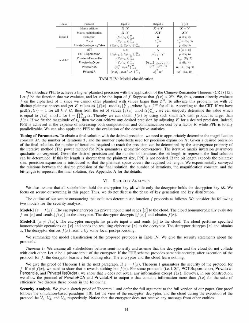
Class Protocol Input x Output z f(x)
model-I
Matrix addition X,Y X + Y X + Y
Matrix multiplication X,Y XY XY
Histogram {Eid(cij)}Ni=1 h h (Eq. 2)Count {Eid(cij)}Ni=1 1>p h 1>p h (Eq. 3)
PrivateContingencyTable {Eid(cpj), Eid(cqj)}Ni=1 µ µ (Eq. 5)
model-II
bGT a, b γ 1{a > b}PCT-Suppression {Eid(cpj), Eid(cqj)}Ni=1 µ′,γ′,γ∗ µ (Eq. 6)
Private k-Percentile {Est(oij)}Ni=1 γ sjn∗ (Eq. 7)
PrivateHistOrder {Eid(cij)}Ni=1 {γuv}1≤u<v≤|Cj | k (Eq. 4)
PrivatePCA {x>i ,xix>i }
Ni=1 v(T ),v(T−1) u1, λ1 (Eq. 9)
PrivateLR {yix>i ,xix>i , λ1}Ni=1 λ2T
1 w∗ w∗ (Eq. 10)
TABLE IV: Model classification
We introduce PPE to achieve a higher plaintext precision with the application of the Chinese-Remainder-Theorem (CRT) [15].Let f be the function that we evaluate, and let x be the input of f . Suppose that f(x) > 260. We, thus, cannot directly evaluatef on the ciphertext of x since we cannot offer plaintext with values larger than 260. To alleviate this problem, we with Kdistinct plaintext spaces and get K values as {f(x) mod tk}Kk=1, where tk < 260 for all k. According to the CRT, if we havegcd(tk, tk′) = 1 for all k 6= k′, then from the set of values {f(x) mod tk}Kk=1, we can uniquely determine the value whichis equal to f(x) mod t for t =
∏Kk=1 tk. Thereby we can obtain f(x) by using such small tk’s with product is larger than
f(x). If we fix the magnitude of tk, then we can achieve any desired precision by adjusting K for a desired precision. Indeed,PPE is achieved at the expense of increasing both computational and communication cost by a factor K while PPE is totallyparallelizable. We can also apply the PPE to the evaluation of the descriptive statistics.
Tuning of Parameters. To obtain a final solution with the desired precision, we need to appropriately determine the magnificationconstant M , the number of iterations T , and the number ciphertexts used for precision expansion K. Given a desired precisionof the final solution, the number of iterations required to reach the precision can be determined by the convergence property ofthe iterative method (The power method for PCA guarantees geometric convergence. The iterative matrix inversion guaranteesquadratic convergence). Given the desired precision and the number of iterations, the bit-length to represent the final solutioncan be determined. If this bit length is shorter than the plaintext size, PPE is not needed. If the bit length exceeds the plaintextsize, precision expansion is introduced so that the plaintext space covers the required bit length. We experimentally surveyedthe relations between the desired precision of the final solution, the number of iterations, the magnification constant, and thebit-length to represent the final solution. See Appendix A for the details.
VI. SECURITY ANALYSIS
We also assume that all stakeholders hold the encryption key pk while only the decryptor holds the decryption key sk. Wefocus on secure outsourcing in this paper. Thus, we do not discuss the phase of key generation and key distribution.
The outline of our secure outsourcing that evaluates deterministic function f proceeds as follows. We consider the followingtwo models for the security analysis.
Model-I (z = f(x)). The encryptor encrypts his private input x and sends JxK to the cloud. The cloud homomorphically evaluatesf on JxK and sends Jf(x)K to the decryptor. The decryptor decrypts Jf(x)K and obtains f(x).
Model-II (z 6= f(x)). The encryptor encrypts his private input x and sends JxK to the cloud. The cloud performs specifiedhomomorphic operations on JxK and sends the resulting ciphertext JzK to the decryptor. The decryptor decrypts JzK and obtainsz. The decryptor derives f(x) from z by some local post-processing.
We summarize the model classification of the proposed protocols in Table IV. We give the security statements about theprotocols.
Theorem 1: We assume all stakeholders behave semi-honestly and assume that the decryptor and the cloud do not colludewith each other. Let x be a private input of the encryptor. If the FHE scheme provides semantic security, after execution of theprotocol for f , the decryptor learns z but nothing else. The encryptor and the cloud learn nothing.
We give the proof of Theorem 1 in the next paragraph. If z = f(x), Theorem 1 guarantees the security of the protocol forf . If z 6= f(x), we need to show that z reveals nothing but f(x). For some protocols (i.e. bGT, PCT-Suppression, Private k-Percentile, and PrivateHistOrder), we show that z does not reveal any information except f(x). However, in our construction,we allow the protocol of PrivatePCA and PrivateLR to output z that contains information more than f(x) for the sake ofefficiency. We discuss these points in the following.
Security Analysis. We give a sketch proof of Theorem 1 and defer the full argument to the full version of our paper. Our prooffollows the simulation-based paradigm [10]. Let the view of the encryptor, decryptor, and the cloud during the execution of theprotocol be Ve, Vd, and Vc, respectively. Notice that the encryptor does not receive any message from other entities.
14
Proof of Theorem 1 (Sketch): Let pk be the encryption key used by the encryptor. From the construction of the protocol, thesecurity against the semi-honest encryptor and the semi-honest decryptor are apparent. So, we omit the proofs for the encryptorand decryptor.
Security against a semi-honest cloud follows from the fact that the view of the cloud, Vc, consists of {pk,Encpk(x),Encpk(z)}.We can simply construct a simulator Sc as follow. Sc firstly randomly chooses values x′ and z′. Then Sc simulates Vc byVc = {pk,Encpk(x′),Encpk(z′)}. Since the FHE provides semantic security by assumption, Vc and Vc are indistinguishable.Thus, our protocols are secure at the presence of a semi-honest cloud.
Security Discussion under Model-II. For protocols classified in the model-II, the decryptor obtains f(x) with some post-processing on z. We show that z reveals nothing except f(x) for certain protocols.
Batch Greater-Than. In bGT(JaK, JbK) (we assume that θ = 1), if a ≤ b holds then the output z consists of D uniform randomvalues from Zt/{0} and reveals nothing but the output. If a > b, we have one 0 in γ at a position selected randomly and valuesat remaining positions distribute uniformly on Zt/{0}. Thereby, from z the decryptor can only learn 1{a > b} but nothing else.
PCT-Suppression. We use bGT to compare Σ values in the contingency table, i.e., µ, with the threshold T . Since thesecomparisons are independent of each other, we focus on a specific µs. γ∗ is the output from the bGT (each element aremultiplied with non-zero random values). If µs > T , we have one 0 in set Γs := {γ∗kΣ+s}
N−1k=0 at a random position and
remaining values are all random. Otherwise, Γs consists of uniform random values on Zt/{0}. Presume that, in the set Γs, wehave γ∗k′Σ+s = 0. Then the decryptor can learn µs = µ′s − γ′k′ which is the desired output. On the other hand if µs ≤ T , forall 1 ≤ k ≤ Σ, value µ′s − γ′k is uniformly distributed on Zt/{0}. Consequently, from the output z, the decryptor only learns µand nothing else.
Private k-Percentile. The output z of the k-percentile protocol comes from the bGT. From z, the decryptor learns that cumulativefrequencies before sjn∗ are less than dkN/100e and cumulative frequencies of sjn′ with n′ > n∗ are larger than dkN/100e. Thatis equivalent to knowing that sjn∗ is the k-percentile of the population. Since the bGT reveals nothing except the comparisonresults, the k-percentile protocol reveals to the decryptor no more than that sjn∗ is the k-percentile.
PrivateHistOrder. The histogram order protocol invokes bGT O(|Cj |2) times to compare |Cj | values in the histogram andoutputs the comparison results. Since the bGT reveals nothing except the comparison results, it is straightforward to see that thePrivateHistOrder protocol reveals to the decryptor no more than the order of counts in the histogram.
PrivatePCA. In this protocol, the decryptor receives two vectors, v(T ) and v(T−1). He learns the largest eigenvalue λ1 =‖v(T )‖/‖v(T−1)‖ and the associated eigenvector u1 = v(T )/‖v(T )‖. Precisely speaking, the difference of the direction of v(T )
and v(T−1) can contain some information about the inputs. However, due to the geometric convergence property of the powermethod algorithm, the difference of the directions is negligible after a sufficient number of iterations. We consider that it is worthletting the decryptor perform the division after the decryption for the sake of efficiency.
PrivateLR. In this protocol, the output z = λ2T
1 w∗. We can see that the only information leaked to the decryptor is the iteration
number T . Precisely speaking, T can contain some information about the condition number of X>X , which is related to theeigenvalues of X>X . However, it is not likely that the decryptor can recover (a part of) X from T . Thereby, letting the decryptorperform the division after the decryption can lead to a more efficient evaluation.
VII. EXPERIMENTAL EVALUATION
We implemented our building blocks and all the procedures that is described in Section V. Our implementations were writtenin C++, and we used the HElib library [26] for the implementation of the BGV scheme. We compiled our code using g++ 4.9.2on a machine running Ubuntu 14.04.4 with eight 2.60GHz Intel(R) Xeon(R) E5-2640 v3 processors and 32 GB of RAM. Theproposed procedures and the PPE technique are parallelizable. We leveraged 8 parallels in our benchmarks to accelerate thecomputation.
We used multiple parameter sets in our benchmarks to show the best performance of our procedures. Our choices forselecting the parameters of the HElib are shown in Table V. In this table, we have modulo parameter tk, the number of slotsof the CRT-packing `, levels parameter L, the parameter for cyclotomic polynomial m, the number of coprime moduli K, andthe security level κ. We used at most K = 8 moduli and for each modulo we set tk ≈ 236 to achieve about 300-bit precision.Specifically, we used parameter set (I) for evaluating the PrivateHistOrder, Private k-Percentile procedures. The evaluations ofPrivateContingencyTable and PCT-Suppression used parameter set (II) while the evaluations of PrivatePCA and PrivateLRuse the set (III).
We conducted experiments on five datasets from the UCI Machine Learning Repository [18]. For detailed discussions, wefocus on one of them, the Adult dataset, which includes 32561 records with 6 numerical attributes, 7 categorical attributes,and 1 ordinal attribute. Specifically, to show the scalability of the PrivatePCA and PrivateLR procedures, we also gave thebenchmarks on other four datasets.
15
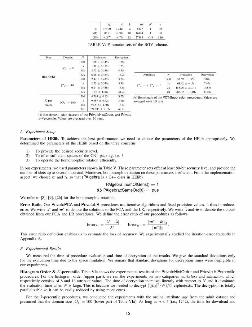
tk ` L m K κ
(I) 67499 1742 5 5227 1 90
(II) 8191 4096 10 16384 1 80
(III) ≈ 236 ≈ 70 32 27893 ≤ 8 110
TABLE V: Parameter sets of the BGV scheme.
Type Domain N Evaluation Decryption
Hist. Order
|Cj | = 8
500 1.26 ± 0.145s 1.26s1k 1.31 ± 0.157s 1.23s10k 2.72 ± 0.289s 4.80s32k 6.28 ± 0.484s 13.2s
|Cj | = 16
500 2.42 ± 0.439s 3.27s1k 2.53 ± 0.336s 3.30s10k 6.24 ± 0.448s 13.6s32k 13.8 ± 1.38s 41.2s
|Oj | = 100
500 4.768 ± 0.12s 3.27sK-per- 1k 9.487 ± 0.92s 3.11scentile 10k 97.515± 1.60s 18.6s
32k 321.285 ± 21.7s 48.8s
(a) Benchmark (adult dataset) of the PrivateHistOrder, and Privatek-Percentile. Values are averaged over 10 runs.
Attributes N Evaluation Decryption
|Cp| = 8, |Cq| = 6
500 35.69 ± 1.55s 3.84s1k 68.42 ± 4.17s 7.45s2k 155.26 ± 20.01s 14.83s4K 287.02 ± 10.10s 30.00s
(b) Benchmark of the PCT-Suppresion procedures. Values areaveraged over 10 runs.
A. Experiment Setup
Parameters of HElib. To achieve the best performance, we need to choose the parameters of the HElib appropriately. Wedetermined the parameters of the HElib based on the three concerns.
1) To provide the desired security level.2) To offer sufficient spaces of the CRT packing, i.e. `.3) To operate the homomorphic rotation efficiently.
In our experiments, we used parameters shown in Table V. These parameter sets offer at least 80-bit security level and provide thenumber of slots up to several thousand. Moreover, homomorphic rotation on these parameters is efficient. From the implementationaspect, we choose m and tk so that (PAlgebra is a C++ class in HElib)
PAlgebra::numOfGens() == 1&& PAlgebra::SameOrd(0) == true
We refer to [8], [9], [26] for the homomorphic rotation.
Error Ratio. Our PrivatePCA and PrivateLR procedures use iterative algorithms and fixed-precision values. It thus introduceserror. We write λ∗ and w∗ to denote the solutions to the PCA and the LR, respectively. We write λ and w to denote the outputsobtained from our PCA and LR procedures. We define the error ratio of our procedures as follows.
Errorλ∗ =|λ∗ − λ|λ∗
Errorw∗ =‖w∗ − w‖2‖w∗‖2
.
This error ratio definition enables us to estimate the loss of accuracy. We experimentally studied the iteration-error tradeoffs inAppendix A.
B. Experimental Results
We measured the time of procedure evaluation and time of decryption of the results. We give the standard deviations onlyfor the evaluation time due to the space limitation. We remark that standard deviations for decryption times were negligible inour experiments.
Histogram Order & K-percentile. Table VIa shows the experimental results of the PrivateHistOrder and Priavte k-Percentileprocedures. For the histogram order (upper part), we ran the experiments on two categories workclass and education, whichrespectively consists of 8 and 16 attribute values. The time of decryption increases linearly with respect to N and it dominatesthe evaluation time when N is large. This is because we needed to decrypt d(|Cj |2 ·N)/`e ciphertexts. The decryption is totallyparallelizable so it can be easily reduced by using more cores.
For the k-percentile procedures, we conducted the experiments with the ordinal attribute age from the adult dataset andpresumed that the domain size |Oj | = 100 (lower part of Table VIa). As long as n < ` (i.e., 1742), the time for download and
16
M T K Evaluation Decryption3 2 67.3 ± 4.89s 0.876s
10 4 3 99.9 ± 4.77s 0.848s5 3 122 ± 2.63s 0.874s3 3 70.6 ± 4.19s 0.848s
100 4 4 104 ± 7.68s 1.27s5 4 128 ± 7.93 1.26s3 3 72.7 ± 2.12s 0.96s
1000 4 4 108 ± 4.06s 1.25s5 5 136 ± 5.67s 1.43s
(a) PCA (for the first principal component)
M T K Evaluation Decryption1 1 173 ± 9.12s 0.475s
10 2 3 341 ± 8.12s 0.428s3 5 672 ± 9.76s 0.618s1 2 160 ± 3.97s 0.397s
100 2 4 400 ± 27.8s 0.649s3 7 787 ± 10.5s 0.816s1 2 164 ± 8.25s 0.388s
1000 2 4 383 ± 10.0s 0.622s3 8 865 ± 11.7s 0.944s
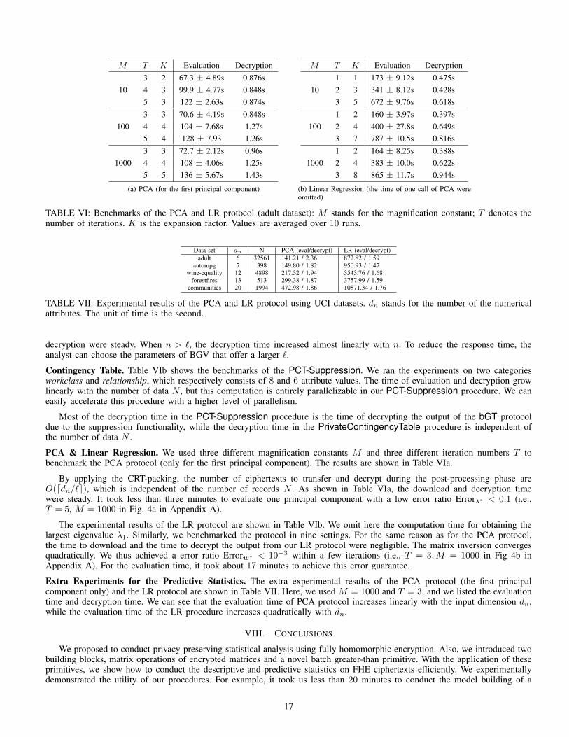
(b) Linear Regression (the time of one call of PCA wereomitted)
TABLE VI: Benchmarks of the PCA and LR protocol (adult dataset): M stands for the magnification constant; T denotes thenumber of iterations. K is the expansion factor. Values are averaged over 10 runs.
Data set dn N PCA (eval/decrypt) LR (eval/decrypt)adult 6 32561 141.21 / 2.36 872.82 / 1.59
autompg 7 398 149.80 / 1.82 950.93 / 1.47wine-equality 12 4898 217.32 / 1.94 3543.76 / 1.68
forestfires 13 513 299.38 / 1.87 3757.99 / 1.59communities 20 1994 472.98 / 1.86 10871.34 / 1.76
TABLE VII: Experimental results of the PCA and LR protocol using UCI datasets. dn stands for the number of the numericalattributes. The unit of time is the second.
decryption were steady. When n > `, the decryption time increased almost linearly with n. To reduce the response time, theanalyst can choose the parameters of BGV that offer a larger `.
Contingency Table. Table VIb shows the benchmarks of the PCT-Suppression. We ran the experiments on two categoriesworkclass and relationship, which respectively consists of 8 and 6 attribute values. The time of evaluation and decryption growlinearly with the number of data N , but this computation is entirely parallelizable in our PCT-Suppression procedure. We caneasily accelerate this procedure with a higher level of parallelism.
Most of the decryption time in the PCT-Suppression procedure is the time of decrypting the output of the bGT protocoldue to the suppression functionality, while the decryption time in the PrivateContingencyTable procedure is independent ofthe number of data N .
PCA & Linear Regression. We used three different magnification constants M and three different iteration numbers T tobenchmark the PCA protocol (only for the first principal component). The results are shown in Table VIa.
By applying the CRT-packing, the number of ciphertexts to transfer and decrypt during the post-processing phase areO(ddn/`e), which is independent of the number of records N . As shown in Table VIa, the download and decryption timewere steady. It took less than three minutes to evaluate one principal component with a low error ratio Errorλ∗ < 0.1 (i.e.,T = 5, M = 1000 in Fig. 4a in Appendix A).
The experimental results of the LR protocol are shown in Table VIb. We omit here the computation time for obtaining thelargest eigenvalue λ1. Similarly, we benchmarked the protocol in nine settings. For the same reason as for the PCA protocol,the time to download and the time to decrypt the output from our LR protocol were negligible. The matrix inversion convergesquadratically. We thus achieved a error ratio Errorw∗ < 10−3 within a few iterations (i.e., T = 3,M = 1000 in Fig 4b inAppendix A). For the evaluation time, it took about 17 minutes to achieve this error guarantee.
Extra Experiments for the Predictive Statistics. The extra experimental results of the PCA protocol (the first principalcomponent only) and the LR protocol are shown in Table VII. Here, we used M = 1000 and T = 3, and we listed the evaluationtime and decryption time. We can see that the evaluation time of PCA protocol increases linearly with the input dimension dn,while the evaluation time of the LR procedure increases quadratically with dn.
VIII. CONCLUSIONS
We proposed to conduct privacy-preserving statistical analysis using fully homomorphic encryption. Also, we introduced twobuilding blocks, matrix operations of encrypted matrices and a novel batch greater-than primitive. With the application of theseprimitives, we show how to conduct the descriptive and predictive statistics on FHE ciphertexts efficiently. We experimentallydemonstrated the utility of our procedures. For example, it took us less than 20 minutes to conduct the model building of a
17
linear regression on about 30k data of 6 features as input. We conclude that with applications of CRT-packing and appropriatedata encoding, securely conducting statistical analysis on large-scale datasets using a fully homomorphic encryption is becomingmore and more practical.
Acknowledgment. The authors would like to thank the useful and insightful comments from the reviewers and thank professorTakashi Nishide from University of Tsukuba for discussions on security analysis. This work is supported by JST CREST program“Advanced Core Technologies for Big Data Integration”. This work is further supported by the JSPS KAKENHI 24680015 and16H02864.
REFERENCES
[1] D. Boneh, C. Gentry, S. Halevi, F. Wang, and D. J. Wu, “Private database queries using somewhat homomorphic encryption,” in Applied Cryptographyand Network Security - 11th International Conference, ACNS 2013, Banff, AB, Canada, June 25-28, 2013. Proceedings, 2013, pp. 102–118.
[2] R. Bost, R. A. Popa, S. Tu, and S. Goldwasser, “Machine learning classification over encrypted data,” in 22nd Annual Network and Distributed SystemSecurity Symposium, NDSS 2015, San Diego, California, USA, February 8-11, 2015.
[3] Z. Brakerski, C. Gentry, and V. Vaikuntanathan, “(Leveled) fully homomorphic encryption without bootstrapping,” in Innovations in Theoretical ComputerScience 2012, Cambridge, MA, USA, January 8-10, 2012, 2012, pp. 309–325.
[4] Z. Brakerski and V. Vaikuntanathan, “Efficient fully homomorphic encryption from (standard) LWE,” in IEEE 52nd Annual Symposium on Foundationsof Computer Science, FOCS 2011, Palm Springs, CA, USA, October 22-25, 2011, 2011, pp. 97–106.
[5] ——, “Fully homomorphic encryption from ring-lwe and security for key dependent messages,” in Advances in Cryptology - CRYPTO 2011 - 31st AnnualCryptology Conference, Santa Barbara, CA, USA, August 14-18, 2011. Proceedings, 2011, pp. 505–524.
[6] J. Coron, A. Mandal, D. Naccache, and M. Tibouchi, “Fully homomorphic encryption over the integers with shorter public keys,” in Advances in Cryptology- CRYPTO 2011 - 31st Annual Cryptology Conference, Santa Barbara, CA, USA, August 14-18, 2011. Proceedings, 2011, pp. 487–504.
[7] C. Gentry, “A fully homomorphic encryption scheme,” Ph.D. dissertation, Stanford University (CA, USA), 2009.[8] C. Gentry, S. Halevi, and N. P. Smart, “Fully homomorphic encryption with polylog overhead,” in Advances in Cryptology - EUROCRYPT 2012 - 31st
Annual International Conference on the Theory and Applications of Cryptographic Techniques, Cambridge, UK, April 15-19, 2012. Proceedings, 2012,pp. 465–482.
[9] ——, “Homomorphic evaluation of the AES circuit,” in Advances in Cryptology - CRYPTO 2012 - 32nd Annual Cryptology Conference, Santa Barbara,CA, USA, August 19-23, 2012. Proceedings, 2012, pp. 850–867.
[10] O. Goldreich, Foundations of cryptography: volume 2, basic applications. Cambridge university press, 2009.[11] P. Golle, “A private stable matching algorithm,” in Financial Cryptography and Data Security, 10th International Conference, FC 2006, Anguilla, British
West Indies, February 27-March 2, 2006, Revised Selected Papers, 2006, pp. 65–80.[12] T. Graepel, K. E. Lauter, and M. Naehrig, “ML confidential: Machine learning on encrypted data,” in Information Security and Cryptology - ICISC 2012
- 15th International Conference, Seoul, Korea, November 28-30, 2012, Revised Selected Papers, 2012, pp. 1–21.[13] C. Guo and N. J. Higham, “A Schur-Newton method for the matrix pth root and its inverse,” SIAM J. Matrix Analysis Applications, vol. 28, no. 3, pp.
788–804, 2006.[14] S. Halevi and V. Shoup, “Algorithms in HElib,” in Advances in Cryptology - CRYPTO 2014 - 34th Annual Cryptology Conference, Santa Barbara, CA,
USA, August 17-21, 2014, Proceedings, Part I, 2014, pp. 554–571.[15] J. Hoffstein, J. Pipher, and J. H. Silverman, An introduction to mathematical cryptography. (Springer, New York), 2008.[16] N. Kirkendall and G. Sande, “Comparison of systems implementing automated cell suppression for economic statistics,” Journal of Official Statistics,
vol. 14, no. 4, p. 513, 1998.[17] V. Kolesnikov and T. Schneider, “Improved garbled circuit: Free XOR gates and applications,” in Automata, Languages and Programming, 35th International
Colloquium, ICALP 2008, Reykjavik, Iceland, July 7-11, 2008, Proceedings, Part II, 2008, pp. 486–498.[18] M. Lichman, “UCI machine learning repository,” 2013. [Online]. Available: http://archive.ics.uci.edu/ml[19] C. Liu, X. S. Wang, K. Nayak, Y. Huang, and E. Shi, “ObliVM: A programming framework for secure computation,” in 2015 IEEE Symposium on
Security and Privacy, SP 2015, San Jose, CA, USA, May 17-21, 2015, 2015, pp. 359–376.[20] W.-J. Lu, Y. Yamada, and J. Sakuma, “Privacy-preserving genome-wide association studies on cloud environment using fully homomorphic encryption,”
BMC medical informatics and decision making, vol. 15, no. Suppl 5, p. S1, 2015.[21] V. Lyubashevsky, C. Peikert, and O. Regev, “On ideal lattices and learning with errors over rings,” in Annual International Conference on the Theory and
Applications of Cryptographic Techniques. Springer, 2010, pp. 1–23.[22] R. Mises and H. Pollaczek-Geiringer, “Praktische verfahren der gleichungsauflosung.” ZAMM-Journal of Applied Mathematics and Mechanics/Zeitschrift
fur Angewandte Mathematik und Mechanik, vol. 9, no. 2, pp. 152–164, 1929.[23] S. U. Nabar and N. Mishra, “Releasing private contingency tables,” Journal of Privacy and Confidentiality, vol. 2, no. 1, p. 9, 2009.[24] M. Naehrig, K. E. Lauter, and V. Vaikuntanathan, “Can homomorphic encryption be practical?” in Proceedings of the 3rd ACM Cloud Computing Security
Workshop, CCSW 2011, Chicago, IL, USA, October 21, 2011, 2011, pp. 113–124.[25] M. Naor, B. Pinkas, and R. Sumner, “Privacy preserving auctions and mechanism design,” in Proceedings of the 1st ACM conference on Electronic
commerce, Denver, CO, USA. ACM, 1999, pp. 129–139.[26] V. S. Shai Halevi, “HELib,” http://shaih.github.io/HElib/index.html, accessed: 2014-12-10.[27] N. P. Smart and F. Vercauteren, “Fully homomorphic encryption with relatively small key and ciphertext sizes,” in Public Key Cryptography - PKC 2010,
13th International Conference on Practice and Theory in Public Key Cryptography, Paris, France, May 26-28, 2010. Proceedings, 2010, pp. 420–443.[28] ——, “Fully homomorphic SIMD operations,” Designs, codes and cryptography, vol. 71, no. 1, pp. 57–81, 2014.[29] D. Wu and J. Haven, “Using homomorphic encryption for large scale statistical analysis,” http://cs.stanford.edu/people/dwu4/FHE-SI Report.pdf, 2012.[30] A. C. Yao, “How to generate and exchange secrets (extended abstract),” in 27th Annual Symposium on Foundations of Computer Science, Toronto, Canada,
27-29 October 1986, 1986, pp. 162–167.[31] M. Yasuda, T. Shimoyama, J. Kogure, K. Yokoyama, and T. Koshiba, “Secure pattern matching using somewhat homomorphic encryption,” in Proceedings
of the 2013 ACM workshop on Cloud computing security workshop, Berlin, Germany. ACM, 2013, pp. 65–76.
18
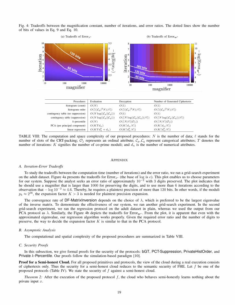
Fig. 4: Tradeoffs between the magnification constant, number of iterations, and error ratios. The dotted lines show the numberof bits of values in Eq. 9 and Eq. 10.
(a) Tradeoffs of Errorλ∗ (b) Tradeoffs of Errorw∗
Procedures Evaluation Decryption Number of Generated Ciphertexts
histogram (count) O(N) O(1) O(1)
histogram order O(d(|Cp|2N)/`e) O(d(|Cp|2N)/`e) O(d(|Cp|2N)/`e)contingency table (no suppression) O(N log(|Cp||Cq|)) O(1) O(1)
contingency table (suppression) O(N log(|Cp||Cq|)) O(dN log(|Cp||Cq|)/`e) O(dN log(|Cp||Cq|)/`e)k-percentile O(N) O(dN/`e|Oj |) O(dN/`e|Oj |)
PCA (per principal component) O(KTdn) O(Kddn/`e) O(Kddn/`e)linear regression O(KTd2n + dn) O(Kdd2n/`e) O(Kdd2n/`e)
TABLE VIII: The computation and space complexity of our proposed procedures: N is the number of data; ` stands for thenumber of slots of the CRT-packing; Oj represents an ordinal attribute; Cp, Cq represent categorical attributes; T denotes thenumber of iterations: K signifies the number of co-prime moduli; and dn is the number of numerical attributes.
APPENDIX
A. Iteration-Error Tradeoffs
To study the tradeoffs between the computation time (number of iterations) and the error ratio, we ran a grid-search experimenton the adult dataset. Figure 4a presents the tradeoffs for Errorλ∗ (the base of log is e). This plot enables us to choose parametersfor our system. Suppose the analyst seeks an error ratio of approximately 10−2 with 3 digits preserved. The plot indicates thathe should use a magnifier that is larger than 1000 for preserving the digits, and to use more than 6 iterations according to theobservation that − log 10−2 ≈ 4.6. Thereby, he requires a plaintext precision of more than 120 bits. In other words, if the modulipk ≈ 236, the expansion factor K > 3 is needed for plaintext precision expansion.
The convergence rate of DF-MatrixInversion depends on the choice of λ, which is preferred to be the largest eigenvalueof the inverse matrix. To demonstrate the effectiveness of our system, we ran another grid-search experiment. In the secondgrid-search experiment, we ran the regression protocol on the adult dataset in plain, whereas we used the output from ourPCA protocol as λ. Similarly, the Figure 4b depicts the tradeoffs for Errorw∗ . From the plot, it is apparent that even with theapproximated eigenvalue, our regression algorithm works properly. Given the required error ratio and the number of digits topreserve, the way to decide the expansion factor K is similar to that in the PCA protocol.
B. Asymptotic Analysis
The computational and spatial complexity of the proposed procedures are summarized in Table VIII.
C. Security Proofs
In this subsection, we give formal proofs for the security of the protocols: bGT, PCT-Suppression, PrivateHistOrder, andPrivate k-Percentile. Our proofs follow the simulation-based paradigm [10].
Proof for a Semi-honest Cloud. For all proposed primitives and protocols, the view of the cloud during a real execution consistsof ciphertexts only. Thus the security for a semi-honest cloud reduces to the semantic security of FHE. Let f be one of theproposed protocols (Table IV). We state the security of f against a semi-honest cloud.
Theorem 2: After the execution of the proposed protocol f , the cloud who behaves semi-honestly learns nothing about theprivate input x.
19
Proof: We can simply construct an ideal-world simulator Sfcloud for the view of the cloud in the real execution of f asfollows.
1. Sfcloud receives the encryption key pk and the specification about f , such as the number of inputs and the domain ofinputs (summarized in Table IV).
2. Sfcloud samples and computes Encpk(x) where x is chosen uniformly at randomly according to the specification of f .
3. Sfcloud outputs Encpk(x).
The view of the cloud in the real protocol execution is Vfcloud = {Encpk(x)} while the simulated view by Sfcloud is Vfcloud =
{Encpk(x)}. We immediately have Vfcloud ≈c Vfcloud from the the semantic security of the FHE.
Batch Greater-than. We prove that Algorithm 1 securely evaluates the greater-than functionality. Remind that Algorithm 1 isexecuted by the cloud. The decryptor receives JγK (Step 6) from the cloud and decrypts it to learn the greater-than result. Forsimplicity, we here prove for the case θ = 1. The proof can be readily generalized to the case of θ > 1 without loss of generality.
Theorem 3: For inputs a and b ∈ [D] (i.e., θ = 1), Algorithm 1 securely evaluates 1{a > b}. The decryptor learns 1{a > b}as the output of Algorithm 1 and nothing else.
Proof: We construct a simulator SbGT for the view of the decryptor in the real execution as follows.
1. SbGT receives the encryption key pk, the domain size D, and the evaluation result 1{a > b} as input.
2. SbGT samples a vector γ uniformly at random from (Zt/{0})D.
3. If 1{a > b} holds, SbGT chooses k∗ uniformly at random from [D] and sets γk∗ = 0.
3. SbGT outputs Encpk(Pack(γ)).
The simulated view for the decryptor is VbGT = {γ}. From the construction of Algorithm 1, the view of the decryptor in thereal execution is VbGT = {γ}. To prove the security of Algorithm 1, we need to show that VbGT and VbGT are indistinguishable.
We first show the distribution of γ in the real execution. According to Line 4 and Line 5 of Algorithm 1, we have
γk = (a− b− π0(k)) · rk for all k ∈ [D],
where π0 is a private random permutation π0 : [D]→ [D] generated by the cloud and rk is selected uniformly at random fromZt/{0}. In the case of a ≤ b, we have a − b − π0(k) 6= 0 for all k ∈ [D]. The value of γk, is thus, uniformly distributedin Zt/{0} due to the random value rk. On the other hand (i.e., a > b), we have one and only one k∗ ∈ [D] such thatγk∗ = a − b − π0(k∗) = 0. Furthermore, the value of k∗ distributes uniformly in [D] due to the random permutation π0. Thevalue of γk for all k 6= k∗ distributes uniformly on Zt/{0}. This is precisely the same distribution from which SbGT samplesthe γ, and we conclude that VbGT ≈c VbGT.
PCT-Suppression. We show the security of the PCT-Suppression protocol.
Theorem 4: The PCT-Suppression protocol securely computes Eq. 6. At the end of the execution of PCT-Suppression,the decryptor learns µ and nothing else.
Proof: Due to the independent random permutations πjs of bGT and the independent random values δ and r∗ of PCT-Suppression, the computation of
µs = µs · 1{µs > T }
is processed independently for each 1 ≤ s ≤ Σ. Thus, it suffices to show the security for a specific index s. We construct asimulator SPCT for the view of the decryptor in the real execution as follows (only for a specified index s).
1. SPCT receives the encryption key pk, and the evaluation result µs as input.
2. SPCT chooses γ′s and γ∗s uniformly at random from (Zt/{0})Σ.
3 SPCT chooses δs uniformly at random from Zt and sets µ′s = µs + δs.
4. If µs > 0 holds (i.e., no suppression), SPCT4.1 chooses k∗ uniformly at random from [Σ],4.2 sets the k∗-th element of γ′s as γ′
sk∗= δs,
4.3 sets the k∗-th element of γ∗s as γ∗sk∗
= 0.
5. SPCT outputs three ciphertexts: Encpk(µ′s), Encpk(Pack(γ′s)), and Encpk(Pack(γ∗s)).
The simulated view is VPCT = {µ′s, γ′s, γ∗s}. According to the construction of PCT-Suppression, the view of the decryptor in
the real execution consists of three components: VPCT = {µ′s,γ′s,γ∗s}. More specifically, µ′s = µs + δs (Step 5), γ′s = γs + δs
20

(Step 6) and γ∗s = γs × r∗s (Step 7). Recall that × is the element-wise multiplication and γs is the output (after decryption)of bGT(JµsK, JT K). Also, δs and r∗s are chosen uniformly at random from Zt and (Zt/{0})N , respectively. We need to showthat VPCT and VPCT are indistinguishable.
We first discuss the distribution of VPCT when µs ≤ T . In this case, from the proof of Theorem 3, the output of bGT(JµsK, JT K)consists of uniform random values from Zt/{0}. Thereby, elements of γ′s and γ∗s are also distributed uniformly on Zt/{0}.
When µs > T , there exists one and only one k∗ ∈ [Σ] such that γsk∗ = 0. Consequently, the k∗-th element of γ′s equals toδs and γ∗sk∗ = 0. The remaining elements of γ′s and γ∗s still distribute uniformly on Zt/{0}.
Moreover, in both cases, the value of µ′s distributes uniformly on Zt. This is precisely the same distributions from whichSPCT generates the µ′s, γ
′s, and γ∗s . We conclude that VPCT ≈c VPCT.
Histogram Order. We show the security of the PrivateHistOrder protocol. To show the proof, we firstly define an indexingfunction π : Cj → [|Cj |] such that kπ(sjp) = p for all 1 ≤ p ≤ |Cj |. For instance, when k = [2, 3, 1], this indicates that the indexesof attributes in the histogram sorted by the counts in ascending order is sj2, s
j3 and sj1. The indexing function π tells the index
of a specific state sjp in k, e.g., π(sj2) = 1.
Theorem 5: The PrivateHistOrder protocol securely evaluates Eq. 4. At the end of the execution of PrivateHistOrder, thedecryptor learns k and nothing else.
Proof: We leverage SbGT to construct a simulator SHistOrder for the view of the decryptor in the real execution ofPrivateHistOrder.
1. SHistOrder receives the encryption key pk, the number of data N , the domain size |Cj |, and the evaluation result k asinput.
2. For all (u, v) pairs where 1 ≤ u < v ≤ |Cj |, SHistOrder runs SbGT with inputs of pk, N , and 1{π(sju) > π(sjv)} (i.e.,θ = 1). For each invocation, we denote the output from SbGT as JγuvK.
3. SHistOrder outputs the ciphertexts {JγuvK}1≤u<v≤|Cj |.
The view of the decryptor in the real execution of PrivateHistOrder consists of outputs from independent invocations of bGT.Thereby, this is straightforward to see that the security of the PrivateHistOrder protocol is reduced to the security of bGTwhich has been shown in Theorem 3.
K-Percentile. We show the security of the Private k-Percentile protocol.
Theorem 6: The Private k-Percentile protocol securely computes Eq. 7. At the end of the execution of Private k-Percentile,the decryptor learns sjk∗ and nothing else.
Proof: We also leverage SbGT to construct a simulator Spercentile for the view of the decryptor in the real execution ofPrivate k-Percentile.
1. Spercentile receives the encryption key pk, the number of data N , the domain size |Oj | and the evaluation result sjk∗ asinput.
2. Spercentile generates a vector of boolean values f in which fp = 1{False} for all 1 ≤ p < k∗ and fp = 1{True} for allk∗ ≤ p ≤ |Oj |.
3. Spercentile runs SbGT with inputs of pk, N , and f (i.e. θ = |Oj |) and outputs the resulting ciphertexts from SbGT.
The view of the decryptor in the real execution of Private k-Percentile consists of the output from one invocation of bGT.Thereby, the security of the Private k-Percentile protocol also reduces to the security of bGT.
21