virtual dinosaurs developing computer aided design and ... · mallison, h.: virtual dinosaurs - cad...
TRANSCRIPT
Virtual Dinosaurs
- Developing Computer Aided Design and Computer Aided Engineering Modeling Methods for Vertebrate Paleontology
Dissertation zur Erlangung des Grades eines Doktors der Naturwissenschaften
der Geowissenschaftlichen Fakultät der Eberhard-Karls-Universität Tübingen
vorgelegt von
Heinrich Mallison aus Tübingen
2007

2
Tag der mündlichen Prüfung: 29. Mai 2007
Dekan: Prof. Dr. P. Grathwohl 1. Berichterstatter: Prof. Dr. W.-D. Reif 2. Berichterstatter: Prof. Dr. H.-U. Pfretzschner
Mallison, H.: Virtual Dinosaurs - CAD and CAE Modeling Methods for Vertebrate Paleontology
1
SUMMARY The use of personal computers offers many benefits to researchers compared to conventional methods, not the least of them the easy visualization of three-dimensional (3D) structures. With rapidly increasing computing power, the last few decades have seen the rise of a large number of new applications for many purposes, some of which have been successfully employed for vertebrate paleontology. Here, a description is given on how to use several commercially available computer aided design (CAD) and kinetic/dynamic Computer Aided Engineering (CAE) modeling software programs as tools for paleontological research. The focus rests on the creation and use of ‘virtual’ bones, for biomechanical analyses and use in reconstruction of entire skeletons, the use of these ‘virtual’ skeletons as tools for the creation of 3D ‘flesh’ models, which are helpful in mass estimates, and finally on multi-body kinetic/dynamic modeling, using these ‘flesh’ models to analyze posture and gait of extinct dinosaurs.
Specifically, the following techniques are described, most of which have been newly developed or significantly improved:
- Mechanical digitizing of fossil bones using Rhinoceros 3.0® and NURBS curves
- Mechanical digitizing of fossil bones using Rhinoceros 3.0® and point clouds
- Mounting ‘virtual’ skeletons from either mechanically digitized bones or CT-based data
- Creating 3D ‘flesh’ models from ‘virtual’ skeletons
- Creating 3D ‘flesh’ models from laser scan point cloud data of mounted skeletons
- Creating 3D ‘flesh’ models from silhouette drawings of skeletons
- Evaluating the accuracy of 2D and 3D reconstructions using ‘virtual’ skeletons
- Modeling posture, motions and locomotion of vertebrates in MSC.visualNastran 4D®.
CAD and kinetic/dynamic modeling using 3D CAE (Computer Aided Engineering) computer software prove to be useful tools for vertebrate paleontology, the latter being especially useful for biomechanical analysis.
These techniques were employed to study the prosauropod Plateosaurus engelhardti MEYER from the Löwenstein formation of South-West Germany. Aside from providing a new insight on mass estimates, it is shown that:
- Plateosaurus was not capable of pronating its manus sufficiently to use them in a support role during locomotion, nor can the animal have employed them in knuckle-walking with medially directed palms
- Plateosaurus was not well-balanced in a quadrupedal stance
- Plateosaurus was thus not capable of quadrupedal locomotion
- in addition, quadrupedal locomotion would be ineffective in Plateosaurus
- Plateosaurus was well-balanced when standing in a bipedal posture with a sub-horizontal backbone and tail
- Plateosaurus can execute all necessary motions, such as lying down and getting up from the ground from and into a bipedal stance, and can move the head to the ground without risking the stability of a bipedal stance.
A locomotion cycle for Plateosaurus was created in the kinetic/dynamic CAE software, showing bipedal locomotion to be feasible.
Mallison, H.: Virtual Dinosaurs - CAD and CAE Modeling Methods for Vertebrate Paleontology
2
Furthermore, it becomes apparent that
- there is a large amount of variation in the pes morphology of Plateosaurus engelhardti, requiring further study. Possibly, two or more species have been included in the taxon.
- Plateosaurus would likely have produced Otozoum-like tracks when walking bipedally, and Plateosaurus’ manus fits the manus imprints of Otozoum, made in a rare resting pose. The Otozoum-trackmaker was a biped.
- bipedal Pseudotetrasauropus tracks do not stem from animals with the pes morphology of the skeleton GPIT 1, but may have been produced by closely related animals.
Form these results it can be concluded that Plateosaurus was an obligate biped, and far closer to the basal mode of locomotion in sauropodomorphs than previously expected. It can be confidently refuted that plateosaurid dinosaurs created ichnofossils similar to Tetrasauropus.
Mallison, H.: Virtual Dinosaurs - CAD and CAE Modeling Methods for Vertebrate Paleontology
3
ZUSAMMENFASSUNG
Die Nutzung von PCs bietet Forschern viele Vorteile im Vergleich zu konventionellen Methoden, insbesondere die einfache Darstellung dreidimensionaler Strukturen. Mit der rasch wachsenden Rechenkapazität entstand in den letzten Jahrzehnten eine große Zahl von Anwendungen für eine Vielzahl von Bereichen, von denen einige erfolgreich in der Wirbeltierpaläontologie angewendet wurden. In dieser Arbeit wird beschrieben, wie verschiedene kommerziell erhältliche Computer Aided Design (CAD) und Computer Aided Engineering (CAE) Programme für kinetisch-dynamische Simulation in der paläontologischen Forschung verwendet werden können. Im Zentrum stehen die Erstellung und Nutzung von ‚virtuellen’ Knochen für biomechanische Analysen und zur Rekonstruktion ganzer Skelette, dann die Nutzung dieser ‚virtuellen’ Skelette als Handwerkszeug für die Erstellung von 3D Lebendmodellen, die zur Massenbestimmung nützlich sind, und schließlich die kinetisch-dynamische Vielkörper-Modellierung, in der die Lebendmodelle genutzt werden, um Körperhaltung und Gangarten von ausgestorbenen Dinosauriern zu untersuchen.
Die folgenden Methoden, von denen die meisten neu entwickelt oder stark verbessert wurden, werden beschrieben:
- Mechanisches Digitalisieren von fossilen Knochen in Rhinoceros 3.0® mittels NURBS (nicht-lienare rationale B-splines) Kurven
- Mechanisches Digitalisieren von fossilen Knochen in Rhinoceros 3.0® mittels Punktwolken
- Montage von ‚virtuellen’ Skeletten, sowohl aus mechanische digitalisierten Knochen als auch aus Daten aus der Computertomographie
- Erstellen von virtuellen 3D Lebendmodellen auf der Basis von ‚virtuellen’ Skeletten
- Erstellen von virtuellen 3D Lebendmodellen auf der Basis von Punktwolken-Laserscans montierter Skelette
- Erstellen von virtuellen 3D Lebendmodellen auf der Basis von Umrisszeichnungen von Skeletten
- Evaluierung der Genauigkeit von 2D und 3D Rekonstruktion mittels virtueller Skelette
- Modellierung von Körperhaltung, Bewegungen und Fortbewegung in MSC.visualNastran 4D®.
CAD und kinetisch-dynamische Modellierung mittels eines 3D CAE Programms stellen sich als nützliche Instrumente für die Wirbeltierpaläontologie heraus, wobei die Modellierung besonders für biomechanische Analysen hilfreich ist.
Diese Methoden wurden auf den Prosauropoden Plateosaurus engelhardti MEYER aus der Löwenstein-Formation Südwestdeutschlands angewandt. Neben neuen Erkenntnissen über Massenschätzungen wird gezeigt dass:
- Plateosaurus seine Hände nicht in einem Maße pronieren konnte, um sie während der Fortbewegung stützend einsetzen zu können, noch in der Lage war, sie mit einwärts zeigender Handfläche im Knöchelgang zu nutzen
- Plateosaurus in vierfüßiger Haltung nicht gut ausbalanciert war
- Plateosaurus daher nicht in der Lage war, sich vierbeinig fortzubewegen
- quadrupede Fortbewegung bei Plateosaurus außerdem ineffektiv wäre
- Plateosaurus in zweibeiniger Haltung mit annähernd horizontaler Wirbelsäule gut balanciert stand
Mallison, H.: Virtual Dinosaurs - CAD and CAE Modeling Methods for Vertebrate Paleontology
4
- Plateosaurus alle notwendigen Bewegungen wie Hinlegen und Aufstehen vom Boden aus und in eine bipede Haltung durchführen kann, und seinen Kopf auf Bodenniveau führen kann, ohne die Stabilität einer bipeden Haltung zu gefährden.
Im kinetisch-dynamischen CAE Programm wurde ein Gehzyklus für Plateosaurus erstellt, der zeigt, dass Plateosaurus zur bipeden Lokomotion fähig ist.
Außerdem zeigt sich, dass
- die Morphologie des Fußes von Plateosaurus eine große Varianz zeigt, die weitere Untersuchung erfordert. Möglicherweise sind zwei oder mehr Arten in dem Taxon zusammengefasst.
- Plateosaurus im bipeden Gang vermutlich Spuren hinterließ, die Otozoum ähneln und dass die Hand von Plateosaurus mit den Handabdrücken von Otozoum übereinstimmen, die der Verursacher nur selten beim Ruhen hinterließ. Der Verursacher der Otozoum-Spur war biped.
- bipede Spuren der Gattung Pseudotetrasauropus nicht von Tieren stammen, deren Fuß die gleiche Morphologie zeigt, wie das Skelett GPIT 1, möglicherweise aber von eng verwandten Tieren.
Aus diesen Resultaten lässt sich schließen, dass Plateosaurus obligat biped lief, und der basalen Fortbewegungsart der Sauropodomorpha weit näher blieb als bisher angenommen. Es kann außerdem mit hoher Sicherheit ausgeschlossen werden, dass Plateosaurus Spuren ähnlich dem Ichnotaxon Tetrasauropus hinterließ.
Mallison, H.: Virtual Dinosaurs - CAD and CAE Modeling Methods for Vertebrate Paleontology
5
TABLE OF CONTENT SUMMARY .................................................................................................................................1 Zusammenfassung...................................................................................................................3 TABLE OF CONTENT ...............................................................................................................5 GENERAL INTRODUCTION AND OVERVIEW OF THE PROJECT........................................7
GENERAL INTRODUCTION..................................................................................................7 Overview of the project ......................................................................................................7 Institutional abbreviations ..................................................................................................8 Computer softwares...........................................................................................................9 Technical equipment ..........................................................................................................9 Plateosaurus posture and locomotion - state of the art .....................................................9
SECTION I................................................................................................................................13 SUMMARY OF SECTION I ..................................................................................................13 INTRODUCTION TO SECTION I.........................................................................................13 AIMS.....................................................................................................................................15 MATERIAL AND METHODS................................................................................................15
Equipment and materials .................................................................................................15 Prerequisites ....................................................................................................................15 General Overview of the Digitizing Procedure.................................................................16
THE DIGITIZING TECHNIQUES IN DETAIL .......................................................................18 Setting things up ..............................................................................................................18 The techniques: Coordinate placement, recalibration and seam line placement ............19 The techniques: Gathering data - open and closed curves, point clouds........................20 The techniques: Editing data ...........................................................................................21 The techniques: Creating bodies - lofting and joining surfaces .......................................22
APPLICATIONS OF TECHNIQUES TO DIFFERENT SPECIMEN TYPES ........................22 Digitizing with closed curves – general remarks..............................................................22 Digitizing with closed curves – small bones (simple shapes) ..........................................22 Digitizing with closed curves – medium sized bones.......................................................23 Digitizing with closed curves – large bones .....................................................................23 Digitizing with composite closed curves (very large bones and/or complex bone shapes).........................................................................................................................................23 Digitizing bones as composite bodies with separate curve sets - complex bone shapes.........................................................................................................................................24 Digitizing with point clouds/meshes (small bones with complex shapes, partially inaccessible bones) .........................................................................................................25 Marking surface features .................................................................................................25 Composite bones from partially preserved specimens....................................................25
EXTRACTING VIRTUAL BONES FROM CT DATA ............................................................26 ACCURACY OF MECHANICAL DIGITIZING DATA ...........................................................26 DISCUSSION: BENEFITS AND LIMITATIONS OF DIGITIZED DATA ...............................28 CONCLUSIONS REGARDINGS THE METHODS ..............................................................29 APPLICATION IN THIS STUDY ..........................................................................................30
Digitized material of Plateosaurus ...................................................................................30 Other genera and objects ................................................................................................30
SECTION II ...............................................................................................................................31 INTRODUCTION TO SECTION II........................................................................................31 AIMS.....................................................................................................................................32 DIGITAL MODEL CREATION..............................................................................................33
Virtual bones and virtual skeletons ..................................................................................33 Virtual skeletons created in this study .............................................................................35 Virtual ‘life’ models ...........................................................................................................39 Virtual ‘life’ models created in this study..........................................................................42
COMPARING THE VIRTUAL SKELETON TO PREVIOUS RECONSTRUCTIONS...........45 COMPARING THE VIRTUAL SKELETON TO 3D MODELS ..............................................49 DISCUSSION .......................................................................................................................52
Skeletal reconstruction.....................................................................................................52 Soft tissue reconstruction and body mass .......................................................................53
CONCLUSIONS SECTION II ...............................................................................................54
Mallison, H.: Virtual Dinosaurs - CAD and CAE Modeling Methods for Vertebrate Paleontology
6
SECTION III ..............................................................................................................................56 INTRODUCTION TO SECTION III.......................................................................................56 AIMS.....................................................................................................................................58 BASICS OF LOCOMOTION RESEARCH ...........................................................................58 INTRODUCTION TO THE MODELING SOFTWARE..........................................................59
Model components and properties ..................................................................................60 Simulation results.............................................................................................................61 Model creation .................................................................................................................62
CREATING A VERTEBRATE MODEL IN MSC.visualNastran 4D® ...................................64 Creating and importing 3D bodies ...................................................................................65 Connecting bodies with constraints .................................................................................67
CONTROLING THE SIMULATION ......................................................................................72 Data input types ...............................................................................................................72 Creating a motion sequence ............................................................................................73
MEASURING A SIMULATION .............................................................................................75 APPLICATION IN THIS STUDY ..........................................................................................76
Static analyses - center of mass......................................................................................76 Dynamic analyses: Posture and Balance ........................................................................79 Dynamic analyses: motions of the neck and tail versus the body, range of motion ........88 Dynamic analyses: locomotion cycles .............................................................................92 Assessment of quadrupedal posture ...............................................................................96 Calibrating simulation results with external data..............................................................97 Future Research ..............................................................................................................98
CONCLUSIONS SECTION III ..............................................................................................99 IMPLICATIONS FOR THE AUTECOLOGY OF PLATEOSAURUS .......................................99 CONCLUSIONS .....................................................................................................................100 ACKNOWLEDGEMENTS ......................................................................................................102 Figures
For ease of use, all Figures can be found in black and white in a separate section at the back of this volume. Additionally, they can be found in color in the ‘Figures’ folder on the accompanying DVD, and in the ‘Figure.doc’ text file, which also includes the captions.
Video files
As most video files mentioned in the text show simulation results, they can be found in the ‘Simulation files’ folder of the accompanying DVD. Those that are not part of a simulation run can be found in the subfolder ‘other videos’.
Simulation data All references in the text to simulation data refer to the MSC.visualNastran 4D® files, which carry the file extension *.WM3. As these can only be viewed with MSC.visualNastran 4D® and similar programs, simulation results were exported in the form of Windows® videos (file extension *.avi) and Simulation reports in HTML format, which can be displayed on any standard PC with Microsoft Windows® installed. Graphs referred to in the text are not provided as separate image files, but are included in the Simulation report. All this data can be found in the ‘Simulations’ folder on the accompanying DVD. At the beginning of the description of a simulation file, the name of the *.WM3 file is given; thereafter, no repetitive reference is made to the file or graphs, as they can be found through the simulation file name. All videos and simulation reports carry the same name as the simulation file they derive from. Some videos have additions to their name, which indicates what type of data they contain in addition to the main simulation display. For example, ‘S007-A orient hip meter.avi’ is the video file of simulation run S007-A.wm3, with the data of a meter on the hip joint displaying hip orientation superimposed.
Appendices Appendix A - Guide to digitizing and model creation techniques for Rhinoceros 3.0®
Appendix B - Guide to point cloud and polygon mesh editing in Geomagic Qualify®
Appendix C - Files on DVD
Mallison, H.: Virtual Dinosaurs - CAD and CAE Modeling Methods for Vertebrate Paleontology
7
GENERAL INTRODUCTION AND OVERVIEW OF THE PROJECT
GENERAL INTRODUCTION
Overview of the project The scientific investigation undertaken in the project presented here developed out of a long-standing interest in dinosaur locomotion. The Research Unit FOR 533 ‘Biology of the Sauropod Dinosaurs - the Evolution of Gigantism’ studies the factors that allowed gigantism to develop in sauropods. This project, ‘Plateosaurus in motion’ (C6) of the FOR 533, was intended to investigate the possibilities of applying new and more powerful computer tools such as computer aided design (CAD) and kinetic modeling to vertebrate paleontology, using the example of Plateosaurus engelhardti MEYER (Meyer 1837). The Institute for Geosciences (IFGT) of the Eberhard-Karls-Universität in Tübingen, Germany, houses two complete skeletal mounts and additional skeletal material of Plateosaurus, the best known early sauropodomorph dinosaur, and the Staatliches Museum für Naturkunde, Stuttgart, housing several more excellent specimens, is within easy reach. This provided an ideal opportunity to study the biomechanics of this well-known but highly controversial genus.
One task in this project was to provide other projects of the research unit with more accurate mass and surface area data on Plateosaurus and other relevant dinosaurs.
Through kinetic computer modeling the biomechanical adaptations on the way from obligate bipedality via facultative quadrupedality to fully obligate quadrupedality had to be investigated.
During the course of the project it became apparent that mass estimates with the planned mathematical method would be easily possible, but also that other methods, based on computer aided design (CAD) offered the additional advantages of easier visualization and potentially more accurate mass estimates, allowed more flexibility and provided the required digital 3D files for kinetic modeling at the same time. Therefore, the focus of this project shifted slightly, emphasizing as the first goal the acquisition and processing of data by development of new and improved techniques. Additionally, early results indicated that Plateosaurus was an obligate biped, stressing the need to investigate the range of motion of the limb joints and the exact position of the center of gravity even more detailed than planned before. In addition to an analysis of the walking cycle in a commercially available rigid body modeling software, MSC.visualNastran 4D®, the questions of balance and torques required for a bipedal posture became the main aims of the modeling phase. Therefore the project has three parts, each split into the two aspects of development of methods and application of them to Plateosaurus.
The first part deals with new and improved methods for data acquisitions with a mechanic digitizer and details the extraction of data from computer tomography scans, both in order to create ‘virtual bones’. These methods are compared with regards to their accuracy.
The second part describes methods for creating ‘virtual skeletons’ and ‘virtual life models’ from these and other data sources. The methods are compared for accuracy by applying them not only to Plateosaurus, but also to a Recent species, Elephas maximus. The giant sauropod Brachiosaurus brancai is also modeled, in part to prepare later modeling of that famous animal in MSC.visualNastran 4D®, but especially as a means of comparing the methods developed here to those employed by the research group of H.-C. Gunga [Project B2 ‘Metabolism’ of FOR 533] (e.g. Bellmann et al. 2005, Gunga et al. 1999, Gunga et al. 1995, Gunga et al. in press, Suthau et al. 2005). Additionally, various published reconstruction drawings are compared to the new data and their reliability evaluated. The use of ‘virtual bones’ and ‘virtual skeletons’ also allows assessments of the ranges of motion of
Mallison, H.: Virtual Dinosaurs - CAD and CAE Modeling Methods for Vertebrate Paleontology
8
joints; here, properly articulating humerus, radius and ulna and the determination of the amount of manus pronation possible were important.
The third part outlines the modeling of Plateosaurus in MSC.visualNastran 4D® and describes comparison of the results to ichnofossils. Also, implications for the evolutionary history of quadrupedality in sauropodomorphs are discussed.
The methods developed in this project are based on each other: exact 3D skeletal models allow reconstructing soft tissue masses and their distributions more exactly than previous methods, and three-dimensional models can be created far more easily and with higher accuracy. These in turn, together with the better known weights, allow far more complex and accurate kinetic/dynamic simulations, while previous approaches were often limited to extremely simplified kinematical modeling. The novelty of the methods developed for this project lies in the ability to increase accuracy, reduce work time and address more complex problems than conventional methods allow, which makes future analyses comparing many taxa or groups more feasible.
Due to the three part nature of the work, this thesis is somewhat unusual in the arrangement of its content. Instead of the usual ‘material and methods’ chapter, only a list of the institutions and the computer programs used is given, along with an overview of the state of the art of the research on Plateosaurus. Then, three sections detail the work on the three aspects of digitizing techniques (SECTION I), 3D skeletal and flesh model creation and mass estimates as well as comparison to older reconstructions (SECTION II) and kinetic modeling in MSC.visualNastran 4D® (SECTION III). In each section, material and methods are described in detail and the results given, along with a short discussion of their relevance within the specific context of that project part. Then, two chapters contain the discussion of the results in the general context of the project, the first with regards to the methodology and the second with regards to Plateosaurus and the evolution of sauropodomorph locomotory patterns. Finally, the appendices contain detailed ‘how to’ instructions for the use of the employed softwares Rhinoceros 3.0®, Geomagic Qualify 8.0® in order to facilitate the application of the techniques by other researchers. The use of MSC.visualNastran 4D® is described in detail in SECTION III, as a detailed understanding of the program is required to grasp the modeling described in that part of the thesis.
Institutional abbreviations AMNH American Museum of Natural History, New York (US)
BSP Bayrische Staatssammlung für Paläontologie und Geologie, München (GER) (formerly Bayrische Staatssammlung für Paläontologie und historische Geologie)
IFGT Institut für Geowissenschaften, Eberhard-Karls-Universität Tübingen (GER) (formerly GPIT: Geologisch-Paläontologisches Institut)
GPIT see IFG
HMNB Museum für Naturkunde der Humboldt-Universität Berlin (GER)
(also abbreviated MN or HMN in literature)
JRDI Judith River Dinosaur Institute, MT (USA)
MHH Museum Heineanum, Halberstadt (GER)
MSF Museum Saurierkommission Frick, Tonwerke Keller A.G., Frick,
Kanton Aargau (CH)

Mallison, H.: Virtual Dinosaurs - CAD and CAE Modeling Methods for Vertebrate Paleontology
9
PMG Paleon Museum, Glenrock, WY (USA)
SMA Sauriermuseum Aathal, Aathal-Seegräben (CH)
SMNS Staatliches Museum für Naturkunde Stuttgart (GER)
ZMK Zoological Museum, University of Kopenhagen (DK)
ZST Zoological Display Collection, Eberhard-Karls-Universität Tübingen (GER)
Computer softwares The following three programs are indispensable for the techniques described here:
(1) McNeel Associates ‘Rhinoceros© 3.0 NURBS modeling for Windows®’
Rhinoceros 3.0® is a NURBS based CAD program.
(2) MSC Corporation™ ‘MSC.visualNastran 4D®’
MSC.visualNastran 4D® is a rigid body modeling software for FEA (finite element analysis) and kinetic/dynamic modeling.
(3) TGS Template Graphics Software Inc. ‘AMIRA 3.11’ (time-limited evaluation version)
AMIRA 3.11 is a 3D visualizing and modeling system that allows creation of surfaces (3D bodies) from computer tomography (CT) data.
Other software used in this project:
(4) Geomagic Corporation ‘Geomagic Qualify 8.0®’ (time-limited evaluation version)
Geomagic Qualify 8.0® is a CAQ (computer aided quality assurance) program.
Technical equipment Immersion™ ‘Microscribe 3D’ mechanical digitizer
Immersion™ ‘Microscribe 3GL’ mechanical digitizer (on loan from the Institut für Zoologie der Rheinischen Friedrich-Wilhelm-Universität Bonn)
The GL version of the digitizer has a longer arm, allowing for a greater reach with only a negligible loss in accuracy.
Plateosaurus posture and locomotion - state of the art
The skeletal material of Plateosaurus on exhibit at the Institute for Geosciences in Tübingen stems from the excavation at Trossingen in the Black Forest of SW Germany led by the famous Friedrich von Huene, who had one nearly complete individual (GPIT skeleton 1, often
Mallison, H.: Virtual Dinosaurs - CAD and CAE Modeling Methods for Vertebrate Paleontology
10
simply referred to as GPIT1) mounted in a bipedally standing pose (Figure 1), head close to the ground as if drinking or eating (Huene 1926). A second mount (GPIT2), the animal apparently running at high speed with the torso raised steeply to an angle of over 45°, consists of two parts: from the atlas to the third to last presacral, the bones belong to one individual, the third to last presacral itself is missing and replaced by a plaster model, and the hind part of the mount belongs to another individual. This mount has a better preserved sinistral manus and sinistral pes than GPIT1. On both mounts, the dextral manus and pes are less well preserved than the contralateral side, and lack more elements.
Since Plateosaurus is a relatively basal sauropodomorph that was discovered quite early and is known from much more material than many other Triassic dinosaurs, the finds have caused heated debate about the locomotory adaptations of the animal. Huene (1907-1908) argued for digitigrade bipedality and attributed a grasping function to the manus. He was convinced that Plateosaurus was an obligate biped, much as the similar Anchisaurus that had been described as bipedal and digitigrade by Marsh (1893a, 1893b). A good indicator for this is the highly divergent length of fore- and hindlimbs. Despite later criticism from many sources, von Huene adamantly stuck to this interpretation of the material, and had the mounts of GPIT1 and GPIT2 set up in Tübingen in bipedal postures.
Later researchers have suggested practically any possible stance: obligate quadrupedality and plantigrady ‘like lizards’ was proposed by Jaekel (1910), who later revised himself and concluded a clumsy, kangaroo-like hopping as the only possible mode of locomotion (Jaekel 1911). Fraas referred to the position of the skeletal finds in the field, arguing for a sprawling gait (Fraas 1912, 1913). He had the skeleton SMNS 13200 mounted in this position in the Stuttgart museum.
Later, researchers began to agree with Huene on the issue of digitigrady, although plantigrady makes a comeback in Sullivan et al. (2003): Weishampel and Westphal (1986) depict Plateosaurus running digitigrade and bipedally, but they argue for facultative quadrupedality. Interestingly, the metacarpals are depicted widely spread, in marked contrast to the interpretation by Huene (1926), but see reconstruction drawing in that publication, as discussed below), a position that does not seem to fit an active role of the manus in locomotion. Paul (1997) also argues for bipedality, but his outlined skeletal drawing seems to imply permanent rather than facultative quadrupedality. Another proponent of bipedality is Van Heerden (1997).
Among others, Galton (1971, 1976, 1990) advocates quadrupedality in prosauropods. He based his opinion on the hindlimb to trunk and hindlimb to forelimb ratios, the latter also being invoked by Bonaparte (1971). Wellnhofer (1994) also depicts Plateosaurus in a quadrupedal stance, based on characteristics of the tail of material from Ellingen (Bavaria) now in the BSP, which he figured with a strong downward curve making a bipedal stance impossible.
In the first functional morphology approach on Plateosaurus locomotion, Christian et al. (1996) studied the vertebral column’s resistance to bending in various vertebrates in order to determine their locomotory modes. Since Plateosaurus shows an intermediate pattern between obligate bipeds and obligate quadrupeds, exhibiting a medium peak of resistance to bending over the shoulders instead of either the small peak of bipeds or the large peak of quadrupeds, Christian et al. (1996) argue that the animal was probably facultatively bipedal at high speeds only. They also investigated the shape of the acetabulum and agree with Huene (1926) on a near-vertical position of the femur instead of a more sprawled configuration.
The latest extensive publication on the osteology of Plateosaurus (Moser 2003) claims that Plateosaurus would only have been capable of tiny shuffling steps when walking bipedally. He describes also the remounting of the skeletal mount previously exhibited in the Bayrische Staatssammlung in Munich for the Naturhistorische Gesellschaft in Nuremberg. The animal was forced into what (Moser (2003) calls the track of a quadrupedal prosauropod (probably the track depicted in Moser 2003: fig. 28, Tetrasauropus unguiferus, from Ellenberger [1972]), despite the fact that the track exhibits inwardly curved toes and fingers while all articulated finds of Plateosaurus and the morphology of the phalangal articular surfaces indicate no lateral bending of the toes or fingers. Moser (2003) suggests that this discrepancy may indicate an early sauropod instead of a prosauropod as the trackmaker. The ichnofossil Otozoum, originally described by Hitchcock (1847) and redescribed by Rainforth (2003), is another candidate for a prosauropod track: a bipedal track with two manus imprints on which
Mallison, H.: Virtual Dinosaurs - CAD and CAE Modeling Methods for Vertebrate Paleontology
11
the fingers point outward at a right angle to the direction of movement. The imprints fit the shape of the Plateosaurus manus and pes. The pes of Plateosaurus has been claimed also to fit the pes print of Pseudotetrasauropus, suggested as another possible prosauropod track by Lockley and Meyer (2000); Porchetti and Nicosia (2007) also conclude that Plateosaurus is a possible creator of this ichnofossil. Nicosia and Loi (2003) describe a new ichnotaxon, Evazoum siriguii. They claim that the foot of Sellosaurus as depicted in Galton (1990) best fits the track, although there is a distinct size difference. From this they conclude that a small prosauropod with fan shaped feet with splayed digits created these tracks. Potentially, juvenile of Plateosaurus could be considered to have created them.
Overlapping with the project presented here, Bonnan and Senter (2007) investigate the elbow joints of Plateosaurus, the closely related prosauropod Massospondylus and their extant phylogenetic bracket (Alligator, Anser and Struthio being the examples of choice) with regards to their mobility. In marked contrast to most previous researchers, they find that Plateosaurus could neither pronate the hand, nor did the animal show any adaptations to knuckle-walking with medially facing palmar surfaces of the hand. Therefore, they argue for obligate bipedality again, as Huene already did almost exactly a hundred years before (Huene 1907-1908). Bonnan and Yates (2007) also redescribed the forelimb of Melanorosaurus, a basal sauropod that is superficially similar to Plateosaurus in morphology, but for several important adaptations that make it an obvious obligate quadruped. This animal may be the real Tetrasauropus trackmaker.
Another hotly debated issue was the articulation of the pectoral girdle in Plateosaurus. As with most dinosaurs, no consensus seemed to exist regarding the mobility of the scapulacoracoids and their position on the ribcage. Paul (1987) arranges the putative clavicles in a manner that leaves the shoulder girdle highly mobile, but this interpretation was challenged by Yates and Vasconcelos (2003), who described an articulated pair of clavicles in Massospondylus, interpret it as a furcula-like bracing structure. Recent dinosaur finds have brought to light a plethora of claviculae and furculae even in groups widely removed from the developed theropods who gave rise to modern birds, with the most impressive example the boomerang shaped furcula of the diplodocid sauropod baby ‘Tony’ (see Figure 2 and Ikejiri et al. [2005]). In adult derived sauropodomorphs, scalupar rotation also appears to be absent (Henderson 2007). Hence, a similar arrangement in Plateosaurus is likely, negating motion within the pectoral girdle. The scapula has been placed in a variety of angles to the vertebral column. Recent research, e.g. by Schwarz et al. (2006), seems to indicate that an angle between 55° and 60° from the horizontal is the plesiomorphic condition in dinosaurs.
The taxonomy of Plateosaurus is beyond the scope of this paper. Moser (2003) gives an extensive review of its complicated and confusing history and makes a strong case for a monospecific genus. GPIT1 and GPIT2 are therefore here referred to as Plateosaurus engelhardti, although they are listed as P. longiceps in Galton and Upchurch (2004).Yates (2003) agrees with Moser (2003), and places material formerly referred to Sellosaurus into a second species of Plateosaurus, P. gracilis. For the purpose of this study, it is irrelevant whether the different individuals from the Halberstadt, Trossingen, Ellingen (all Germany) and Frick (Switzerland) localities belong to one or several closely related species or genera, since their differences that might influence locomotion are minimal. The sister taxon Massospondylus is sufficiently similar so that biomechanical conclusions can be expanded to it from Plateosaurus. Massospondylus hatchlings have been described as quadrupedal (Reisz et al. 2005), and the ontogenetic shift to bipedality is of great interest, since it may shed light on the evolution of sauropod locomotion.
Since much of the work here uses the GPIT1 skeleton extensively, and is partly based on a laser scan of the mounted skeleton, a short description of the fossil material and its mount is appropriate. The fossils represent one nearly complete individual of Plateosaurus engelhardti. Without thin sectioning the bone it is hard to judge the ontogenetic stage of the animal. Sander and Klein (2005) have found a previously unexpected amount of plasticity in the growth of Plateosaurus, so size is not a good proxy for age in these animals. Additionally, many size estimates for Plateosaurus in the literature are overestimation, based on massively
Mallison, H.: Virtual Dinosaurs - CAD and CAE Modeling Methods for Vertebrate Paleontology
12
deformed bones (Moser 2003). A better indicator would be the amount of fusion of skull bones, but the cranium is missing. Hence, it can only be deduced that the animal is too large to be a juvenile. The skeleton was discovered semi-articulated and lacks the skull and mandibles and some parts of the hands and feet. A few appendicular elements are deformed, albeit most only slightly (e.g. left tibia, left coracoid). Most of the dorsal and caudal vertebrae are slightly distorted, the transverse processes of the left side tilting downward and those of the right side tilting upward, each by roughly 20°. The first sacral vertebra exhibits a more distinct deformation, the cranial surfaces being tilted backwards quite considerably. The ribs were fractured into small pieces and their current shapes do not relate to their shapes in life. The mount (Figure 1) articulates almost all non-deformed bones well, and takes the almost symmetrical deformation of the vertebrae into account. Thus, the ribs are positioned averaging the position of the articulation surfaces on the right and left side. Sacral 1 is disarticulated from the last presacral, and placed rather in a straight continuation of the vertebral column assuming the original proportions of sacral 1 to be similar to sacral 2, with parallel anterior and posterior faces. The only instance in which the mount is problematic in a significant way is the distal splaying of the metacarpals, which enlarges the palm of the hand to an unreasonable extent. Were they to be shown correctly, the metacarpals should be arranged sub-parallel and in close contact with one another, with equal contact both proximally and distally.
Mallison, H.: Virtual Dinosaurs - CAD and CAE Modeling Methods for Vertebrate Paleontology
13
SECTION I
SUMMARY OF SECTION I
Three-dimensional digitized representations of large bony elements offer certain advantages over casts or real bones. However, creation of 3D computer files can be time consuming and expensive, and the resulting files difficult to handle. Hitherto, mechanical digitizing was also limited to large bones. In this section, new and improved data collection techniques for mechanical digitizers are described which facilitate file creation and editing. This includes:
- Specifics for an easy to assemble and transportable holder for small fossils.
- Improvements to the in-program digitizing procedure, removing the need for additional editing software and reducing time and financial demands.
- A significant increase in the size range of bones that can be digitized, allowing both exact digitizing of bones of only a few centimeters in size and bones larger than the range of the digitizer arm. This allows the study of structures that include both small and large bones.
- Complex shapes such as costae and vertebrae can now be digitized with ease.
- Step-by-step directions for digitizer and program use to facilitate easy acquisition of the techniques.
Fossils digitized with the methods described can easily be added to online databases, both as small-scale preview and as complete files. The acquired data serves as the basis for 3D model creation for the mass analysis and kinetic modeling conducted during this project. The file formats are common and the file sizes relatively small in comparison to CT or laser scan data. Pointcloud files can be used interchangeably with laser scan files of similar resolution. Other possible uses for data created with these methods are described.
Additionally, the techniques employed to extract and edit CT data for model creation are briefly described.
INTRODUCTION TO SECTION I
In recent year, digital files have increasingly been used for scientific research instead of real bones or casts. Currently, the most common way of obtaining a digital representation of a specimen is computer assisted tomography (CT) (see e.g. Golder and Christian 2002, Gould et al. 1996, Knoll et al. 1999, Ridgely and Witmer 2004, 2006, Stokstad 2000, Zuo and Jing 1995). These digital images can consist of cross sections, but usually are three dimensional models of internal shapes of an object, e.g. in order to assess as yet unprepared specimen or depict internal structures without damaging the object. Models of external shapes, on the other hand, are used to rapid prototype (RP) scaled models or exhibit copies, since the high accuracy of CT scans justifies the high costs of CT scanning and RP. This technique also allows mirroring of specimen or combining several partial specimens into one complete individual or bone. Recently, neutron tomography (NT) has also been tested (Schwarz et al. 2005) with mixed results.
Another method to obtain 3D files is laser scanning, either from three perpendicular views or with a surround scan. Alternatively, repeated scans can be taken at many angles and combined in the computer. Currently, an extensive project is underway at the Technische

Mallison, H.: Virtual Dinosaurs - CAD and CAE Modeling Methods for Vertebrate Paleontology
14
Universität Berlin using laser scanners to digitize complete mounted skeletons and skin mounts (http://www.fpk.tu-berlin.de/projekte/sonder/arbeit/dino/projekt.phtml, see also Bellmann et al. 2005, Gunga et al. 1999, Gunga et al. 1995, Gunga et al. in press, Suthau et al. 2005). This included a high resolution scan of GPIT 1 (Figure 3). Also, some of the dinosaur skeletons mounted in the MNHB exhibition were high resolution laser scanned by Research Casting International (www.rescast.ca) during the museum renovation in 2006/2007 as separate elements.
All three methods produce vast amounts of data, depicting the object in very high detail. When such high resolution is not needed the large file size becomes cumbersome. As long as only external surfaces are of concern, mechanical digitizing provides a cheap and fast alternative (Wilhite 2003a, 2003b), delivering small files of sufficient accuracy for most applications. Other techniques involving digitizing were used by Goswami (2004) and Bonnan (2004), who focused on bone landmarks, and will not be addressed here. Similar in handling and data output to the methods described here is the sonic digitizer used e.g. by Hutchinson et al. (2005). It is limited to collecting point data, but provides a large range of up to 14 feet.
This section details improvements for digitizing techniques for dinosaur bones described by Wilhite (2003b), expanding the size range of suitable bones for the method significantly. New methods allowing complex shapes to be digitized with relative ease are also described. Also, the extraction of surface data from CT data in AMIRA 3.11® and the subsequent editing is described briefly.
Fossils digitized with the methods described here can easily be added to online databases, instead of or alongside with photographic images. Most databases, such as the database of the New Mexico Museum of Natural History (Hester et al. 2004) or the American Museum of Natural History (http://research.amnh.org/amcc/database/), can easily accommodate small-scale previews as well as complete files, since the file formats are common and the file sizes relatively small in comparison to CT or laser scan data. Stevens (www.dinomorph.com) uses several files created during this project for modeling Brachiosaurus in Dinomorph™. The University of Texas runs another digital library (http://www.digimorph.org/index.phtml), based on High-Resolution CT scans. Objects digitized via dense point clouds as described herein could conceivably be added to this database as stereolithographies (*.stl files), provided sufficient resolution is obtained. For most applications, pointcloud files created with the Microscribe® can be used interchangeably with laser scan files of similar resolution. The digital files can also be used to easily test possible skeletal assemblages, joint mobility ranges (see Wilhite 2003a, b), and can be an aid in planning museum mounts.
Another possible application is rapid prototyping. Scale models of bones can be produced at almost any scale, as well as molds for casting, or negatives of the bones that can serve as storage casts or as mounting racks for museum exhibition. High resolution rapid prototyping or 3D printing (600dpi) calls for CT or laser scan data, due to the ability to exactly create surface textures, but at lower resolutions (300dpi), accurate NURBS or STL objects are of sufficient quality to create e.g. exhibition copies of fragile specimens or mirror images to replace missing elements in skeletal mounts. Research Casting International (www.rescast.ca) used full scale 3D prints (Figure 4) of the exhibition skeleton of the MNHB Kentrosaurus to construct the armature that will be used for the new mounting of the skeleton in spring 2007.
The files obtained with the Microscribe 3D® in this research project served as the basis for the creation of 3D models of various animals, described in Section II. Some of these files were then used in kinetic modeling as described in Section III.
Mallison, H.: Virtual Dinosaurs - CAD and CAE Modeling Methods for Vertebrate Paleontology
15
AIMS
The first aim of this project part consisted in the development of improved methods for mechanical digitizing, to allow a more widespread use of this useful technique. Previously, only methods for digitizing mid-sized sauropod limb elements with relatively simple shapes had been described (Wilhite 2003a, b); this range was to be expanded both in size and complexity of shapes. Also, the accuracy of the new methods was to be compared to other methods for acquiring digital data, especially CT scanning, and especially with regards to files of small sizes, including an assessment of the limits of use for mechanical digitizing data.
MATERIAL AND METHODS
Equipment and materials For the data acquisition part of this project over 90 individual dinosaur bones from the MNHB, various elements of the axial skeleton of the prosauropod Plateosaurus engelhardti at IFGT and four toy dinosaur models produced by Bullyland™ were digitized with a mechanical Immersion Microscribe3D© (‘Microscribe’, ‘digitizer’) three-dimensional point digitizer. The digitizer is easily transportable, cost effective, and reliable. The input from the Microscribe® to the computer was controlled with the foot pedal provided together with the digitizer. Various desktop and laptop PCs were employed, the least powerful being a Pentium II PC with an 800MHz processor and 256 MB of RAM, connected to the digitizer via a serial connection cable. Rhinoceros© NURBS modeling for Windows program (Version 2.0, 3.0 and 3.0SR4) was used to obtain and process digital data. Adhesive masking tape was used to provide a base for markings on the bones and as a visual aid during digitizing, and a specially constructed variable holder was used to stabilize most medium-sized and small bones. Figure 5 shows the complete set-up for digitizing a Diplodocus metacarpal. Vertebrae were stabilized by wrapping one half in aluminum foil or a plastic film and burying this half in a box of sand. Toy models were stabilized by placing them on Play-Doh®.
Prerequisites As digital representations of fossil bones will usually lack many features of the real specimen, such as surface rugosities and textures or discolorations indicative of breaks and deformation, maximum care must be given to the process of selecting specimens for digitizing. Especially those deformations of the bone obvious on the real specimen but invisible on a digital representation must be avoided.
There are two possible aims when digitizing:
a) Digitally constructing ‘ideal’, that is undeformed and complete bones from several partial or damaged specimen or
b) Digitizing individual specimens exactly, e.g., to obtain a digital representation of one complete animal.
For (a), as an absolute minimum, a specimen must either allow measuring of at least two characteristic dimension and their relation to each other (preferably total length and proximal or distal width) or three distinctive landmarks that can be pinpointed with millimeter accuracy. Additionally, the specimen must possess a significant section of non-deformed and non-eroded bone surface to be digitized in correct relation to said characteristic dimension. For example, a complete articular end that has been shifted in relation to the long axis of the bone through compression is useless, as the exact orientation cannot be ascertained. Only if the
Mallison, H.: Virtual Dinosaurs - CAD and CAE Modeling Methods for Vertebrate Paleontology
16
correct three dimensional relations of the characteristic dimension and the area digitized can be ascertained, can several pieces be combined correctly. These requirements are far less strict than those commonly used for other studies (e.g., Wilhite 2003b), as the methods described here allow combining sections from several specimens to obtain artificial ‘ideal’ digital bones.
For (b) far higher completeness is required. Wilhite (2003a) gives the following requirements: “The six major limb elements (humerus, radius, ulna, femur, tibia, and fibula) were considered to be complete if five measurements, length (L), greatest proximal breadth (GP), least breadth (LB), greatest distal breadth (GD), and least circumference (LC) could be made on the bone. The girdle bones were considered complete if approximately 90% of their edges were intact”’; these have proven to be sound criteria. Improvement of digitizing and editing procedures allow reducing these requirements somewhat, as bilaterally symmetrical bones need only be complete in one half, since mirroring them is easily possible in Rhinoceros 3.0®. In that case, the mirror plane on the bones must be obvious, either through surface features or symmetry, to allow correct digital completion.
General Overview of the Digitizing Procedure Here, only a short description of the general process is given. Various versions of the basic procedure are best suited for various kinds of fossils; the following chapters will detail these. Step-by-step directions for program and digitizer use are given in Appendix A.
Data acquisition: The easiest way to obtain 3D data of large bones with the Microscribe is by storing curves, not points, as detailed by Wilhite (2003b). Both curves and surfaces in Rhinoceros 3.0® are created as NURBS object. NURBS stands for non-uniform rational B-spline. Constructing a surface is easy when using the ‘loft’ function on curves, while point clouds can not be surfaced without much effort in Rhinoceros 3.0®. Even more comfortable is lofting a ‘closed loft’, leading directly to a closed 3D body, which is the method used most extensively here.
The process is best described as the electronic equivalent of wrapping sub-parallel wires around the bone, then pulling a cloth tight around the wires. See Figure 6 for an example of a digital bone and the curves used to create it. The curves are obtained by entering the ‘digsketch’ command into Rhinoceros 3.0®, placing the tip of the digitizer on the bone at the start point of the intended curve, pressing down the foot pedal and moving the digitizer tip over the bone until the desired end point of the curve is reached. Then, the foot pedal must be released. Neighboring curves must be of similar length and should be roughly parallel. Large differences in length or separation tend to produce artifacts in the final surface. Also, curves may not cross each other. See Figure 7 for examples of well and badly placed curves.
Curves are placed at intervals at the operators’ discretion and should be closely spaced where the morphology of the bone exhibits important features or where the topology changes abruptly, e.g., near cristae or at the articular ends. Relatively simple surface areas like shafts of longbones or scapular blades require few curves. The operator’s judgment on the placement is one of the key elements that determine the accuracy of the digital bone.
If a bone cannot be represented by one set of sub-parallel curves due to its shape it can be digitized by joining several partial surfaces or bodies together. Separate curve sets must be digitized for each part.
To reduce post-digitizing workload and achieve the most accurate results, closed curves reaching 360° around the bone are best. If a bone cannot be digitized with closed curves, due
Mallison, H.: Virtual Dinosaurs - CAD and CAE Modeling Methods for Vertebrate Paleontology
17
to its size or a fixed mounting that makes reaching all around it impossible, partial curves can be drawn and joined into closed curves with the ‘match’ and ‘join’ commands.
Alternatively, a point cloud can be collected with the digitizer, also via the ‘digsketch’ command (Figure 8). This is a more time consuming method than digitizing curves, as the full surface of the bone must be densely sampled. On the other hand, hardly any planning ahead is required, and there is no need to mark the bone extensively, saving time especially when a complex geometry renders curve-planning difficult. It is best used for small bones of complex shapes, or for rough representations of large bones at low resolution. Curves can be hand-built from suitable points, but this method is usually not advisable due to the high amount of work involved. Instead, since Service Release 4, Rhinoceros 3.0® can produce polygon meshes directly from point clouds. These usually require a few minutes’ to half an hour’s work of editing to remove artifacts and mesh errors, but this method allows accurate digitizing of small and complex shapes, such as small to mid-sized vertebrae. Both the initial meshing and all editing are best accomplished in Geomagic Qualify 8.0®. Unfortunately, when Rhinoceros 3.0® is used to create the mesh, the resulting 3D bodies are often smaller than the volume covered by the original point cloud, producing significant errors in the surface shape. Also, Rhinoceros 3.0® tends to produce more meshing errors near sharp bends in the surface geometry than the Geomagic program (Figure 9). Additionally, as opposed to Geomagic Qualify 8.0®, Rhinoceros 3.0® does not offer an option to preserve the edges of meshes, smoothing them in a manner reminiscent of the way bones become eroded by transport in streams. Digitizing bones via point clouds may require more effort than via curves, but is decidedly cheaper than CT or laser scanning.
Surface creation: A surface is created from curves by using the ‘loft’ command. If, which is most advisable, the entire surface is to be created in one piece (from closed curves), two points are also needed, one at each end of the bone. This will result in a closed body (resembling a deformed balloon) instead of an open surface (resembling a deformed tube). To create these points the ‘point’ command should be used. Using the ‘points’ command is not advisable, as any movement of the digitizer tip will produce a string or group of points instead of a single point.
Mobile fossil holder: Accuracy is paramount when digitizing fossils, as even slight aberrations of the digital curves can lead to significant shifts on volume or appearance. A slight unnoticed rotation of the specimen during digitizing may lead e.g. to a misinterpretation of range of movement of joints that include the articular ends of the bone when the digital data is used as a basis for reconstruction; mass estimates of complete animals may be off by significant amounts if bones of the pelvis girdle are misshaped or longbones gain or loose volume through errors during digitizing. More common than unnoticed errors are significant movements of the specimen due to instable placement or physical contact. Especially small bones will shift at even the slightest touch while curves are being drawn, invalidating the last curve drawn and requiring time-consuming recalibration. A common method to avoid this is placing the specimen either in sandboxes, where they are often still prone to shifting and the sand is likely to get into the computer and digitizer, or to fixate them with Play-Doh® or similar deformable substances. Since various chemicals that may damage fossil bone may leak from these materials, their use is problematic.
To solve these problems a variable holder was designed. It can be separated into small pieces and quickly reassembled. Figure 10 shows the holder in the minimum configuration with a Diplodocus metacarpal and the extension parts used for larger bones. This makes it easy to stow and transport. It consists of a basal plate made from heavy polyurethane, custom made metal holders that can be placed at variable intervals on the basal plate as desired, and commercially available plastic contour gauges supported by the metal holders. On these, the bones rest stably, are well supported and resist shifting even when bumped. Using smoother plastic gauges instead of metal holders avoids the risk of scratching the
Mallison, H.: Virtual Dinosaurs - CAD and CAE Modeling Methods for Vertebrate Paleontology
18
bone. The basal plate is split into four parts. These can be stuck together as needed in order to accommodate large bones but are not cumbersomely large when used for small bones. The smallest possible assemblage, sufficient for objects up to the size of sauropod metatarsals or hadrosaur humeri (ca. 10x10x35 cm), weighs approximately 3 kg, the largest assemblage, sufficient even for sauropod pubes and radii, weighs about 8 kg. Theoretically, the holder can hold even larger bones, if a sufficient number of contour gauges are used to support the bones.
Manpower requirements: Normally, one person can transport the equipment and digitize bones alone. When digitizing very large bones it may be difficult for one person to operate both the digitizer arm and the foot pedal, especially if it is necessary to step around a mounted bone during digitizing. A second person should then be employed to operate the foot pedal. In this study, only the scapula of Brachiosaurus brancai, mounted vertically, made a helper necessary.
Digitizing time requirements: The time needed for digitizing depends significantly on the expertise of the person operating the digitizer. Generally, between 5 and 20 minutes suffice to digitize a small or medium sized bone of simple geometry, such as a longbone, metatarsal, pelvic bone or rib. Very large bones (over 1 m length) or complex shapes (vertebrae, skull elements) may take several hours, although usually 30 minutes are sufficient.
THE DIGITIZING TECHNIQUES IN DETAIL
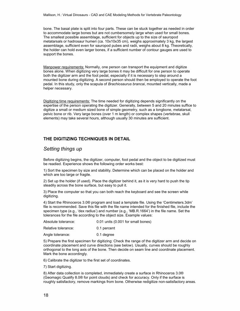
Setting things up Before digitizing begins, the digitizer, computer, foot pedal and the object to be digitized must be readied. Experience shows the following order works best:
1) Sort the specimen by size and stability. Determine which can be placed on the holder and which are too large or fragile.
2) Set up the holder (if used). Place the digitizer behind it, as it is very hard to push the tip steadily across the bone surface, but easy to pull it.
3) Place the computer so that you can both reach the keyboard and see the screen while digitizing.
4) Start the Rhinoceros 3.0® program and load a template file. Using the ‘Centimeters.3dm’ file is recommended. Save this file with the file name intended for the finished file, include the specimen type (e.g., ‘dex radius’) and number (e.g., ‘MB.R.1664’) in the file name. Set the tolerances for the file according to the object size. Example values:
Absolute tolerance: 0.01 units (0.001 for small bones)
Relative tolerance: 0.1 percent
Angle tolerance: 0.1 degree
5) Prepare the first specimen for digitizing: Check the range of the digitizer arm and decide on coordinate placement and curve directions (see below). Usually, curves should be roughly orthogonal to the long axis of the bone. Then decide on seam line and coordinate placement. Mark the bone accordingly.
6) Calibrate the digitizer to the first set of coordinates.
7) Start digitizing.
8) After data collection is completed, immediately create a surface in Rhinoceros 3.0® (Geomagic Qualify 8.0® for point clouds) and check for accuracy. Only if the surface is roughly satisfactory, remove markings from bone. Otherwise redigitize non-satisfactory areas.
Mallison, H.: Virtual Dinosaurs - CAD and CAE Modeling Methods for Vertebrate Paleontology
19
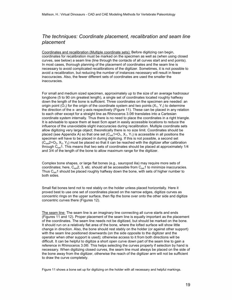
The techniques: Coordinate placement, recalibration and seam line placement Coordinates and recalibration (Multiple coordinate sets): Before digitizing can begin, coordinates for recalibration must be marked on the specimen as well as (when using closed curves, see below) a seam line (line through the contacts of all curves start and end points). In most cases, thorough planning of the placement of coordinates and the seam line is necessary to avoid complicated recalibrations of the digitizer. Sometimes, it is not possible to avoid a recalibration, but reducing the number of instances necessary will result in fewer inaccuracies. Also, the fewer different sets of coordinates are used the smaller the inaccuracies.
For small and medium sized specimen, approximately up to the size of an average hadrosaur longbone (5 to 90 cm greatest length), a single set of coordinates located roughly halfway down the length of the bone is sufficient. Three coordinates on the specimen are needed: an origin point (O1) for the origin of the coordinate system and two points (X1, Y1) to determine the direction of the x- and y-axis respectively (Figure 11). These can be placed in any relation to each other except for a straight line as Rhinoceros 3.0® translates into a Cartesian coordinate system internally. Thus there is no need to place the coordinates in a right triangle. It is advisable to space them at least 5cm apart in easily accessible locations to reduce the influence of the unavoidable slight inaccuracies during recalibration. Multiple coordinate sets allow digitizing very large object; theoretically there is no size limit. Coordinates should be placed (see Appendix A) so that one set (Cset1=O1, X1, Y1) is accessible in all positions the specimen will have to be placed in during digitizing. If this is not possible, a second set (Cset2=O2, X2, Y2) must be placed so that it can be reached with the digitizer after calibration through Cset1. This means that two sets of coordinates should be placed at approximately 1/4 and 3/4 of the length of the bone to allow maximum range for the digitizer.
Complex bone shapes, or large flat bones (e.g., sauropod ilia) may require more sets of coordinates; here, Cset2, 3, etc. should all be accessible from Cset1 to minimize inaccuracies. Thus Cset1 should be placed roughly halfway down the bone, with sets of higher number to both sides.
Small flat bones tend not to rest stably on the holder unless placed horizontally. Here it proved best to use one set of coordinates placed on the narrow edges, digitize curves as concentric rings on the upper surface, then flip the bone over onto the other side and digitize concentric curves there (Figures 12).
The seam line: The seam line is an imaginary line connecting all curve starts and ends (Figures 11 and 12). Proper placement of the seam line is equally important as the placement of the coordinates. The seam line needs not be digitized, but should be marked on the bone. It should run on a relatively flat area of the bone, where the lofted surface will show little change in direction. Also, the bone should rest stably on the holder (or against other support) with the seam line positioned downwards (on the side opposite to the digitizer and the operator when other support is used); otherwise access to it from both directions will be difficult. It can be helpful to digitize a short open curve down part of the seam line to gain a reference in Rhinoceros 3.0®. This helps selecting the curves properly if selection by hand is necessary. When digitizing closed curves, the seam line must always be placed on the side of the bone away from the digitizer, otherwise the reach of the digitizer arm will not be sufficient to draw the curve completely.
Figure 11 shows a bone set up for digitizing on the holder with all necessary and helpful markings.
Mallison, H.: Virtual Dinosaurs - CAD and CAE Modeling Methods for Vertebrate Paleontology
20
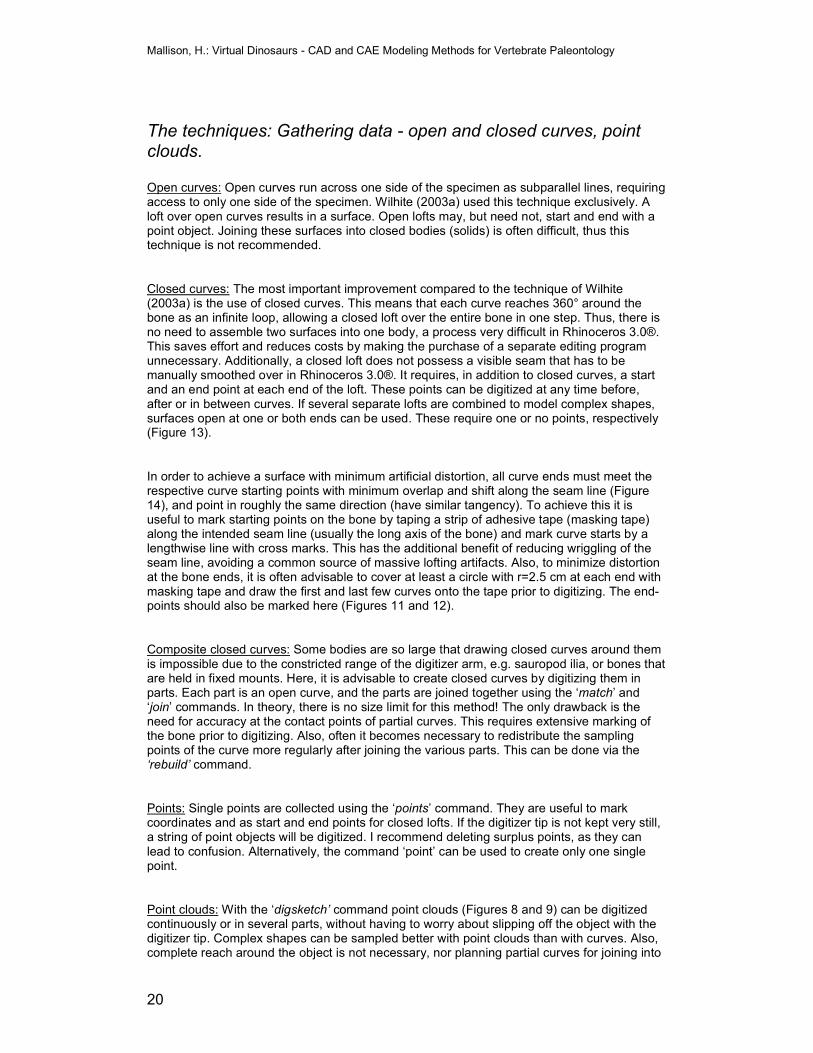
The techniques: Gathering data - open and closed curves, point clouds.
Open curves: Open curves run across one side of the specimen as subparallel lines, requiring access to only one side of the specimen. Wilhite (2003a) used this technique exclusively. A loft over open curves results in a surface. Open lofts may, but need not, start and end with a point object. Joining these surfaces into closed bodies (solids) is often difficult, thus this technique is not recommended.
Closed curves: The most important improvement compared to the technique of Wilhite (2003a) is the use of closed curves. This means that each curve reaches 360° around the bone as an infinite loop, allowing a closed loft over the entire bone in one step. Thus, there is no need to assemble two surfaces into one body, a process very difficult in Rhinoceros 3.0®. This saves effort and reduces costs by making the purchase of a separate editing program unnecessary. Additionally, a closed loft does not possess a visible seam that has to be manually smoothed over in Rhinoceros 3.0®. It requires, in addition to closed curves, a start and an end point at each end of the loft. These points can be digitized at any time before, after or in between curves. If several separate lofts are combined to model complex shapes, surfaces open at one or both ends can be used. These require one or no points, respectively (Figure 13).
In order to achieve a surface with minimum artificial distortion, all curve ends must meet the respective curve starting points with minimum overlap and shift along the seam line (Figure 14), and point in roughly the same direction (have similar tangency). To achieve this it is useful to mark starting points on the bone by taping a strip of adhesive tape (masking tape) along the intended seam line (usually the long axis of the bone) and mark curve starts by a lengthwise line with cross marks. This has the additional benefit of reducing wriggling of the seam line, avoiding a common source of massive lofting artifacts. Also, to minimize distortion at the bone ends, it is often advisable to cover at least a circle with r=2.5 cm at each end with masking tape and draw the first and last few curves onto the tape prior to digitizing. The end-points should also be marked here (Figures 11 and 12).
Composite closed curves: Some bodies are so large that drawing closed curves around them is impossible due to the constricted range of the digitizer arm, e.g. sauropod ilia, or bones that are held in fixed mounts. Here, it is advisable to create closed curves by digitizing them in parts. Each part is an open curve, and the parts are joined together using the ‘match’ and ‘join’ commands. In theory, there is no size limit for this method! The only drawback is the need for accuracy at the contact points of partial curves. This requires extensive marking of the bone prior to digitizing. Also, often it becomes necessary to redistribute the sampling points of the curve more regularly after joining the various parts. This can be done via the ‘rebuild’ command.
Points: Single points are collected using the ‘points’ command. They are useful to mark coordinates and as start and end points for closed lofts. If the digitizer tip is not kept very still, a string of point objects will be digitized. I recommend deleting surplus points, as they can lead to confusion. Alternatively, the command ‘point’ can be used to create only one single point.
Point clouds: With the ‘digsketch’ command point clouds (Figures 8 and 9) can be digitized continuously or in several parts, without having to worry about slipping off the object with the digitizer tip. Complex shapes can be sampled better with point clouds than with curves. Also, complete reach around the object is not necessary, nor planning partial curves for joining into
Mallison, H.: Virtual Dinosaurs - CAD and CAE Modeling Methods for Vertebrate Paleontology
21
closed ones. This is useful when bones are mounted closely together and can not be taken off the mount for digitizing.
The object is placed on a stable support, e.g. placed in a sandbox. Coordinates must be marked so that they are accessible in all positions necessary for digitizing the complete bone. Now point clouds are digitized over the entire accessible surface. Then the object is turned over, the digitizer recalibrated and the remaining surfaces are digitized. Experience tells that drawing the digitizer tip along all edges is advisable; larger flat areas can be painted in roughly with a to and fro movement of the digitizer. Note that near sharp edges, such as cristae or the edges of transverse processes, artifacts will appear near the edges of the flat surfaces if the sampling distance on the surface is not significantly smaller than the thickness of the bone. Meshing then erroneously connects points from both sides to each other instead of to the points at the edge (Figure 9). The sampling distance should be at most 0.2 times the distance of the surfaces to avoid this. During digitizing, it is advisable to create meshes from time to time in order to judge which areas need further digitizing. It is also possible to digitize with this preliminary mesh visible, best in ‘Shaded’ viewport mode, which facilitates the task. Alternative, the mesh can be created in Geomagic Qualify 8.0®, as Rhinoceros 3.0® will accept digitizer input even if it is running as a background process.
Although curves for lofting can be created from these points by a variety of methods, using the ‘wrap’ function in Geomagic Qualify 8.0® usually is the best option to create a polygon mesh. If some areas prove troublesome, separate meshes can be created for parts of the point cloud and then combined. The gaps can be filled with the ‘FillHoles’ function of Geomagic Qualify 8.0®.
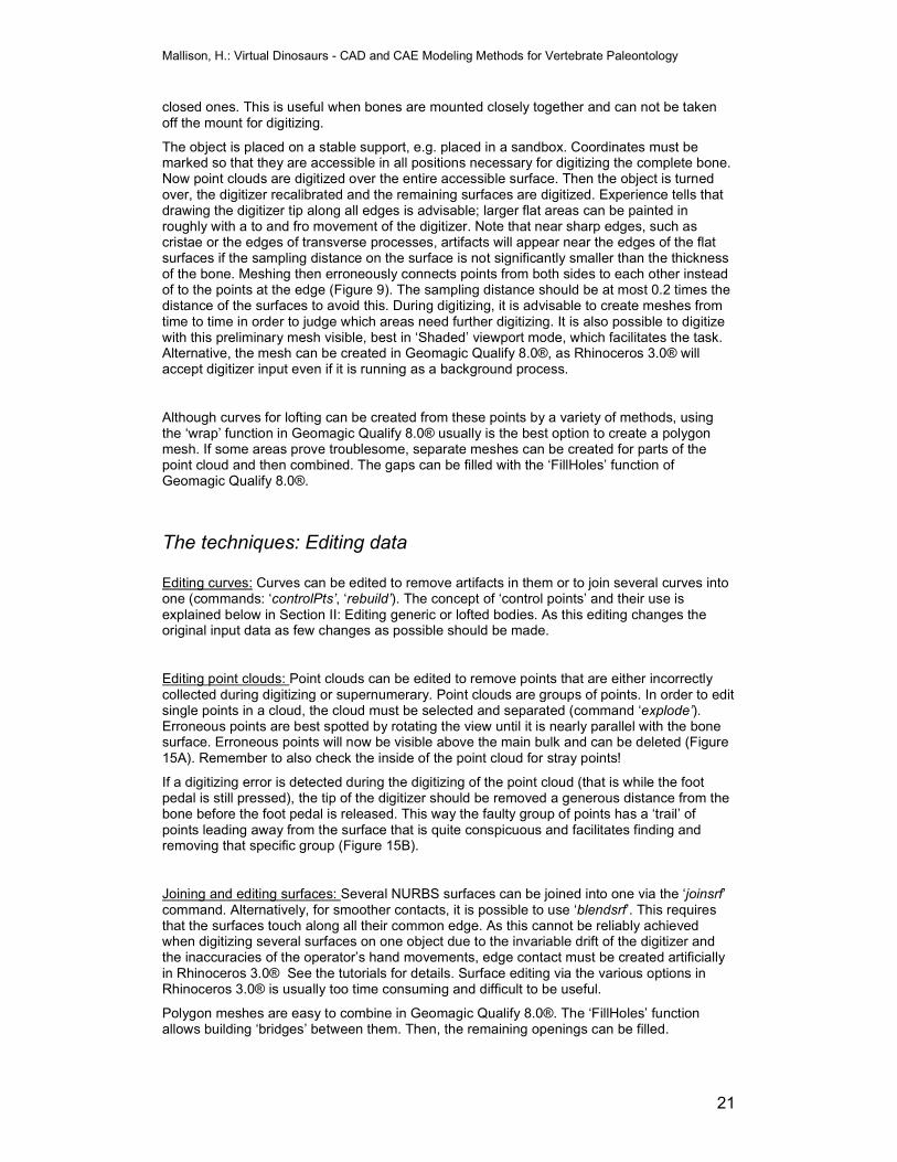
The techniques: Editing data
Editing curves: Curves can be edited to remove artifacts in them or to join several curves into one (commands: ‘controlPts’, ‘rebuild’). The concept of ‘control points’ and their use is explained below in Section II: Editing generic or lofted bodies. As this editing changes the original input data as few changes as possible should be made.
Editing point clouds: Point clouds can be edited to remove points that are either incorrectly collected during digitizing or supernumerary. Point clouds are groups of points. In order to edit single points in a cloud, the cloud must be selected and separated (command ‘explode’). Erroneous points are best spotted by rotating the view until it is nearly parallel with the bone surface. Erroneous points will now be visible above the main bulk and can be deleted (Figure 15A). Remember to also check the inside of the point cloud for stray points!
If a digitizing error is detected during the digitizing of the point cloud (that is while the foot pedal is still pressed), the tip of the digitizer should be removed a generous distance from the bone before the foot pedal is released. This way the faulty group of points has a ‘trail’ of points leading away from the surface that is quite conspicuous and facilitates finding and removing that specific group (Figure 15B).
Joining and editing surfaces: Several NURBS surfaces can be joined into one via the ‘joinsrf’ command. Alternatively, for smoother contacts, it is possible to use ‘blendsrf’. This requires that the surfaces touch along all their common edge. As this cannot be reliably achieved when digitizing several surfaces on one object due to the invariable drift of the digitizer and the inaccuracies of the operator’s hand movements, edge contact must be created artificially in Rhinoceros 3.0® See the tutorials for details. Surface editing via the various options in Rhinoceros 3.0® is usually too time consuming and difficult to be useful.
Polygon meshes are easy to combine in Geomagic Qualify 8.0®. The ‘FillHoles’ function allows building ‘bridges’ between them. Then, the remaining openings can be filled.
Mallison, H.: Virtual Dinosaurs - CAD and CAE Modeling Methods for Vertebrate Paleontology
22
The techniques: Creating bodies - lofting and joining surfaces
Surfaces from curves: Lofting a surface over closed curves (command ‘loft’) is the easiest way to create surfaces for digitized objects in Rhinoceros 3.0®. A loft that, in addition to the curves, contains a point object at one end will be closed at that end, but still be a surface, not a body. A loft that both starts and ends with a point will create a body, not a surface. This method requires the least post-digitizing data editing. In order to loft, the respective curves must be selected and the proper loft option chosen. Usually, Rhinoceros 3.0® does not reliably sort curves correctly, so each point/curve must be selected by hand in the proper order, starting with one endpoint, then the closest curve, then the next etc. to the other end of the bone. In Rhinoceros 2.0 and earlier version, each curve has a direction that does not get automatically adjusted during lofting. It is necessary to select each curve at the same side of the seam line; otherwise the surface will fold into itself. Rhinoceros 3.0® sorts the directions automatically.
Note that large bones digitized at high accuracy will lead to long computation times for lofting. It may be advisable to increase tolerances in the file preferences before lofting, as this will not add a significant error but speed up lofting by up to 90%. Additionally, I have experienced program crashes at high accuracies, which can be avoided by downgrading the accuracy values after data collection and before lofting.
Surfaces from point clouds: Meshing is done automatically via the ‘Meshfrompoints’ command in Rhinoceros 3.0®. Much more accurate results can be achieved in Geomagic Qualify 8.0®, using the ‘Wrap’ function. If the resulting mesh shows many inaccuracies, deleting it and editing the point cloud for a new meshing is best. If there are few errors in the created surface, it is best to delete erroneous mesh facets (‘Deletemeshfaces’) and fill the resulting holes via the ‘fillhole’ command in Rhinoceros 3.0®. In Geomagic Qualify 8.0®, faulty areas can be selected directly and removed by pressing ‘Del’. The holes can be filled using the ‘FillHoles’ function.
In Rhinoceros 3.0®, tolerance settings should remain tight for meshing, as low values will result in significant errors.
APPLICATIONS OF TECHNIQUES TO DIFFERENT SPECIMEN TYPES
Digitizing with closed curves – general remarks
Plan coordinate and seam line position prior to digitizing and mark them. Keep the limited range of the digitizer arm in mind! When aiming for a closed loft, remember to digitize start and end points! Closed curves may lead to artifacts, usually along the seam line or in places where neighboring curves are of significantly different lengths or their distance and direction varies greatly. The same is true if closed curves overlap or shift at the seam line. Here, using the ‘Simplify: Rebuild…’ option of the ‘loft’ command dialog box can reduce or remove the problem. Alternatively, the curves can be edited prior to lofting via the ‘rebuild’ command, or by editing their ‘control points’. See Appendix A and Section II: ‘Editing generic or lofted bodies’ for details on these options, respectively.
Digitizing with closed curves – small bones (simple shapes) Small bones (5 to 20 cm maximum length) tend to be hard to digitize for a number of reasons. They shift position easily, drawing curves on or around them at relatively regular intervals without overlap alone is hard, and ensuring that these curves accurately reproduce small
Mallison, H.: Virtual Dinosaurs - CAD and CAE Modeling Methods for Vertebrate Paleontology
23
surface features makes the task of drawing curves free-handed too cumbersome. Using the fossil holder reduces the first problem. Still, care must be taken not to put pressure on the specimen with the tip of the digitizer as this may shift the bone. As it is hard to place a small bone on the holder stably while still being able to reach both upper and lower surfaces, the author recommends first digitizing only the upper half with concentric closed curves in a horizontal plane, then flipping the bone over and repeating the procedure for the other half. This requires a coordinate set Cset1 placed on the circumference of the bone (Figure 12).
The problem of drawing curves properly - especially closed curves - can be solved by extensive marking of the bone. For this, much or all of the bone is covered in painter’s adhesive tape or masking tape and the seam line and curves are drawn onto it (Figure 12). It is also possible to only mark partial curves or markers for curve passage over radially placed strips of tape if the bone is too large for complete wrapping. It is of paramount important to select a tape that can be removed without damaging the bone.
Digitizing with closed curves – medium sized bones For medium sized elements (up to around 90 cm maximum length), curves should be placed perpendicularly to the long axis of the bone, with the seam line on the lower side. The specially constructed holder again proved best, as it keeps the specimen from shifting while allowing easy access. Usually, it will not prevent access to important features and curves placed directly to the left and right of the fittings are sufficient to give an accurate surface. If not, it is necessary to shift the bone a few centimeters and recalibrate the digitizer before adding curves into the gaps. See Figure 11 for an example of this setup.
Digitizing with closed curves – large bones Drawing closed curves requires that it is possible to reach around the specimen on both sides down to the seam line. For very large specimens, especially relatively slender longbones like tibiae and radii of sauropods, it is advisable to place the specimen close to vertical by leaning it against a solid structure, with a cut-to-fit styrofoam spacer to create a gap in between (Figure 16). Some bones, especially sauropod longbones, rest stably in this position on their articular ends. If necessary, the lower end can be secured with wooden wedges and small sandbags or in a sandbox. Thus bending moments on the shaft are minimal. The digitizer may have to be set up on a wooden box or a chair in front of the bone to achieve a sufficient vertical reach; care must be given to stability. This allows digitizing the top end and shaft with curves parallel to the ground; then the fossil must be turned upside down, the digitizer recalibrated and the bottom end added. The seam line here runs down the ‘back’ of the bone, opposite the digitizer and operator. In early versions of Rhinoceros®, care must be given to either digitize the curves in the opposite direction after rotating the specimen (seam line now at front) or change curve direction in Rhinoceros 3.0® before or during lofting.
Digitizing with composite closed curves (very large bones and/or complex bone shapes) Bones that are too large in circumfence for closed curves or encased in supports that make reaching around them impossible can be digitized by drawing sets of open curves. Each curve in a set ends at the starting point of a curve from another set. Two or more curves together must fully surround the bone the way a closed curve would. This requires extensive marking of the bone to minimize overlap and shift between touching curves. It is advisable to place the contact line between curves at places with low curvature (i.e. flat bone surfaces) to minimize artifacts and leave a very small gap between curves. The partial curves then must
Mallison, H.: Virtual Dinosaurs - CAD and CAE Modeling Methods for Vertebrate Paleontology
24
be joined into closed curves using the ‘match’ and ‘join’ commands. Then, a closed loft can be made over the entire bone.
Usually, it is necessary to rebuild matched curves using the ‘rebuild‘ command to avoid artifacts, as the control points will be unevenly distributed along each curve.
Digitizing bones as composite bodies with separate curve sets - complex bone shapes
Some bones possess shapes that cannot be represented by one loft over closed curves. In these cases, it is possible to digitize parts of the bone, loft surfaces over these parts, and then combine them into one body in Rhinoceros 3.0®. Examples are the articular heads of sauropod ribs, where one set of closed curves cannot easily be drawn around both heads. Digitizing as large a part as possible with curves in one direction, then adding a second set of curves for the missing parts is usually the best option, although it is sometimes preferable to aim to minimize the suture length between the parts.
Several points must be kept in mind when planning a composite body:
- The separate parts must together contain the entire surface or volume of the specimen when using open surfaces or closed surfaces, respectively; otherwise there will be gaps or holes. If holes cannot be avoided, they should be in flat areas of the bone, where filling them up in Rhinoceros 3.0® is easy and carries a low risk of error.
- The separate lofts must overlap enough or contact each other exactly to allow joining the bodies in Rhinoceros 3.0®.
- The overlap area should not contain repeat intersections between surfaces/bodies as these tend to confuse Rhinoceros 3.0® and make merging impossible. It is helpful to close lofted bodies by placing the end point inside the bone by manually adding it in Rhinoceros 3.0®. This guarantees overlap with only one section contact.
- It is advisable to digitize a closed curve along the contact line of the parts to be joined. This facilitates creation of a cutting plane, which allows cropping the parts to an exact fit.
- To create holes in a body (e.g., foramina in ischia or coracoids) it can be easier to digitize and loft an air volume and subtract it from the main body than splitting the main body into parts and joining them.
- Remember to set the tolerances tight enough, otherwise cutting and joining surfaces may not work properly.
Using open curves and multiple lofts: A closed curve should additionally be digitized along each suture line to facilitate closing each open loft into a closed body before joining the adjacent bodies.
Using closed curves and multiple lofts: A closed curve should additionally be digitized along each suture line to facilitate cropping both adjacent bodies to avoid problems when joining them.
When it is not possible to digitize one closed curve around the end of the surface it is possible to digitize it in parts, and then join them into one curve using the ‘match’ command.
Mallison, H.: Virtual Dinosaurs - CAD and CAE Modeling Methods for Vertebrate Paleontology
25
Digitizing with point clouds/meshes (small bones with complex shapes, partially inaccessible bones) Any bone too small to rest stably on the holder and with a shape too complex to be easily digitized by the above method for small bones using closed curves should be placed either on clay or in a sandbox. The ‘Digsketch’ command allows collection of point clouds. Care must be taken to ensure that the distance between closest points on the same surface is always significantly smaller than the distance to points on any other surface; otherwise artifacts will be produced during meshing. ‘Meshfrompoints’ produces a polygon mesh that can be edited via the ‘deletemeshfaces’ and ‘fillhole’ commands. Reducing the mesh count in Rhinoceros 3.0® is usually not advisable, as the errors incurred are significant. Both meshing and editing of the mesh are better carried out in Geomagic Qualify 8.0 (see Appendix B). This is especially true for filling gaps in the mesh.
Theoretically, Geomagic Qualify 8.0 also supports the Microscribe 3D digitizer. For unknown reasons, the author was not able to make the digitizer connect to the program correctly. Despite this technical problem, Geomagic Qualify 8.0 can be a helpful tool during digitizing of point clouds: It is possible to collect data with the digitizer in Rhinoceros 3.0® while the other program is displayed on the screen. Therefore, one can digitize points in Rhinoceros 3.0®, intermittently mesh them in Geomagic Qualify 8.0® and then go on collecting data to fill the gaps shown in the mesh in Rhinoceros 3.0® while the mesh is actually visible on the screen. Due to the far better ability to selectively collect data where it is needed, this process can save up to 30% of the digitizing time. Also, errors will show up earlier, allowing faster correction.
Marking surface features Rugosities, damaged or discolored areas, articular surfaces or muscle attachment scars can be marked on the surface by drawing a closed curve around them. This curve can later be projected onto the lofted surface. While this data will usually be lost when exporting the 3D bodies into other programs, some formats allow retention. Also, a very thin body can be constructed from the curve via the ‘extrude’ command; this will be preserved in all formats. Rhinoceros 3.0® allows changing the color of these markings to make them more conspicuous. Alternatively, the area can be covered with a point cloud, from which a polygon mesh can be created.
Composite bones from partially preserved specimens Here, an example is given for combining two parts; a higher number can be combined by repetition. There are two methods for combining data from two specimens. It is possible to select at least three landmarks, which are present on both objects, and digitize them as coordinates for a coordinate system, then digitize the specimens after calibrating to these landmarks. This works well if there are e.g. small foramina or sutural contacts with ontogenetically stable positions present on the bones. Optimally, only one set of closed curves is needed, with the last curve of one specimen subparallel to the first of the second specimen.
If no landmarks are present, it is possible to just digitize the specimen without calibrating from one to the other, then copy and paste them into one file and move one until it appears to fit the other. This process works well if there are cristae or spinae present, or any other feature on the bone that allows easy 3D orientation of the separate parts. For both methods it is possible to scale (‘scale’ command) one part to fit the other. In any case, a note should be added to the file indicating the composite nature of the model.
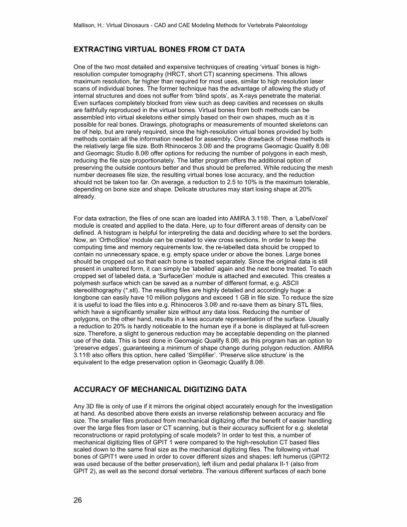
Mallison, H.: Virtual Dinosaurs - CAD and CAE Modeling Methods for Vertebrate Paleontology
26
EXTRACTING VIRTUAL BONES FROM CT DATA
One of the two most detailed and expensive techniques of creating ‘virtual’ bones is high-resolution computer tomography (HRCT, short CT) scanning specimens. This allows maximum resolution, far higher than required for most uses, similar to high resolution laser scans of individual bones. The former technique has the advantage of allowing the study of internal structures and does not suffer from ‘blind spots’, as X-rays penetrate the material. Even surfaces completely blocked from view such as deep cavities and recesses on skulls are faithfully reproduced in the virtual bones. Virtual bones from both methods can be assembled into virtual skeletons either simply based on their own shapes, much as it is possible for real bones. Drawings, photographs or measurements of mounted skeletons can be of help, but are rarely required, since the high-resolution virtual bones provided by both methods contain all the information needed for assembly. One drawback of these methods is the relatively large file size. Both Rhinoceros 3.0® and the programs Geomagic Qualify 8.0® and Geomagic Studio 8.0® offer options for reducing the number of polygons in each mesh, reducing the file size proportionately. The latter program offers the additional option of preserving the outside contours better and thus should be preferred. While reducing the mesh number decreases file size, the resulting virtual bones lose accuracy, and the reduction should not be taken too far. On average, a reduction to 2.5 to 10% is the maximum tolerable, depending on bone size and shape. Delicate structures may start losing shape at 20% already.
For data extraction, the files of one scan are loaded into AMIRA 3.11®. Then, a ‘LabelVoxel’ module is created and applied to the data. Here, up to four different areas of density can be defined. A histogram is helpful for interpreting the data and deciding where to set the borders. Now, an ‘OrthoSlice’ module can be created to view cross sections. In order to keep the computing time and memory requirements low, the re-labelled data should be cropped to contain no unnecessary space, e.g. empty space under or above the bones. Large bones should be cropped out so that each bone is treated separately. Since the original data is still present in unaltered form, it can simply be ‘labelled’ again and the next bone treated. To each cropped set of labeled data, a ‘SurfaceGen’ module is attached and executed. This creates a polymesh surface which can be saved as a number of different format, e.g. ASCII stereolithography (*.stl). The resulting files are highly detailed and accordingly huge: a longbone can easily have 10 million polygons and exceed 1 GB in file size. To reduce the size it is useful to load the files into e.g. Rhinoceros 3.0® and re-save them as binary STL files, which have a significantly smaller size without any data loss. Reducing the number of polygons, on the other hand, results in a less accurate representation of the surface. Usually a reduction to 20% is hardly noticeable to the human eye if a bone is displayed at full-screen size. Therefore, a slight to generous reduction may be acceptable depending on the planned use of the data. This is best done in Geomagic Qualify 8.0®, as this program has an option to ‘preserve edges’, guaranteeing a minimum of shape change during polygon reduction. AMIRA 3.11® also offers this option, here called ‘Simplifier’. ‘Preserve slice structure’ is the equivalent to the edge preservation option in Geomagic Qualify 8.0®.
ACCURACY OF MECHANICAL DIGITIZING DATA
Any 3D file is only of use if it mirrors the original object accurately enough for the investigation at hand. As described above there exists an inverse relationship between accuracy and file size. The smaller files produced from mechanical digitizing offer the benefit of easier handling over the large files from laser or CT scanning, but is their accuracy sufficient for e.g. skeletal reconstructions or rapid prototyping of scale models? In order to test this, a number of mechanical digitizing files of GPIT 1 were compared to the high-resolution CT based files scaled down to the same final size as the mechanical digitizing files. The following virtual bones of GPIT1 were used in order to cover different sizes and shapes: left humerus (GPIT2 was used because of the better preservation), left ilium and pedal phalanx II-1 (also from GPIT 2), as well as the second dorsal vertebra. The various different surfaces of each bone
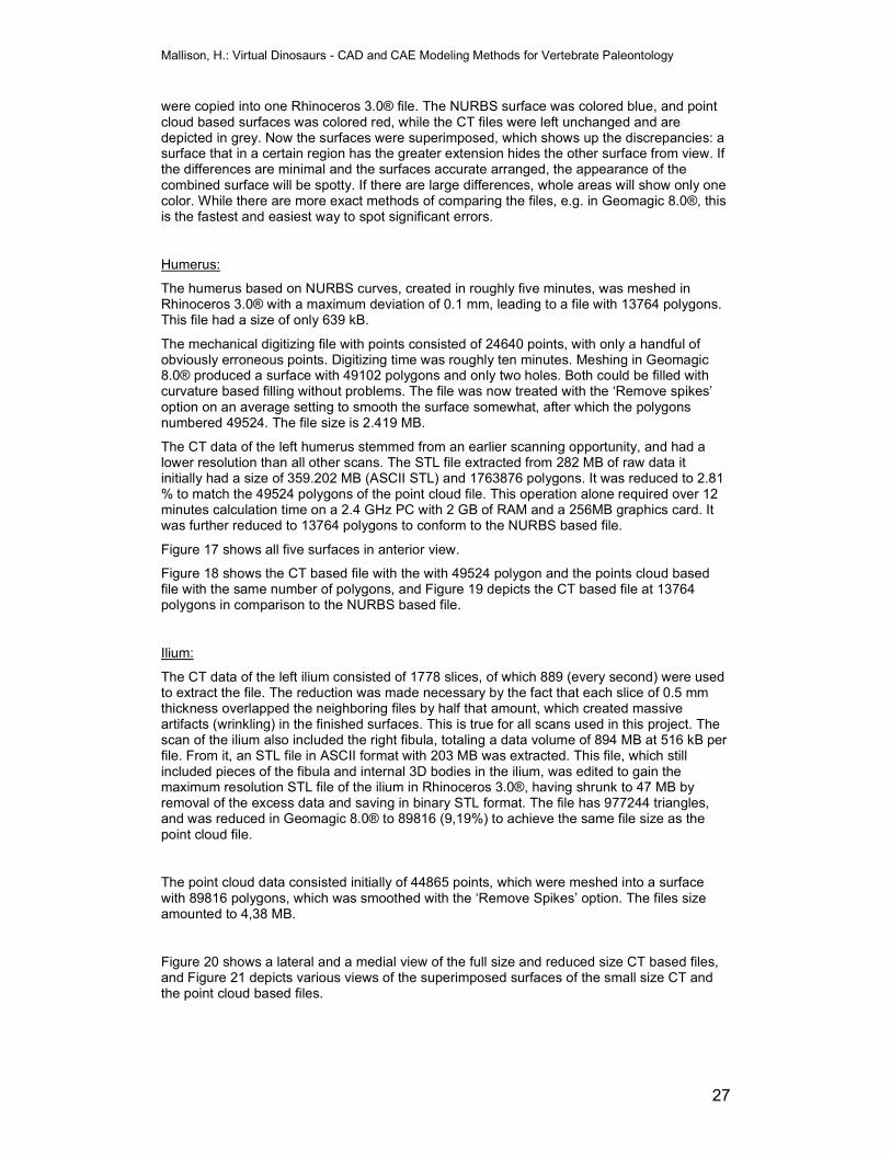
Mallison, H.: Virtual Dinosaurs - CAD and CAE Modeling Methods for Vertebrate Paleontology
27
were copied into one Rhinoceros 3.0® file. The NURBS surface was colored blue, and point cloud based surfaces was colored red, while the CT files were left unchanged and are depicted in grey. Now the surfaces were superimposed, which shows up the discrepancies: a surface that in a certain region has the greater extension hides the other surface from view. If the differences are minimal and the surfaces accurate arranged, the appearance of the combined surface will be spotty. If there are large differences, whole areas will show only one color. While there are more exact methods of comparing the files, e.g. in Geomagic 8.0®, this is the fastest and easiest way to spot significant errors.
Humerus:
The humerus based on NURBS curves, created in roughly five minutes, was meshed in Rhinoceros 3.0® with a maximum deviation of 0.1 mm, leading to a file with 13764 polygons. This file had a size of only 639 kB.
The mechanical digitizing file with points consisted of 24640 points, with only a handful of obviously erroneous points. Digitizing time was roughly ten minutes. Meshing in Geomagic 8.0® produced a surface with 49102 polygons and only two holes. Both could be filled with curvature based filling without problems. The file was now treated with the ‘Remove spikes’ option on an average setting to smooth the surface somewhat, after which the polygons numbered 49524. The file size is 2.419 MB.
The CT data of the left humerus stemmed from an earlier scanning opportunity, and had a lower resolution than all other scans. The STL file extracted from 282 MB of raw data it initially had a size of 359.202 MB (ASCII STL) and 1763876 polygons. It was reduced to 2.81 % to match the 49524 polygons of the point cloud file. This operation alone required over 12 minutes calculation time on a 2.4 GHz PC with 2 GB of RAM and a 256MB graphics card. It was further reduced to 13764 polygons to conform to the NURBS based file.
Figure 17 shows all five surfaces in anterior view.
Figure 18 shows the CT based file with the with 49524 polygon and the points cloud based file with the same number of polygons, and Figure 19 depicts the CT based file at 13764 polygons in comparison to the NURBS based file.
Ilium:
The CT data of the left ilium consisted of 1778 slices, of which 889 (every second) were used to extract the file. The reduction was made necessary by the fact that each slice of 0.5 mm thickness overlapped the neighboring files by half that amount, which created massive artifacts (wrinkling) in the finished surfaces. This is true for all scans used in this project. The scan of the ilium also included the right fibula, totaling a data volume of 894 MB at 516 kB per file. From it, an STL file in ASCII format with 203 MB was extracted. This file, which still included pieces of the fibula and internal 3D bodies in the ilium, was edited to gain the maximum resolution STL file of the ilium in Rhinoceros 3.0®, having shrunk to 47 MB by removal of the excess data and saving in binary STL format. The file has 977244 triangles, and was reduced in Geomagic 8.0® to 89816 (9,19%) to achieve the same file size as the point cloud file.
The point cloud data consisted initially of 44865 points, which were meshed into a surface with 89816 polygons, which was smoothed with the ‘Remove Spikes’ option. The files size amounted to 4,38 MB.
Figure 20 shows a lateral and a medial view of the full size and reduced size CT based files, and Figure 21 depicts various views of the superimposed surfaces of the small size CT and the point cloud based files.
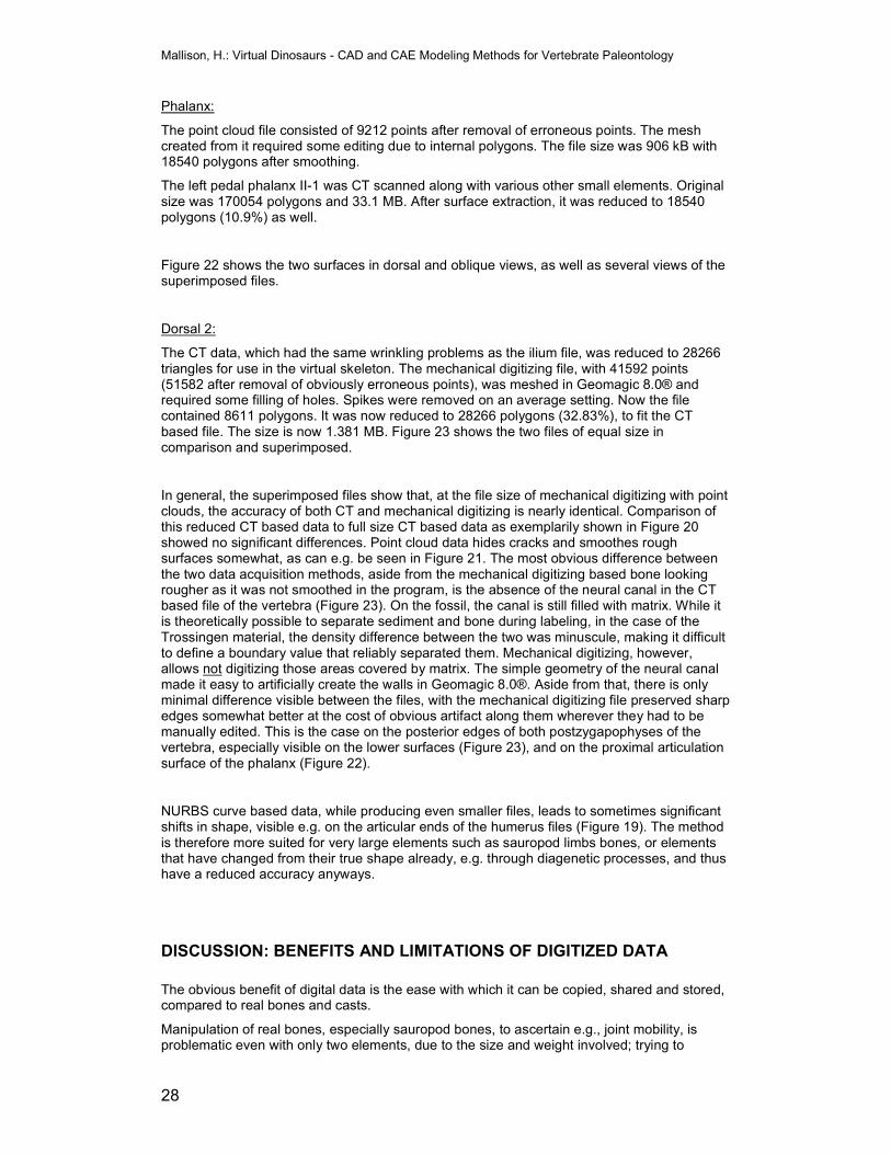
Mallison, H.: Virtual Dinosaurs - CAD and CAE Modeling Methods for Vertebrate Paleontology
28
Phalanx:
The point cloud file consisted of 9212 points after removal of erroneous points. The mesh created from it required some editing due to internal polygons. The file size was 906 kB with 18540 polygons after smoothing.
The left pedal phalanx II-1 was CT scanned along with various other small elements. Original size was 170054 polygons and 33.1 MB. After surface extraction, it was reduced to 18540 polygons (10.9%) as well.
Figure 22 shows the two surfaces in dorsal and oblique views, as well as several views of the superimposed files.
Dorsal 2:
The CT data, which had the same wrinkling problems as the ilium file, was reduced to 28266 triangles for use in the virtual skeleton. The mechanical digitizing file, with 41592 points (51582 after removal of obviously erroneous points), was meshed in Geomagic 8.0® and required some filling of holes. Spikes were removed on an average setting. Now the file contained 8611 polygons. It was now reduced to 28266 polygons (32.83%), to fit the CT based file. The size is now 1.381 MB. Figure 23 shows the two files of equal size in comparison and superimposed.
In general, the superimposed files show that, at the file size of mechanical digitizing with point clouds, the accuracy of both CT and mechanical digitizing is nearly identical. Comparison of this reduced CT based data to full size CT based data as exemplarily shown in Figure 20 showed no significant differences. Point cloud data hides cracks and smoothes rough surfaces somewhat, as can e.g. be seen in Figure 21. The most obvious difference between the two data acquisition methods, aside from the mechanical digitizing based bone looking rougher as it was not smoothed in the program, is the absence of the neural canal in the CT based file of the vertebra (Figure 23). On the fossil, the canal is still filled with matrix. While it is theoretically possible to separate sediment and bone during labeling, in the case of the Trossingen material, the density difference between the two was minuscule, making it difficult to define a boundary value that reliably separated them. Mechanical digitizing, however, allows not digitizing those areas covered by matrix. The simple geometry of the neural canal made it easy to artificially create the walls in Geomagic 8.0®. Aside from that, there is only minimal difference visible between the files, with the mechanical digitizing file preserved sharp edges somewhat better at the cost of obvious artifact along them wherever they had to be manually edited. This is the case on the posterior edges of both postzygapophyses of the vertebra, especially visible on the lower surfaces (Figure 23), and on the proximal articulation surface of the phalanx (Figure 22).
NURBS curve based data, while producing even smaller files, leads to sometimes significant shifts in shape, visible e.g. on the articular ends of the humerus files (Figure 19). The method is therefore more suited for very large elements such as sauropod limbs bones, or elements that have changed from their true shape already, e.g. through diagenetic processes, and thus have a reduced accuracy anyways.
DISCUSSION: BENEFITS AND LIMITATIONS OF DIGITIZED DATA
The obvious benefit of digital data is the ease with which it can be copied, shared and stored, compared to real bones and casts.
Manipulation of real bones, especially sauropod bones, to ascertain e.g., joint mobility, is problematic even with only two elements, due to the size and weight involved; trying to
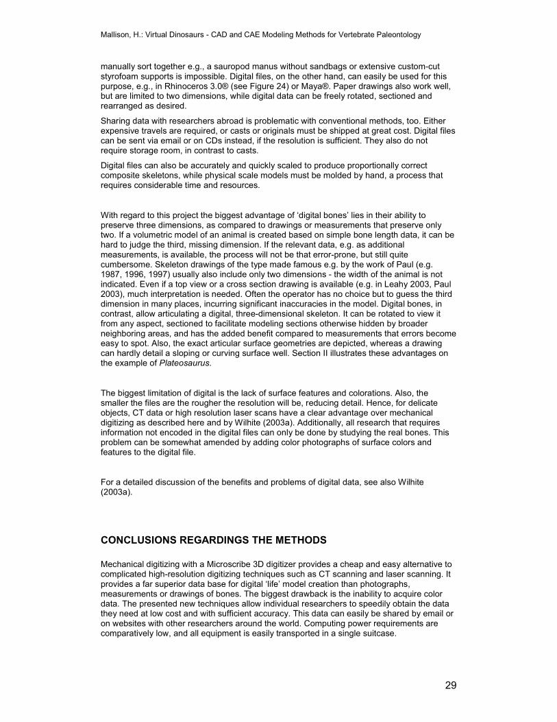
Mallison, H.: Virtual Dinosaurs - CAD and CAE Modeling Methods for Vertebrate Paleontology
29
manually sort together e.g., a sauropod manus without sandbags or extensive custom-cut styrofoam supports is impossible. Digital files, on the other hand, can easily be used for this purpose, e.g., in Rhinoceros 3.0® (see Figure 24) or Maya®. Paper drawings also work well, but are limited to two dimensions, while digital data can be freely rotated, sectioned and rearranged as desired.
Sharing data with researchers abroad is problematic with conventional methods, too. Either expensive travels are required, or casts or originals must be shipped at great cost. Digital files can be sent via email or on CDs instead, if the resolution is sufficient. They also do not require storage room, in contrast to casts.
Digital files can also be accurately and quickly scaled to produce proportionally correct composite skeletons, while physical scale models must be molded by hand, a process that requires considerable time and resources.
With regard to this project the biggest advantage of ‘digital bones’ lies in their ability to preserve three dimensions, as compared to drawings or measurements that preserve only two. If a volumetric model of an animal is created based on simple bone length data, it can be hard to judge the third, missing dimension. If the relevant data, e.g. as additional measurements, is available, the process will not be that error-prone, but still quite cumbersome. Skeleton drawings of the type made famous e.g. by the work of Paul (e.g. 1987, 1996, 1997) usually also include only two dimensions - the width of the animal is not indicated. Even if a top view or a cross section drawing is available (e.g. in Leahy 2003, Paul 2003), much interpretation is needed. Often the operator has no choice but to guess the third dimension in many places, incurring significant inaccuracies in the model. Digital bones, in contrast, allow articulating a digital, three-dimensional skeleton. It can be rotated to view it from any aspect, sectioned to facilitate modeling sections otherwise hidden by broader neighboring areas, and has the added benefit compared to measurements that errors become easy to spot. Also, the exact articular surface geometries are depicted, whereas a drawing can hardly detail a sloping or curving surface well. Section II illustrates these advantages on the example of Plateosaurus.
The biggest limitation of digital is the lack of surface features and colorations. Also, the smaller the files are the rougher the resolution will be, reducing detail. Hence, for delicate objects, CT data or high resolution laser scans have a clear advantage over mechanical digitizing as described here and by Wilhite (2003a). Additionally, all research that requires information not encoded in the digital files can only be done by studying the real bones. This problem can be somewhat amended by adding color photographs of surface colors and features to the digital file.
For a detailed discussion of the benefits and problems of digital data, see also Wilhite (2003a).
CONCLUSIONS REGARDINGS THE METHODS
Mechanical digitizing with a Microscribe 3D digitizer provides a cheap and easy alternative to complicated high-resolution digitizing techniques such as CT scanning and laser scanning. It provides a far superior data base for digital ‘life’ model creation than photographs, measurements or drawings of bones. The biggest drawback is the inability to acquire color data. The presented new techniques allow individual researchers to speedily obtain the data they need at low cost and with sufficient accuracy. This data can easily be shared by email or on websites with other researchers around the world. Computing power requirements are comparatively low, and all equipment is easily transported in a single suitcase.
Mallison, H.: Virtual Dinosaurs - CAD and CAE Modeling Methods for Vertebrate Paleontology
30
Three-dimensional digital files can be used for a wide variety of research studies, including ontogenetic and biomechanical aspects (see Section III), and are useful for museum display and curatorial aspects. However, data from mechanical digitizing is limited to reproduction of the general shape of bones, not high resolution surface detail. Also, post-digitizing file editing can consume additional time. These factors should be kept in mind before projects based on mechanically digitized data are planned.
APPLICATION IN THIS STUDY
Digitized material of Plateosaurus An almost complete individual of Plateosaurus engelhardti at the Institute for Geosciences, Tübingen University (GPIT 1) was CT scanned at the Radiologische Klinik of the Universitätsklinik Tübingen by Dr. med. Ludescher. The data was exported as DICOM files. Per scan, as many bones were scanned simultaneously as could be fitted into the CT scanner’s width, which can scan a 50 cm wide field. Figure 25 shows a topograph view as produced by the scanner software of a typical scan. In order to keep the cooling time between scans low and produce data sets small enough for AMIRA 3.11® to handle, scan length was limited to around 60 cm where possible. Longer scan were extensions used only if single bones exceeded a length of 60 cm (scapulae, femora). The polymesh files (*.stl ASCII format) produced in AMIRA 3.11® were loaded in Rhinoceros 3.0®. Unwanted mesh parts were removed and each bones saved as a separate binary STL file. These have the advantage of much smaller file size compared to ASCII STLs. In Geomagic Qualify 8.0®, the files were edited to remove meshing errors and to reduce the polygon count, usually to roughly 10% for small bones and 5% for longbones and pectoral or pelvic girdle elements. The manus and pedes of GPIT1 are not well preserved, they miss several elements. These were replaced by scanning the sinistral manus and pes of GPIT2. Dextral elements were produced by mirroring the better preserved sinistral ones. Since GPIT1 misses the skull and mandible, the skull of SMNS 13200 was scanned to complete the skeleton.
Other genera and objects
Additionally, a hand and foot of Diplodocus carnegii from the IFGT was CT scanned and the data extracted. Mechanical digitizing (NURBS surfaces) was used to digitize the same hand and foot of Diplodocus for comparison.
NURBS files were also created from a number of limb bones and girdle bones of the hadrosaur Brachylophosaurus canadensis from various specimens at the JRDI. The sinistral scapula, complete sinistral forelimb and the dextral hindlimb minus the femur of ‘Bertha’, a probable diplodocid found with the limbs embedded vertically in the sediment, were digitized at the PMG. The unusual taphonomy means that there is hardly any distortion visible in the bones, as they were stressed in their strongest and not, as usual, their weakest direction. They do not show the collapse of the marrow cavity common in sauropod longbones. At the MNHB, a complete sinistral pes and various limb and girdle elements of Barosaurus africanus, limb bones and girdle elements of Dicraeosaurus sattleri, a nearly complete manus of Brachiosaurus brancai and various girdle elements and limb bones from the collection as well as the mounted skeleton were digitized.
Also as point clouds, a toy models produced by Bullyland™ was digitized: a model of Plateosaurus produced under the scientific guidance of the SMNS.
Mallison, H.: Virtual Dinosaurs - CAD and CAE Modeling Methods for Vertebrate Paleontology
31
SECTION II
INTRODUCTION TO SECTION II
Images, whether they are photographs, drawings or digital models, have an ‘inherent’ truth of their own: we tend to emotionally believe them to be true before reflecting on their probability. In opposition to this, the spoken word or a written text is considered rationally. We tend to instinctively believe drawings or physical objects such as scale models to be ‘correct’, even if there are distinct differences from the true object. Unless one is given the option to directly compare the image with the original, one tends to underestimate discrepancies, while at the same time the image is also remembered in the future as a base against which to check new impressions. This way, small errors may escape detection almost forever, and will in fact hinder correct judgment of later impressions, so much so that correct details will be labeled ‘wrong’. Well-known images, those we are accustomed to, become ‘true’ in our perception, while anything different is instinctively doubted, sometimes even if it is presented in any equally believable format. This explains why dinosaur reconstruction drawings invariably appear to be ‘better’ to most people if they follow more mammalian patterns, which most people are well used to, than reptilian patterns, which few people are well accustomed with. A case in point is the shape of the thigh, which in those pictures instinctively considered ‘correct’ usually has a typical mammalian shape and makes no provision for the presence of a strong musculus caudofemoralis.
Even worse are three-dimensional objects and moving animations, in TV series or movies. We tend to believe them even more than still pictures.
For dinosaurs, but also for other extinct animals, and in some cases even for Recent animals, this discrepancy between the real appearance and the mental impression gained from movies, toy models and from drawings usually goes unnoticed. Toy models are often quite incorrectly proportioned (Christiansen 1997, 2000, Paul 1987). Incorrect shape translates into incorrect mass and mass distribution, if the drawing or model is used to assess these. The error then gets carried into any estimate or calculation based on them. Therefore, it is important to thoroughly check the accuracy of a template by comparing it to source data that is known to be unaltered.
Many researchers have contributed mass estimates for dinosaurs. Colbert (1962) published a method that relies on measuring the volume of a scale model. His classic method was updated by Alexander (1985, 1989) and has been used by many other researchers, including Paul (1987, 1988). The biggest drawback is the need to create physical 3D models, which requires considerable artistic abilities. Hardly reliable is the method proposed by Anderson et al. (1985) based on regression between limb-bone dimensions and mass. Alternatively, reconstruction drawings in lateral view with the soft tissue outlined can be made and used to calculate the mass in comparison to other taxa with similar overall body shapes. This helpful type of illustration has been standardized by Paul (1987) and similar types of drawings are produced by many other artists (e.g. Goldfinger 2004, Hartmann [www.skeletaldrawing.com]). Some recent methods for mass and center of mass estimation, e.g. (Henderson 1999, 2007, Seebacher 2001), use approaches in which the external shape of the animal is described by mathematical formulae, based on reconstruction drawings. Seebacher (2001) uses lateral drawings with soft tissue outlines plus width measurements, while Henderson (1999, 2007) bases the 3D bodies on both lateral and cross-section drawings. All these methods often deliver quite contradictory results. Usually, those based on thorough reconstruction drawings deliver a narrower range of estimates. Recently, Mazzetta et al. (2004) addressed many possible causes of error in detail, and combined and compared various methods. It becomes apparent from their findings that well-made scale models provide reliable mass estimates. The problem lies in creating these models correctly. Also useful are certain mathematical methods, provided they have a broad enough data basis such as good skeletal drawings or measurements of skeletal mounts.
Mallison, H.: Virtual Dinosaurs - CAD and CAE Modeling Methods for Vertebrate Paleontology
32
Examples of the technical aspects of creating dinosaur models digitally in various programs are described in Brilliant (2002).
One possible type of data on which 3D reconstructions can be created in the computer is a ‘virtual skeleton’, a digital mount of an animal made up of digital bone files. Such a skeleton allows the creation of a 3D model around it with ease, and corrections can quickly be made. Also, while a cast of a real skeleton could be used to create a clay or plastic model, this model would have the same size as the real animal, a prohibitive prospect for any animal above the size of a small rodent. Also, once a cast is covered by modeling clay, it is hidden from view and no longer helpful for shaping the outside of the model. In a 3D CAD software program, the underlying skeleton can stay visible (e.g. by using a ‘ghosted’ view in Rhinoceros 3.0®). In addition to the advantages for creating 3D models, virtual skeletons have one insurmountable advantage over real fossils or casts: if in possession of the correct raw data (e.g., virtual bones extracted from CT scans) one person can assemble a complete skeleton within a few hours, instead of having to spend days creating supports for the many bones of a real skeleton. While it is not even possible to assemble the manus or pes of a small dinosaur with two hands without using props and supports (or take the risk of bones falling to the floor), computer programs allow handling hundreds or thousands of elements with ease, safely.
Virtual skeletons are useful tools for a plethora of tasks: aside from serving as the basis for virtual ‘life’ model creation as in this study, they are handy tools for detailed spatial measuring and digital muscle and organ reconstruction (e.g. Gunga et al. in press). The correct articulation of many bones can be tested at the same time, and the files are easy to scale, aiding not only in studies on both ontogenetic and phylogenetic development, but also facilitating commercial applications, such as the creation of toy skeletons or toy models. High-resolution files allow 3D printing or rapid prototyping, making exact scaled copies affordable and much more accurate than hand-crafted ones. Additionally, they can be used to create properly proportioned drawings and illustrations for e.g., research, publication, teaching and museum displays. Planning museum exhibits, today often done at least partly by creating CAD 3D models of the future exhibit, is also greatly aided if models of the skeletons can be added and placed into different poses with ease. Here, simplified models incur the risk of inaccurate posing, while exact virtual skeletons can be rearranged without such errors.
So far, no attempt has been made to create highly detailed models of dinosaur musculature for a complete animal based on virtual skeletons. Hutchinson et al. (2005) have done so for the hind limb of Tyrannosaurus rex, and Stevens (2002) and Stevens and Parrish (1996, 1999) used complete and partial virtual skeletons with and without rudimentary musculature for various research tasks. Clearly, the future will bring extended use of these helpful techniques and tools.
Although an ‘as accurate as can be’ 3D model is helpful for many research aspect, a model that can be scaled and varied with regards to ‘fatness’ is especially helpful. Most dinosaurs followed an allometric growth pattern. Although some sauropods exhibit almost perfectly isometric growth in their limbs (2004), this is not true for their overall proportions (Ikejiri et al. 2005). A model that can be scaled either isometrically or allometrically, or isometrically in some parts, allometrically in others, is needed to study the effects of growth on locomotion via kinetic modeling. Also, an inbuilt variability with regards to the amount of soft tissue allows easily adapting a model to different interpretations of the amount of muscle mass and other soft tissues.
AIMS
For this project, a virtual skeleton of Plateosaurus engelhardti was to be created. Special emphasis rested on using the advantages of digital data to create a virtual mount better articulated than most museum mounts, and from this develop a 3D ‘flesh’ model of the animal
Mallison, H.: Virtual Dinosaurs - CAD and CAE Modeling Methods for Vertebrate Paleontology
33
to use for mass analysis and kinetic/dynamic modeling. Also, the virtual skeleton was to be used to test the accuracy of previous reconstructions of Plateosaurus. Various thicker and thinner versions of the 3D model were created and their volumes determined. The differences are discussed here in comparison to each other and other mass estimates from the recent literature. The position of the center of mass is not discussed here, as the modeling software MSC.visualNastran 4D® was employed to determine it. These results can be found in SECTION III.
DIGITAL MODEL CREATION
The most detailed and in principle most accurate of the model creation techniques requires a virtual skeleton as starting data. There are various ways of obtaining this data which are detailed below before the description of the model creation techniques, along with a discussion of other uses of virtual skeletons.
Virtual bones and virtual skeletons
Creating virtual skeletons: Creating a virtual skeleton requires two things: a set of virtual bones and their proper spatial arrangement. For elements that are bilaterally symmetrical only one half is required. Similarly, dextral and sinistral elements can be created by mirroring the same element from the other side.
Laser scanning of complete skeletal mounts: There are several different ways of creating virtual skeletons. The easiest is high-resolution laser scanning of an already mounted skeleton. This not only produces the required virtual bones, but provides their proper arrangement at the same time. If the mount is free of errors, the resolution of the scan sufficiently high and the scan complete enough, the resulting point cloud file can be directly meshed in Geomagic 8.0®. But even scans of perfectly mounted specimen usually require editing: to remove support structures, close gaps in places where the scanner could not ‘paint’ the bone surfaces, and corrections for the inaccuracies of the original mount that are caused by technical problems in mounting.
Creating virtual bones separately: In contrast to laser scanning the most time consuming method is building virtual bones ‘by hand’ in a CAD program, based on measurements, drawings and/or photographs of specimens (Stevens 2002, Stevens and Parrish 1996, 1997, 1999, www.dinomorph.com). Not only is this a huge effort, but it also invariably leads to large differences in shape between the virtual model and the real bone. Later, when the bones are combined to create a skeleton, even someone experienced in vertebrate anatomy will often require aids such as photographs, drawings and measurements, since the files contain only rough representations of the articular surfaces.
Rather expensive, but far more accurate, is creation of virtual bones by CT scanning specimens, as described in SECTION I. This allows the maximum resolution, far higher than required for most uses, similar to high resolution laser scans of individual bones. The former technique brings the advantage of allowing the study of internal structures and does not suffer from ‘blind spots’, as X-rays penetrate the material. Even surfaces completely blocked from view such as deep cavities and recesses on skulls are faithfully reproduced in the virtual bones. Laser scanning, on the other hand, requires line-of-sight access to any surface that is to be depicted, but is advantageously combined in modern scanners with digital cameras capturing color (usually RGB values). This way, not only the form but also the color of the bone is encoded in the computer file. Virtual bones from both methods can be assembled into virtual skeletons either simply based on their own shapes, much as it is possible for real bones. Drawings, photographs or measurements of mounted skeletons can be of help, but
Mallison, H.: Virtual Dinosaurs - CAD and CAE Modeling Methods for Vertebrate Paleontology
34
are rarely required, since the high-resolution virtual bones provided by both methods contain all the information needed for assembly. One drawback of these methods is the relatively large file size. Both Rhinoceros 3.0® and Geomagic Qualify 8.0® offer options for reducing the number of polygons in each mesh, reducing the file size proportionately. The latter program offers the additional option of preserving the outside contours better and thus should be preferred. While reducing the mesh number does decrease file size, the resulting virtual bones lose accuracy, and the reduction should not be taken too far. On average, a reduction to 5 to 10% is the maximum tolerable. Delicate structures may start losing shape at 20% already.
The third option to create virtual bones, combining relatively low cost with relatively high accuracy, is mechanical digitizing as developed during this project (see Section I). While not as accurate as CT or laser scanning, it is in the power of the operator to capture data at high enough accuracy for most uses in those places where it matters, such as articular ends of bones or trochanters. If this is done with circumspection, the resulting virtual bones will be more accurate than ones reduced to the same file size from CT or laser scans!
Creating a virtual skeleton from separate bones: In order to assemble a virtual skeleton from separate bone files, they must be imported into a file one at a time. Each element should immediately be named to avoid confusion. Once named, a bone can then be rotated and moved into place. This process is made easier if the new element and those it is to be articulated with have different colors, otherwise they will blend into each other. It can also help to use a translucent view mode. Once several bones have been articulated, and are not immediately needed for adding the next bone, they should be moved to a different layer and hidden, both to avoid accidentally moving them and to keep computation time low. ‘Locking’ the layers or separate bones allows them to be visible instead of hidden, but unmovable at the same time. It is highly important to check the arrangement of a joint in three views from along all three axes, and also check it in a ‘Perspective’ window, rotating the view to and fro. Views fixed to the axes (e.g., ‘Front’, ‘Top’) alone often hide small inaccuracies of articulation, even if one checks in three different views simultaneously.
Editing virtual skeletons: Depending on the intended use, either the positioning of the source data (i.e. the posture of the skeleton) must be copied accurately (e.g., planning of exhibits), or body and limbs must be brought into a neutral posture (e.g., for modeling). If a virtual skeleton is to be compared to an existing virtual or real ‘life’ model, it is also advisable to pose the skeleton in the same posture as the model.
During the editing process in Rhinoceros 3.0® a few simple rules should always be adhered to in order to avoid inaccuracies and create unnecessary complications and additional work.
- Bones or bone groups should only be rotated or shifted around joint axes in natural motions (e.g. the humerus should not be pulled away laterally from the glenoid when repositioning it more extended or flexed than before), assuming the articulations are in a natural position to begin with.
- Any change should be checked in three fixed views (anterior, lateral, dorsal or their opposites) as well as the perspective viewport.
- Neighboring bones should be marked with different colors while being moved in relation to each other to facilitate detection of alignment errors.
- If an entire functional unit is to be moved, it should be moved in one piece, not as separate pieces (e.g., mark and group the entire tail, then rotate the group versus the sacrum, instead of rotating caudal 1, thereby disarticulating caudal 1 from caudal 2).
- Whenever possible, computing time should be kept low by grouping and hiding those parts of the skeleton that not relevant to the actions undertaken (e.g., hide the neck, torso, arms
Mallison, H.: Virtual Dinosaurs - CAD and CAE Modeling Methods for Vertebrate Paleontology
35
and the tail when rearranging the hindlimbs versus the pelvic girdle), optimally in a layer that is set to ‘invisible’.
Virtual skeletons created in this study In this study, both mechanically digitized bones and CT-based virtual bones were used to assemble (partial) skeletons.
Plateosaurus: From the CT scan based ‘virtual bones’ of the almost complete Plateosaurus individual GPIT1 the complete skeleton was mounted in Rhinoceros 3.0®; the few elements missing in GPIT1 were replaced by those of GPIT2. Also, the dextral humerus proved to contain hardener or glue that caused the formation of massive artifacts. Instead of the original file, a mirrored version of the sinistral humerus was used. The skull, missing in GPIT1, is from SMNS 13200. Initially, the skeleton was constructed from relatively large files, each reduced to between 5 and 10% polygon number from the maximum extraction data; after completion it was reduced again by a factor of 0.1 to ease file handling. All bones were articulated in three views and their relative positions then checked for errors in perspective view. For the vertebrae, neutral position was chosen, in which the zygapophyses cover their counterparts fully. Although possibly, but not necessarily coinciding with habitual posture (K. A. Stevens, pers. comm., but see Dzemski [2006a, 2006b] on habitual posture, and Christian and Dzemski [2007] on the accuracy of using a lateral view only to assess proper articulation), neutral posture is a useful position in so far as it shows up even slight keystoning of the vertebrae. In Plateosaurus engelhardti, there are two areas of the vertebral column apparently exhibiting natural curves: the dorsal vertebrae describe a slightly down turning arch from the sacrum forward, while the posterior cervicals turn upwards in a slight curve. The anterior cervicals were too deformed to draw any conclusion regarding their neutral articulation: the anterior neck may have been straight or slightly curved. The tail, on the other hand, is perfectly straight. Wellnhofer (1994) suggested that the first eight caudals of BSP 1962 I 153 from Ellingen exhibit strong keystoning, turning the tail down in a sharp curve until the posterior face of caudal 8 points ventrally. Although the scanned material of GPIT 1 shows slight keystoning in the anterior caudals, it is far less developed than the keystoning described by Wellnhofer (1994) for the Ellingen material. Also, in GPIT 1, as Moser (2003) shows for BSP 1962 I 153, the keystoning is present in all caudals, instead of only the anterior part of the tail. Moser (2003) points out that arranging the caudals the way Wellnhofer (1994) suggests would force the tail to curve into the ground, then forward under the torso. Additionally, the haemal arches can only be articulated properly if the facing articulation surfaces of two neighboring caudals are not placed in parallel, but rather gape apart ventrally. This situation is also found in those skeletal remains that were prepared in the position they were found in (MSF, Sander 1992). Therefore, the best fit between all three bones contacting at one point, the two caudals and the haemal arch, was selected. This leads to a perfectly straight alignment of the caudals, in which all intervertebral discs were wedge-shaped (Figure 26). It seems reasonable to assume that during fast locomotion the tail experienced rapid vertical acceleration and react by assuming a whipping up-and-down motion, putting extreme pressure on the basal part of the intervertebral discs. Probably, this pressure coincided with contraction of the M. caudofemoralis, adding more pressure, so a keystone shape could be interpreted as an adaptation for distributing these stresses better than a parallel sided disc could. For the dorsals, a similar arrangement is improbable, as only some of them exhibit keystoning.
The hindlimbs offer little room for speculation: if the femoral head is to fit well into the acetabulum, the shaft must be placed nearly perfectly vertical in anterior aspect. Christian et al. (1996) come to the same conclusion, based on the shape of the acetabulum. In lateral view, the femur must be rotated so that the distal end is located significantly forward of vertical. This is necessary to allow proper articulation of the knee, which can not be straightened fully, but forces the leg into a bent position. Also, the shaft of the femur is curved and the cross section near circular, indicating increased resistance to bending moments in the anteroposterior plane from load-bearing at great extension angles, similar to Recent birds. Figure 27 shows the pelvic girdle, arranged so that the vertebral column is nearly horizontal, and the femora of the virtual skeleton. Note how the femur can be retracted past vertical,
Mallison, H.: Virtual Dinosaurs - CAD and CAE Modeling Methods for Vertebrate Paleontology
36
contra Paul (1987), albeit requiring pressure along the longitudinal axis while the weight is born on this limb to avoid the femoral head slipping posterodorsally out of the acetabulum! This pressure is present in rapid locomotion, provided by the push-off from the ground. The metatarsals of Plateosaurus articulate tightly with each other, forming a flat block on their proximal ends with no transversal or longitudinal arching (Figure 28). There is no curvature on the distal ends either, which also articulate tightly. This flat shape indicates that Plateosaurus was digitigrade rather than semi-plantigrade or plantigrade, as proposed e.g. by Sullivan et al. (2003). Even the large hypothetical soft tissue heel suggested by Sullivan et al. (2003) would not remove the need to arch the foot to improve the absorption of longitudinal bending. Also, there are no attachment marks on the metatarsals for the strong connective tissue required to keep the pad in place under pressure, as the lack of transverse arching in the metatarsus prevents the bones from containing a soft, flexible and deformable pad laterally. Additionally, the metatarsals themselves have a flattened cross section, again suggesting a near-vertical position. Plantigrade animals such as hominids and ursidae have metatarsals with a high-oval cross section, to better absorb bending. And finally, if the metatarsus and the distal tarsals are articulated with the astragalus in the position suggested by Sullivan et al. (2003) at an angle between 30 and 40° or even shallower during the support phase, when the full weight of the animal rests on that foot, there is no bony feature that would stop the tibia/fibula/astragalus complex from sliding downwards and disarticulating the ankle. While the animal could bear the full weight on this arrangement at full flexion of the joint when rising from a resting position, the added acceleration during locomotion would overstress the joint. Invoking a soft tissue pad large enough to reach so far back as to support the astragalus as well is also not a biomechanically sound solution: it would lack any bony feature to anchor the animal and result in a quite instable, wobbly stand, as the length of the metatarsus makes the claws totally ineffective. In comparison, elephants have large soft tissue pads, both in their hindfeet and forefeet, but under weight the feet compress and the toes with their big nails establish a firm contact with the ground. In the hindfeet, the large tuber calcanei serves both to create a longitudinal arch and stabilize the soft tissue posteriorly. The toes are short and the lever arm of the nails is much smaller than it would be in a (semi-) plantigrade Plateosaurus. A better comparison to a Plateosaurus foot is the elephant’s forefoot, which has no posterior bony support. As Figure 29 shows, here, the distal articular surface of the metacarpals is relatively flat and does not show the almost spool-shaped trochlea articularis and deep fosse for the ligamentum collaterale present on all phalangeal heads, mimicking the conditions in the foot of Plateosaurus. Also, it is oriented at nearly a right angle to the long axis of the bone, so the proximal phalanges articulate in a straight line with the metatarsals. Only at the first interphalangeal joint are well-developed trochleae and fossae for the collateral ligaments found, and only here can the distal elements be significantly extended! Except for the much greater length of all elements, the articulation pattern in the hand of the elephant and the foot of Plateosaurus are extremely similar. In the elephant, the soft tissue pad is placed below and behind the radius and ulna and the nearly vertical metacarpals. When subjected to compression, the soft tissue pad spreads out and carries only a relatively small part of the weight, while much pressure is transferred through the toes. The posterior expansion of the pad functions as a shock absorber when the foot is set down, but once the pressure is directed vertically, the pad noticeably slackens here, as shown by frame by frame inspection of videos of Loxodonta and Elephas. If the metatarsals were extended to the position suggested by Sullivan et al. (2003), the distal articulation surface of the metatarsals would not provide any resistance against the proximal phalanges slipping dorsally under pressure, nor would the toes be able to carry a significant part of the weight. These problems increase with an increasing length of the metatarsus and the phalanges. Due to these facts, only a steep position of the metatarsus is possible during locomotion in Plateosaurus. The toes are arranged nearly parallel, with only minimal splaying possible.
In this connection, it is interesting to note that Galton (1985) figures a Plateosaurus foot (SMNS 13200) of grossly different proportions, based on Huene (1932). This figure is identical to those in Galton (1990) and Galton and Upchurch (2004). It is on this figure that Porchetti and Nicosia (2007) base the assignment of Pseudotetrasauropus tracks to plateosaurids. Figure 30 shows the figure from Porchetti and Nicosia (2007) superimposed on a screenshot of the pes of the virtual skeleton of GPIT 1. Most obvious is a discrepancy in the length ratios of MT 1 and MT 2. The ratio between metatarsals 2 and 1, each measured on the dorsal surface along the midline from the posterior margin to the demarcation of the distal articular surface, in GPIT 1 is 1.76, while in Galton’s figures (Galton 1990) the ratio is 1.44, a
Mallison, H.: Virtual Dinosaurs - CAD and CAE Modeling Methods for Vertebrate Paleontology
37
difference of nearly 19%! Measuring a cast of SMNS 13200 in the SMNS resulted in a ratio of 1.44 for the dextral pes, and 1.41 for the sinistral pes. Theoretically, both intraspecific and interspecific variation could explain this, the latter implying that the material assigned to Plateosaurus engelhardti does not pertain to a single species. The problem with intraspecific variation is that the difference between the two feet is quite large. While ornamental body parts can vary to a great degree within a species without influencing the ecological role and the fitness of the individual, body parts involved locomotion are far too finely adapted to allow a broad range of variation. A more or less elongated metatarsus has a large influence on the anatomy of the entire hind limb, as a longer or shorter lever arm below the ankle changes leg posture and thereby moment arms and optimal lengths for all muscles involved. Also, distal limb element elongation is an important cursorial adaptation, with the longer limbs providing faster running ability. Whichever escape strategy a prey species adopts: if the limb proportions differ significantly between two individuals, one of the two will outcompete the other. Interspecific variation, on the other hand, appears unlikely at first glance. Moser (2003) has shown that all known material from Trossingen belongs to one species. If GPIT 1 and SMNS 13200 belong to two different species and have such different feet, then other skeletal elements, especially the limb bones, should also show significant differences. This seems not to be the case, excluding interspecific variation as well. Theoretically, it is also possible that there exists a time gap between two fossils: if one of them is significantly younger than the other, which can not be determined easily from the literature, it is potentially simply a normal evolutionary shift in proportion due to selective pressure. For example, GPIT 1 may have reduced the lateral elements on the foot to a higher degree as an increased adaptation to cursoriality. Whether this allows a species distinction is beyond the scope of this project and requires extensive study of more material. It is important to note that an articulated metatarsus in the SMNS collection numbered F. 65 has the same proportions as GPIT 1.
The further option was now tested to exclude human error: The figures of the metatarsals in Huene (1932) and the complete metatarsus in Galton (1985) were scanned, exposed in a photo editing software, and superimposed on one another and on both the virtual bones of GPIT 1 and photographs of casts of SMNS 13200. The figures prove to be accurate.
A much discussed area is the pectoral girdle. A comparison of the three scanned scapulacoracoids (both sides of GPIT 1 and the dextral scapulacoracoid of GPIT 2) is shown in Figure 31. The two dextral scapulacoracoids are quite similar in overall curvature of the scapula. Where they differ is the shape of the coracoid: in dorsal view, GPIT 1 shows a distinct ridge separating it into two flat parts. The ridge runs from the cranioventral corner, where the coracoid is massively thickened transversely, upwards at an angle of roughly 45° to the long axis of the scapula, passing the supracoracoidal foramen dorsally and meeting the dorsal rim directly dorsal of the glenoid fossa. At the ridge, the anterior part of the coracoid is angled inwards by roughly 25°. Posteriorly, the coracoid and scapula form a common shallow trough dorsally and are thickened ventrally, where they form the glenoid fossa together. The scapulacoracoid of GPIT 2 exhibits the same general morphology, except that the ridge between the two parts is absent and the coracoid forms a smooth calotte shape.
In contrast, the sinistral scapulacoracoid of GPIT 2 was massively deformed; it appears to have been subjected to dorsoventral compaction. For the purpose of reconstructing the correct shape it is useless.
Since the two dextral scapulacoracoids from GPIT 1 and GPIT 2 are so similar, one could argue that they preserved the correct shape. However, if one tries to articulate them properly on the ribcage, their shape does not allow them to be mounted with the midlines of the coracoids nearly touching, or even a space that can be covered by clavicles as those found in articulation in Massospondylus (Yates and Vasconcelos 2003), but forces them relatively far apart transversely. In Plateosaurus, while clavicles have been found, neither their position nor their shape gives any firm clue as to their correct position. Alternatively, if the coracoids are to be spaced close to each other, they form a sharp keel. This arrangement, with the blades of the scapulae no more than 40 cm apart and the glenoids separated by no more than 25 cm is seen in the dorsoventrally compressed specimen ‘F 33’, now a wall mount at SMNS. In this specimen, the coracoids overlap somewhat and the scapular blades point up straight, which does indicate some lateral shift in addition to the dorsoventral compaction. On the other hand, if the animal had been wider transversely than dorsoventrally in the shoulder area, this
Mallison, H.: Virtual Dinosaurs - CAD and CAE Modeling Methods for Vertebrate Paleontology
38
taphonomic preservation would have been impossible. Probably, the scapulacoracoids were still attached to the ribs by remnants of soft tissue and shifted their position with the ribs when the body cavity collapsed. It is therefore possible to virtually retrodeform a model of this specimen. Although the process is speculative, it is still possible to determine that the coracoids were at most separated by a space of roughly 20 cm, making the shoulder girdle far narrower than some reconstructions show. This is similar to the condition in Massospondylus (Yates and Vasconcelos 2003), and quite distinct from the restoration by Paul (1987, fig. 15), who placed the clavicles widely separated. The lower arm has been articulated in skeletal mounts in a number of ways. The SMNS mounts show the radius medial of the ulna both proximally and distally, a condition found nowhere in Recent animals. Paul (1987) draws the radius in a position crossing the ulna, the proximal end on the lateral side and the distal end on the medial side, as is typical for pronation in mammals. Manual and digital manipulation of casts and virtual bones showed that only one articulation is possible: the radius lies parallel to the ulna on the lateral side. Proximally, the ulna has a well developed fossa radii laterally, while the large depression on the medial side can not be an articulation surface for another bone as the SMNS mounts suggest. Rather, the surface shape suggests the presence of large and strong muscles. Unless Plateosaurus radically deviates from the basic tetrapod pattern, the Mm. flexores digitorum run down this depression, indicating the ability to exert significant force when bending the fingers. The proximal head of the radius is oval in shape, with the greatest extension roughly 1.8 times as big as the smallest diameter. Manus pronation by rotation of the proximal radius head and a ‘rolling’ motion of the distal end of the radius around the ulna, as seen e.g. in humans and cats, is impossible given this shape! Also, the shafts of radius and ulna are shaped so that enforced pronation tilts them to an angle, so that the bones form almost an X, which is not suitable for transferring weight along the lower arm in locomotion! Additionally, the distal end of the radius is oval, as is the distal end of the ulna. Together they form a long oval articulation surface for the carpus in supination; if pronation is forced, it becomes nearly circular. The latter shape does not correspond to the shape of the metacarpus. Several attempts were made to pronate the hand of the virtual skeleton, e.g. by rotating radius and ulna so that the radius rests anterolaterally instead of laterally of the ulna. At best, the palm faced medioventrally. Pronation sufficient for placing the ventral surfaces of the fingers on the ground is only possible by massive abduction of the humerus, resulting in a sprawling position. This places the ribcage in contact with the ground. This result is in accordance with the findings of Bonnan and Yates (2007). The metacarpus articulates tightly, in the same manner as the metatarsus. Rainforth (2003) claims that the manus of Plateosaurus fits the manus print of Otozoum, an observation that is confirmed by the virtual skeleton of GPIT 1.
Figure 31 shows several views of the complete virtual skeleton. Note that the ribs were not positioned correctly, as their deformation made this task difficult, and that their position has not much bearing on the issues investigated here. A wider or narrower anterior body does not result in significant weight changes, but rather changes mainly the available lung volume.
Dicraeosaurus: During the spring and summer of 2006 and in early 2007, the previously mounted skeleton of Dicraeosaurus at the MNHB was available for digitizing as separate elements due to the museum renovation. The mount is a composite from several individuals of slightly different sizes. From the virtual bones created during this time, a partial virtual skeleton was created (Figure 33).
‘Barosaurus’: Various elements were digitized in the MNHB collection. Figure 34 shows the complete left hind limb and a close view of the left pes.
Brachiosaurus: Of the mounted skeleton of Brachiosaurus brancai at the MNHB, limb and girdle elements were digitized, the better of the two contralateral elements being chosen. Additionally, a complete metacarpus and some manual phalanges from the same individual (MNHB 2249), two metatarsals, some pedal phalanges and a scapula mounted separately in the exhibition were digitized.
Mallison, H.: Virtual Dinosaurs - CAD and CAE Modeling Methods for Vertebrate Paleontology
39
Virtual ‘life’ models
Method 1: digitizing a 3D model
The simplest way to create a virtual 3D ‘life’ model of an extinct animal is to mechanically digitize a life-sized or scaled physical ‘life’ model of it. Although easy, fast and cheap, this method places the responsibility for the accuracy of the model with its creator. Toy models are not known for their accuracy (Christiansen 1997, 2000, Paul 1997), and even scientific models may contain errors that can not easily be recognized without thorough study of the original skeleton. To these potential errors, those incurred during digitizing are added.
Method 2: from reconstruction drawings
As a minimum, this method requires a reconstruction drawing of a skeleton in lateral view. Ideally, not only a lateral view should be available, but also frontal and top views, or cross sections e.g., at the hips or shoulders. Drawings including the reconstruction of soft tissues as black outlines allow the fastest model creation. This helpful type of illustration has been standardized by Paul (1987, 1996, 1997) and similarly was also produced by many other artists (e.g. Goldfinger 2004, Hartmann [www.skeletaldrawing.com]). If a drawing lacks a soft tissue reconstruction, it is usually best to add it to the drawing with pencil and then continue with model creation. Alternatively, it is possible to create the initial model from the skeleton only, but this incurs a higher risk of error in soft tissue reconstruction.
This method, as well as one option for the next method described, is based on the principle of ‘lofting’ a NURBS surface over a set of ‘closed’ curves, as described in Section I. Brilliant (2002) dismisses this as too cumbersome, but the advances in CAD softwares during the intervening time have eased the workload significantly. The exact procedure for creating the curves is described below for method 3. First, curves must be drawn to represent body cross sections. These are arranged in their proper place on the lateral drawing. Then, a body is lofted over these curves. It is advisable to create the limbs as separate files from the body, since it is almost impossible to place the curves sub-vertically and still adequately space them over the limbs. In general, the curves should be roughly perpendicular to the long axis of the body, so those for the torso, neck and tail should be near-vertical, while those for limbs should vary between vertical and almost horizontal, depending on the position of the appendage. Alternatively, generic bodies can be edited in the CAD software. Now the model must be scaled to the dimensions of the animal. While it is possible to scale the drawing based on the scale bar provided on most drawings from scientific publications, it is more accurate to obtain reliable measurements of e.g. overall length or shoulder height from good museum mounts or publications and scale the model to fit them. Ideally, several such measurements are obtained and compared to each other. This may show inaccuracies in the model or in some of the measurements.
Though not inherently more accurate than method 1, here the biggest source of inaccuracies, the reconstruction of the body outline, is in the hands of the researcher. He can judge how much soft tissue should cover the skeleton in any place, and draw the curves accordingly, while a finished toy model does not allow one to check the body outline against the bones. It is advisable to question the body outline given on drawings, too.
Method 3: in Rhinoceros 3.0® from a 3D data set
The least inaccurate way of constructing a ‘life’ model uses a virtual skeleton or at least an unmeshed pointcloud file of a skeleton as source data.
Mallison, H.: Virtual Dinosaurs - CAD and CAE Modeling Methods for Vertebrate Paleontology
40
The input data must be prepared for model creation. This may include assembling the skeleton as described above, if digital files of individual bones or groups of bones are used. Also, scans of dynamically posed skeletons should be edited to bring at least the vertebral column into a straight line without transverse bending, and to correct for mistakes made during the mounting of the original skeleton. For the limbs, neck and tail a straightened position is not required. It is important to remember that the finished 3D model will incorporate any error or misjudgment made during the original mounting, whether digital or real. A laser scan of a museum dinosaur mount in a sprawling gait will lead to a digital dinosaur in a sprawling gait, and digitally mounting a skeleton from digital bones in a handstand will result in a digital ‘flesh’ model in a handstand.
There are several options for creating a body in Rhinoceros 3.0®, two of which are of special use for the task described here: lofting a body over a set of curves, or editing a generic body via control points. The two methods can also be combined, as it is possible to edit a lofted body using control points. To begin, it is advisable to arrange the input data in Rhinoceros 3.0® so that the long axis of the animal is parallel to one of the axes of the coordinate system. This makes one of the program’s construction planes perpendicular to the long axis of the animal, which is helpful for creating the model.
It is possible to create separate objects for separate body parts. The investigator must decide before starting whether the limbs are to be created as separate objects or together with the trunk. Usually, as with methods 2, creating separate legs is advisable, as curves perpendicular to the long axis of the created element give the best control over the shape of the object. The resulting kinks at the contact point of body and limb are usually not a significant problem, as the musculature tends to have a strongly varying geometry anyways in these places. The trunk can also be created as several objects, although this usually is not recommendable. Separate objects will here also lead to kinks at the contact lines, which require further time consuming editing to remove them. An exception can be the head, in those cases where a large head is connected to the body by a narrow neck. Here, lofting may produce artifacts from the strong geometry change that are more cumbersome to remove than the kinks between separate objects.
Method details - creating curves for lofting: There are several ways to create curves, each having their own advantages and problems. Here, only one option is described, which offers the best compromise between complex workflow and accuracy.
The input data is first brought into alignment with the axes of the Rhinoceros 3.0® coordinate system. Now, in frontal view, a plane is created that hides the entire skeleton from view. In lateral view, this plane is copied repeatedly and the copies arranged to intersect the skeleton at the places where the curves for lofting will be drawn. Note that the planes (and later the curves) need not be perfectly parallel, as long as the do not intersect. Sometimes, simple plains are not sufficient. In this case it is possible to deform the planes (e.g. give them a slight bend or kink). As long as Rhinoceros 3.0® labels them as one surface object, the procedure to create curves described below can be performed on them. When constructing the curves based on drawings, it is not necessary to create construction surfaces. Each curve can be created on the background and then shifted into proper position in lateral view.
When working with a 3D data set, ‘ghosted’ view should be selected, in which planes and bodies are shown semi-transparent. Also, except for the plane and input data close to the first curve to be drawn, all section planes and input data should be hidden. Using the option to ‘interpolate on surface’, a curve encircling the input data can now be drawn. Here, the operator must judge carefully how large a distance between the intersection of plane and input data and the curve he leaves to account for soft tissue. If in doubt, it is best to leave hardly any distance and later edit the curve or the lofted body. If the exact position of the input data is to be depicted in the finished model, the complete curve must be drawn and made a
Mallison, H.: Virtual Dinosaurs - CAD and CAE Modeling Methods for Vertebrate Paleontology
41
‘closed curve’ in which beginning and end meet. If, on the other hand, a 3D body for modeling is to be created, it is sufficient to draw one side only and later mirror it to receive a complete and symmetrical form. In this case, the beginning and end of the curve must be perfectly horizontal; otherwise the finished model will show a slight crest. For reconstructions from drawings, the curves can be created using the simple ‘InterpCrv’ command.
This process is now repeated for all curves. Then, a start and an end point must be drawn, so that a closed loft can be created. This is best achieved by placing a point object in lateral view and then dragging it into proper place in anterior or posterior view. Now, if semi-curves were drawn, they must be mirrored and joined into closed curves. Finally, the loft can be created. Usually, the standard options work fine, but it may be advisable to try others, especially ‘loose’ lofting. The loss of accuracy compared to a ‘tight’ or ‘normal’ loft is not significant, as the data used for the loft already is highly dependent on the investigator’s interpretation.
Method details - creating and editing generic 3D bodies: A variety of generic 3D bodies are available in Rhinoceros 3.0®. While several of these would be helpful as starting elements because of their shapes (e.g. cone, truncated cone) only ellipsoid and sphere are easy to use. The other types do not allow editing via control points straightaway, but must first be split into their various partial surfaces. Note that the two curve directions of such an object result in difficulties to edit the endpoints exactly into the desired shape. It is therefore usually easier to create the generic bodies with massive overlap, edit their midsections and then cut off the ends. Then, the neighboring bodies must be blended to fit each other.
While it is possible to use generic bodies in method 2, experience shows that it is very hard to properly deform them without the aid of a skeleton.
Method details - editing a lofted or generic body: Any ‘surface’ or ‘body’ (i.e. ‘closed surface’) can be edited in Rhinoceros 3.0® via its ‘control points’. These are point objects representing coefficients of the NURBS function of a curve (called ‘nodes’ in many other programs). Moving them in 3D space alters the curve function, changing the shape of the curve and the associated NURBS surface.
In order to change the form of a body, the control points must be turned on. Now, they can be selected and moved the same way any point object can be moved in Rhinoceros 3.0®. The initial control points are sufficient only to control very slight changes in the object geometry. In order to deform the body into a more complex shape, additional control points must be added. The more points an object has, the more detailed can the surface be edited. On the other hand, too many points will lead to a very slow and tedious editing process. Here, the operator’s judgment is required.
NOTE: Rhinoceros 2.0® allows adding control points (in this instance called ‘knots’; the command is ‘insert knot’) and still refers to the resulting changed object as a ‘surface’. In Rhinoceros 3.0®, only an unedited surface will remain a surface after adding control points. If the surface has been altered (e.g. by moving a control point), adding new control points will turn the surface into a polysurface, for which control points can not be displayed. Instead, the surfaces composing the polysurface must be separated from each other with the ‘explode’ command, only then can each surface be edited using control points. This can create gaps and kinks where surfaces contact each other, and later create problems when they are re-joined. Therefore, it is advisable to add control points only directly after creating the starting surface, before any control point is moved.
One possible workaround is to save the body as a Rhinoceros 2.0® file, add the control points in Rhinoceros 2.0® and then either load the body on Rhinoceros 3.0® or simply copy to the MS Windows® clipboard and paste into Rhinoceros 3.0® from there. Remember that of the generic bodies available in Rhinoceros 3.0® only spheres and ellipsoids are ‘surfaces’, all others are ‘polysurfaces’.
Mallison, H.: Virtual Dinosaurs - CAD and CAE Modeling Methods for Vertebrate Paleontology
42
Since a ‘control point’ is a coefficient of a NURBS function, the surface will not always pass through the point object visual on the screen, and care should be taken to always move neighboring points together. Otherwise, the surface topology will show artifacts resulting from the rapid ‘swinging’ of the underlying spline function. If, e.g., one point is moved by 5 mm, then the two neighboring points should each be moved by a short distance in the same direction, too.
Although it is possible to create quite complex shapes with this technique, such as a complete animal, with smooth transitions between the main body and the limbs, heavy editing of a generic body will often result in massive artifacts in those areas where surface topology undergoes large changes over small distances. It may be better and faster to first create a loft from curves that approximates the final body shape, and only edit this body into the final form using ‘control points’.
Method 4: in Maya 7.0® from a 3D data set
Only one detailed model was created with this method, in a collaborative effort with Dipl.-Inf. E. Bachmann (Tübingen University). As input data, the laser scan of GPIT 1 provided by the research group of Prof. Gunga (Charité Berlin and Technische Universität Berlin) was used (Gunga et al. in press). As described for method 3, the data was aligned with the coordinate system of Rhinoceros 3.0® and the vertebral column straightened by the author. All further work was conducted by E. Bachmann and is described in detail in Bachmann (2006). The author served only as an advisor, to test how easily workers from other disciplines can construct reasonably correct reconstruction models of extinct animals based on 3D data.
Virtual ‘life’ models created in this study
Introductory remarks on the virtual models for this study: The kinetic computer modeling conducted in this project relies heavily on the initial correct reconstruction of the mass and mass distribution of the studied animal, Plateosaurus engelhardti. At project start it was assumed that minor errors would not play a significant role for the accuracy of the final result, considering that any reconstruction of soft tissues in extinct animals is bound to include many assumptions, rough estimates and best-guess comparisons with the closest living relatives. For dinosaurs, the latter differ in significant areas from the object of study, namely in the absence of a tail and the resulting different position of the femur in birds, and in the different preferred mode of locomotion in crocodiles, whose semi-aquatic habitat leads to a variety of adaptations to swimming, including a strengthening of all muscle groups involved in undulating the tail. While the line leading to birds has been studied extensively with regards to the osteology and musculature, as well as their functional implications (Hutchinson 2001a, 2001b, 2003, Hutchinson and Gatsey 2000), this is mostly only helpful for the theropod branch of the saurischia. Many changes appear only fairly late on the line to extant birds, such as the strongly bent hip and knee joints (Hutchinson 2001a), making a one-to-one adaptation of muscle proportions from Recent birds to dinosaurs impossible. Crocodiles, on the other hand, are primitive in many characters, and the reversal to a preferred semi-erect gait and semi-plantigrady as well as adaptations to swimming limit the usefulness of a direct transfer somewhat. Still, they are a better model than birds. Therefore, on one hand, any model will always have to be regarded with a grain of salt, on the other hand major errors regarding the general proportions of the skeleton, the posture and range of motion of limbs may be worsened by the inevitable guesswork to the point of making the finished model totally useless.
Mallison, H.: Virtual Dinosaurs - CAD and CAE Modeling Methods for Vertebrate Paleontology
43
In order to avoid this danger, various methods for model generation were used to generate several different models. They were tested for their accuracy, both by comparing the various Plateosaurus models with each other and with a virtual skeleton and by testing the same methods on the skeleton of a Recent animal of the same weight class, a sub-adult Indian elephant (Elephas maximus) for which the weight in life was known. Additionally, the methods were employed to create a model of Brachiosaurus brancai. The weight of this famous huge sauropod has seen heated discussion, and widely differing values have been determined by various methods (Alexander 1989, Colbert 1962, Gunga et al. 1999, Gunga et al. in press, Henderson 2007, Paul 1987, 2003, Seebacher 2001), from below 29 t to over 80 t. Although Brachiosaurus is not directly related to the topic of this study, inclusion of a huge sauropod is of interest, since many methods for mass estimates rely on statistical determination of a regression line, on which the weight is determined. This principle, due to the lack of recent giant animals, includes a large margin of error in the extrapolation from small and medium to huge size. Some of the other methods have obvious flaws, but even the values given by sensible methods vary to so large an amount, that estimates and calculations for locomotion, food requirements and physiological parameters become meaningless. Possible reasons for these discrepancies were investigated and are discussed below in comparison with the methods developed in this study.
Additionally, other reconstructions of Plateosaurus such as outline drawings were tested for their accuracy by comparing them to a virtual skeleton based on CT scans of GPIT 1.
Species selected for model creation Three species were used in this study: the recent Indian elephant Elephas maximus, the prosauropod Plateosaurus engelhardti and the sauropod Brachiosaurus brancai. For all three, digital 3D models were created using the following data sets:
digital skeletons, either from mechanical digitizing or CT scans of individual bones,
laser scans of the entire skeleton,
standardized silhouette drawings (Goldfinger 2004, Paul 1997).
All models were created using either generic body editing or section curve creation and body volume lofting in Rhinoceros 3.0®. Final editing took place in Geomagic 8.0®. Additionally, commercially available toy models (Bullyland® corporation) of each species were mechanically digitized as point cloud files with a Microscribe 3D® digitizer. The point cloud files were ‘wrapped’ with a polymesh in Geomagic Qualify 8.0®. For Plateosaurus, both the old (bipedal) and the new (quadrupedal) toy model were digitized. Scaling was achieve by copying a digital bone file into the model file (e.g. the left femur based on a CT scan in the case of Plateosaurus), then using the ‘scale’ command to drag the model to a size fitting the dimensions of the bone. The scaled files were then compared to each other to check on the accuracy of the scaling procedure. No indications for incorrect scaling were found.
Plateosaurus engelhardti model based on laser scan data
Based on the laser scan provided by the workgroup of H.-C. Gunga (see Gunga et al. in press), a 3D soft tissue reconstruction was created in Maya®. The detailed process is described in Bachmann (2006). First, the 3D shape was expanded to contain all bony elements, then it was enlarged in those places where the soft tissue outline diverges from this minimum volume. For this interpretation, both comparisons with Recent taxa (paleognathe birds, Alligator) and muscle reconstructions for prosauropods from the literature (Huene 1907-1908, Langer 2003) were used to refine the external shape. Generally, an attempt was made to create a ‘robust’ reconstruction, not an especially light and skinny nor an ‘average’ model. Too light models can lead to overestimation of the locomotor capabilities in the modeling phase (SECTION III). Variations of the general robustness can easily be produced by uni- or
Mallison, H.: Virtual Dinosaurs - CAD and CAE Modeling Methods for Vertebrate Paleontology
44
bidirectional scaling of body sections in the CAD software. The various versions of the model are discussed below. Since the process of model creation was a first attempt and some of the program plug-ins were novel, the finished file was checked against the virtual skeleton. A number of errors were corrected, mostly related to problems of perspective. Figure 36 shows the original file, the errors in which are discussed below. The corrected file is shown in Figure 37.
Elephas maximus models based on laser scan data
The workgroup of H.-C. Gunga also provided a laser scan of a mounted skeleton of a juvenile male Indian elephant (Elephas maximus) from the ZMK, also used in Gunga et al. (in press) to calibrate their mass estimation method. This circus elephant had been weighed before death, so the weight determined from the 3D model created here could be compared to the actual weight in life. In order to avoid any influence the real weight might have on the modeling process, the weight was not known to the author and E. Bachmann until after completion of the modeling. Generic body editing in Rhinoceros 3.0® was used to create a detailed model. It lacks the ears, as these do not contribute significantly to the weight of the animal. Since no kinetic/dynamic modeling was planned with this model, it was not sectioned into functional units.
The model has a volume of 674 l. At a density of 1.15 kg/l, determined by Bellmann et al. (2005) to be the density of rhinoceroses, this gives a weight of 775.1 kg.
The correct weight of the elephant was 850 kg, the difference between the model and the real weight was 74.9 kg, or roughly 9%. This results is somewhat better than that by Gunga et al. (in press), who report a 17% error for the same skeleton. In all, 3D methods as described here appear to allow the creation of 3D volume models that are accurate to within 20% of the correct mass. Incidentally, both the model created by Gunga et al. (in press) and the models created for this study are underweighted, indicating that close adherence to a skeletal outline, as is the standard for 2D reconstruction drawings with soft tissue outlines and as was practiced here, delivers underestimates of soft tissue volumes. This is also indicated by the outline drawings of Goldfinger (2004), who placed skeletal drawings into body outlines derived from photographs. While there is a close correlation of the body outline to the skeletal outline along much of the vertebral column, there is usually a significant difference at the ventral line of the ribcage. If one continues the curve formed by the ventral ends of the ribs, the volume of the belly becomes too small (normally weighted humans being an exception to this rule, due to the upright posture).
Brachiosaurus brancai model based on reconstruction drawing
Based on the reconstruction drawing with body outline by Paul (2003), a model of Brachiosaurus brancai was created using NURBS curves and lofting. The head, neck, torso and tail were created as one loft, with the required curves based on the two cross-section drawings in Paul (2003) and then arranged on the lateral view from the same source. The limbs were created separately from curves drawn as horizontal circles in the lateral viewport and then edited in top view. The model was also sectioned for kinetic/dynamic modeling. The finished model is depicted in Figure 40. It was then scaled to correspond to the scale bar in the drawing, resulting in a body volume of 46.19 m3. Estimates of sauropod densities vary, but the work of Daniels and Pratt (1992) and Wedel (2003a, 2003b, 2005) indicate that an overall density of 0.8 kg/l is reasonable. This means that the model would weigh just over 36 tons.
Mallison, H.: Virtual Dinosaurs - CAD and CAE Modeling Methods for Vertebrate Paleontology
45
COMPARING THE VIRTUAL SKELETON TO PREVIOUS RECONSTRUCTIONS
In order to assess the accuracy of a reconstruction, the virtual skeleton of GPIT 1 and the reconstruction were imported into the same file. Outline drawings, e.g. by Paul (1997) and Weishampel and Westphal (1986), were imported as background images and scaled to fit the virtual skeleton. The 3D toy models were mechanically digitized and also imported into the same file as the virtual skeleton. The reconstructions from Gunga et al. (2007) were provided by the authors as STL files and could also be directly combined into one file with the virtual skeleton. Then, the virtual skeleton was edited to fit the various reconstructions, if possible without disarticulating the bones. In the following, the major differences between the reconstructions and the virtual skeleton are described. It was not possible to compare these models directly to the calculations of Seebacher (2001), as he does not give the required data to build 3D digital models for comparison. Nor is it possible to extract the equivalent data to his models out of those created here, again because the relevant data is not included in Seebacher (2001).
Differences between the virtual skeleton and reconstructions can theoretically have two different reasons: either errors in the drawing, or variation in the species. In the following it is assumed that any variation within the species Plateosaurus engelhardti is too small to become apparent at the small scale of a typical reconstruction drawing. One issue, the proportions of the pes of Plateosaurus, can not be explained as drawing errors and appears to be a significant difference in the fossils. It has been discussed above in detail.
Outlined skeletal drawing by Huene (1926), Figure 41:
The oldest reconstruction drawing investigated here differs from the virtual skeleton in the following details:
- posterior cervicals significantly too short
- dorsals too short
- metacarpals disarticulated, widely spread
- proximal half of pubes too large
- right femur too long
- right tibia and fibula too short
- pedal digits too short, especially digit 4
- extreme upward curve of anterior tail does not resemble neutral articulation, some vertebrae possibly disarticulated
This reconstruction depicts most important body parts correctly. The splaying of the metacarpals is repeated in the Tübingen skeletal mounts GPIT1 and GPIT2 and hinted at in the text of Huene (1932). Some of the scaling issues also may stem from the use of badly preserved material as a template.
Outlined skeletal drawing by Jaekel (1913-14), Figure 42:
The drawing differs from the virtual skeleton in the following details:
- significantly too small and closely spaced dorsals and posterior cervicals; in all, the neck becomes too short
- curvature of neck/dorsal series transition too straight
- left humerus disarticulated
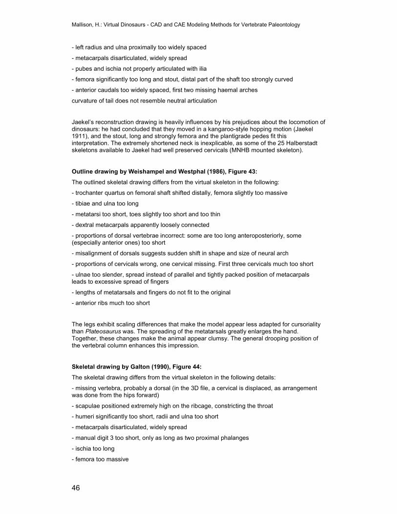
Mallison, H.: Virtual Dinosaurs - CAD and CAE Modeling Methods for Vertebrate Paleontology
46
- left radius and ulna proximally too widely spaced
- metacarpals disarticulated, widely spread
- pubes and ischia not properly articulated with ilia
- femora significantly too long and stout, distal part of the shaft too strongly curved
- anterior caudals too widely spaced, first two missing haemal arches
curvature of tail does not resemble neutral articulation
Jaekel’s reconstruction drawing is heavily influences by his prejudices about the locomotion of dinosaurs: he had concluded that they moved in a kangaroo-style hopping motion (Jaekel 1911), and the stout, long and strongly femora and the plantigrade pedes fit this interpretation. The extremely shortened neck is inexplicable, as some of the 25 Halberstadt skeletons available to Jaekel had well preserved cervicals (MNHB mounted skeleton).
Outline drawing by Weishampel and Westphal (1986), Figure 43:
The outlined skeletal drawing differs from the virtual skeleton in the following:
- trochanter quartus on femoral shaft shifted distally, femora slightly too massive
- tibiae and ulna too long
- metatarsi too short, toes slightly too short and too thin
- dextral metacarpals apparently loosely connected
- proportions of dorsal vertebrae incorrect: some are too long anteroposteriorly, some (especially anterior ones) too short
- misalignment of dorsals suggests sudden shift in shape and size of neural arch
- proportions of cervicals wrong, one cervical missing. First three cervicals much too short
- ulnae too slender, spread instead of parallel and tightly packed position of metacarpals leads to excessive spread of fingers
- lengths of metatarsals and fingers do not fit to the original
- anterior ribs much too short
The legs exhibit scaling differences that make the model appear less adapted for cursoriality than Plateosaurus was. The spreading of the metatarsals greatly enlarges the hand. Together, these changes make the animal appear clumsy. The general drooping position of the vertebral column enhances this impression.
Skeletal drawing by Galton (1990), Figure 44:
The skeletal drawing differs from the virtual skeleton in the following details:
- missing vertebra, probably a dorsal (in the 3D file, a cervical is displaced, as arrangement was done from the hips forward)
- scapulae positioned extremely high on the ribcage, constricting the throat
- humeri significantly too short, radii and ulna too short
- metacarpals disarticulated, widely spread
- manual digit 3 too short, only as long as two proximal phalanges
- ischia too long
- femora too massive
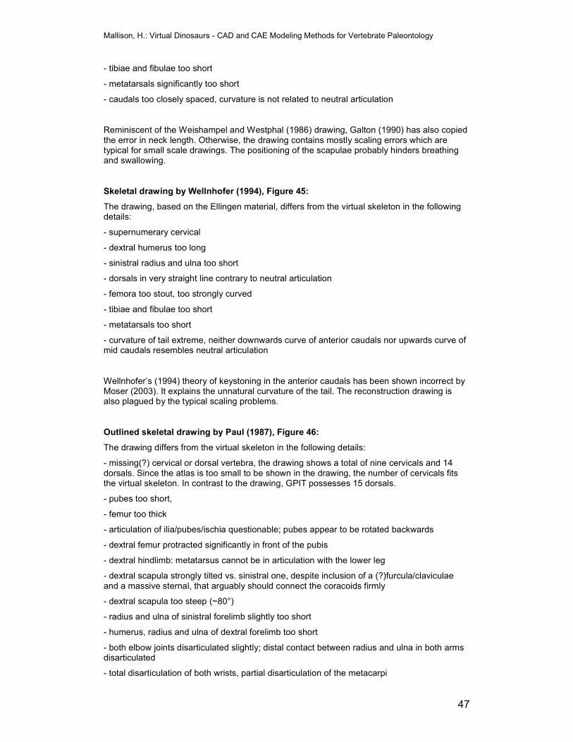
Mallison, H.: Virtual Dinosaurs - CAD and CAE Modeling Methods for Vertebrate Paleontology
47
- tibiae and fibulae too short
- metatarsals significantly too short
- caudals too closely spaced, curvature is not related to neutral articulation
Reminiscent of the Weishampel and Westphal (1986) drawing, Galton (1990) has also copied the error in neck length. Otherwise, the drawing contains mostly scaling errors which are typical for small scale drawings. The positioning of the scapulae probably hinders breathing and swallowing.
Skeletal drawing by Wellnhofer (1994), Figure 45:
The drawing, based on the Ellingen material, differs from the virtual skeleton in the following details:
- supernumerary cervical
- dextral humerus too long
- sinistral radius and ulna too short
- dorsals in very straight line contrary to neutral articulation
- femora too stout, too strongly curved
- tibiae and fibulae too short
- metatarsals too short
- curvature of tail extreme, neither downwards curve of anterior caudals nor upwards curve of mid caudals resembles neutral articulation
Wellnhofer’s (1994) theory of keystoning in the anterior caudals has been shown incorrect by Moser (2003). It explains the unnatural curvature of the tail. The reconstruction drawing is also plagued by the typical scaling problems.
Outlined skeletal drawing by Paul (1987), Figure 46:
The drawing differs from the virtual skeleton in the following details:
- missing(?) cervical or dorsal vertebra, the drawing shows a total of nine cervicals and 14 dorsals. Since the atlas is too small to be shown in the drawing, the number of cervicals fits the virtual skeleton. In contrast to the drawing, GPIT possesses 15 dorsals.
- pubes too short,
- femur too thick
- articulation of ilia/pubes/ischia questionable; pubes appear to be rotated backwards
- dextral femur protracted significantly in front of the pubis
- dextral hindlimb: metatarsus cannot be in articulation with the lower leg
- dextral scapula strongly tilted vs. sinistral one, despite inclusion of a (?)furcula/claviculae and a massive sternal, that arguably should connect the coracoids firmly
- dextral scapula too steep (~80°)
- radius and ulna of sinistral forelimb slightly too short
- humerus, radius and ulna of dextral forelimb too short
- both elbow joints disarticulated slightly; distal contact between radius and ulna in both arms disarticulated
- total disarticulation of both wrists, partial disarticulation of the metacarpi
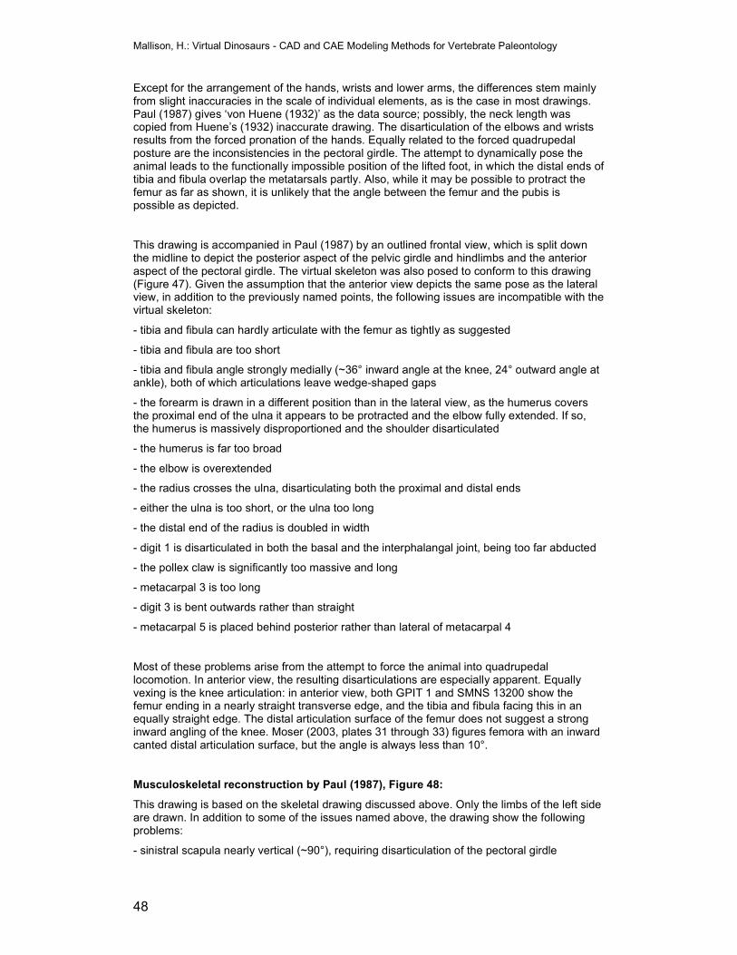
Mallison, H.: Virtual Dinosaurs - CAD and CAE Modeling Methods for Vertebrate Paleontology
48
Except for the arrangement of the hands, wrists and lower arms, the differences stem mainly from slight inaccuracies in the scale of individual elements, as is the case in most drawings. Paul (1987) gives ‘von Huene (1932)’ as the data source; possibly, the neck length was copied from Huene’s (1932) inaccurate drawing. The disarticulation of the elbows and wrists results from the forced pronation of the hands. Equally related to the forced quadrupedal posture are the inconsistencies in the pectoral girdle. The attempt to dynamically pose the animal leads to the functionally impossible position of the lifted foot, in which the distal ends of tibia and fibula overlap the metatarsals partly. Also, while it may be possible to protract the femur as far as shown, it is unlikely that the angle between the femur and the pubis is possible as depicted.
This drawing is accompanied in Paul (1987) by an outlined frontal view, which is split down the midline to depict the posterior aspect of the pelvic girdle and hindlimbs and the anterior aspect of the pectoral girdle. The virtual skeleton was also posed to conform to this drawing (Figure 47). Given the assumption that the anterior view depicts the same pose as the lateral view, in addition to the previously named points, the following issues are incompatible with the virtual skeleton:
- tibia and fibula can hardly articulate with the femur as tightly as suggested
- tibia and fibula are too short
- tibia and fibula angle strongly medially (~36° inward angle at the knee, 24° outward angle at ankle), both of which articulations leave wedge-shaped gaps
- the forearm is drawn in a different position than in the lateral view, as the humerus covers the proximal end of the ulna it appears to be protracted and the elbow fully extended. If so, the humerus is massively disproportioned and the shoulder disarticulated
- the humerus is far too broad
- the elbow is overextended
- the radius crosses the ulna, disarticulating both the proximal and distal ends
- either the ulna is too short, or the ulna too long
- the distal end of the radius is doubled in width
- digit 1 is disarticulated in both the basal and the interphalangal joint, being too far abducted
- the pollex claw is significantly too massive and long
- metacarpal 3 is too long
- digit 3 is bent outwards rather than straight
- metacarpal 5 is placed behind posterior rather than lateral of metacarpal 4
Most of these problems arise from the attempt to force the animal into quadrupedal locomotion. In anterior view, the resulting disarticulations are especially apparent. Equally vexing is the knee articulation: in anterior view, both GPIT 1 and SMNS 13200 show the femur ending in a nearly straight transverse edge, and the tibia and fibula facing this in an equally straight edge. The distal articulation surface of the femur does not suggest a strong inward angling of the knee. Moser (2003, plates 31 through 33) figures femora with an inward canted distal articulation surface, but the angle is always less than 10°.
Musculoskeletal reconstruction by Paul (1987), Figure 48:
This drawing is based on the skeletal drawing discussed above. Only the limbs of the left side are drawn. In addition to some of the issues named above, the drawing show the following problems:
- sinistral scapula nearly vertical (~90°), requiring disarticulation of the pectoral girdle
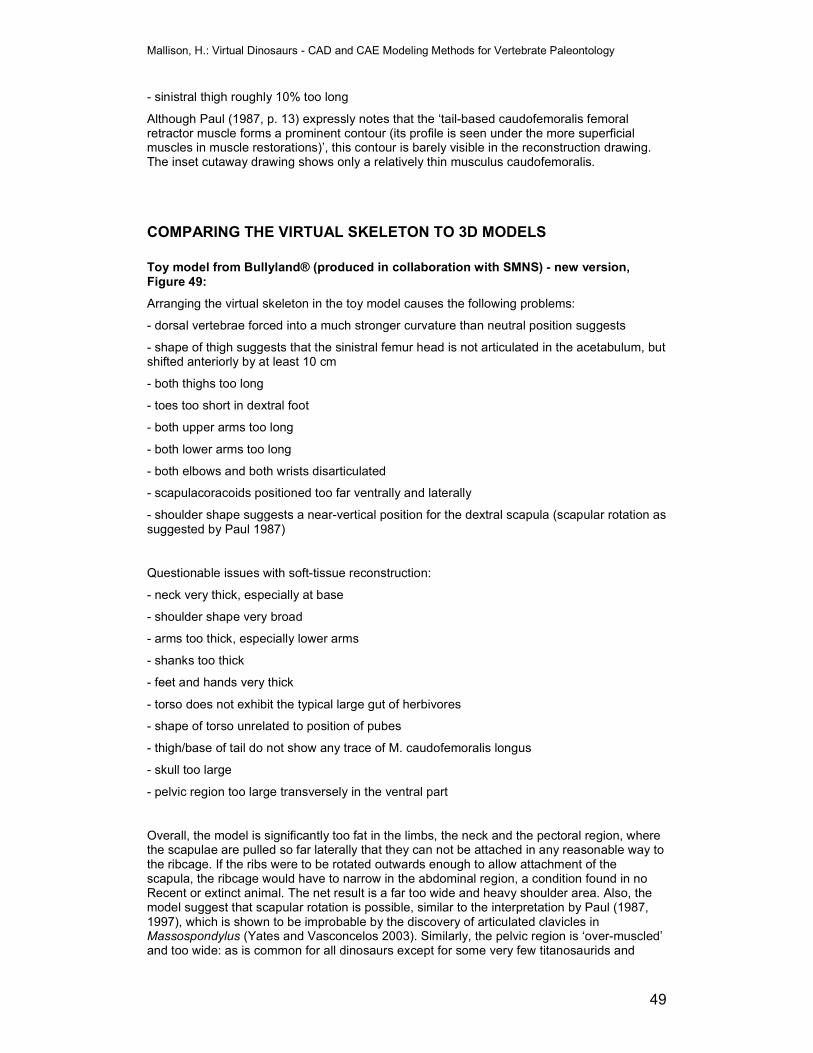
Mallison, H.: Virtual Dinosaurs - CAD and CAE Modeling Methods for Vertebrate Paleontology
49
- sinistral thigh roughly 10% too long
Although Paul (1987, p. 13) expressly notes that the ‘tail-based caudofemoralis femoral retractor muscle forms a prominent contour (its profile is seen under the more superficial muscles in muscle restorations)’, this contour is barely visible in the reconstruction drawing. The inset cutaway drawing shows only a relatively thin musculus caudofemoralis.
COMPARING THE VIRTUAL SKELETON TO 3D MODELS
Toy model from Bullyland® (produced in collaboration with SMNS) - new version, Figure 49:
Arranging the virtual skeleton in the toy model causes the following problems:
- dorsal vertebrae forced into a much stronger curvature than neutral position suggests
- shape of thigh suggests that the sinistral femur head is not articulated in the acetabulum, but shifted anteriorly by at least 10 cm
- both thighs too long
- toes too short in dextral foot
- both upper arms too long
- both lower arms too long
- both elbows and both wrists disarticulated
- scapulacoracoids positioned too far ventrally and laterally
- shoulder shape suggests a near-vertical position for the dextral scapula (scapular rotation as suggested by Paul 1987)
Questionable issues with soft-tissue reconstruction:
- neck very thick, especially at base
- shoulder shape very broad
- arms too thick, especially lower arms
- shanks too thick
- feet and hands very thick
- torso does not exhibit the typical large gut of herbivores
- shape of torso unrelated to position of pubes
- thigh/base of tail do not show any trace of M. caudofemoralis longus
- skull too large
- pelvic region too large transversely in the ventral part
Overall, the model is significantly too fat in the limbs, the neck and the pectoral region, where the scapulae are pulled so far laterally that they can not be attached in any reasonable way to the ribcage. If the ribs were to be rotated outwards enough to allow attachment of the scapula, the ribcage would have to narrow in the abdominal region, a condition found in no Recent or extinct animal. The net result is a far too wide and heavy shoulder area. Also, the model suggest that scapular rotation is possible, similar to the interpretation by Paul (1987, 1997), which is shown to be improbable by the discovery of articulated clavicles in Massospondylus (Yates and Vasconcelos 2003). Similarly, the pelvic region is ‘over-muscled’ and too wide: as is common for all dinosaurs except for some very few titanosaurids and
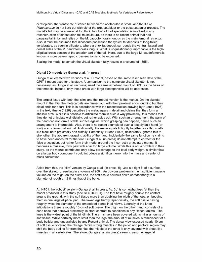
Mallison, H.: Virtual Dinosaurs - CAD and CAE Modeling Methods for Vertebrate Paleontology
50
ceratopians, the transverse distance between the acetabulae is small, and the ilia of Plateosaurus do not flare out with either the preacetabluar or the postacetabular process. The model’s tail may be somewhat too thick, too, but a lot of speculation is involved in any reconstruction of dinosaurian tail musculature, as there is no recent animal that has parasagittal limbs and relies on the M. caudofemoralis longus as the main femoral retractor. Also, it must be assumed that dinosaurs possessed the typical fat deposits of long-tailed vertebrates, as seen in alligators, where a thick fat deposit surrounds the ventral, lateral and dorsal sides of the M. caudofemoralis longus. What is unquestionably improbable is the high-elliptical cross-section of the anterior part of the tail. Here, due to the large M. caudofemoralis longus, a more pear-shaped cross-section is to be expected.
Scaling the model to contain the virtual skeleton fully results in a volume of 1355 l.
Digital 3D models by Gunga et al. (in press):
Gunga et al. created two versions of a 3D model, based on the same laser scan data of the GPIT 1 mount used for this study. A comparison to the complete virtual skeleton is not necessary, as Gunga et al. (in press) used the same excellent mount of GPIT as the basis of their models. Instead, only those areas with large discrepancies will be addresses.
The largest issue with both the ‘slim’ and the ‘robust’ version is the manus. On the skeletal mount in the IFG, the metacarpals are fanned out, with their proximal ends touching but their distal ends far apart. This is in accordance with the reconstruction drawing by Huene (1926). In the text, Huene (1926) describes the metacarpals in detail and claims that they form a shallow arch. While it is possible to articulate them in such a way proximally, this means that they do not articulate well distally, but rather splay out. With such an arrangement, the palm of the hand can not form a stable surface against which grasping can happen, hence such an arrangement is improbable. Also, there is no recent example of such a loosely built hand (or foot) in any terrestrial animal. Additionally, the metacarpals fit tightly together as a flat, shelf-like block both proximally and distally. Potentially, Huene (1926) deliberately ignored this to strengthen the apparent grasping ability of the hand, incidentally the same function he claims to have been ancestral for the foot! Gunga et al. (in press) do not attempt to correct for the false articulation, but rather form their model around the incorrectly articulated manus. It becomes a massive, thick paw with a far too large volume. While this is not a problem in their study, as the manus contributes only a low percentage to the total body weight, a similar flaw on a larger body component could introduce a significant error into the mass and center of mass calculation.
Aside from this, the ‘slim’ version by Gunga et al. (in press, fig. 3a) is a tight fit of a surface over the skeleton, resulting in a volume of 900 l. An obvious problem is the insufficient muscle volume on the thigh: on the distal end, the soft tissue narrows down unreasonably to a diameter of roughly 1.2 times that of the bone.
At 1470 l, the ‘robust’ version (Gunga et al. in press, fig. 3b) is somewhat less fat than the model produced in this study (see SECTION III). The feet have roughly double the contact area to the ground, with the soft tissue more than doubling the width of the toes, embedding them in one large elliptical pad. The lower legs hardly taper distally, the soft tissue having roughly twice the diameter of the embedded bones in all views. Laterally of the knee articulations there is roughly 10 cm of soft tissue. The thigh, on the other hand, consists of a cone base that narrows proximally, in stark contrast to conditions in any Recent animal. The knee is the widest point of the hindlimb. The arms have been covered with similar amounts of soft tissue. While certainly more stout than the legs, the amount of muscles is reminiscent of a body builder and unparalleled by any Recent animal. The dorsal view exposed nearly 10 cm of soft tissue covering the ribcage. While strong muscles in the pelvic and pectoral region may shift the body outline far from the ribs, the middle of the torso is only covered with sheet-like muscles in all vertebrates. Therefore, Gunga et al. (in press) seem to assume large fat
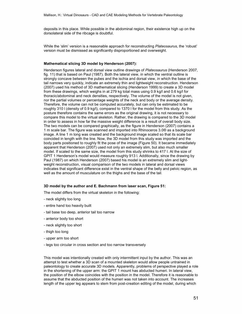
Mallison, H.: Virtual Dinosaurs - CAD and CAE Modeling Methods for Vertebrate Paleontology
51
deposits in this place. While possible in the abdominal region, their existence high up on the dorsolateral side of the ribcage is doubtful.
While the ‘slim’ version is a reasonable approach for reconstructing Plateosaurus, the ‘robust’ version must be dismissed as significantly disproportioned and overweight.
Mathematical slicing 3D model by Henderson (2007):
Henderson figures lateral and dorsal view outline drawings of Plateosaurus (Henderson 2007, fig. 11) that is based on Paul (1987). Both the lateral view, in which the ventral outline is strongly concave between the pubes and the ischia and dorsal view, in which the base of the tail narrows very quickly, indicate an extremely thin and lightweight reconstruction. Henderson (2007) used his method of 3D mathematical slicing (Henderson 1999) to create a 3D model from these drawings, which weighs in at 279 kg total mass using 0.9 kg/l and 0.6 kg/l for thoracic/abdominal and neck densities, respectively. The volume of the model is not given, nor the partial volumes or percentage weights of the neck and body or the average density. Therefore, the volume can not be computed accurately, but can only be estimated to be roughly 310 l (density of 0.9 kg/l), compared to 1370 l for the model from this study. As the posture therefore contains the same errors as the original drawing, it is not necessary to compare this model to the virtual skeleton. Rather, the drawing is compared to the 3D model in order to assess in how far the massive weight difference is a result of overall body size. The two models can be compared graphically, as the figure in Henderson (2007) contains a 1 m scale bar. The figure was scanned and imported into Rhinoceros 3.0® as a background image. A line 1 m long was created and the background image scaled so that its scale bar coincided in length with the line. Now, the 3D model from this study was imported and the body parts positioned to roughly fit the pose of the image (Figure 50). It became immediately apparent that Henderson (2007) used not only an extremely slim, but also much smaller model. If scaled to the same size, the model from this study shrinks to 417 l. At the size of GPIT 1 Henderson’s model would measure roughly 913 l. Additionally, since the drawing by Paul (1987) on which Henderson (2007) based his model is an extremely slim and light-weight reconstruction, visual comparison of the two models in lateral and dorsal views indicates that significant difference exist in the ventral shape of the belly and pelvic region, as well as the amount of musculature on the thighs and the base of the tail.
3D model by the author and E. Bachmann from laser scan, Figure 51:
The model differs from the virtual skeleton in the following:
- neck slightly too long
- entire hand too heavily built
- tail base too deep, anterior tail too narrow
- anterior body too short
- neck slightly too short
- thigh too long
- upper arm too short
- legs too circular in cross section and too narrow transversely
This model was intentionally created with only intermittent input by the author. This was an attempt to test whether a 3D scan of a mounted skeleton would allow people untrained in paleontology to create accurate 3D models. Apparently, problems of perspective played a role in the shortening of the upper arm: the GPIT 1 mount has abducted humeri. In lateral view, the position of the elbow coincides with the position in the model. Therefore it is reasonable to assume that the abducted position of the humeri was not taken into account. The increases length of the upper leg appears to stem from post-creation editing of the model, during which
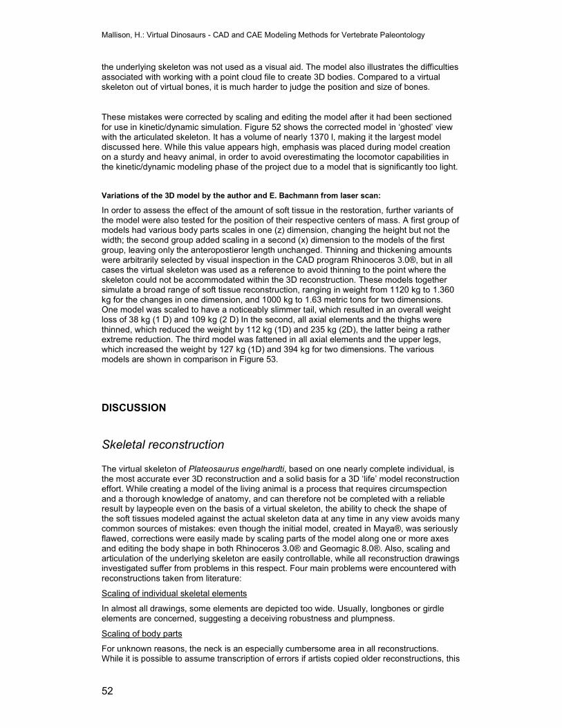
Mallison, H.: Virtual Dinosaurs - CAD and CAE Modeling Methods for Vertebrate Paleontology
52
the underlying skeleton was not used as a visual aid. The model also illustrates the difficulties associated with working with a point cloud file to create 3D bodies. Compared to a virtual skeleton out of virtual bones, it is much harder to judge the position and size of bones.
These mistakes were corrected by scaling and editing the model after it had been sectioned for use in kinetic/dynamic simulation. Figure 52 shows the corrected model in ‘ghosted’ view with the articulated skeleton. It has a volume of nearly 1370 l, making it the largest model discussed here. While this value appears high, emphasis was placed during model creation on a sturdy and heavy animal, in order to avoid overestimating the locomotor capabilities in the kinetic/dynamic modeling phase of the project due to a model that is significantly too light.
Variations of the 3D model by the author and E. Bachmann from laser scan:
In order to assess the effect of the amount of soft tissue in the restoration, further variants of the model were also tested for the position of their respective centers of mass. A first group of models had various body parts scales in one (z) dimension, changing the height but not the width; the second group added scaling in a second (x) dimension to the models of the first group, leaving only the anteropostieror length unchanged. Thinning and thickening amounts were arbitrarily selected by visual inspection in the CAD program Rhinoceros 3.0®, but in all cases the virtual skeleton was used as a reference to avoid thinning to the point where the skeleton could not be accommodated within the 3D reconstruction. These models together simulate a broad range of soft tissue reconstruction, ranging in weight from 1120 kg to 1.360 kg for the changes in one dimension, and 1000 kg to 1.63 metric tons for two dimensions. One model was scaled to have a noticeably slimmer tail, which resulted in an overall weight loss of 38 kg (1 D) and 109 kg (2 D) In the second, all axial elements and the thighs were thinned, which reduced the weight by 112 kg (1D) and 235 kg (2D), the latter being a rather extreme reduction. The third model was fattened in all axial elements and the upper legs, which increased the weight by 127 kg (1D) and 394 kg for two dimensions. The various models are shown in comparison in Figure 53.
DISCUSSION
Skeletal reconstruction
The virtual skeleton of Plateosaurus engelhardti, based on one nearly complete individual, is the most accurate ever 3D reconstruction and a solid basis for a 3D ‘life’ model reconstruction effort. While creating a model of the living animal is a process that requires circumspection and a thorough knowledge of anatomy, and can therefore not be completed with a reliable result by laypeople even on the basis of a virtual skeleton, the ability to check the shape of the soft tissues modeled against the actual skeleton data at any time in any view avoids many common sources of mistakes: even though the initial model, created in Maya®, was seriously flawed, corrections were easily made by scaling parts of the model along one or more axes and editing the body shape in both Rhinoceros 3.0® and Geomagic 8.0®. Also, scaling and articulation of the underlying skeleton are easily controllable, while all reconstruction drawings investigated suffer from problems in this respect. Four main problems were encountered with reconstructions taken from literature:
Scaling of individual skeletal elements
In almost all drawings, some elements are depicted too wide. Usually, longbones or girdle elements are concerned, suggesting a deceiving robustness and plumpness.
Scaling of body parts
For unknown reasons, the neck is an especially cumbersome area in all reconstructions. While it is possible to assume transcription of errors if artists copied older reconstructions, this
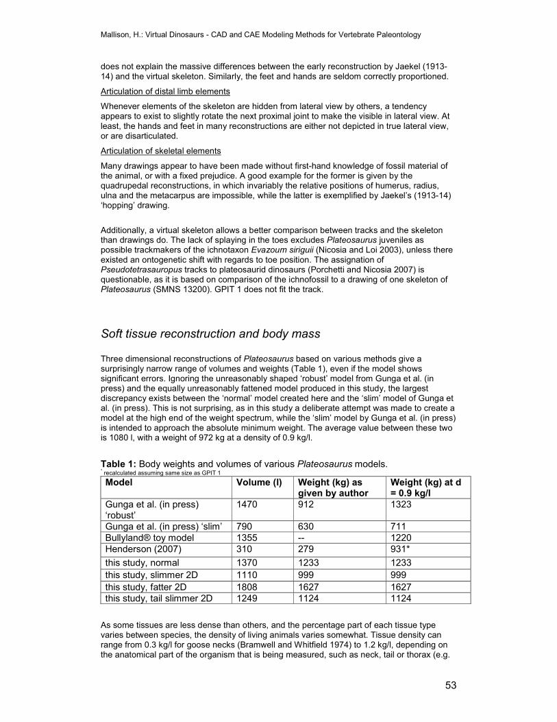
Mallison, H.: Virtual Dinosaurs - CAD and CAE Modeling Methods for Vertebrate Paleontology
53
does not explain the massive differences between the early reconstruction by Jaekel (1913-14) and the virtual skeleton. Similarly, the feet and hands are seldom correctly proportioned.
Articulation of distal limb elements
Whenever elements of the skeleton are hidden from lateral view by others, a tendency appears to exist to slightly rotate the next proximal joint to make the visible in lateral view. At least, the hands and feet in many reconstructions are either not depicted in true lateral view, or are disarticulated.
Articulation of skeletal elements
Many drawings appear to have been made without first-hand knowledge of fossil material of the animal, or with a fixed prejudice. A good example for the former is given by the quadrupedal reconstructions, in which invariably the relative positions of humerus, radius, ulna and the metacarpus are impossible, while the latter is exemplified by Jaekel’s (1913-14) ‘hopping’ drawing.
Additionally, a virtual skeleton allows a better comparison between tracks and the skeleton than drawings do. The lack of splaying in the toes excludes Plateosaurus juveniles as possible trackmakers of the ichnotaxon Evazoum siriguii (Nicosia and Loi 2003), unless there existed an ontogenetic shift with regards to toe position. The assignation of Pseudotetrasauropus tracks to plateosaurid dinosaurs (Porchetti and Nicosia 2007) is questionable, as it is based on comparison of the ichnofossil to a drawing of one skeleton of Plateosaurus (SMNS 13200). GPIT 1 does not fit the track.
Soft tissue reconstruction and body mass Three dimensional reconstructions of Plateosaurus based on various methods give a surprisingly narrow range of volumes and weights (Table 1), even if the model shows significant errors. Ignoring the unreasonably shaped ‘robust’ model from Gunga et al. (in press) and the equally unreasonably fattened model produced in this study, the largest discrepancy exists between the ‘normal’ model created here and the ‘slim’ model of Gunga et al. (in press). This is not surprising, as in this study a deliberate attempt was made to create a model at the high end of the weight spectrum, while the ‘slim’ model by Gunga et al. (in press) is intended to approach the absolute minimum weight. The average value between these two is 1080 l, with a weight of 972 kg at a density of 0.9 kg/l.
Table 1: Body weights and volumes of various Plateosaurus models. * recalculated assuming same size as GPIT 1
Model Volume (l) Weight (kg) as given by author
Weight (kg) at d = 0.9 kg/l
Gunga et al. (in press) ‘robust’
1470 912 1323
Gunga et al. (in press) ‘slim’ 790 630 711 Bullyland® toy model 1355 -- 1220 Henderson (2007) 310 279 931*
this study, normal 1370 1233 1233 this study, slimmer 2D 1110 999 999 this study, fatter 2D 1808 1627 1627 this study, tail slimmer 2D 1249 1124 1124
As some tissues are less dense than others, and the percentage part of each tissue type varies between species, the density of living animals varies somewhat. Tissue density can range from 0.3 kg/l for goose necks (Bramwell and Whitfield 1974) to 1.2 kg/l, depending on the anatomical part of the organism that is being measured, such as neck, tail or thorax (e.g.
Mallison, H.: Virtual Dinosaurs - CAD and CAE Modeling Methods for Vertebrate Paleontology
54
Anderson et al. 1985, Christiansen and Farina 2004, Colbert 1962, Gunga et al. 1999, Henderson 1999, 2007, Lambert 1980, Motani 2001, Schmidt-Nielsen 1984, 1997, Seebacher 2001, Wedel 2003b, 2005). Generally, terrestrial animals have an overall density of roughly 1 kg/l, but values as high as 1.15 kg/l (Bellmann et al. 2005) have been measured. Some researchers assume that the extensive air sac system of sauropods reduced their density significantly, with the trunk density at 0.8 kg/l and a neck density of 0.3 kg/l (Henderson 2007). For prosauropods, it is unclear whether they had an air sac system reminiscent of birds, or a more crocodile-like lung system. Gunga et al. (in press) and Henderson (2007) assume a trunk density of 0.9 kg/l and a neck density of 0.6 kg/l. As there is no clear evidence for pneumaticity in prosauropods, it is still likely that they possessed air sac systems (Wedel 2007). For the sake of simplicity, the neck in this study was set to the same density as the rest of the body, 0.9 kg/l. If this value is wrong, then it makes the animal more front-heavy than it should be, ensuring that wrong density values to not make a bipedal pose seem possible that in reality is not balanced. On this basis it seems reasonable to assume that Plateosaurus weighted about one ton at the size of the GPIT 1 individual.
For Brachiosaurus brancai, a volume of 46 m3 was determined. Densities were assigned following Henderson (2007), with the neck set to 0.3 kg/l, the thoracic/abdominal density assumed to be 900 kg/l and the tail and limbs set to 1 kg/l. This resulted in an overall weight of 37.515 tons, compared to 25.992 tons in Henderson (2007). As with Plateosaurus, this discrepancy is not surprising, as a heavy model was preferred for later use in kinetic/dynamic modeling. As Brachiosaurus is not the main subject of this study, the various other mass estimates in the literature will not be discussed here. The model serves simply as further indication that 3D reconstructions offer a valid tool for mass estimates if applied properly.
CONCLUSIONS SECTION II
Virtual skeletons constructed from digitized bones prove an easily applicable and useful tool for paleontologists attempting to reconstruct the body volume of an extinct vertebrate. 3D model creation in a CAD software on the basis of a virtual skeleton is easy and does not run the risks of incorporating mistakes from other sources or work processes, as models based on reconstruction drawings often do. While the method is inherently slightly more accurate than the 3D mathematical slicing described by Henderson (1999), due to the fact that more and usually more accurate data is used, both methods are quite similar, and the differences between them become negligible if the mathematical slicing method is used with sufficient and accurate input data. Compared to the method of Gunga et al. (in press), using a virtual skeleton allows basing the model on a correctly articulated skeleton, while using a laser scan of a mount risks inheriting the mount’s flaws. While it is possible to edit scan data, this is at best a difficult process, since the surfaces are not well visualized.
The biggest advantage of the virtual skeleton method described here is the ability to check the articulation of bones and the position of the skeletal elements within the 3D model at any time from any angle. Still, the results of the volumetric estimates are within the same general range. Additionally, using a CAD program allows easy scaling, to produce a series of slightly different models with varying amounts of soft tissues.
Classic skeletal drawings were found to often contain typical errors, mostly with regards to the scaling of bones. Due to the small size of a drawing compared to the real bones, the thickness of bones is often exaggerated. Digits, but sometimes also the metacarpus and metatarsus, are often given incorrect lengths, and some authors tend to twist those elements into view that are hidden by others, which may place them into disarticulated positions. These and other common errors make skeletal drawings critically inaccurate: often, they suggest proportions and therefore locomotion capabilities that are not correct.
Mallison, H.: Virtual Dinosaurs - CAD and CAE Modeling Methods for Vertebrate Paleontology
55
The skeletal morphology of Plateosaurus unambiguously indicates obligate bipedality and digitigrady. The morphology of the basal phalangal articulation and the shape of the metatarsus show that the metatarsus was held near vertical during times of high stress. The proximal phalanges were also held in a steep position, and the animal walked mostly on the distal phalanges. Except for the splaying of the toes in Evazoum siriguii, this track is similar in overall morphology, albeit much smaller. The ichnofossils Tetrasauropus can not stem from Plateosaurus, as it is a quadrupedal trackway. Pseudotetrasauropus, also classically assigned to plateosaurid dinosaurs and their close relatives, can not be brought into accordance with the foot of GPIT 1, but is quite similar to SMNS 13200.
The living weight of Plateosaurus is determined to be around to slightly over one metric ton by several studies, which agrees with the results presented here. While Henderson (2007) determines a significantly smaller mass, this is due to his use of a much smaller overall animal; scaled up his model also reaches the same weight range.
Mallison, H.: Virtual Dinosaurs - CAD and CAE Modeling Methods for Vertebrate Paleontology
56
SECTION III
INTRODUCTION TO SECTION III
How animals move, especially their gaits, speeds and their endurance during locomotion, but also other motions such as e.g. burrowing, has interested mankind for as long as there was intensive interaction between man and animal. Arguably, the first to study animal (loco-)motion were stone-age hunters, who also created the beautiful drawings of animals in the caves of Lascaux, Altamira, Rouffignac, Chauvet and many other places worldwide, paintings and drawings of astonishing accuracy. Not only are the animals depicted with correct proportions, making them easily recognizable, but often also in subtle exaggeration of their natural postures during locomotion. Aristotle was the first to write a book (Aristotle unknown) on biomechanical questions. From Roman times and all through the Middle Ages, especially those animals important for military and agricultural purposes became the center of attention. Horses were studied at great length, although not necessarily for scientific interest and with scientific standards.
Locomotion studies took a marked upturn with the famous work of Muybridge (1887), who used a setup of photographic cameras, their shutters controlled with tripwires, creating sequences of still pictures at regular intervals to show that each hoof of a galloping horse hits the ground just as another is leaving it, so that a horse at full gallop is deriving traction from only one hoof at a time.
As biomechanical studies of locomotion and related energy expenditure have been a center of research for decades, this section can only give a very selective overview of some important issues.
Many researchers have tried to understand the locomotion of animals by the use of simplified physical models, in which motions are represented by levers and forces acting on them (e.g. Alexander 1976, Kummer 2005, Kuznetsov 1995). These helpful approaches are limited by the need to simplify the models greatly, in order to keep them at a manageable complexity. Limbs are represented by one-piece rods in the simplest models. Alexander (1976, 1977) and Alexander and Vernon (1975) developed a standardized model for the typical reptilian two-segment limbs and the typical mammalian three-segment limbs, and some researchers have specifically addressed the problem of the complex motions possible in multi-part limbs and the resulting energy savings (e.g. Kuznetsov 1995).
Elastic properties of muscles and tendons play an important role in preserving energy, as shown e.g. by the work of Dawson and Taylor (1973).
All these approaches suffer from one basic problem, though: mass is usually regarded as a point object at the location of the center of gravity, and inertia, especially rotational inertia, is much simplified or missing from the calculations (Alexander 1976, 1977, Kuznetsov 1995). The complex shift in length of a limb during the swing forward, for example, constantly alters the position of the center of mass and the deviation of its path relative to the hip joint compared to a simple pendulum swing. Rotational inertia is transferred from one segment to its neighboring segments whenever muscles act on them, a factor that must be ignored in simple models. Vertical or lateral motions of the trunk are equally ignored. Also, the reaction force created by the ground against the foot is usually simplified, e.g. by assuming that at the moment of maximum reaction force the hip is placed directly above the contact point between foot and ground (Blanco 2003). Elastic properties of tendons and muscles are often considered or measured in a simplified form, especially considering the interesting phenomenon of the locomotion of Macropodidae (e.g. Alexander and Vernon 1975, Blanco and Gambini 2006, Cavagna et al. 1977) , who at high speeds keep a stable metabolic rate, opposed to the increasing rate in most other animals (see e.g. Taylor et al. 1982). Basically,
Mallison, H.: Virtual Dinosaurs - CAD and CAE Modeling Methods for Vertebrate Paleontology
57
most models used are kinematic, describing the geometry of motions without the influence of masses and their inertia. Rudimentary addition of mass allows simple kinetic models, such as the one by Farlow et al. (1995), who calculated the forces on the body and skull of Tyrannosaurus rex resulting from a fall, but they are far from being able to exactly describe the motion capabilities of animals in detail. While Farlow et al. (1995) do allow for a skid distance after stumbling, they do not allow for a rolling motion of the animal, or for internal motions that could cushion an impact. Also, it is not reasonable to assume that animals will not risk falling. A better approach was taken by Blanco and Mazzetta (2001), who instead calculated the speed at which recovery is still possible, arriving at far higher maximum speed estimates.
Many approaches use extrapolation from smaller animals to make predictions about extinct taxa. Usually, a regression line is at the heart of the extrapolation, which always involves a large uncertainty when large size differences exist between the Recent taxa the regression is calculated from and the extinct taxa to which the regression is extended (e.g. Hutchinson and Garcia 2002). This fact is often hidden by the logarithmic scale of the diagram axes, but error bars of +/- 50 percent are common. Henderson (2007, p. 910) notes that ‘[i]t is poor practice to extrapolate an allometric relationship beyond the original range of data used to define it’. Also, the sampled Recent taxa must be chosen carefully: any mass estimate of large terrestrial animals based on longbone strength can for example be seriously hurt by the inclusion of the semi-aquatic hippopotamus. Locomotory predictions depend on accurate collection of large amounts of data and their correct interpretation.
Other approaches describe locomotion as a series of static poses, instead of a dynamic process. This is e.g. the case for Henderson (2007), who modeled sauropod locomotion for very slow gaits by assuming a stability criterion based on a static analysis: the center of gravity had to rest within a triangle of support points on the ground. Basically, Henderson (2007) took ‘snapshots’ of the modeled locomotion and treated each as a static pose. This limits the animal to gaits with alternating three-point and four-point support stages, termed ‘very slow diagonal walk’ by Sukhanov (1967). Gambaryan (1974) notes that with a duty factor (which he terms ‘rhythm of limb work’) of 0.75, in quadrupeds the four-point support stages disappear. At any lower value, Henderson’s criterion of three-point support (Henderson 2007) will not be fulfilled at some stage of the walking cycle. In analogy to Henderson (2007), a human would never be able to walk normally, as forward motion of the body could only happen while both feet are on the ground. Obviously, this is not true: we walk with a nearly constant body velocity, and inertia keeps the body from falling a significant distance before the leg being protracted is in a sufficiently forward position to catch the ‘fall’. The same is also true for quadrupeds, even extremely heavy ones like elephants: screenshots from a video taken at the Tierpark Berlin show clearly that quickly walking elephants have at most three feet on the ground, but often are supported by only two (Figure 54, Video: Loxodonta fast walk.avi). Hutchinson et al. (2003) shows that this support can even be reduced to one limb on the ground, which is then near the vertical position. This has also been described by Gambaryan (1974), who noted that the elephant’s ‘fast walk’ includes one-point support phases regularly. A scheme of outline drawings detailing this ‘fast walk’ is given in Gambaryan (1974, fig. 113). Obviously, while the approach is certainly useful to study gaits that produce known fossil trackways, which were usually made when the animals walked slowly on slippery ground (Mazzetta and Blanco 2001), Henderson’s (2007) approach unduly limits sauropod locomotion when a full assessment of their locomotor capabilities is desired.
Kinetic/dynamic modeling, as opposed to kinematic modeling, does not only deal with and describe the motions of objects, but includes their masses and inertia into the calculations (Kummer 2005). While a kinematic model may be adequate to describe the geometry of possible motions, it does not answer the question whether the motion is realistic. An excellent example would be a kinematic model of the human leg, which shows that for locomotion, it is possible to swing the leg forward during the recovery stroke in a sideways motion: lifting the foot laterally by abducting the thigh. Though possible, this motion does not make sense biomechanically, as an inordinate amount of rotational inertia is produced which has to be
Mallison, H.: Virtual Dinosaurs - CAD and CAE Modeling Methods for Vertebrate Paleontology
58
compensated for in order to keep the leg from continuing to swing once the foot is in front of the body and crossing over the other leg – resulting in the other foot catching the leg, a sure way to stumble and fall. A kinetic model, on the other hand, does show the transfer of rotational inertia, and allows the research to distinguish those motions that are sensible from a functional morphology and biomechanics point of view from those that are not.
AIMS
In the last part of the project, the previously created 3D models of Plateosaurus were to be used as test object for kinetic/dynamic modeling in a NASTRAN based modeling software for desktop PCs. The first task was to determine whether NASTRAN can be employed in biomechanical paleontological research, especially with regards to questions of posture, balance and locomotion. The software of choice is MSC.visualNastran 4D®, and standardized methods for creating, controlling and evaluating simulation models for vertebrate paleontology had to be developed, since the program documentation only gives a generalized description of program components, not on their possible uses for various tasks. Of great concern was designing methods that allow checking simulation results against outside data to judge their probability. Ideally, these methods should be simple enough to allow rapid comparison of closely related and therefore proportionally similar taxa by scaling of components.
BASICS OF LOCOMOTION RESEARCH
With regards to locomotion, the most extensively studied animal is man himself, due to the needs of medical treatment. Both healthy and abnormal locomotion patterns have been studied extensively, since disabilities and illnesses that hinder locomotion can greatly decrease the ability to function in society. Conveniently for this study, Homo sapiens is an obligate biped, as is Plateosaurus. This allows adapting some important terminology based on the medical literature; especially on Whittle (1996). Especially important is the terminology of major events during a walking cycle given in Whittle (1996), on which the description used here is based. As shown in Figure 55, Whittle sections a walking cycle for normal human walking into seven phases, separated by eight distinct positions of the limbs. While some of these such as ‘Heel rise’ can not be applied to digitigrade animals like Plateosaurus, the principal points can be used easily. Here, the following succession is used: a cycle starts with the initial contact of the right foot with the ground (termed ‘Initial contact’ in Whittle (1996) and ‘heel strike’ in other publications on human locomotion), continues to ‘Opposite toe off’, then ‘ankles adjacent’ (replacing ‘Heel rise’ in Whittle 1996) and ‘Opposite initial contact’, concluding the ‘Stance phase’. Now, the ‘Swing phase’ follows, which is a mirror image of the opposite foot’s motion between ‘Opposite toe off’ and ‘Opposite initial contact’ and only divided by ‘Ankles adjacent’ (Figure 55). This scheme is somewhat simpler than those usually used for human locomotion. In this study, all walking cycles were limited to duty factors (percentage of a cycle that a foot is in contact with the ground) of more than 0.5. This precludes the use of unsupported (‘flight’) phases, which would further complicate the ground reaction force problems known to exist in MSC.visualNastran 4D®.
Aside from moving from one place to another, which is the purpose of locomotion, its most important aspect is the expenditure of energy. As soon as an animal lifts itself from a resting pose on the ground, it spends energy. Animals with parasagittal limbs spend a not negligible amount of energy just standing still, and much more energy is spent moving around. Obviously, under normal circumstances the main objective for locomotion is to move from one place to another in a way that minimizes the energy spent. Normally, faster locomotion means more energy spent. If the total time spent for traveling a given distance becomes an issue, e.g. during migration or flight, energy and time can be traded for each other. In quadrupedal animals, a wide variety of cyclic limb motions termed ‘gaits’ allow optimization of this speed/energy problem, so that the energy spent per distance can remain nearly constant. This is seen e.g. in horses, which use approximately the same amount of energy per distance
Mallison, H.: Virtual Dinosaurs - CAD and CAE Modeling Methods for Vertebrate Paleontology
59
when walking, trotting or galloping at the respective ideal speed of each gait (Hildebrand and Goslow 2003a). This involves the inclusion of additional joints in locomotion (e.g. bending and extension of the back) and extensive use of energy-conserving mechanisms, e.g. the use of muscles and tendons as elastic springs (Hildebrand and Goslow 2003b). Bipeds are more limited: in principle, they have only two gaits: a symmetrical right leg - left leg cycle called walking at low speeds and running if it incorporates unsupported phases at high speeds, and hopping, which is asymmetrical. For large animals, hopping requires special adaptations, as seen in the macropodidae. All other Recent large bipeds such as large running birds and humans normally use walking/running almost exclusively.
An important aspect of locomotion is the preservation and transfer of energy. Ideally, all energy spent when locomoting is spent moving the animal forward. In reality, much energy must be wasted on keeping the animal ‘on track’: to counter rotational inertia, for example, which is produced because there necessarily is a lever arm in the transverse axis between the center of mass and the attachment point of the limb, also to lift the body with each step because of a fixed limb length (principle of the standing pendulum, see e.g. Ahlborn 2004, Kummer 2005), or to counter torques in bent joints if the limb length is adjusted to keep the center of mass on a horizontal track. Obviously, the last two points are the extremes of a gradual trade-off, and optimizing this process is an important part of keeping the energy expenditure for locomotion minimal while optimizing speed. Additionally, the transfer of one type of energy into another is important: kinetic energy can be stored in muscles and tendons or transferred into potential energy by lifting the body and released at appropriate times - provided the motion is in correct phase with the frequencies of the storing material. An extensive introduction to this topic can be found in Hildebrand and Goslow (2003a, 2003b).
INTRODUCTION TO THE MODELING SOFTWARE
Here, only a short description of the modeling software and its main elements is given. This description consists of a summary of the program documentation for those parts relevant for this project, plus some explanations and comments on their use in this study. The next chapter then addresses the methods developed in this project for creating and modifying a simulation model of a terrestrial vertebrate for biomechanical analysis.
NASTRAN is a general purpose finite element analysis (FEA) program, originally produced by NASA and mainly written in FORTRAN. NASTRAN addresses a wide range of engineering problem-solving requirements (e.g. beam versus plate structures and various types of response such as statics or dynamics) as compared to other, more specialized programs, which concentrate on particular types of analysis. Figure 56 shows a screenshot of the work environment, in which the important features are indicated.
MSC.visualNastran 4D is a commercially available software package based on NASTRAN that allows finite element analysis (FEA) and kinetic/dynamic modeling for 3D body assemblages. As with all NASTRAN versions, the program handles rigid bodies exclusively. Rigid bodies do not deform or break apart during simulation, even though a physical object (the subject of simulation) may actually do so. In order to simulate flexible bodies—such as a bending beam — it is necessary to connect a series of rigid bodies with appropriate constraints to approximate the flexible body.
MSC.visualNastran 4D® solves problems using a variety of sophisticated numerical methods. Problems are time-discretized so that MSC.visualNastran Desktop 4D® computes motion and forces, while making sure that all the constraints are satisfied. With its systematic approach, MSC.visualNastran Desktop can model a wide variety of problems using numerical integration. Both the fast and simple Euler integration with fixed integration intervals and the more accurate Kutta-Merson integration that allows variable time steps are available in
Mallison, H.: Virtual Dinosaurs - CAD and CAE Modeling Methods for Vertebrate Paleontology
60
MSC.visualNastran 4D®, but only the latter was used in this study. Kutta-Merson integration is described in detail in Fox (1962). It requires significantly more computing power than the Euler integration.
For further information on the modeling see the MSC.visualNastran 4D® help files, chapter ‘Technical information’.
Model components and properties Note: in order to avoid confusion, program components of MSC.visualNastran 4D® are referred to in squared brackets, as in the program. Thus, ‘[body]’ refers to a 3D object imported into the simulation, while ‘body’ refers to the torso of the animal modeled.
A model in MSC.visualNastran 4D® consists of a set ob 3D objects or bodies, referred to in the program as [body]s. These can be imported into MSC.visualNastran 4D® from any CAD program. In this study, only stereolithography files (*.STL) were used as transfer formats. Aside from the visual appearance in the program, a body can be assigned values for a large number of physical properties. Here, only those are described that were either used, or could potentially influence locomotion analyses but were not changed from the default settings:
- central inertia: ‘uniform’, the default value, was selected in all models for all bodies
- CM (position of the center of mass): here, an offset for the cm can be entered; mass distribution is then calculated along with the changes in central inertia by the program. No use was made of this feature in this study.
- contact: here, the user can define how the program handles collisions between bodies. The default model is based on an impulse/momentum model, for which the user can define the coefficient of friction and of restitution (what percentage of collision energy is returned to the bodies after collision, i.e. how elastic is the collision?) Alternatively, the user can define freely both the normal force and the friction force with any formula.
- keyframe: a body can be assigned a certain position (x,y,z values plus rotation around x,y and z axes: rx, ry, rz) for any timestep. This position assignment supersedes any physics-based calculation and was not used in this study.
- material: here, material properties can be assigned. MSC.visualNastran 4D offers a wide range of presets for materials that are used in industrial applications. The following values can be set: density, elastic modulus, Poisson’s ratio, yield stress, ultimate tensile stress, specific heat, thermal conductivity and the thermal coefficient of expansion. Only the density was adjusted in this study.
- world position: the relative position of the body can be defined in x,y,z and rx, ry and rz.
Each [body] has a specific coordinate system. The relative position of this coordinate system versus the general ‘world’ coordinate system of the program is defined by the position of the [body] in the CAD program.
[body]s can be connected to one another with [constraint]s, and [meter]s can be attached to their center of mass. [input]s can be defined for various values such as position, speed, etc. In order to define where exactly a [constraint] or [meter] is to attach to the [body], a [coordinate] must be placed on the [body]. A [coordinate] is positioned via values for the position on the object (x, y, z) and its rotation versus the object coordinate system (rx, ry, rz), or by the same values in the ‘world’ coordinate system.
[constraint]s are connections between two [coordinate]s that follow certain rules. One [coordinate] on one of the two [body]s is the ‘base’ [coordinate], defining the axes of the
Mallison, H.: Virtual Dinosaurs - CAD and CAE Modeling Methods for Vertebrate Paleontology
61
[constraint]; the other [coordinate] on the other [body] may be aligned to the ‘base’ by the program at the creation of the [constraint]. This is necessary if the [constraint] limits rotation or shift around or along axes; if only the distance between the [coordinate]s is limited (‘rope’, ‘rod’ and ‘separator’ [constraint]s), the two [coordinate]s are not aligned. The user can specify rules concerning the force/torque, position, acceleration or velocity for the x, y, z or rx, ry and rz coordinates of the two coordinates between which the constraint is established. For these rules, the equations =, >= and <= are available. A large number of constraint types are available as presets, e.g. rotary joint, rigid joint, rope or linear actuator. [constraint] types are explained in more detail below, where the use of specific types in locomotion research models is also described.
[force]s can be applied at any desired point via a [coordinate]. The direction is controlled by defining force values for each axis. The applied force for each axis itself can be controlled by a formula. Scant use was made of this feature in the study presented here.
An [input] allows the user to enter numerical data into MSC.visualNastran 4D. [input] types are:
- slider: an interactive input which the user can move while the simulation is running; maximum and minimum values and the number of steps between them can be predetermined.
- table: a table in which the user can define timesteps and the input variable at each timestep. Tables can only be edited if the simulation is stopped and set to t = 0 s. If the simulation is not returned to the starting point, MSC.visualNastran 4D® will automatically reset it and delete the motion history when a table is edited. MSC.visualNastran 4D offers four modes of calculating data between timesteps: piecewise constant, piecewise linear, quadratic spline and cubic spline.
Formulae:
In addition to sliders and tables, for many features in MSC.visualNastran 4D the user can specify mathematical formulae as input. For example, the orientation of a revolute motor can be defined as a function of time, e.g. rx(t)=3*sin(t)+90° (the rotation of this joint around the x-axis will be equal to three times the sinus of the time value plus 90 degrees), or as the function of a property of another element of the simulation, e.g. rx(t)=[body3].r.y (the rotation of this joint around the x-axis will be equal to the rotation of [body3] vs. the world coordinate system around the y-axis). There is no practical limit to the complexity of the functions, except for a 255 character limit in the formula. MSC.visualNastran 4D® allows a large number of fields for each type of identifier to be used in these formulae. For bodies these include: position, rotation, velocity, angular velocity, acceleration, angular acceleration, momentum, angular momentum, kinetic energy, potential energy and the position of the center of mass. For constraints the position, orientation, acceleration, torque, force or tension can be defined.
During the simulation, many values can be measured in [meter]s. A [meter] is attached either directly to a [body] or [constraint], in which case it refers to the center of gravity of the [body] or attaches itself to the ‘base’ coordinate of the [constraint]. [meter] data is displayed in a separate window, either as a digital value for each measured parameter, or as a graph. [meter]s can be extensively customized, and their data can also be exported as Microsoft EXCEL® tables or a *.txt file.
Simulation results For each simulation, a, a full simulation report in *.htm format can be exported. It includes data on document properties, file size, input settings (analysis type, tolerance, integration,
Mallison, H.: Virtual Dinosaurs - CAD and CAE Modeling Methods for Vertebrate Paleontology
62
gravity, unit settings), model details (assembly table including masses and volumes, [constraints] table, material properties table, boundary conditions, initial conditions and FEA details [if FEA is chosen]). [meter]s and videos of the main simulation window can be added at will, along with external related files. This file contains all data related to the simulation file. [meter]s. The results of the simulation are displayed in program for each animation step (which corresponds to one or more integration steps, depending on the settings chosen) in the main simulation window. This display can be exported as a video file in various formats. [meter]s can be incorporated in these video files, but this option is limited to a single [meter] per video. [meter] data can also be exported as either Microsoft EXCEL® tables or as simple text files (*.txt).
Model creation In principle, creating a model is effected by importing the [body] objects, setting their properties, placing [coordinates] on them, connecting these with the desired [constraint] types, and creating and customizing all [meter] objects and data input for the simulation run, such as tables and formulae of all [input] types. Certain issues need to be kept in mind when planning and building a model:
1) MSC.visualNastran 4D® regards [body]s connected by ‘rigid’ constraints as one object. Also, any degree of freedom that is set fixed (e.g., sliding along x, y and z axes and rotation around x and z axes in a y-axis rotary joint) are regarded as ‘rigid’ connections. MSC.visualNastran 4D® also does not calculate several connection points between two objects. Therefore, if two [constraint]s with the same degree of freedom and coinciding axes are used to connect two [body]s (e.g. the two hinges of a door), one will be ignored by the program as redundant. Redundant constraints are problematic in so far as bearing loads are not distributed properly if there is more than one [constraint] on the same axis. If, e.g., a model of a bipedal animal is created with all limb joints set as rotary motor [constraint]s with rotation around the transverse axis as the only degree of freedom, the model will be overdefined if all [constraint]s are defined with regard to their orientation.
A simple solution to this problem is always leaving one [constraint] in a ‘closed-loop’ system ‘open’ - e.g. by setting a torque instead of an orientation as input. Alternatively, one or several [constraint]s can be set to ‘bushing’ type. They are then modeled as a combined spring/damper system for all six degrees of freedom. It is difficult and time consuming to set proper values, and the simulation will run very slow due to the added calculation effort. Hence, this solution was not used in this project.
2) MSC.visualNastran 4D® is a rigid body simulation. Therefore, [body]s do not deform upon collision, their contacts are always elastic collisions. In order to simulate inelastic collisions with the in-built collision mode (impulse/momentum model), the coefficient of restitution can be set for each object. The [body]s still will not show change in shape, but the energy loss is represented. This creates two problems:
The first problem, incorrect motion, is best explained by an example: imagine a bowling ball with a pencil stuck in one hole. If the assemblage is dropped ball-first on a clay floor, it will slightly deform the clay and come to rest on top of it. If, on the other hand, the assemblage is dropped pencil-first, the ball will ram the pencil into the clay, and the assemblage comes to rest only when the ball collides with the ground. In MSC.visualNastran 4D®, on the other hand, the model will behave differently: dropped ball first, it will mimic the real world minus the deformation of the ground, but dropped pencil-first, it will bounce on the tip of the pencil!
Second, while working well for small masses, the forces applied to one object by another become very large for large masses or high velocities, either due to deep penetration (high speed) at collision or high momentum (large masses). In order to solve the motion correctly, the time step is reduced during integration by the software. This is problematic, as at any
Mallison, H.: Virtual Dinosaurs - CAD and CAE Modeling Methods for Vertebrate Paleontology
63
given tolerance, the two bodies will not be in contact at one time step, but be in contact in the next. Therefore, decreasing the integration time step will reduce the penetration, but the momentum changes remain, since there is now less time available. Again, the time step is reduced, until at some point the model leaves the accuracy limit: the resulting force will be rounded with an error that becomes significant compared to the time step. For example, a heavy body colliding with a bigger, inert one under the influence of gravity may be erroneously assigned a return velocity bigger than 0 m/s, even if the coefficient of restitution is set to 0. Therefore, for an extremely short time interval, the object will bounce back, then fall back on the other object, then bounce back again, etc. A typical problem resulting from this is a miniature version of ‘chattering’, a rapid bouncing effect encountered in walking robots. As a direct result, the object will not experience any friction, leading to an ‘ice skating’ effect: it appears to slide, while in reality it is bouncing up and down a very small distance at a very high frequency. This effect is not visible, since the animation time step is much lower. There is no trivial solution to this problem within the scope of this project, as any integrative solver of a rigid body system will always face this problem.
These two problems can be ameliorated by choosing custom formulae for the normal and friction forces. The author has tested various approaches, but none of them resulted in satisfactory results across the wide range of masses and velocities involved in this project. Especially problematic are contacts in which one object rotates. Since the normal force is applied to the center of mass, the rotation may increase, and the motion may result in an inadequate reaction force. Theoretically, it should be possible to make the normal force dependant not on the penetration depth, but on the penetration volume. This would allow scaling the reaction force properly, but the complicated mathematics involved are beyond the scope of this project. As an easier and faster alternative to adapting the normal forces model, workarounds were found. One option is to simply connect a body to the ground with a joint type that allows all necessary motions. This [constraint] can be set to become active only at certain times, e.g. a foot can be disconnected from the ground until the moment it touches the ground. While not free of problems, such as MSC.visualNastran 4D® attempting to ‘force’ the [constraint] and exerting huge forces on the two [body]s that are to be connected, this is sufficient for simpler models. Alternatively, the impacting body can be slowed down by adding a ‘ghost’ ground just above the ‘real’ ground, and giving this second ground object collision properties sufficient to slow the collision with the ‘real’ ground to speeds and momentums that allow correct calculations. The added benefit of this method is that it allows simulation of soft substrates. While not applicable to more complex models, due to the massive increase of calculation time, further development may turn this into a useful solution.
3) MSC.visualNastran 4D projects the position of a [body] for the next time step, then checks for collisions and calculates forces. Therefore, it is both possible that collisions go undetected (e.g. if a body has a very high speed for the selected tolerance and time step: see example files ‘collision example 01.WM3’ and ‘collision example 02.WM3’), and that objects move despite theoretically being in a force balance (e.g. a body slipping through the ‘ground’ despite the reaction force being equal to the gravitational force defined in the collision model).
MSC.visualNastran 4D® is capable of Simulink® Integration. This allows controlling a simulation from e.g. MATLAB®. This feature, though promising, was not used in this study, as it requires additional acquisition of MATLAB® knowledge, for which the time available for this project was insufficient.
Mallison, H.: Virtual Dinosaurs - CAD and CAE Modeling Methods for Vertebrate Paleontology
64
CREATING A VERTEBRATE MODEL IN MSC.visualNastran 4D®
In MSC.visualNastran 4D® the user is free to create any composition of 3D bodies (from CAD programs) and program specific elements such as [constraint]s and [force]s. The program documentation, however, does not provide any information on this process beyond the description of each individual type of element available. While commercial training courses are available at high cost, these are centered on the primary use of the software in engineering and therefore deal mainly with technical problems.
The primary aim of this project was developing a methodology for creating simulation models of terrestrial vertebrates (as neither air nor water can be satisfyingly modeled in MSC.visualNastran 4D®). This method was to be simple, both in execution and learning curve, easily transferable between various groups of animals in order to allow the production of comparable results across a wide range of taxa, and the resulting models should be small and simple enough to allow creation, editing and evaluation without special computer equipment. Ideally, an average office desktop PC would suffice. The method described below allows the rapid and easy creation of models suitable for most research approaches useful in biomechanics, with a simulation computation rate tolerable on a state-of-the-art desktop PC as is available in most science departments. While certainly not the only, or the best method, it does fulfill the criteria named and can serve as a minimum standard for simulation models to facilitate the easy acquisition of the techniques by other researchers and the simple and fast exchange and comparison of data derived from models.
A few simple conventions should be followed when building simulation models. They ensure that later work on the model is easier and reduce the likeliness of mistakes. Also, they serve to make the model easier to understand for other researchers. Most important, model elements should be renamed with meaningful names. Additionally, the in-program number should be kept in the name, which saves time when writing formulae relating to the object. Thirdly, since MSC.visualNastran 4D® sorts all simulation elements by type and name in the model element list, it is useful to start each name for a [constraint] or [body] with an alphanumerical code based on its position in the finished model. For example, the head of a dinosaur model with the internal, suggested name ‘body[13]’ could be named ‘A001 head [13]’, the neighboring anterior part of the neck (‘body[11]’) then named ‘A002 ant neck [11]’, the upper arm ‘B001 upper arm [17]’ and so on, with ‘A’ referring to axial elements, ‘B’ to forelimb elements etc. Note that this renaming only affects sorting in the model component list if the model is saved and then newly loaded. The fourth important point addresses the creation of seemingly unnecessary model parts: while it costs time and effort to split the model into more sections than apparently needed, or include auxiliary bodies that are not immediately required, and slows down simulation calculation somewhat even if optimized ‘rigid’ [constraints] are used between these parts exclusively, adding new components such as new [constraints] into a model at a later time often proved more of a problem. Sometimes, entire model sequences had to discarded and rebuilt from new 3D CAD data to ensure comparability to later simulations, just because changes to the model made later inclusion of new joints impossible. Proper planning can somewhat alleviate this problem; nevertheless including a seemingly unnecessary joint that exists in reality is always an option that may produce great benefit later on. This is especially true for [constraint]s that represent a degree of freedom in a limb joint - while many a test can be run with one free rotation axis per joint only, the ability to later fine-tune the motion based on an existing simulation instead of rebuilding it from raw data is usually worth the time seemingly wasted on ‘supernumerary’ components.
In the following sections, the important aspect of model construction and simulation control in MSC.visualNastran 4D® will be discussed.
Mallison, H.: Virtual Dinosaurs - CAD and CAE Modeling Methods for Vertebrate Paleontology
65
Creating and importing 3D bodies
Theoretically, any 3D body in any of the following formats can be imported into MSC.visualNastran 4D®: Stereolithography (*.stl), ACIS® (*.sat), Catia® (*.model), IGES (*.igs), Parasolid® (*.x_t, *.xmt, *.x_b) and STEP (*.stp, *.step). In practice, only STL files worked well, as any other type of file was prone to produce either errors in the surface depiction and calculation (especially STEP files), or would result in program errors (e.g. the body would not be imported). Some formats, such as ACIS®, while not resulting in problems or errors, caused the simulation to run so slow that they were not used at all. It could not be determined whether these problems arose from errors in the MSC.visualNastran 4D® import filter or the Rhinoceros 3.0®/Geomagic 8.0® export filters. Any file derived from any CAD software will also always use more computation resources than a generic MSC.visualNastran 4D® body. ‘Box’, ‘sphere’, ‘cylinder’ and ‘extruded polygon’ are available, with the later hard to create accurately given the MSC.visualNastran 4D®-internal controls; ‘conveyor belt’ is not useful in biomechanics. If possible, any simulation component should preferably be simplified to such a generic, in-program body to safe on calculation time.
To ease the workload in MSC.visualNastran 4D®, the following issues should be kept in mind when creating bodies in a CAD program. They can massively influence the work time for building and running models in MSC.visualNastran 4D®.
Pre-import arrangement of bodies
To facilitate easy model creation, bodies should be placed in proper articulation in the CAD software. Most programs allow export in STL format with the coordinate system included. If such a body is imported into MSC.visualNastran 4D®, it will automatically be positioned in the same relation to the ‘world’ coordinate system of MSC.visualNastran 4D® as it has to the comparable coordinate system in the CAD software. Therefore, two neighboring bodies which touch, but do not overlap in the CAD program will touch, but not overlap in MSC.visualNastran 4D®. While it may often be more comfortable to create bodies in CAD software with their axes arranged to fit the coordinate system axes, they should always be arranged into proper articulation before they are exported as STL files for the simulation software. MSC.visualNastran 4D® allows rearranging them, but the interface is cumbersome. Similarly, it is also important to note that the world coordinate system position of an imported body will always be (0,0,0) for all axes after import, independent of the position of the center of the body! This is a helpful feature for arranging bodies from various sources, as each can be positioned according to e.g. measurements on the physical skeleton in the museum in the CAD program, and all will appear in proper articulation in MSC.visualNastran 4D®. In reverse, this means that the model should always be placed in the CAD program in such a way that a point easily measurable and meaningful falls together with the world origin, as any measurement of position in MSC.visualNastran 4D® is always relative to this point. Possible points are the tip of the snout, the center of mass, the anterior point of the toes, the center of rotation of the hip joints (usually, the geometrically medial point between the geometric centers of the acetabula is a close enough approximation), etc. Additionally, it has proven useful to place one of the axes along the medial line of the modeled animal: symmetrical points on the animal will then have the identical position value amounts on the axis perpendicular to this medial axis, e.g. 0.315 m for the right glenoid and -0.315 m for the left glenoid. Not only is this a handy tool for determining lateral movements, it also saves both model building and calculation times, as bilaterally symmetrical joints can occasionally be measured and controlled with only one [meter] or [input].
Body shapes
The shape of the bodies used in a simulation has a major influence on the simulation calculation speed of MSC.visualNastran 4D®. Therefore, thought should be given as to what surfaces are used, and how they can be shaped (usually: simplified) to ease the calculation work load without compromising accuracy. First of all, internal structures should be deleted wherever possible. If a cavity exists, this can be deleted in the CAD program unless it
Mallison, H.: Virtual Dinosaurs - CAD and CAE Modeling Methods for Vertebrate Paleontology
66
significantly shifts the center of gravity of the body, and instead the overall density of the body can be reduced in MSC.visualNastran 4D® accordingly. Similarly, complex shapes that have no bearing on the simulation run due to a small mass and/or the lack of collisions between them and other simulation elements should be deleted. An excellent example are bony surface ornamentations and protective scales on the body of sauropods in locomotory studies: they do not influence the results as they have no influence on the position of the center of mass, nor collide with any limb element, but may result in significantly higher calculation times due to the much higher complexity of an ornamented body compared to a smooth ellipsoid. Small crests or spines as well as ornamental furrows and grooves are further examples of dispensable surface features. In the same vein, the number of polygons used to define the surface should be minimized. Geomagic 8.0® can often reduce the number of polygons for a given body by at least 80% before changes significant to the simulation appear. For CT-based files, the reduction may amount to 99% without compromising the simulation. As shown in Section II, even seemingly massive simplifications will not affect the simulation outcome much, as they rarely affect mass and the center of mass more than the errors incurred during the soft tissue reconstruction.
Body sectioning
While it is not advisable to split bodies into more parts than needed for the planned simulation task, MSC.visualNastran 4D® allows rigidly connecting two bodies so that the simulation treats them as one. The additional amount of calculation time resulting from such a division is usually minimal, while removing a large body and replacing it by two smaller in a complex model can be a time-consuming effort. Therefore, as mentioned, any sub-division of a body that is likely to be required in future simulation runs should be included from the start, such as e.g. a possible elbow joint in an arm when the function of the hand is assessed. Similarly, it should be kept in mind that MSC.visualNastran 4D® does not allow directly controlling the orientation of joints with two or more sliding or rotational axes. Any connection that can not be simplified to a rotary joint / rotary motor will be uncontrollable as to its position, applied torque or rotational velocity. This is not a problem for e.g. the knee or interphalangal joints, as these can usually be sufficiently represented by rotary joints, but a hip, intervertebral or shoulder joint will often require more than one degree of freedom. These joint types are best represented by two or more rotary joints with perpendicular axes which are located in the same place. To achieve this, one of the two involved bodies must be split into several parts, e.g. to model the shoulder joint of a sauropod, the upper arm can be modeled as a ball-shaped auxiliary [body] located at the glenoid plus the rest of the ‘upper arm’ body. The sphere should then be connected to the main body by a rotary joint (e.g. for transverse motion {adduction and abduction}), while a second [constraint] with a different rotary axis (for sagittal motions {pro- and retraction}) can be used to connect it to the ‘upper arm’ [body]. The base [coordinate]s for both joints should have the same position, ideally at the center of mass of the auxiliary object, which should coincide with the (averaged) center of rotation of both axes. Simple geometric bodies are best for these auxiliary [body]s, as their mass is easy to determine and subtract from the CAD-based [body], with spheres having the additional advantage that no rotation around their geometric center will move their center of mass. As an added benefit, generic MSC.visualNastran 4D® bodies can be used, which can increase simulation speed by several percent. In the example given above, the ‘upper arm’ body should be created first in the CAD software, then a sphere with a diameter not negligible compared to the dimension of the arm should be created, centered on the glenoid. Too small a body will later lead to extremely high forces per mass in the simulation, and may cause MSC.visualNastran 4D® to stop the calculation. Therefore, the minimum diameter of an auxiliary body should not fall below 20% of the smallest extension of the smaller of the two bodies it is attached to, in the case of the sauropod arm roughly 10 cm. This shape should then be cut out of the ‘upper arm’ CAD body. After import into MSC.visualNastran 4D®, a [meter] can be attached to the auxiliary [body] to determine the world coordinate position of its center of mass and the [coordinates] placed accordingly. For a two-axis joint, one auxiliary body is sufficient, three degrees of freedom require two additional [body]s. The inclusion of sliding motions further complicates the assemblage.
Mallison, H.: Virtual Dinosaurs - CAD and CAE Modeling Methods for Vertebrate Paleontology
67
Importing bodies
Bodies are imported through the ‘Insert --> Files’ menu. It is possible to select several files at once. If only one file is imported, the length unit for the file (identical to the basic length unit in the CAD program) can be chosen. In practice, this does not work well unless ‘meters (m)’ was selected as the length unit in the CAD program. If several files are imported into MSC.visualNastran 4D® simultaneously, the program automatically chooses the ‘meters’ setting. Therefore, all bodies should be saved in this format in the CAD software. It is important to adjust the accuracy settings of the CAD software accordingly. After importing, each [body] should be checked for its volume. If there are any problems with the surface representation, e.g. holes or inverted geometry, the volume will be extremely small. The volume can be checked by opening the ‘Properties’ window of the object and switching to the ‘Material’ tab. Scaling problems will also become apparent here, by a volume that is one or several magnitudes to small or large. MSC.visualNastran 4D® can create constraints automatically when importing ACIS® (*.sat) type files. This feature is not useful for biomechanical models and should not be employed.
Connecting bodies with constraints
Determining coordinate positions
In order to correctly simulate vertebrate motions, [body]s must be connected in anatomically correct locations. Since each [constraint] is created between two [coordinates], their placement determines the accuracy of the simulation model. While it is possible to correctly place coordinates in MSC.visualNastran 4D directly, either by using measurements e.g. from a skeleton or with the aid of background bitmaps, it is easier to mark the exact position with an auxiliary body in the CAD program. This body can be the same body used as an auxiliary body for complex joints, as long as it has a simple geometry in which the center of mass coincides with the geometric center. The body should be correctly placed in the CAD program, preferably by using a virtual skeleton or a background bitmap with a skeletal drawing of high accuracy, and then imported into MSC.visualNastran 4D®. Now, a position [meter] is attached to it, and the suggested formulae changed from
body[#].p.x
body[#].p.y
body[#].p.z
which gives the world x, y and z coordinates of the body’s coordinate system origin, to
body[#].cm.p.x
body[#].cm.p.y
body[#].cm.p.z
The [meter] now measures the position of the center of mass of the body in ‘world’ coordinates. The simulation must be started and one timestep calculated in order to obtain the data. The values can either be directly obtained from the simulation via the ‘World Position’ tab of the ‘Properties’ window of the [body]. Alternatively, all [meter] data can be exported in a HTML file simulation report. This is especially useful if many [meter]s are used simultaneously, as it is not necessary to change the ‘Properties’ window back and forth between [meter]s and [coordinate]s during the following process. Instead, the Windows® hotkey [ALT]+[TAB] can be used to switch between the simulation and the report.
Mallison, H.: Virtual Dinosaurs - CAD and CAE Modeling Methods for Vertebrate Paleontology
68
Creating coordinates at specific locations
A [coordinate] is either connected to a [body] in the simulation or to the ‘background’, but the latter is usually not advisable. Note that it is not possible to attach an already created [coordinate] to a different [body]! The [coordinate] can be placed anywhere on the [body], then the ‘World Position’ tab of the ‘Properties’ window can be used to move it to the location determined as described above. The [coordinate] can be moved off the surface of the [body] if desired. A common source of error is the accidental use of the ‘Position’ tab instead of the ‘World Position’ tab, which gives the location in relation to the ‘body’ coordinate system instead of the ‘world’ coordinate system. While this is not relevant if both coincide, this can change during the simulation model building phase, e.g. if the position of the model is later altered.
For some [constraint] types it is not necessary to create two [coordinates] for each [constraint]. Those [constraint]s that allow rotation only, without any sliding motion, can be created from one ‘base’ [coordinate] by linking it to the second [body]. MSC.visualNastran 4D® will create a second, correctly located and angled [coordinate] on this body automatically. Springs/dampers, linear actuators, sliding joints and combined joints may be created this way, too, but will then have an initial length/displacement of 0 m. Alternatively, both the ‘base’ and the second [coordinate] must be created before the [constraint] can be created.
It is important to place the base [coordinate] with the axes oriented correctly: one of them must be perpendicular to the desired rotational axis or parallel with the intended sliding direction for rotary and sliding joints, respectively. If the 3D model used for the simulation model is based on a virtual skeleton, it is usually best to arrange several copies of the bones involved in the articulation in various degrees of flexion in the CAD program to determine the angle of the joint axis relative to the world coordinate system axes. While there are relatively simple methods to determine the axial center of rotation (e.g. Klein und Sommerfeld 2004), the large amount of articular cartilage missing on the fossils of extinct archosaurs means that an exact determination is not possible (Holliday et al. 2005, 2006, contra Bonnan and Yates 2007). Therefore, a visual ‘best fit’ over several poses is sufficient. It is important to note that in MSC.visualNastran 4D®, symmetrically paired joints should always be exactly symmetrically arranged, even though the accuracy of the joint axis determination is low. Asymmetrical [constraint]s can quickly lead to problems when trying to control complex model motions, as it becomes hard to determine the exact angles at with they must be rotated to achieve similar (mirrored) motions for the right and left side of the animal, which can result in extremely high artificial forces and a breakdown of simulation calculation.
Creating constraints
A [constraint] is created by selecting a base [coordinate] as well as a second [coordinate] on a different body (if required - for all point-to-point [constraints, the [body] can be selected and MSC.visualNastran 4D® creates a fitting [coordinate]). Then, either a predetermined [constraint] type can be selected, or a generic [constraint]. MSC.visualNastran 4D® suggests various options related to the positioning of [body]s and [coordinate]s when a [constraint] is created. One of them allows MSC.visualNastran 4D® to move [body]s to make the two [coordinate]s of the joint coincide. The sole use made of this feature was in cases where [body]s were exchanged for larger [body]s after a model had been built: in this case the feature ‘assemble’ (moves bodies to satisfy [constraint] conditions) saves much time and effort as all other parts attached move in unison. A typical example is the exchange of a trunk section for a longer one, so that the distance between glenoids and acetabula increases. Here, the limbs can be moved in the CAD software to fit the new trunk, newly imported into MSC.visualNastran 4D® and the limb joint inserted again, or the hip joint can simply be created afresh and MSC.visualNastran 4D® asked to move the limbs into proper place. Obviously, the latter choice may result in later problems (e.g. misalignment of limb joints) and should therefore be thoroughly checked, but the time saving can amount to several hours.
Various types of [constraint]s are suited to various model control aspects, only a short list of those used for this project can be given here:
Mallison, H.: Virtual Dinosaurs - CAD and CAE Modeling Methods for Vertebrate Paleontology
69
Constraint types employed to connect parts of the modeled animal
Rigid joint: connects two [body]s so that no motion is possible. Two types are available: ‘optimized’ and ‘measurable’, selectable via the ‘Rigid’ tab of the ‘Properties’ window. An ‘optimized’ rigid [constraint] means that MSC.visualNastran 4D® treats the two [body]s as one solid object to optimize simulation calculation speed. Therefore, it is not important where the constraint is placed in relation to the [body]s. Still, it is often advisable to place the [coordinate]s correctly, as this later allows the creation of a correctly aligned mobile joint simply by changing the [constraint] type instead of creating a completely new joint. Also, any joint not active during a given simulation run can be set to ‘rigid’ and to ‘optimized’ to save calculation time. Later, they can be changed back at any time if needed. A ‘measurable’ rigid joint allows the measurement of forces and stresses with meters and must therefore be placed in the correct location. It is a useful [constraint] for determining rotational accelerations (torques) with immobile joints, e.g. to determine the force longitudinal muscles must create along the vertebral column to avoid bending due to gravity.
Revolute joint: This [constraint] has one rotary degree of freedom which is not controlled in any respect, except for the ability to set a certain value before simulation start. Therefore, the two connected [body]s can rotate freely if external forces (e.g. gravity) accelerate them. Additionally, for this [constraint] type, limits of rotation can be defined which will not be exceeded during simulation calculation. This type of [constraint] can be used to determine the own frequencies of pendulums, or the position of a joint which depends on other motions that are being controlled (i.e. in a fully defined system, for example the change of position of the knee joint in time can be determined if both the ankle and hip joints as well as the ground contact and the body position are controlled). Usually, this joint is mainly used in auxiliary simulation runs which deliver data necessary for the main locomotory model, for example when creating a walking cycle model with degree-controlled joints. Here, the limb position can be defined for various timesteps with one joint set to rotate freely as a ‘revolute joint’, and the position of this [constraint] measured with a meter. Also, if either of the two connected [body]s is ‘fixed’, changing the position value of the [constraint] can be used to re-pose the model. These applications were used extensively for the creation of the basic walking-cycle model of Plateosaurus described below.
Revolute motor: This is a ‘revolute joint’ as described above in which the sole degree of freedom can be controlled throughout the simulation. MSC.visualNastran 4D® offers four options in the ‘Motor’ tab of the ‘Properties’ window: orientation (determines the angle between the base [coordinate] and the second [coordinate]), angular velocity (the second [coordinate] rotates against the base [coordinate] at a given rate), angular acceleration (the rotation accelerates at a given rate) and torque (a certain rotational moment is applied to the joint). All of these can be determined by any type of input (slider, table, formula, number) and can be linked to other elements of the simulation. For example, the angular position of the hip joint of a model can be conditioned to increase if the foot comes too close to the ground during protraction. On a ‘revolute motor’, any property can be measured with [meter]s. This constraint was extensively used for checks on posture stability and for walking cycle models, as the ability to dictate positions at certain time points and measure the accelerations and torques necessary to produce this motion and then check their probability is a much simpler approach than trying to deduce maximum possible torques and construct the motion based on them. Complex joints with more than one degree of freedom (hip, shoulder) were simulated by combining several ‘revolute motor’ joints and auxiliary [body]s at right angles.
Spherical joint: This [constraint] simulates a ball-and-socket joint and has three free rotational axes, neither of which can be controlled in any way. Nor can the user set limits for the rotation around any axis. While many examples of spherical joints exist in reality that have limited rotation (e.g. human hip joints), modeling them as a system of three orthogonally placed
Mallison, H.: Virtual Dinosaurs - CAD and CAE Modeling Methods for Vertebrate Paleontology
70
rotational axes is difficult: any rotation around an axis becomes equivalent to rotation around another axis by a 90° rotation around the third axis. Therefore, numerical limits to the rotational axes are only meaningful in relation to each other, a problem not easily solved mathematically. Alternatively, the problem can be described by imagining a spherical joint next to a plane in which a variable length pointer is attached. The pointer will always have a length sufficient to just touch the plane. For one degree of freedom, a numerical limit will define what straight line the tip of the pointer can draw on the plane. For two degrees of freedom, numerical limits at right angles will have the pointer cover the area of a circle (if the limits have the same value) or an ellipsoid. In reality, more complex patterns occur, such as kidney shaped or U-shaped. Here, the limits of rotation around one axis depend on the position of the joint with regards to another axis. Sometimes, the relationship can not even be expressed by a one-to-one formula. Rather, it will be unambiguous for e.g. x to y, but ambiguous for y to x. This problem gets more complicated if a third axis is added. MSC.visualNastran 4D® is capable of handling such complex relationships in ‘generic’ [constraint]s, but since the formulae needed vary depending on the joint, no pre-made controllable joint allows controlling rotation around more then one axis. Obviously, the workaround described above of attaching several rotary joints to auxiliary bodies encounters exactly these problems, but a solution is simple: instead of attempting to control the motion in the joint, it must be controlled externally, i.e. by controlling the resulting motion of the connected bodies at a distance from the joint. This can be done by attaching additional [constraints] or (a) confining [body](s) which restricts the motion as shown in Figure 57. In this project, such a workaround was not applied as all joints were always controlled via input. Therefore, the values entered for their position were selected to never exceed the limits defined by bone articulation and musculature.
In addition to the above named joints, ‘generic’ [constraint]s were sometimes used in trial simulations, but their use within the animal’s body is limited. They are described in detail below.
Constraint types employed between the modeled animal and the surroundings
In principle, the ideal model would be as accurate as possible, and therefore not contain any artificial connection between the animal and its surrounding (usually: the ground). For reasons described above, MSC.visualNastran 4D® can not model ground reaction forces reliably. Therefore, a variety of options of simulating the interaction between foot and ground through [constraint]s were assessed.
Rigid joint on plane: Initially, to model friction with the ground, tests were undertaken with the predefined ‘rigid joint on plane’. It allows sliding in two directions, but no rotations. Creation of this [constraint] and the two following types follows the same principle as for ‘generic’ [constraints] and is described for the latter only below. For the translatory motion, friction can be defined in the ‘Friction’ tab of the ‘Properties’ window. This seemed to create reasonable results with regards to the horizontal motion of the ‘foot’ on the ‘ground’ object, and the time of activity of the [constraint] was made dependant on the distance between the ‘foot’ and ‘ground’ [body]s. Regrettably, this worked only well if the speed of the ‘impacting’ [body] was low and the masses involved did not exceed a ton. Under only slightly altered conditions involving high horizontal velocities of the foot, which might be expected to happen during trials with high locomotion speeds, this solution proved insufficient: the ‘foot’ [body] would start to slide uncontrollably. Probably, the simulation results are realistic, and real animals are simply quite apt at avoiding such high horizontal velocities at ground contact. In order to keep simulation control simple, the approach was dropped; further studies including field work and laboratory measurements on Recent animals may improve on it enough to make it viable within the scope of projects such as this one.
Mallison, H.: Virtual Dinosaurs - CAD and CAE Modeling Methods for Vertebrate Paleontology
71
Revolute joint on plane: This type of [constraint] has an additional degree of freedom compared to the ‘rigid joint on plane’: rotation around one axis is allowed and controllable as in a ‘revolute joint’. Using this type of joint with friction enabled for translatory motion only produced results similar to the ‘rigid joint on plane’. Adding rotational friction, especially if it was made dependant on the rotation of the foot against the ground, allowed slightly better control and better simulated the rolling motion of a foot on the ground, but required more effort for little gain in accuracy than was deemed tolerable for this project. Additionally, the control formulae become more mass dependant, and the results therefore less comparable between different size classes of animals.
Revolute motor on plane: Similar to the previous type, this [constraint] adds the ability to apply a torque or continuously control the position of the rotational component, but removes the ability to define rotation limits. As with the other types of [constraints] that allow sliding, control was too complex for this project.
Generic joints: A ‘generic’ [constraint] has no predefined conditions. Rather, the user can define any formula (in the ‘Goals’ tab of the ‘Properties’ window) for any of the following control features: Force/Torque, Position, Velocity and Acceleration. These can be assigned to either sliding or rotational motions around one axis. Up to ten different conditions (goals) can be defined simultaneously, but care must be taken not to enter conflicting formulae!
‘Generic’ joints were the most commonly used type of interactions between parts of the simulated animal and the ground. The ‘base’ [coordinate] was placed on the moving element and then the simulation was calculated until visual inspection in the main simulation window indicated contact. Now, the ‘world position’ of the ‘base’ [coordinate] at this timestep and the elapsed simulation time were written down. Then, the simulation was reset to t=0 s, a new [coordinate] created on the ‘ground’ [body] with the same ‘world position’ as just determined, and a ‘generic’ [constraint] attached between the two. MSC.visualNastran 4D® offers various options for creating the [constraint]; to avoid unwanted movements of simulation elements, ‘split constraint (do not move anything)’ was selected. A formula or simple time reference was entered in the ‘Active’ tab of the ‘properties’ window of the [constraint], ensuring that the [constraint] would not become active (that is: would be ignored) before the timestep at which contact happens. The goals were defined so that the ‘generic’ joint mimicked a ‘rigid’ joint: no rotation or sliding motion along any axis was allowed. Now, the simulation was recalculated to several timesteps beyond the contact and visually checked for signs of errors, which could include unexpected movements of the animal due to the two [coordinates] not having the correct position, or the [constraint] ‘active’ time being wrongly defined.
In later models, complexity was added to ‘generic’ [constraints] by allowing rotation around certain axes. Usually, the limit on rotation for the vertical axis was first removed to assess rotational inertia of the animal; later a table type [input] was created to control the rotation around the transverse axis. Similarly, table type [input]s were used to control rotation around the transverse axis.
This type of [constraint], with the formulae used to control the motions, exactly mimics the ‘rigid’, ‘revolute’ and ‘revolute motor’ joints already predefined in MSC.visualNastran 4D®. The sole difference is in the way MSC.visualNastran 4D® builds the [constraint] between the two [coordinates]. The use of a ‘generic’ joint allows creating joints in ‘split’ state. While normally MSC.visualNastran 4D® forces the two [coordinates] to rest in the same place at simulation start and then moves the [coordinate]s with the [body]s, creating a ‘split’ [constraint] leaves each [coordinate] where it is placed. Any other [constraint] type but ‘generic’ must be in ‘joined’ state at simulation start to become effective. The use of ‘generic’ [constraint]s is the only way to create a point-to-point [constraint] that connects two [bodies] at a timestep different from t=0 and does not move them artificially when becoming ‘active’. Files ‘generic constraint example 1.WM3’ and ‘generic constraint example 2.WM3’ illustrate the difference between the two [constraint] types: ‘generic constraint example 1.wm3’ shows a crane lifting a load when passing over it. A ‘generic’ joint is used, and the [constraint] becomes ‘active’ at the determined time and place. ‘generic constraint example 2.wm3’ shows the same setup with a spherical joint, which results in the second [coordinate] moving away
Mallison, H.: Virtual Dinosaurs - CAD and CAE Modeling Methods for Vertebrate Paleontology
72
from the load before the joint becomes ‘active’, and the load moving to the point where the [coordinate] is at the time of the joint becoming active.
CONTROLING THE SIMULATION
Data input types
When researching aspects of locomotion, the parameters of greatest interest are, obviously, the position, orientation and speed of body parts, and the forces and accelerations they experience. They describe the motion of animals and can also be used to control an animation or simulation of a moving animal. Ideally, each separate muscle, tendon and ligament should be simulated, as done by Hutchinson et al. (2005) for the hindlimbs of Tyrannosaurus rex. Obviously, this effort can only be made for selected species, which must then serve as a model for many closely related taxa. Also, comparative studies can not easily be conducted due to the high demands with respect to time, computer power and the need to exactly reconstruct large amounts of soft tissue. Hence, the limits imposed on this study mean that muscle forces can not be used to control the simulation. Rather, parameters effective on the main articulations must be used as proxies. Here, two options exist: either the motion is defined by entering certain values for torques or positions at certain timesteps, via a simple function of time or an input table, or motion is made dependent on internal simulation data by using formulae that refer to data acquired from the simulation calculation. The latter, more complex approach was tested and shown feasible for simple examples, but the time limit for this study made extensive use of such functions impossible, as they require significant effort to create. Instead, almost all simulation trials were conducted with the motion controlled by table [input]s, usually orientation values but in some cases torque values.
As most of the [constraint]s used in this study were of the ‘revolute motor’ type, the following description refers to this type of [constraint].
An [input] is best created by going to the ‘Motor’ tab of the ‘Properties’ window of the [constraint] it is supposed to control. Here, the proper type must be selected (orientation, angular velocity, angular acceleration, torque). Then, a numerical value or formula can be directly entered into the ‘value’ field. Alternatively, the ‘…’ button opens a window which allows the creation of complex controls, including a button directly creating a new [input]. If a slider or table is created, it should immediately be renamed in order to avoid confusion. As with any other simulation element, it is advisable to add the internal number in square parentheses to the name to facilitate identification.
Slider [input]s allow manual control of [constraint] orientation while the simulation is being calculated. By moving the slider bar with the mouse, the user defines a ‘goal’ for the simulation which is realized over the next few integration steps. This type of control was employed to test motion ranges and posture stability with regards to rotational inertia.
Table [inputs] were only used to enter time discretized values, although MSC.visualNastran 4D® allows the use of any formula for the base axis. A table can be copied to and pasted from the MS Windows® clipboard using the buttons in the ‘Edit Table’ window. This allows creating, editing and importing tables into other programs, e.g. MS EXCEL®. MSC.visualNastran 4D® sorts imported tables for the first variable (here: time) automatically. Table data points in MSC.visualNastran 4D® serve as anchor points for a function that determines the values for each integration timestep. Hence, it is not necessary to define a y value for each time step. Four different types of functions are available: piecewise constant, where the function is constant at the given y value from one x value to the next, piecewise linear, for which each interval between two defined y values is represented by a linear function between the two given y values, quadratic spline, for which MSC.visualNastran 4D® places a second order function through the given y values, and cubic spline, for which a third
Mallison, H.: Virtual Dinosaurs - CAD and CAE Modeling Methods for Vertebrate Paleontology
73
order spline is calculated. In Figure 58, the various options are shown for one dataset as graphs. To be precise, MSC.visualNastran 4D® does not actually calculate a function, but rather approximates it in an iterative process. Therefore, the apparent ‘function’ as displayed is really just a value table with infinitesimally small steps, and can not be displayed as a mathematical formula! If one wishes to know the formula, one must extract the graph data by adding intermediate values in the data table, which MSC.visualNastran 4D® creates on a click at half the x interval, and then calculate the exact formula by hand from this data.
Since most motion sequences in this study were determined from few ‘cornerstone’ positions (see below), between which more steps were integrated, quadratic splines were rarely used. Rather, the ‘piecewise linear’ options was usually chosen, especially when only two or three positions were used to start a motion sequence. This leads to extremely high forces at the turning points of the function, when rotation is reversed and the entire rotational inertia of the total assembly attached to the respective [constraint] must be compensated for in one integration timestep, usually 0.02 s. On the other hand, using a quadratic spline leads to high deviations of the curve from the linear motion, which can sometimes lead to high accelerations of body parts not at, but rather between the entered timed values. Cubic splines are easier to control and adhere better to a linear connection between data points, but in some cases, additional data had to be interpolated in the table control window in order to avoid massive ‘swinging’ of the curve, which leads to vast differences between the y values of the cubic spline and those of a linear curve. Both methods have their advantages and disadvantages: natural motions resemble splines at times of rotation reversal, when the ‘zero position’ is approached by ever increasing countering power and reversal achieved without a sudden force surge, usually resulting in the force applied best be described by a sinusoidal curve. Contrarily, the simulation is much easier to control through linear functions, saving time and effort. The best compromise can be achieved by setting up a rough ‘skeleton’ of tables using linear functions, and then softening the reversal points by using splines with additional control points that force the spline to adhere more closely to the linear curve, as described in Figure 58.
Alternatively, formulae can be used to control motions. In this project, only a very few simple formulae were developed to test this aspect of the program, and no guidelines on their development and use can be given.
Creating a motion sequence
In order to create a sequence of motions that are not determined by factors internal to the simulation like gravity and fixed rotational or sliding speeds, [input]s must be used. With them, complex sequences can be created, such as an animal standing up, moving the head to the ground to drink, or even walking cycles. In this project, most motions were controlled by tables that defined the orientation of a rotary motor joint in time.
An easy way to create a motion sequence consists in defining ‘cornerstone positions’ - extremes of posture between which motion is relatively linear, without reversals of the direction of rotation. These ‘cornerstone positions’ should always be defined on the extremity/ies that has/have ground contact, since supporting a complete or partial trunk in a certain position almost always requires a higher force than simply lifting and moving a limb, even if the limb in question is moved rapidly and/or into extreme positions.
Starting position
The data for ‘cornerstone positions’ is created by posing the complete model by entering varying values of the orientation (‘Orientation’ tab of the ‘Properties’ window) for all [constraints]. MSC.visualNastran 4D® will usually move that [body] to which the second [coordinate] of the [constraint] is attached. Hence, it is often necessary to set one [body] to
Mallison, H.: Virtual Dinosaurs - CAD and CAE Modeling Methods for Vertebrate Paleontology
74
‘fixed’ (i.e. immobile; ‘Pos’ tab of the ‘Properties’ window) before adjusting [constraint] orientation values. Once the model is in the desired pose, all values can be copied to a MS EXCEL® sheet. Now, the next position of the model must be arranged, and again all values copied. For a walking cycle, these two initial positions would be the point of greatest pro- and retraction of the limbs and its contralateral copy, in which the previously protracted limb is now fully retracted. Otherwise, it is hard to achieve a motion sequence that can be perpetuated, as it is difficult to have the model end a cycle with the exact same degree of flexion and extension of the joints. For an animal getting up from a resting pose on the ground, the resting pose would be the first position, while a stable standing posture would be the endpoint, or a position in which the center of gravity is placed in front of the point of support, if the animal is supposed to start running as an escape strategy. It is advisable to use only two initial positions, even if they are contralaterally symmetrical, for the first simulation run - unexpectedly to most researchers, linear motions, while energetically ineffective, are quite often not much different from what Recent animals actually do! As an example, Figure 59 shows the orientation of the hip, knee and ankle joints of one limb through 2.5 gait cycles in the optimized walking cycle model of Plateosaurus described below. A stepwise linear curve was superimposed on the line for the ankle. This model was created by trial&error adjustment of the orientation of the limb joints. Also included is a comparable graph for a healthy human from experimental data adapted from Whittle (1996).
Intermediate positions
After the initial extreme postures have been defined, intermediate timepoints must be selected and better values for all joint orientations for them determined. Unless certain points suggest themselves, e.g. ‘feet even’ or ‘toes off’ of a foot (for a definition of these instances, see the description of walking cycle modeling below), it is best to watch the simulation display for instances of reversal, most often reversals of direction of the motion of body parts. Otherwise, the intermediate points should be chosen so that they divide the previous time intervals into roughly regular segments. The model must be posed in a better posture than the simulation provides based on two extremes. This is no easy task, as no firm guidelines can be defined! In general, own analysis of videos and observation of zoo animals of Recent taxa (Elephas, Loxodonta, Rhinoceros, Ceratotherium, Giraffa (various species), Equus, Gorilla, Pan, Homo, Rattus, Bos (various [sub]species and related genera), Bison, Struthio, Ursus, Macropus, various rodents) in motion suggests that the current doctrine is correct: kinetic energy (motion speeds of body parts) and potential energy (vertical position) are traded for each other, and kinetic energy is traded between elements through the transfer of (rotational) inertia, in order to conserve as much energy as possible under normal conditions (e.g. Whittle 1996).
When attempting to find a better position, it is important not to change the forward motion of the main body segments. Constantly decelerating and accelerating large masses is a good way to waste energy, and should be avoided at all costs. If anteroposterior balance requires such motions, it is usually a small segment that gets moved a large distance (e.g. the ‘bobbing’ heads of walking birds) rather than a large mass that is shifted a short distance. Hence, the main body’s center of mass should remain on a regular forward track, with only the height above the ground adjusted. The procedure best suited to ensure this is cumbersome, but offers a good control on the forward motion of the trunk. First, a [coordinate] should be attached to the main body in the location of the overall center of mass. Now, the simulation must be run with the two initial positions. Then, the timestep for the intermediate position is chosen and the simulation display shifted to it. Now, the file should be saved under a different name, as any mistake or accidental saving over the old filename and path may result in the irrevocable loss of data. Only after this the simulation data is deleted, setting the start (t=0 s) of the simulation to the current timestep. Also, a new [coordinate] should be created on the background at the ‘world’ position of the center of mass at this timestep. The model now is in the position defined by the two starting positions and can be rearranged without the simulation returning to the original start position. Now, the various [constraints] can be rearranged, while the two [coordinates] at the actual center of mass and its calculated position serve as an easy visual guide for the intended position. Obviously, it is also possibly
Mallison, H.: Virtual Dinosaurs - CAD and CAE Modeling Methods for Vertebrate Paleontology
75
to simply check the position of the center of mass [coordinate] is the ‘world Pos’ tab of the ‘Properties’ window, but this requires constant changing from one tab to another.
In order to integrate the new position into the simulation, all [constraint] positions must be copied to the MS EXCEL® data sheet along with the correct time. Now, the original simulation file can be opened again and the new tables copied into the [input]s. This process of creating new intermediate positions must be repeated until a smooth motion has been achieved, which can then be checked for its plausibility. For symmetrical cyclic motions, a half cycle is sufficient.
Cycle repetition adjustments
In the case of cycles of motion, in which the end should continue smoothly into a repetition of the beginning (all locomotory cycles), it is now important to include a repetition of the entire cycle in the simulation. Usually, the contact seam between the end and the start of the cycle will show jerky motions caused by reversals of rotation that have not been smoothed out, and the use of non-linear functions will create further problems due to the way MSC.visualNastran 4D® creates splines from the table data. To create a repetition (mirrored repetition for symmetrical half cycles), the y-axis data can simply be copied to the end of the established data in MS EXCEL®. The time data must be adjusted for the time already passed; for a cycle repeating every 2 s and split into 0.1 s intervals, the first time step of the cycle repetition must be 2.1, the second 2.2 and so forth. Now the data can be copied into the [input] tables and the simulation run for a visual check of the suture. Adjustments near the suture can either be made directly in the MSC.visualNastran 4D® tables, or in the MS EXCEL® tables. If required, the process of deleting the simulation data and reposing the model can be used as described above. In this case, both the time step before and after the adjustment should be marked with [coordinate]s, otherwise a smooth result is hard to achieve.
Experience tells that an exact repetition of the cycle will not always be possible. Due to the rounding errors in MSC.visualNastran 4D®, slight deviations will arise. This is not surprising, as a simple walking cycle for an animal with a three part limb after Alexander and Vernon (1975) and Alexander (1976, 1977) involves at least ten different [constraint]s (two hip, knees, ankle, phalangal and ground contact joints each), with together 20 [coordinate]s with six variables each (x,y,z position, Rx,Ry,Rz orientation). Therefore, 120 different numbers are rounded at each timestep, with the discrepancies adding up over several time steps. Deviations of a few degrees of rotation or shifts of position of a few centimeters must be expected. It is possible to subsequently ameliorate them, but in order to completely avoid such errors, high accuracies must be selected, which results in intolerably long calculation times.
MEASURING A SIMULATION
As described above, MSC.visualNastran 4D® offers a variety of options to gain data from simulation files. The best and easiest way is usually a [meter]’s graph display. Alternatively, the data can be exported in a text of MS EXCEL® file in table format, but this option was not used in this study. The main reason for this is the fact that the graphs from MSC.visualNastran 4D® can be customized extensively, are easy to read and, in-program, allow reading of discrete values by mouse-over. Also, the graph can be quickly changed to a digital display. Finding the same value in a table simply takes more time, and a graph makes detecting trends and periodic patterns easy.
Mallison, H.: Virtual Dinosaurs - CAD and CAE Modeling Methods for Vertebrate Paleontology
76
APPLICATION IN THIS STUDY
Note: all simulation files, reports and video files of the simulations can be found on the CD. The names of the original simulation file(s) are given with the description of each simulation run. Report files and videos carry the same names with their respective data type ending.
Static analyses - center of mass Own model, average density
In order to assess the distribution of mass, a 3D ‘flesh’ model can be imported into MSC.visualNastran 4D® as one unaltered polymesh (STL, *.stl) file. MSC.visualNastran 4D® automatically calculates the center of mass and can display it as a point if the object properties are set to ‘translucent’. Also, via a [meter], the x-, y- and z-coordinates of the center of mass can be determined, but the values returned for the position of the center of mass are in the world coordinate system, and thus depending on where the [body] is positioned in relation on it. This is the fastest and easiest way of determining the position of the center of gravity, but only works for objects with uniform density. The Plateosaurus life model was imported into MSC.visualNastran 4D® as a binary STL file after calibrating its length with the aid of the ‘virtual’ skeleton described above in Rhinoceros 3.0®. It was arranged with the tip of the snout above the origin coordinate system in Rhinoceros 3.0® and at a height so that the soles of the feet stand on the x-y plane. The model is symmetrical to the y-z plane. Rhinoceros 3.0®, at a length of the model of 5212 mm (measured horizontally from the tip of the snout to the tip of the tail), gives the volume of the ‘flesh’ model at 1.370 l. Assuming an overall density of 0.9 g/cm3 (1 kg/l) the animal would weigh 1233 kg. MSC.visualNastran 4D® gives the identical volume.
For Plateosaurus the assumption of an overall density of 0.9 kg/l is reasonable. The skeletal remains show no special adaptations for pneumaticity, which is widespread among later saurischians. The neck appears rather lightly built, with long and thin cervical costae and transversely narrow centra, but since it did not have to carry a large head this is to be expected.
The position of the center of mass as calculated by MSC.visualNastran 4D® is shown in Figure 60. As is to be expected for a biped, it rests directly above the area of contact between the feet and the ground. It does not, however, fall into the same location as the acetabulum, which would only be expected if the hindlimbs were held vertically as in elephants or humans. Instead, measuring the position of the center of mass in MSC.visualNastran 4D® gives the following values:
x = -0.000129 m
y = 2.57 m
z = 1.27 m
Measurements on the virtual skeleton in Rhinoceros 3.0® place the geometric middle of the acetabulum at:
x = 0 m
y = 2.94 m
z = 1.47 m
Mallison, H.: Virtual Dinosaurs - CAD and CAE Modeling Methods for Vertebrate Paleontology
77
These measurements are rounded to full centimeter values. The center of mass lies roughly 0.4 meters in front of and 0.2 m below the geometric middle of the acetabulum.
The center of mass was calculated for all other versions of the model created in this study in MSC.visualNastran 4D®; Figure 61 shows the superimposed lateral views of all models with the centers of mass indicated. All but one cluster in a narrow space above those phalanges contacting the ground, making the respective models able to balance in a bipedal stance. Obviously, the greatest change in position in anteropostieror position, which may make bipedality impossible, can be found in the models that have only been thinned in the tail, as all others include added or lost weight both in front of and behind the center of support. It is noticeable that even the loss of weight in the 2D tail-thinned model of 109 kg (almost 9% of total body mass) does not result in a significantly changed balance, despite the high percentage of mass lost in a place with a large lever arm. The center of mass of this model rests above a point just in front of the tips of the toes, and a minor change in the hind limb configuration would be sufficient to balance the model bipedally. It is also important to bear in mind that all models are front-heavy due to the uniform density, which does not take the lower average density of the anterior body into account.
Own model, varying density
While the overall density of Plateosaurus certainly did not deviate much from the value of 0.9 kg/l, the distribution of mass was obviously not uniform. Some tissues weigh more per volume, e.g. bones, other like lungs have a much lower density. Depending on the distribution of the various tissues, the center of mass can lie in a significantly different place than it would if the density was uniform, especially in large dinosaurs (Henderson 2007). Therefore, a model had to be created which took the non-uniform distribution of densities into account.
For objects with varying density the center of gravity can be determined by the following procedure:
Volumes of identical density are created as separate bodies in Rhinoceros 3.0 ®, Geomagic 8.0® or Maya 7.0®. Theoretically, in order to determine the exact position of the center of mass, the model would have to be sectioned into bodies that have a uniform density, these would have to be set to the correct density, then the entire model would have to be rigidly connected with [constraint]s. Now, the exact center of mass could be calculated in MSC.visualNastran 4D®. Obviously, this is neither possible, nor is it sensible, as the error incurred in the model creation process when reconstructing the soft tissues far outweigh the influence of density differences of a few percent. Also, at an overall length of over 5 m, it is sufficient to determine the center of mass with an error of +/- 5 cm in the longitudinal direction in order to assess the balance of a posture. For investigations of locomotion, the height of the center of mass is of great importance; here, a compound error of +/- 5 cm is also acceptable. In order to get an estimate of this accuracy, it is sufficient to section the animal into the following parts: head, neck, arms, anterior body, middle body, posterior body, legs and tail. After sectioning, the densities can be adjusted to roughly fit the tissue distribution. The anterior body should be set to a value decidedly lower than 1 kg/l, due to the large volume taken up by the lungs, the middle body should receive a value between that of the anterior body and 1 kg/l, also due to the lung tissue in it, and parts with a large amount of bones (legs, arms, tail) should receive values slightly over 1 kg/l. Fresh bone typically has a density of around 1,8 kg/l, muscle show values around 1,05 kg/l, and fatty tissue weighs around 0,98 kg/l (see e.g. Vogel 2003). Lungs are significantly lighter, due to the air volume present. Arms, legs and the tail could be combined into one [body], as the all consist of fleshy tissue and bones at roughly similar proportions, but the position of each of them can have a significant influence on balance. Therefore, they must be created as separate objects so that they can be moved into different postures (e.g. more or less bent legs may shift the point of contact with the ground, hence, different positions should be tested). The neck, similarly, should be
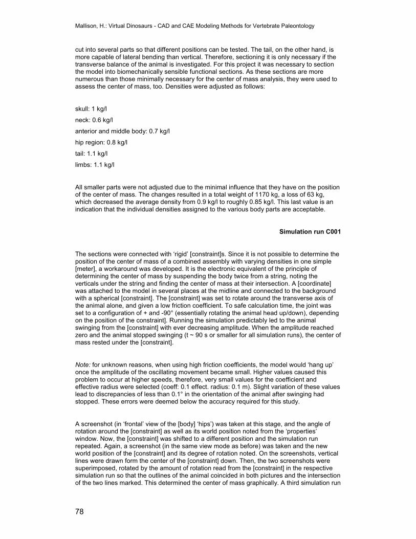
Mallison, H.: Virtual Dinosaurs - CAD and CAE Modeling Methods for Vertebrate Paleontology
78
cut into several parts so that different positions can be tested. The tail, on the other hand, is more capable of lateral bending than vertical. Therefore, sectioning it is only necessary if the transverse balance of the animal is investigated. For this project it was necessary to section the model into biomechanically sensible functional sections. As these sections are more numerous than those minimally necessary for the center of mass analysis, they were used to assess the center of mass, too. Densities were adjusted as follows:
skull: 1 kg/l
neck: 0.6 kg/l
anterior and middle body: 0.7 kg/l
hip region: 0.8 kg/l
tail: 1.1 kg/l
limbs: 1.1 kg/l
All smaller parts were not adjusted due to the minimal influence that they have on the position of the center of mass. The changes resulted in a total weight of 1170 kg, a loss of 63 kg, which decreased the average density from 0.9 kg/l to roughly 0.85 kg/l. This last value is an indication that the individual densities assigned to the various body parts are acceptable.
Simulation run C001
The sections were connected with ‘rigid’ [constraint]s. Since it is not possible to determine the position of the center of mass of a combined assembly with varying densities in one simple [meter], a workaround was developed. It is the electronic equivalent of the principle of determining the center of mass by suspending the body twice from a string, noting the verticals under the string and finding the center of mass at their intersection. A [coordinate] was attached to the model in several places at the midline and connected to the background with a spherical [constraint]. The [constraint] was set to rotate around the transverse axis of the animal alone, and given a low friction coefficient. To safe calculation time, the joint was set to a configuration of + and -90° (essentially rotating the animal head up/down), depending on the position of the constraint]. Running the simulation predictably led to the animal swinging from the [constraint] with ever decreasing amplitude. When the amplitude reached zero and the animal stopped swinging (t ~ 90 s or smaller for all simulation runs), the center of mass rested under the [constraint].
Note: for unknown reasons, when using high friction coefficients, the model would ‘hang up’ once the amplitude of the oscillating movement became small. Higher values caused this problem to occur at higher speeds, therefore, very small values for the coefficient and effective radius were selected (coeff: 0.1 effect. radius: 0.1 m). Slight variation of these values lead to discrepancies of less than 0.1° in the orientation of the animal after swinging had stopped. These errors were deemed below the accuracy required for this study.
A screenshot (in ‘frontal’ view of the [body] ‘hips’) was taken at this stage, and the angle of rotation around the [constraint] as well as its world position noted from the ‘properties’ window. Now, the [constraint] was shifted to a different position and the simulation run repeated. Again, a screenshot (in the same view mode as before) was taken and the new world position of the [constraint] and its degree of rotation noted. On the screenshots, vertical lines were drawn form the center of the [constraint] down. Then, the two screenshots were superimposed, rotated by the amount of rotation read from the [constraint] in the respective simulation run so that the outlines of the animal coincided in both pictures and the intersection of the two lines marked. This determined the center of mass graphically. A third simulation run
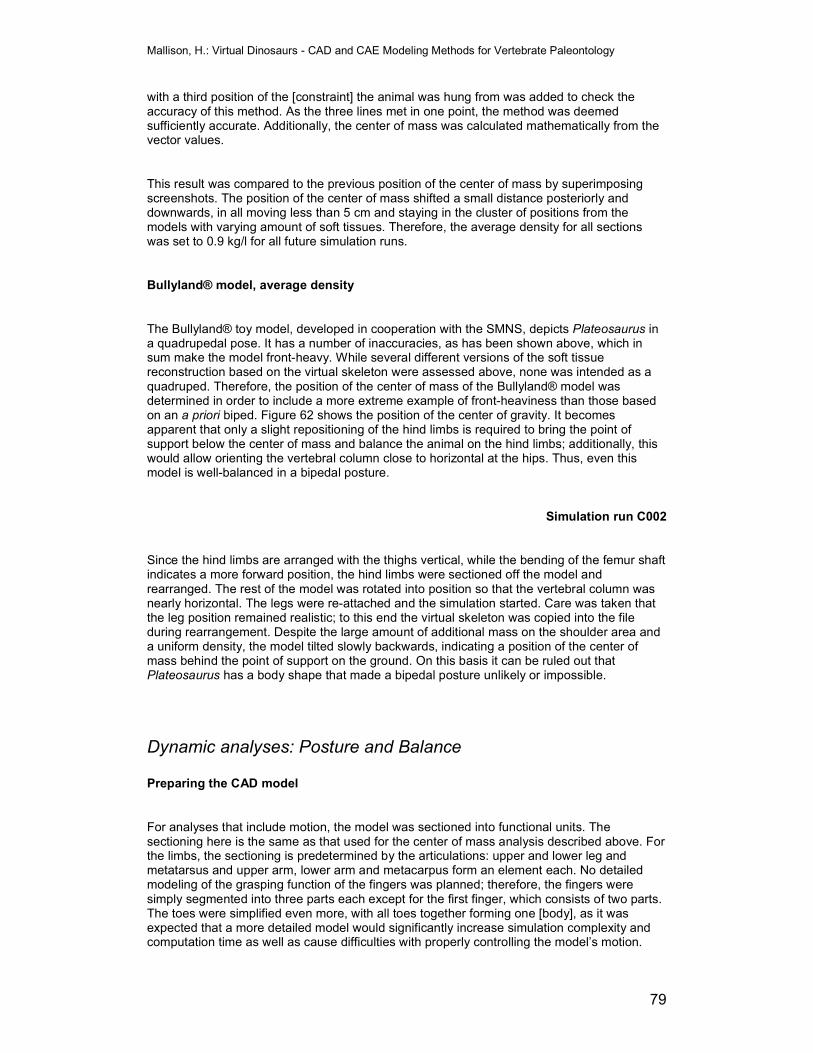
Mallison, H.: Virtual Dinosaurs - CAD and CAE Modeling Methods for Vertebrate Paleontology
79
with a third position of the [constraint] the animal was hung from was added to check the accuracy of this method. As the three lines met in one point, the method was deemed sufficiently accurate. Additionally, the center of mass was calculated mathematically from the vector values.
This result was compared to the previous position of the center of mass by superimposing screenshots. The position of the center of mass shifted a small distance posteriorly and downwards, in all moving less than 5 cm and staying in the cluster of positions from the models with varying amount of soft tissues. Therefore, the average density for all sections was set to 0.9 kg/l for all future simulation runs.
Bullyland® model, average density
The Bullyland® toy model, developed in cooperation with the SMNS, depicts Plateosaurus in a quadrupedal pose. It has a number of inaccuracies, as has been shown above, which in sum make the model front-heavy. While several different versions of the soft tissue reconstruction based on the virtual skeleton were assessed above, none was intended as a quadruped. Therefore, the position of the center of mass of the Bullyland® model was determined in order to include a more extreme example of front-heaviness than those based on an a priori biped. Figure 62 shows the position of the center of gravity. It becomes apparent that only a slight repositioning of the hind limbs is required to bring the point of support below the center of mass and balance the animal on the hind limbs; additionally, this would allow orienting the vertebral column close to horizontal at the hips. Thus, even this model is well-balanced in a bipedal posture.
Simulation run C002
Since the hind limbs are arranged with the thighs vertical, while the bending of the femur shaft indicates a more forward position, the hind limbs were sectioned off the model and rearranged. The rest of the model was rotated into position so that the vertebral column was nearly horizontal. The legs were re-attached and the simulation started. Care was taken that the leg position remained realistic; to this end the virtual skeleton was copied into the file during rearrangement. Despite the large amount of additional mass on the shoulder area and a uniform density, the model tilted slowly backwards, indicating a position of the center of mass behind the point of support on the ground. On this basis it can be ruled out that Plateosaurus has a body shape that made a bipedal posture unlikely or impossible.
Dynamic analyses: Posture and Balance Preparing the CAD model
For analyses that include motion, the model was sectioned into functional units. The sectioning here is the same as that used for the center of mass analysis described above. For the limbs, the sectioning is predetermined by the articulations: upper and lower leg and metatarsus and upper arm, lower arm and metacarpus form an element each. No detailed modeling of the grasping function of the fingers was planned; therefore, the fingers were simply segmented into three parts each except for the first finger, which consists of two parts. The toes were simplified even more, with all toes together forming one [body], as it was expected that a more detailed model would significantly increase simulation complexity and computation time as well as cause difficulties with properly controlling the model’s motion.
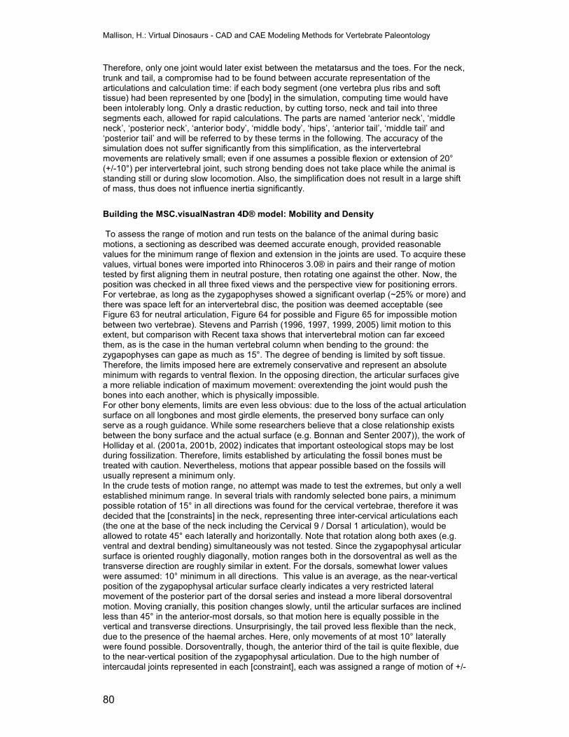
Mallison, H.: Virtual Dinosaurs - CAD and CAE Modeling Methods for Vertebrate Paleontology
80
Therefore, only one joint would later exist between the metatarsus and the toes. For the neck, trunk and tail, a compromise had to be found between accurate representation of the articulations and calculation time: if each body segment (one vertebra plus ribs and soft tissue) had been represented by one [body] in the simulation, computing time would have been intolerably long. Only a drastic reduction, by cutting torso, neck and tail into three segments each, allowed for rapid calculations. The parts are named ‘anterior neck’, ‘middle neck’, ‘posterior neck’, ‘anterior body’, ‘middle body’, ‘hips’, ‘anterior tail’, ‘middle tail’ and ‘posterior tail’ and will be referred to by these terms in the following. The accuracy of the simulation does not suffer significantly from this simplification, as the intervertebral movements are relatively small; even if one assumes a possible flexion or extension of 20° (+/-10°) per intervertebral joint, such strong bending does not take place while the animal is standing still or during slow locomotion. Also, the simplification does not result in a large shift of mass, thus does not influence inertia significantly.
Building the MSC.visualNastran 4D® model: Mobility and Density To assess the range of motion and run tests on the balance of the animal during basic motions, a sectioning as described was deemed accurate enough, provided reasonable values for the minimum range of flexion and extension in the joints are used. To acquire these values, virtual bones were imported into Rhinoceros 3.0® in pairs and their range of motion tested by first aligning them in neutral posture, then rotating one against the other. Now, the position was checked in all three fixed views and the perspective view for positioning errors. For vertebrae, as long as the zygapophyses showed a significant overlap (~25% or more) and there was space left for an intervertebral disc, the position was deemed acceptable (see Figure 63 for neutral articulation, Figure 64 for possible and Figure 65 for impossible motion between two vertebrae). Stevens and Parrish (1996, 1997, 1999, 2005) limit motion to this extent, but comparison with Recent taxa shows that intervertebral motion can far exceed them, as is the case in the human vertebral column when bending to the ground: the zygapophyses can gape as much as 15°. The degree of bending is limited by soft tissue. Therefore, the limits imposed here are extremely conservative and represent an absolute minimum with regards to ventral flexion. In the opposing direction, the articular surfaces give a more reliable indication of maximum movement: overextending the joint would push the bones into each another, which is physically impossible. For other bony elements, limits are even less obvious: due to the loss of the actual articulation surface on all longbones and most girdle elements, the preserved bony surface can only serve as a rough guidance. While some researchers believe that a close relationship exists between the bony surface and the actual surface (e.g. Bonnan and Senter 2007)), the work of Holliday et al. (2001a, 2001b, 2002) indicates that important osteological stops may be lost during fossilization. Therefore, limits established by articulating the fossil bones must be treated with caution. Nevertheless, motions that appear possible based on the fossils will usually represent a minimum only. In the crude tests of motion range, no attempt was made to test the extremes, but only a well established minimum range. In several trials with randomly selected bone pairs, a minimum possible rotation of 15° in all directions was found for the cervical vertebrae, therefore it was decided that the [constraints] in the neck, representing three inter-cervical articulations each (the one at the base of the neck including the Cervical 9 / Dorsal 1 articulation), would be allowed to rotate 45° each laterally and horizontally. Note that rotation along both axes (e.g. ventral and dextral bending) simultaneously was not tested. Since the zygapophysal articular surface is oriented roughly diagonally, motion ranges both in the dorsoventral as well as the transverse direction are roughly similar in extent. For the dorsals, somewhat lower values were assumed: 10° minimum in all directions. This value is an average, as the near-vertical position of the zygapophysal articular surface clearly indicates a very restricted lateral movement of the posterior part of the dorsal series and instead a more liberal dorsoventral motion. Moving cranially, this position changes slowly, until the articular surfaces are inclined less than 45° in the anterior-most dorsals, so that motion here is equally possible in the vertical and transverse directions. Unsurprisingly, the tail proved less flexible than the neck, due to the presence of the haemal arches. Here, only movements of at most 10° laterally were found possible. Dorsoventrally, though, the anterior third of the tail is quite flexible, due to the near-vertical position of the zygapophysal articulation. Due to the high number of intercaudal joints represented in each [constraint], each was assigned a range of motion of +/-
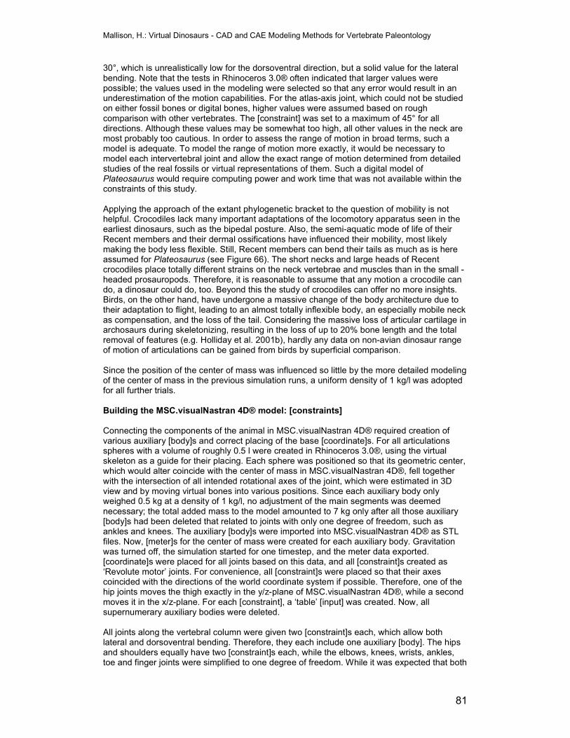
Mallison, H.: Virtual Dinosaurs - CAD and CAE Modeling Methods for Vertebrate Paleontology
81
30°, which is unrealistically low for the dorsoventral direction, but a solid value for the lateral bending. Note that the tests in Rhinoceros 3.0® often indicated that larger values were possible; the values used in the modeling were selected so that any error would result in an underestimation of the motion capabilities. For the atlas-axis joint, which could not be studied on either fossil bones or digital bones, higher values were assumed based on rough comparison with other vertebrates. The [constraint] was set to a maximum of 45° for all directions. Although these values may be somewhat too high, all other values in the neck are most probably too cautious. In order to assess the range of motion in broad terms, such a model is adequate. To model the range of motion more exactly, it would be necessary to model each intervertebral joint and allow the exact range of motion determined from detailed studies of the real fossils or virtual representations of them. Such a digital model of Plateosaurus would require computing power and work time that was not available within the constraints of this study. Applying the approach of the extant phylogenetic bracket to the question of mobility is not helpful. Crocodiles lack many important adaptations of the locomotory apparatus seen in the earliest dinosaurs, such as the bipedal posture. Also, the semi-aquatic mode of life of their Recent members and their dermal ossifications have influenced their mobility, most likely making the body less flexible. Still, Recent members can bend their tails as much as is here assumed for Plateosaurus (see Figure 66). The short necks and large heads of Recent crocodiles place totally different strains on the neck vertebrae and muscles than in the small -headed prosauropods. Therefore, it is reasonable to assume that any motion a crocodile can do, a dinosaur could do, too. Beyond this the study of crocodiles can offer no more insights. Birds, on the other hand, have undergone a massive change of the body architecture due to their adaptation to flight, leading to an almost totally inflexible body, an especially mobile neck as compensation, and the loss of the tail. Considering the massive loss of articular cartilage in archosaurs during skeletonizing, resulting in the loss of up to 20% bone length and the total removal of features (e.g. Holliday et al. 2001b), hardly any data on non-avian dinosaur range of motion of articulations can be gained from birds by superficial comparison. Since the position of the center of mass was influenced so little by the more detailed modeling of the center of mass in the previous simulation runs, a uniform density of 1 kg/l was adopted for all further trials. Building the MSC.visualNastran 4D® model: [constraints] Connecting the components of the animal in MSC.visualNastran 4D® required creation of various auxiliary [body]s and correct placing of the base [coordinate]s. For all articulations spheres with a volume of roughly 0.5 l were created in Rhinoceros 3.0®, using the virtual skeleton as a guide for their placing. Each sphere was positioned so that its geometric center, which would alter coincide with the center of mass in MSC.visualNastran 4D®, fell together with the intersection of all intended rotational axes of the joint, which were estimated in 3D view and by moving virtual bones into various positions. Since each auxiliary body only weighed 0.5 kg at a density of 1 kg/l, no adjustment of the main segments was deemed necessary; the total added mass to the model amounted to 7 kg only after all those auxiliary [body]s had been deleted that related to joints with only one degree of freedom, such as ankles and knees. The auxiliary [body]s were imported into MSC.visualNastran 4D® as STL files. Now, [meter]s for the center of mass were created for each auxiliary body. Gravitation was turned off, the simulation started for one timestep, and the meter data exported. [coordinate]s were placed for all joints based on this data, and all [constraint]s created as ‘Revolute motor’ joints. For convenience, all [constraint]s were placed so that their axes coincided with the directions of the world coordinate system if possible. Therefore, one of the hip joints moves the thigh exactly in the y/z-plane of MSC.visualNastran 4D®, while a second moves it in the x/z-plane. For each [constraint], a ‘table’ [input] was created. Now, all supernumerary auxiliary bodies were deleted. All joints along the vertebral column were given two [constraint]s each, which allow both lateral and dorsoventral bending. Therefore, they each include one auxiliary [body]. The hips and shoulders equally have two [constraint]s each, while the elbows, knees, wrists, ankles, toe and finger joints were simplified to one degree of freedom. While it was expected that both
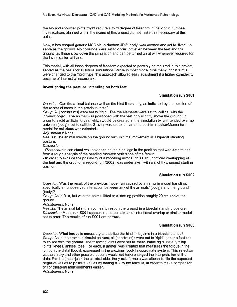
Mallison, H.: Virtual Dinosaurs - CAD and CAE Modeling Methods for Vertebrate Paleontology
82
the hip and shoulder joints might require a third degree of freedom in the long run, those investigations planned within the scope of this project did not make this necessary at this point. Now, a box shaped generic MSC.visualNastran 4D® [body] was created and set to ‘fixed’, to serve as the ground. No collisions were set to occur, not even between the feet and the ground, as these slow down the simulation and can be turned on at will whenever required for the investigation at hand. This model, with all those degrees of freedom expected to possibly be required in this project, served as the basis for all future simulations. While in most model runs many [constraint]s were changed to the ‘rigid’ type, this approach allowed easy adjustment if a higher complexity became of interest or necessary. Investigating the posture - standing on both feet
Simulation run S001
Question: Can the animal balance well on the hind limbs only, as indicated by the position of the center of mass in the previous tests? Setup: All [constraints] were set to ‘rigid’. The toe elements were set to ‘collide’ with the ‘ground’ object. The animal was positioned with the feet only slightly above the ground, in order to avoid artificial forces, which would be created in the simulation by unintended overlap between [body]s set to collide. Gravity was set to ‘on’ and the built-in Impulse/Momentum model for collisions was selected. Adjustments: None Results: The animal stands on the ground with minimal movement in a bipedal standing posture. Discussion: - Plateosaurus can stand well-balanced on the hind legs in the position that was determined from a rough analysis of the bending moment resistance of the femur. - In order to exclude the possibility of a modeling error such as an unnoticed overlapping of the feet and the ground, a second run (S002) was undertaken with a slightly changed starting position.
Simulation run S002 Question: Was the result of the previous model run caused by an error in model handling, specifically an unobserved interaction between any of the animals’ [body]s and the ‘ground’ [body]? Setup: As in B1a, but with the animal lifted to a starting position roughly 20 cm above the ground. Adjustments: None Results: The animal falls, then comes to rest on the ground in a bipedal standing posture. Discussion: Model run S001 appears not to contain an unintentional overlap or similar model setup error. The results of run S001 are correct.
Simulation run S003
Question: What torque is necessary to stabilize the hind limb joints in a bipedal stance? Setup: As in the previous simulation runs, all [constraint]s were set to ‘rigid’ and the feet set to collide with the ground. The following joints were set to ‘measurable rigid’ state: y/z hip joints, knees, ankles, toes. For each, a [meter] was created that measures the torque in the joint on the distal [body], expressed in the proximal [body]’s coordinate system. This selection was arbitrary and other possible options would not have changed the interpretation of the data. For the [meter]s on the sinistral side, the y-axis formula was altered to flip the expected negative values to positive values by adding a ‘-‘ to the formula, in order to make comparison of contralateral measurements easier. Adjustments: None.
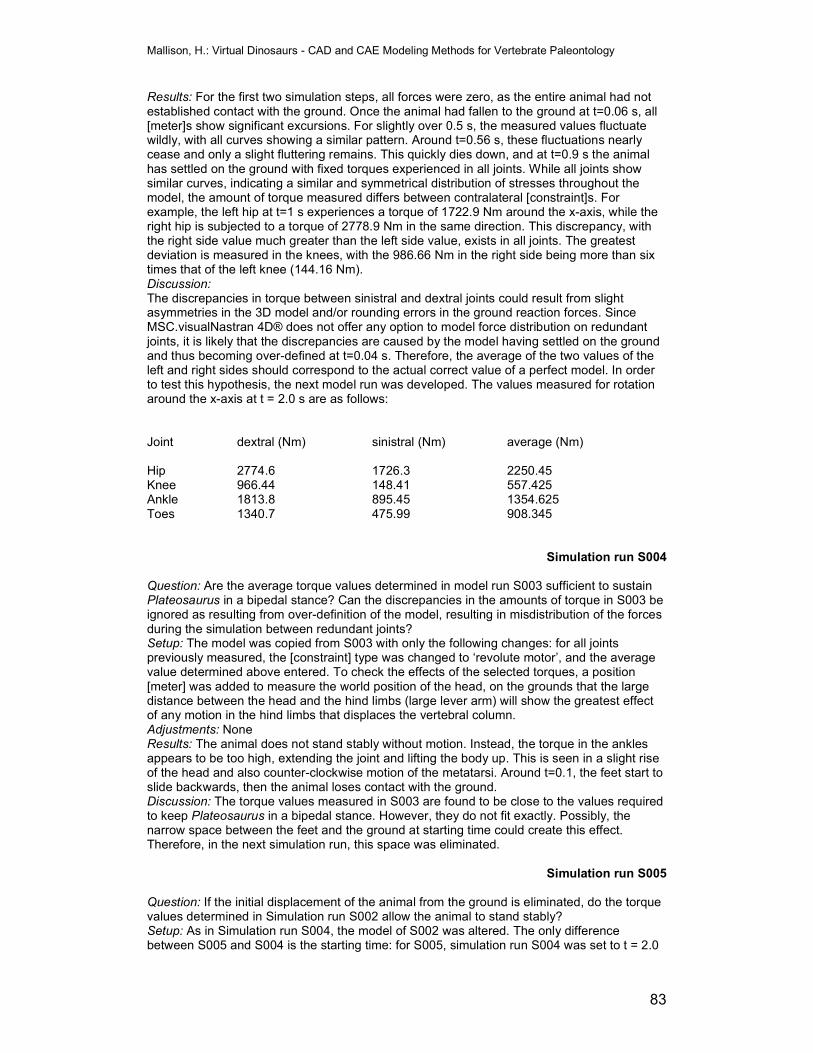
Mallison, H.: Virtual Dinosaurs - CAD and CAE Modeling Methods for Vertebrate Paleontology
83
Results: For the first two simulation steps, all forces were zero, as the entire animal had not established contact with the ground. Once the animal had fallen to the ground at t=0.06 s, all [meter]s show significant excursions. For slightly over 0.5 s, the measured values fluctuate wildly, with all curves showing a similar pattern. Around t=0.56 s, these fluctuations nearly cease and only a slight fluttering remains. This quickly dies down, and at t=0.9 s the animal has settled on the ground with fixed torques experienced in all joints. While all joints show similar curves, indicating a similar and symmetrical distribution of stresses throughout the model, the amount of torque measured differs between contralateral [constraint]s. For example, the left hip at t=1 s experiences a torque of 1722.9 Nm around the x-axis, while the right hip is subjected to a torque of 2778.9 Nm in the same direction. This discrepancy, with the right side value much greater than the left side value, exists in all joints. The greatest deviation is measured in the knees, with the 986.66 Nm in the right side being more than six times that of the left knee (144.16 Nm). Discussion: The discrepancies in torque between sinistral and dextral joints could result from slight asymmetries in the 3D model and/or rounding errors in the ground reaction forces. Since MSC.visualNastran 4D® does not offer any option to model force distribution on redundant joints, it is likely that the discrepancies are caused by the model having settled on the ground and thus becoming over-defined at t=0.04 s. Therefore, the average of the two values of the left and right sides should correspond to the actual correct value of a perfect model. In order to test this hypothesis, the next model run was developed. The values measured for rotation around the x-axis at t = 2.0 s are as follows: Joint dextral (Nm) sinistral (Nm) average (Nm) Hip 2774.6 1726.3 2250.45 Knee 966.44 148.41 557.425 Ankle 1813.8 895.45 1354.625 Toes 1340.7 475.99 908.345
Simulation run S004
Question: Are the average torque values determined in model run S003 sufficient to sustain Plateosaurus in a bipedal stance? Can the discrepancies in the amounts of torque in S003 be ignored as resulting from over-definition of the model, resulting in misdistribution of the forces during the simulation between redundant joints? Setup: The model was copied from S003 with only the following changes: for all joints previously measured, the [constraint] type was changed to ‘revolute motor’, and the average value determined above entered. To check the effects of the selected torques, a position [meter] was added to measure the world position of the head, on the grounds that the large distance between the head and the hind limbs (large lever arm) will show the greatest effect of any motion in the hind limbs that displaces the vertebral column. Adjustments: None Results: The animal does not stand stably without motion. Instead, the torque in the ankles appears to be too high, extending the joint and lifting the body up. This is seen in a slight rise of the head and also counter-clockwise motion of the metatarsi. Around t=0.1, the feet start to slide backwards, then the animal loses contact with the ground. Discussion: The torque values measured in S003 are found to be close to the values required to keep Plateosaurus in a bipedal stance. However, they do not fit exactly. Possibly, the narrow space between the feet and the ground at starting time could create this effect. Therefore, in the next simulation run, this space was eliminated.
Simulation run S005 Question: If the initial displacement of the animal from the ground is eliminated, do the torque values determined in Simulation run S002 allow the animal to stand stably? Setup: As in Simulation run S004, the model of S002 was altered. The only difference between S005 and S004 is the starting time: for S005, simulation run S004 was set to t = 2.0
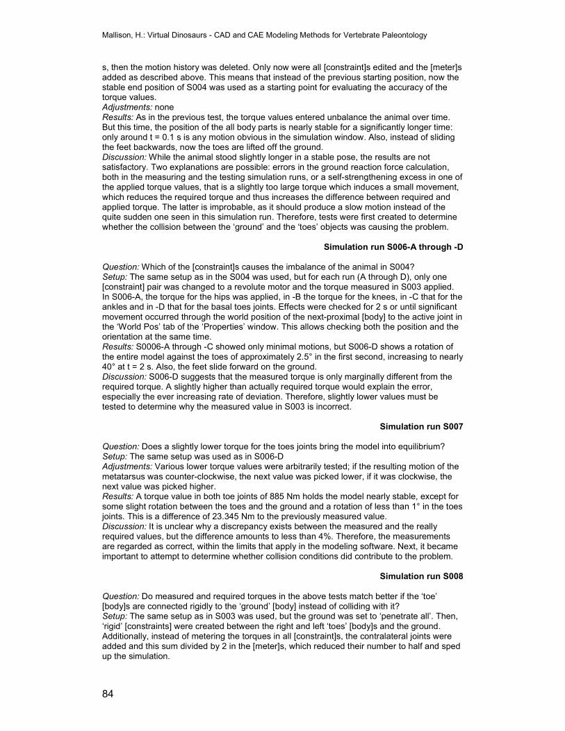
Mallison, H.: Virtual Dinosaurs - CAD and CAE Modeling Methods for Vertebrate Paleontology
84
s, then the motion history was deleted. Only now were all [constraint]s edited and the [meter]s added as described above. This means that instead of the previous starting position, now the stable end position of S004 was used as a starting point for evaluating the accuracy of the torque values. Adjustments: none Results: As in the previous test, the torque values entered unbalance the animal over time. But this time, the position of the all body parts is nearly stable for a significantly longer time: only around t = 0.1 s is any motion obvious in the simulation window. Also, instead of sliding the feet backwards, now the toes are lifted off the ground. Discussion: While the animal stood slightly longer in a stable pose, the results are not satisfactory. Two explanations are possible: errors in the ground reaction force calculation, both in the measuring and the testing simulation runs, or a self-strengthening excess in one of the applied torque values, that is a slightly too large torque which induces a small movement, which reduces the required torque and thus increases the difference between required and applied torque. The latter is improbable, as it should produce a slow motion instead of the quite sudden one seen in this simulation run. Therefore, tests were first created to determine whether the collision between the ‘ground’ and the ‘toes’ objects was causing the problem.
Simulation run S006-A through -D
Question: Which of the [constraint]s causes the imbalance of the animal in S004? Setup: The same setup as in the S004 was used, but for each run (A through D), only one [constraint] pair was changed to a revolute motor and the torque measured in S003 applied. In S006-A, the torque for the hips was applied, in -B the torque for the knees, in -C that for the ankles and in -D that for the basal toes joints. Effects were checked for 2 s or until significant movement occurred through the world position of the next-proximal [body] to the active joint in the ‘World Pos’ tab of the ‘Properties’ window. This allows checking both the position and the orientation at the same time. Results: S0006-A through -C showed only minimal motions, but S006-D shows a rotation of the entire model against the toes of approximately 2.5° in the first second, increasing to nearly 40° at t = 2 s. Also, the feet slide forward on the ground. Discussion: S006-D suggests that the measured torque is only marginally different from the required torque. A slightly higher than actually required torque would explain the error, especially the ever increasing rate of deviation. Therefore, slightly lower values must be tested to determine why the measured value in S003 is incorrect.
Simulation run S007 Question: Does a slightly lower torque for the toes joints bring the model into equilibrium? Setup: The same setup was used as in S006-D Adjustments: Various lower torque values were arbitrarily tested; if the resulting motion of the metatarsus was counter-clockwise, the next value was picked lower, if it was clockwise, the next value was picked higher. Results: A torque value in both toe joints of 885 Nm holds the model nearly stable, except for some slight rotation between the toes and the ground and a rotation of less than 1° in the toes joints. This is a difference of 23.345 Nm to the previously measured value. Discussion: It is unclear why a discrepancy exists between the measured and the really required values, but the difference amounts to less than 4%. Therefore, the measurements are regarded as correct, within the limits that apply in the modeling software. Next, it became important to attempt to determine whether collision conditions did contribute to the problem.
Simulation run S008 Question: Do measured and required torques in the above tests match better if the ‘toe’ [body]s are connected rigidly to the ‘ground’ [body] instead of colliding with it? Setup: The same setup as in S003 was used, but the ground was set to ‘penetrate all’. Then, ‘rigid’ [constraints] were created between the right and left ‘toes’ [body]s and the ground. Additionally, instead of metering the torques in all [constraint]s, the contralateral joints were added and this sum divided by 2 in the [meter]s, which reduced their number to half and sped up the simulation.
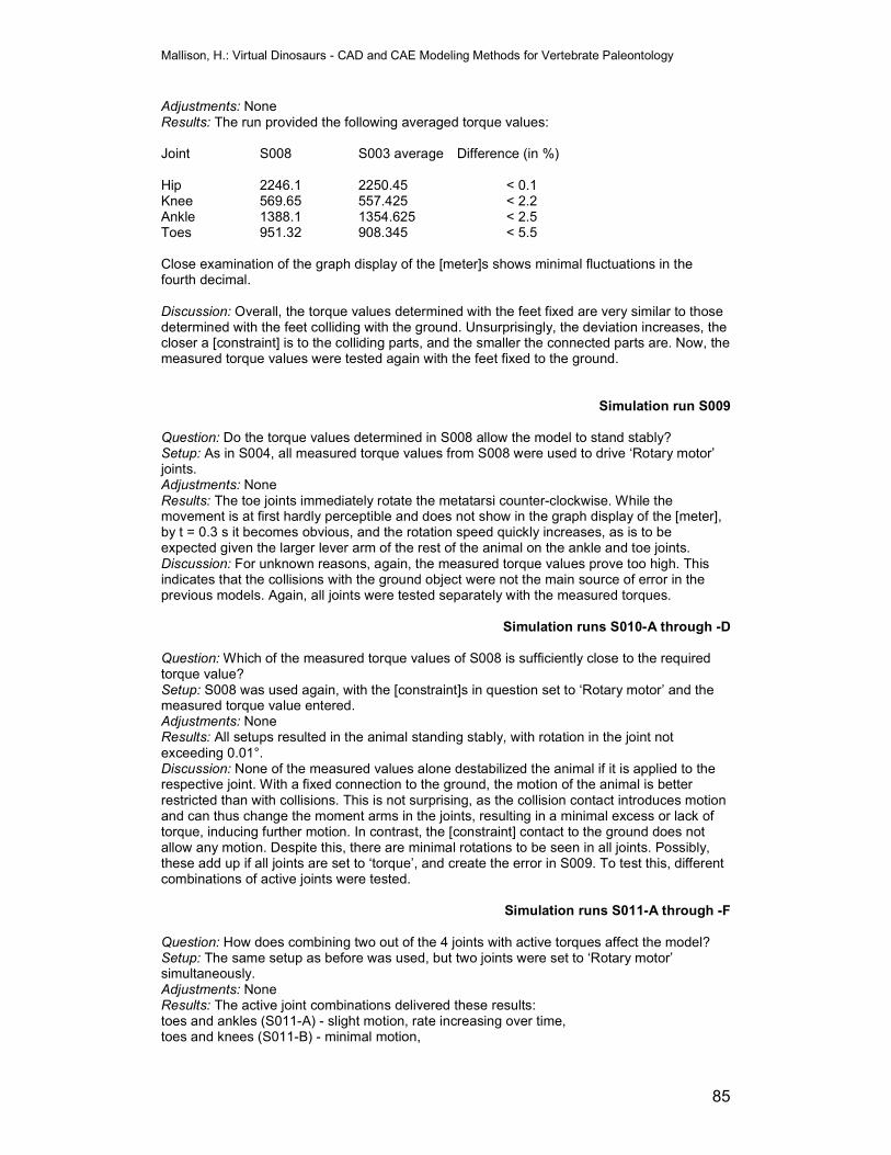
Mallison, H.: Virtual Dinosaurs - CAD and CAE Modeling Methods for Vertebrate Paleontology
85
Adjustments: None Results: The run provided the following averaged torque values: Joint S008 S003 average Difference (in %) Hip 2246.1 2250.45 < 0.1 Knee 569.65 557.425 < 2.2 Ankle 1388.1 1354.625 < 2.5 Toes 951.32 908.345 < 5.5 Close examination of the graph display of the [meter]s shows minimal fluctuations in the fourth decimal. Discussion: Overall, the torque values determined with the feet fixed are very similar to those determined with the feet colliding with the ground. Unsurprisingly, the deviation increases, the closer a [constraint] is to the colliding parts, and the smaller the connected parts are. Now, the measured torque values were tested again with the feet fixed to the ground.
Simulation run S009 Question: Do the torque values determined in S008 allow the model to stand stably? Setup: As in S004, all measured torque values from S008 were used to drive ‘Rotary motor’ joints. Adjustments: None Results: The toe joints immediately rotate the metatarsi counter-clockwise. While the movement is at first hardly perceptible and does not show in the graph display of the [meter], by t = 0.3 s it becomes obvious, and the rotation speed quickly increases, as is to be expected given the larger lever arm of the rest of the animal on the ankle and toe joints. Discussion: For unknown reasons, again, the measured torque values prove too high. This indicates that the collisions with the ground object were not the main source of error in the previous models. Again, all joints were tested separately with the measured torques.
Simulation runs S010-A through -D
Question: Which of the measured torque values of S008 is sufficiently close to the required torque value? Setup: S008 was used again, with the [constraint]s in question set to ‘Rotary motor’ and the measured torque value entered. Adjustments: None Results: All setups resulted in the animal standing stably, with rotation in the joint not exceeding 0.01°. Discussion: None of the measured values alone destabilized the animal if it is applied to the respective joint. With a fixed connection to the ground, the motion of the animal is better restricted than with collisions. This is not surprising, as the collision contact introduces motion and can thus change the moment arms in the joints, resulting in a minimal excess or lack of torque, inducing further motion. In contrast, the [constraint] contact to the ground does not allow any motion. Despite this, there are minimal rotations to be seen in all joints. Possibly, these add up if all joints are set to ‘torque’, and create the error in S009. To test this, different combinations of active joints were tested.
Simulation runs S011-A through -F
Question: How does combining two out of the 4 joints with active torques affect the model? Setup: The same setup as before was used, but two joints were set to ‘Rotary motor’ simultaneously. Adjustments: None Results: The active joint combinations delivered these results: toes and ankles (S011-A) - slight motion, rate increasing over time, toes and knees (S011-B) - minimal motion,
Mallison, H.: Virtual Dinosaurs - CAD and CAE Modeling Methods for Vertebrate Paleontology
86
toes and hips (S011-C) - minimal motion, ankles and knees (S011-D) - slight counterclockwise rotation in the ankle, ankles and hips (S011-E) - minimal motion, knees and hips (S011-F) - minimal motion. Discussion: No coherent pattern appears. Possibly, the ankle torque value is not exact enough to guarantee stability, but this can not be determined from this data. It appears that measuring torques in ‘measurable rigid’ joints is an acceptable way of determining torques, but errors up to several percent must be expected. Possibly, a mathematical formula aimed at correcting deviations instead of a simple value allows better control of the model.
Simulation run S012
Question: Is it possible to achieve a self-correcting pose, in which a mathematical formula adjusts the torque so that the orientation of the joint is corrected if it deviates from the starting position? Setup: The same setup as in S010-A was used, but instead of a fixed torque value, the formula
if(constraint[133].r.x<-1,2256.1,if(constraint[133].r.x<-
0.5,2251.1,if(constraint[133].r.x<0.5,2241.6,2236.1))) was entered. It is a simple step function based on three true/false decisions. It assigns a torque value larger than necessary for equilibrium if the [constraint] rotates so that the moment arm of the [body]s supported by it increases, and a smaller torque value if the [constraint] rotation decreases the load on itself. These values were stepped to allow a greater correction for larger deviations, with a +/-5 Nm difference at +/-0.5° and a +/-10 Nm difference at +/-1°. A [meter] was used to measure the orientation of the left hip joint. Adjustments: None Results: The orientation of the hip changes following a sinusoidal curve with a period of 5.44 s, an amplitude of 0.629° and an average of -0.315°. Discussion: The simple formula proved sufficient to control the model well, but the average position of the [constraint] fell by 0.315°. As this formula also counters a variable deviation with fixed values only, the next simulation run attempted to scale the correction according to the deviation.
Simulation run S013 Question: Can a formula be found that exerts tighter control over the [constraint] orientation? Setup: The same setup as in S013 was used, and the formula changed to:
a+sin(constraint[133].r.x)*(-b) N m It applies a base torque (a) as determined in S008 (here: 22146.1 Nm), and adds a correction torque that depends on the amount of rotation of the joint. This correction factor consists of the sinus of the [constraint]’s orientation multiplied with a factor b. The latter is necessary, as the sinus curve only varies between -1 and 1. In this case, a negative b is required, due to the setup of the [constraint] coordinate system. The higher b is, the higher the countering force will be. As long as the deviation stays within +/-π/2, a growing deviation is countered by a growing correction factor. Adjustments: Various values were tested for the factor b, with b=10, b=100 and b=1000 delivering similar results. Results: The hip orientation varies following a sinusoidal curve with a period of 1.5 s and an amplitude of 0.0002°. The average [constraint] orientation is -0.0001° Discussion: A sinusoidal function appears to be a simple and effective tool of controlling a [constraint] tightly. Next, tests were undertaken to determine if combining several such control inputs produces interference.
Simulation run S014-A through -C
Mallison, H.: Virtual Dinosaurs - CAD and CAE Modeling Methods for Vertebrate Paleontology
87
Question: Can formulae such as that used in S013 be used in several neighboring [constraint]s at the same time without interference? Setup: The same setup as in S013 was used, and one by one, more distal joints were additionally controlled with formula following this pattern:
a+sin(constraint[133].r.x)*(-b) N m In S014-A, both the hips and the knees were controlled this way, S014-B added the ankles, and S014-C added the toes joints. Adjustments: Various values for b were tested in all formulae. In an attempt to determine the cause of problems with S014-C, a [meter] to measure the torque was created for various joints. Results: In S014-A, both the hip and knee joints exhibit a complex motion, following a curve consisting of combined sinusoidal curves. Both show a main period of 2.1 s, and second, superimposed period of 0.7 s. As is to be expected, the two joints are offset by half a period, with the knee at a maximum when the hip is at a minimum. The total amplitude in both joints is 0.0002°. In S014-B, all three joints exhibit an even more complicated pattern of combined sinusoidal curves. The main period is roughly 2.4 s, and the total amplitude amounts to 0.0002° for knees and ankles again, and to 0.00008° for the ankles. S015-C never reaches a stable oscillating state. Various values for ‘b’ in all joint formulae were used, and higher values tended to produce better results up to values around 10000 Nm. Any further increase did not improve the results. All four joint orientation [meter]s zigzag wildly, but even the best test results show the curve change from a near-sinusoidal oscillation to an exponential curve at around t = 0.4 s. Discussion: As S014-A and -B show, controlling several neighboring [constraint]s with simple formulae is possible. S014-C proves that problems can arise unexpectedly, as only one more pair of joints was added compared to S014-B. What causes these problems is unknown. The deviation values at which the curves turn from sinusoidal to exponential are solidly within the range of +/-π/2, in which there should be adequate countering torques available. It does not seem likely that a simple combination of various rounding errors or a similar inaccuracy can lead the model into uncontrollable motion. Investigating the balance Any biped must not only be able to stand stably on one or both legs, but must also be able to move body parts, sometimes rapidly, without unbalancing this pose. A narrow base, with the feet close to the midline, and a high position of the center of mass make tipping more likely, while a broad base and a low center of mass make the pose more stable. But a broad base comes at a price: increasing abduction of the hindlimbs places an increasing torque on the hip joints, which must be countered by muscle action. Various positions were now tested and the required torques measured.
Simulation run S015-A through -F
Question: What transverse torques must to be countered in the hip joints for varying splaying angles of the hindlimbs? Setup: In the basic model, all [constraint]s were set to ‘Rotary motor’ type except for the ‘transverse’ hip joints and the ankle joints. These were set to govern adduction and abduction of the hind limbs as ‘measurable rigid’ [constraints]. Several different orientation values were tested: -10°, which placed the middle of the foot on the midline (S015-A), -4°, at which the feet touch at the midline (S015-B), 0°, which places the hindlimbs nearly vertically (S015-C), 5°, which splays the hindlimbs slightly (S015-D), 10°, which splays the hindlimbs more (S015-E) and 15°, which splays the hindlimbs extremely in a pose that elephants use for urinating (S015-F). Note that 0° corresponds to vertical, which not necessarily conforms to the neutral posture of the animal. Greater values were not tested, as it is probably not possible to abduct the femur any further, certainly not if there are loads active on the hip joints. To set these values,
Mallison, H.: Virtual Dinosaurs - CAD and CAE Modeling Methods for Vertebrate Paleontology
88
configuration was changed to the desired value and the desired orientation was set to the same value in the ‘Motor’ tab of the ‘Properties’ window. The feet were set to collide with the ground, and a [meter] was created that measured both the left and right hip torques on the y-axis and averaged them. Abduction or adduction of the entire hindlimb also rotates the soles of the feet, so that they are no longer parallel with the ground. This means that ground contact is only established along a thin line instead of a large area, since the ‘toes’ [body]s can not deform. No attempt was made to correct for this; rather, small movements caused by this problem were accepted, as no significant influence on the torques in the hips was expected. Adjustments: The initial setup resulted in inexplicable values, probably caused be the shift of the contact point between feet and ground on the feet. To eliminate this, the ankle joints were set to ‘Rotary motor’, with the y-axis as the rotation axis, and deflected to the same amount and in the opposite direction as the hip joints. This kept the soles of the feet level. This effectively removed whatever problem had caused the faulty results. In several trials, the animal rotated backwards around the x-axis and settled on the posterior end of the toe [body]s. A ‘generic’ [constraint] was added between the feet and the ground to stop this motion. Results: Moving the hindlimbs means that the model does not start the simulation in contact with the ground. All simulation runs show an initial phase of fluctuation torque values, but all settle quickly into a phase of relative stability. The values below stem from these periods. The following values were determined, rounded to full Nm: S015-A: 1838 Nm S015-B: 1106 Nm S015-C: 615 Nm S015-D: 0 Nm S015-E: -611 Nm S015-F: -1212 Nm Discussion: Placing the feet close to the midline requires strong abduction in the hip to keep the animal in balance. Splaying the limbs out requires significant adduction. The results fit prediction, indicating that at this level of complexity, the simulation is accurate. It becomes apparent that a slight abduction of the hindlimbs by 5° offers a balance of moments in the hip, making this position the least energy consuming as long as the animal stands still. Also, this position is inherently more stable than a narrower stance if lateral accelerations are considered.
Dynamic analyses: motions of the neck and tail versus the body, range of motion In addition to the above considerations, rapid movements of most body parts should not destabilize the posture of an animal. A support on only two points is inherently less stable than on four. Elephants, for example, while able to stand and even walk slowly in a bipedal stance, can not move rapidly or execute turns, nor can they sustain the position for extended times. Various different aspects must be considered. For one thing, aside from locomotion, animals must be able to stand up, lie down, drink, feed, etc. Some of these motions, especially getting up from a resting position or moving the head back up from ground level after drinking, can be involved in escape strategies, and must be conducted rapidly. Rapid motion, though, requires large accelerations and creates large amounts of rotational inertia. Therefore, such accelerations must be tested as well. As complex motion require complex controlling of the simulation and may not equate to maximum accelerations, several hypothetical scenarios were created to explore the maximum frame of possible motions. First, lateral motions of the vertebral column were tested, simulation the animal looking around, then suddenly deciding to straighten (e.g. in preparation for flight). This test was run on only one hindlimb orientation (0° abduction), to arrive at a conservative result. In reality, animals will widen their support base when engaging in rapid lateral motions. Then, vertical bending was tested, by simulating the animal drinking from a ground water source and snapping the head back up rapidly in preparation of flight. First, a deliberate attempt was made to topple the animal, even if this required improbable acceleration of body parts, then a slower and
Mallison, H.: Virtual Dinosaurs - CAD and CAE Modeling Methods for Vertebrate Paleontology
89
softer motion was created. These tests are not a rigorous modeling designed to deliver specific values, but rather serve as a check whether unexpected problems arise when the model is led through motions that are expected to be easily possible. Due to time constraints it was decided a priori to limit this to qualitative tests, more to assess the software capability than to create meaningful data on Plateosaurus. The description is given here for the sake of completeness.
Simulation run S016-A through -H
Question: Does rapid lateral bending destabilize the animal in a bipedal pose?
Setup: In the basic model, the base of the neck, the base of the tail plus the [constraint] connecting the first two tail segments and the two [constraint]s connecting the torso parts were set to ‘Rotary motor’. In each case, all connection points harbor two [constraint]s, in order to allow rotation around two axes simultaneously, but only one was used in this test. The [constrain]s were all set to rotate around the z-axis and slider [input]s were created to control them. These were set to range from -30° to 30°, in 60 steps, with 0° corresponding to the neutral position of the [constraint]. All other [constraint]s were set to ‘rigid’. A new [constraint] was created between the left toes and the ground, restricting motion in the x/y-plane, to simulate friction. Several [meter]s were created to measure the position of two newly created [coordinate]s on the soles of the feet, the angular velocity of the tail base [constraint] and the velocity of the tip of the tail.
S016-A
Adjustments: After the simulation was started, the slider controls were used to rotate body parts. All joints were moved so that the animal bent to the right side. All joints were rotated by 30°. In all, this meant that the head and the tip of the tail now only enclosed an angle of 30°. After the simulation had arrived at that position, all sliders were simultaneously set to 0° again, and then to a same value in the reverse direction.
Results: Initially, the animal rotates both the anterior body and neck and the tail to the right, while it tilts slightly to the left due to the transfer of rotational inertia. Once the desired position is reached, the internal motion stops abruptly, and a further transfer of inertia tilts the animal to the right and out of a stable position. The resulting fall is further sped up by the rotation to the contralateral side, which further accelerates the speed of the central body part.
Discussion: While it is possible to destabilize the animal by rapid lateral motions, it requires massive acceleration and deceleration of body parts. The tip of the tail reaches speeds of over 100 m/s (360 km/h) and the base of the tail reaches an angular velocity of 840.99 deg, equivalent to full 2.3 rotations per second! It is interesting to note that the animal does not start to fall before the rapid deceleration of body parts, indicating that even with tail and anterior body and neck turned to one side, the center of mass appears not to leave the support base laterally.
S016-B
Adjustments: After the simulation was started, the slider controls were used to rotate body parts. All joints were moved so that the animal bent to the right side. In contrast to S017-A, the motion was created with incremental adjustments. All joints were rotated by 30° as the final value. In all, this meant that the head and the tip of the tail now only enclosed an angle of 30° but the arresting of the motion was softer.
Results: The animal moves the body, neck and tail to the right. It sways somewhat from side to side, but ends in a stable position.
Note: some rapid ‘twitching’ motions to the left are caused by entering the data input numerically while the simulation is running. If a simulation step is started while the first digit of
Mallison, H.: Virtual Dinosaurs - CAD and CAE Modeling Methods for Vertebrate Paleontology
90
a two digit number has been typed, but the second digit is still missing, the next motion step in the simulation will use the first digit only. Changing the input from ‘20’ to ‘30’ may hence result in the simulation using the value ‘3’ for the duration of one simulation step.
Discussion: The test result indicates that Plateosaurus could move the tail and anterior body quickly without endangering the stability of a bipedal posture. Obviously, a broadening of the support base by abduction of the hind limbs could always be used to avoid a fall, but this simulation run shows that Plateosaurus did not have to depart from a neutral and energetically efficient nearly vertical limb position to conduct rapid lateral motions.
S016-C
Adjustments: In this test, the tail and body were deflected in the same direction instead of the same side. Additionally, the prepared [constraint]s within the tail and were used, their values controlled by the slider [input]s for the tail base and neck base, respectively. The maximum excursion tested was 25 ° for the neck and tail and 10° for the two joints in the torso.
Results: The animal rotates around the vertical axis whenever components are accelerated or decelerated.
Discussion: This model illustrates perfectly the problems that arise from the insufficient ability to control contacts between [body]s in MSC.visualNastran 4D®. While it is a realistic result that the animal counters the rotational forces acting on the limbs because of the transfer of rotational inertia from the tail and neck by rotating the body, it should be necessary to either rotate the limbs against the body or have the animal take small steps. Instead, the feet simply slide as if the animal wore skates on ice. Potentially, it may give more meaningful results to tie the feet to the ground with a generic constraint and measure the forces acting on it.
S016-D
Adjustments: In this and further tests, the various joints in the neck were given separate input controls to allow a more differentiated motion pattern. Motions around the transverse axes were introduced with the sliders, with to body at first straightening, then rapidly bending. Also the tail is lifted at the base before it is lowered. For a moment the model extends the back in a position reminiscent of the so-called ‘death pose’ known from many articulated finds. Then, body and neck curve down.
Discussion: The rapid accelerations of body parts far from the center of mass produce sufficient rotational inertia to repeatedly lift the animal a small distance off the ground. Also, it tilts backwards a bit, until the toes [body]s establishes better contact with the ground. The ‘jumps’ are not realistic, but rather are caused by simulation artifacts induced by the collision condition between the feet and the ground. The tail reaches a 285 deg rotation rate at the base, and a velocity of over 33 m/s. Despite this, the animal does not fall either forward or backward. Therefore, it can be concluded that these motions are well within the repertoire possible for Plateosaurus.
S016-E
Adjustments: The sliders were moved to conservative values for dorsally directed bending, this time slower than in S017-D to avoid lifting the animal off the ground. The tail was lifted at the same time as the neck was lowered, and vice versa. As the position of the zygapophyses in the tail indicates a limited ability to lift it, the maximum value used was 10°. Also, turning the tail down was limited to 10° at the base and 4° for the other joints, as this brought the tip down to ground level.
Results: The animal remains stable.
Discussion: Despite the fact that the tail base reaches rotation speeds of up to 470°/s, the animal stands stably. Again, it can be concluded that the bipedal posture is stable.
Mallison, H.: Virtual Dinosaurs - CAD and CAE Modeling Methods for Vertebrate Paleontology
91
S016-F
Adjustments: The sliders were moved to conservative values for dorsally directed bending in an attempt to move the head to the ground.
Results: The animal nearly reaches the ground, with the tip of the snout staying roughly 10 cm above it.
Discussion: It is unrealistic to assume that a potential prey animal is incapable of drinking unless it sits or lies down. While some animals, like giraffes, have to adopt uncomfortable positions in which they are incapable of rapid flight, e.g. due to the wide stance in the forelimbs that is required to bring a giraffe’s head to ground level, this is much safer than lowering the entire torso. The fact that the Plateosaurus model can not quite reach the ground may be caused by a conservative estimate of neck mobility. Additional bending of the dorsal vertebral column and rotation around the hip joints can help to cover the gap.
S016-G
Adjustments: Again, the neck was turned down, but this time the two [constraint]s in the torso were also rotated by 7°. The hips were given a slider [input] and rotated so that the anterior torso moved down by 10°.
Results: Bending the back and rotating the hip brings the tip of the snout comfortably down to ground level. Incidentally, this also lowers the center of mass a small distance, making the stance more stable. The animal again makes tiny ‘jumps’ directly after rapid accelerations.
Discussion: As before, ground reaction force modeling proves insufficient, despite the here much softer accelerations. If the model is not disarticulated, this test shows that Plateosaurus was able to drink or feed on the ground in a bipedal standing posture.
S016-H
Adjustments: The positions of the hips and the thigh at the start of the last simulation run were noted, and the virtual files of the left femur and the left side of the pelvic girdle imported and moved to that position. The virtual bones were attached to the respective soft tissue parts and the previous simulation recreated. The 3D model parts were hidden. This allows judging the motion of the skeletal elements during the sequence.
Results: The femoral protraction required to bring the head to the ground does not disarticulate the hip. The femur always stays behind the pubis, allowing the pubofemoral musculature to contribute to controlling the position.
Discussion: It can be concluded that the motions tested are well within the repertoire possible for Plateosaurus. While for this motion the information gained from adding the virtual bones is irrelevant, this test shows how easily virtual bones can be integrated into the simulation to check for inaccuracies. The only drawbacks are a higher number of components and slower computation times.
Simulation run S017-A through -D
Question: Can a motion sequence be developed for lying down and rising from a rest position?
Setup: In the basic model, the required joints were fitted with table [input]s. For S018-B and -D, the model was positioned in a resting pose on the ground similar to the position of the ‘sitting’ skeleton ‘F.33’ at the SMNS. Also, [meter]s were added to measure the torque in all limb joints in this test.
Mallison, H.: Virtual Dinosaurs - CAD and CAE Modeling Methods for Vertebrate Paleontology
92
S017-A and -C
Adjustments: Starting with the bipedal standing position, the tables were edited to show a motion sequence of the animal lying down, including a shift of the weight from one foot to the other to allow for adjusting the feet on the ground. Care was taken to model a slow and controlled descent.
Results: While the animal does squat down, an error in judgment led to an impractical position of the limb elements when the belly nears the ground: the metatarsus stays off the ground because the feet were protracted too little earlier in the motion sequence, and this forces the knee into a very high position. This, in turn, forces an extreme protraction of the thigh.
Discussion: As the exact sequence of how Plateosaurus can lie down on the ground is not important, it was decided to abort the model editing and let it serve as an example of how easily a pretty animation or simulation can become unrealistic. To emphasize the point, in S018-C the virtual bones of the left hindlimb and the left side of the pelvic girdle were copied in.
S017-B and -D
Adjustments: As in S018-A, the tables were edited to produce the desired motion. The animal was supposed to rise form the ground and start rapid locomotion. Hence, the knees would not be straightened to a fully standing pose, and one hindlimb would have to be lifted off the ground significantly. Also, the animal ideally should lean forward a bit.
Results: A sequence was developed that moves the animal from the resting position to a running position in 1.24 s. The center of gravity is placed well forward of the point of support at the end of the sequence.
The issue of mobility could be further investigated up by repeating the simulations with a more detailed model, which should incorporate the virtual bones of Plateosaurus and [constraint]s placed for each intervertebral joint. The maximum range of motion for each joint would have to be defined individually. Though time-consuming to create and requiring massive computing power, such a model could greatly aid in modeling the motion capabilities of Plateosaurus and closely related taxa.
Dynamic analyses: locomotion cycles All tetrapods use cyclic motions of their limbs and spine to move from one place to another. For those with parasagittal legs, the main aspect of locomotion is the anteroposterior movement of the limbs. Other aspects, such as the adduction and abduction of limbs to bring the point of support under the center of mass or lateral and vertical bending along the vertebral column to counter rotational inertia, are important contributions to conserving energy, but remain secondary issues to the cycle of extension and retraction of the limbs. Any attempt to model locomotion of an animal with parasagittal limbs must therefore center portraying the rotation of limb joints on transverse axes. All other issues can only be addressed once this goal has been achieved. Accordingly, a walking cycle limited to this motion was created first, using the procedure described above. Then, it was refined to determine if this procedure is suited for research on energy expenditure during locomotion.
Simulation run S018-A through -I
Question: What minimum data is necessary to design a realistic single step motion that can serve as a base for further research?
Mallison, H.: Virtual Dinosaurs - CAD and CAE Modeling Methods for Vertebrate Paleontology
93
Setup: In the basic model, all [constraint]s in the forelimbs and along the vertebral column were set to ‘rigid’. Also, the joints for adduction and abduction of the hindlimbs were made immobile. A ‘generic’ [constraint] was used to tie one foot to the ground, inhibiting both sliding and rotation in on all axes. The [constraint] orientations were now altered to place the model so that one hindlimb was fully extended and the toes just making contact with the ground, while the other limb, connected to the ground, was almost fully retracted. This corresponds to the ‘Initial contact’ position for the extended limb and the ‘Opposite Initial contact’ for the retracted limb and covers one step. The deflection values for all joints were copied into a MS EXCEL® table. Arbitrarily, it was decided that the full cycle should last 2 s, a slow walk, so for each [constraint] the value of the mirror joint at t = 0 s was added at t = 1 s. With these values, the simulation was started. Again, it was arbitrarily decided that the duty factor should be 0.6, which required the addition of value for t = 0.1 s for the swinging limb. These were determined and added, with the [input]s affected set to ‘quadratic spline’. The rotation of the left foot against the ground at t = 0.1 was measured, the [constraint]s fixing the supporting foot to the ground (labeled ‘r foot fixer’) edited to allow rotation around the transverse axis controlled by a table [input] and this rotation value added to it. This state of the model is shown in S018-A. At all times, the motion of limb elements was checked against the same motion in the virtual skeleton, to avoid unnatural positioning.
Adjustments: With only the start and end of the step defined, the model drags the swinging foot through the ground. Additional timesteps was posed and defined every 0.1 s, with t = 0.5 corresponding roughly to ‘Ankles adjacent’. No attempt was made to alter the motion of the supporting limb; only the swinging limb was adducted so that the foot cleared the ground (S018-B through S018-I). During this process, the kinetic and potential energy of the entire system was measured in [meter]s and an attempt made to keep the kinetic energy from fluctuating wildly. This means that extreme accelerations of body pats were avoided where possible. When editing S018-G, the interpolation mode for all table [input]s for the left limb was changed to ‘cubic spline’ to achieve a better fit. At all times, the orientation of the animal’s body was monitored in an orientation [meter] in order to avoid pitching motions.
Results: The development of the model shows that a large number of data points are required to properly determine the motion of a limb being protracted. On the other hand, only two points at start and end are required for the supporting leg. The curve for the potential energy of the system is parabolic, with a difference of 1409.4 Nm. The kinetic energy fluctuates, with a large excursion around frame 15 (t = 0.15) and a difference between maximum and minimum value during the entire test of 390 Nm. The absolute values of both graphs are meaningless, as the entire system including the ground object is being measured.
Discussion: This simulation run sequence was created in one workday, showing that it is feasible to create models of complex motions quickly with only limited data. The potential energy curve of the system is alike to that of a standing pendulum, a model often used to describe the action of the supporting leg during walking (e.g. Ahlborn 2004), indicating that the calculations by the software are indeed correctly representing reality. Here, an ‘optical best fit’ was chosen to determine the motion of the animal (simply said, the body parts were moved, in accordance with the limits imposed by the skeletal elements as determined on the virtual skeleton, so that ‘it looked right’). Alternatively, data from Recent bipedal animals such as Struthio or Homo could be adapted to the differing limb proportions of Plateosaurus. Additionally, this simulation shows how from data acquired by measuring Recent animals models can be created that can serve as a control for modeling methods.
S18-I was now rerun with [meter]s added to measure torques in all limb joints.
Simulation run S19
Question: Does model S018-I deliver [meter] data on [constraint] torques that can be meaningfully interpreted?
Setup: S018-I was re-calculated, with [meter]s added for the following joints: left hip, knee, ankle, toes and r hip, knee ankle and toes. Also, the ‘generic’ [constraint] required from t = 1 s on for the left foot was created, in order to study its effects on the [meter]s.
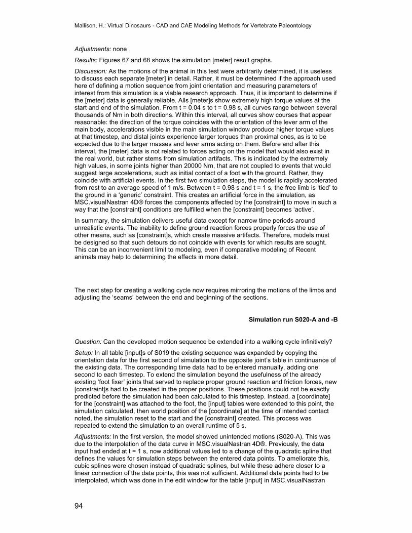
Mallison, H.: Virtual Dinosaurs - CAD and CAE Modeling Methods for Vertebrate Paleontology
94
Adjustments: none
Results: Figures 67 and 68 shows the simulation [meter] result graphs.
Discussion: As the motions of the animal in this test were arbitrarily determined, it is useless to discuss each separate [meter] in detail. Rather, it must be determined if the approach used here of defining a motion sequence from joint orientation and measuring parameters of interest from this simulation is a viable research approach. Thus, it is important to determine if the [meter] data is generally reliable. Alls [meter]s show extremely high torque values at the start and end of the simulation. From t = 0.04 s to t = 0.98 s, all curves range between several thousands of Nm in both directions. Within this interval, all curves show courses that appear reasonable: the direction of the torque coincides with the orientation of the lever arm of the main body, accelerations visible in the main simulation window produce higher torque values at that timestep, and distal joints experience larger torques than proximal ones, as is to be expected due to the larger masses and lever arms acting on them. Before and after this interval, the [meter] data is not related to forces acting on the model that would also exist in the real world, but rather stems from simulation artifacts. This is indicated by the extremely high values, in some joints higher than 20000 Nm, that are not coupled to events that would suggest large accelerations, such as initial contact of a foot with the ground. Rather, they coincide with artificial events. In the first two simulation steps, the model is rapidly accelerated from rest to an average speed of 1 m/s. Between t = 0.98 s and t = 1 s, the free limb is ‘tied’ to the ground in a ‘generic’ constraint. This creates an artificial force in the simulation, as MSC.visualNastran 4D® forces the components affected by the [constraint] to move in such a way that the [constraint] conditions are fulfilled when the [constraint] becomes ‘active’.
In summary, the simulation delivers useful data except for narrow time periods around unrealistic events. The inability to define ground reaction forces properly forces the use of other means, such as [constraint]s, which create massive artifacts. Therefore, models must be designed so that such detours do not coincide with events for which results are sought. This can be an inconvenient limit to modeling, even if comparative modeling of Recent animals may help to determining the effects in more detail.
The next step for creating a walking cycle now requires mirroring the motions of the limbs and adjusting the ‘seams’ between the end and beginning of the sections.
Simulation run S020-A and -B
Question: Can the developed motion sequence be extended into a walking cycle infinitively?
Setup: In all table [input]s of S019 the existing sequence was expanded by copying the orientation data for the first second of simulation to the opposite joint’s table in continuance of the existing data. The corresponding time data had to be entered manually, adding one second to each timestep. To extend the simulation beyond the usefulness of the already existing ‘foot fixer’ joints that served to replace proper ground reaction and friction forces, new [constraint]s had to be created in the proper positions. These positions could not be exactly predicted before the simulation had been calculated to this timestep. Instead, a [coordinate] for the [constraint] was attached to the foot, the [input] tables were extended to this point, the simulation calculated, then world position of the [coordinate] at the time of intended contact noted, the simulation reset to the start and the [constraint] created. This process was repeated to extend the simulation to an overall runtime of 5 s.
Adjustments: In the first version, the model showed unintended motions (S020-A). This was due to the interpolation of the data curve in MSC.visualNastran 4D®. Previously, the data input had ended at t = 1 s, now additional values led to a change of the quadratic spline that defines the values for simulation steps between the entered data points. To ameliorate this, cubic splines were chosen instead of quadratic splines, but while these adhere closer to a linear connection of the data points, this was not sufficient. Additional data points had to be interpolated, which was done in the edit window for the table [input] in MSC.visualNastran
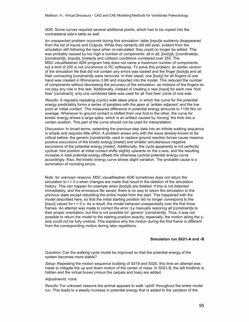
Mallison, H.: Virtual Dinosaurs - CAD and CAE Modeling Methods for Vertebrate Paleontology
95
4D®. Some curves required several additional points, which had to be copied into the contralateral side’s table as well.
An unexpected problem occurred during this simulation: table [input]s suddenly disappeared from the list of Inputs and Outputs. While they certainly did still exist, evident from the simulation still following the input when re-calculated, they could no longer be edited. This was probably caused by too high a number of components: all in all, [body]s, [coordinate]s, [constraint]s, [input]s, [meter]s and collision conditions numbered over 255. The MSC.visualNastran 4D® program help does not name a maximum number of components, but a limit of 255 is not uncommon in PC softwares. To solve this problem, an earlier version of the simulation file that did not contain any errors was loaded and the finger [body]s and all their connecting [constraint]s were removed. In their stead, one [body] for all fingers of one hand was created in Rhinoceros 3.0® and imported into the model. This reduced the number of components without decreasing the accuracy of the simulation, as motions of the fingers do not play any role in this test. Additionally, instead of creating a new [input] for each new ‘foot fixer’ [constraint], only one combined table was used for all ‘foot fixer’ joints of one side.
Results: A regularly repeating (cyclic) walk takes place, in which the curve for the potential energy predictably forms a series of parables with the apex at ‘ankles adjacent’ and the low point at ‘initial contact’. The measured difference in potential energy amounts to 1150 Nm on average. Whenever to ground contact is shifted from one foot to the other, the curve for kinetic energy shows a large spike, which is an artifact caused by ‘forcing’ the limb into a certain position. This part of the curve should not be used for interpretation.
Discussion: In broad terms, extending the previous step data into an infinite walking sequence is simple and requires little effort. A problem arises only with the issue already known to be critical before: the generic [constraint]s used to replace ground reaction forces cause massive positive excursions of the kinetic energy [meter] and smaller simultaneous negative excursions of the potential energy [meter]. Additionally, the cycle apparently is not perfectly cyclical: foot position at initial contact shifts slightly upwards on the z-axis, and the resulting increase in total potential energy offsets the otherwise cyclical potential energy curve accordingly. Also, the kinetic energy curve shows slight variation. The probable cause is a summation of rounding errors.
Note: for unknown reasons, MSC.visualNastran 4D® sometimes does not return the simulation to t = 0 s when changes are made that result in the deletion of the simulation history. This can happen for example when [body]s are deleted. If this is not detected immediately, and the erroneous file saved, there is no way to return the simulation to the previous state except rebuilding the entire model from the start. This happened with the model described here, so that the initial starting position did no longer correspond to the [input] values for t = 0 s. As a result, the model behaved unexpectedly over the first three frames. An attempt was made to correct the error, by manually restoring all [constraint]s to their proper orientation, but this is not possible for ‘generic’ [constraint]s. Thus, it was not possible to return the model to the starting position exactly; especially, the motion along the y-axis could not be fully undone. This explains why the motion during the first frame is different from the corresponding motion during later repetitions.
Simulation run S021-A and -B
Question: Can the walking cycle model be improved so that the potential energy of the system becomes more stable?
Setup: Repeating the motion sequence building of S019 and S020, this time an attempt was made to mitigate the up and down motion of the center of mass. In S021-B, the left hindlimb is hidden and the virtual bones (minus the carpals and toes) are added.
Adjustments: none
Results: For unknown reasons the animal appears to walk ‘uphill’ throughout the entire model run. This leads to a steady increase in potential energy that is added to the variation of the
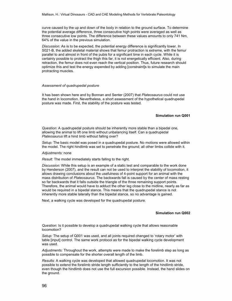
Mallison, H.: Virtual Dinosaurs - CAD and CAE Modeling Methods for Vertebrate Paleontology
96
curve caused by the up and down of the body in relation to the ground surface. To determine the potential average difference, three consecutive high points were averaged as well as three consecutive low points. The difference between these values amounts to only 741 Nm, 64% of the value in the previous simulation.
Discussion: As is to be expected, the potential energy difference is significantly lower. In S021-B, the added skeletal material shows that femur protraction is extreme, with the femur parallel to and almost in front of the pubis for a significant time in each cycle. While it is certainly possible to protract the thigh this far, it is not energetically efficient. Also, during retraction, the femur does not even reach the vertical position. Thus, future research should optimize this and test the energy expended by adding [constraint]s to simulate the main protracting muscles.
Assessment of quadrupedal posture
It has been shown here and by Bonnan and Senter (2007) that Plateosaurus could not use the hand in locomotion. Nevertheless, a short assessment of the hypothetical quadrupedal posture was made. First, the stability of the posture was tested.
Simulation run Q001
Question: A quadrupedal posture should be inherently more stable than a bipedal one, allowing the animal to lift one limb without unbalancing itself. Can a quadrupedal Plateosaurus lift a hind limb without falling over?
Setup: The basic model was posed in a quadrupedal posture. No motions were allowed within the model. The right hindlimb was set to penetrate the ground; all other limbs collide with it.
Adjustments: none
Result: The model immediately starts falling to the right.
Discussion: While this setup is an example of a static test and comparable to the work done by Henderson (2007), and the result can not be used to interpret the stability of locomotion, it allows drawing conclusions about the usefulness of 4-point support for an animal with the mass distribution of Plateosaurus. The backwards fall is caused by the center of mass resting so far backwards that it falls outside the triangle of the three remaining support points. Therefore, the animal would have to adduct the other leg close to the midline, nearly as far as would be required in a bipedal stance. This means that the quadrupedal stance is not inherently more stable laterally than the bipedal stance, so no advantage is gained.
Next, a walking cycle was developed for the quadrupedal posture.
Simulation run Q002
Question: Is it possible to develop a quadrupedal walking cycle that allows reasonable locomotion?
Setup: The setup of Q001 was used, and all joints required changed to ‘rotary motor’ with table [input] control. The same work protocol as for the bipedal walking cycle development was used.
Adjustments: Throughout the work, attempts were made to make the forelimb step as long as possible to compensate for the shorter overall length of the limb.
Results: A walking cycle was developed that allowed quadrupedal locomotion. It was not possible to extend the forelimb stride length sufficiently to the length of the hindlimb stride, even though the hindlimb does not use the full excursion possible. Instead, the hand slides on the ground.
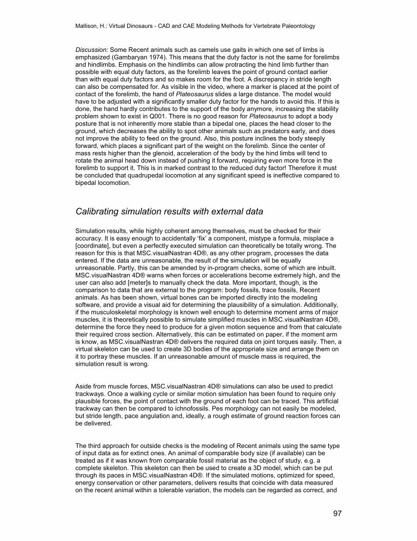
Mallison, H.: Virtual Dinosaurs - CAD and CAE Modeling Methods for Vertebrate Paleontology
97
Discussion: Some Recent animals such as camels use gaits in which one set of limbs is emphasized (Gambaryan 1974). This means that the duty factor is not the same for forelimbs and hindlimbs. Emphasis on the hindlimbs can allow protracting the hind limb further than possible with equal duty factors, as the forelimb leaves the point of ground contact earlier than with equal duty factors and so makes room for the foot. A discrepancy in stride length can also be compensated for. As visible in the video, where a marker is placed at the point of contact of the forelimb, the hand of Plateosaurus slides a large distance. The model would have to be adjusted with a significantly smaller duty factor for the hands to avoid this. If this is done, the hand hardly contributes to the support of the body anymore, increasing the stability problem shown to exist in Q001. There is no good reason for Plateosaurus to adopt a body posture that is not inherently more stable than a bipedal one, places the head closer to the ground, which decreases the ability to spot other animals such as predators early, and does not improve the ability to feed on the ground. Also, this posture inclines the body steeply forward, which places a significant part of the weight on the forelimb. Since the center of mass rests higher than the glenoid, acceleration of the body by the hind limbs will tend to rotate the animal head down instead of pushing it forward, requiring even more force in the forelimb to support it. This is in marked contrast to the reduced duty factor! Therefore it must be concluded that quadrupedal locomotion at any significant speed is ineffective compared to bipedal locomotion.
Calibrating simulation results with external data
Simulation results, while highly coherent among themselves, must be checked for their accuracy. It is easy enough to accidentally ‘fix’ a component, mistype a formula, misplace a [coordinate], but even a perfectly executed simulation can theoretically be totally wrong. The reason for this is that MSC.visualNastran 4D®, as any other program, processes the data entered. If the data are unreasonable, the result of the simulation will be equally unreasonable. Partly, this can be amended by in-program checks, some of which are inbuilt. MSC.visualNastran 4D® warns when forces or accelerations become extremely high, and the user can also add [meter]s to manually check the data. More important, though, is the comparison to data that are external to the program: body fossils, trace fossils, Recent animals. As has been shown, virtual bones can be imported directly into the modeling software, and provide a visual aid for determining the plausibility of a simulation. Additionally, if the musculoskeletal morphology is known well enough to determine moment arms of major muscles, it is theoretically possible to simulate simplified muscles in MSC.visualNastran 4D®, determine the force they need to produce for a given motion sequence and from that calculate their required cross section. Alternatively, this can be estimated on paper, if the moment arm is know, as MSC.visualNastran 4D® delivers the required data on joint torques easily. Then, a virtual skeleton can be used to create 3D bodies of the appropriate size and arrange them on it to portray these muscles. If an unreasonable amount of muscle mass is required, the simulation result is wrong.
Aside from muscle forces, MSC.visualNastran 4D® simulations can also be used to predict trackways. Once a walking cycle or similar motion simulation has been found to require only plausible forces, the point of contact with the ground of each foot can be traced. This artificial trackway can then be compared to ichnofossils. Pes morphology can not easily be modeled, but stride length, pace angulation and, ideally, a rough estimate of ground reaction forces can be delivered.
The third approach for outside checks is the modeling of Recent animals using the same type of input data as for extinct ones. An animal of comparable body size (if available) can be treated as if it was known from comparable fossil material as the object of study, e.g. a complete skeleton. This skeleton can then be used to create a 3D model, which can be put through its paces in MSC.visualNastran 4D®. If the simulated motions, optimized for speed, energy conservation or other parameters, delivers results that coincide with data measured on the recent animal within a tolerable variation, the models can be regarded as correct, and
Mallison, H.: Virtual Dinosaurs - CAD and CAE Modeling Methods for Vertebrate Paleontology
98
the same techniques used for extinct taxa. In this project, it was not possible to complete such a modeling of a Recent species due to time constraints, but a preliminary modeling attempt on Brachiosaurus brancai, in which not the orientation of the joints was dictated, but rather the applied torques, resulted in a tolt-like gait.
Simulation run S022
Elephants, morphologically extremely similar to large sauropods, are also dynamically similar, as they possess roughly similar strength indicators (Alexander 1989). The simulation aimed for any gait that allowed pes overprint of the manus in the trackway, as trackways with this characteristic are known from sauropods. By trial and error, various relative limbs positions resulting in various different gaits were tested. Intentionally, a high average speed of 18 km/h was chosen, as this is close to the hypothetical walk/trot transition for Brachiosaurus. Also, such a high speed is required to produce the overprint effect. In all, only one type of gait remained feasible, as it provided sufficient clearance between the limbs on one side so that the animal would not kick itself while at the same time providing maximum support. This gait is in horses often called a tolt or tölt, and is the same gait elephants use at medium to high speeds (Gambaryan 1974). While this is no proof of the correctness of the simulation, it is a strong indication that kinetic/dynamic modeling can be used for such research question.
Future Research
The most important aim for future research is the calibration of kinetic/dynamic modeling of extinct animals in NASTRAN-based software by applying the program and the methods developed here to Recent animals. Ideally, both graviportal (elephant) and large animals capable of high speed gaits (rhinoceros, Cape buffalo, giraffe, hippopotamus) as well as smaller and lighter animals, possibly various ungulates, should be investigated. Additionally, ostriches and other bipedal animals including kangaroos would make interesting subjects for modeling. With regards to extinct taxa, a broadening of the methodology is desirable. On one hand, the existing methods for developing walking cycles should be improved, allowing for more varied control and for automation of optimizing procedures. Trial&error procedures as employed here, while important to determine the main points of a problem quickly, require intuition and luck to deliver results, and can not be used to develop comparative modeling series of many taxa in a short time. Also, new solutions for the modeling of ground reaction forces are required. On the other hand, the existing techniques should be employed to a wider field of study with regards to motions: in addition to locomotion, attack and defense behavior such as the tail swinging of stegosaurs and ankylosaurs, the dorsal attack bite into hadrosaur hips by tyrannosaurs and similar issued could be investigated. What torque along the longitudinal axis does a Tyrannosaurus rex experience if it bites a large prey animal which runs on a perpendicular course? How large a prey animal can a tyrannosaurid dinosaur drag away? And how much weight can an Allosaurus move? What body motions can a large theropod employ to lower the damage from a fall at high running speed by reducing the impact force or shifting it to body parts that are less prone to receive lethal damage? Can the empirically determined results of Manning (2006), who claim that the dromaesaur’s enlarged digit was not a disemboweling weapon but a grappling hook, be reproduced in computer simulation? Alls these issues are potential applications for modeling in MSC.visualNastran 4D®.
Mallison, H.: Virtual Dinosaurs - CAD and CAE Modeling Methods for Vertebrate Paleontology
99
CONCLUSIONS SECTION III
Kinetic modeling with MSC.visualNastran 4D® has proven to be a helpful tool in vertebrate paleontology. Even though the program is limited to simulation rigid bodies, important insights into biomechanical issues can be gained by careful simulation setup. MSC.visualNastran 4D® is easy to use, requires no special knowledge of advanced mathematics and offers sufficient options for customizing models so that it can be easily employed for a wide variety of problems. The following topics can be easily investigated: position of the center of mass for uniform and varying densities, ranges of motion and the effect of motions on balance, locomotion cycles, required and experienced torques in joints during static and dynamic analysis, and both potential and kinetic energy levels during (loco-)motion.
At any time, simulation results can be checked against other data. From motion simulation, data on the arrangement of skeletal elements can be extracted and used to test, either with real or virtual bones or casts, whether the simulation would require disarticulation. Locomotion cycles allow the creation of artificial trackways, which can be compared to ichnofossils. While ground reaction forces are hard to define and compute, torques in individual joints can be determined and their probability tested by simplified musculoskeletal computer models or mathematical model calculations. Also, simulation of Recent animals compared to video data allows reliable calibration of the method.
Simulating Plateosaurus engelhardti in MSC.visualNastran 4D® shows clearly that the animal was capable of adopting a bipedal posture and walk in it, while quadrupedality can be ruled out due to the unstable nature of a quadrupedal stance. Even wide variations in overall body mass or mass distribution do not move the center of mass into a position that makes a bipedal stance improbable, much less impossible. This robustness also means that the differences in density between various tissue types can be ignored in prosauropods, as the error incurred is smaller than that incurred in soft tissue reconstruction. For a bipedal posture, the torque values in the major limb joints are shown to be in a reasonable range to be compensated passively by muscle and tendon stretching. Additionally, the models show that basic motions any animal must be able to perform also do not destabilize Plateosaurus easily if the limbs are placed reasonably: they were held nearly vertical in anterior aspect and showed the typical zigzag posture known from recent animals with functional three-part limbs. The thigh is protracted somewhat, so that the knee is positioned in font of the center of gravity, while the posteriorly inclined lower leg places the ankle just behind the center of mass. Finally, the models created can serve to assess the range of motion of Plateosaurus, by defining the maximum and minimum values of rotation in each joint according to values determined from the actual bones. Locomotion cycles can easily be developed in MSC.visualNastran 4D® and can be optimized and adapted for various research tasks.
IMPLICATIONS FOR THE AUTECOLOGY OF PLATEOSAURUS
The interpretations of the ecological role of Plateosaurus is somewhat influenced by the results of this study. In opposition to the recent trend to portray Plateosaurus as a quadruped, which makes locomotion the main use of the forelimbs, the bipedal posture raises the question why the arms are so sturdy and the vertebral column so resistant to bending moments in the pectoral region. This connection suggests that large forces were transmitted through the pectoral girdle, and in connection with the grasping ability of the hand and the strong development of solid, slightly curved claws it is possible to infer a number of different uses of the arms, all of them not mutually exclusive. The ability to grasp and powerfully hold things can be useful for acquiring food: ripping off tough branches of plants, scratching roots and subterranean shoots out of soft or hard sediments, or possibly just scratching a small depression, then grasping and ripping out the roots, or ripping large seeds or similar structures off a tough base (e.g. cycad seeds) all seem feasible. As shown by Senter (2005),
Mallison, H.: Virtual Dinosaurs - CAD and CAE Modeling Methods for Vertebrate Paleontology
100
possession of two or three claws as opposed to just one indicates the ability to break open hard sediments through powerful scratch-digging, while a single large claw is used like a crowbar on extremely hard substrates in so called hook-and-pull digging typical for anteaters or pangolins. The interpretation by Senter (2005) must however be treated with caution, as it is based on a small number of Recent animals to which the extinct taxa are compared. Plateosaurus reduces the fourth and fifth manual digit, but retains the first three with well developed interphalangal joints and strong, slightly curved claws. The attachment for the flexor muscles are strong, albeit much smaller than commonly seen in theropod dinosaurs or other predators or scavengers. This also means that the claws, while strong, do not indicate anything but a vegetarian diet for Plateosaurus, as is also indicated by the dentition (e.g. Huene 1932). The exclusively ventral reach of the arms limits this to objects in, on or near the ground, since it is not possible for the animal to bring the vertebral column into a near-upright position. Also, such motions would have to be carried out from side to side, as the only way to direct the tips of the claws to the ground is with fully extended wrists, which points the digits outwards at nearly 90°. While all this must remain speculation unless trace fossils of such scratching are found, one other possibility can be definitely excluded: Plateosaurus was not capable of breaking open extremely hard sediments, comparable e.g. to termite mounds.
The use of the forelimbs in intra- or interspecific combat by prosauropods as suggested by Bakker (1986, pers. comm. 2005) and Galton (1971, 1976) is unlikely. For one thing, it is near impossible to pose the animal in a way that allows the arms to reach another animal of similar size. Bonnan and Senter (2007) suggest interspecific grappling as in fighting male kangaroos (Dawson 1995) or precopulatory contest (Croft 1981), but this requires reaching so the arms face forward, not downward. Solely the grasping of the female by the male during copulation remains a possibility, similar to what has been suggested for Tyrannosaurus (Osborn 1916).
The locomotory capabilities of Plateosaurus have been underestimated by those advocating obligate quadrupedal locomotion. Since both energy efficient long distance walking with the limbs moving at their own pendulum frequency and rapid running are roughly proportional to limb length, shorter limbs mean slower speeds. In a quadruped, the limiting factor is the shorter limb pair. In Plateosaurus, the ratio between hindlimb and forelimb length is almost 1.9 (GPIT 1) or even higher (1.95 in AMNH 2409, Bonnan and Senter 2007), falling into the range of clearly bipedal theropods, which range from 1.49 to 4.80 according to Bonnan and Senter (2007). The hindlimb / trunk ratio, also invoked as indicating obligate quadrupedality in some prosauropods (e.g. Galton 1971, 1976), has been shown by Bonnan and Senter (2007) to be at best a parameter of questionable usefulness. Together with the elongation of the tibia, fibula and the metatarsals and the digitigrade stance, this indicates better cursorial adaptation than a hypothetical quadrupedal Plateosaurus would possess. Paul (1987) suggests, based on the view that all prosauropods were at most facultatively bipedal, that they retained a bounding gallop. As shown above, the plausible looking muscle reconstruction drawing shows an unrealistic pose and has scaling errors. Additionally, the fact that the humeri can not be protracted beyond vertical limits the forelimbs’ ability to cushion the impact of the bounding animal.
CONCLUSIONS
Studies in vertebrate paleontology can be greatly aided by the use of commercially available CAD (computer aided design) and NASTRAN-based CAE (computer aided engineering) softwares. They allow investigating various issues such as shapes, masses, position of the center of mass, balance and posture, range of motion and locomotion cycles easily, saving not only time on the necessary calculations but opening entirely novel approaches previously unthinkable of due to the sheer amount of data to be handled. The method developed here fall into three categories: first, the acquisition of digital data, creating virtual bones. These can replace the real fossils or casts of them in many investigations, are easy to handle, can be shared with researchers worldwide at low cost, and can find use in many applications. Most

Mallison, H.: Virtual Dinosaurs - CAD and CAE Modeling Methods for Vertebrate Paleontology
101
important of these is the creation of virtual dinosaur mounts and of rapid prototyped copies, both scaled and full size, for museum displays and research. The second category of methods and techniques relates to the reconstruction of extinct animals as 2D or 3D drawings or models. Comparison of the various techniques shows that 3D modeling on the basis of virtual skeletons can be the most exact method to create reconstructions and estimate mass, but requires careful consideration of soft tissues, as does as any other method.
The final tool investigated, kinetic/dynamic modeling with a rigid body motion analysis CAE program, shows how easily and quickly extinct animals can be posed and balanced in 3D, and how weight distribution and forces in the animals as well as their range of motion can be assessed. Motions and locomotion cycles can not only be animated, but also measured, and optimization, e.g. for minimal energy loss, is feasible.
Application of these methods to the prosauropod dinosaur Plateosaurus engelhardti MEYER
allowed the creation of an exact virtual skeleton, a highly detailed 3D model of the living animal, and a biomechanical assessment of the so far highly controversial issue of the posture and range of motion of this best-known large European dinosaur. Many previous reconstructions of Plateosaurus are inaccurate in many respects, especially overall proportions of the neck and limbs, as well as bone strength. It is shown here that Plateosaurus was an obligate biped, with medially directed palmar surfaces of the hands, and, while capable of a wide range of movements, was not able to walk quadrupedally. This provides a solid basis for a future investigation of the locomotory capabilities of Plateosaurus in comparison to ancestral and closely related taxa, which is of great interest as these large prosauropods possessed a locomotory grade only little removed from the common ancestor of all sauropodomorphs. Preliminary studies of locomotion cycles indicate that Plateosaurus was a capable cursor, able to move speedily. Expanding on this project, investigation of the early evolution of sauropodomorph locomotion with the tools developed here will allow new insights into the evolution of gigantism in sauropods.
Mallison, H.: Virtual Dinosaurs - CAD and CAE Modeling Methods for Vertebrate Paleontology
102
ACKNOWLEDGEMENTS First of all, my heartfelt thanks go to H.-U. Pfretzschner of the IFG, Tübingen University, who developed the idea for this project with me, supervised the work, guided me though it, taught me many an important fact or method and always had an open ear and a helpful comment on my work. A Doktorvater can not come any better.
When Prof. Pfretzschner was unable to continue supervising me, W.-E. Reif stepped in with excellent advice, enthusiasm and kind encouragement. He quickly became in integral part in shaping the direction of work and the final version of the thesis.
More aid from Tübingen came from the ever-helpful A. Hohloch, who patiently tested each and every new addition to the digitizing techniques I came up with. The work on digitizing bones was inspired by R. Wilhite, Louisiana State University School of Veterinary Medicine, who pioneered mechanical digitizing. In many discussions, he gave valuable advice and encouragement. Additional helpful discussions took place with K. Stevens of the University of Oregon Department of Computer and Information Science, N. Murphy of the Judith River Dinosaur Institute, A. Andersen of Virtual Surfaces Inc., and S. Hartmann from the Wyoming Dinosaur Center. A last-minute email exchange with S. Porchetti brought me up to date on the latest in prosauropod ichnology. S. Perry, Bonn University Institute for Zoology and J. Codd, University of Manchester Faculty of Life Sciences loaned me a longer-range Microscribe GL. I would like to extend my heartfelt appreciation to them all. W.-D. Heinrich, B. Schwarz, and S. Scheffler, all at the MNHB, Berlin, earned my gratefulness by helping with collection access. Equally deep in debt I am to C. and D. Mackie and especially K. Krudwig of RCI for access to the Berlin material in their care and many interesting discussions about the half-mounted skeletons of the MNHB.
For the mass estimate part of the work, the collaboration of E. Bachmann, Computational Science Department, Tübingen University, was invaluable. His plug-ins for Maya® made fast and easy 3D model creation possible, and he endured endless bickering about the tiniest inaccuracies with patience and good humor. T. Suthau, from the Remote Sensing Department of the Technical University Berlin, along with his colleagues and students, was a great help, both as a source of data and as someone to bounce ideas off. His boss, H.-C. Gunga, graciously allowed me the use of their data.
The computer modeling part of the thesis was greatly aided by T. Wolf, IZLBW, who came at an hours notice to get my PC back running whenever it broke down. C. Dechert, O. Wings and J. Hinz of the Institute of Geosciences, Tübingen University, were always willing to discuss the modeling.
Aside from those especially named already, all members of the Research Unit 533 have had a part in this work, most of all M. Sander, Institute for Paleontology, Bonn University, who took on the role of ‘replacement mentor’ when H.-U. Pfretzschner fell sick. Although he could not contribute much to the technical aspects of the work, his constant moral support, encouragement and urging me on has helped tremendously.
Last, but certainly far from least, my wife has helped me with her untiring support, especially during the stressful last few weeks of this work.
Mallison, H.: Virtual Dinosaurs - CAD and CAE Modeling Methods for Vertebrate Paleontology
LITERATURE CITED Ahlborn, B. K. 2004. Zoological Physics. Springer, Berlin. Alexander, R. M. 1976. Mechanics of bipedal locomotion. Pp. 493-504. In P. S. Davies, ed.
Perspectives in Experimental Biology. Vol. 1, Zoology. Proc. 50-th Anniversary Meeting Society of Experimental Biology.
Alexander, R. M. 1977. Mechanical scaling in terrestrial locomotion. In T. J. Padley, ed. Scale Effects in Animal Locomotion. Academic Press, London.
Alexander, R. M. 1985. Mechanics of posture and gait of some large dinosaurs. Zoological Journal of the Linnean Society 83(1):1-25.
Alexander, R. M. 1989. Dynamics of dinosaurs and other extinct giants.167. Alexander, R. M., and A. Vernon. 1975. The mechanics of hopping by kangaroos
(Macropodidae). Journal of Zoology, London 177:265-303. Anderson, J. F., A. Hall-Martin, and D. A. Russel. 1985. Long bone circumfence and weight in
mammals, birds and dinosaurs. Journal of Zoology 207:53-61. Aristotle. unknown. De motu animalium (on the movements of animals). Translation by
Farquharson, A. S. L. (2004) at http://etext.library.adelaide.edu.au/a/aristotle/gait/; The University of Adeleide Library.
Bachmann, E. 2006. Rekonstruktion und Animation eines Plateosaurus. Diploma Thesis, Eberhard-Karls-Universität Tübingen.
Bakker, B. 1986. Dinosaur Heresis. Kensington Publishing, New York. Bellmann, A., T. Suthau, S. Stoinski, A. Friedrich, O. Hellwich, and H.-C. Gunga. 2005. 3D-
Modelling of Dinosaurs. In Grün, and Kahmen, eds. Optical 3-D Measurement Techniques VII (Proceedings of the 7th Conference) Part 1. Vienna.
Blanco, E. R. 2003. Mechanical model for theoretical determination of maximum running speed in mammals. Journal of Theoretical Biology 222:117-125.
Blanco, E. R., and R. Gambini. 2006. A biomechanical model for size, speed and anatomical variations of the energetic costs of running mammals. Journal of Theoretical Biology 241:49-61.
Blanco, E. R., and G. Mazzetta. 2001. A new approach to evaluate the cursorial ability of the giant theropod Giganotosaurus carolinii. Acta Palaeontologica Polonica 46(2):193-202.
Bonaparte, J. F. 1971. Los tetrápodos del sector superior de la Formation Los Colorados, La Rioja, Argentina (Triásico Superior). Opera lilloana 22:1-183.
Bonnan, M. F. 2004. Morphometric analysis of humerus and femur shape in Morrison sauropods: implications for functional morphology and paleobiology. Paleobiology 30(3):444-470.
Bonnan, M. F., and P. Senter. 2007. Where the basal sauropodomorph dinosaurs Plateosaurus and Massospondylus habitual quadrupeds? In P. M. Barret, and D. J. Batten, eds. Evolution and palaeobiology of early sauropodomorph dinosaurs.
Bonnan, M. F., and A. M. Yates. 2007. A new description of the forelimb of the basal sauropodomorph Melanorosaurus: Implications for the evolution of pronation, manus shape and quadrupedalism in sauropod dinosaurs. In P. M. Barret, and D. J. Batten, eds. Evolution and palaeobiology of early sauropodomorph dinosaurs.
Bramwell, C. B., and G. R. Whitfield. 1974. Biomechanics of Pteranodon. Philosophical Transactions of the Rpyal Society of London, Series B 267:503-581.
Brilliant, K. 2002. Modeling Digital Dinosaurs. Charles River Media, Hingham, MA. Cavagna, G. A., N. C. Heglund, and C. R. Taylor. 1977. Mechanical work in terrestrial
locomotion: two basic mechanisms for minimizing energy expenditure. American Journal of Physiology 86:1657-1662.
Christian, A., and G. Dzemski. 2007. Reconstruction of the cervical skeleton posture of Brachiosaurus brancai Janensch, 1914 by an analysis of the intervertebral stress along the neck and a comparison with the results of different approaches. Fossil Record 10(1):38-49.
Christian, A., D. Koberg, and H. Preuschoft. 1996. Shape of the pelvis and posture of the hindlimbs in Plateosaurus. Palaeontologische Zeitschrift 70(3-4):591-601.
Christiansen, P. 1997. Locomotion in sauropod dinosaurs. Gaia 14:45-75.
Mallison, H.: Virtual Dinosaurs - CAD and CAE Modeling Methods for Vertebrate Paleontology
Christiansen, P. 2000. Dionsaur biomechanics. Pp. 64-77. In G. S. Paul, ed. The Scientific American Book of Dinosaurs. Byron Press, New York.
Christiansen, P., and R. A. Farina. 2004. Mass prediction in theropod dinosaurs. Journal of Paleobiology 16(2-4):85-92.
Colbert, E. H. 1962. The weights of dinosaurs. American Museum Novitates 2076:16. Daniels, C. B., and J. Pratt. 1992. Breathing in long necked dinosaurs: did sauropods have
bird lungs? Comparative Biochemistry and Physiology 101A(1):43-46. Dawson, T. J., and C. R. Taylor. 1973. Energetic cost of locomotion in kangaroos. Nature
390:67-70. Dzemski, G. 2006a. Funktionsmorphologische Analysen langer Hälse bei rezenten
terrestrischen Wirbeltieren zur Rekonstruktion der Stellung und Beweglichkeit langer Hälse prähistorischer Tiere. Doctoral Thesis, Universität Flensburg.
Dzemski, G. 2006b. Funktionsmorphologische Betrachtung der Halsstellung bei Zoogiraffen. Zoologischer Garten 75:189-201.
Ellenberger, P. 1972. Les niveaux paléontologiques de première apparition des Mammifères primordiaux en Afrique du Sud et leur Ichnologie etablissement de zones stratigraphiques detaillées dans le Stromberg du Lesotho (Afrique du Sud) (Trias supérieur à Jurassique). Second Gondwana Symposium South Africa, July to August 1970, Proceedings and Papers: 343-370:[publication date fide Bull. sign. (1972) 224, E, 33 (11-12), No 2430].
Farlow, J. O., M. B. Smith, and J. M. Robinson. 1995. Body mass, bone "strength indicator", and cursorial potential of Tyrannosaurus rex. Journal of Vertebrate Paleontology 15:713-752.
Fox, L. 1962. Numerical Solutions of Ordinary and Partial Differential Equations. Addison-Wesley, Palo Alto.
Fraas, E. 1912. Die schwäbischen Dinosaurier. Jahreshefte des Vereins für vaterländische Naturkunde in Württemberg 68:lxvi-lxvii.
Fraas, E. 1913. Die neuesten Dinosaurierfunde in der schwäbischen Trias. Naturwissenschaften 45:1097-1100.
Galton, P. M. 1971. The prosauropod Ammosaurus, the crocodile Protosuchus, and their bearing on the age of the Navajo Sandstone of northeastern Arizona. Journal of Plaeontology 45:781-795.
Galton, P. M. 1976. Prosauropod dinosaurs of North America. Postilla 169:1-98. Galton, P. M. 1985. Diet of prosauropod dinosaurs from the Late Triassic and Ealry
Jurassic. Lethaia 18(2):105-123. Galton, P. M. 1990. Basal sauropodomorpha - Prosauropod. In D. B. Weishampel, and H.
Osmólska, eds. The Dinosauria. University of California Press, Berkeley. Galton, P. M., and P. Upchurch. 2004. Prosauropods. Pp. 232-258. In D. B. Weishampel, P.
Dodson, and H. Osmólska, eds. The Dinosauria, 2nd edition. University of California Press, Berkeley.
Gambaryan, P. P. 1974. How Mammals Run. Keter Publishing House, Jerusalem. Golder, W., and A. Christian. 2002. Quantitative CT of dinosaur bone. Journal of Computer
Assisted Tomography 26(5):821-824. Goldfinger, E. 2004. Animal anatomy for the artist. Oxford University Press, Oxford. Goswami, A. 2004. Cranial modularity across mammalia: morphometric analysis of
phylogenetically and ecologically-related variation. Journal of Vertebrate Paleontology 24(Supplement to No. 3):65A.
Gould, G. C., L. F. Marcus, A. P. Gueziec, G. F. Daleo, and D. P. Reddy. 1996. Medical CT scan visualization and its application for the study of fossils using Data Explorer and InterFormat. Journal of Vertebrate Paleontology 16(Supplement to No. 3):38.
Gunga, H.-C., K. Kirsch, J. Rittweger, L. Röcker, A. Clarke, J. Albertz, A. Wiedemann, S. Mokry, T. Suthau, A. Wehr, W.-D. Heinrich, and H.-P. Schultze. 1999. Body Size and Body Volume Distribution in two Sauropods from the Upper Jurassic of Tendaguru (Tanzania). Mitt. Mus. Nat.kd Berl., Geowiss Reihe 2:91-102.
Gunga, H.-C., K. A. Kirsch, F. Baartz, L. Röcker, W.-D. Heinrich, W. Lisowski, A. Wiedemann, and J. Albertz. 1995. New data on the dimensions of Brachiosaurus brancai and their physiological implications. Naturwissenschaften 82(4):190-192.
Gunga, H.-C., T. Suthau, A. Bellmann, A. Friedrich, T. Schwanebeck, S. Stoinski, T. Trippel, K. Kirsch, and O. Hellwich. in press. Body mass estimations for Plateosaurus
Mallison, H.: Virtual Dinosaurs - CAD and CAE Modeling Methods for Vertebrate Paleontology
engelhardti using laser scanning and 3D reconstruction methods. Naturwissenschaften.
Henderson, D. M. 1999. Estimating the masses and centers of mass of extinct animals by 3-D mathematical slicing. Paleobiology 25(1):88-106.
Henderson, D. M. 2007. Burly gaits: centers of mass, stability, and the trackways of sauropod dinosaurs. Journal of Vertebrate Paleontology 26(4):907-921.
Hester, P., A. Heckert, R. Berkhoudt, and S. Mathias. 2004. 30,000 vertebrate fossils online: New Mexico Museum of Natural History and Science's digital database, a research tool. Journal of Vertebrate Paleontology 24(Supplement to No. 3):70A.
Hildebrand, M., and G. E. Goslow. 2003a. Analysis of Vertebrate Structure (international edition). Wiley-VCH, Berlin.
Hildebrand, M., and G. E. Goslow. 2003b. Vergleichende und funktionelle Anatomie der Wirbeltiere. Springer, Berlin.
Hitchcock, E. 1847. Description of two new species of fossil footmarks found in Massachusatts and Connecticut, or, of the animals that made them. American Journal of Sciences, Series 2 4:46-57.
Holliday, C. M., R. C. Ridgely, J. C. Sedlmayr, and L. M. Witmer. 2001a. The articular cartilage of extant archosaur limb bones: implications for dinosaur functional morphology and allometry. Jounral of Morphology 248(3):241-242.
Holliday, C. M., R. C. Ridgely, J. C. Sedlmayr, and L. M. Witmer. 2001b. The articular cartilage of extant archosaur limb bones: implications for dinosaur functional morphology and allometry. Journal of Vertebrate Paleontology 21(Supplement to No. 3).
Holliday, C. M., R. C. Ridgely, J. C. Sedlmayr, and L. M. Witmer. 2002. The articular cartilage of extant archosaur limb bones: implications for dinosaur functional morphology and allometry. Annual Meeting of the Society of Integratice and Comparative Biology, Anaheim, California. American Zoologist 416(6).
Huene, F. v. 1907-1908. Die Dinosaurier der europäischen Triasformation mit Berücksichtigung der aussereuropäischen Vorkomnisse. Geologische und paläontologische Abhandlungen Supplement-Band I:Text: xii + 419 S., 351 Abb; Atlas: Taf. - 1 Lief. (1907): 1-64, Abb. 1-47, Taf. 1-21; 2. Lief. (1908): 65-128, Abb. 48-124, Taf. 22-52; 3. Lief. (1908): 129-192, Abb. 125-205, Taf. 53-75; 4. Lief. (1908): 193-272, Abb. 206-279, Taf. 76-98; 5. Lief. (1908): 273-344, Abb. 280-321, Taf. 99-111; 6. Lief. (1908): i-xii + 345-419, Abb. 322-351.
Huene, F. v. 1926. Vollständige Osteologie eines Plateosauriden aus dem schwäbischen Keuper. Geologische und Palaeontologische Abhandlungen, Neue Folge 15(2):139-179.
Hutchinson, J. R. 2001a. The evolution of femoral osteology and soft tissues on the line to extant birds (Neornithes). Zoological Journal of the Linnean Society 131:169-197.
Hutchinson, J. R. 2001b. The evolution of pelvic osteology and soft tissues on the line to extant bords (Neornithes). Zoological Journal of the Linnean Society 131:123-168.
Hutchinson, J. R. 2003. The evolution of hindlimb tendons and muscles on the line to crown-group birds. Comparative Biochemistry and Physiology A 133:1051-1086.
Hutchinson, J. R., F. C. Anderson, S. S. Blemker, and S. L. Delp. 2005. Analysis of hindlimb muscle moment arms in Tyrannosaurus rex using a three-dimensional muscoloskeletal computer model: implications for stance, gait, and speed. Paleobiology 31(4):676-701.
Hutchinson, J. R., D. Farnini, R. Lair, and R. Kram. 2003. Are fast-moving elephants running? Nature 442:493-494.
Hutchinson, J. R., and S. M. Gatsey. 2000. Adductors, abductors, and the evolution of archosaur locomotion. Paleobiology 26:734-751.
Ikejiri, T. 2004. Relative growth and timing of ontogenetic changes in Camarasaurus (Dinosauria, Sauropoda). Journal of Vertebrate Paleontology 24(Supplement to No. 3):74.
Ikejiri, T., D. Schwarz, and B. Breithaupt. 2005. A nearly complete skeleton of a baby sauropod from the lower Morrison Formation of the Howe Stephens Quarry, Wyoming: "little steps" into diplodocid ontogeny and taxonomy. Journal of Vertebrate Paleontology 25(Supplement to No. 3):73A.
Jaekel, O. 1910. Die Fussstellung und Lebensweise der grossen Dinosaurier. Zeitschrift der Deutschen Geologischen Gesellschaft, Monatsberichte 62(4):270-277.
Mallison, H.: Virtual Dinosaurs - CAD and CAE Modeling Methods for Vertebrate Paleontology
Jaekel, O. 1911. Die Wirbeltiere. Eine Übersicht über die fossilen und lebenden Formen. Borntraeger, Berlin.
Knoll, F., E. Buffetaut, and M. Buelow. 1999. A theropod braincase from the Jurassic of the Vaches Noires cliffs (Normandy, France); osteology and palaeoneurology. Bulletin de la Societe Geologique de France 170(1):103-109.
Kummer, B. 2005. Biomechanik. Form und Funktion des Bewegungsapparats. Deutscher Ärzte-Verlag, Köln.
Kuznetsov, A. N. 1995. Energetical profit of the thrid segment in parasagittal legs. Journal of Theoretical Biology 172:95-105.
Lambert, D. 1980. A field guide to Dinosaurs. Avon Books, New York. Langer, M. C. 2003. The sacral and pelvic anatomy of the stem-sauropodomorph Saturnalia
tupiniquim (Late Triassic, Brazil). Paleobios 23(2):1-40. Leahy, G. 2003. Noses, lungs, and guts. Pp. 52-63. In G. S. Paul, ed. The Scientific American
Book of Dinosaurs. Byron Preiss, New York. Lockley, M., and C. Meyer. 2000. Dinosaur tracks and other fossil footprints of Europe.
Columbia University Press, New York. Manning, P. L., D. Payne, J. Pennicott, P. Barrett, and R. A. Ennos 2006. Dinosaur killer
claws or climbing crampons? Royal Society, Biology Letters 2(1):110-112 Marsh, O. C. 1893a. Restoration of Anchisaurus. American Journal of Science 45:169-170,
Taf. 6. Marsh, O. C. 1893b. Restoration of Anchisaurus, Ceratosaurus, and Claosaurus. Geological
Magazine 10(4):150-157. Mazzetta, G., and E. R. Blanco. 2001. Speeds of dinosaurs from the Albian–Cenomanian of
Patagonia and sauropod stance and gait. Acta Palaeontologica Polonica 46(2):235-246.
Mazzetta, G., P. Christiansen, and R. A. Farina. 2004. Giants and bizarres: Body size of some Southern South American Cretaceous dinosaurs. Historical Biology 16(2-4):1-13.
Meyer, H. v. 1837. [Brief an Prof. Bronn vom 4. April 1837]. Neues Jahrbuch für Mineralogie, Geognosie, Geologie un Petrefakten-Kinde 1837:314-316.
Moser, M. 2003. Plateosaurus engelhardti Meyer, 1837 (Dinosauria, Sauropodomorpha) aus dem Feuerletten (Mittelkeuper; Obertrias) von Bayern. Plateosaurus engelhardti Meyer, 1837 (Dinosauria, Sauropodomorpha) from the Feuerletten (middle Keuper, Upper Triassic) of Bavaria. Zitteliana. Reihe B, Abhandlungen der Bayerischen Staatssammlung fuer Palaeontologie und Geologie 24:186.
Motani, R. 2001. Estimating body mass from silhouettes: testing the assumption of elliptical body cross-sections. Paleobiology 27:735-750.
Muybridge, E. 1887. Animal Locomotion; An Electro-Photographic Investigation of Consecutive Phases of Animal Movement. Philadelphia.
Nicosia, U., and M. Loi. 2003. Triassic footprints from Lerici (La Spezia, Northern Italy). Ichnos 10:127-140.
Paul, G. S. 1987. The science and art of restoring the life appearance of dinosaurs and their relatives. A rigurous how-to guide. Pp. 4-49. In S. J. Czerkas, and E. C. Olson, eds. Dinosaurs Past and Present Vol. 2. University of Washington Press, Seattle.
Paul, G. S. 1988. The brachiosaur giants of the Morrison and Tendaguru with a description of a new subgenus, Giraffatitan, and a comparison of the world's largest dinosaurs. Hunteria 2(3):1-14.
Paul, G. S. 1996. The complete Illustrated Guide to Dinosaur Skeletons. Gakken Mook. Paul, G. S. 1997. Dinosaur models: the good, the bad, and using them to estimate the mass
of dinosaurs. Pp. 129-154. In D. L. Wolberg, E. Stump, and G. Rosenberg, eds. Dionfest International: Proceedings of a Symposium held at Arizona State University.
Paul, G. S. 2003. Restoring the life appearances of dinosaurs. Pp. 78-106. In G. S. Paul, ed. The Scientific American Book of Dinosaurs. Byron Preiss, New York.
Porchetti, S. D. O., and U. Nicosia. 2007. Re-examination of some large early mesozoic tetrapod footprints from the African collection of Paul Ellenberger. Ichnos 14(1-17).
Rainforth, E. C. 2003. Revision and re-evaluation of the Early Jurassic dinosaurian ichnogenus Otozoum. Palaeontology 46(4):803-838.
Reisz, R. R., D. Scott, H.-D. Sues, D. C. Evans, and M. A. Raath. 2005. Embryos of an early jurassic prosauropod dinosaur and their evolutionary significance. Science 309:761 - 764.
Mallison, H.: Virtual Dinosaurs - CAD and CAE Modeling Methods for Vertebrate Paleontology
Ridgely, R. C., and L. M. Witmer. 2004. New applications of CT scanning and 3D modeling for dinosaur visualization. Journal of Vertebrate Paleontology 24(Supplement to No. 3):103A-104A.
Ridgely, R. C., and L. M. Witmer. 2006. Dead on arrival: optimizing CT data acquisition of fossils using modern hospital CT scanners. Journal of Vertebrate Paleontology 26(Supplement to No. 3):115A.
Sander, P. M. 1992. The Norian Plateosaurus bonebeds of Central Europe and their taphonomy. Palaeogeography, Palaeoclimatology, Palaeoecology 93(3-4):255-299.
Sander, P. M., and N. Klein. 2005. Developmental plasticity in the life history of a prosauropod dinosaur. Science 310:1800-1802.
Schmidt-Nielsen, K. 1984. Scaling: Why is animal size so important? Cambridge University Press, Cambridge.
Schmidt-Nielsen, K. 1997. Animal Physiology: Adaptation and Environment. Cambirdge University Press, Cambridge.
Schwarz, D., E. Frey, and C. A. Meyer. 2006. Novel reconstruction of the orientation of the pectoral girdle in sauropods. Anatomical Record 290:32-47.
Schwarz, D., P. Vontobel, E. H. Lehman, C. A. Meyer, and G. Bongartz. 2005. Neutron tomography of internal sturctures of vertebrate remains: a comparison with X-ray computed tomography. Paleontologia Electronica 8(2):http://palaeo-electronica.org/2005_2/neutron/issue2_05.htm.
Seebacher, F. 2001. A new method to calculate allometric length-mass relationships of dinosaurs. Journal of Vertebrate Paleontology 21(1):51-60.
Senter, P. 2005. Function in the stunted forelimbs of Mononykus olecranus (Theropoda), a dinosaurian anteater. Paleobiology 31(3):373-381.
Stevens, K. A. 2002. DinoMorph: Parametric Modeling of skeletal structures. Senckenbergiana lethaea 82(1):23-34.
Stevens, K. A., and J. M. Parrish. 1996. Articulating three-dimensional computer models of sauropod cervical vertebrae. P. 67. In K. Padian, ed. Fifty-sixth annual meeting; Society of Vertebrate Paleontology; abstracts of papers. University of Oklahoma, Norman, OK, United States.
Stevens, K. A., and J. M. Parrish. 1997. Comparisons of neck form and function in the Diplodocidae. Journal of Vertebrate Paleontology 17(Supplement to No. 3):79A.
Stevens, K. A., and J. M. Parrish. 1999. Neck posture and feeding habits of two Jurassic sauropod dinosaurs. Science 284(5415):798-800.
Stevens, K. A., and J. M. Parrish. 2005. Neck posture, dentition, and feeding strategies in Jurassic sauropod dinsoaurs. Pp. 212-232. In V. Tidwell, and K. Carpenter, eds. Thunder-lizards: the sauropodomorph dinosaurs. Indiana University Press, Bloomington.
Stokstad, E. 2000. Learning to dissect dinosaurs, digitally. Science 288(5472):1728-1732. Sukhanov, V. B. 1967. Data on the locmotion of land vertebrates. 1. General classification of
symmetrical gaits. Byull. Mosk. Obshch. Ispyt. Prirody. Otd. Biol. 62(2):118-135 (Russian).
Sullivan, C., F. A. Jenkins, S. M. Gatsey, and n. H. Shubin. 2003. A functional assessment of the foot structure in the prosauropod dinosaur Plateosaurus. Journal of Vertebrate Paleontology 23:102A.
Suthau, T., A. Bellmann, F. Stoinski, A. Friedrich, O. Hellwich, and H.-C. Gunga. 2005. 3D- Rekonstruktion von Dinosauriern. P. 244. In T. Luhmann, ed. Photogrammetrie, Laserscanning, Optische 3D Messtechnik – Beiträge der Oldenburger 3D-Tage. Herbert Wichmann Verlag, Heidelberg.
Taylor, C. R., N. C. Heglund, and G. M. O. Maloiy. 1982. Energetics and mechanics of terrestrial locomotion. I. Metabolic energy consumption as a function of speed and body size in birds and mammals. Journal of Experimental Biology 97:1-21.
Van Heerden, J. 1997. Prosauropods. Pp. 242-263. In O. Farlow, and M. K. Brett-Surnam, eds. The Complete Dinosaur. Indiana University Press, Bloomington.
Vogel, S. 2003. Comparative Biomechanics. Princton University Press. von Huene, F. 1932. Die fossile Reptil-Ordnung Saurischia, ihre Entwicklung und Geschichte.
Monographien zur Geologie und Palaeontologie 1(4):361. Wedel, M. J. 2003a. The evolution of vertebral pneumaticity in sauropod dinosaurs. Journal of
Vertebrate Paleontology 23(2):344-357.
Mallison, H.: Virtual Dinosaurs - CAD and CAE Modeling Methods for Vertebrate Paleontology
Wedel, M. J. 2003b. Vertebral pneumaticity, air sacs, and the physiology of sauropod dinosaurs. Paleobiology 29(2):243-255.
Wedel, M. J. 2005. Postcranial skeletal pneumaticity in sauropods and its implications for mass estimates. Pp. 201-228. In J. A. Wilson, and K. Curry-Rodger, eds. The Sauropods: Evolution and Paleobiology. University of California Press, Berkeley.
Wedel, M. J. 2007. What pneumaticity tells us about 'prosauropods', and vice versa. Pp. 207-222. In P. M. Barret, and D. J. Batten, eds. Evolution and palaeobiology of early sauropodomorph dinosaurs.
Weishampel, D. B., and F. Westphal. 1986. Die Plateosaurier von Trossingen im Geologischen Institut der Eberhard-Karls-Universität Tübingen. Ausstellungskataloge der Universität Tübingen 19(1-27).
Wellnhofer, P. 1994. Prosauropod dinosaurs from the Feuerletten (Middle Norian) of Ellingen near Weissenburg in Bavaria. Revue de Paléobiologie Vol. spéc. 7 (1993):263-271.
Whittle, M. W. 1996. Gait analysis: an introduction. Butterworth Heinemann, Edinburgh. Wilhite, R. 2003a. Biomechanical reconstruction of the appendicular skeleton in three North
American Jurassic sauropods. Wilhite, R. 2003b. Digitizing large fossil skeletal elements for three-dimensional applications.
Paleontologia Electronica 5(2):http://palaeo-electronica.org/2002_2/scan/issue2_02.htm.
Yates, A. M. 2003. The species taxonomy of the sauropodomorph dinosaurs from the Lowenstein Formation (Norian, Late Triassic) of Germany. Palaeontology 46(2):317-337.
Yates, A. M., and C. C. Vasconcelos. 2003. Furcula-like clavicles in the prosauropod dinosaur Massospondylus. Journal of Vertebrate Paleontology 25(2):466-468.
Zuo, O., and W. Jing. 1995. First report on studying dinosaur egg fossils with method of medical CT scanning. Gushengwu Xuebao = Acta Palaeontologica Sinica 34(6):777-779.
Mallison, H.: Virtual Dinosaurs - CAD and CAE Modeling Methods for Vertebrate Paleontology
APPENDICES
Appendix A - Guide to digitizing and model creation techniques for Rhinoceros 3.0®
Abbreviations used herein: TIP – tip of the digitizer arm RFP – right foot pedal LFP – left foot pedal If asked to ‘at the command line enter…’, ensure that Rhinoceros 3.0® is ready for a new command (not already processing a command) and type the exact phrase given, then press the ENTER or RETURN key on the keyboard. ‘Select’ means click the appropriate box with the mouse so that a tick appears in the box, ‘deselect’ means to click the box so there is no tick in it. ‘Menu:’ refers to the pull-down menus at the top of the Rhinoceros 3.0® screen. Select the menu title given, and then select the (sub-)entry/-ies) given after the arrow(s) -->. For most commands, icons are available in Rhinoceros 3.0®. In the standard workplace setup, only a few are visible. These are referred to in the text. To make others available, refer to the in-program help. Commands need not be capitalized in Rhino, thus ‘points’ and ‘Points’ are equivalent. Note for users of earlier versions of Rhinoceros than 3.0 SR4: As opposed to Rhinoceros 3.0®, earlier versions do not automatically repeat the ‘digsketch’ command. It is necessary, after digitizing a curve or point(s), to press the left foot pedal (LFP) once to repeat the command. Also, any version before Service Release 4 (SR4) will not support polygon mesh creation via the ‘meshfrompoints’ command.
Digitizing preparations
To begin digitizing it is recommended to open a new file via the ‘New’ icon. This displays a selection of template files with varying units. For this study, the ‘centimeters.3dm’ template was used for all objects. This sets the scale of the coordinate axes as centimeters. Digitizing distance for curves should be selected accordingly. Open the file properties page (Menu: File --> Properties), select ‘Units’ and set the tolerances to values suitable for the task. Example values: Absolute tolerance: 0.01 units (0.001 for small bones) Relative tolerance: 0.1 percent Angle tolerance: 0.1 degree Tolerances should be at least an order of magnitude higher than the smallest value used in any operation on the data. Joining surfaces, e.g., requires distances smaller than 0.01 mm as the surfaces themselves are a theoretical 0.01 mm thick. Thus, absolute tolerance should be set to 0.001 mm. Angle tolerance should be equally low, as joining lines between surfaces otherwise will show as kinks.
Digitizing coordinates, (re-)calibration with and without moving the digitizer or specimen Initial setup and initial calibration: 1. Place the digitizer so it can reach all three coordinates marked on the specimen. 2. Connect the digitizer to Rhinoceros 3.0® (Menu: Tools --> 3-D Digitizer --> Connect, or enter ‘digcalibrate’ in the command line), select Digitizer type (Rhinoceros 3.0® suggests the Faro Digitizer; if using a different one, press ‘f’ and RETURN, then the first letter for your type of digitizer, confirm selections with RETURN). 3. When asked to ‘Enter origin with digitizer’ in the command line, place the tip of the digitizer (TIP) on the mark for the origin (O1) on the specimen and press the right foot pedal (RFP). 4. When asked to ‘Enter X-Axis with digitizer’ in the command line, place TIP on the mark for the origin (X1) on the specimen and press RFP. 5. When asked to ‘Enter Y-Axis with digitizer’ in the command line, place TIP on the mark for the origin (Y1) on the specimen and press RFP. 6. When asked to ‘Enter origin in Rhinoceros 3.0® (…)’, press RETURN
Mallison, H.: Virtual Dinosaurs - CAD and CAE Modeling Methods for Vertebrate Paleontology
Now the digitizer is ready for digitizing curves or points. The origin of the displayed coordinate system in Rhinoceros 3.0® coincides with O1 on the bone; the X-axis and Y-axis in Rhinoceros 3.0® run in the direction of X1 and Y1 respectively. Recalibration: To calibrate the digitizer back to the Cset1 (O1,X1,Y1) proceed as follows: 1. In the command line, enter ‘digcalibrate’ or choose ‘Menu: Tools --> 3-D Digitizer --> Calibrate’ 2. Proceed as above, starting with step 3. The digitizer is now recalibrated to the original coordinate set Cset1. Using several sets of coordinates: When using several sets of coordinates, it is important to mark each set on the bone as well as in Rhinoceros 3.0® so as to avoid mixing them up. In Rhinoceros 3.0® the author found it easiest not to add text or change object names but connect each set with a polyline and change the color of each X point. X1 was left unchanged (black), X2 changed to white, X3 to red etc., following the order of colors in Rhinoceros 3.0® layers. If this simple convention is kept, recalibration takes less time than with any other method while mix-ups can be avoided. In order to use several sets, mark all sets on the bone, calibrate the digitizer to Cset1 as above, and then proceed as follows: 1. In the command line, enter ‘points’. 2. Place the TIP on O2, press and release RFP. Watch the screen to note where the point appears. If necessary, shift the view using the ‘pan’ tool. 3. Repeat 2. to digitize X2 and Y2, note where they are on the screen. Press ESC after digitizing Y2. 4. At the command line enter ‘Polyline’. 5. On the screen, with the mouse select X2, O2, and Y2 in this order, press ENTER. To facilitate this, make sure that ‘OSnap’ is on and set to ‘Points’. See Rhinoceros 3.0® help for the use of ‘OSnap’. A polyline will appear with O2 at the meeting point of the two sections. 6. On the screen, select X2 (make sure the other points are deselected), press F3 and change the color of X2. 7. Repeat 2. to 6. until all sets have been digitized. To calibrate the digitizer to a different set (e.g., set 2), make sure the second set of coordinates has been digitized as points as described above. Place the digitizer so it can reach all three point of the set to calibrate to and proceed as follows: 1. At the command line enter ‘digcalibrate’ 2. When asked to ‘Enter origin with digitizer’ in the command line, place the tip of the digitizer (TIP) on the mark for the origin (O2) of this set on the specimen and press the right foot pedal (RFP). 3. When asked to ‘Enter X-Axis with digitizer’ in the command line, place TIP on the mark for the origin (X2) on the specimen and press RFP. 4. When asked to ‘Enter Y-Axis with digitizer’ in the command line, place TIP on the mark for the origin (Y2) on the specimen and press RFP. 5. When asked to ‘Enter origin in Rhinoceros 3.0® (…)’, use the mouse to select O2 in Rhinoceros 3.0®. To facilitate this, check that ‘Osnap (points)’ is on. 6. When asked to ‘Enter X-Axis in Rhinoceros 3.0® (…)’, use the mouse to select X2 in Rhinoceros 3.0®. 7. When asked to ‘Enter Y-axis in Rhinoceros 3.0® (…)’, use the mouse to select Y2 in Rhinoceros 3.0®. The digitizer is now calibrated to Cset2.
Digitizing and editing curves, points and pointclouds
Neighboring curves must be of similar length and should be roughly parallel. Large differences in length or distance produce artifacts. Also, curves may not cross each other. See Figure 7 for examples of well and badly placed curves. Digitizing points: The digitizer must be properly connected and calibrated before data can be gathered. 1. At the command line enter ‘points’ or click the appropriate icon in the 3d digitizing toolbar. 2. Place TIP at the desired location for the point and press RFP 3. To digitize more than one point, repeat 2.
Mallison, H.: Virtual Dinosaurs - CAD and CAE Modeling Methods for Vertebrate Paleontology
4. To end data collection, press ‘Esc’. Digitizing point clouds: A point cloud is a group of points that can be digitized in one continuous motion and is automatically grouped in Rhinoceros 3.0®. Ungrouping works best via the ‘explode’ command. The digitizer must be properly connected and calibrated before data can be gathered. 1. At the command line enter ‘pointcloud’ or click the appropriate icon in the 3d digitizing toolbar. It is also possible to enter ‘digsketch’ and select the appropriate options. 2. Place TIP at the desired location for the point and press and keep pressed RFP. 3. Move TIP across area for which points are to be digitized. 4. Release RFP to end point data collection. 5. To digitize more than one point cloud, repeat 2. to 4. 6. To end data collection, press ‘Esc’. Digitizing open curves: The digitizer must be properly connected and calibrated before data can be gathered. 1. At the command line enter ‘digsketch’ or select ‘Menu: Tool --> 3D Digitizer --> Sketch Curve’. 2. In the command line deselect ‘Points’ by pressing ‘p’ followed by ENTER and similarly select ‘Curves’ and deselect ‘Closed Curves’. Choose the distance at which points are to be placed on the curves by Rhinoceros 3.0®. Note that this distance depends on the scale of the template file you chose! Usually, 0.1 to 0.7 proved to be acceptable values, for very large objects with hardly any sudden curvature changes even a value of 1 is acceptable (using the centimeter template; change value accordingly if using other templates). Enter the value by changing the ‘Point Spacing’ value. 3. Place TIP at the desired starting location for the curve and press and keep pressed RFP. 4. Move TIP along the intended path of the curve 5. When TIP has reached the end location release RFP. 6. To digitize more than one closed curve repeat 3. to 5. 7. To end data collection, press ‘Esc’. Digitizing closed curves: The digitizer must be properly connected and calibrated before data can be gathered. 1. At the command line enter ‘digsketch’ or select ‘Menu: Tool --> 3D Digitizer --> Sketch Curve’. 2. In the command line deselect ‘Points’ by pressing ‘p’ followed by ENTER and similarly select ‘Curves’ and select ‘Closed Curves’. Choose the distance at which points are to be placed on the curves by Rhinoceros 3.0®. Note that this distance depends on the scale of the template file you chose! Usually, 0.1 to 0.7 proved to be acceptable values, for very large objects with hardly any sudden curvature changes even a value of 1 is acceptable (using the centimeter template; change value accordingly if using other templates). Enter the value by changing the ‘Point Spacing’ value. 3. Place TIP at the desired starting location for the curve (a point on the seam line) and press and keep pressed RFP. 4. Move TIP along the intended path of the curve 5. When TIP has almost reached the starting location again (1 to 2 mm gap) release RFP. 6. To digitize more than one closed curve repeat 3. to 5. 7. To end data collection, press ‘Esc’. Note: A small gap should be left between the start and end of a curve to guarantee a smooth connection at the seam. Failure to do so can lead to overlap, which produces artifacts on the lofted surface. Also, the start and end points should not show shift along the seam line, as this also leads to artifacts (Figure 14). Editing kinks and artifacts out of curves: This option should be used sparingly and can produce massive artifacts! 1. Rotate a viewport so that the view plane is as parallel to the main orientation of the curve as possible. This means that the curve ideally will lie flat on the viewplane. 2. At the command prompt enter ‘CPlanetoView’ to make the construction plane parallel with your view. 3. Select the curve to edit 4. Turn edit points on by clicking the icon at the lower left in the toolbar 5. Carefully select points and drag them to adjust the curve. Watch the changes in several viewports with different directions to avoid introducing deformations in the third axis. Rebuilding curves: Especially curves closed using the ‘match’ command have a very uneven distribution of their edit points. This tends to produce artifacts on lofts using these curves. In order to equally distribute the points on a curve the ‘rebuild’ command can be used. 1. At the command line enter ‘rebuild’ 2. Select the curve you want to rebuild. If several curves are to be rebuilt to the same standards (same number of points), these curves can be selected at the same time.
Mallison, H.: Virtual Dinosaurs - CAD and CAE Modeling Methods for Vertebrate Paleontology
3. Select the appropriate options. Usually, the same number of points that the curve already possesses should be chosen. 4. To rebuild more than one curve, repeat 1. to 3. Joining open curves into closed curves: Make sure the curves ends are close to each other. To ‘match’ several curves sets, always select the first and second curve in the same order to achieve equally directed closed curves with seam points aligned in one row. 1. At the command line enter ‘match’ 2. Select the first curve near the end that is supposed to be connected to the other curve. If only one of the curves is to be adjusted by Rhino, curve 1 must be the one that stays unchanged. 3. Select the second curve near the end that is supposed to be matched to the first curve. If only one of the curves is to be adjusted by Rhino, curve 2 must be the one that gets changed. 4. In the match dialog box, select the appropriate options. We recommend selecting ‘curvature’, ‘average curve’ and deselect ‘join’. ‘average curve’ adjusts both curves instead of only curve 2, leading to the distortion being more spread out but lesser in degree, reducing artifacts. 5. Repeat this process until both all contact points have been matched. 6. At the command line, enter ‘join’, then select the curves near the contact point. Note: In Rhinoceros 2.0®, it is possible to use the ‘join’ option in the ‘match’ options dialog. This does not work for Rhinoceros 3.0® as the curve can only be joined in one place with this option.
Lofting surfaces (open and closed) A flat surface resembles a sheet of paper, a closed surface open at the ends is a tube and a closed surface with closed ends results in a 3D body. It may be necessary to lower tolerances in the file properties to shorten computing time for lofting. Usually, this will not significantly reduce the accuracy of the lofted surface. Selecting curves automatically and manually for a loft (for all lofting options): Rhinoceros 3.0® usually sorts curves into the proper order when a group of curves is selected at the same time (automatic selection). This can be done by dragging a box over the curves with the mouse. Dragging from left to right will select only those curves that are completely within the dragged box, dragging from right to left will select all curves that are entirely or partially in the box. Rhinoceros 3.0® will also attempt to sort curve directions and adjust the seam line. Remember to de-select all other elements such as coordinates. If the loft contains both curves and points (start and end of closed lofts), the automatic sorting will usually fail. If automatic sorting does not work (i.e., the resulting surface curves back onto itself or shows other defects), curves must be selected manually. Here, the potential for mistakes is quite large, and care must be given to the following points. - All curves must be clicked with the mouse at the same end. Otherwise Rhinoceros 3.0® will attempt to form a surface that connects two opposite ends. - All curves must have the same direction (must have been digitized or later edited to have the same direction) - Curves must be selected one by one from one end of the bone to the other, otherwise the surface will fold back onto itself - For closed lofts, the end points must be selected first and last, with the curves in between in proper order. Lofting a flat surface: An open, flat loft requires as a minimum two curves. 1. At the command line enter ‘Loft’ 2. Select the appropriate curves 3. Press ENTER 4. Select the lofting options desired in the options box (see below) 5. Press ENTER 6. Click ‘Shade all viewports’ and check the surface for accuracy. Lofting a closed surface open at one or both ends: A closed surface requires closed curves. If an end is supposed to be closed, a point is required at that end. This method lets Rhinoceros 3.0® automatically adjust the seam points and directions of the curves; if the curves were digitized as advised above this should be free of problems. 1. At the command line enter ‘Loft’ 2. Select the appropriate curves and endpoint (if appropriate) 3. Press ENTER 4. Check that the selected curves all have the same direction (arrow at seam line); switch directions of odd curves
Mallison, H.: Virtual Dinosaurs - CAD and CAE Modeling Methods for Vertebrate Paleontology
5. Select the lofting options desired in the options box (see below) 6. Press ENTER 7. Click ‘Shade all viewports’ and check the surface for accuracy. Lofting a body (a closed surface closed at both ends): A closed surface requires closed curves. A point is required at each end. This method lets Rhinoceros 3.0® automatically adjust the seam points and directions of the curves; if the curves were digitized as advised above this should be free of problems. 1. At the command line enter ‘Loft’ 2. Select the appropriate curves and both endpoints, starting with one endpoints, then the curves in correct order, and the second endpoint last. 3. Press ENTER 4. Check that the selected curves all have the same direction (arrow at seam line); switch directions of odd curves 5. Select the lofting options desired in the options box (see below) 6. Press ENTER 7. Click ‘Shade all viewports’ and check the surface for accuracy. 8. Select ‘Analyze --> Mass Properties --> Volume’ and compare the given volume with a rough estimate to ensure that the loft actually resulted in the correct 3D body. Sometimes, the body will be open at some point and the surface folded back unto itself – the 3D body is hollowed out; this will result in a minuscule volume! Using the various ‘Loft’ options: A variety of options is available in the loft dialog box: For ‘Style’, there are: Normal - Uses chord-length parameterization in the loft direction. This is usually the best option to choose. Loose - results in a smother surface, but allows the surface to move away from the curves. This option should be used as rarely as possible, as it will significantly change the external appearance of smaller bones. Tight - Uses square root of chord-length parameterization in the loft direction which results in the surface sticking closely to the curves. This option tends to result in sharp changes of direction near the articular ends of bones. For ‘Simplify’, there are: Do not simplify - preferred option. Rebuild with control points - Rebuilds the shape curves before lofting. This is especially helpful if the curves change direction in small intervals a lot which can produce artifacts. Refit within units - Refits the shape curves to a tolerance value before lofting. Use same as the previous option. Troubleshooting: If the surface does not look correct, check the following: - Have all curves necessary been selected? Have all necessary end points been selected? If not, delete the surface and loft again. - Do all curves have the same direction? If not, delete the surface and loft again and change the directions. - Does any one curve show excessive differences from its neighbors (erroneous curve)? If so, delete the surface and loft again without the troublesome curve. - Do all curves look OK but the surface has odd wrinkles and twists? If so, delete the surface and try various ‘Simplify’ options of the loft dialog in a new loft. Or try rebuilding curves near the artifacts of the surface, and then loft again.
Editing and joining surfaces and bodies Some helpful Rhinoceros 3.0® commands are described here - for a tutorial on editing and combining surfaces please refer to the in-program help. Joining bodies smoothly in Rhinoceros 3.0® can be difficult, so the author advises against using multiple bodies whenever possible. Check that the tolerance levels are set to suitable values. Joining two bodies: 1. At the command line enter ‘BooleanUnion’ or select the icon from the toolbar at the left of the screen. 2. Select both bodies 3. Press ENTER Subtracting one body from another:
Mallison, H.: Virtual Dinosaurs - CAD and CAE Modeling Methods for Vertebrate Paleontology
1. At the command line enter ‘BooleanDifference’ or select the icon from the toolbar at the left of the screen (right-click BooleanUnion and select the second icon in the pop-up box) 2. Select the body from which to subtract the other body and press ENTER 3. Select the body to subtract and press ENTER. Intersecting two bodies: results in only the overlap being preserved. 1. At the command line enter ‘BooleanIntersection’ or select the icon from the toolbar at the left of the screen (right-click BooleanUnion and select the third icon in the pop-up box) 2. Select the bodies to intersect and press ENTER Creating a surface from a curve: 1. Select the curve 2. At the command line enter ‘patch’ and press enter. 3. As trimmed surfaces cannot by joined and tend to be difficult to use for cutting both surfaces and bodies we recommend to deselect ‘trim automatically’ in the dialog box. 4. Click OK. Using a surface as a cutting object to trim surfaces or bodies: 1. At the command line enter ‘Split’ (keeps the cut of pieces as separate objects) or ‘Trim’ (deletes the cut off pieces). 2. Select the object to split/trim. If trimming, click the part that should remain. 3. Select the cutting/trimming object. 4. Press ENTER. Creating a curve on a surface (for 3D model creation, can also be used as a cutting object) 1. Select the surface. 2. Select ‘Curve-->Free-Form-->Interpolate on Surface’. 3. Click on the surface at the start of the curve. 4. Click close to this first point in order to get tight control of the direction of the curve start. 5. Add more points to describe the surface. 6. Place the last clicks near each other to control the curvature exactly at the end of the curve. 7. Press ENTER.
Appendix B - Guide to point cloud and polygon mesh editing in Geomagic Qualify® 8.0 Note: Many actions are not reversible in Geomagic Qualify 8.0®, or only until the next action has been completed. Take care to save your data often and with altered filenames!
Creating polygon meshes from point clouds 1. Load the point cloud file. Acceptable formats are e.g. *.obj and *.igs 2. Choose a selection tool (‘Edit-->Selection Tools-->) and select erroneous points. 3. Delete selected points by pressing [Del]. Unmark the selection by pressing [Ctrl]+[C]. 4. Select the wrapping tool (‘Points-->Wrap’) and choose the ‘Surface’ wrap type. 5. Click ‘OK’
Removing artifacts from and smoothing a polygon mesh Smoothing cleans up the surface in one work step. Less aggressive are ‘Remove Noise’ and ‘Remove Spikes’. They allow the user to control the degree of smoothing, and ‘Remove Noise’ also has options to show the deviation between the original and the smoothed version. Smoothing a polygon mesh: 1. Select ‘Polygons-->Smooth’. 2. Click ‘OK’.
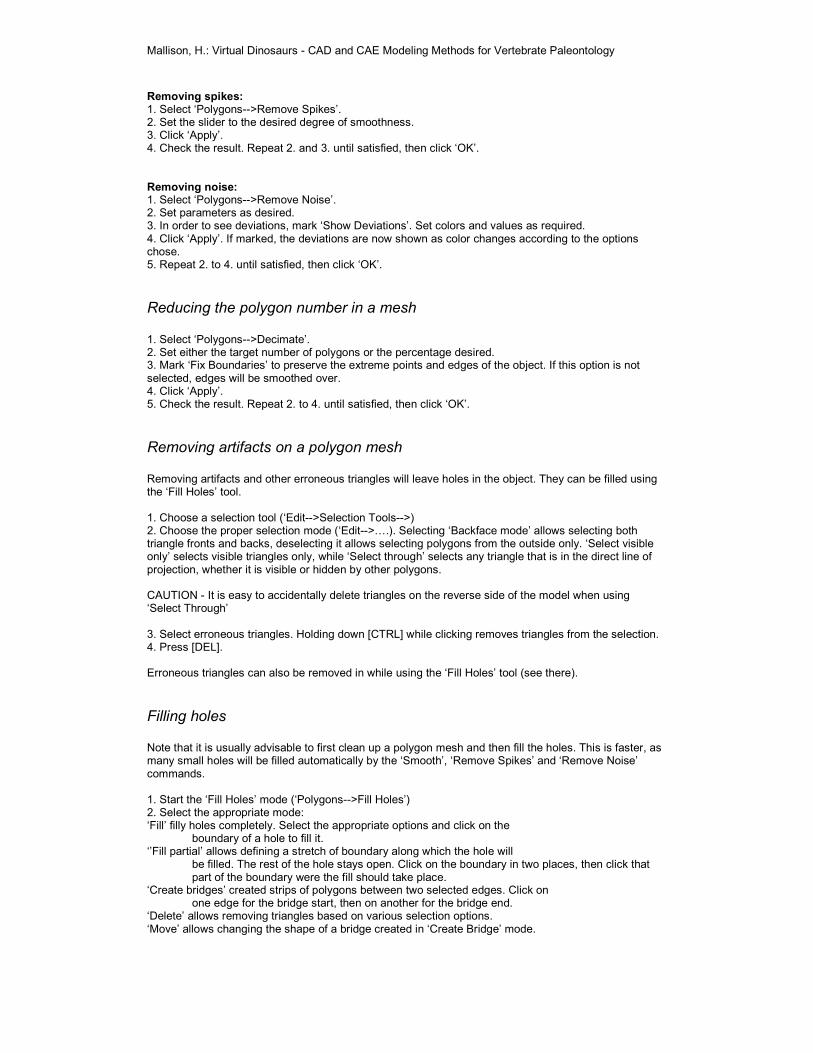
Mallison, H.: Virtual Dinosaurs - CAD and CAE Modeling Methods for Vertebrate Paleontology
Removing spikes: 1. Select ‘Polygons-->Remove Spikes’. 2. Set the slider to the desired degree of smoothness. 3. Click ‘Apply’. 4. Check the result. Repeat 2. and 3. until satisfied, then click ‘OK’. Removing noise: 1. Select ‘Polygons-->Remove Noise’. 2. Set parameters as desired. 3. In order to see deviations, mark ‘Show Deviations’. Set colors and values as required. 4. Click ‘Apply’. If marked, the deviations are now shown as color changes according to the options chose. 5. Repeat 2. to 4. until satisfied, then click ‘OK’.
Reducing the polygon number in a mesh 1. Select ‘Polygons-->Decimate’. 2. Set either the target number of polygons or the percentage desired. 3. Mark ‘Fix Boundaries’ to preserve the extreme points and edges of the object. If this option is not selected, edges will be smoothed over. 4. Click ‘Apply’. 5. Check the result. Repeat 2. to 4. until satisfied, then click ‘OK’.
Removing artifacts on a polygon mesh Removing artifacts and other erroneous triangles will leave holes in the object. They can be filled using the ‘Fill Holes’ tool. 1. Choose a selection tool (‘Edit-->Selection Tools-->) 2. Choose the proper selection mode (‘Edit-->….). Selecting ‘Backface mode’ allows selecting both triangle fronts and backs, deselecting it allows selecting polygons from the outside only. ‘Select visible only’ selects visible triangles only, while ‘Select through’ selects any triangle that is in the direct line of projection, whether it is visible or hidden by other polygons. CAUTION - It is easy to accidentally delete triangles on the reverse side of the model when using ‘Select Through’ 3. Select erroneous triangles. Holding down [CTRL] while clicking removes triangles from the selection. 4. Press [DEL]. Erroneous triangles can also be removed in while using the ‘Fill Holes’ tool (see there).
Filling holes Note that it is usually advisable to first clean up a polygon mesh and then fill the holes. This is faster, as many small holes will be filled automatically by the ‘Smooth’, ‘Remove Spikes’ and ‘Remove Noise’ commands. 1. Start the ‘Fill Holes’ mode (‘Polygons-->Fill Holes’) 2. Select the appropriate mode: ‘Fill’ filly holes completely. Select the appropriate options and click on the
boundary of a hole to fill it. ‘’Fill partial’ allows defining a stretch of boundary along which the hole will
be filled. The rest of the hole stays open. Click on the boundary in two places, then click that part of the boundary were the fill should take place.
‘Create bridges’ created strips of polygons between two selected edges. Click on one edge for the bridge start, then on another for the bridge end.
‘Delete’ allows removing triangles based on various selection options. ‘Move’ allows changing the shape of a bridge created in ‘Create Bridge’ mode.
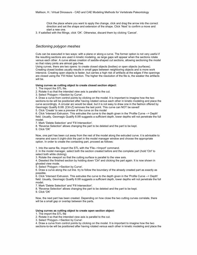
Mallison, H.: Virtual Dinosaurs - CAD and CAE Modeling Methods for Vertebrate Paleontology
Click the place where you want to apply the change, click and drag the arrow into the correct direction and set the shape and extension of the shape. Click ‘Next’ to confirm a move and start a new one.
3. If satisfied with the fillings, click ‘OK’. Otherwise, discard them by clicking ‘Cancel’.
Sectioning polygon meshes Cuts can be executed in two ways: with a plane or along a curve. The former option is not very useful if the resulting sections are used in kinetic modeling, as large gaps will appear when the sections rotate versus each other. A curve allows creation of saddle-shaped cut sections, allowing sectioning the model so that rotary joints are almost gap-free. Using curves, there are two opens: to create closed objects (bodies) or open objects (surfaces). Creating closed bodies usually results in small gaps between neighboring objects and is more work intensive. Creating open objects is faster, but carries a high risk of artifacts at the edges if the openings are closed using the ‘Fill Holes’ function. The higher the resolution of the file is, the weaker the artifacts will be. Using curves as cutting object to create closed section object: 1. The import the STL file. 2. Rotate it so that the intended view axis is parallel to the cut. 3. Select 'Polygon-->Section by Curve'. 4. Draw a curve from control points by clicking on the model. It is important to imagine how the two sections-to-be will be positioned after having rotated versus each other in kinetic modeling and place the curve accordingly. A circular arc would be ideal, but it is not easy to draw one in the fashion offered by Geomagic Qualify 8.0®. [Ctrl-Z] removes the last point. This curve can NOT be saved! 5. Click 'Create' to see a preview of the curve on the model 6. Click 'Intersect Extrusion. This extrudes the curve to the depth given in the 'Profile Curve --> Depth' field. Usually, Geomagic Qualify 8.0® suggests a sufficient depth, lower depths will not penetrate the full model. 7. Mark 'Delete Selection‘ and 'Fill Intersection'. 8. 'Reverse Selection' allows changing the part to be deleted and the part to be kept. 9. Click 'OK' Now, one part has been cut away from the rest of the model along the extruded curve. it is advisable to rename and save it (right-click the part in the model manager window and choose the appropriate option. In order to create the contacting part, proceed as follows: 1. Into the same file, import the STL with the 'File-->Import' command. 2. In the model manager, select both the section created before and the complete part (hold 'Ctrl' to select both while clicking). 3. Rotate the viewport so that the cutting surface is parallel to the view axis. 4. Deselect the finished section by holding down 'Ctrl' and clicking the part again. It is now shown in ghosted view mode. 5. Select 'Polygon-->Section by Curve'. 6. Draw a curve along the cut line. try to follow the boundary of the already created part as exactly as possible. 6. Click 'Intersect Extrusion. This extrudes the curve to the depth given in the 'Profile Curve --> Depth' field. Usually, Geomagic Qualify 8.0® suggests a sufficient depth, lower depths will not penetrate the full model. 7. Mark 'Delete Selection' and 'Fill Intersection'. 8. 'Reverse Selection' allows changing the part to be deleted and the part to be kept. 9. Click 'OK' Now, the next part has been created. Depending on how close the two cutting curves correlate, there will be a small gap or overlap between the parts. Using curves as cutting object to create open section object: 1. The import the STL file 2. Rotate it so that the intended view axis is parallel to the cut. 3. Select 'Polygon-->Section by Curve'. 4. Draw a curve from control points by clicking on the model. It is important to imagine how the two sections-to-be will be positioned after having rotated versus each other in kinetic modeling and place the
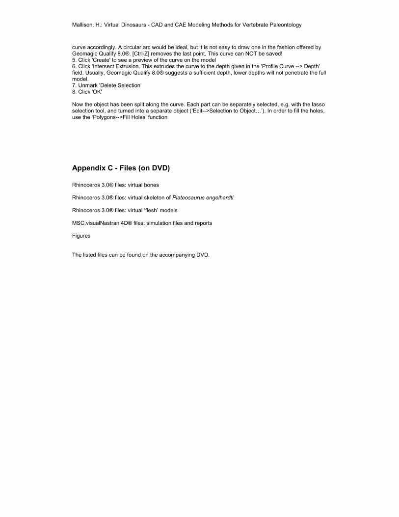
Mallison, H.: Virtual Dinosaurs - CAD and CAE Modeling Methods for Vertebrate Paleontology
curve accordingly. A circular arc would be ideal, but it is not easy to draw one in the fashion offered by Geomagic Qualify 8.0®. [Ctrl-Z] removes the last point. This curve can NOT be saved! 5. Click 'Create' to see a preview of the curve on the model 6. Click 'Intersect Extrusion. This extrudes the curve to the depth given in the 'Profile Curve --> Depth' field. Usually, Geomagic Qualify 8.0® suggests a sufficient depth, lower depths will not penetrate the full model. 7. Unmark 'Delete Selection‘ 8. Click 'OK' Now the object has been split along the curve. Each part can be separately selected, e.g. with the lasso selection tool, and turned into a separate object (‘Edit-->Selection to Object…’). In order to fill the holes, use the ‘Polygons-->Fill Holes’ function
Appendix C - Files (on DVD)
Rhinoceros 3.0® files: virtual bones Rhinoceros 3.0® files: virtual skeleton of Plateosaurus engelhardti Rhinoceros 3.0® files: virtual ‘flesh’ models MSC.visualNastran 4D® files: simulation files and reports Figures The listed files can be found on the accompanying DVD.