workshop on empirical likelihood methods in survival analysis

Workshop on Empirical LikelihoodMethods in Survival Analysis

Ian McKeague

Department of Statistics

Florida State University

Tallahassee, FL 32306-4330, USA

<http://stat.fsu.edu/∼mckeague>

2

Outline

• Background on empirical likelihood (EL)

• Background on survival analysis

• EL methods in one-sample problems with censoring

• Two-sample problems

Louvain-la-Neuve Workshop May, 2002

3

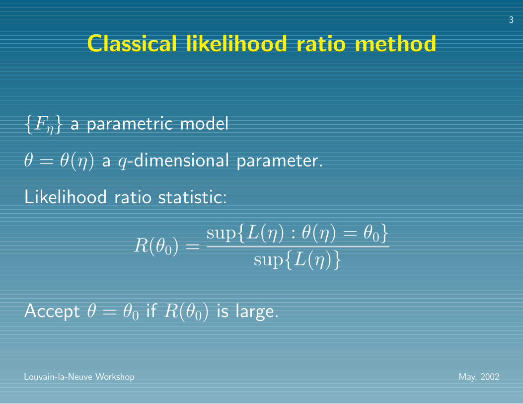
Classical likelihood ratio method

{Fη} a parametric model

θ = θ(η) a q-dimensional parameter.

Likelihood ratio statistic:

R(θ0) =sup{L(η) : θ(η) = θ0}

sup{L(η)}

Accept θ = θ0 if R(θ0) is large.


4

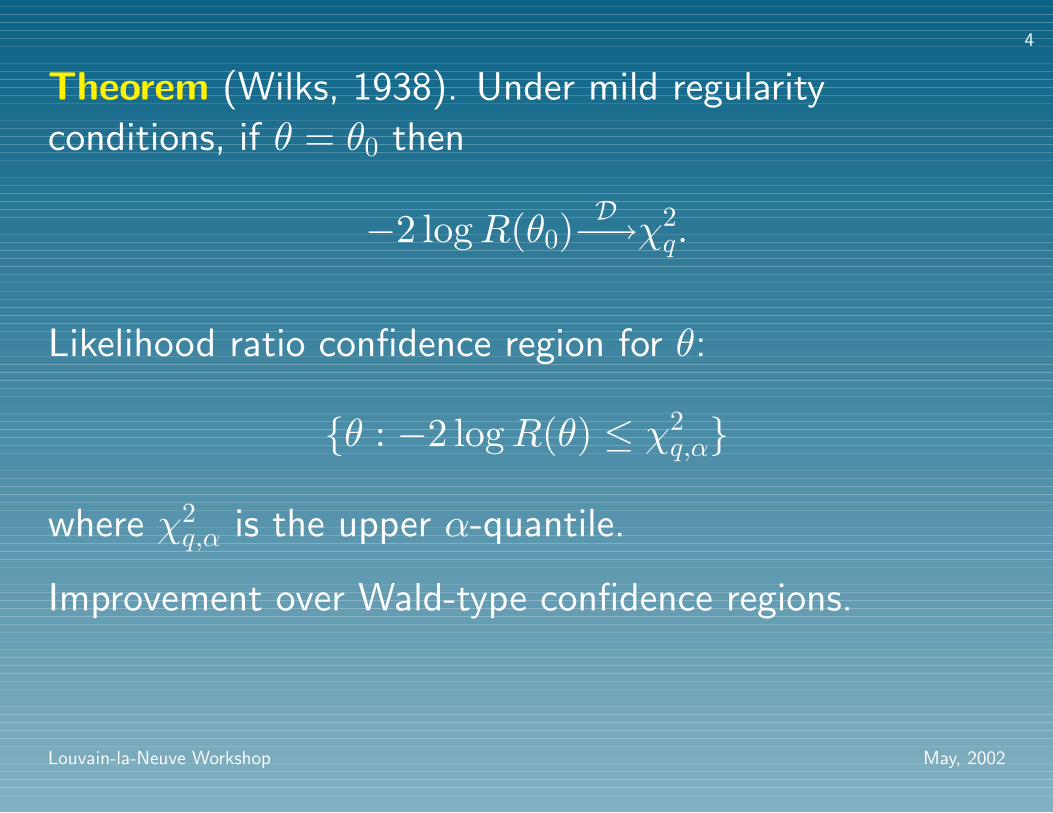
Theorem (Wilks, 1938). Under mild regularity

conditions, if θ = θ0 then

−2 logR(θ0)D−→χ2

q.

Likelihood ratio confidence region for θ:

{θ : −2 logR(θ) ≤ χ2q,α}

where χ2q,α is the upper α-quantile.

Improvement over Wald-type confidence regions.


5

Background on Empirical likelihood

• Thomas and Grunkemeier (1975) for survival function

estimation. Owen (1988, 1990, . . . , 2001).

• First developed for finite-dimensional features θ = θ(F )of a cdf (e.g., mean, median, cdf at a single point).


6

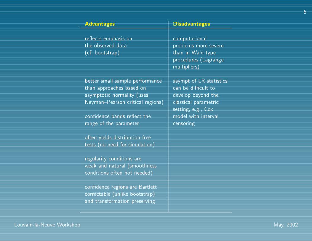
Advantages Disadvantages

reflects emphasis on computationalthe observed data problems more severe(cf. bootstrap) than in Wald type

procedures (Lagrangemultipliers)

better small sample performance asympt of LR statisticsthan approaches based on can be difficult toasymptotic normality (uses develop beyond theNeyman–Pearson critical regions) classical parametric

setting, e.g., Coxconfidence bands reflect the model with intervalrange of the parameter censoring

often yields distribution-freetests (no need for simulation)

regularity conditions areweak and natural (smoothnessconditions often not needed)

confidence regions are Bartlettcorrectable (unlike bootstrap)and transformation preserving


7

Empirical cdf

Fn(x) =1n

n∑i=1

1{Xi ≤ x}

Nonparametric likelihood

L(F ) =n∏i=1

(F (Xi)− F (Xi−)).

Fn is the NPMLE:

Fn = arg maxF

L(F )


8

EL ratio

R(F ) =L(F )L(Fn)

=n∏i=1

npi

where (part of) the mass on Xi is pi ≥ 0,∑n

i=1 pi ≤ 1.

To maximize R(F ), only need consider F supported on

the data, i.e.,n∑i=1

pi = 1.


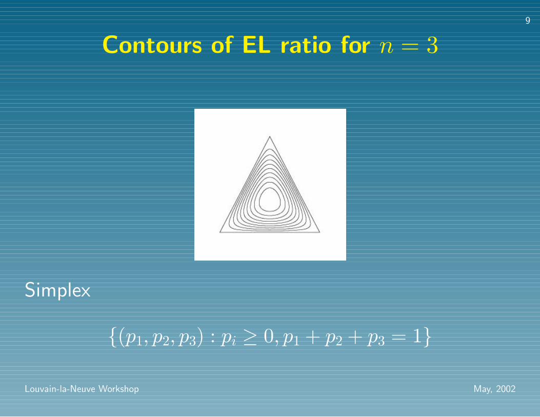
9

Contours of EL ratio for n = 3

Simplex

{(p1, p2, p3) : pi ≥ 0, p1 + p2 + p3 = 1}


10

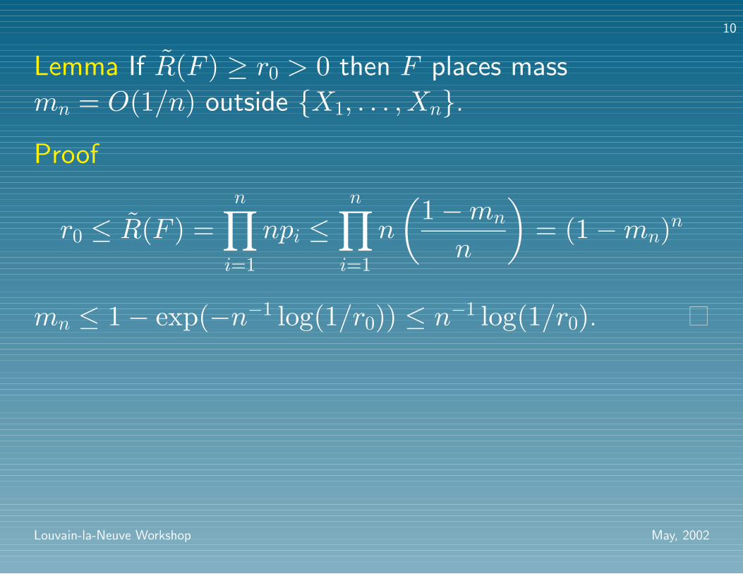
Lemma If R(F ) ≥ r0 > 0 then F places mass

mn = O(1/n) outside {X1, . . . , Xn}.

Proof

r0 ≤ R(F ) =n∏i=1

npi ≤n∏i=1

n

(1−mn

n

)= (1−mn)n

mn ≤ 1− exp(−n−1 log(1/r0)) ≤ n−1 log(1/r0).


11

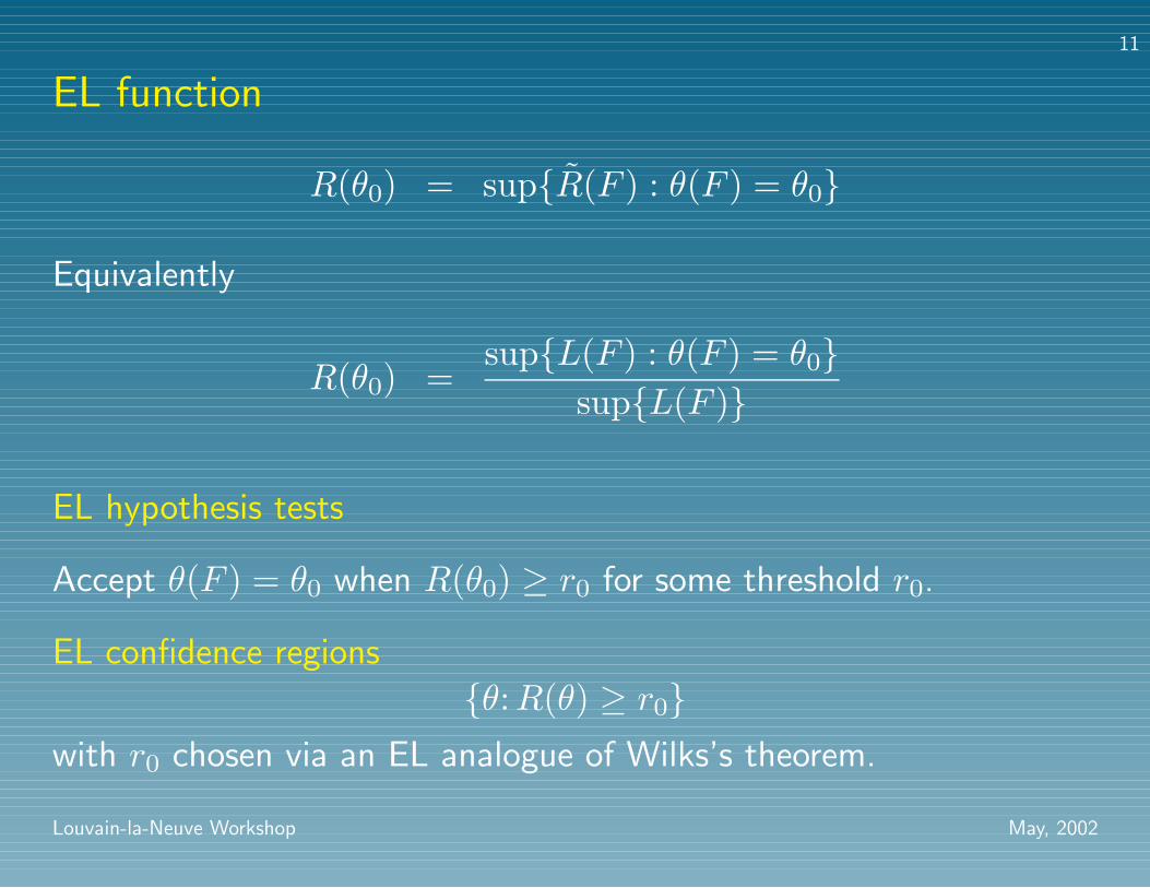
EL function

R(θ0) = sup{R(F ) : θ(F ) = θ0}

Equivalently

R(θ0) =sup{L(F ) : θ(F ) = θ0}

sup{L(F )}

EL hypothesis tests

Accept θ(F ) = θ0 when R(θ0) ≥ r0 for some threshold r0.

EL confidence regions

{θ:R(θ) ≥ r0}with r0 chosen via an EL analogue of Wilks’s theorem.


12

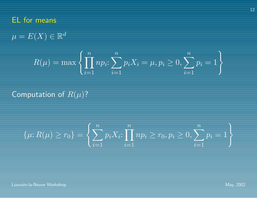
EL for means

µ = E(X) ∈ Rd

R(µ) = max

{n∏i=1

npi:n∑i=1

piXi = µ, pi ≥ 0,n∑i=1

pi = 1

}

Computation of R(µ)?

{µ:R(µ) ≥ r0} =

{n∑i=1

piXi:n∏i=1

npi ≥ r0, pi ≥ 0,n∑i=1

pi = 1

}


13

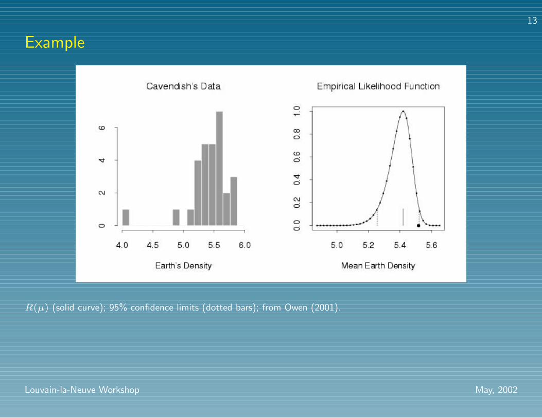
Example

R(µ) (solid curve); 95% confidence limits (dotted bars); from Owen (2001).


14

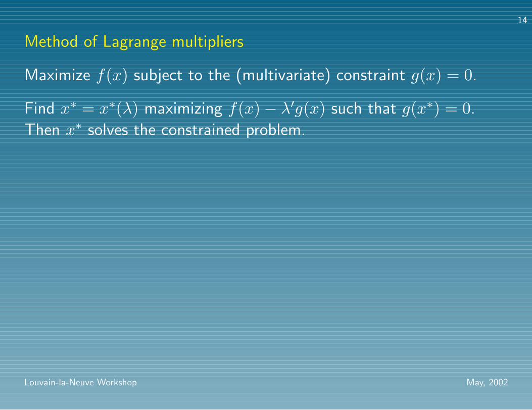
Method of Lagrange multipliers

Maximize f(x) subject to the (multivariate) constraint g(x) = 0.

Find x∗ = x∗(λ) maximizing f(x)− λ′g(x) such that g(x∗) = 0.

Then x∗ solves the constrained problem.


15

Geometric intuition available when g is univariate

At the maximum, ∇f and ∇g must be parallel: ∇f = λ∇g for some

constant λ (Lagrange multiplier).


16

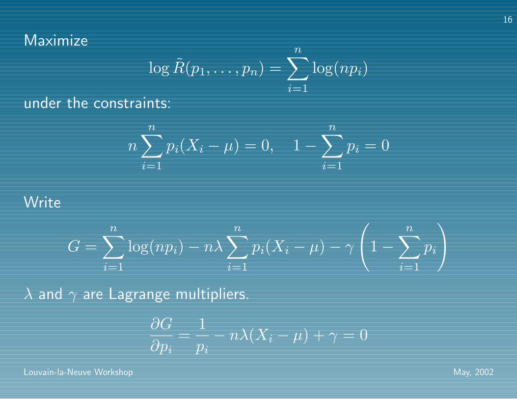
Maximize

log R(p1, . . . , pn) =n∑i=1

log(npi)

under the constraints:

nn∑i=1

pi(Xi − µ) = 0, 1−n∑i=1

pi = 0

Write

G =n∑i=1

log(npi)− nλn∑i=1

pi(Xi − µ)− γ

(1−

n∑i=1

pi

)λ and γ are Lagrange multipliers.

∂G

∂pi=

1pi− nλ(Xi − µ) + γ = 0


17

so

0 =n∑i=1

pi∂G

∂pi= n+ γ

giving γ = −n. Thus

pi =1n

11 + λ(Xi − µ)

Plugging this back into the constraint:

g(λ) =1n

n∑i=1

Xi − µ1 + λ(Xi − µ)

= 0

This equation has a unique solution for λ = λ(µ).


18

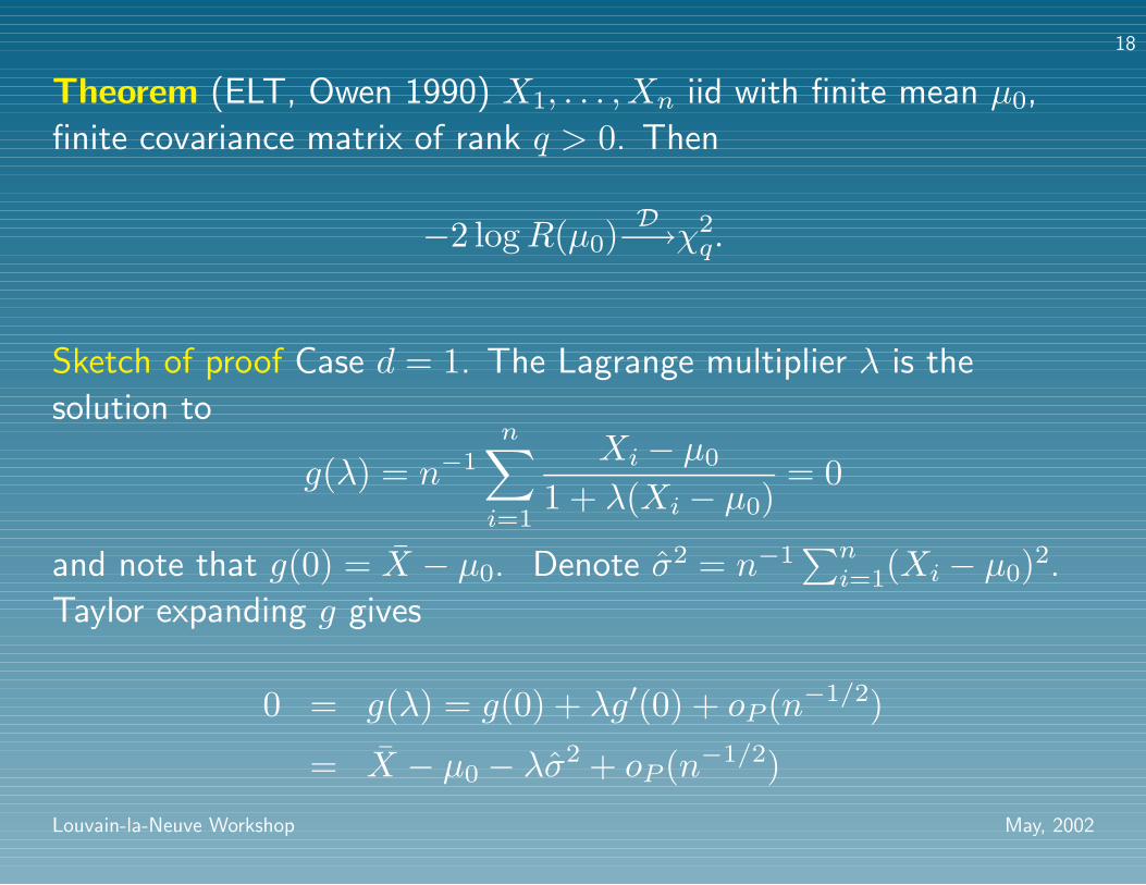
Theorem (ELT, Owen 1990) X1, . . . , Xn iid with finite mean µ0,

finite covariance matrix of rank q > 0. Then

−2 logR(µ0) D−→χ2q.

Sketch of proof Case d = 1. The Lagrange multiplier λ is the

solution to

g(λ) = n−1n∑i=1

Xi − µ0

1 + λ(Xi − µ0)= 0

and note that g(0) = X − µ0. Denote σ2 = n−1∑ni=1(Xi − µ0)2.

Taylor expanding g gives

0 = g(λ) = g(0) + λg′(0) + oP (n−1/2)

= X − µ0 − λσ2 + oP (n−1/2)


19

Thus λ = (X − µ0)/σ2 + oP (n−1/2) = OP (n−1/2). Recall

pi =1n

11 + λ(Xi − µ0)

so, using the Taylor expansion log(1 + x) = x− x2/2 +O(x3),

−2 logR(µ0) = −2n∑i=1

log(npi) = 2n∑i=1

log(1 + λ(Xi − µ0))

= 2nλ(X − µ0)− nλ2σ2 + oP (1)

= 2n(X − µ0)2/σ2 − n(X − µ0)2/σ2 + oP (1)

= n(X − µ0)2/σ2 + oP (1)D−→ χ2

1


20

This suggests the χ2-calibration with threshold

r0 = exp(−χ2q,α/2)

for a 100(1− α)% confidence region; actual coverage

1− α+O(n−1).

Fisher calibrationd(n− 1)n− d

Fd,n−d,α

Bartlett correction (1 +

a

n

)χ2q,α

a involves higher-order moments of X, and needs to be estimated.

Coverage improves to 1− α+O(n−2).


21

Bootstrap calibration

X∗1 , . . . , X∗n iid from Fn. Simulation used to find the upper

α-quantile of −2 logR∗(X), where

R∗(X) = max

{n∏i=1

npi:n∑i=1

piX∗i = X, pi ≥ 0,

n∑i=1

pi = 1

}


22

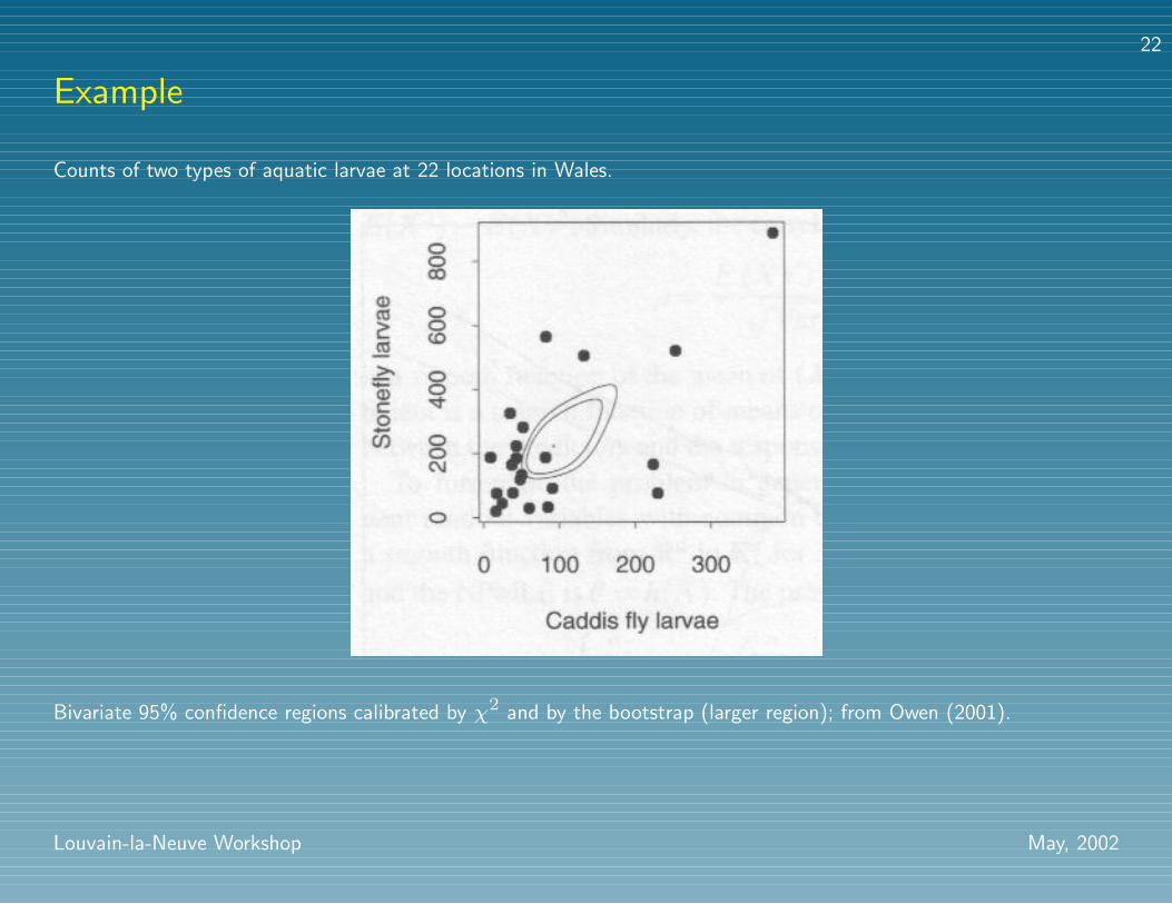
Example

Counts of two types of aquatic larvae at 22 locations in Wales.

Bivariate 95% confidence regions calibrated by χ2 and by the bootstrap (larger region); from Owen (2001).


23

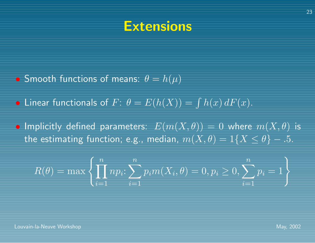
Extensions

• Smooth functions of means: θ = h(µ)

• Linear functionals of F : θ = E(h(X)) =∫h(x) dF (x).

• Implicitly defined parameters: E(m(X, θ)) = 0 where m(X, θ) is

the estimating function; e.g., median, m(X, θ) = 1{X ≤ θ} − .5.

R(θ) = max

{n∏i=1

npi:n∑i=1

pim(Xi, θ) = 0, pi ≥ 0,n∑i=1

pi = 1

}


24

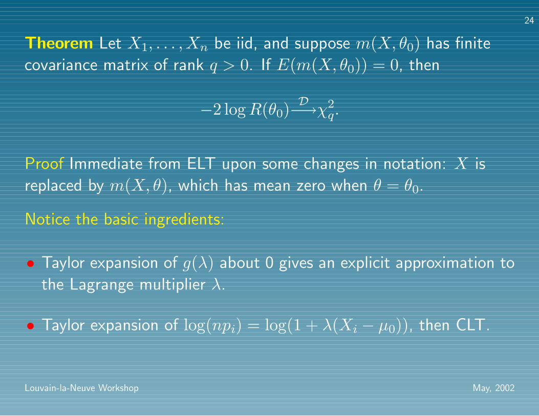
Theorem Let X1, . . . , Xn be iid, and suppose m(X, θ0) has finite

covariance matrix of rank q > 0. If E(m(X, θ0)) = 0, then

−2 logR(θ0) D−→χ2q.

Proof Immediate from ELT upon some changes in notation: X is

replaced by m(X, θ), which has mean zero when θ = θ0.

Notice the basic ingredients:

• Taylor expansion of g(λ) about 0 gives an explicit approximation to

the Lagrange multiplier λ.

• Taylor expansion of log(npi) = log(1 + λ(Xi − µ0)), then CLT.


25

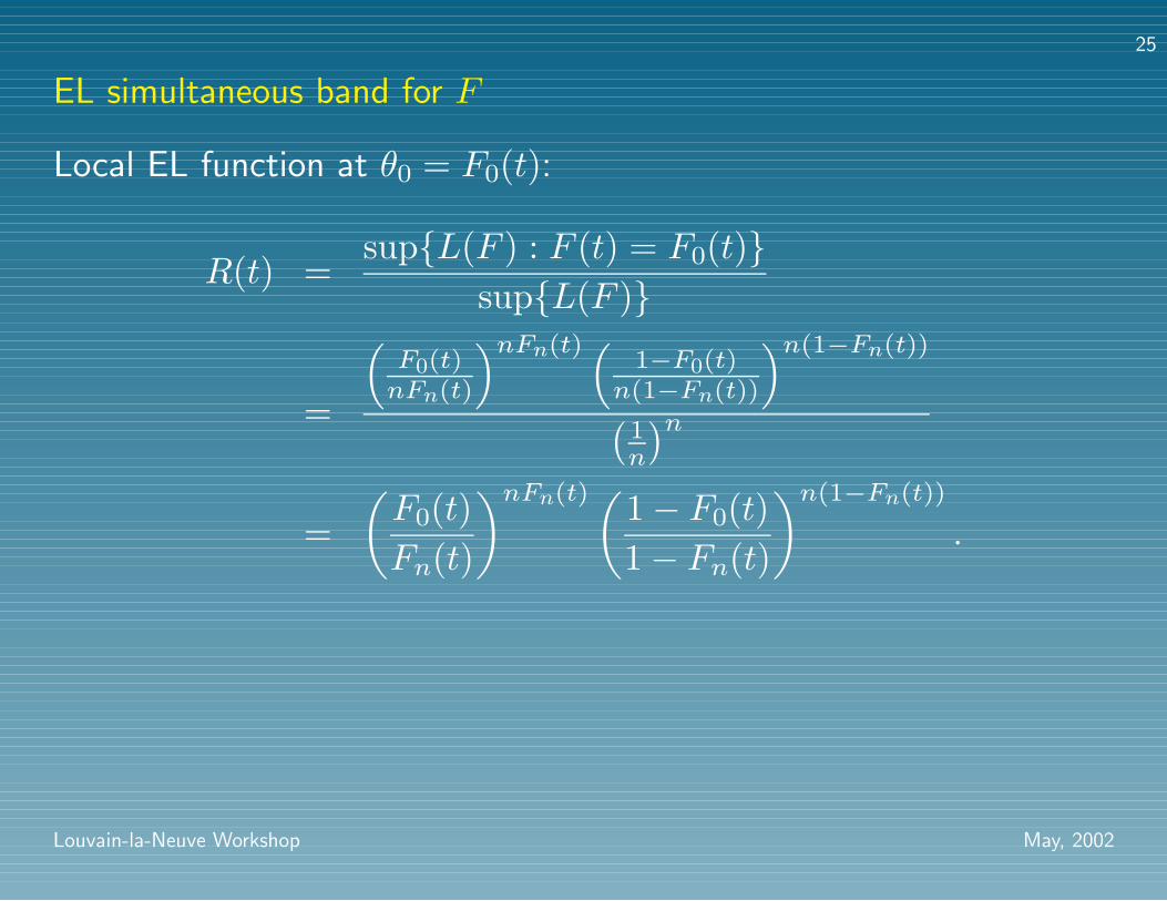
EL simultaneous band for F

Local EL function at θ0 = F0(t):

R(t) =sup{L(F ) : F (t) = F0(t)}

sup{L(F )}

=

(F0(t)nFn(t)

)nFn(t) (1−F0(t)

n(1−Fn(t))

)n(1−Fn(t))

(1n

)n=(F0(t)Fn(t)

)nFn(t)(1− F0(t)1− Fn(t)

)n(1−Fn(t))

.


26

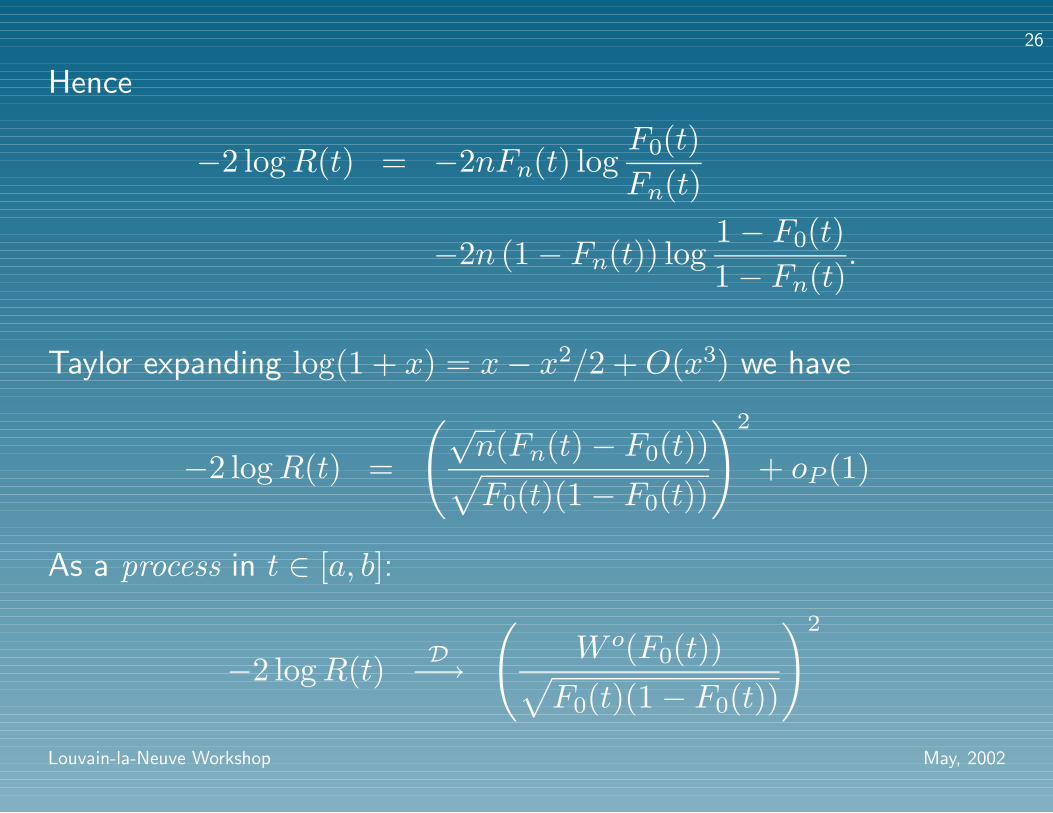
Hence

−2 logR(t) = −2nFn(t) logF0(t)Fn(t)

−2n (1− Fn(t)) log1− F0(t)1− Fn(t)

.

Taylor expanding log(1 + x) = x− x2/2 +O(x3) we have

−2 logR(t) =

(√n(Fn(t)− F0(t))√F0(t)(1− F0(t))

)2

+ oP (1)

As a process in t ∈ [a, b]:

−2 logR(t) D−→

(W o(F0(t))√

F0(t)(1− F0(t))

)2


27

D=(W (σ2(t))σ(t)

)2

,

W o standard tied-down Wiener process (Brownian bridge)

W standard Wiener process

σ2(t) =F0(t)

1− F0(t).


28

Simultaneous confidence band for F over an interval [a, b]:

{(t, F0(t)) : −2 logR(t) ≤ Cα, t ∈ [a, b]}

Cα the upper α-quantile of

supt∈[σ2(a),σ2(b)]

W 2(t)t

.

Equal precision LR band. Narrower in tail than Hollander, McKeague, Yang (1997) band.


29

EL test for F = F0

Tn = −2∫ ∞−∞

logR(t) dFn(t)

D−→∫ 1

0

(W o(t)√t(1− t)

)2

dt.


30

EL test for symmetry Einmahl and McKeague (2001): EL tests for symmetry, exponentiality,

independence and changes in distribution.

H0 : F (−x) = 1− F (x−), for all x > 0.

Local EL function:

R(x) =sup{L(F ) : F (−x) = 1− F (x−)}

sup{L(F )}, x > 0.

Treat F as a function of 0 ≤ p ≤ 1, where F puts mass

• p/2 on (−∞,−x], and on [x,∞)

• 1− p on (−x, x)


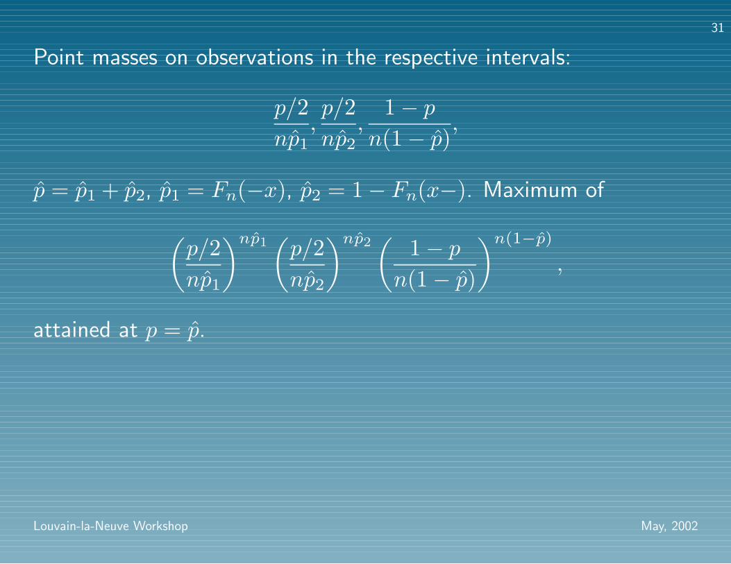
31

Point masses on observations in the respective intervals:

p/2np1

,p/2np2

,1− p

n(1− p),

p = p1 + p2, p1 = Fn(−x), p2 = 1− Fn(x−). Maximum of(p/2np1

)np1(p/2np2

)np2(

1− pn(1− p)

)n(1−p)

,

attained at p = p.


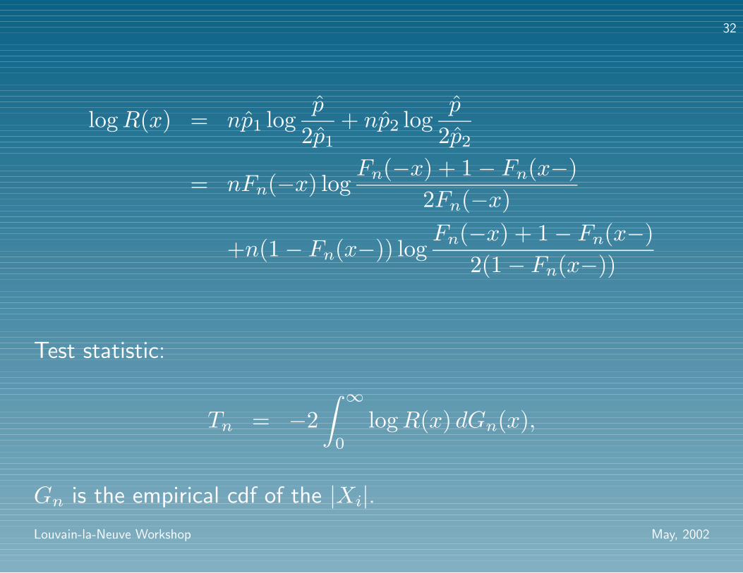
32

logR(x) = np1 logp

2p1+ np2 log

p

2p2

= nFn(−x) logFn(−x) + 1− Fn(x−)

2Fn(−x)

+n(1− Fn(x−)) logFn(−x) + 1− Fn(x−)

2(1− Fn(x−))

Test statistic:

Tn = −2∫ ∞

0

logR(x) dGn(x),

Gn is the empirical cdf of the |Xi|.Louvain-la-Neuve Workshop May, 2002

33

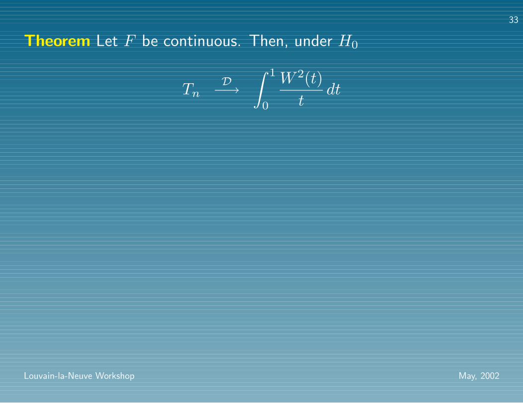
Theorem Let F be continuous. Then, under H0

TnD−→

∫ 1

0

W 2(t)t

dt


34

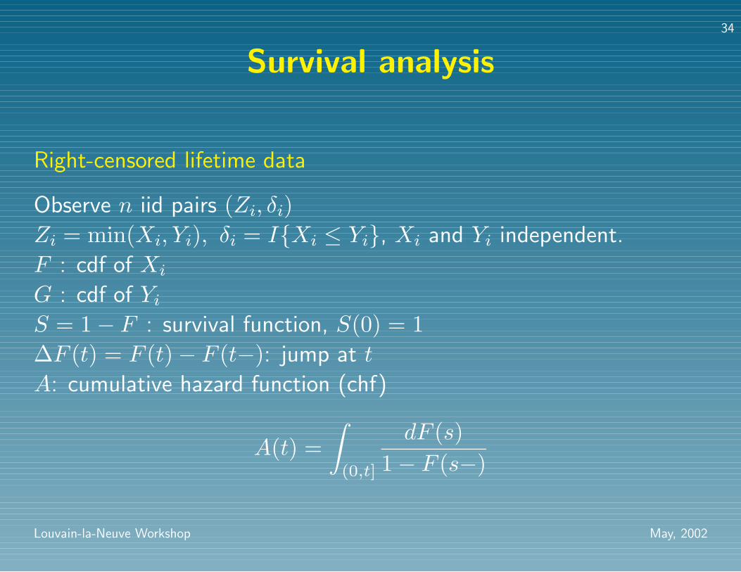
Survival analysis

Right-censored lifetime data

Observe n iid pairs (Zi, δi)Zi = min(Xi, Yi), δi = I{Xi ≤ Yi}, Xi and Yi independent.

F : cdf of Xi

G : cdf of YiS = 1− F : survival function, S(0) = 1∆F (t) = F (t)− F (t−): jump at t

A: cumulative hazard function (chf)

A(t) =∫

(0,t]

dF (s)1− F (s−)


35

Review of some basics

There is a 1-1 correspondence between survival functions and

cumulative hazards. If F is continuous: A = − log(S),

S = exp(−A).

Lemma If F is a discrete cdf, the corresponding cumulative hazard

function is

A(t) =∑s≤t

∆F (s)1− F (s−)

.

Conversely, if A is a discrete chf, the corresponding survival function

is

S(t) =∏s≤t

(1−∆A(t))


36

Proof Given a discrete chf A, write S(t) =∏s≤t(1−∆A(t)). Then

S has chf A, because S(t−) = S(t)/(1−∆A(t)) and

∆A(t) = 1− S(t)S(t−)

=∆F (s)

1− F (s−).

Conversely, given a discrete survival function S, then

S(t) =∏u≤t

S(u)S(u−)

=∏u≤t

(1 +

∆S(u)S(u−)

)=

∏u≤t

(1−∆A(u))

where A is the chf.


37

Hazard functions

If F has density f , define the hazard function

α(t) = f(t)/S(t) ≈ P (X ∈ [t, t+ dt)|X ≥ t)/dt

Thus

P (X ∈ [t, t+ dt)|X ≥ t) ≈ α(t) dt

Cox proportional hazards model

α(t|z) = α0(t) exp(β′z)

adjusts for a (multi-dimensional) covariate z.


38

Counting process approach

N(t) = 1{Z ≤ t, δ = 1}

At risk indicator: Y (t) = 1{Z ≥ t}

Basic martingale: M(t) = N(t)−∫ t

0Y (s)α(s) ds

dN(t) ∼ Bernoulli(Y (t)α(t) dt) given the past, so

E(dM(t)|past) = E(dN(t)− Y (t)α(t) dt|past) = 0


39

Nonparametric likelihood

L(S) = L(F ) =n∏i=1

(F (Zi)− F (Zi−))δi(1− F (Zi))1−δi.

To maximize L(F ), we only need consider F supported on the

uncensored lifetimes.


40

Notation

Ordered uncensored lifetimes: 0 < T1 ≤ . . . ≤ Tk, T0 = 0hj = ∆A(Tj) = 1− S(Tj)/S(Tj−1) jump in chf at Tjrj =

∑ni=1 1{Zi ≥ Tj} size of the risk set at Tj−, with rk+1 = 0.

dj ≥ 1 denotes the number of uncensored failures at Tj.

Lemma If F is supported on the uncensored lifetimes, then

L(S) =k∏j=1

hdjj (1− hj)rj−dj


41

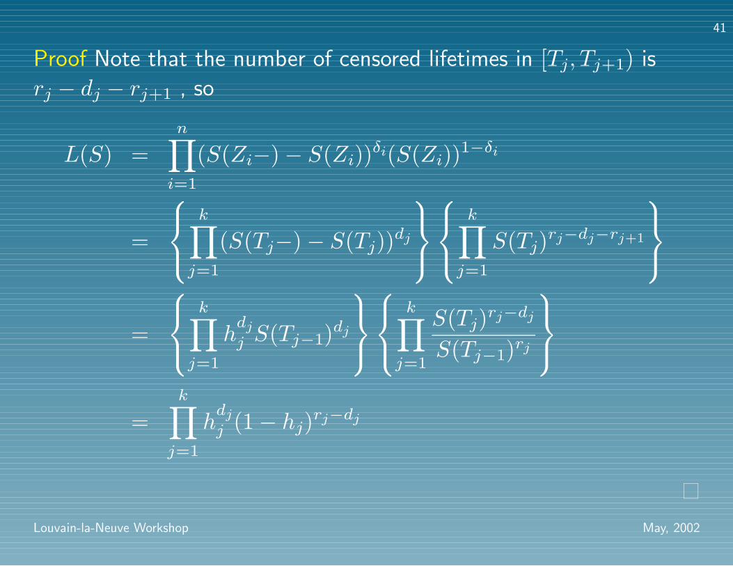
Proof Note that the number of censored lifetimes in [Tj, Tj+1) is

rj − dj − rj+1 , so

L(S) =n∏i=1

(S(Zi−)− S(Zi))δi(S(Zi))1−δi

=

k∏j=1

(S(Tj−)− S(Tj))dj

k∏j=1

S(Tj)rj−dj−rj+1

=

k∏j=1

hdjj S(Tj−1)dj

k∏j=1

S(Tj)rj−dj

S(Tj−1)rj

=

k∏j=1

hdjj (1− hj)rj−dj


42

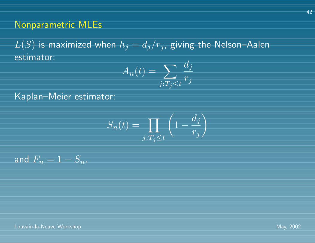
Nonparametric MLEs

L(S) is maximized when hj = dj/rj, giving the Nelson–Aalen

estimator:

An(t) =∑j:Tj≤t

djrj

Kaplan–Meier estimator:

Sn(t) =∏j:Tj≤t

(1− dj

rj

)

and Fn = 1− Sn.


43

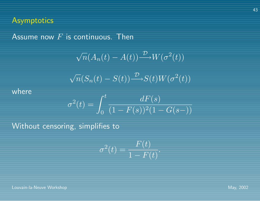
Asymptotics

Assume now F is continuous. Then

√n(An(t)−A(t)) D−→W (σ2(t))

√n(Sn(t)− S(t)) D−→S(t)W (σ2(t))

where

σ2(t) =∫ t

0

dF (s)(1− F (s))2(1−G(s−))

Without censoring, simplifies to

σ2(t) =F (t)

1− F (t).


44

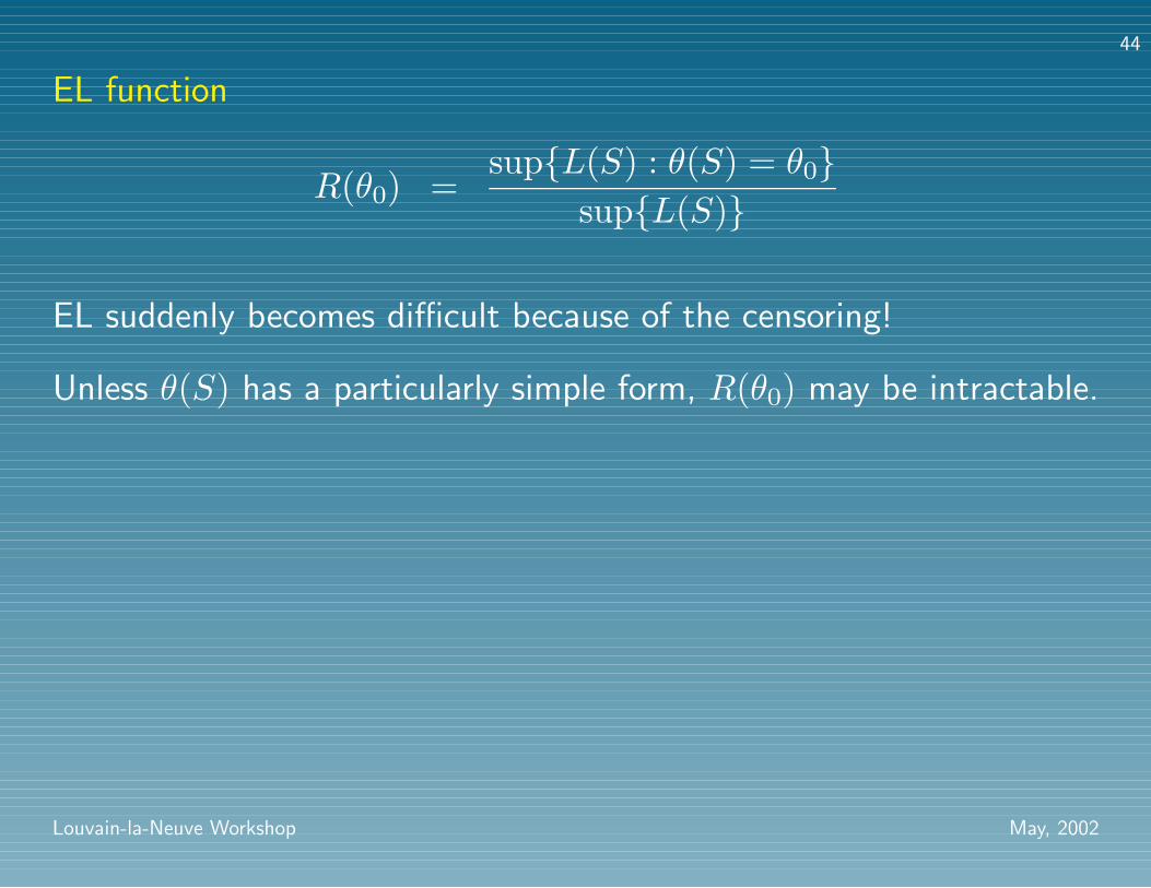
EL function

R(θ0) =sup{L(S) : θ(S) = θ0}

sup{L(S)}

EL suddenly becomes difficult because of the censoring!

Unless θ(S) has a particularly simple form, R(θ0) may be intractable.


45

Known tractable forms of θ(S) or θ(A):

• S(t0)

• A(t0)

• quantiles

• linear functionals θ(F ) =∫h(t) dF (t)

• linear functionals θ(A) =∫h(t) dA(t)

Thomas and Grunkemeier (1975), Li (1995), Murphy (1995), Pan and Zhou (2002)


46

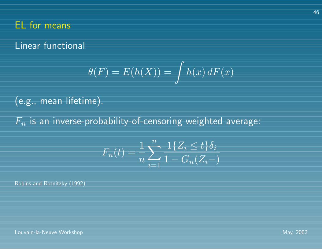
EL for means

Linear functional

θ(F ) = E(h(X)) =∫h(x) dF (x)

(e.g., mean lifetime).

Fn is an inverse-probability-of-censoring weighted average:

Fn(t) =1n

n∑i=1

1{Zi ≤ t}δi1−Gn(Zi−)

Robins and Rotnitzky (1992)


47

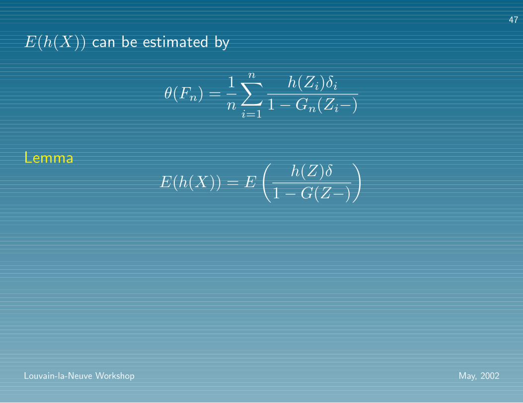
E(h(X)) can be estimated by

θ(Fn) =1n

n∑i=1

h(Zi)δi1−Gn(Zi−)

Lemma

E(h(X)) = E

(h(Z)δ

1−G(Z−)

)


48

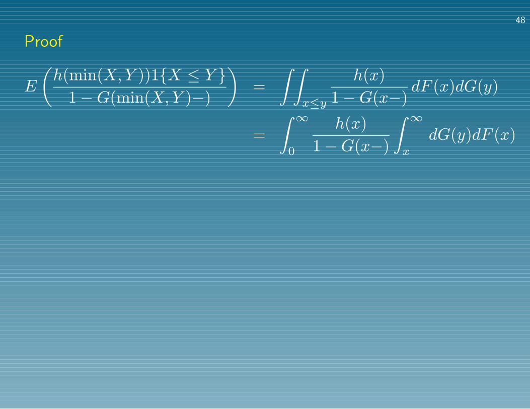
Proof

E

(h(min(X,Y ))1{X ≤ Y }

1−G(min(X,Y )−)

)=∫ ∫

x≤y

h(x)1−G(x−)

dF (x)dG(y)

=∫ ∞

0

h(x)1−G(x−)

∫ ∞x

dG(y)dF (x)

48

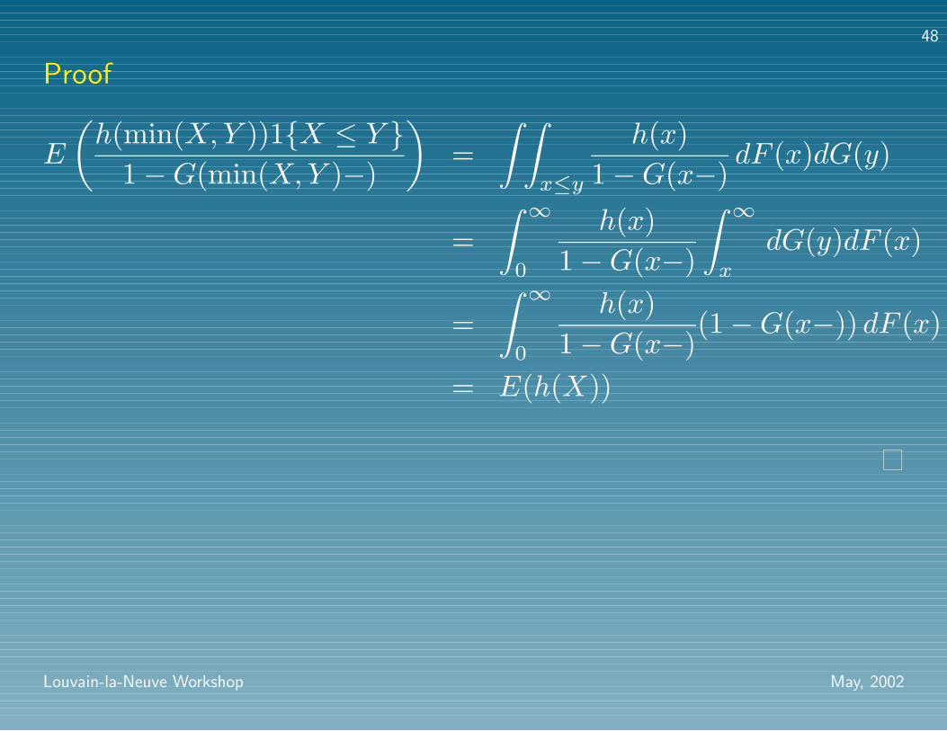
Proof

E

(h(min(X,Y ))1{X ≤ Y }

1−G(min(X,Y )−)

)=∫ ∫

x≤y

h(x)1−G(x−)

dF (x)dG(y)

=∫ ∞

0

h(x)1−G(x−)

∫ ∞x

dG(y)dF (x)

=∫ ∞

0

h(x)1−G(x−)

(1−G(x−)) dF (x)

= E(h(X))


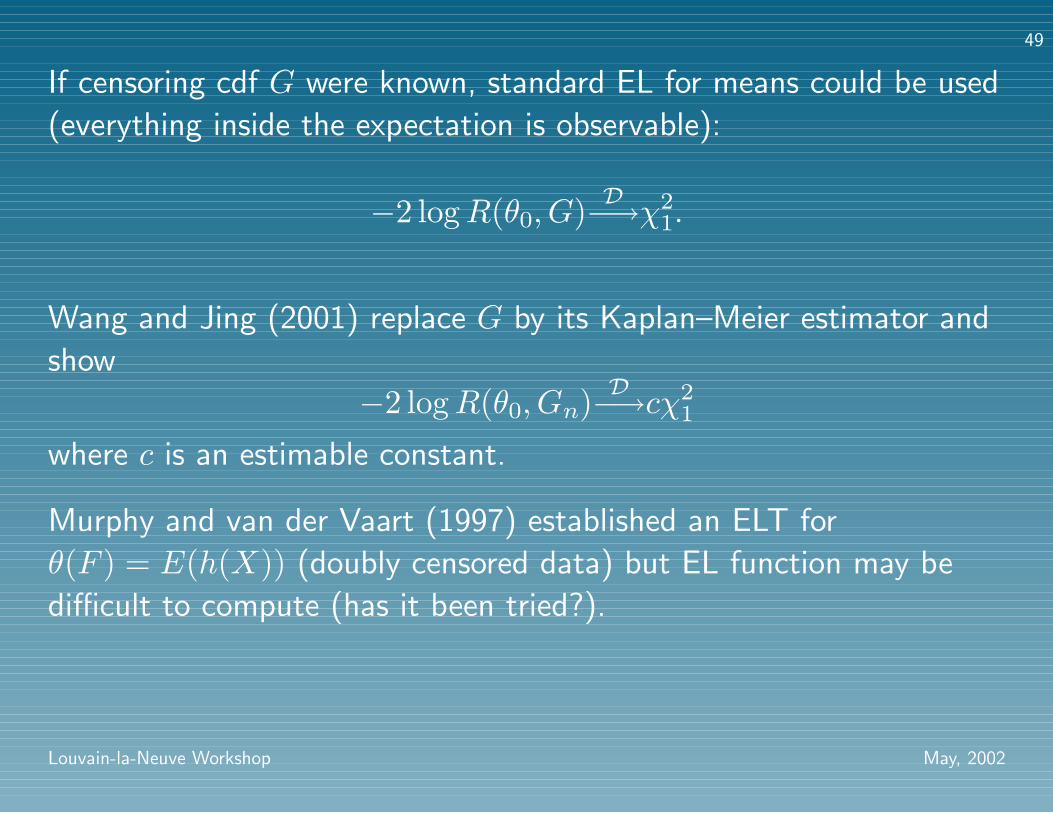
49

If censoring cdf G were known, standard EL for means could be used

(everything inside the expectation is observable):

−2 logR(θ0, G) D−→χ21.

Wang and Jing (2001) replace G by its Kaplan–Meier estimator and

show

−2 logR(θ0, Gn) D−→cχ21

where c is an estimable constant.

Murphy and van der Vaart (1997) established an ELT for

θ(F ) = E(h(X)) (doubly censored data) but EL function may be

difficult to compute (has it been tried?).


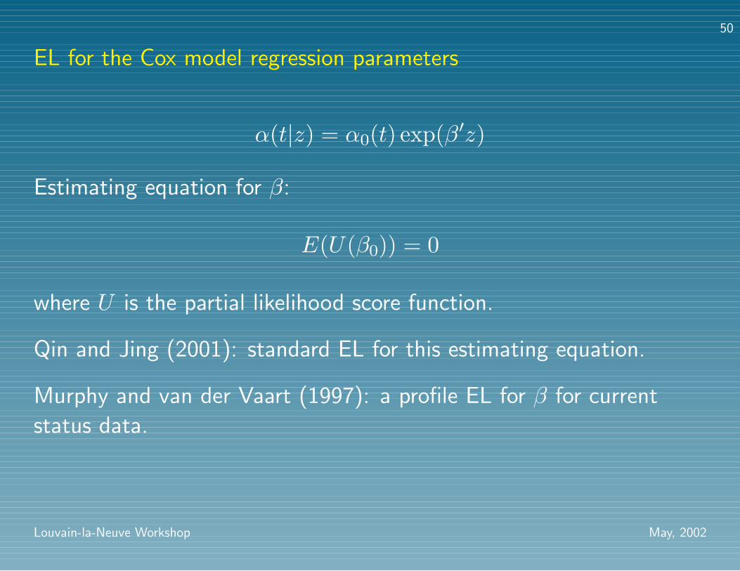
50

EL for the Cox model regression parameters

α(t|z) = α0(t) exp(β′z)

Estimating equation for β:

E(U(β0)) = 0

where U is the partial likelihood score function.

Qin and Jing (2001): standard EL for this estimating equation.

Murphy and van der Vaart (1997): a profile EL for β for current

status data.


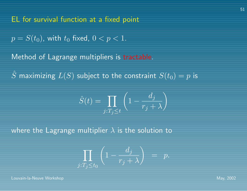
51

EL for survival function at a fixed point

p = S(t0), with t0 fixed, 0 < p < 1.

Method of Lagrange multipliers is tractable.

S maximizing L(S) subject to the constraint S(t0) = p is

S(t) =∏j:Tj≤t

(1− dj

rj + λ

)

where the Lagrange multiplier λ is the solution to

∏j:Tj≤t0

(1− dj

rj + λ

)= p.


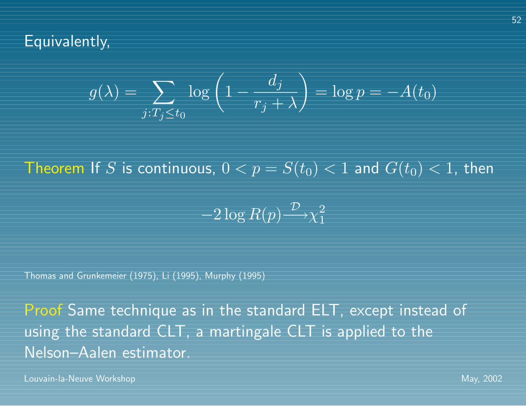
52

Equivalently,

g(λ) =∑

j:Tj≤t0

log(

1− djrj + λ

)= log p = −A(t0)

Theorem If S is continuous, 0 < p = S(t0) < 1 and G(t0) < 1, then

−2 logR(p) D−→χ21

Thomas and Grunkemeier (1975), Li (1995), Murphy (1995)

Proof Same technique as in the standard ELT, except instead of

using the standard CLT, a martingale CLT is applied to the

Nelson–Aalen estimator.


53

Taylor expansion of g leads to

λ = n(A(t0)−An(t0))/σ2 +OP (1)

where σ2 is an estimate of σ2(t0).

−2 logR(p) = −2(log(L(S)− log(L(Sn))

= −2∑

i:Tj≤t0

{(rj − dj) log

(1 +

λ

rj − dj

)

−rj log(

1 +λ

rj

)}= λ2σ2/n+ oP (1)

= n(An(t0)−A(t0))2/σ2 + oP (1)D−→ χ2

1


54

EL simultaneous band for S

As a process in t ∈ [a, b],

−2 logR(t) D−→(W (σ2(t))σ(t)

)2

,

Simultaneous confidence band for S over an interval [a, b]:

{(t, S(t)) : −2 logR(t) ≤ Cα, t ∈ [a, b]}

Cα the upper α-quantile of

supt∈[σ2(a),σ2(b)]

W 2(t)t

Equal precision LR band. Narrower in the tail than Hollander, McKeague, Yang (1997) band.

Li and Van Keilegom (2001): adjustment for a covariate effect (continuous one-dimensional covariate).


55

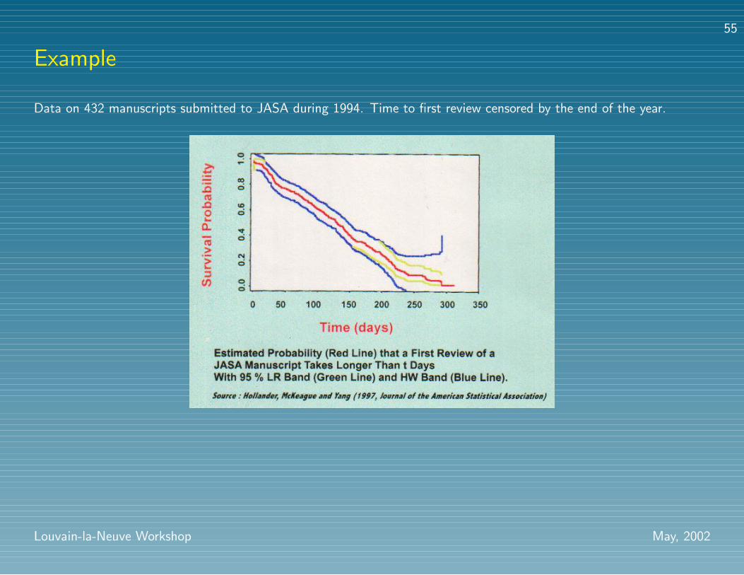
Example

Data on 432 manuscripts submitted to JASA during 1994. Time to first review censored by the end of the year.


56

Two-sample problem with censoring

Comparison of treatment and placebo groups.

Notation

Index sample by j

Assume nj/n→ pj > 0Total sample size n = n1 + n2

Nonparametric likelihood: L(S1, S2) = L1(S1)L2(S2).


57

• Standard method: logrank test for S1 = S2.

• Wald-type comparison of S1 and S2 using some smooth functio-

nal ϕ(S1, S2) and the functional delta method typically leads to

intractable limiting distributions. Simulation needed.

Gaussian multiplier simulation technique

Martingale increments dMi(t) replaced by GidNi(t), where

Gi ∼ N(0, 1). (Lin, Wei and Ying, 1993)

Parzen, Wei and Ying (1997) constructed a Wald-type confidence

band for S1(t)− S2(t) using this technique.


58

Q-Q plot

{(F−11 (p), F−1

2 (p)) : 0 < p < 1}

Einmahl and McKeague (1999) constructed an EL confidence band

for the Q-Q plot:

{(t1, t2):−2 logR(t1, t2) ≤ Cα, t1 ∈ [a, b]}

where Cα uses

σ2(t) = σ21(t)/p1 + σ2

2(t′)/p2

and t′ = F−12 (F1(t)). Simulation not needed.


59

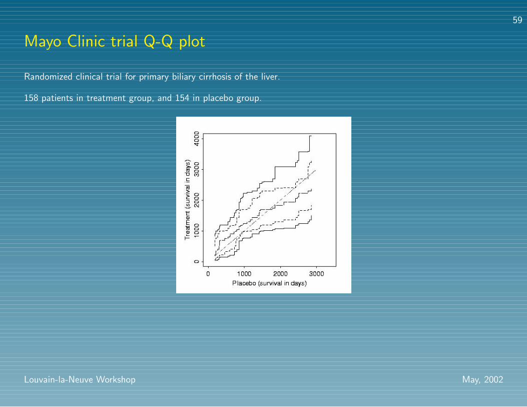
Mayo Clinic trial Q-Q plot

Randomized clinical trial for primary biliary cirrhosis of the liver.

158 patients in treatment group, and 154 in placebo group.


60

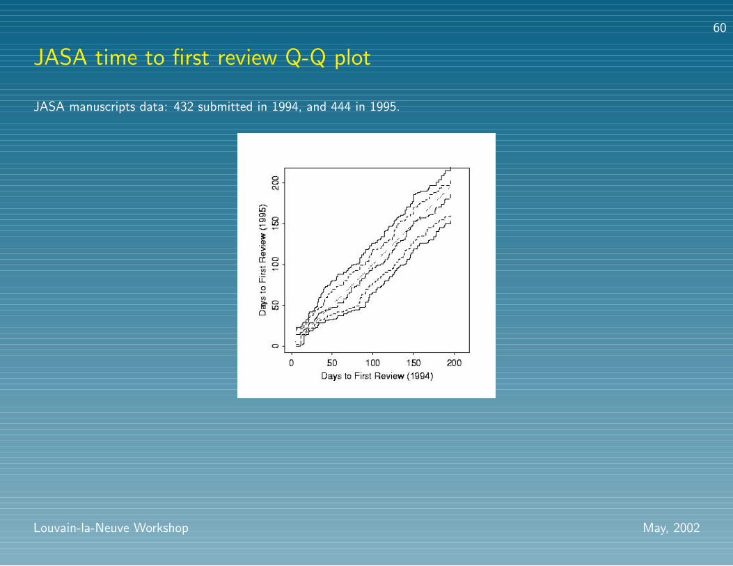
JASA time to first review Q-Q plot

JASA manuscripts data: 432 submitted in 1994, and 444 in 1995.


61

Relative survival

θ(t) = S1(t)/S2(t)

More relevant than a Q-Q plot to medical practice and easier to

interpret.

McKeague and Zhao (2002) construct an EL simultaneous band:

{(t, θ(t)):−2 logR(t) ≤ Cα, t ∈ [a, b]}

where Cα uses

σ2(t) = σ21(t)/p1 + σ2

2(t)/p2.

Simulation not needed.


62

Mayo clinic trail: placebo/treatment relative survival

Days after start of treatment

Rat

io o

f tw

o su

rviv

al fu

nctio

ns

0 1000 2000 3000 4000

01

23

4

Empirical likelihood confidence band Estimated ratio of survival functions

Days after start of treatment

Rat

io o

f tw

o su

rviv

al fu

nctio

ns

0 1000 2000 3000 4000

01

23

4

Empirical likelihood pointwise confidence band Estimated ratio of survival functions


63

• ROC curve (P-P plot) {(F1(x), F2(x)) : x ∈ R}.Claeskens, Jing, Peng and Zhou (2001): pointwise EL band using

kernel smoothing; no censoring.

• Simultaneous band for differences in cumulative hazards:

A1(t)−A2(t) = − log(S1(t)/S2(t))

EL works without simulation, McKeague and Zhao (2002).

• Simultaneous band for relative cumulative risk

A1(t)/A2(t) = logS1(t)/ logS2(t)

EL works, McKeague and Zhao (2002). Gaussian multiplier simula-

tion needed.


64

• Simultaneous band for vaccine efficacy: measured as 1 minus some

measure of relative risk (RR) in the vaccinated group compared

with the unvaccinated group (VE = 1 - RR):

VE(t) = 1− αvaccine(t)αplacebo(t)

VEc(t) = 1− Avaccine(t)Aplacebo(t)

Halloran, Struchiner and Longini (1997)

EL works, McKeague and Zhao (2002). Gaussian multiplier simula-

tion needed.

• Ratios of cdfs: F1(t)/F2(t), EL intractable?


65

EL test for equal hazard rates

H0 : α1(t) = α2(t), t ∈ [a, b]EL works if a > 0 as H0 is then equivalent to constant relative

survival:

S1(t)/S2(t) = θ, t ∈ [a, b]for some (unknown) constant θ.

Use a plug-in estimate θ in the EL function in place of

θ(t) = S1(t)/S2(t):

Tn = supt∈[a,b]

−2 logR(t, θ).

Gaussian multiplier simulation needed.

McKeague and Zhao (2002)


66

Conclusion

• EL shows great promise for further development in more complex

clinical trial settings.

• As we have seen, simulation is often needed to adequately calibrate

EL for simultaneous inference in survival analysis.

• A commercial plug: come to the IMS Invited paper session ADecade of Empirical Likelihood at the August 2002 Joint Statistical

Meetings in New York City!


workshop on empirical likelihood methods in survival analysis

Documents