随机边界模型Stochastic Frontier Models

连玉君中山大学 岭南学院

arlionn@163.com2013 年 12 月 9 日

New Course: http://baoming.pinggu.org/Default.aspx?id=93

提纲

• SFA 简介

• 截面 SFA 模型

• 面板 SFA 模型

• 双边 SFA 模型

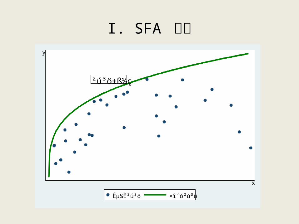
I. SFA 简介

²ú³ö±ß½ç

y

x

ʵ¼Ê²ú³ö ×î´ó²ú³ö

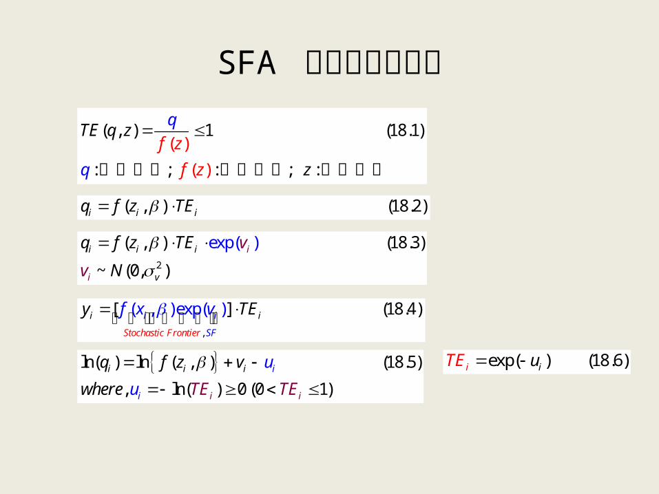
SFA 的模型设定思想

( , ) 1 (18.1)

: ; : ;

( )

( :)

f z

f

TE q

z

z

z

q

q

实际产出 理论产出 要素投入

( , ) (18.2)i i iq f z TE

2

( , ) (18.3)

~ (

exp )

0,

(

)

i i i i

i v

vq f z TE

Nv

,

( , )exp( )[ ] (18.4)Stochastic F

i i

SF

i

rontier

ivy TEf x

ln( ) ln ( , ) (18.5)

, ln( ) 0 (0 1)i i i i

i i i

q f z v

wh

u

er TE Te Eu

exp( ) (18.6)ii uTE

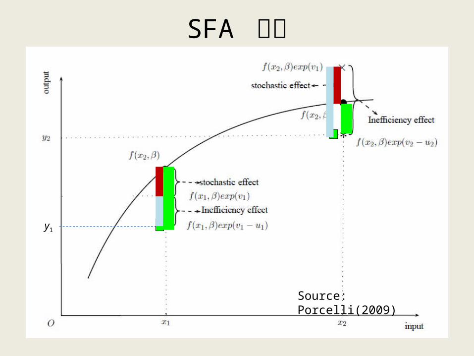
SFA 图示

y1

Source: Porcelli(2009)

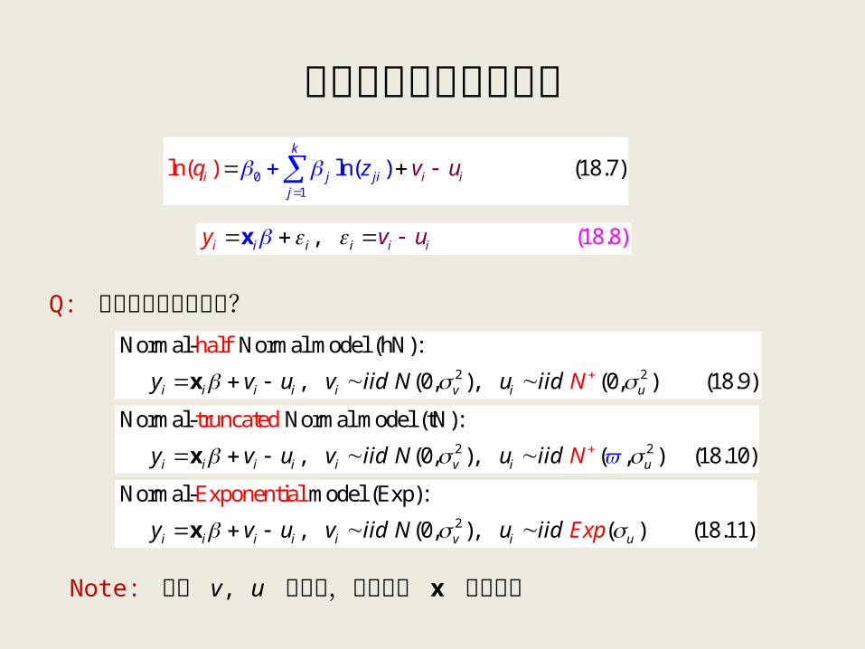
实证分析中的模型设定

01

lnln( ( ) (18. )) 7k

i ij

i j jiz v uq

Q: 两个干扰项如何处理？

2 2

Normal- Normal model (hN):

,

half

(0, ), (0, ) (18.9)i i i i i v i uy v u v i u id Nid N i x

2 2

Normal- Normal model (tN):

, (0, ), ( , ) (18.10)

truncated

i i i i i v i uy v u v iid N u iid N x

2

Normal- model (Exp):

, (0, ), ( ) (18.11)

Exponential

i i i i i v i uy v u v iid N u iid Exp x

, (18.8)i ii i i iy v u x

Note: 假设 v, u 不相关，且二者与 x 也不相关

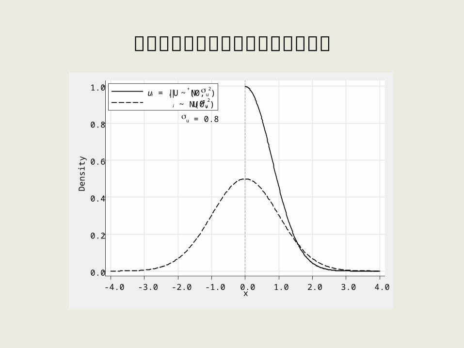
正态分布和半正态分布的密度函数图

u = 0.8

0.0

0.2

0.4

0.6

0.8

1.0D

ensi

ty

-4.0 -3.0 -2.0 -1.0 0.0 1.0 2.0 3.0 4.0x

ui = |Ui| ~ N+(0, u

2)

Ui ~ N(0, u2)

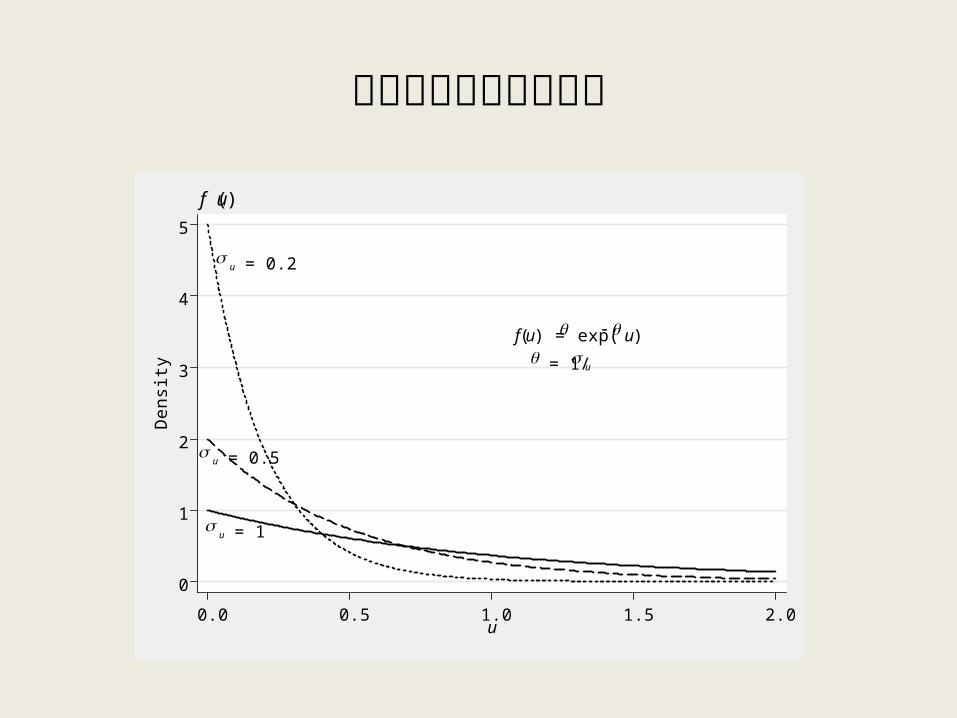
指数分布的密度函数图

u = 0.2

u = 0.5

u = 1

f(u) = exp( u)

= 1/ u

0

1

2

3

4

5

Den

sity

0.0 0.5 1.0 1.5 2.0u

f (u)

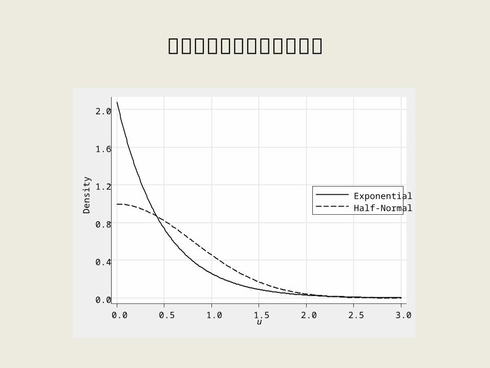
半正态分布和指数分布对比

0.0

0.4

0.8

1.2

1.6

2.0

Den

sity

0.0 0.5 1.0 1.5 2.0 2.5 3.0u

ExponentialHalf-Normal

效率的估计

• Jondrow, Lovell, Materov and Schmidt (1982) ， JLMS82

• Battese and Coelli (1988) ， BC88

(1

( ) + (18.25)

)

ii i i

ii i

i

E u

u

TE

E

21 1exp (18.26

exp

)1 2

i i

i

i

i

i

TE uE

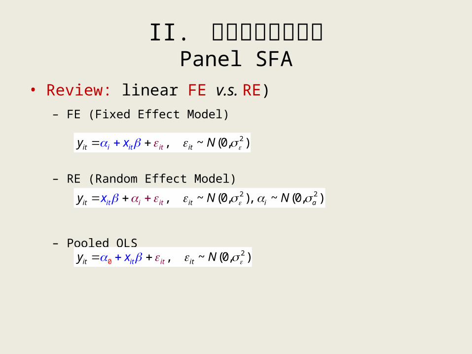
• Review: linear FE v.s. RE)– FE (Fixed Effect Model)

– RE (Random Effect Model)

– Pooled OLS

II. 面板随机边界模型Panel SFA

2, ~ (0, )itit iti ity Nx

2 2, ~ (0, ), ~ (0, )i iit it i ait ty N Nx

02, ~ (0, )itit it tixy N

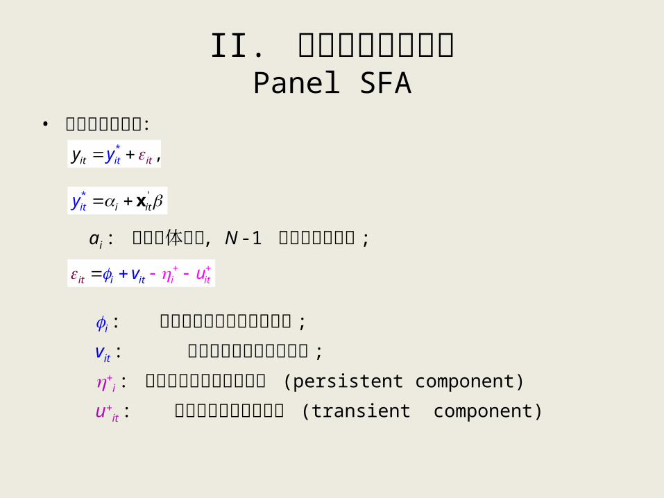
• 可能的通用模型：

ai : 公司个体效应 , N -1 个公司虚拟变量 ;

i : 不随时间变化的常规干扰项 ;

vit : 随时间变化的常规干扰项 ;

+i : 不随时间变化的无效率项 (persistent component)

u+it : 随时间变化的无效率项 (transient component)

II. 面板随机边界模型Panel SFA

* ,iti itty y

* 'ii tt iy x

i it i tt ii v u

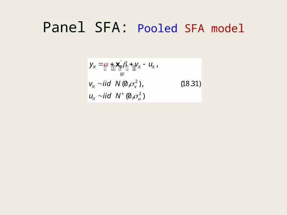
Panel SFA: Pooled SFA model

'

2

2

,

(0, ), (18.31)

(0, )

it it it it

S

it v

t

F

i u

y v u

v iid N

u iid N

x

• Pitt and Lee (1981), PL81

Panel SFA: 随机效应模型 (RE-SFA)效率不随时间变化

'

2

2

,

(0, ), (18.31)

(0, )

it it it

it v

i

i u

u

u

y v

v N

N

x

• Schmidt and Sickles (1984), SS84

• TE 的估计

Panel SFA: 固定效应模型 (FE-SFA)效率不随时间变化

' , (18.31) PL81,it it it iy v u x

' (18 ) E

,

F.34it it iti

i i

y v

u

x ， ，

(18.36)ˆ ˆmax ,

ˆ ˆˆ

M jj

i M iu

, (18 JLˆex MS8p ) 2.37i iTE u

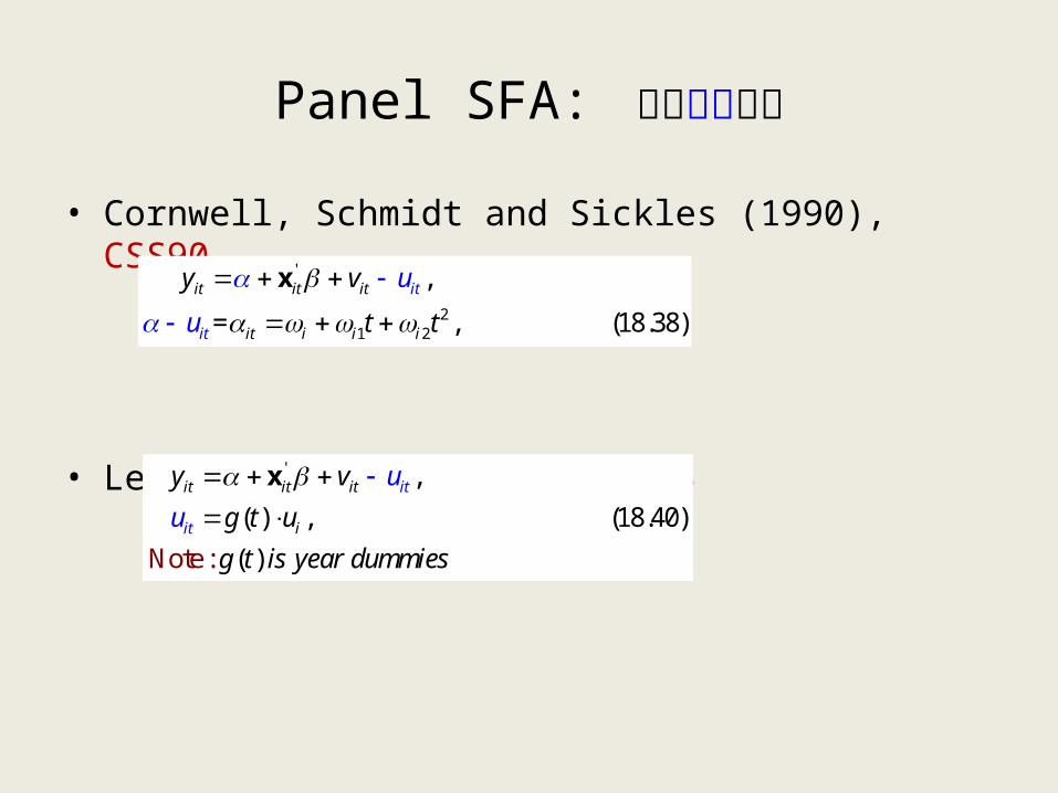
• Cornwell, Schmidt and Sickles (1990), CSS90

• Lee and Schmidt (1993), LS93

Panel SFA: 效率时变模型

'

21 2

,

= , (18.38)

it it it

it iit i i

ity v

t t

u

u

x

' ,

, (18.40

Note )

)

:

( )

(i

itit i t

it

t i u

u g t u

g t is year dumm

y

s

v

ie

x

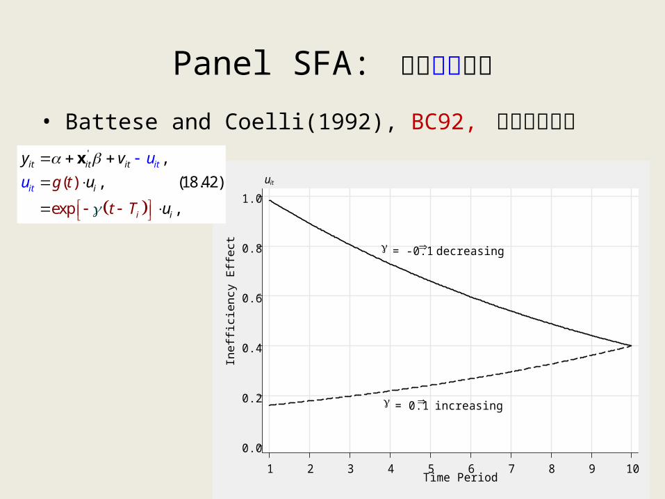
• Battese and Coelli(1992), BC92, 应用非常广泛

Panel SFA: 效率时变模型

= -0.1 decreasing

= 0.1 increasing

0.0

0.2

0.4

0.6

0.8

1.0

Inef

fici

ency

Eff

ect

1 2 3 4 5 6 7 8 9 10Time Period

uit

'

( )

exp

,

(18.42, )

,

it

i

it it i

i

i

i

t

t

y v u

u g

t T

u

u

t

x

• Greene 难题 (Greene Problem)

– True-Model:

– Estimate-Model:

– Implications: • TE 的估计值将是有偏的• 把那些个体异质性 ( 公司文化 , CEO 特征等 ) 影响产出的因素都归为

“无效率项”了

Panel SFA: True FE SFA

' (18.43)it it it it

inEffSF

iy v u x

'

0 (18.44)it it it

inEffSF

ity uv x

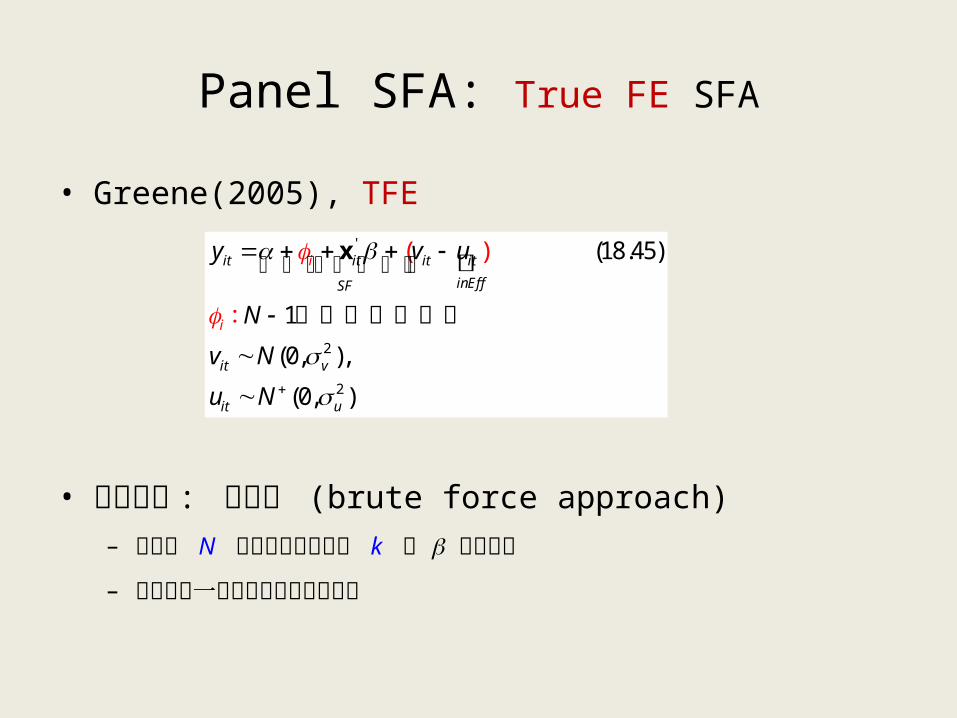
• Greene(2005), TFE

• 估计方法 : 蛮力法 (brute force approach)– 直接估 N 个公司虚拟变量和 k 个 参数即可

– 需要采用一些特殊的数值计算技巧

Panel SFA: True FE SFA

'

2

2

(18.45)

1

(0, ),

( )

(0, )

i

i

it it it it

inEffSF

it v

it u

y v u

N

v N

u N

x

个公司虚拟变量：

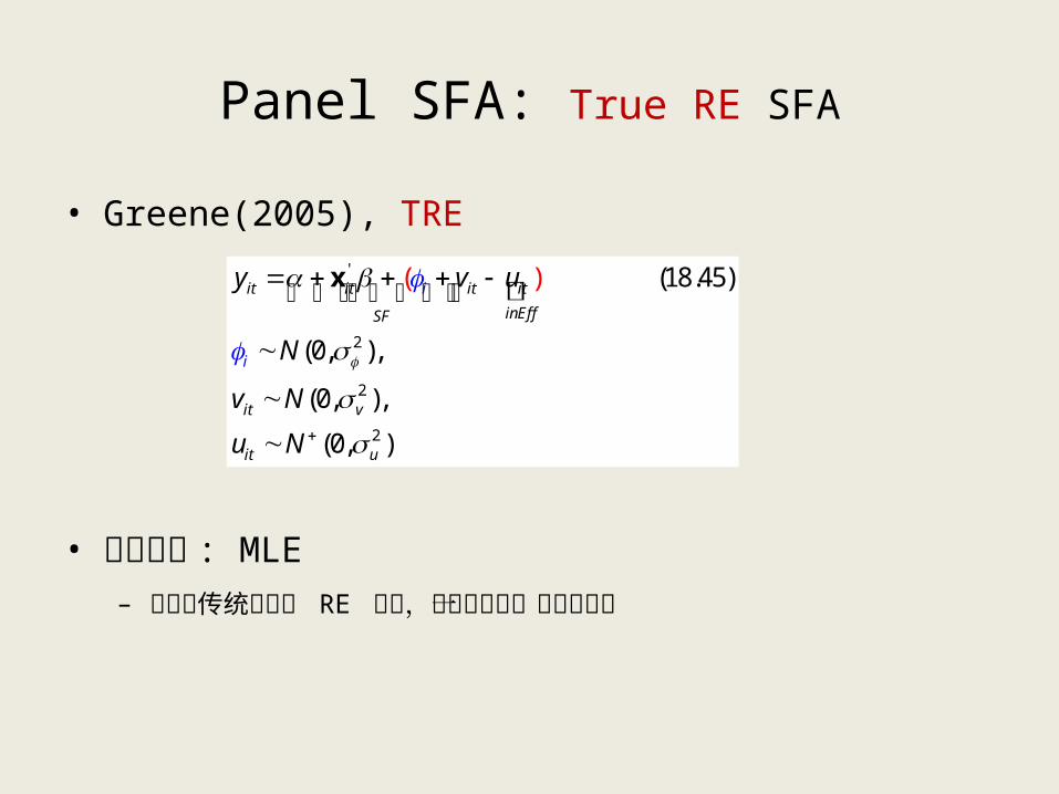
• Greene(2005), TRE

• 估计方法 : MLE– 相对于传统的线性 RE 模型，只是增加了一个参数而已

Panel SFA: True RE SFA

'

2

2

2

(18.45)

(0, ),

(0, )

)

,

(0,

(

)

i

i

it it it it

inEffSF

it v

it u

y v u

N

v N

u N

x

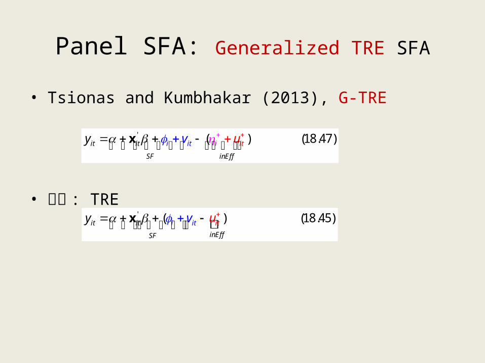
• Tsionas and Kumbhakar (2013), G-TRE

• 对比 : TRE

Panel SFA: Generalized TRE SFA

' ( ) (18.47)it it

SF

iti it

inE

i

ff

y uv x

' ( ) (18.45)it it

inEffSF

i t iti uy v x

• Wang and Ho (2010), Scaling-TFE

• git： scaling function, 是公司特征变量 (zit) 的函数– git ：可以使非效率具有异质性；– git ：缩放性质使得我们可以用 FD 或组内去心去除个体效应 i

Panel SFA: Scaling-TFE SFA

'

2

(18.52)

( )

( , )

it it it

i

i

it

it

i u

t

it

t

i i

g

y v u

zg

u

u u

f

N

x

，，，

，

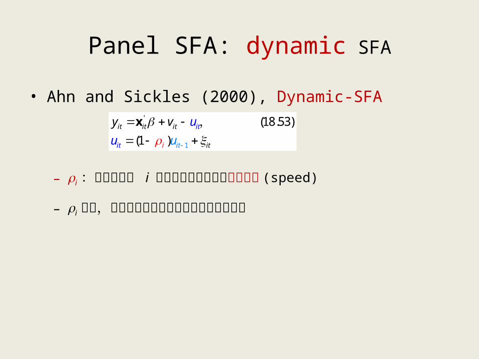
• Ahn and Sickles (2000), Dynamic-SFA

– i ：用于衡量第 i 家公司对非效率项的调整能力 (speed)

– i 越大，表明公司克服其非效率行为的能力越强

Panel SFA: dynamic SFA

'

1

(18.53)

(1 ) ii

it itit it

it tti

u

u

y v

u

x ，

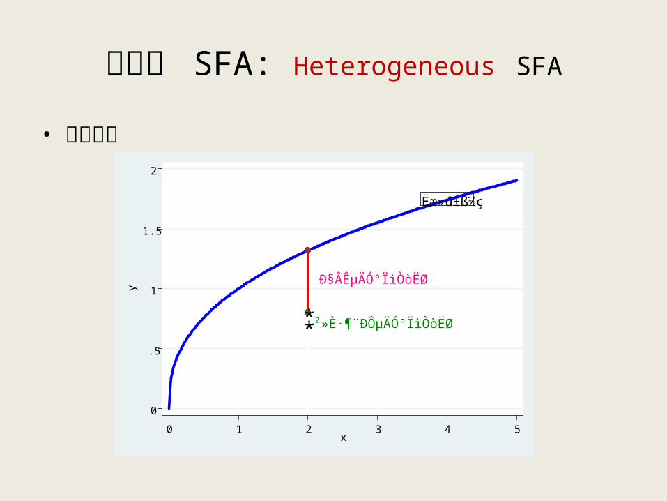
异质性 SFA: Heterogeneous SFA

• 基本思想

Ëæ»ú±ß½ç

ЧÂʵÄÓ°ÏìÒòËØ

**²»È·¶¨ÐÔµÄÓ°ÏìÒòËØ

0

.5

1

1.5

2

y

0 1 2 3 4 5x

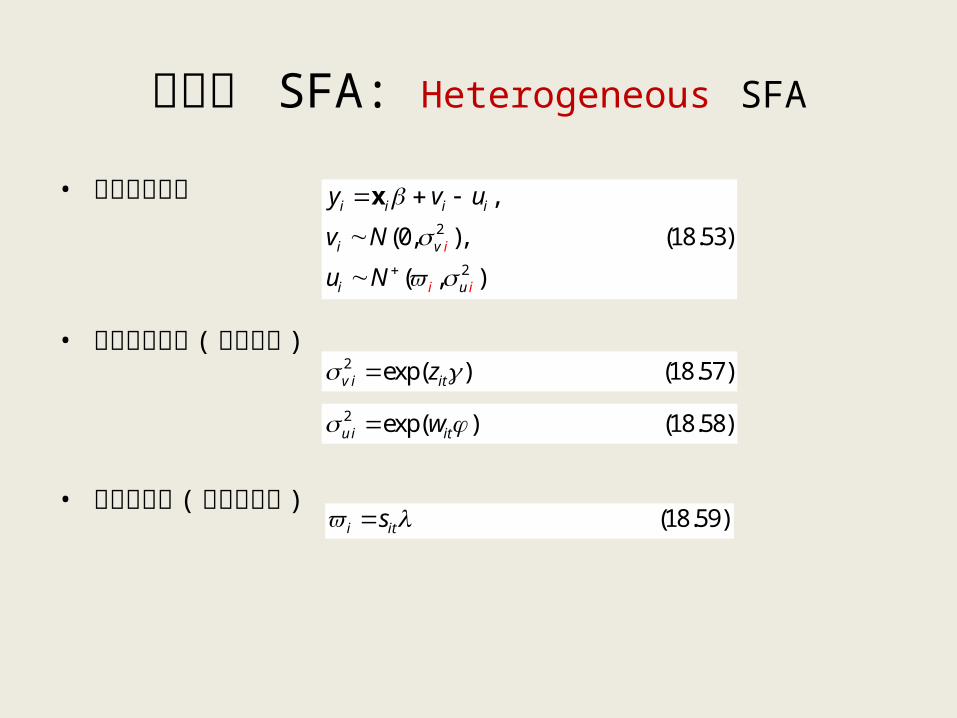
• 模型设定思想

• 异方差的设定 ( 不确定性 )

• 均值的设定 ( 无效率水平 )

异质性 SFA: Heterogeneous SFA

2

2

,

(0, ), (18.53)

( , )

i

i i i i

i v

i ui i

y v u

v N

u N

x

2 exp( ) (18.57)v i itz

2 exp( ) (18.58)u i itw

(18.59)i its

• 基本思想

双边随机边界模型 : two-tier SFA

Ëæ»ú±ß½ç

*Over

* Under

0

.5

1

1.5

2

y

0 1 2 3 4 5x

• 模型设定

• 效率的估计

双边随机边界模型 : two-tier SFA

2

2

2

(18.6

( )

~ . . . (0, )

~ . . . ( , )

~ . . . ( ,

0)

)

i i i

SF inEff

i v

w

i

w

i

i u

i

u

y v

v i i d N

i i d Exp

i i d E

w

u

w

p

u

x

x

(18.66)% -invest (1 | )

% -invest (1 | )i

ii

i

w

uunde

o E e

er E

ver

Thanks

New Course: http://baoming.pinggu.org/Default.aspx?id=93

References 1• Aigner, D., C. Lovell, P. Schmidt, 1977, Formulation and estimation of

stochastic frontier production function models, Journal of Econometrics, 6 (1): 21-37.

• Arellano, M., S. Bond, 1991, Some tests of specification for panel data: Monte carlo evidence and an application to employment equations, Review of Economic Studies, 58 (2): 277-297.

• Arellano, M., O. Bover, 1995, Another look at the instrumental variable estimation of error-components models, Journal of Econometrics, 68 (1): 29-51.

• Battese, G., T. Coelli, 1992, Frontier production functions, technical efficiency and panel data: With application to paddy farmers in india, Journal of Productivity Analysis, 3 (1): 153-169.

• Battese, G. E., T. J. Coelli, 1988, Prediction of firm-level technical efficiencies with a generalized frontier production function and panel data, Journal of Econometrics, 38 (3): 387-399.

• Battese, G. E., T. J. Coelli, 1995, A model for technical inefficiency effects in a stochastic frontier production function for panel data, Empirical Economics, 20 (2): 325-332.

• Belotti, F., S. Daidone, G. Ilardi, V. Atella, 2013, Stochastic frontier analysis using stata, Stata Journal: forthcoming.

• Chang, S. K., Y. Y. Chen, H. J. Wang, 2012, A bayesian estimator for stochastic frontier models with errors in variables, Journal of Productivity Analysis, 38 (1): 1-9.

• Chen, N.-K., Y.-Y. Chen, H.-J. Wang, 2011, Asset prices and capital investment–a panel stochastic frontier approach, Working Paper.

References 2• Coelli, T., D. Prasada Rao, G. E. Battese. An introduction to efficiency and

productivity analysis[M]. Boston: Kluwer Academic Publishers 1998.• Colombi, R., G. Martini, G. Vittadini, 2011, A stochastic frontier model with

short-run and long-run inefficiency, Working Paper, Department of Economics and Technology Management, Universita di Bergamo, Italy.

• Emvalomatis, G., 2012, Adjustment and unobserved heterogeneity in dynamic stochastic frontier models, Journal of Productivity Analysis, 37 (1): 7-16.

• Feng, G., A. Serletis, 2009, Efficiency and productivity of the us banking industry, 1998–2005: Evidence from the fourier cost function satisfying global regularity conditions, Journal of Applied Econometrics, 24 (1): 105-138.

• Fried, H. O., C. Lovell, S. S. Schmidt. 2008, Efficiency and productivity[C], in H. O. Fried, C. Lovell,S. S. Schmidt eds, The measurement of productive efficiency and productivity change (Oxford University Press, New York) 3-92.

• Greene, W., 2005a, Fixed and random effects in stochastic frontier models, Journal of Productivity Analysis, 23 (1): 7-32.

• Greene, W., 2005b, Reconsidering heterogeneity in panel data estimators of the stochastic frontier model, Journal of Econometrics, 126 (2): 269-303.

• Greene, W., 2008, The econometric approach to efficiency analysis, The Measurement of Productive Efficiency and Productivity Change, 1 (5): 92-251.

References 3• Habib, M., A. Ljungqvist, 2005, Firm value and managerial incentives: A

stochastic frontier approach, Journal of Business, 78 (6): 2053-2094.• Hadri, K., 1999, Estimation of a doubly heteroscedastic stochastic frontier

cost function, Journal of Business & Economic Statistics, 17 (3): 359-363.• Huang, C. J., J.-T. Liu, 1994, Estimation of a non-neutral stochastic frontier

production function, Journal of Productivity Analysis, 5 (2): 171-180.• Jondrow, J., K. Lovell, I. Materov, P. Schmidt, 1982, On the estimation of

technical inefficiency in the stochastic frontier production function model, Journal of Econometrics, 19 (2-3): 233-238.

• Koutsomanoli-Filippaki, A., E. C. Mamatzakis, 2010, Estimating the speed of adjustment of european banking efficiency under a quadratic loss function, Economic Modelling, 27 (1): 1-11.

• Kumbhakar, S., F. Christopher, 2009, The effects of bargaining on market outcomes: Evidence from buyer and seller specific estimates, Journal of Productivity Analysis, 31 (1): 1-14.

• Kumbhakar, S., G. Lien, J. B. Hardaker, 2012a, Technical efficiency in competing panel data models: A study of norwegian grain farming, Journal of Productivity Analysis: 1-17.

References 4• Kumbhakar, S., C. Lovell. Stochastic frontier analysis[M]. Cambridge:

Cambridge University Press, 2000.• Kumbhakar, S., R. Ortega-Argilés, L. Potters, M. Vivarelli,P. Voigt, 2012b,

Corporate r&d and firm efficiency: Evidence from europe’s top r&d investors, Journal of Productivity Analysis, 37 (2): 125-140.

• Kumbhakar, S. C., 1990, Production frontiers, panel data, and time-varying technical inefficiency, Journal of Econometrics, 46 (1): 201-211.

• Kumbhakar, S. C., S. Ghosh, J. T. McGuckin, 1991, A generalized production frontier approach for estimating determinants of inefficiency in us dairy farms, Journal of Business & Economic Statistics, 9 (3): 279-286.

• Kumbhakar, S. C., C. F. Parmeter, E. G. Tsionas, 2013, A zero inefficiency stochastic frontier model, Journal of Econometrics, 172 (1): 66-76.

• Kumbhakar, S. C., E. G. Tsionas, 2011, Some recent developments in efficiency measurement in stochastic frontier models, Journal of Probability and Statistics, 2011: forthcoming.

• Lai, H.-p., C. J. Huang, 2011, Maximum likelihood estimation of seemingly unrelated stochastic frontier regressions, Journal of Productivity Analysis: 1-14.

References 5

• Lee, Y. H., P. Schmidt. 1993, A production frontier model with flexible temporal variation in technical efficiency[C], in H. Fried, C. Lovell,S. Schmidt eds, The measurement of productive efficiency: Techniques and applications (Oxford University Press, Oxford, UK) 237-255.

• Lian, Y., C.-F. Chung, 2008, Are chinese listed firms over-investing?, SSRN working paper, Available at SSRN: http://ssrn.com/abstract=1296462.

• Meeusen, W., J. Van den Broeck, 1977, Efficiency estimation from cobb-douglas production functions with composed error, International Economic Review, 18 (2): 435-444.

• Peyrache, A., A. N. Rambaldi, 2012, A state-space stochastic frontier panel data model, working Paper.

• Pitt, M. M., L.-F. Lee, 1981, The measurement and sources of technical inefficiency in the indonesian weaving industry, Journal of Development Economics, 9 (1): 43-64.

• Tsionas, E. G., S. C. Kumbhakar, 2013, Firm-heterogeneity, persistent and transient technical inefficiency:A generalized true random effects model, Journal of Applied Econometrics: forthcoming.

References 6• Wang, E. C., 2007, R&d efficiency and economic performance: A cross-

country analysis using the stochastic frontier approach, Journal of Policy Modeling, 29 (2): 345-360.

• Wang, H., 2003, A stochastic frontier analysis of financing constraints on investment: The case of financial liberalization in taiwan, Journal of Business and Economic Statistics, 21 (3): 406-419.

• Wang, H. J., C. W. Ho, 2010, Estimating fixed-effect panel stochastic frontier models by model transformation, Journal of Econometrics, 157 (2): 286-296.

• Yélou, C., B. Larue, K. C. Tran, 2010, Threshold effects in panel data stochastic frontier models of dairy production in canada, Economic Modelling, 27 (3): 641-647.

• 白俊红 , 江可申 , 李婧 , 2009, 应用随机前沿模型评测中国区域研发创新效率 , 管理世界 , (10): 51-61.

• 林伯强 , 杜克锐 , 2013, 要素市场扭曲对能源效率的影响 , 经济研究 , (9): 125-136.• 刘海洋 , 逯宇铎 , 陈德湖 , 2013, 中国国有企业的国际议价能力估算 , 统计研究 , (5):

47-53.• 卢洪友 , 连玉君 , 卢盛峰 , 2011, 中国医疗服务市场中的信息不对称程度测算 , 经济研

究 , (4): 94-106.

What’s More http://baoming.pinggu.org/Default.aspx?id=93