1 15.053 thursday, april 25 nonlinear programming theory separable programming handouts: lecture...
TRANSCRIPT

1
15.053 Thursday, April 25
• Nonlinear Programming Theory
• Separable programming
Handouts: Lecture Notes

2
Difficulties of NLP Models
LinearProgram:
NonlinearPrograms:

3
Graphical Analysis of Non-linear programsin two dimensions: An example
• Minimize
• subject to (x - 8)2 + (y - 9)2 ≤ 49 x ≥2 x ≤13 x + y ≤24

4
Where is the optimal solution?
Note: the optimalsolution is not at acorner point.It is where theisocontour first hitsthe feasible region.
5
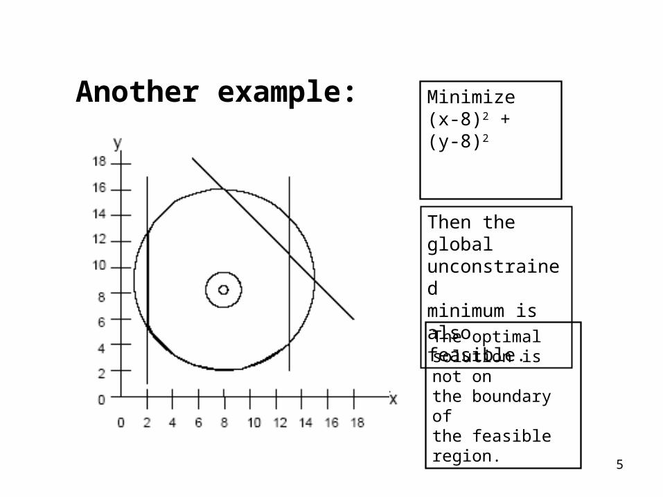
Another example: Minimize(x-8)2 + (y-8)2
Then the globalunconstrainedminimum is alsofeasible.
The optimalsolution is not onthe boundary ofthe feasible region.

6
Local vs. Global Optima
Def’n: Let x be a feasible solution, then
– x is a global max if f(x) ≥ f(y) for every feasible y.
– x is a local max if f(x) ≥ f(y) for every feasible y sufficiently close to x (i.e., xj-ε ≤ yj ≤ xj+ ε for all j and some small ε).
There may be several locally optimal solutions.

7
When is a locally optimal solutionalso globally optimal?
• We are minimizing. The objective function is convex. The feasible region is convex.

8
Convexity and Extreme Points
We say that a set S is convex, if for everytwo points x and y in S, and for every realnumber λ in [0,1], λx + (1-λ)y ε S.
The feasible region of a linear program is convex.
We say that an element w ε S is anextreme point (vertex, corner point), if wis not the midpoint of any line segmentcontained in S.

9
Recognizing convex feasible regions
• If all constraints are linear, then the feasible region is convex
• The intersection of convex regions is convex
• If for all feasible x and y, the midpoint of x and y is feasible, then the region is convex (except in totally non-realistic examples. )

10
Which are convex?

11
Convex FunctionsConvex Functions: f( y + (1- )z) f(y) + (1- )f(z)for every y and z and for 0. e.g., f((y+z)/2) f(y)/2 + f(z)/2
We say “strict” convexity if signis “<” for 0.
Line joining any pointsis above the curve

12
Convex FunctionsConvex Functions: f( y + (1- )z) ≥ f(y) + (1- )f(z)for every y and z and for 0. e.g., f((y+z)/2) ≥ f(y)/2 + f(z)/2
We say “strict” convexity if signis “<” for 0.
Line joining any pointsis above the curve

13
Classify as convex or concave or bothor neither.

14
What functions are convex?
• f(x) = 4x + 7 all linear functions• f(x) = 4x2 – 13 some quadratic functions• f(x) = ex
• f(x) = 1/x for x > 0• f(x) = |x|• f(x) = - ln(x) for x > 0
Sufficient condition: f”(x) > 0 for all x.

15
What functions are convex?
• If f(x) is convex, and g(x) is convex. Then so is h(x) = a f(x) + b g(x) for a>0, b>0.
• If y = f(x) is convex, then {(x,y) : f(x) ≤ y} is a convex set

16
Local Maximum (Minimum)Property
• A local max of a concave function on a convex feasible region is also a global max.• A local min of a convex function on a convex feasible region is also a global min.• Strict convexity or concavity implies that the global optimum is unique.• Given this, we can exactly solve: – Maximization Problems with a concave objective function and linear constraints – Minimization Problems with a convex objective function and linear constraints

17
Which are convex feasible regions?
(x, y) : y ≤ x2 + 2
(x, y) : y ≥ x2 + 2
(x,y) : y = x2 + 2

18
More on local optimality
• The techniques for non-linear optimization minimization usually find local optima.• This is useful when a locally optimal solution is a globally optimal solution• It is not so useful in many situations.
• Conclusion: if you solve an NLP, try to find out how good the local optimal solutions are.

19
Solving NLP’s by Excel Solver

20
Finding a local optimal for a singlevariable NLP
Solving NLP's with One Variable:
max f(θ)s.t. a ≤ θ ≤ b
Optimal solution is either a boundary point or satisfies f′(θ∗) = 0 and f ″(θ∗) < 0.

21
Solving Single Variable NLP (contd.)
If f(θ) is concave (or simply unimodal) and differentiable
max f(θ)s.t. a ≤ θ ≤ b
Bisection (or Bolzano) Search:
• Step 1. Begin with the region of uncertainty for θ as [a,b]. Evaluate f ′ (θ) at the midpoint θΜ =(a+b)/2.
• Step 2. If f ′ (θΜ) > 0, then eliminate the interval up to θΜ.If f′(θΜ) < 0, then eliminate the interval beyond θΜ.
• Step 3. Evaluate f′(θ) at the midpoint of the newinterval. Return to Step 2 until the interval of uncertaintyis sufficiently small.

22
Unimodal Functions
• A single variable function f is unimodal if there is at most one local maximum (or at most one local
minimum) .
23
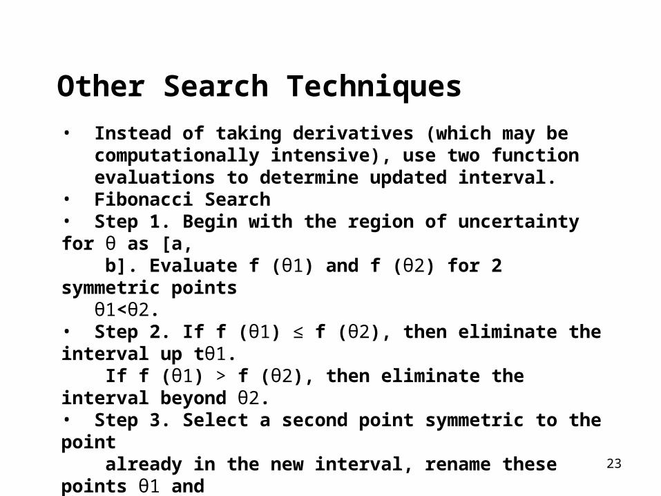
Other Search Techniques
• Instead of taking derivatives (which may be computationally intensive), use two function evaluations to determine updated interval.• Fibonacci Search• Step 1. Begin with the region of uncertainty for θ as [a, b]. Evaluate f (θ1) and f (θ2) for 2 symmetric points θ1<θ2.• Step 2. If f (θ1) ≤ f (θ2), then eliminate the interval up tθ1. If f (θ1) > f (θ2), then eliminate the interval beyond θ2.• Step 3. Select a second point symmetric to the point already in the new interval, rename these points θ1 and θ2 such that θ1<θ2 and evaluate f (θ1) and f (θ2). Return to Step 2 until the interval is sufficiently small.

24
On Fibonacci search
1, 1, 2, 3, 5, 8, 13, 21, 34At iteration 1, the length of the search interval is the kth fibonacci number for some kAt iteration j, the length of the search interval is the k-j+1 fibonacci number.The technique converges to the optimal when the function is unimodal.

25
Finding a local maximum usingFibonacci Search.
Length of search
interval
Where the maximum may be
26
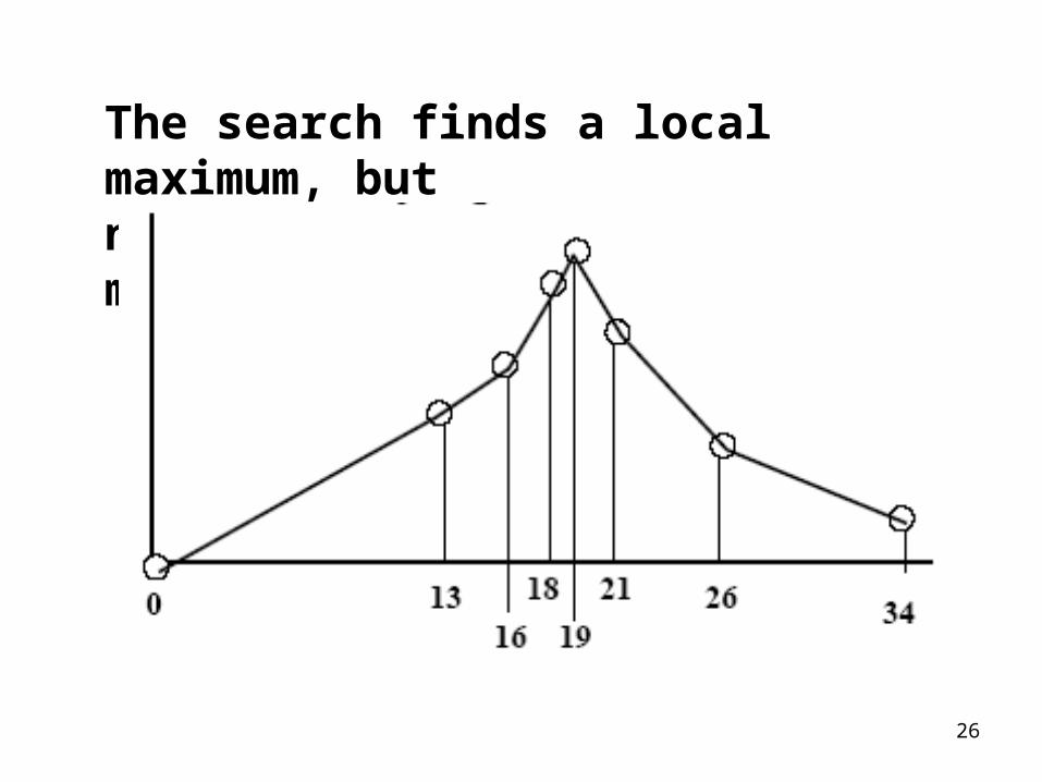
The search finds a local maximum, butnot necessarily a global maximum.
27
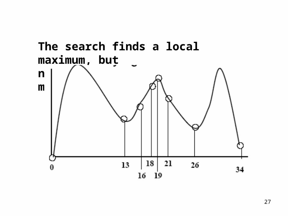
The search finds a local maximum, butnot necessarily a global maximum.

28
Number of function evaluations inFibonacci Search
• As new point is chosen symmetrically, the length lk of successive search intervals is given by: lk= lk+1 + lk+2 .• Solving for these lengths given a final interval length of 1, ln = 1, gives the Fibonacci numbers: 1, 2, 3, 5, 8, 13, 21, 34,…• Thus, if the initial interval has length 34, it takes 8 function calculations to reduce the interval length to 1.
• Remark: if the function is convex or unimodal, then fibonacci search converges to the global maximum

29
Separable Programming
• Separable programs have the form:
Max
st
Each variable xj appears separately, one ineach function gij and one in each function fj inthe objective.
Each non-linear function is of a single variable.

30
Examples of SeparablePrograms
f(x1,x2) = x1(30-x1)+x2(35-x2)-2x12-3x2
2
f(x1,x2) = x15 + -18e-x2-4x2
3
x1
f(x1,x2,x2) = lnx15-sinx2-x3e-x3)+7x1
-4

31
Approximating a non-linear functionwith a piecewise linear function.
• Aspect 1. Choosing the approximation.• Aspect 2. When is the piecewise linear approximation a linear program in disguise?

32
Approximating a non-linearfunction of 1 variable

33
Approximating a non-linear functionof 1 variable: the λ method
Choosedifferentvalues of x toapproximatethe x-axis
Approximateusingpiecewiselinearsegments

34
More on the method
Suppose that for –3 ≤ x ≤ -1,
we represent x hasλ1 (-3) +λ2 (-1)
whereλ1 +λ2 = 1 andλ1,λ2 ≥ 0
Then we approximate f(x) as
λ1 (-20) +λ2 (-7 1/3)
a1 = -3, f(a1) = -20
a2 = -1 f(a2) = -7 1/3

35
More on the method
a2 = -1, f(a2) = -7 1 /3
a3 = 1 f(a3) = -2 2/3
Suppose that for –1 ≤ x ≤ 1,
we represent x hasλ2 (-3) +λ3 (-1)whereλ2 +λ3 = 1 andλ2,λ3 ≥ 0
How do weapproximate f( ) inthis interval?
What if –3 ≤ x ≤ 1?

36
Almost the method
Original problem:
min x3/3 + 2x – 5 + more terms
s.t. -3 ≤ x ≤ 3 + many more constraints
a1 = -3; a2 = - 1; a3 = 1; a4 = 3f(a1) = -20; f(a2) = -7 1/3; f(a3) = -2 2/3; f(a4) = 4
Approximated problem:
minλ1f(a1) +λ2f(a2) +λ3f(a3) +λ4f(a4)
more linear terms
s.t. λ1 + λ2 + λ3 + λ4= 1 ; λ ≥ 0
+ many more constraints

37
Why the approximation is incorrect
Approximated problem:
minλ1f(a1) +λ2f(a2) +λ3f(a3) +λ4f(a4)
more linear terms
s.t. λ1+λ2 +λ3+λ4 = 1 ; λ ≥ 0Considerλ1= 1/2 ;λ2=0 ;λ3=1/2 ;λ4 = 0;
The method givesthe correctapproximation ifonly twoconsecutiveλs arepositive.

38
Adjacency Condition
1. At most two weights (λs) are positive2. If exactly two weights (λs) are positive, then they are λj and λj+1 for some j3. The same condition applies to every approximated function.

39
Approximating a non-linear objectivefunction for a minimization NLP. original problem: minimize {f(y): y ∈P} Suppose that y = Σjjaj , where Σjj = 1 and >= 0 . Approximate f(y). minimize {Σjjf(aj): Σjjaj∈P}
• Note: when given a choice of representing y in alternative ways, the LP will choose one that leads to the least objective value for the approximation.

40
For minimizing a convex function, the-method automatically satisfies theadditional adjacency property.
min Z =λ1f(a1) +λ2f(a2) +λ3f(a3) +λ4f(a4)+λ5f(a5) s.t. λ1 + λ2 + λ3 + λ4 +λ5 = 1; ≥0 + adjacency condition + other constraints

41
Feasible approximated objective functions without the adjacency conditions
min Z =λ1f(a1) +λ2f(a2) +λ3f(a3) +λ4f(a4)+λ5f(a5) s.t. λ1 + λ2 + λ3 + λ4 +λ5 = 1; ≥0 + other constraints

42
But a minimum in this case always occurson the piecewise linear curve.
min Z =λ1f(a1) +λ2f(a2) +λ3f(a3) +λ4f(a4)+λ5f(a5) s.t. λ1 + λ2 + λ3 + λ4 +λ5 = 1; ≥0 + other constraints

43
Separable Programming (in the case oflinear constraints)
• Begin with an NLP:
• Transform to Separable:
• Approximate using the Method:
Max f ( )xs.t. Dx d x 0
Max ∑fj (xj) s.t. Dx d x
0
n
j=1

44
Approximation
• Re-express in terms of variables:
If the original problem is concave, then you can drop theadjacency conditions (they are automatically satisfied.)
and the adjacency conditions

45
How can one construct separable functions?
Term Substitution Constraints Restriction
None
None
None

46
Transformation Examples
Ex : (x1 + x2 + x3)6
Substitute y6 and let y = x1 + x2 + x3
x1x22
1+ x3
Ex : let y1and let y2
and add the constraint

47
NLP Summary
• Convex and Concave functions as well as convex sets are important properties• Bolzano and Fibonacci search techniques – used to solve single variable unimodal functions• Separable Programming – nonlinear objective and nonlinear constraints that are separable – General approximation technique