1

Quantity Theory of Quantity Theory of MoneyMoney

VelocityVelocityP P Y Y

VV = =MM

Equation of Exchange Equation of Exchange M M V V = = P P Y Y

Quantity Theory of MoneyQuantity Theory of Money

1. Irving Fisher’s view: 1. Irving Fisher’s view: VV is fairly constant is fairly constant2. Equation of exchange no longer identity2. Equation of exchange no longer identity3. Nominal income, 3. Nominal income, PYPY, determined by , determined by MM4. Classicals assume 4. Classicals assume YY is determined by real factors, is determined by real factors, not monetarynot monetary5.5. P P determined by determined by MM

Quantity Theory of Money DemandQuantity Theory of Money Demand

1 1 MM = = PY PY VV

MMdd = = kk PYPY

Implication:Implication: interest rates not important to interest rates not important to MMdd

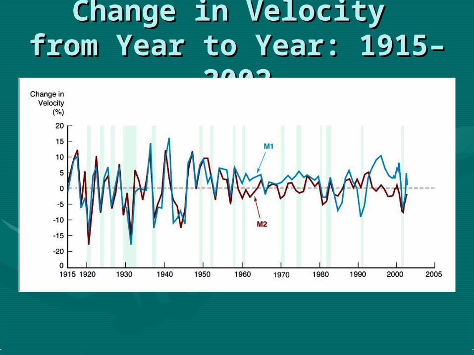
Change in Velocity Change in Velocity from Year to Year: 1915–from Year to Year: 1915–

20022002

Cambridge ApproachCambridge Approach

Is velocity constant?Is velocity constant?1.1. Classicals thought Classicals thought VV

constant because didn’t have constant because didn’t have good datagood data

2.2. After Great Depression, After Great Depression, economists realized velocity economists realized velocity far from constantfar from constant

Keynes’s Liquidity Keynes’s Liquidity Preference TheoryPreference Theory

3 Motives3 Motives

1.1. Transactions motive—related to Transactions motive—related to YY

2.2. Precautionary motive—constantPrecautionary motive—constant

3.3. Speculative motiveSpeculative motive

A. related to A. related to WW and and YY

B. negatively related to B. negatively related to ii

Liquidity PreferenceLiquidity Preference

MMdd

= f(= f(i, Yi, Y)) PP – + – +

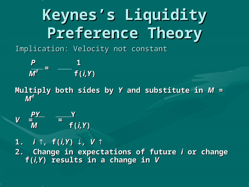
Keynes’s Liquidity Keynes’s Liquidity Preference TheoryPreference Theory

Implication: Velocity not constantImplication: Velocity not constant

PP 1 1 == MMdd f( f(i,Yi,Y))

Multiply both sides by Multiply both sides by YY and substitute in and substitute in MM = = MMdd

PYPY Y YVV = = = =

MM f( f(i,Yi,Y))

1. 1. ii , f(, f(i,Yi,Y) ) , , VV 2. Change in expectations of future 2. Change in expectations of future ii or change or change

f(f(i,Yi,Y) results in a change in ) results in a change in VV

6

Determination of OutputDetermination of OutputKeynesian Keynesian IS-LMIS-LM Model assumes price level is fixed Model assumes price level is fixed

Aggregate DemandAggregate Demand

YYadad = = CC + + II + + GG + + NXNX

EquilibriumEquilibrium

YY = = YYadad

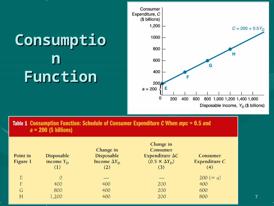
Consumption FunctionConsumption Function

CC = = aa + ( + (mpcmpc YYDD))

InvestmentInvestment

1.1. Fixed investmentFixed investment

2.2. Inventory investmentInventory investment

Only planned investment is included in Only planned investment is included in YYadad

7

ConsumptiConsumption on

FunctionFunction

8

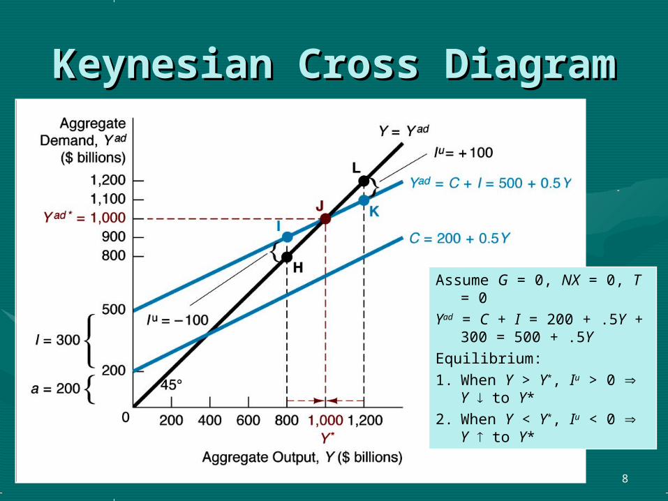
Keynesian Cross Keynesian Cross DiagramDiagram

Assume G = 0, NX = 0, T = 0

Yad = C + I = 200 + .5Y + 300 = 500 + .5Y

Equilibrium:1. When Y > Y*, Iu > 0 Y

to Y*2. When Y < Y*, Iu < 0 Y

to Y*

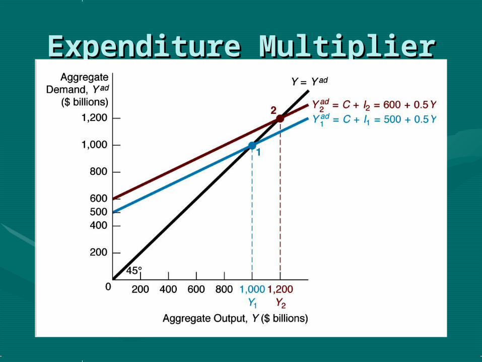
Expenditure MultiplierExpenditure Multiplier

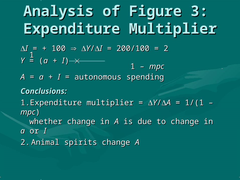
Analysis of Figure 3: Analysis of Figure 3: Expenditure MultiplierExpenditure Multiplier

II = + 100 = + 100 YY//II = 200/100 = 2 = 200/100 = 211

YY = ( = (aa + + II) ) 1 – 1 – mpcmpcAA = = aa + + II = autonomous spending = autonomous spending

Conclusions:Conclusions:

1.1. Expenditure multiplier = Expenditure multiplier = YY//AA = 1/(1 – = 1/(1 – mpcmpc))whether change in whether change in AA is due to change in is due to change in aa or or II

2.2. Animal spirits change Animal spirits change AA

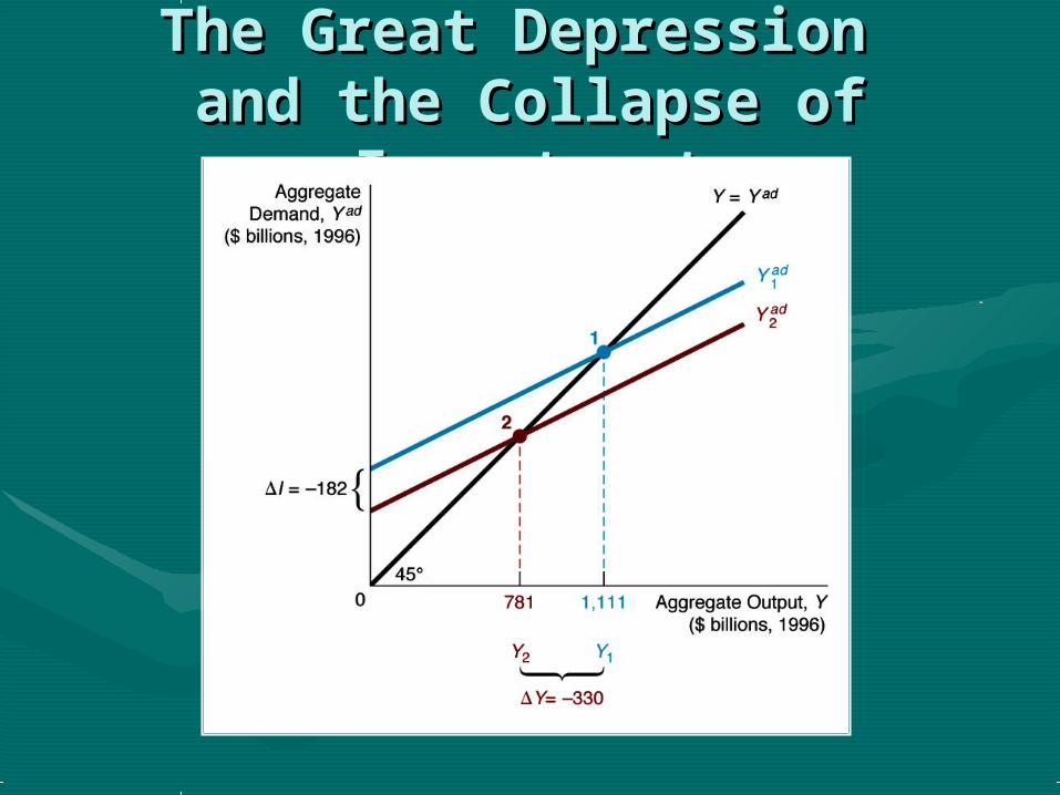
The Great Depression The Great Depression and the Collapse of and the Collapse of

InvestmentInvestment

Role of GovernmentRole of Government

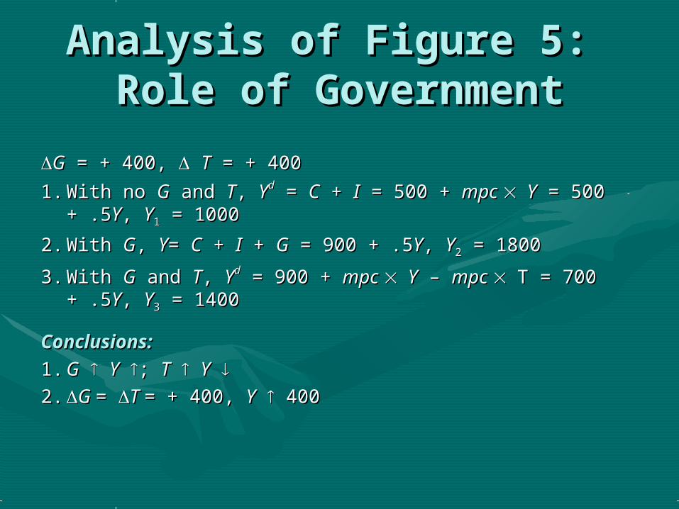
Analysis of Figure 5: Analysis of Figure 5: Role of GovernmentRole of Government

GG = + 400, = + 400, TT = + 400 = + 400

1.1. With no With no GG and and TT, , YYdd = = CC + + II = 500 + = 500 + mpc mpc YY = 500 + .5 = 500 + .5YY, , YY11 = 1000 = 1000

2.2. With With GG, , YY= = CC + + II + + GG = 900 + .5 = 900 + .5YY, , YY22 = 1800 = 1800

3.3. With With GG and and TT, , YYdd = 900 + = 900 + mpc mpc YY – – mpc mpc T = 700 + .5T = 700 + .5YY, , YY33 = 1400 = 1400

Conclusions:Conclusions:

1.1. GG YY ; ; TT YY 2.2. G G = = T T = + 400, = + 400, YY 400 400

Role of International Role of International TradeTrade

NX = +100,Y/NX = 200/100 = 2

= 1/(1 – mpc) = 1/(1 – .5)

Summary: Summary: Factors Factors

that that Affect Affect YY

16

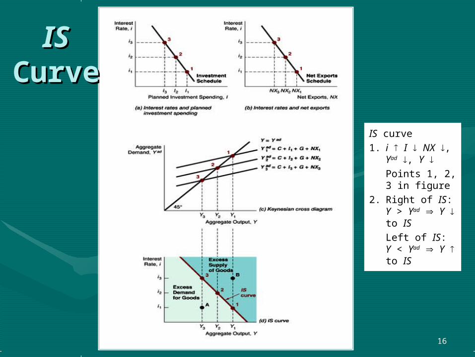
ISIS CurveCurve

IS curve1. i I NX ,

Yad , Y Points 1, 2, 3 in figure

2. Right of IS: Y > Yad Y to ISLeft of IS: Y < Yad Y to IS

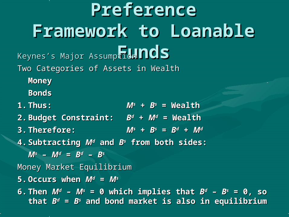
Relation of Liquidity Relation of Liquidity PreferencePreference

Framework to Loanable Framework to Loanable FundsFundsKeynes’s Major AssumptionKeynes’s Major Assumption

Two Categories of Assets in WealthTwo Categories of Assets in Wealth

MoneyMoney

BondsBonds

1.1. Thus:Thus: MMss + + BBss = Wealth = Wealth

2.2. Budget Constraint:Budget Constraint: BBdd + + MMdd = Wealth = Wealth

3.3. Therefore:Therefore: MMss + + BBss = = BBdd + + MMdd

4.4. Subtracting Subtracting MMdd and and BBss from both sides: from both sides:

MMss – – MMdd = = BBdd – – BBss

Money Market EquilibriumMoney Market Equilibrium

5.5. Occurs when Occurs when MMdd = = MMss

6.6. Then Then MMdd – – MMss = 0 which implies that = 0 which implies that BBdd – – BBss = 0, so that = 0, so that BBdd = = BBss and bond market is also in equilibrium and bond market is also in equilibrium

1.1. Equating supply and demand for bonds Equating supply and demand for bonds as in loanable funds framework is as in loanable funds framework is equivalent to equating supply and demand equivalent to equating supply and demand for money as in liquidity preference for money as in liquidity preference frameworkframework

2.2. Two frameworks are closely linked, but Two frameworks are closely linked, but differ in practice because liquidity differ in practice because liquidity preference assumes only two assets, preference assumes only two assets, money and bonds, and ignores effects from money and bonds, and ignores effects from changes in expected returns on real assetschanges in expected returns on real assets

Liquidity Preference Liquidity Preference AnalysisAnalysisDerivation of Demand CurveDerivation of Demand Curve

1.1. Keynes assumed money has Keynes assumed money has ii = 0 = 0

2.2. As As ii , relative , relative RETRETee on money on money (equivalently, (equivalently,

opportunity cost of money opportunity cost of money ) ) MMdd

3.3. Demand curve for money has usual downward slopeDemand curve for money has usual downward slope

Derivation of Supply curveDerivation of Supply curve

1.1. Assume that central bank controls Assume that central bank controls MMss and it is a fixed and it is a fixed

amountamount

2.2. MMss curve is vertical line curve is vertical line

Market EquilibriumMarket Equilibrium

1.1. Occurs when Occurs when MMdd = = MM

ss, at , at ii* = 15%* = 15%

2.2. If i = 25%, If i = 25%, MMss > > MM

dd (excess supply): Price of bonds (excess supply): Price of bonds , , ii

to to ii* = 15%* = 15%

3.3. If If ii =5%, =5%, MMdd > > MM

ss (excess demand): Price of bonds (excess demand): Price of bonds , , ii

to to ii* = 15%* = 15%

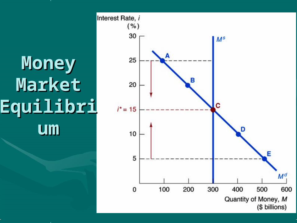
Money Money Market Market

EquilibriuEquilibriumm

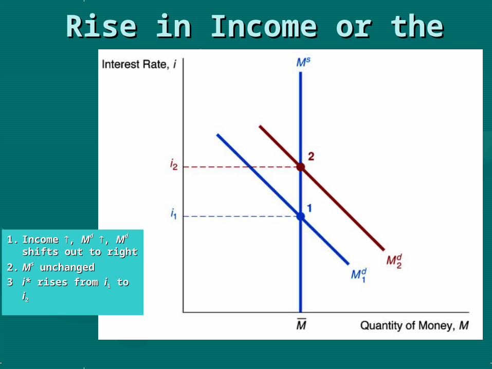
Rise in Income or the Rise in Income or the Price LevelPrice Level

1.1. Income Income , , MMdd , , MMdd shifts out to rightshifts out to right

2.2. MMss unchanged unchanged

33 ii* rises from * rises from ii11 to to ii22

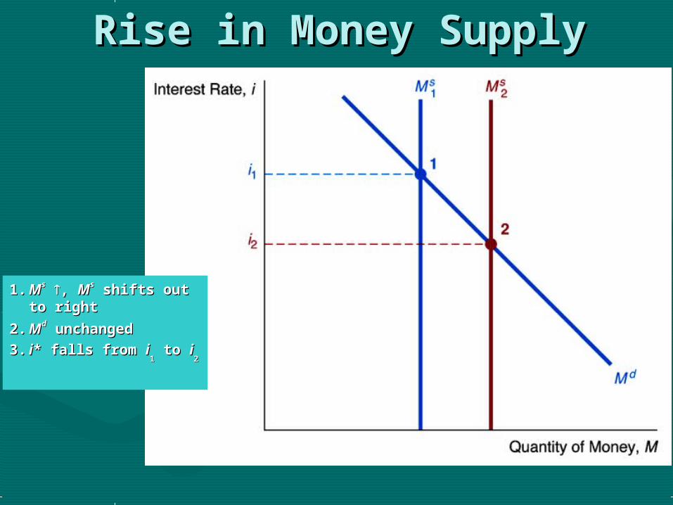
Rise in Money SupplyRise in Money Supply

1.1. MMss , , MMss shifts out shifts out to rightto right

2.2. MMdd unchanged unchanged

3.3. ii* falls from * falls from ii11 to to ii

22

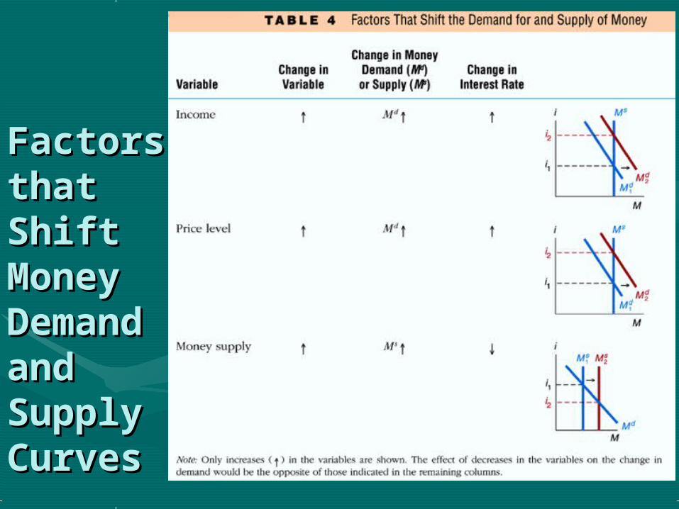
Factors Factors that that Shift Shift MoneyMoneyDemanDemand and d and Supply Supply CurvesCurves

24

LMLM Curve Curve

LM curve1. Y , Md , i Points 1, 2, 3 in figure2. Right of LM: excess Md, i to LMLeft of LM : excess Ms, i to LM

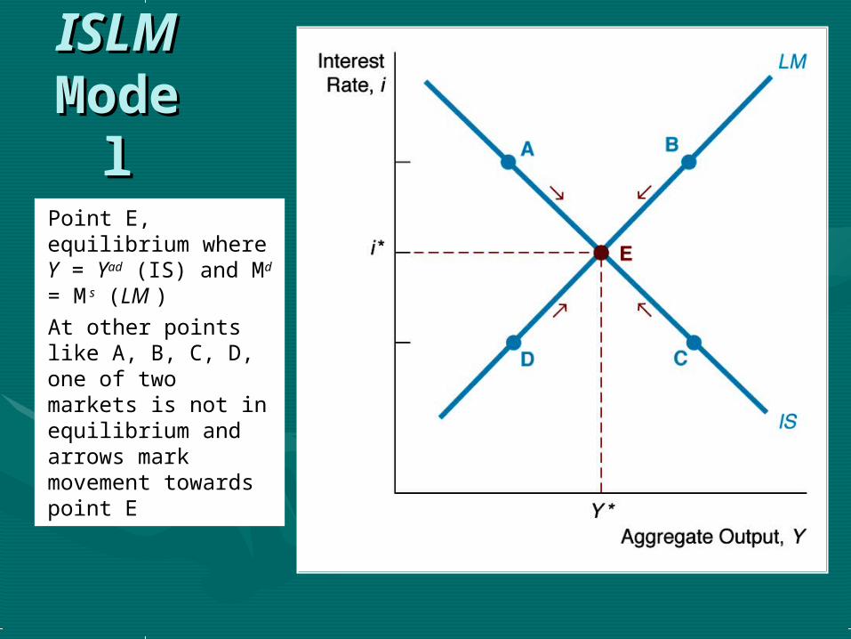
ISLISLM M

ModModelel

Point E, equilibrium where Y = Yad (IS) and Md = M s (LM )At other points like A, B, C, D, one of two markets is not in equilibrium and arrows mark movement towards point E

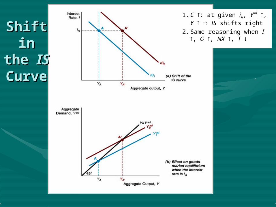
Shift Shift in the in the

ISIS CurveCurve

1. C : at given iA, Yad ,

Y IS shifts right2. Same reasoning when

I , G , NX , T

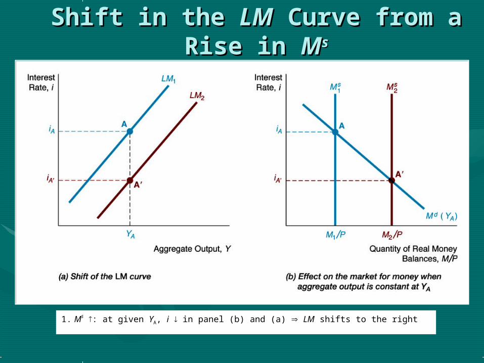
Shift in the Shift in the LMLM Curve from a Curve from a Rise in Rise in MMss

1. Ms : at given YA, i in panel (b) and (a) LM shifts to the right

Shift in the Shift in the LMLM Curve from a Curve from a Rise in Rise in MM d d

1. M d : at given YA, i in panel (b) and (a) LM shifts to the left

Response to an Increase in Response to an Increase in MMss

1. M s : i , LM shifts right Y i

Response to Expansionary Response to Expansionary Fiscal PolicyFiscal Policy

1. G or T : Yad , IS shifts right Y i

SummaSummary: ry:

Factors Factors that that

Shift Shift ISIS and and LMLM CurvesCurves

32

EffectivenEffectiveness of ess of

Monetary Monetary and Fiscal and Fiscal

PolicyPolicy

1. M d is unrelated to i i , M d = M s at same Y LM vertical

2. Panel (a): G , IS shifts right i , Y stays same (complete crowding out)

3. Panel (b): M s , Y so M d , LM shifts right i Y Conclusion: Less interest sensitive is M d, more effective is monetary policy relative to fiscal policy