7787. s87. sĒjjumsums datorzinātne un informācijas ... · sĒjjumsums datorzinātne un...
TRANSCRIPT

LATVIJAS UNIVERSITĀTES RAKSTI787. SĒJUMS787. SĒJUMS
Datorzinātne un informācijas tehnoloģijas
SCIENTIFIC PAPERS UNIVERSITY OF LATVIAVOLUME 787VOLUME 787
Computer Science and Information Technologies
LURaksti787-datorzinatne.indd 1LURaksti787-datorzinatne.indd 1 23.10.2012 12:02:1823.10.2012 12:02:18

SCIENTIFIC PAPERS UNIVERSITY OF LATVIAVOLUME 787VOLUME 787
Computer Science and Information Technologies
University of Latvia
LURaksti787-datorzinatne.indd 2LURaksti787-datorzinatne.indd 2 23.10.2012 12:02:2723.10.2012 12:02:27

Latvijas Universitāte
LATVIJAS UNIVERSITĀTES RAKSTI787. SĒJUMS787. SĒJUMS
Datorzinātne un informācijas tehnoloģijas
LURaksti787-datorzinatne.indd 3LURaksti787-datorzinatne.indd 3 23.10.2012 12:02:2723.10.2012 12:02:27

UDK 004(082) Da 814
Editorial Board
Editor-in-Chief:Prof. Jānis Bārzdiņš, University of Latvia, Latvia
Deputy Editors-in-Chief:Prof. Rūsiņš-Mārtiņš Freivalds, University of Latvia, LatviaProf. Jānis Bičevskis, University of Latvia, Latvia
Members:Prof. Andris Ambainis, University of Latvia, LatviaProf. Mikhail Auguston, Naval Postgraduate School, USAProf. Guntis Bārzdiņš, University of Latvia, LatviaProf. Juris Borzovs, University of Latvia, LatviaProf. Janis Bubenko, Royal Institute of Technology, SwedenProf. Albertas Caplinskas, Institute of Mathematics and Informatics, LithuaniaProf. Kārlis Čerāns, University of Latvia, LatviaProf. Jānis Grundspeņķis, Riga Technical University, LatviaProf. Hele-Mai Haav, Tallinn University of Technology, EstoniaProf. Kazuo Iwama, Kyoto University, JapanProf. Ahto Kalja, Tallinn University of Technology, EstoniaProf. Audris Kalniņš, University of Latvia, LatviaProf. Jaan Penjam, Tallinn University of Technology, EstoniaProf. Kārlis Podnieks, University of Latvia, LatviaProf. Māris Treimanis, University of Latvia, LatviaProf. Olegas Vasilecas, Vilnius Gediminas Technical University, Lithuania
Scientifi c secretary:Lelde Lāce, University of Latvia, Latvia
Layout: Ieva Tiltiņa
All the papers published in the present volume have been rewieved.No part on the volume may be reproduced in any form without the written permisionof the publisher.
ISSN 1407-2157 © University of Latvia, 2012ISBN 978-9984-45-569-3 © The Autors, 2012
LURaksti787-datorzinatne.indd 4LURaksti787-datorzinatne.indd 4 23.10.2012 12:02:2723.10.2012 12:02:27

Contents
Edgars Diebelis Efficiency Measurements of Self-Testing 7
Valdis Vizulis, Edgars Diebelis Self-Testing Approach and Testing Tools 27
Kaspars SudarsData Acquisition from Real World Objects based on Nonuniform Signal Sampling and Processing 50
Atis Elsts, Girts Strazdins, Andrey Vihrov, Leo Selavo Design and Implementation of MansOS: a Wireless Sensor Network Operating System 79
Sergejs Kozlovics Calculating The Layout For Dialog Windows Specified As Models 106
Madara Augstkalne, Andra Beriņa, Rūsiņš Freivalds Frequency Computable Relations 125
Nikolajs Nahimovs, Alexander Rivosh, Dmitry Kravchenko On fault-tolerance of Grover’s algorithm 136
Agnis Škuškovniks On languages not recognizable by One-way Measure Many Quantum Finite automaton 147
Jānis Iraids, Kaspars Balodis, Juris Čerņenoks, Mārtiņš Opmanis, Rihards Opmanis, Kārlis Podnieks Integer Complexity: Experimental and Analytical Results 153
LURaksti787-datorzinatne.indd 5LURaksti787-datorzinatne.indd 5 23.10.2012 12:02:2723.10.2012 12:02:27

LURaksti787-datorzinatne.indd 6LURaksti787-datorzinatne.indd 6 23.10.2012 12:02:2723.10.2012 12:02:27
Effi ciency Measurements of Self-Testing
Edgars Diebelis
University of Latvia, Raina blvd. 19, Riga, Latvia, [email protected]
This paper is devoted to efficiency measurements of self-testing, which is one of smart technology components. The efficiency measurements were based on the statistics on incidents registered for eight years in a particular software develop-ment project: Currency and Securities Accounting System. Incident notification categories have been distributed into groups in the paper: bugs that would be identified, with appropriately located test points, already in the development en-vironment, and bugs that would not be identified with the self-testing approach neither in the development, testing or production environments. The real mea-surements of the self-testing approach provided in the paper prove its efficiency and expediency.
Keywords. Testing, Smart technologies, Self-testing.
Introduction
Self-testing is one of the features of smart technologies [1]. The concept of smart technologies proposes to equip software with several built-in self-regulating mech-anisms, for examples, external environment testing [2, 3], intelligent version up-dating [4], integration of the business model in the software [5] and others. The necessity of this feature is driven by the growing complexity of information systems. The concept of smart technologies is aiming at similar goals as the concept of au-tonomous systems developed by IBM in 2001 [6, 7, 8], but is different as for the problems to be solved and the solution methods. Autonomic Computing purpose [9] is to develop information systems that are able of self-management, in this way taking down the barriers between users and the more and more complex world of information technologies. IBM outlined four key features that characterise auto-nomic computing:
• Self-configuration. Automated configuration of components and systems fol-lows high-level policies. Rest of system adjusts automatically and seamlessly.
• Self-optimization. Components and systems continually seek opportunities to improve their own performance and efficiency.
• Self-healing. System automatically detects, diagnoses, and repairs local-ized software and hardware problems.
SCIENTIFIC PAPERS, UNIVERSITY OF LATVIA, 2012. Vol. 787COMPUTER SCIENCE AND INFORMATION TECHNOLOGIES 7–26 P.
LURaksti787-datorzinatne.indd 7LURaksti787-datorzinatne.indd 7 23.10.2012 12:02:2723.10.2012 12:02:27

• Self-protection. System automatically defends against malicious attacks or cascading failures. It uses early warning to anticipate and prevent system-wide failures.
With an aim similar to an autonomic computing, the smart technologies ap-proach was offered in 2007 [1]. It provided a number of practically implementable improvements to the functionality of information systems that would make their maintenance and daily use simpler, taking us nearer to the main aim of autonomic computing. The main method offered for implementing smart technologies is not the development of autonomous universal components but the direct implementa-tion of smart technologies in particular programs.
The first results of practical implementation of smart technologies are avail-able. Intelligent version updating software is used in the Financial and budget report (FIBU) information system that manages budget planning and performance control in more than 400 government and local government organisations with more than 2000 users [4]. External environment testing [3] is used in FIBU, the Bank of Latvia and some commercial banks (VAS Hipotēku un zemes banka, AS SEB banka etc.) in Latvia. The third instance of the use of smart technologies is the integra-tion of a business model and an application [5]. The implementation is based on the concept of Model Driven Software Development (MDSD) [10], and it is used in developing and maintaining several event-oriented systems.
Self-testing provides the software with a feature to test itself automatically prior to operation. The purpose of self-testing is analogical to turning on the computer: prior to using the system, it is tested automatically that the system does not contain errors that hinder the use of the system.
The article continues to deal with the analysis of the self-testing approach. Pre-vious papers [11, 13, 14] have dealt with the ideology and implementation of the self-testing approach. As shown in [11, 12], self-testing contains two components:
• Test cases of system’s critical functionality to check functions which are substantial in using the system;
• Built-in mechanism (software component) for automated software testing (regression testing).
In order to ensure development of high quality software, it is recommendable to perform testing in three phases in different environments: development, test, production [11]. Self-testing implementation is based on the concept of Test Points [13, 14]. A test point is a programming language command in the software text, prior to execution of which testing action commands are inserted. A test point en-sures that particular actions and field values are saved when storing tests and that the software execution outcome is registered when tests are executed repeatedly. Key components of the self-testing software are: test control block for capturing and playback of tests, library of test actions, test file (XML file) [13, 14].
This paper analyses the efficiency of self-testing. Since it is practically impos-sible to test a particular system with various methods and compare them (e.g. manual
8 COMPUTER SCIENCE AND INFORMATION TECHNOLOGIES
LURaksti787-datorzinatne.indd 8LURaksti787-datorzinatne.indd 8 23.10.2012 12:02:2723.10.2012 12:02:27

Edgars Diebelis. Efficiency Measurements of Self-Testing
tests, tests using testing support tools with various features) with tests performed using the self-testing approach, another methodology for evaluating the efficiency has been used. The implementation of a comparatively large system was selected, and an expert analysed what bugs have been detected and in what stage of system development they could be detected, assuming that the self-testing functionality in the system would had been implemented from the very beginning of developing it. The analysis was based on the statistics of incident notifications registered during the system development stage, in which testing was done manually. The paper contains tables of statistics and graphs distributed by types of incident notifications, types of test points and years; this makes it possible to make an overall assessment of the efficiency of self-testing.
The paper is composed as follows: Chapter 1 briefly outlines the Currency and Securities Accounting System in order to give an insight on the system whose incident notifications were used for measuring the efficiency of the self-testing ap-proach. Chapter 2 deals in more detail with the approach used for measuring the efficiency of self-testing. Chapter 3 provides a detailed overview of the measure-ment results from various aspects, and this makes it possible to draw conclusions on the pros and cons of self-testing.
1. Currency and Securities Accounting System (CSAS)
Since the paper’s author has managed, for more than six years, the maintenance and improvement of the Currency and Securities Accounting System (CSAS), it was chosen as the test system for evaluating the self-testing approach. The CSAS, in various configuration versions, is being used by three Latvian banks:
• SEB banka (from 1996);• AS Reģionālā investīciju banka (from 2007);• VAS Latvijas Hipotēku un zemes banka (from 2008),
The CSAS is a system built in two-level architecture (client-server), and it consists of:
• client’s applications (more than 200 forms) developed in: Centura SQL Windows, MS Visual Studio C#, MS Visual Studio VB.Net;
• database management system Oracle 10g (317 tables, 50 procedures, 52 triggers, 112 functions).
The CSAS consists of two connected modules: • securities accounting module (SAM);• currency transactions accounting module (CTAM).
1.1. Securities Accounting Module (SAM)
The software’s purpose is to ensure the execution and analysis of transactions in securities. The SAM makes it possible for the bank to register customers that
9
LURaksti787-datorzinatne.indd 9LURaksti787-datorzinatne.indd 9 23.10.2012 12:02:2723.10.2012 12:02:27

hold securities accounts, securities and perform transactions in them in the name of both the bank and the customers. Apart from inputting and storing the data, the system also makes it possible to create analytical reports.
The SAM ensures the accounting of securities held by the bank and its custom-ers and transactions in them. Key functions of the SAM are:
• Inputting transaction applications. The SAM ensures the accounting of the following transactions: selling/buying securities, security transfers, trans-actions in fund units, securities transfers between correspondent accounts, deregistration of securities, repo and reverse repo transactions, encum-brances on securities, trade in options;
• Control of transaction application statuses and processing of transactions in accordance with the determined scenario;
• Information exchange with external systems. The SAM ensures information exchange with the following external systems: the bank’s internet banking facility, fund unit issuer’s system, the Latvian Central Depository, the Riga Stock Exchange, the bank’s central system, Bloomberg, SWIFT, the Asset Management System (AMS);
• Registration and processing of executed transactions;• Calculation and collection of various fees (broker, holding etc);• Revaluation of the bank’s securities portfolio, amortisation and calculation
of provisions;• Control of partner limits;• Comparing the bank’s correspondent account balances with the account
statements sent by the correspondent banks;• Making and processing money payment orders related to securities. The
SAM ensures the accounting of the following payments: payment of div-idends (also for deregistered shares), tax collection/return, coupon pay-ments, principal amount payments upon maturity;
• Making reports (inter alia to the Financial and Capital Market Commission, the Bank of Latvia, securities account statements to customers).
The SAM ensures swift recalculation of securities account balances based on transactions. The SAM is provided with an adjustable workplace configuration.
1.2. Currency Transactions Accounting Module (CTAM)
The purpose of the software is to account and analyse currency transactions (currency exchange, interbank deposits etc). The system accounts currency trans-actions and customers who perform currency transactions. Apart from data ac-counting, the system provides its users with analytical information on customers, currency transactions and currency exchange rates.
10 COMPUTER SCIENCE AND INFORMATION TECHNOLOGIES
LURaksti787-datorzinatne.indd 10LURaksti787-datorzinatne.indd 10 23.10.2012 12:02:2723.10.2012 12:02:27
Edgars Diebelis. Efficiency Measurements of Self-Testing
Key functions of the CTAM are:• Inputting transactions. The CTAM ensures the accounting of the following
transactions: interbank FX, FX Forward, SWAP (risk, risk-free), interbank depositing, (in/out/extension); customer FX, FX Forward, SWAP (risk, risk-free), interbank depositing, (in/out/extension), floating rate, interbank order, customer order, interest rate swaps, options, State Treasury transac-tions, collateral transactions, currency swap transactions;
• Control of transaction status and processing of transactions in accordance with the determined scenario (workflow);
• Information exchange with external systems. The CTAM ensures informa-tion exchange with the following external systems: bank’s central system, Reuter, UBS TS trading platform, SWIFT;
• Maintaining currency positions (bank’s total position, positions per port-folios);
• Setting and controlling limits;• Importing transactions from Reuter and Internet trading platforms (TS,
UBS TS etc);• Importing currency exchange rates and interest rates from Reuters;• Margin trading;• Nostro account balances;• Making reports.
The CTAM is provided with an adjustable workplace configuration.
2. Self-testing Effi ciency Measurements Approach
All incident notifications (1,171 in total) in the CSAS in the period from July 2003 to 23 August 2011 retrieved from the Bugzilla [15] incident logging sys-tem were analysed. Since the incident logging system is integrated with a work time accounting system, in the efficiency measurements not only the quantity of incidents registered but also the time consumed to resolve incidents was used. Every incident notification was evaluated using the criteria provided in Table 1. As it can be seen in the table, not all incident notifications have been classified as bugs. Users register in the incident logging system also incidents that, after investigating the bug, in some cases get reclassified as user errors, improvements or consultations.
11
LURaksti787-datorzinatne.indd 11LURaksti787-datorzinatne.indd 11 23.10.2012 12:02:2723.10.2012 12:02:27

Table 1Types of Incident Notifi cations
Type of Incident DescriptionUnidentifiable bug Incident notifications that described an actual bug in the
system and that would not be identified by the self-testing approach if the system had a self-testing approach tool implemented.
Identifiable bug Incident notifications that described an actual bug in the system and that would be identified by the self-testing approach if the system had a self-testing approach tool implemented.
Duplicate Incident notifications that repeated an open incident notification
User error Incident notifications about which, during resolving, it was established that the situation described had occurred due to the user’s actions.
Improvement Incident notifications that turned out to be system functionality improvements.
Consultation Incident notifications that were resolved by way of consultations.
For measuring the efficiency of the self-testing approach, the most important types of incident notifications are Identifiable Bug and Unidentifiable Bug. Therefore, these types of incident notifications are looked at in more detail on the basis of the distribution of incidents by types provided in the tables below (Table 2 and Table 3).
Table 2Unidentifi able Bug; Distribution of Notifi cations by Bug Types
Bug type DescriptionExternal interface bug Error in data exchange with the external systemComputer configuration bug
Incompliance of user computer’s configuration with the requirements of the CSAS.
Data type bug Inconsistent, incorrect data type used. Mismatch between form fields and data base table fields
User interface bug Visual changes. For example, a field is inactive in the form or a logo is not displayed in the report.
Simultaneous users actions bug
Simultaneous actions by multiple users with one record in the system.
Requirement interpretation bug
Incomplete customer’s requirements. Erroneous interpretation of requirements by the developer.
Specific event Specific uses of the system resulting in a system error.
12 COMPUTER SCIENCE AND INFORMATION TECHNOLOGIES
LURaksti787-datorzinatne.indd 12LURaksti787-datorzinatne.indd 12 23.10.2012 12:02:2723.10.2012 12:02:27

Edgars Diebelis. Efficiency Measurements of Self-Testing
Table 3Identifi able Bug; Distribution of Notifi cations by Test Point Types
Test point that would identify the bug
Description
File result test point The test point provides the registration of the values to be read from and written to the file, inter alia creation of the file.
Input field test point This test point registers an event of filling in a field.Application event test point This test point would register any events performed in the
application, e.g. clicking on the Save button;Comparable value test point
This test point registers the values calculated in the system. The test point can be used when the application contains a field whose value is calculated considering the values of other fields, the values of which are not saved in the database.
System message test point This test point is required to be able to simulate the message box action, not actually calling the messages.
SQL query result test point This test point registers specific values that can be selected with an SQL query and that are compared in the test execution mode with the values selected in test storing and registered in the test file.
3. Results of Measurements
3.1. Distribution of Notifi cations by Incident Types and Time Consumed
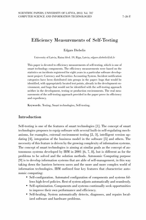
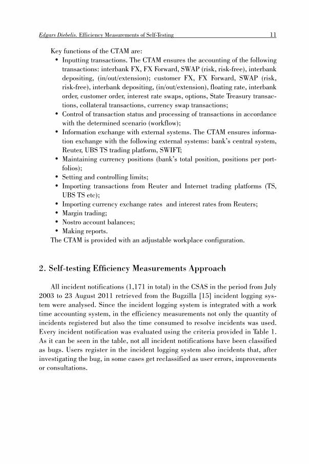
Table 4 shows a distribution of all incident notifications by incident types and the time consumed to resolve them in hours. The table contains the following col-umns:
• Notification type – incident notification type (Table 1);• Quantity – quantity of incident notifications• % of total – percentage of a particular notification type in the total quantity
of incident notifications;• Hours – total time consumed to resolve one type of incident notifications;• % of total – percentage of the time spent to resolve the particular notifica-
tion type of the total time spent for resolving all incident notifications.
13
LURaksti787-datorzinatne.indd 13LURaksti787-datorzinatne.indd 13 23.10.2012 12:02:2723.10.2012 12:02:27
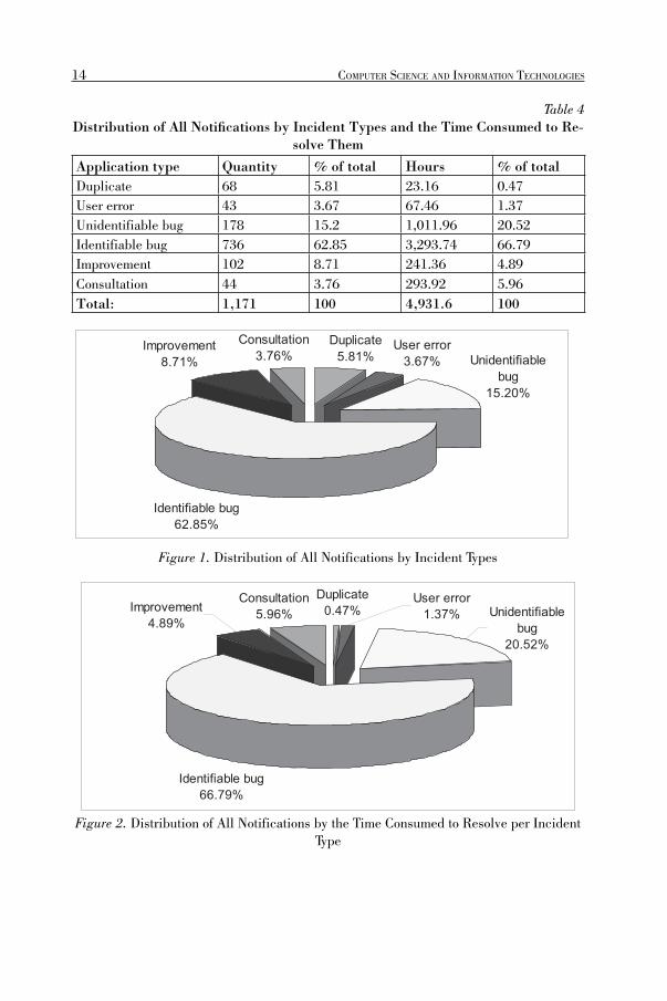
Table 4Distribution of All Notifi cations by Incident Types and the Time Consumed to Re-
solve Them
Application type Quantity % of total Hours % of totalDuplicate 68 5.81 23.16 0.47User error 43 3.67 67.46 1.37Unidentifiable bug 178 15.2 1,011.96 20.52Identifiable bug 736 62.85 3,293.74 66.79Improvement 102 8.71 241.36 4.89Consultation 44 3.76 293.92 5.96Total: 1,171 100 4,931.6 100
Duplicate5.81%
User error3.67% Unidentifiable
bug15.20%
Identifiable bug62.85%
Improvement8.71%
Consultation3.76%
F igure 1. Distribution of All Notifications by Incident Types
Identifiable bug66.79%
Consultation5.96%Improvement
4.89%Unidentifiable
bug20.52%
User error1.37%
Duplicate0.47%
Figure 2. Distribution of All Notifications by the Time Consumed to Resolve per Incident Type
14 COMPUTER SCIENCE AND INFORMATION TECHNOLOGIES
LURaksti787-datorzinatne.indd 14LURaksti787-datorzinatne.indd 14 23.10.2012 12:02:2723.10.2012 12:02:27

Edgars Diebelis. Efficiency Measurements of Self-Testing
Considering the information obtained, the author concludes that:• Of the total quantity of incident notifications (1,171), if the self-testing
approach had been implemented in the CSAS, 62.85% (736 notifications, 3,293.74 hours consumed for resolving) of all the incident notifications registered in nearly nine years would had been identified by it already in the development stage. It means that developers would had been able to identify and repair the bugs already in the development stage, which would significantly improve the system’s quality and increase the customer’s trust about the system’s quality. Measurements similar to [16] show the advan-tages of systematic testing compared to manual.
• As mentioned in many sources [17], the sooner a bug is identified, the lower the costs of repairing it. The differences mentioned reach to ten and even hundred times. The time spent for repairing bugs as provided in Table 4 would be definitely lower if the bugs had been identified already in the development stage. Assuming that the identification of bugs in the devel-opment stage would allow saving 50% of the time consumed for repairing all the bugs identified by the customer, about 1,650 hrs, or about 206 work-ing days, could have been saved in the period of nine years.
• Of the total quantity of incident notifications, the self-testing approach in the CSAS would not be able to identify 15.2% of the bugs (178 notifica-tions, 1,011.74 hours consumed for repairing) of the total number of inci-dent notifications.
• Of the total quantity of incident notifications, 78.05% (914 notifications, 4,305.7 hours consumed for repairing) were actual bugs that were repaired, other 11.95% (257 notifications, time consumed for repairing 625.9 hours) of incident notifications were user errors, improvements, consultations and bug duplicates that cannot not be identified with testing.
• The time consumed for repairing bugs in percentage (87.31%) of the to-tal time consumed for incident notifications is higher than the percentage (78.05%) of bugs in the total quantity of incident notifications. This means that more time has been spent to repair bugs proportionally to other inci-dent notifications (improvements, user errors, consultations to users and bug duplicates).
3.2. Distribution of Notifi cations by Bug Types
As mentioned in the previous Chapter, there are two types of incident notifica-tions that are classified as bugs: Unidentifiable Bugs and Identifiable Bugs, and they are analysed in the next table (Table 5). The table columns’ descriptions are the same as in the previous Chapter.
15
LURaksti787-datorzinatne.indd 15LURaksti787-datorzinatne.indd 15 23.10.2012 12:02:2723.10.2012 12:02:27

Table 5 Distribution of Bugs by Bug Types
Bug Type Quantity % of total Hours % of totalUnidentifiable bug 178 19.47 1011.96 23.5Identifiable bug 736 80.53 3293.74 76.5Total: 914 100 4305.7 100
Identifiable bug; 80.53
Unidentifiable bug; 19.47
Figure 3. Distribution of Bugs by Bug Types
Unidentifiable bug; 23.5
Identifiable bug; 76.5
Figure 4. Distribution of Bugs by Bug Types per Time Consumed
Considering the information obtained, the author concludes that:• The self-testing approach would identify 80% of all the bugs registered in
the CSAS.• The time consumed for repairing the bugs identified by the self-testing
approach in percent (76.5%) of the total time consumed for resolving is lower than the percentage (80.53%) of these bugs in the total quantity of bugs. This means that less time would be spent to repair the bugs identified with the self-testing approach proportionally to the bugs that would not be identified with self-testing.
16 COMPUTER SCIENCE AND INFORMATION TECHNOLOGIES
LURaksti787-datorzinatne.indd 16LURaksti787-datorzinatne.indd 16 23.10.2012 12:02:2723.10.2012 12:02:27

Edgars Diebelis. Efficiency Measurements of Self-Testing
3.3. Distribution of Notifi cations by Years
T he next table (Table 6) shows the distribution of incident notifications by years. The table contains the following columns:
• Notification type - quantity of incident notifications by type (Table 1) per years; - % of total – percentage of a particular notification type in the total
quantity of incident notifications per year;• 2003-2011 – years analysed;
Table 6Distribution of Notifi cations by Years
Notifi cation type 2003 2004 2005 2006 2007 2008 2009 2010 2011Duplicate 1 1 13 22 7 10 7 5 2% of total 3.23 1.3 13.13 10.19 4.9 5.29 3.45 3.85 2.41User error 2 6 3 10 1 7 5 3 6% of total 6.45 7.79 3.03 4.63 0.7 3.7 2.46 2.31 7.23Unidentifiable bug 2 7 11 19 19 37 38 23 22% of total 6.45 9.09 11.11 8.8 13.29 19.58 18.72 17.69 26.51Identifiable bug 17 51 59 138 98 110 141 79 43% of total 54.84 66.23 59.6 63.89 68.53 58.2 69.46 60.77 51.81Improvement 9 12 13 25 11 11 6 11 4% of total 29.03 15.58 13.13 11.57 7.69 5.82 2.96 8.46 4.82Consultation 0 0 0 2 7 14 6 9 6% of total 0 0 0 0.93 4.9 7.41 2.96 6.92 7.23Total: 31 77 99 216 143 189 203 130 83
From the table it can be seen that:• In some years, there are peaks and falls in the number of some incident
notification types; also, consultation-type incident notifications have been registered as from 2005, but their proportional distribution by years match approximately the total proportional distribution of notifications.
• In any of the year’s most of the bugs notified could be identified with the self-testing approach.
3.4. Distribution of Bugs by Years
The next table (Table 7) shows the distribution of bugs separately. The table contains the following columns:
• Year – years (2003-2011) analysed;
17
LURaksti787-datorzinatne.indd 17LURaksti787-datorzinatne.indd 17 23.10.2012 12:02:2823.10.2012 12:02:28
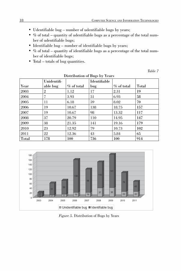
• Udentifiable bug – number of udentifiable bugs by years;• % of total – quantity of udentifiable bugs as a percentage of the total num-
ber of udentifiable bugs;• Identifiable bug – number of identifiable bugs by years;• % of total – quantity of identifiable bugs as a percentage of the total num-
ber of identifiable bugs;• Total – totals of bug quantities.
Table 7Distribution of Bugs by Years
YearUnidentifi -able bug % of total
Identifi able bug % of total Total
2003 2 1.12 17 2.31 192004 7 3.93 51 6.93 582005 11 6.18 59 8.02 702006 19 10.67 138 18.75 1572007 19 10.67 98 13.32 1172008 37 20.79 110 14.95 1472009 38 21.35 141 19.16 1792010 23 12.92 79 10.73 1022011 22 12.36 43 5.84 65Total 178 100 736 100 914
217
7
51
11
59
19
138
19
98
37
110
38
141
23
79
22
43
0
20
40
60
80
100
120
140
160
180
2003 2004 2005 2006 2007 2008 2009 2010 2011
Unidentifiable bug Identifiable bug
Figure 5. Distribution of Bugs by Years
18 COMPUTER SCIENCE AND INFORMATION TECHNOLOGIES
LURaksti787-datorzinatne.indd 18LURaksti787-datorzinatne.indd 18 23.10.2012 12:02:2823.10.2012 12:02:28

Edgars Diebelis. Efficiency Measurements of Self-Testing
1.12
3.93
6.18
10.67 10.67
20.79 21.35
12.92 12.36
2.31
6.938.02
18.75
13.3214.95
19.16
10.73
5.84
0
5
10
15
20
25
2003 2004 2005 2006 2007 2008 2009 2010 2011
Unidentifiable bug Identifiable bug
Figure 6. Distribution of Bugs in Percent by Years
Considering the information obtained, the author concludes that:• The self-testing approach would identify most of the bugs registered in the
CSAS.• Changes, by years, in the percentages of the bugs identified and not identi-
fied with the self-testing approach are not significant. • In the first five years, the weighting of the bugs that could be identified
with the self-testing approach is higher, but later the weighting of the bugs that could not be identified with the self-testing approach becomes higher. This shows that the “simpler” bugs are discovered sooner than the “non-standard” ones.
3.5. Ratio of the Bug Volume to the Improvement Expenses Distributed by Years
The next table (Table 9) shows the ratio of the quantity of bugs to the volume of improvement expenses by years. The table contains the following columns:
• Year – years analysed;• Quantity of bugs – quantity of bugs registered in the CSAS by years;• % of total – distribution of the quantity of bugs in percent by years;• Improvement expenses in % of total – percentage of the amount spent for
improvements by years;
19
LURaksti787-datorzinatne.indd 19LURaksti787-datorzinatne.indd 19 23.10.2012 12:02:2823.10.2012 12:02:28

Table 8Ratio of the Bug Quantity to the Improvement Expenses Distributed by Years
YearQuantity of bugs % to total
Improvement expenses in % of total
2003 31 2.65 2.862004 77 6.58 12.382005 99 8.45 15.252006 216 18.45 15.132007 143 12.21 11.042008 189 16.14 21.622009 203 17.34 9.772010 130 11.1 6.242011 83 7.09 5.71Total: 1,171 100 100
2.65
6.588.45
18.45
12.21
16.1417.34
11.1
7.09
2.86
12.38
15.25 15.13
11.04
21.62
9.77
6.24 5.71
0
5
10
15
20
25
2003 2004 2005 2006 2007 2008 2009 2010 2011
Quantity of Notifications Improvement Expenses
Figure 7. Ratio of the Quantity of Notifications to the Improvement Expenses
The information looked at in this Sub-chapter does not directly reflect the ef-ficiency of the self-testing approach, but it is interesting to compare changes in the quantity of notifications (%) and in the improvement expenses (%) during the nine years. Considering the information obtained, it can be concluded that, as the improvement volumes grow, also the bug volumes grow. The conclusion is a rather logical one, but in this case it is based on an actual example.
20 COMPUTER SCIENCE AND INFORMATION TECHNOLOGIES
LURaksti787-datorzinatne.indd 20LURaksti787-datorzinatne.indd 20 23.10.2012 12:02:2823.10.2012 12:02:28

Edgars Diebelis. Efficiency Measurements of Self-Testing
3.6. Distribution of the Bugs Unidentifi able by the Self-Testing Approach by Types
The next table (Table 9) shows the distribution of bugs unidentifiable by the self-testing approach by bug types. The table contains the following columns:
• Bug type – one of seven bug types;• Quantity – quantity of bugs of the type;• % of total – percentage of the bug type in the total quantity of bugs.
Table 9Distribution of the Bugs Unidentifi able by the Self-Testing Approach by Types
Bug type Quantity % of TotalExternal interface bug 5 2.81Computer configuration bug 12 6.74Data type bug 7 3.93User interface bug 25 14.04Simultaneous actions by users 5 2.81Requirement interpretation bug 41 23.03Specific event 83 46.63Total: 178 100
Specific event46.63%
Requirement interpretation bug
23.03%
Simultaneous actions by users
2.81%
User interface bug14.04%
Data type bug3.93%
Computer configuration bug
6.74%
External interface bug
2.81%
Figure 8. Distribution of the Bugs Unidentifiable by the Self-Testing Approach by Types
Conclusions:• Most (nearly 50%) of the bugs that the self-testing approach would not
be able to identify are specific cases that had not been considered when developing the system. For example, the following scenario from a bug de-scription: “I enter the login, password, press Enter, press Enter once again, then I press Start Work, in the tree I select any view that has items under it. And I get an error!”. As it can be seen, it is a specific case that the
21
LURaksti787-datorzinatne.indd 21LURaksti787-datorzinatne.indd 21 23.10.2012 12:02:2823.10.2012 12:02:28

developer had not considered. To test critical functionality, a test example that plans that Enter is pressed once would be made, and this test example would not result in a bug. Furthermore, a scenario that plans that Enter is pressed twice would not be created since it is a specific case not performed by users in their daily work. The self-testing approach is not able to iden-tify bugs that occur due to various external devices. For example, when a transaction confirmation is printed, the self-testing approach would not be able to detect that one excessive empty page will be printed with it.
• One fifth of the total quantity of the bugs that the self-testing approach would be unable to identify are requirement interpretation bugs. Bugs of this type occur when system additions/improvements are developed and the result does not comply with the customer’s requirements because the developer had interpreted the customer’s requirements differently. To the author’s mind, the quantity of hours (41) during the nine-year period is small and is permissible.
• The self-testing approach is unable to identify visual changes in user inter-faces, data formats, field accessibility and similar bugs.
• A part of the registered bugs are related to incompliance of the user com-puter’s configuration with the system requirements. The self-testing ap-proach would be able to identify bugs of this type only on the user com-puter, not on the testing computer that has been configured in compliance with the system requirements.
• A part of the bugs that the self-testing approach would be unable to identify are data type bugs that include:
- checking that the window field length and data base table field length match;
- exceeding the maximum value of the variable data type.• The self-testing approach is unable to identify bugs that result from the
data of external interfaces with other systems. The self-testing approach is able to store and execute test examples that contain data from external interfaces, but it is unable to create test examples that are not compliant with the requirements of the external system (e.g. a string of characters in-stead of digits is given by the internal interface). Of course, it is possible to implement a control in the system itself that checks that the data received from the external interface are correct.
• The self-testing approach is unable to identify bugs that result from trans-action mechanisms incorrectly implemented in the system, e.g. if several users can simultaneously modify one and the same data base record.
22 COMPUTER SCIENCE AND INFORMATION TECHNOLOGIES
LURaksti787-datorzinatne.indd 22LURaksti787-datorzinatne.indd 22 23.10.2012 12:02:2823.10.2012 12:02:28

Edgars Diebelis. Efficiency Measurements of Self-Testing
3.7. Distribution of the Bugs Identifi able by the Self-Testing Approach by Test Point Types
The next table (Table 10) shows the distribution of bugs identifiable by the self-testing approach by bug types and time consumed to resolve them. The table contains the following columns:
• Test point – test point that would identify the bug;• Quantity – quantity of bugs that the test point would identify;• % of total – percentage of the bugs that would be repaired by the test point
in the total quantity of bugs that would be repaired by all test points;• Hours – hours spent to resolve the bugs that the test points could identify;• % of total – percentage of hours in the total number of hours consumed to
repair the bugs that could be identified by test points.
Table 10Distribution of the Bugs Identifi able
by the Self-Testing Approach by Test Point Types Test point Quantity % of total Hours % of totalFile result test point 59 8.02 150.03 4.56Entry field test point 146 19.84 827.14 25.11Application event test point 105 14.27 364.24 11.06Comparable value test point 28 3.8 93.53 2.84System message test point 11 1.49 58.84 1.79SQL query result test point 387 52.58 1,799.96 54.65Total: 736 100 3,293.74 100
File result test point; 8.02SQL query result
test point; 52.58
Entry field test point; 19.84
Application event test point; 14.27
Comparable value test point; 3.8
System message test point; 1.49
Figure 9. Distribution of the Bugs Identifiable by the Self-Testing Approach by Test Point Types
23
LURaksti787-datorzinatne.indd 23LURaksti787-datorzinatne.indd 23 23.10.2012 12:02:2823.10.2012 12:02:28

Conclusions:• More than a half of all the registered bugs could be identified with the SQL
query result test point. At the test point, data are selected from the data base and compared with the benchmark values. The explanation is that the key purpose of the CSAS is data storing and making reports using the stored data.
• One fifth of the bugs that could be identified with the self-testing approach would be identified by the input field test point. The test point compares the field value with the benchmark value.
4. Conclusions
In order to present advantages of self-testing, the self-testing features are in-tegrated in the CSAS, a large and complex financial system. Although efforts are ongoing, the following conclusions can be drawn from the CSAS experience:
• Using the self-testing approach, developers would have been able to iden-tify and repair 80% of the bugs already in the development stage; accord-ingly, 63% of all the received incident notifications would have never oc-curred. This would significantly improve the system’s quality and increase the customer’s trust about the system’s quality.
• A general truth is: the faster a bug is identified, the lower the costs of repairing it. The self-testing approach makes it possible to identify many bugs already in the development stage, and consequently the costs of re-pairing the bugs could be reduced, possibly, by two times.
• Most of the bugs that the self-testing approach would be unable to identify are specific cases of system use.
• The SQL query result test point has a significant role in the identification of bugs; in the system analysed herein, it would had identified more than a half of the bugs notified.
From the analysis of the statistics, it can be clearly concluded that the im-plementation of self-testing would make it possible to save time and improve the system quality significantly. Also, the analysis has shown that the self-testing ap-proach is not able to identify all system errors. On the basis of the analysis provided herein, further work in evolving the self-testing approach will be aimed at reducing the scope of the types of bugs that the current self-testing approach is unable to identify.
24 COMPUTER SCIENCE AND INFORMATION TECHNOLOGIES
LURaksti787-datorzinatne.indd 24LURaksti787-datorzinatne.indd 24 23.10.2012 12:02:2823.10.2012 12:02:28
Edgars Diebelis. Efficiency Measurements of Self-Testing
IEGULDĪJUMS TAVĀ NĀKOTNĒ
This work has been supported by the European Social Fund within the project «Support for Doctoral Studies at University of Latvia».
References
1. Bičevska, Z., Bičevskis, J.: Smart Technologies in Software Life Cycle. In: Münch, J., Abraha-msson, P. (eds.) Product-Focused Software Process Improvement. 8th International Conference, PROFES 2007, Riga, Latvia, July 2-4, 2007, LNCS, vol. 4589, pp. 262-272. Springer-Verlag, Berlin Heidelberg (2007).
2. Rauhvargers, K., Bicevskis, J.: Environment Testing Enabled Software - a Step Towards Execution Context Awareness. In: Hele-Mai Haav, Ahto Kalja (eds.) Databases and Information Systems, Selected Papers from the 8th International Baltic Conference, IOS Press vol. 187, pp. 169-179 (2009).
3. Rauhvargers, K.: On the Implementation of a Meta-data Driven Self Testing Model. In: Hruška, T., Madeyski, L., Ochodek, M. (eds.) Software Engineering Techniques in Progress, Brno, Czech Republic (2008).
4. Bičevska, Z., Bičevskis, J.: Applying of smart technologies in software development: Automated version updating. In: Scientific Papers University of Latvia, Computer Science and Information Technologies, vol .733, ISSN 1407-2157, pp. 24-37 (2008).
5. Ceriņa-Bērziņa J.,Bičevskis J., Karnītis Ģ.: Information systems development based on visual Domain Specific Language BiLingva. In: Preprint of the Proceedings of the 4th IFIP TC 2 Cen-tral and East Europe Conference on Software Engineering Techniques, CEE-SET 2009, Krakow, Poland, Oktober 12-14, 2009, pp. 128-137.
6. Ganek, A. G., Corbi, T. A.: The dawning of the autonomic computing era. In: IBM Systems Jour-nal, vol. 42, no. 1, pp. 5-18 (2003).
7. Sterritt, R., Bustard, D.: Towards an autonomic computing environment. In: 14th International Workshop on Database and Expert Systems Applications (DEXA 2003), 2003. Proceedings, pp. 694 - 698 (2003).
8. Lightstone, S.: Foundations of Autonomic Computing Development. In: Proceedings of the Fourth IEEE international Workshop on Engineering of Autonomic and Autonomous Systems, pp. 163-171 (2007).
9. Kephart, J., O., Chess, D., M. The Vision of Autonomic Computing. In: Computer Magazine, vol. 36, pp.41-50 (2003).
10. Barzdins, J., Zarins, A., Cerans, K., Grasmanis, M., Kalnins, A., Rencis, E., Lace, L., Liepins, R., Sprogis, A., Zarins, A.: Domain Specific languages for Business Process Managment: a Case Study Proceedings of DSM’09 Workshop of OOPSLA 2009, Orlando, USA.
11. Diebelis, E., Takeris, V., Bičevskis, J.: Self-testing - new approach to software quality assurance. In: Proceedings of the 13th East-European Conference on Advances in Databases and Informa-tion Systems (ADBIS 2009), pp. 62-77. Riga, Latvia, September 7-10, 2009.
12. Bičevska, Z., Bičevskis, J.: Applying Self-Testing: Advantages and Limitations. In: Hele-Mai Haav, Ahto Kalja (eds.) Databases and Information Systems, Selected Papers from the 8th Inter-national Baltic Conference, IOS Press vol. 187, pp. 192-202 (2009).
25
LURaksti787-datorzinatne.indd 25LURaksti787-datorzinatne.indd 25 23.10.2012 12:02:2823.10.2012 12:02:28

13. Diebelis, E., Bičevskis, J.: An Implementation of Self-Testing. In: Proceedings of the 9th In-ternational Baltic Conference on Databases and Information Systems (Baltic DB&IS 2010), pp. 487-502. Riga, Latvia, July 5-7, 2010.
14. Diebelis, E., Bicevskis, J.: Test Points in Self-Testing. In: Marite Kirikova, Janis Barzdins (eds.) Databases and Information Systems VI, Selected Papers from the Ninth International Baltic Con-ference. IOS Press vol. 224, pp. 309-321 (2011).
15. Bugzilla [Online] [Quoted: 20.05.2012] http://www.bugzilla.org/16. Bičevskis, J.: The Effictiveness of Testing Models. In: Proc. of 3d Intern. Baltic Workshop “Data-
bases and Information Systems”, Riga, 1998.17. Pressman, R.S., Ph.D., Software Engineering, A Practitioner’s Approach. 6th edition, 2004.
26 COMPUTER SCIENCE AND INFORMATION TECHNOLOGIES
LURaksti787-datorzinatne.indd 26LURaksti787-datorzinatne.indd 26 23.10.2012 12:02:2923.10.2012 12:02:29

Self-Testing Approach and Testing Tools
Valdis Vizulis, Edgars Diebelis
Datorikas Institūts DIVI, A. Kalniņa str. 2-7, Rīga, Latvia, [email protected]
The paper continues to analyse the self-testing approach by comparing features of the self-testing tool developed with those of seven globally acknowledged testing tools. The analysis showed that the features offered by the self-testing tool are equal to those provided by other globally acknowledged testing support tools, and outperform them in instances like testing in the production environ-ment, testing of databases and cooperation in testing with external systems. Fur-thermore, the self-testing approach makes it possible for users with minimal IT knowledge to perform testing.
Keywords. Testing, Smart technologies, Self-testing, Testing tools.
Introduction
Already since the middle of the 20th century, when the first programs for comput-ers were written, their authors have been stumbling on errors. Finding errors in programs was rather seen as debugging, not testing. Only starting from 1980s, finding errors in a program in order to make sure that the program is of good quality became the main goal of testing. [1]
Since then, software requirements and their complexity accordingly have grown constantly. Along the way, various testing methods, strategies and approaches have been developed. If years ago testing was done mainly manually, in our days, as system volumes and complexity grow, various automated solutions that are able to perform the process as fast as possible and consuming as possibly little resources are sought after.
One of ways of saving both time and resources consumed, improving the quality of the system at the same time, is the system self-testing approach [2]. This ap-proach is one of smart technologies, and it enables the system to verify itself that the software is working correctly. Smart technology is based on the idea of software that is able to “manage itself” by ensuring a control over internal and external factors of the software and reacting to them accordingly. The concept of smart technologies besides a number of significant features also includes external environment testing [3, 4], intelligent version updating [5], integration of the business model in the soft-
SCIENTIFIC PAPERS, UNIVERSITY OF LATVIA, 2012. Vol. 787COMPUTER SCIENCE AND INFORMATION TECHNOLOGIES 27–49 P.
LURaksti787-datorzinatne.indd 27LURaksti787-datorzinatne.indd 27 23.10.2012 12:02:2923.10.2012 12:02:29

ware [6]. The concept of smart technologies is aiming at similar goals as the concept of autonomous systems developed by IBM in 2001 [7, 8, 9].
The key feature of self-testing is the possibility to integrate the testing support option in the system to be tested, in this way ensuring automated testing at any time and in any of the following environments: development, testing and production. To demonstrate the usefulness of the self-testing approach, a self-testing tool that can be compared with globally popular testing tools has been developed. Therefore, the main goal of this paper was, by studying and comparing the concepts, builds and features of various globally recognized testing tools, to evaluate the usefulness of the self-testing approach and tool, directions for further development and opportu-nities in the area of testing.
As shown in [10, 11], self-testing contains two components:• Test cases of system’s critical functionality to check functions which are
substantial in using the system;• Built-in mechanism (software component) for automated software testing
(regression testing) that provides automated storing and playback of tests (executing of test cases and comparing the test results with the standard values).
The defining of critical functionality and preparing tests, as a rule, is a part of requirement analysis and testing process. The self-testing software is partly in-tegrated in the testable system [12, 13], which has several operating modes; one of them is self-testing mode when an automated execution of test cases (process of testing) is available to the user. After testing, the user gets a testing report that includes the total number of tests executed, tests executed successfully, tests failed and a detailed failure description. The options provided by self-testing software are similar to the functionality of testing support tools. Unlike them, the self-testing software is part of the system to be developed. It means that there is no need to install additional testing tools for system testing at the system developers, custom-ers or users.
The paper is composed as follows: Chapter 1 describes the principles used to select the testing tools to be compared with the self-testing approach. Also, the selected testing tools are described in brief in this Chapter. Chapter 2 provides a description of the criteria used to compare the self-testing approach and the testing tools and a comparison of them.
1. Testing Tools
1.1. Selecting the testing tools
Nowadays a wide range of testing tools is available, and they are intended for various testing levels on different systems. When developing one’s own testing tool,
28 COMPUTER SCIENCE AND INFORMATION TECHNOLOGIES
LURaksti787-datorzinatne.indd 28LURaksti787-datorzinatne.indd 28 23.10.2012 12:02:2923.10.2012 12:02:29
Valdis Vizulis, Edgars Diebelis. Self-Testing Approach and Testing Tools
it is important to find out what testing tools are being offered by other developers and what are their advantages and disadvantages.
Considering that the self-testing tool employs, in a direct way, the principles of automated testing, various automated testing tools were selected for comparing. In selecting the tools to be compared, the opinion of the Automated Testing Institute (ATI), which is a leading authority in the field of testing, was used. Since May 2009, the ATI has been publishing its magazine Automate Software Testing [14], which is one of the most popular in the field of testing and has its own website too [15]. The website offers articles by experienced IT professionals on the automated testing approach, frameworks and tools; the website has a list of 716 automated testing tools available in the world and brief descriptions of them. Also, a closed forum is active; its users are registered only after approval (currently there are about 8,000 users registered).
The ATI organises an annual conference on automated testing, called Verify/ATI [16], during which new approaches and tools are demonstrated and training on them is provided. Since 2009, the company has been nominating the leading au-tomated testing tools in various categories awarding them with the ATI Automation Honors [17]. Winners of the award are selected by a committee that is composed of IT professionals, and they study the tools (information on tools is obtained from their official websites, documentation, various articles, blogs, forums etc) and nar-row down the list of tools applied for the award to five finalists in each category and sub-category (categories in 2010 ) [18]:
• Best open source code automated unit testing tool; sub-categories: C++, Java, .NET.
• Best open source code automated functional testing tool; sub-categories: WEB, Java, .NET, Flash/Flex.
• Best open source code automated performance testing tool; sub-categories: WEB, WEB services/SOA.
• Best commercial automated functional testing tool; sub-categories: WEB, Java, .NET, Flash/Flex, WEB services/SOA.
• Best commercial automated performance testing tool; sub-categories: WEB/HTTPS, WEB services/SOA.
For the comparison of the self-testing approach and testing tools in this paper, tools that have won an award in one of the aforementioned nominations were used. In the following sub-chapters of this paper, some of the award winners that are most similar to the self testing approach have been described in brief.
1.2. TestComplete
TestComplete is an automated self-testing tool developed by SmartBear; it pro-vides the testing of Windows and web applications and is one of the leading func-tional testing tools in the world. This is also proven by the fact that the tool has won the ATI Automation Honors award as the Best Commercial Automated Functional Testing Tool in 2010, and it is used in their projects by world’s leading companies like Adobe, Corel, Falafel Software, ARUP Laboratories, QlikTech etc. [19]
29
LURaksti787-datorzinatne.indd 29LURaksti787-datorzinatne.indd 29 23.10.2012 12:02:2923.10.2012 12:02:29

Concept
The TestComplete tool uses a keyword-driven testing framework to perform functional tests; in addition, with it it is possible to also develop tests with scripts. Its operation concept is comparatively simple. As shown in Figure 1, the tool, through inter-process communication and various built-in auxiliary tools, records the actions performed in the tested system and after that also executes them.
Inter-process communica�on
Tested system Test report
Figu re 1. TestComplete Concept
After each test, the tool creates a detailed report on the test execution, showing the results of every command execution and the screenshots obtained during the playback. In this way, TestComplete makes it possible to overview the errors found in the test.
1.3. FitNesse
FitNesse is an open source code automated acceptance testing tool that can be used to create tests in the Wiki environment through cooperation among testers, developers and customers [20]. Wiki is a webpage content management system that makes it possible to create new or edit existing web pages with a text editor or a simple markup language [21].
In 2010, this tool won the ATI Automation Honors award as the best open source code automated functional testing tool in the NET sub-category.
FitNesse is based on the black box testing principles and Agile manifestos:• People and interaction over processes and tools;• Operating software over comprehensive documentation;• Cooperation with the customer over negotiating the contracts;• Reacting to changes over following the plan.
The goal of this tool is to make acceptance testing automated and easy to create and read also for people without in-depth IT knowledge. Consequently, customers themselves can develop their own tests as the test creation principles are, to the extent possible, tailored to the business logics. The engagement of the customer in the testing process helps to define the system requirements more precisely and the developers can better understand what the system has to do.
30 COMPUTER SCIENCE AND INFORMATION TECHNOLOGIES
LURaksti787-datorzinatne.indd 30LURaksti787-datorzinatne.indd 30 23.10.2012 12:02:2923.10.2012 12:02:29

Valdis Vizulis, Edgars Diebelis. Self-Testing Approach and Testing Tools
Concept
The testing concept of FitNesse is based on four components:1. A Wiki page in which the test is created as a Decision Table;2. A testing system that interprets the Wiki page;3. A test fixture called by the testing system;4. The tested system run by the test fixture. [22]
In the test development process, only the Wiki page and the test fixture has to be created over. Everything else is provided by the FitNesse tool and the tested system.
Depending on the test system used, FitNesse provides test tables of various types. To demonstrate the principles of how FitNesse works, the simplest test table, Decision Table, is looked at.
If it is required to develop a test which tests the class that performs the expo-nentiation of a number, then the following decision table has to be created on the Wiki page:
|Exponentiation||base|exponent|result?||2|5|32||4|2|16||1.5|2|2.25|
The Wiki environment transforms the text into a more illustrative format (Table 1).
Table 1FitNesse Decision Table
ExponentiationTestbase exponent result?2 5 324 2 161.5 2 2.2
When executing the test, FitNesse delivers the table to the specified test sys-tem, which interprets it and calls the following test fixture created by the system developer (in this example, the test fixture is written in C#):
public class Exponen a onTest{ private double _base; private double _exponent;
public void setBase(double base) { _base = base; }
31
LURaksti787-datorzinatne.indd 31LURaksti787-datorzinatne.indd 31 23.10.2012 12:02:2923.10.2012 12:02:29
public void setExponent(double exponent) { _exponent = exponent; }
public double result() { return TestedSystem.Exponen onClass.Exponent(_base, _exponent); }}
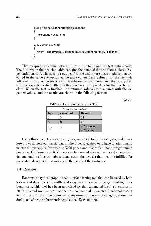
The interpreting is done between titles in the table and the test fixture code. The first row in the decision table contains the name of the test fixture class “Ex-ponentiationTest”. The second row specifies the test fixture class methods that are called in the same succession as the table columns are defined. For the methods followed by a question mark also the returned value is read and then compared with the expected value. Other methods set up the input data for the test fixture class. When the test is finished, the returned values are compared with the ex-pected values, and the results are shown in the following format:
Table 2FitNesse Decision Table after Test
ExponentiationTestbase exponent Result?2 5 324 2 16
1.5 22.2 expected2.25 actual
Using this concept, system testing is generalised to business logics, and there-fore the customers can participate in the process as they only have to additionally master the principles for creating Wiki pages and test tables, not a programming language. Furthermore, a Wiki page can be created also as the acceptance testing documentation since the tables demonstrate the criteria that must be fulfilled for the system developed to comply with the needs of the customer.
1.4. Ranorex
Ranorex is a typical graphic user interface testing tool that can be used by both testers and developers to swiftly and easy create new and manage existing func-tional tests. This tool has been appraised by the Automated Testing Institute: in 2010, this tool won its award as the best commercial automated functional testing tool in the NET and Flash/Flex sub-categories. In the entire category, it won the 2nd place after the aforementioned test tool TestComplete.
32 COMPUTER SCIENCE AND INFORMATION TECHNOLOGIES
LURaksti787-datorzinatne.indd 32LURaksti787-datorzinatne.indd 32 23.10.2012 12:02:2923.10.2012 12:02:29

Valdis Vizulis, Edgars Diebelis. Self-Testing Approach and Testing Tools
Customers that use this tool are globally known companies like Bosch, General Electrics, FujitsuSiemens, Yahoo, RealVNC etc.
Concept
Like all popular modern graphic user interface testing tools, also Ranorex’s concept is based on keyword-driven testing, recording the object, action and iden-tifier.
2.
4.
3.
5.
1.
6.
Test report Tested system EXE or DLL
C# or VB.NET
Figure 2. Ranorex Concept
1. Ranorex records the actions performed in the tested system.2. Ranorex transforms the recorded actions into C# or VB.NET code.3. To make the testing more convenient also for developers, the created C#
or VB.NET code can be edited also in the Visual Studio development environment.
4. An executable file or library is compiled from the code.5. The compiled testing “program” executes the recorded actions on the tes-
ted system.6. When the test is finished, a test report is generated in which the test sta-
tus is shown: successful or failed. For each test, detailed information can be viewed (Figure 3).
33
LURaksti787-datorzinatne.indd 33LURaksti787-datorzinatne.indd 33 23.10.2012 12:02:2923.10.2012 12:02:29

Fi gure 3. Ranorex Test Case Report
1.5. T-Plan Robot
T-Plan Robot is a flexible and universal graphic user interface testing tool that is built on image-based testing principles. This open source code tool does system testing from the user’s perspective, i.e. visual. Since the tool is able to test systems that cannot be tested with tools that are based on the object-oriented approach, in 2010 this tool won the ATI Automation Honors award as the best open source code automated functional testing tool in the Java sub-category. Among the company’s customers there are Xerox, Philips, Fujitsu-Siemens, Virgin Mobile and other.
Concept
Unlike many other typical functional testing tools, T-Plan Robot uses neither data- nor keyword-driven testing. Instead, it uses an image-based testing approach.
This approach lets the tool be independent from the technology which the tes-ted system is built or installed on. This tool is able to test any system that is depic-ted on the operating system’s desktop.
T-Plan Robot works with desktop images received from remote desktop techno-logies or other technologies that create images. For now, the tool only supports the testing of static images and the RFB protocol, which is better known with the name Virtual Network Computing. In future it is planned to add support for the Remote Desktop Protocol and local graphic card driver. [23]
In Figure 4, it can be seen how the testing runs using the client-server prin-ciple. The client and the server can cooperate through the network using the TCP/IP Protocol, or locally, using the desktop driver. T-Plan Robot works as a client that sends keyboard, mouse and clipboard events to the server. The tested system is located on the server, which sends to the client changes in the desktop image and the clipboard. T-Plan Robot is installed on the client’s system and runs on a Java virtual machine, which makes the tool independent from the platform.
34 COMPUTER SCIENCE AND INFORMATION TECHNOLOGIES
LURaksti787-datorzinatne.indd 34LURaksti787-datorzinatne.indd 34 23.10.2012 12:02:2923.10.2012 12:02:29

Valdis Vizulis, Edgars Diebelis. Self-Testing Approach and Testing Tools
Client machine
Client protocol using the TCP/IP or local desktop drivers
Tested machine
Operētājsistēma Opera�ng System
Servers – RFB, RDP...
Remote/local desktop
Remote/local
Keyboard, mouse and clipboard
events
Changes in the desktop image and
the clipboard
Opera�ng System
Java VM
T-Plan Robot n
Script interpreter
Robot
Clients RFB, RDP,
Java Test
Figure 4. T-Plan Robot Concept [23]
Tests are recorded by connecting to the remote desktop and running the tested system. At this moment T-Plan Robot registers the sent input data and the received changes in the desktop image or the clipboard and creates a test script.
The test is played back by executing the test script that contains the input data to be sent to the tested system. The received changes in the desktop image and the clipboard are compared with those registered when recording the test. At this mo-ment the tool’s image comparison methods are used.
The Client–Server architecture can be provided in three various ways [23]:1. One operating system with several desktops: only supported by Linux/
Unix as it lets run several VNC servers simultaneously;2. One computer wits several operating system instances: supported by all
operating systems because, using virtualisation technologies (e.g. Virtual-Box, VMware etc), the VNC server can be installed on the virtual computer;
3. Two separate computers: supported by all operating systems because when the computers are connected in a network, one runs as a client and the other as a server on which the tested system is installed.
1.6. Rational Functional Tester
The product offered by IBM, Rational Functional Tester (RFT), is an automated object-oriented approach automated functional testing tool that is one of the com-ponents in the range of lifecycle tools of the IBM Rational software.
35
LURaksti787-datorzinatne.indd 35LURaksti787-datorzinatne.indd 35 23.10.2012 12:02:2923.10.2012 12:02:29
Thi s tool is one of the most popular testing tools, but it has not won any ATI Automation Honors awards. In 2009 and 2010, it was a finalist among the best commercial automated functional and performance testing tools. It shows that now-adays there appear more and more new and efficient automated testing tools to which also RFT is giving up its positions in the market of testing tools.
Concept
IBM RFT was created to ensure automated functional and regress testing for the testers and developers who require premium Java, NET and web applications testing.
Java test scripts
VB.NET test scripts
Ra�onal Func�onal Tester client processes
Tested system
Inter-process communica�on
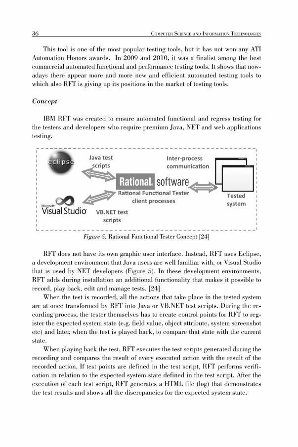
Figu re 5. Rational Functional Tester Concept [24]
RFT does not have its own graphic user interface. Instead, RFT uses Eclipse, a development environment that Java users are well familiar with, or Visual Studio that is used by NET developers (Figure 5). In these development environments, RFT adds during installation an additional functionality that makes it possible to record, play back, edit and manage tests. [24]
When the test is recorded, all the actions that take place in the tested system are at once transformed by RFT into Java or VB.NET test scripts. During the re-cording process, the tester themselves has to create control points for RFT to reg-ister the expected system state (e.g. field value, object attribute, system screenshot etc) and later, when the test is played back, to compare that state with the current state.
When playing back the test, RFT executes the test scripts generated during the recording and compares the result of every executed action with the result of the recorded action. If test points are defined in the test script, RFT performs verifi-cation in relation to the expected system state defined in the test script. After the execution of each test script, RFT generates a HTML file (log) that demonstrates the test results and shows all the discrepancies for the expected system state.
36 COMPUTER SCIENCE AND INFORMATION TECHNOLOGIES
LURaksti787-datorzinatne.indd 36LURaksti787-datorzinatne.indd 36 23.10.2012 12:02:3023.10.2012 12:02:30

Valdis Vizulis, Edgars Diebelis. Self-Testing Approach and Testing Tools
1.7. HP Unifi ed Functional Testing Software
HP Unified Functional Testing Software (HP UFTS), a tool offered by Hewlett Packard, is a premium quality automated functional and regress testing tool set that consists of two separate tools: HP Functional Testing Software (HP FTS) and HP Service Test Software (HP STS).
HP FTS is better known as HP QuickTest Professional (HP QTP) and formerly also as Mercury QuickTest Professional. HP FTS is based on HP QTP, but it has been supplemented with various extensions. It replaced a formerly popular tool, Mercury WinRunner, which was bought over by HP in 2006. Since most of the tool’s functionalities overlapped (or were taken over to) with HP FTS, in 2008 it was decided to terminate the support to the tool and it was recommended to transfer any previously recorded tests to HP FTS. HP STS, in turn, is a tool developed by HP itself, and it ensures automated functional testing of services with the help of activities diagrams. [25]
By merging the tools, HP obtained one of the most popular functional and re-gress testing tool in the world; in 2009, this tool won the ATI Automation Honors award as the best commercial automated functional testing tool, and in 2010 it was among the four finalists in the same category.
Concept
HP UFTS is a typical keyword- and data-driven testing tool that both makes the creation and editing of tests easier and ensures wide coverage of tests for tested systems.
To perform complete functional testing of a system, it is not sufficient to test the graphic user interface as the system functionality is not limited to solely the visual functionality. Many functionalities are “hidden” under the graphic user interface on the level of components. It can be especially seen in systems that run accord-ing to the principle “client-server”. These systems are called multi-level systems.
To ensure the testing of such systems, HP UFTS is based on the concept of multi-level testing (Figure 6). HP UFTS distributes multi-level testing in three levels [26]:
• graphic user interface testing;• services and components testing;• multi-level testing.
Graphic user interface testing is provided by HP FTS, which divides it into two levels: business processes testing and applications testing. Business pro-cesses testing can be done thanks to the test recording and playback functionality and keyword-driven testing that significantly simplify the creation and editing of tests and bring them closer to the business logics. Furthermore, to ensure quality testing of applications, HP FTS, with the integrated script creation and debugging
37
LURaksti787-datorzinatne.indd 37LURaksti787-datorzinatne.indd 37 23.10.2012 12:02:3023.10.2012 12:02:30
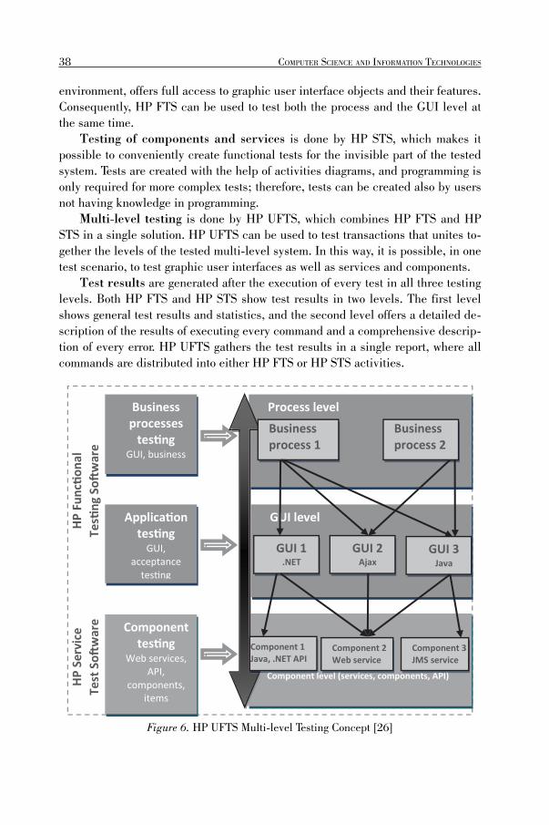
environment, offers full access to graphic user interface objects and their features. Consequently, HP FTS can be used to test both the process and the GUI level at the same time.
Testing of components and services is done by HP STS, which makes it possible to conveniently create functional tests for the invisible part of the tested system. Tests are created with the help of activities diagrams, and programming is only required for more complex tests; therefore, tests can be created also by users not having knowledge in programming.
Multi-level testing is done by HP UFTS, which combines HP FTS and HP STS in a single solution. HP UFTS can be used to test transactions that unites to-gether the levels of the tested multi-level system. In this way, it is possible, in one test scenario, to test graphic user interfaces as well as services and components.
Test results are generated after the execution of every test in all three testing levels. Both HP FTS and HP STS show test results in two levels. The first level shows general test results and statistics, and the second level offers a detailed de-scription of the results of executing every command and a comprehensive descrip-tion of every error. HP UFTS gathers the test results in a single report, where all commands are distributed into either HP FTS or HP STS activities.
HP F
unc�
onal
Te
s�ng
So�
war
e
Component level (services, components, API)
GUI level
Business processes
tes�ng GUI, business
Applica�on tes�ng
GUI, acceptance
tes�ng
Process level
Business process 1
Business process 2
GUI 1 .NET
GUI 2 Ajax
GUI 3 Java
C l
Component 1 Java, .NET API
l ( i
Component 2 Web service
API)
Component 3 JMS service
HP
Serv
ice
Test
So�
war
e Component tes�ng
Web services, API,
components, items
Figure 6. HP UFTS Multi-level Testing Concept [26]
38 COMPUTER SCIENCE AND INFORMATION TECHNOLOGIES
LURaksti787-datorzinatne.indd 38LURaksti787-datorzinatne.indd 38 23.10.2012 12:02:3023.10.2012 12:02:30

Valdis Vizulis, Edgars Diebelis. Self-Testing Approach and Testing Tools
As it can be seen in Figure 6, HP FTS enables the testing of both business pro-cesses and applications, making it possible to test the process and the GUI levels respectively in the tested system. Each business process is provided with one or more graphic user interfaces in various setups.
Graphic user interface is the visible part of the tested system that calls various components and services and receives from them the results to be showed to the users. As it can be understood, a majority of system functionalities are located on the system component level, and therefore HP STS offers the functional testing of various services, application interfaces, components and items.
From the aspect of testing concept, HP FTS does not offer a new approach, but in combination with HP STS this tool is able to offer different and diverse func-tional testing in three levels. This multi-level functional testing makes it possible to perform the testing prior to developing the graphic user interface, in this way allowing a faster development of the system and increasing the quality of compo-nents and services. Consequently, the overall quality of the graphic user interface is increased.
1.8. Selenium
Selenium is an open source code web application testing framework developed by OpenQA, and it consists of several testing tools. In the field of web applications testing, this framework has been a stable leader for more than five years, and last two years it has won the ATI Automation Honors award as the best open source code automated functional testing tool. A factor that contributes significantly to the advancement of this tool is that it is used in their testing projects by IT companies like Google, Mozilla, LinkedIn and others.
Concept
The Selenium framework consists of three different tools [27]:• Selenium IDE is a Selenium script development environment that makes
it possible to record, play back, edit and debug tests.• Selenium Remote Control is a basic module that can be used to record
tests in various programming languages and run them on any browser.• Selenium Grid controls several Selenium Remote Control instances to
achieve that tests can be run simultaneously on various platforms.For test creation, Selenium has developed its own programming language, Sele-
nese, which makes it possible to write tests in different programming languages. To execute tests, a web server is used that works as an agent between the browser and web requests, in this way ensuring that the browser is independent.
39
LURaksti787-datorzinatne.indd 39LURaksti787-datorzinatne.indd 39 23.10.2012 12:02:3023.10.2012 12:02:30
Selenium IDE
Selenium Grid
Selenium Remote Control
Tested system
Test script
1. 2.
3. 4.
5.
6.
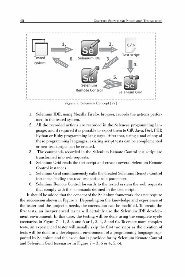
Figure 7. Selenium Concept [27]
1. Selenium IDE, using Mozilla Firefox browser, records the actions perfor-med in the tested system.
2. All the recorded actions are recorded in the Selenese programming lan-guage, and if required it is possible to export them to C#, Java, Perl, PHP, Python or Ruby programming languages. After that, using a tool of any of these programming languages, existing script tests can be complemented or new test scripts can be created.
3. The commands recorded in the Selenium Remote Control test script are transformed into web requests.
4. Selenium Grid reads the test script and creates several Selenium Remote Control instances.
5. Selenium Grid simultaneously calls the created Selenium Remote Control instances feeding the read test script as a parameter.
6. Selenium Remote Control forwards to the tested system the web requests that comply with the commands defined in the test script.
It should be added that the concept of the Selenium framework does not require the succession shown in Figure 7. Depending on the knowledge and experience of the tester and the project’s needs, the succession can be modified. To create the first tests, an inexperienced tester will certainly use the Selenium IDE develop-ment environment. In this case, the testing will be done using the complete cycle (scenarios in Figure 7 – 1, 2, 3 and 6 or 1, 2, 4, 5 and 6). To create more complex tests, an experienced tester will usually skip the first two steps as the creation of tests will be done in a development environment of a programming language sup-ported by Selenium and the execution is provided for by Selenium Remote Control and Selenium Grid (scenarios in Figure 7 – 3, 6 or 4, 5, 6).
40 COMPUTER SCIENCE AND INFORMATION TECHNOLOGIES
LURaksti787-datorzinatne.indd 40LURaksti787-datorzinatne.indd 40 23.10.2012 12:02:3023.10.2012 12:02:30

Valdis Vizulis, Edgars Diebelis. Self-Testing Approach and Testing Tools
2. Comparison of the Self-Testing Tool with other Testing Tools
The aim of this paper is to evaluate what features are offered by the self-testing tool compared to other tools and to identify directions for further development. It is difficult to determine from voluminous descriptions of tools what advantages and disadvantages a tool has compared to other tools. Also, it is rather difficult to assess which tool is best suited for a certain testing project. For this reason, it is important to compare the tools using certain criteria, which are analysed hereinafter and on the basis of which the tools will be compared.
2.1. Criteria for comparison
The criteria for comparison were selected on the basis of the possibilities of-fered by those seven tools looked at herein. The following aspects were taken into account by the author in selecting the criteria for comparison:
1. key features of testing;2. key features of automated testing tools;3. features offered by the compared tools.
Table 3 below lists the criteria used to compare testing tools and the question arising from the criteria, and answers to the questions are provided in the tool comparison tables (Table 4 and Table 5). To compare the self-testing tool and other tools looked at in this paper, the criteria described in Table 3 were used.
Table 3Criteria for Comparing Testing Tools
Comparison criteria QuestionTest method (TM) [28] What test methods are supported?Test automation approach (TAA) [29]
What test automation approaches are used?
Test automation framework (TAF) [30]
What test automation frameworks are used?
Testing level What test levels are supported?Functional testing Is functional testing supported?Non-functional testing What non-functional testing aspects are supported?Platform What operating systems are supported?Testable technology What technologies (usually programming languages) are
supported?Test recording and playback
Is test recording and automated reiterated playback provided?
41
LURaksti787-datorzinatne.indd 41LURaksti787-datorzinatne.indd 41 23.10.2012 12:02:3023.10.2012 12:02:30

Desktop applications testing
Is desktop applications testing provided?
Web applications testing Is web applications testing provided?Services testing Is services testing provided?Database testing Is it possible to test only the system database separately?Testing in production environment
Is testing in the production environment provided?
System user can create tests
Can system users without in-depth IT knowledge create tests?
Simultaneous running of several tests
Can tests be run simultaneously?
Performing simultaneous actions
Will the test performance not be disturbed if during the test simultaneous actions are performed?
Identifying the tested object
Is it able to tell apart the object to be tested from other objects of the operating system?
Test result analysis Is a test result analysis offered after the test?Test editing Is an editor for the created tests offered?Screenshots Are screenshots of the tested system acquired during the
recording/playback of the test?Control points Are control points offered?Object validation If modifications take place in the tested system, is object
validation provided?Object browser Is a browser/editor for objects of the tested system offered?Test log Is a test performance log created?Test schedule planner Is it possible to set the time for performing the test, e.g. at
night?Identifi cation of the end of command execution
Is the tool able to determine when the execution of the previous command has ended (and a certain waiting time is not used for this purpose)?
Plug-ins and extensions Is it possible to create own plug-ins and extensions to expand the tool’s functionality?
Developer What company or person has developed (owns) the testing tool?
Price How much the tool costs?Convenience of use (1-5) On the scale from 1 (very inconvenient) to 5 (very
convenient) – how convenient it is to create tests (author’s subjective assessment)?
Tool programming language
In what programming languages it is possible to create tests?
Client What companies use the tool in their testing projects?
42 COMPUTER SCIENCE AND INFORMATION TECHNOLOGIES
LURaksti787-datorzinatne.indd 42LURaksti787-datorzinatne.indd 42 23.10.2012 12:02:3023.10.2012 12:02:30

Valdis Vizulis, Edgars Diebelis. Self-Testing Approach and Testing Tools
2.2. Comparison results
To assess every comparison criteria determined, information obtained from the tool’s official website and other trusted websites, specifications and help windows and from practical use of the test tools was used to make sure that they comply with the respective criteria.
To ensure maximum objectivity of the comparison results, the author tried, to the extent possible, avoid using his own subjective judgment and base the com-parison on whether the tool offers a feature or not. To this end, the criteria in the comparison provided in Table 4 and table 5 were evaluated using the following three answers:
• Yes – it means that the tool supports the functionality referred to in the criteria;
• Partially – it means that the tool partially supports the functionality re-ferred to in the criteria;
• No – it means that the tool does not support the functionality referred to in the criteria.
The paper contains two comparison tables: Table 4 provides a summary on the comparison criteria that the self-testing tool supports, and Table 5 provides a sum-mary on the comparison criteria that the self-testing tool does not currently support.
43
LURaksti787-datorzinatne.indd 43LURaksti787-datorzinatne.indd 43 23.10.2012 12:02:3023.10.2012 12:02:30
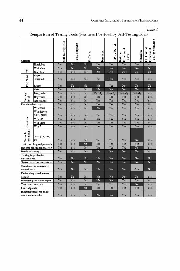
Table 4Comparison of Testing Tools (Features Provided by Self-Testing Tool)
44 COMPUTER SCIENCE AND INFORMATION TECHNOLOGIES
LURaksti787-datorzinatne.indd 44LURaksti787-datorzinatne.indd 44 23.10.2012 12:02:3023.10.2012 12:02:30

Valdis Vizulis, Edgars Diebelis. Self-Testing Approach and Testing Tools
Table 5Comparison of Testing Tools (Features not Provided by Self-Testing Tool)
45
LURaksti787-datorzinatne.indd 45LURaksti787-datorzinatne.indd 45 23.10.2012 12:02:3123.10.2012 12:02:31

The next table (Table 6) shows the additional criteria for comparing the tools that were not included in the previous tool comparison tables.
Table 6Comparison of Testing Tools 2
Testing Tool DeveloperPrice (EUR)
Con-veni-ence
ClientTool ‘s programming language
Self-testing tool
Datorikas institūts DIVI
* 5 * C#
TestComplete SmartBear Software
~ 1 400 3
Adobe, Corel, Falafel Software, ARUP Laboratories, QlikTech u.c.
VBScript, Jscript, C++Script, C#Script, DelphiScript
FitNesse Robert C. Martin
Free 4 * Java
Ranorex Ranorex ~ 1 190 3
Bosch, General Electrics, FujitsuSiemens, Yahoo, RealVNC u.c.
C++, Python, C#, VB.NET
T-Plan Robot T-Plan Free 3Xerox, Philips, FujitsuSiemens, Virgin Mobile u.c.
Java
Rational Functional Tester
IBM2 700 – 11 000
4 * Java, VB.NET
Selenium OpenQA Free 3Google, Mozilla, LinkedIn u.c.
C#, Java, Perl, PHP, Python, Ruby
HP Unifi ed Functional Testing Software
Hewlett Packard
3 000 – 10 000
4 * VBScript, C#
* – no/not available
3. Conclusions
To compare the seven testing tools, the author had to analyse not only their builds but also their concepts in order to assess objectively what are the pros and cons of the self-testing tool and what could be the directions for its further
46 COMPUTER SCIENCE AND INFORMATION TECHNOLOGIES
LURaksti787-datorzinatne.indd 46LURaksti787-datorzinatne.indd 46 23.10.2012 12:02:3123.10.2012 12:02:31

Valdis Vizulis, Edgars Diebelis. Self-Testing Approach and Testing Tools
development. From the comparison of the seven tools, the following conclusions can be drawn:
• The self-testing tool, TestComplete and FitNesse, thanks to the possibility to access the internal structure of the tested system, offers the grey-box testing (self-testing tool offers also white-box testing) method, which makes it possible to test the system more detailed. The other testing tools employ the black-box testing method;
• Among the seven tools looked at in this paper, only one uses an image-based approach as the test automatisation approach. All the others use the object-oriented approach. Consequently, it can be concluded that the object-oriented approach is the most popular for the automatisation of tests;
• In comparison to the other tools described in this paper, the self-testing tool provides for a wide range of testing levels, as TestComplete is the only one that, in addition to unit, integration, regress, functional and acceptance testing, offers also stress and load testing, while the others are limited to only three testing levels. It has to be noted that, considering the ability of self-testing to run parallel tests, it would be comparatively simple to imple-ment the stress and load testing support also in the self-testing tool.
• Of the test automation tools dealt with in this paper, FitNesse is the only one that does not provide the test recording and playback functionality. Instead of it, a convenient creation of tests in table format is offered.
• Just a few testing tools offer such features included in the self-testing tool as database testing, simultaneous execution of tests and parallel actions during testing, whereas almost all testing tools offer the identification of the tested object, test result analysis and the adding of control points to the test;
• Only the self-testing tool offers the possibility to run testing in the pro-duction environment and the possibility to create tests for users without in-depth IT knowledge;
• The self-testing tools and Ranorex are the only one that do not offer the feature of adding existing or new plug-ins and extensions;
• The self-testing tool is not the only one that requires additional resources prior to creating tests, as also for FitNesse test fixtures must be developed for successful performance of the tests.
A number of the criteria listed in table 5 and currently not supported by the self-testing tool can be implemented through comparatively minor improvements to the tool. For example, to achieve that the self-testing tool supports performance testing, just a new test point that would control the performance of action execution needs to be implemented.
Self-testing is a new and original approach that does not lag behind other tools, and in some areas it is undoubtedly even better.
47
LURaksti787-datorzinatne.indd 47LURaksti787-datorzinatne.indd 47 23.10.2012 12:02:3123.10.2012 12:02:31

IEGULDĪJUMS TAVĀ NĀKOTNĒ
This work has been supported by the European Social Fund within the project «Support for Doctoral Studies at University of Latvia».
References
1. Wikiversity. [Online] [Quoted: 24 January, 2011] http://en.wikiversity.org/wiki/Software_testing/history_of_testing.
2. Bičevska, Z., Bičevskis, J.: Smart Technologies in Software Life Cycle. In: Münch, J., Abra-hamsson, P. (eds.) Product-Focused Software Process Improvement. 8th International Conference, PROFES 2007, Riga, Latvia, July 2-4, 2007, LNCS, vol. 4589, pp. 262-272. Springer-Verlag, Berlin Heidelberg (2007).
3. Rauhvargers, K., Bicevskis, J.: Environment Testing Enabled Software - a Step Towards Execution Context Awareness. In: Hele-Mai Haav, Ahto Kalja (eds.) Databases and Information Systems, Selected Papers from the 8th International Baltic Conference, IOS Press vol. 187, pp. 169-179 (2009)
4. Rauhvargers, K.: On the Implementation of a Meta-data Driven Self Testing Model. In: Hruška, T., Madeyski, L., Ochodek, M. (eds.) Software Engineering Techniques in Progress, Brno, Czech Republic (2008).
5. Bičevska, Z., Bičevskis, J.: Applying of smart technologies in software development: Automated version updating. In: Scientific Papers University of Latvia, Computer Science and Information Technologies, vol .733, ISSN 1407-2157, pp. 24-37 (2008)
6. Ceriņa-Bērziņa J.,Bičevskis J., Karnītis Ģ.: Information systems development based on visual Domain Specific Language BiLingva. In: Accepted for publication in the 4th IFIP TC2 Central and East European Conference on Software Engineering Techniques (CEE-SET 2009), Krakow, Poland, Oktober 12-14, 2009
7. Ganek, A. G., Corbi, T. A.: The dawning of the autonomic computing era. In: IBM Systems Journal, vol. 42, no. 1, pp. 5-18 (2003)
8. Sterritt, R., Bustard, D.: Towards an autonomic computing environment. In: 14th International Workshop on Database and Expert Systems Applications (DEXA 2003), 2003. Proceedings, pp. 694 - 698 (2003)
9. Lightstone, S.: Foundations of Autonomic Computing Development. In: Proceedings of the Fourth IEEE international Workshop on Engineering of Autonomic and Autonomous Systems, pp. 163-171 (2007)
10. Diebelis, E., Takeris, V., Bičevskis, J.: Self-testing - new approach to software quality assurance. In: Proceedings of the 13th East-European Conference on Advances in Databases and Informa-tion Systems (ADBIS 2009), pp. 62-77. Riga, Latvia, September 7-10, 2009.
11. Bičevska, Z., Bičevskis, J.: Applying Self-Testing: Advantages and Limitations. In: Hele-Mai Haav, Ahto Kalja (eds.) Databases and Information Systems, Selected Papers from the 8th Inter-national Baltic Conference, IOS Press vol. 187, pp. 192-202 (2009).
12. Diebelis, E., Bičevskis, J.: An Implementation of Self-Testing. In: Proceedings of the 9th In-ternational Baltic Conference on Databases and Information Systems (Baltic DB&IS 2010), pp. 487-502. Riga, Latvia, July 5-7, 2010.
13. Diebelis, E., Bicevskis, J.: Test Points in Self-Testing. In: Marite Kirikova, Janis Barzdins (eds.)
48 COMPUTER SCIENCE AND INFORMATION TECHNOLOGIES
LURaksti787-datorzinatne.indd 48LURaksti787-datorzinatne.indd 48 23.10.2012 12:02:3123.10.2012 12:02:31

Valdis Vizulis, Edgars Diebelis. Self-Testing Approach and Testing Tools
Databases and Information Systems VI, Selected Papers from the Ninth International Baltic Con-ference. IOS Press vol. 224, pp. 309-321 (2011).
14. Automated Software Testing Magazine. [Online] [Quoted: 20 January, 2011] http://www.automa-tedtestinginstitute.com/home/index.php?option=com_conten t&view=article&id=1276&Itemid=122.
15. Automated Testing Institute. [Online] [Quoted: 15 January, 2011] http://www.automatedtestin-ginstitute.com.
16. Verify/ATI Conference. [Online] [Quoted: 2011. gada 12. maijā.] http://www.verifyati.com.17. ATI Automation Honors. [Online] [Quoted: 20 January, 2011] http://www.automatedtestinginsti-
tute.com/home/index.php?option=com_conten t&view=article&id=1262&Itemid=131.18. ATI Schedule & Selection Process. [Online] [Quoted: 16 January, 2011] http://www.automa-
tedtestinginstitute.com/home/index.php?option=com_content&view=article&id=1283&Itemid=156.
19. SmartBear Software. [Online] [Quoted: 15 December, 2010] http://www.automatedqa.com/pro-ducts/testcomplete/.
20. Testing Geek - FitNesse Introduction. [Online] [Quoted: 3 April, 2011] http://www.testinggeek.com/index.php/testing-tools/test-execution/95-fitnesse-introduction.
21. Wikipedia - Wiki. [Online] [Quoted: 10 April, 2011] http://en.wikipedia.org/wiki/Wiki.22. Wikipedia. [Online] [Quoted: 10 April, 2011] http://en.wikipedia.org/wiki/FitNesse.23. T-Plan Robot Enterprise 2.0 Tutorial. [Online] [Quoted: 17 April, 2011] http://www.t-plan.com/
robot/docs/tutorials/v2.0/index.html.24. IBM Help System. [Online] [Quoted: 19 April, 2011] http://publib.boulder.ibm.com/infocenter/
rfthelp/v7r0m0/index.jsp?topic=/com.ibm.rational.test.ft.proxysdk.doc/topics/c_pr_architectu-re.html.
25. HP - Looking for Mercury Interactive? [Online] [Quoted: 9 May, 2011] https://h10078.www1.hp.com/cda/hpms/display/main/hpms_content.jsp?zn=bto&cp=1-10^36653_4000_100__&jumpid= reg_R1002_USEN#.
26. HP Unified Functional Testing software. [Online] [Quoted: 6 May, 2011] https://h10078.www1.hp.com/cda/hpms/display/main/hpms_content.jsp?zn=bto&cp=1-11-127-24^1352_ 4000_100__.
27. Selenium Web Application Testing System. [Online] [Quoted: 30 April, 2011] http://seleniumhq.org/.
28. Pressman Roger, S. Software Engineering - A Practioner’s approach 5th edition. New York : The McGraw-Hill Companies, Inc., 2001.
29. T-Plan Robot - Image Based vs Object Oriented Testing. [Online] [Quoted: 3 April, 2011] http://www.t-plan.com/robot/docs/articles/img_based_testing.html
30. Automatic Testing Frameworks. [Online] [Quoted: 19 April, 2011] http://www.automatictes-tingframeworks.com/?q=test_automation_framework.
49
LURaksti787-datorzinatne.indd 49LURaksti787-datorzinatne.indd 49 23.10.2012 12:02:3123.10.2012 12:02:31

Data Acquisition from Real World Objects based on Nonuniform Signal Sampling and Processing
Kaspars Sudars
University of Latvia, Faculty of Computing, Institute of Electronics and Computer Science
The paper summarizes obtained research and practical results reported in the author’s doctoral Thesis “Data Acquisition from Real World Objects”. Work is focused on methods and algorithms for data acquisition from real world objects, and it is based on the theory of non-traditional Digital Signal Processing, includ-ing non-uniform sampling and pseudo-randomized quantizing. That leads to ob-taining data simultaneously from an increased number of data sources, to widen-ing the frequency range and to significant complexity reductions. In particular, research has been done in the directions of: (1) asymmetric data compression/reconstruction; (2) data acquisition from sources in the GHz frequency range; (3) rational acquisition of impedance data; (4) data acquisition based on signal and sine wave reference function crossings. Microelectronic implementation of the research results is considered. In particular, FPGA implementation of a Fast-DFT processor has been developed and tested.
Keywords. Data acquisition, Nonuniform signal sampling, Impedance mea-surements, DASP
1. Introduction
Motivation for research in the area of data acquisition for computer systems
Massive data acquisition from real life objects and supplying computers with this information in an effective way evidently is vital to realizing full potential of computer system applications in many areas. Various types of sensors are used for obtaining information from objects of natural or technical origin. Most of them convert the primary information into continuous-time or analog sig-nals. Data acquisition (DAQ) from only this type of sensors is considered. As the acquired data are to be given as discrete quantities, the analog sensor sig-nals have to be digitized to obtain their representations in the digital domain. Usually the classic Digital Signal Processing (DSP) technology is used for this.
SCIENTIFIC PAPERS, UNIVERSITY OF LATVIA, 2012. Vol. 787COMPUTER SCIENCE AND INFORMATION TECHNOLOGIES 50–78 P.
LURaksti787-datorzinatne.indd 50LURaksti787-datorzinatne.indd 50 23.10.2012 12:02:3123.10.2012 12:02:31

Kaspars Sudars. Data Acquisition from Real World Objects based on Nonuniform Signal ..
This approach, based on the assumption that digitizing is based on the classi-cal sampling and quantizing concepts, leads to significant narrowing of the digital domain, to using of more expensive analog signal processing methods and techni-cal means for performing signal processing in the high and ultra high frequency range. It means that this approach negatively impact data acquisition technologies and limits their application range. The research described in this summary is moti-vated by the importance of achieving progress in the direction of computer system applications in the wide area of Information Technologies related to computer sys-tem interaction with real world biological and industrial objects.
Research goal and the basic problems that have to be resolved
Research activities of work target reaching the goal of discovering innovative methods for massive data acquisition from real life objects and effective supplying computers with this information. That evidently is vital for realizing full potential of computer system applications in many areas. The research is focused on resolu-tion of the following basic problems that have been indicated at the beginning as the most essential:
• Too high DAQ system complexity;• Relatively small quantity of sensors that typically can be connected to in-
puts of a single DAQ system;• Limited number of channels for simultaneous data acquisition in parallel; • Power consumption of DAQ systems, often limiting the duration of their
autonomous performance time.
Basic tasks
To achieve progress in these directions, the following tasks are addressed: 1. Research focused on development of innovative methods and algorithms
for complexity-reduced DAQ paying attention, in particular, on the fol-lowing:
• Combining data acquisition with signal specific digital pre-pro-cessing;
• Reduction of power consumption;• Increasing the number of sensors that can be connected to a single
DAQ system at least up to 100;• Compression of acquired data.
2. Development of algorithms and computer programs for sensor data trans-fer to computers.
3. Experimental investigations of the developed problem solutions, mostly by computer simulations in MATLAB environment.
4. Description of the developed DAQ structures in VHDL.
51
LURaksti787-datorzinatne.indd 51LURaksti787-datorzinatne.indd 51 23.10.2012 12:02:3123.10.2012 12:02:31

Approach to resolution of the considered problems
To reach the goal a flexible approach to complexity-reduced multi-channel data acquisition from a large quantity of sensors has been used. The developed methods, systems and algorithms for data acquisition from wideband, event timing and large distributed clusters of signal sources are discussed with emphasis on data gather-ing from a large quantity of signal sources. Special signal digitizing techniques, including pseudo-randomized multiplexing, time-to-digital conversions and signal sample value taking at time instants when the input signal crosses a sinusoidal reference function, are used for that. Development of the discussed massive data acquisition systems is based on the knowledge accumulated over a long period of time in the area of Digital Alias-free Signal Processing.
2. DAQ Systems for Information Gathering and Supplying to Computers
Relatively many various DAQ systems are currently produced and offered by many companies. On the other hand most of them actually are operating on the basis of a few basic DAQ principles that can be considered as classic as they have remained unchanged for a long time. Therefore performance of the existing DAQ systems mainly depends on the currently achieved perfection of the involved mi-croelectronic elements.
Analysis of the currently used data acquisition system specifics reveals some essential facts and leads to the following generalized conclusions:
1. DAQ systems mostly belong to one of two basic types of DAQ systems: (1) multi-channel systems for DAQ based on multiplexing inputs to a central ADC connected via interface to a computer; (2) multi-channel systems for so-called simultaneous DAQ using a separate ADC in every input channel.
2. DAQ functions usually are considered as input signal conditioning, analog-to-digital conversions and transmitting the digital signals, obtained from all inputs, to the computer. Processing of data more often than not is the responsibility of the host computer.
3. The essential function of signal digitizing usually is performed on the basis of the classical concepts of uniform periodic sampling (Shannon sampling theorem) and fixed-threshold quantizing.
4. The sampling rate of for DAQ systems based on multiplexing inputs to a central ADC directly depends on the clock frequency at which the multi-plexer is switched and the rate of sampling signals in each input channel is inversely proportional to the number of inputs.
5. Consequently the quantity of DAQ system inputs usually is restricted to relatively small numbers, usually up to 16. More complicated systems con-
52 COMPUTER SCIENCE AND INFORMATION TECHNOLOGIES
LURaksti787-datorzinatne.indd 52LURaksti787-datorzinatne.indd 52 23.10.2012 12:02:3123.10.2012 12:02:31

Kaspars Sudars. Data Acquisition from Real World Objects based on Nonuniform Signal ..
tain a hierarchy of multiplexers. In this case there might be more inputs however this type of DAQ systems then can be used only for data acquisi-tion from low-frequency sources.
6. Using a separate ADC in every input channel allows avoiding these re-strictions. Therefore this type of DAQ systems can be used for obtain-ing data from high frequency signal sources. The factors limiting their applications are relatively high complexity (ADC in every channel) and multiplexing of ADC output signals needed for transmitting them sequen-tially to the host computer. The quality of developed and produced DAQ systems improve all the time, however this progress is mostly based on the achievements in the area of semiconductor device development and production technologies.
The last conclusion is true for most of the currently produced DAQ equipment. On the other hand, there have been various R&D efforts addressing the problem of data acquisition under conditions more demanding than usual.
In particular, the applicability of NU sampling and low-bit rate quantizing has been investigated over a long period of time and this approach is directly related to DAQ functions [15, 16, 33, 34]. These methods and algorithms are applicable for achieving a number of essential advantages, such as performing of DAQ in a wide frequency range, elimination the dependency of the sampling rate in a chan-nel on the quantity of channels in a system, data compression/reconstruction, reducing the complexity of DAQ systems and others. That leads to the following conclusions:
1. The currently used classical theory covering signal digitizing (sampling and quantizing) and digital representation of analog signals is not ex-clusive. These signal conversion operations can be performed in various ways, based on the signal digitizing theory developed in a few past dec-ades, including theory of randomized signal processing, NU sampling and quantizing and DASP.
2. To achieve progress in the area of DAQ, efforts have to be put in this work basically in the directions of developing methods and algorithms for application-specific DAQ.
3. Selecting and using the most effective type of digital representation of analog input signals is really important for that.
4. Data pre-processing in many cases should be included in the list of func-tions to be fulfilled by a DAQ system as algorithms for parallel processing of raw digital signals can be developed and used at that stage for effective data representation and compression.
Reduction of power consumption, simplification of system hardware, simplifi-cation of algorithms for acquired data pre-processing and enlargement of system channel quantity, accurate signal acquisition are still very desirable for DAQ systems.
53
LURaksti787-datorzinatne.indd 53LURaksti787-datorzinatne.indd 53 23.10.2012 12:02:3123.10.2012 12:02:31

3. Data Acquisition Based on NU Sampling: Achievable Advantages and Involved Problems
Periodic sampling is currently the most used and widespread sampling method. However there are other methods for sampling, specifically, NU sampling. The achievable advantages and application potential of this approach are based on ex-ploitation of the capabilities offered by the NU sampling procedure carried out in the process of the sensor signal digitizing [15, 16, 23, 33, 34, 38].
Whenever continuous time signals are digitized and then processed on the ba-sis of DSP, the sampling rate fs of the used periodic sampling limits the bandwidth of the original analog signals. Then the restrictions, defined by the Sampling theo-rem, have to be satisfied to avoid the uncertainty due to the fact that all frequencies belonging to the sequence: fo; fs±fo; 2fs±fo; 3fs±fo;... nfs±fo are indistinguishable.
However that is true only under the conditions of periodic sampling. The situ-ation is different whenever DAQ is based on the lately developed signal digitizing theory, including theory of randomized signal processing, NU sampling and quan-tizing and DASP. Specifically, the basic effect achieved by using NU sampling is avoiding aliasing. This achievable capability is very important for DAQ.
Problems related to NU based DAQ are investigated. The most significant is the problem of cross-interference (CI) between signal spectral components occur-ring whenever the signal sample values are taken at non-equidistant time instants. Impact of CI on DAQ is taken into account and CI is suppressed.
On the other hand, the obtained results show that various specific advantages and benefits, valuable for practical applications, can be obtained by exploiting NU sampling techniques. Several methods of this kind are considered further.
Data acquisition from high frequency signal sources
As proper application of NU sampling leads to elimination of aliasing, this spe-cific approach to signal sampling can be used to enlarge the frequency range where information carried by high frequency analog sensor signals can be represented by digital data (for example, in cases of signal demodulations).
A structure of DAQ systems based on NU is considered. It can be used for data acquisition directly from high frequency signal sources if operation of the used ADCs is based on quantizing signal sample values taken from the input signal at time instants dictated by a NU sampling point process. In such a case the usage of the additive sampling point process is usually preferable. The upper frequency of the signal spectrum sometimes can exceed the mean sampling rate several times. This makes it possible to acquire data in a wide frequency range extending up to few GHz. However the data obtained under these conditions then must be treated with the specifics of NU sampling taken into account [12, 13, 17].
54 COMPUTER SCIENCE AND INFORMATION TECHNOLOGIES
LURaksti787-datorzinatne.indd 54LURaksti787-datorzinatne.indd 54 23.10.2012 12:02:3123.10.2012 12:02:31

Kaspars Sudars. Data Acquisition from Real World Objects based on Nonuniform Signal ..
Increasing the quantity of input channels
The structure of the DAQ system used for data acquisition from a multitude of sensors is based on multiplexing of analog signals. The difference between the traditional structures of this type and this one is in operation of the multiplexer. Whenever it connects inputs to the ADC periodically, the number of inputs is lim-ited by the achievable multiplexer switching rate as the sampling rate of each input then is n times lower, where n is the number of inputs. Replacing the periodic multiplexer switching by randomized allows using the total bandwidth of channels more efficiently. Therefore that makes it possible to increase the number of inputs several times. [14].
Data acquisition at object testing
Exploiting NU sampling techniques and gaining advantages on that basis is a considerably less complicated task under conditions typical for the cases where data are acquired from some biomedical or industrial objects that are being tested. Then the information that has to be obtained is related to the characteristics and properties of the object and the signals taken off the respective object during the tests carry it. These signals reflect reaction of the object on some specific excita-tion signals that are used. The fact that data acquisition then is performed under conditions where the test signal characteristics, including its spectrum, are given is very useful. Taking this information into account makes it possible to reduce the complexity of the following data processing process significantly. Using of this a priori information leads to substantial simplification of the algorithms. All cross-interference coefficients then can be pre-calculated, matrix C of their values also can be composed and inverted so that all elements �ij of the inverted matrix inv(C) also could be pre-calculated. Therefore the Fourier coefficients in this case can be calculated directly. That dramatically simplifies and speeds-up the involved calculations.
Using of this approach for data acquisition in the specific case of bioimpedance signal analysis in a wide frequency range of the test signals (up to a few GHz) is described. [35].
Fault tolerant data acquisition
Suppose data are acquired under conditions where the spectra of the involved processes are restricted at relatively low frequencies. Then application of NU sam-pling is not needed and data might and should be acquired at periodically repeating time instants. Attention is drawn to the possibility of improving the performance of the data acquisition system on the basis of NU sampling even under these condi-tions if it is needed to protect this system against unpredictable explosive noise bursts. Then the concept of NU sampling and specific data processing typical for NU sampling still proves to be quite useful.
55
LURaksti787-datorzinatne.indd 55LURaksti787-datorzinatne.indd 55 23.10.2012 12:02:3123.10.2012 12:02:31

Time diagrams shown in Figure 1 illustrate the data acquisition process un-der normal conditions in Figure 1(a) and under the impact of noise bursts in Figure 1(b).
Figure 1. Impact of noise bursts on signals: (a) periodically sampled continuous sig-nal, (b) the same signal with bursts of lost data and the recovered parts of faulted signal.
The idea of improving fault tolerance on this basis is simple. The essence of it is as follows: to improve fault tolerance on the basis of the NU sampling concept, the data should be acquired periodically as usual and facilities usually used for processing of nonuniformly acquired data should be added to the system and used for data reconstruction [12, 13, 17]. This means that under normal data acquisition conditions redundant equipment would be used. The role of this equipment would be to recover the data lost under impact of the noise bursts.
Asymmetric data compression/reconstruction
Data compression function plays a significant role at DAQ. Essential are the advantages related to data compression obtainable if proper NU sampling proce-dures are used.
At standard data compression/reconstruction data are processed twice to com-press and decompress them. Naturally that requires using of computing resources twice and that takes time. Using of the NU sampling procedures makes it possi-ble to reduce the volume of data representing the respective input sensor signals simply by taking out some quantity of the signal sample values or perform other simple operation. It means that in this case no calculations are made at data com-pression. The computational burden related to reconstruction of the compressed
56 COMPUTER SCIENCE AND INFORMATION TECHNOLOGIES
LURaksti787-datorzinatne.indd 56LURaksti787-datorzinatne.indd 56 23.10.2012 12:02:3123.10.2012 12:02:31
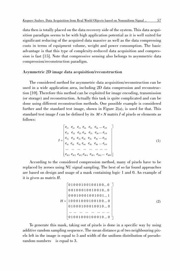
Kaspars Sudars. Data Acquisition from Real World Objects based on Nonuniform Signal ..
data then is totally placed on the data recovery side of the system. This data acqui-sition paradigm seems to be with high application potential as it is well suited for significant reducing of the acquired data massive as well as the data compressing costs in terms of equipment volume, weight and power consumption. The basic advantage is that this type of complexity-reduced data acquisition and compres-sion is fast [15]. Note that compressive sensing also belongs to asymmetric data compression/reconstruction paradigm.
Asymmetric 2D image data acquisition/reconstruction
The considered method for asymmetric data acquisition/reconstruction can be used in a wide application area, including 2D data compression and reconstruc-tion [10]. Therefore this method can be exploited for image encoding, transmission (or storage) and reconstruction. Actually this task is quite complicated and can be done using different reconstruction methods. One possible example is considered further and the standard test image, shown in Figure 2(a), is used for that. This standard test image I can be defined by its NM matrix I of pixels or elements as follows:
11 12 13 14 15 16 1
21 22 23 24 25 26 2
31 32 33 34 35 36 3
41 42 43 44 45 46 4
1 2 3 4 5 6
...
...
...
...... ... ... ... ... ... ... ...
...
N
N
N
N
M M M M M M MN
e e e e e e ee e e e e e ee e e e e e e
Ie e e e e e e
e e e e e e e
(1)
According to the considered compression method, many of pixels have to be replaced by zeroes using NU signal sampling. The best of so far found approaches are based on design and usage of a mask containing logic 1 and 0. An example of it is given as matrix H.
0 1 0 0 0 1 0 0 1 0 0 1 0 0... 00 0 1 0 0 0 1 0 0 1 0 0 1 0... 00 0 0 1 0 0 0 1 0 0 1 0 0 1 ... 11 0 0 0 1 0 0 0 1 0 0 1 0 0 ... 00 1 0 0 0 1 0 0 0 1 0 0 1 0 ... 0... ... ... ... ... ... ... ...0 1 0 0 1 0 0 0 1 0 0 0 1 0 ... 0
H
(2)
To generate this mask, taking out of pixels is done in a specific way by using additive random sampling sequence. The mean distance μ of two neighbouring pix-els left in the image is equal to 5 and width of the uniform distribution of pseudo-random numbers � is equal to 3.
57
LURaksti787-datorzinatne.indd 57LURaksti787-datorzinatne.indd 57 23.10.2012 12:02:3123.10.2012 12:02:31

The compressed image is obtained in a very simple and fast way, just by using logic or scalar multiplication of generated mask matrix with the image matrix:
12 16 19 1
23 27 2
34 38 3
41 45 49 4
2 5 9
0 0 0 0 0 0 ...0 0 0 0 0 0 0...0 0 0 0 0 0 0 ...
0 0 0 0 0 0 ...... ... ... ... ... ... ...0 0 0 0 0 0 ...
N
N
Nc
N
M M M MN
e e e ee e e
e e eI I H
e e e e
e e e e
(3)
The obtained sparse image after losing 80.27% of its pixels is shown in Figure 2(b). Evidently image compression performed in such a way is a quite inexpensive and technically effective operation. The complexity of this type of image compres-sion is much lower than the complexity of the usually exploited rather complicated standard image compression algorithms. That apparently represents a significant advantage of the proposed and described 2D data compression algorithm.
Reconstruction of the compressed image
Two approaches of sparse image reconstruction were considered and studied. Both of them have a common first recovery stage. The result obtained after this stage is shown in Figure 2(c). According to the suggested reconstruction method, part of all unknown image pixels can be calculated at this stage by processing its subsequent pixel values if these are known. In this particular sampling case, the maximum count of the known pixels in close proximity (considering 2D 4-pixel con-nectivity case) can be 2. These pixels can be approximately calculated as follows:
, 1, , 1ˆ 0.5( ),mn l m n m ne e e for the left side estimates
, 1, , 1ˆ 0.5( ),mn r m n m ne e e for the right side estimates(4)
Where m = 1, 2, 3 …M, n = 1, 2, 3 …N. The matrix of the recovered image pixel values after the first reconstruction cycle is the following:
11 12 13 15 16 17 19 1
22 23 24 26 27 28 2
33 34 35 37 38 39 31
41 42 44 45 46 48 49 4
1 2 4 5 8 9
ˆ ˆ ˆ ˆ0 0 ...ˆ ˆ ˆ ˆ0 0 0 ...
ˆ ˆ ˆ ˆ0 0 0 ...ˆˆ ˆ ˆ ˆ0 0 ...
... ... ... ... ... ... ... ... ... ... ...ˆ ˆ ˆ0 0 0 ...
N
N
Nr
N
M M M M M M MN
e e e e e e e ee e e e e e e
e e e e e e eI
e e e e e e e e
e e e e e e e
(5)
At the next stages this process can be continued iteratively. All the pixel values are estimated in this way after a few cycles and the full image is recovered.
The average relative error, obtained in this particular case at image reconstruc-tion performed in accordance to the described method, is equal to 0.1648 %.
58 COMPUTER SCIENCE AND INFORMATION TECHNOLOGIES
LURaksti787-datorzinatne.indd 58LURaksti787-datorzinatne.indd 58 23.10.2012 12:02:3123.10.2012 12:02:31

Kaspars Sudars. Data Acquisition from Real World Objects based on Nonuniform Signal ..
The second considered reconstruction method is based on application of SEC-OEX method. That leads to the result shown in Figure 2(e). In this particular case, the average relative error of image recovery is 0.3147 %, what actually is worse than the result obtained by the previous method. While this larger error can be explained by the particularities of the processed test image signals, image recon-struction based on the SECOEX method is much more complicated and more time consuming in comparison with the developed method.
Figure 2. Example of asymmetric DAQ compression/reconstruction: (a) the original image by size 512×512 pixels; (b) sparse image after losing 80.27% of its pixels; (c) the image recovered at the first recovery stage; (d) image recovered by calculating unknown pixels from their neighbours and (e) recovered image obtained on the basis of SECOEX
method.
59
LURaksti787-datorzinatne.indd 59LURaksti787-datorzinatne.indd 59 23.10.2012 12:02:3223.10.2012 12:02:32

The asymmetric 2D data acquisition/reconstruction has significant advantages for application cases where computational power is limited and transmitting of the acquired data is expensive in terms of spent time, memory and equipment resources.
The applicability of this method has been widened to cover also processing of colour images. An experimental system has been developed and made for studies of the described image compression method.
Wideband signal digitizing in enlarged dynamic range
The frequency range, where the currently available 10 to 12 bit ADCs are ap-plicable, often is not wide enough. On the other hand, the dynamic range of the ADCs, applicable for analog-digital conversions in GHz frequency range, is limited by the achievable quantization bit rate usually not exceeding 4 bits [19, 41]. These typical problems, arising at attempts to convert analog signals into their digital counterparts in a wide frequency range extending up to GHz frequencies, are stud-ied and specific approaches to resolution of them is suggested further.
Combining precise and low-bit very fast sampling
Combining precise and low-bit very fast sampling, in particular, significantly widen the area where DAQ can be performed in GHz frequency range by using low bit rate ADC. This type of signal sampling/reconstruction scheme is shown in Figure 3. The sampling operation in this case is based on adding to the precise ADC another low-bit rate one, which has to be very fast.
Figure 3. Structure of the electronic systems used for iterative reconstruction of signal waveforms, when signal is sampled using two ACDs in parallel.
Reconstruction of signal waveforms in this case is based on iterative filtering procedure. Results of 4 bit fast periodic sampling are used for filling the spaces remaining empty after the precise signal sample values have been taken at time instants according to the described additive random sampling. Then the conditions for waveform reconstruction are more favourable and the obtained results also are
60 COMPUTER SCIENCE AND INFORMATION TECHNOLOGIES
LURaksti787-datorzinatne.indd 60LURaksti787-datorzinatne.indd 60 23.10.2012 12:02:3223.10.2012 12:02:32
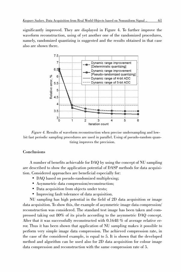
Kaspars Sudars. Data Acquisition from Real World Objects based on Nonuniform Signal ..
significantly improved. They are displayed in Figure 4. To further improve the waveform reconstruction, using of yet another one of the randomized procedures, namely, randomized quantizing is suggested and the results obtained in that case also are shown there.
Figure 4. Results of waveform reconstruction when precise undersampling and low-bit fast periodic sampling procedures are used in parallel. Using of pseudo-random quan-
tizing improves the precision.
Conclusions
A number of benefits achievable for DAQ by using the concept of NU sampling are described to show the application potential of DASP methods for data acquisi-tion. Considered approaches are beneficial especially for:
• DAQ based on pseudo-randomized multiplexing;• Asymmetric data compression/reconstruction;• Data acquisition from objects under tests;• Improving fault tolerance of data acquisition.
NU sampling has high potential in the field of 2D data acquisition or image data acquisition. To show this, the example of asymmetric image data compression/reconstruction was considered. The standard test image has been taken and com-pressed taking out 80% of its pixels according to the asymmetric DAQ concept. After that it was successfully reconstructed with 0.1648 % of average relative er-ror. Thus it has been shown that application of NU sampling makes it possible to perform very simple image data compression. The achieved compression rate, in the case of the considered example, is equal to 5. It is shown that the developed method and algorithm can be used also for 2D data acquisition for colour image data compression and reconstruction with the same compression rate of 5.
61
LURaksti787-datorzinatne.indd 61LURaksti787-datorzinatne.indd 61 23.10.2012 12:02:3223.10.2012 12:02:32

5. Methods for Data Acquisition Exploiting Advantages of Pseudo-randomized Quantizing
Specifics of DAQ based on pseudo-randomized quantizing (PRQ) are consid-ered in more detail in the particular case of impedance measurement data acquisi-tion and pre-processing. Impact of signal quantizing on DAQ resolution and DFT coefficient estimation precision is considered and the potential of pseudo-random-ized quantizing for resolution improvement is shown.
The impedance (including bioimpedance) measurements in many cases could be reduced to estimation of the signal spectra on specific pre-determined frequen-cies. The task of this spectrum analysis is made more difficult by the fact that the frequency range of interest is wide. While effective methods and techniques for impedance measurements at frequencies up to several MHz have been developed and are used, there are problems when the spectrum analysis of the modulated im-pedance signals has to be performed in the frequency range up to several hundreds of MHz or even up to several GHz. The involved data acquisition and processing tasks then become rather challenging. In particular, data have to be processed in real-time and with sufficiently high resolution.
Processing of impedance signals on the basis of complexity reduced DFT
The pseudo-randomly quantized signal values contain significantly increased number of bits in comparison with deterministically or randomly quantized signals as the value of the pseudo-random noise �k , used at quantizing, is added [15, 16]. Di-rectly processing of the quantized signal clearly leads to a complicated processing pro-cedure. The problem was considered and it is shown how to avoid these complications. Suppose impedance signal demodulation is on estimation of the Fourier coefficients.
It is suggested to do that on the basis of the following equations:
1 1
1 1
2 2ˆ ˆ cos2 cos2
2 2ˆ ˆ sin 2 sin 2
N Na
i k i k k i k ik kN N
bi k i k k i k i
k k
qa x f t n f tN N
qb x f t n f tN N
(6)
Where ai and b
i are corrections:
1
1
2 1( )cos22
2 1( )sin 22
Nai k i k
kN
bi k i k
k
q f tNq f t
N
(7)
These corrections remain constant, can be pre-calculated for all excitation fre-quencies and used. The advantage of this approach to estimation of the Fourier coef-ficients is evident. Data can be processed in this case in a very simple and fast way.
62 COMPUTER SCIENCE AND INFORMATION TECHNOLOGIES
LURaksti787-datorzinatne.indd 62LURaksti787-datorzinatne.indd 62 23.10.2012 12:02:3223.10.2012 12:02:32

Kaspars Sudars. Data Acquisition from Real World Objects based on Nonuniform Signal ..
Obtained results of the suggested method
Diagrams given in Figure 5 illustrate the precision obtainable at using the suggest-ed methods for impedance data acquisition and demodulation of the impedance signals.
Figure 5. Estimates of the demodulated signal obtained by using deterministic quan-tizing (1) and pseudo-randomized quantizing (2). Averaged estimates based on the com-plexity-reduced approach using sign(sin) and sign(cos) functions are given as curve (3).
Demodulation quality improvement by fi ltering
After impedance signal demodulation, the extra precision of processing could be obtained with ordinary digital filtering. For this purpose application of the mov-ing average filter MAF is considered. If it is needed such filtering could be used iteratively. Also it is expected that usage of other filter types, like low-pass filters LPF, would provide good results.
Figures in Table 1 illustrate comparison of signal quantization errors with and without filtering. As can be seen, the filtering in general reduces quantizing errors, no matter whether it is MAF or LPF filtering.
Table 1Typical relative quantizing error readings.
Moving average filter MAF length 3 5 7 91 Deterministic 4 bit quantizing (no filtering) 0.1010 0.1010 0.1010 0.10102 Deterministic 12 bit quantizing (no filtering) 0.00037 0.00037 0.00037 0.000373 4+4 bit PRQ quantizing (no filtering) 0.0994 0.0993 0.1005 0.10044 4+4 bit PRQ quantizing, LPF 0.0431 0.0403 0.0426 0.04065 Deterministic 4 bit quantizing, LPF 0.0642 0.0642 0.0642 0.06426 4+4 bit PRQ quantizing, MAF 0.0399 0.0294 0.0274 0.0271
63
LURaksti787-datorzinatne.indd 63LURaksti787-datorzinatne.indd 63 23.10.2012 12:02:3223.10.2012 12:02:32

As it can be seen the PRQ quantizing provides significantly better demodu-lated signal precision than the traditional deterministic quantizing.
Conclusions
Application specifics of the basic three signal quantizing methods (methods for deterministic, randomized and pseudo-randomized quantizing) for data acquisition are studied. In many cases PRQ proves to be the best of them. That, of course, depends on the particular application.
DFT is often needed for biomedical DAQ applications, where performance of bioimpedance signal demodulation is required. Methods for such signal processing are essential for design of medical equipment. This work considers impedance sig-nal demodulation based on calculations of DFT coefficients on several frequencies and the advantages of using PRQ are shown.
Due to these features, PRQ is an approach to quantizing that is rather valu-able for achieving high performance of DAQ systems. That is confirmed by results obtained in the area of DAQ used for impedance data acquisition.
It is shown that in this application area:• Improved resolution of very fast low bit rate ADCs (several GHz sampling
frequency) at wideband low bit rate DAQ. In other words, PRQ reduces the quantizing bit rate, widening the application range of rough quantizing;
• Better digitized signal quality (in terms of signal sample values precision);• Simplified, energy efficient DAQ hardware and impedance signal process-
ing.In general, the obtained research results confirm that design and performance
of DAQ systems often can be significantly improved by exploiting PRQ.
5. Data Acquisition Based on Gathering Timing Information
The specific approach to signal sampling, based on detection of signal and reference function crossings is considered further. It is shown that under certain conditions it is possible to represent analog signals with timed sequences of events without loss of information and that this possibility can be exploited for develop-ing competitive DAQ systems based on detection of signal and reference crossing events (SRC sampling) that have attractive and useful advantages.
The comprehensive comparison of the classical signal sampling method and suggested method for SRC sampling is given in Table 2.
64 COMPUTER SCIENCE AND INFORMATION TECHNOLOGIES
LURaksti787-datorzinatne.indd 64LURaksti787-datorzinatne.indd 64 23.10.2012 12:02:3223.10.2012 12:02:32

Kaspars Sudars. Data Acquisition from Real World Objects based on Nonuniform Signal ..
Table 2Comparison of two alternative sampling approaches.
Classical sampling approach SRC sampling approachSignal sample value acquiring
• Signal sample values are taken at predetermined time instants
• Sample values are represented by respective voltage (current) levels
• Uniformly spaced signal sample values• Remote sampling implementations
usually not acceptable• Aliasing determined by Nyquist
frequency
• Sample values are taken at the signal and reference function crossing instants
• Sample values are represented by the time instants when the crossing events take place
• Nonuniformly spaced signal sample values• Remote sampling applicable• Specific aliasing conditions• Reference function defines the envelope of
the sampled signal instantaneous values Signal sample value transmission
• Requires transmission of constant levels• Sensitive to the ambient noise• Transmission acceptable only over short
distances
• Based on transmission of time instants• Relatively insensitive to the ambient noise• Transmission might be performed over
relatively large distances• Provides for data compression
Quantizing
• Sample values are quantized directly • Reference function values are quantized at the crossing time instants
• High precision synchronization is requiredMulti-channel operation
• Based on switching the analog input signals
• Number of channels limited by hierarchic multiplexer structures
• No switching of analog signal performed• Multiplexing of channels, provided by
enabling function, is much simpler• Well suited to data acquisition from a large
quantity of signal sources• Well suited to the specifics of Ultra
Wideband communicationProcessing
• Based on the classical DSP algorithms • Typically specific algorithms are needed for processing
• Applicability of standard algorithms achievable under certain condition
• Complexity-reduced pre-processing Advantages for DAQ systems
• Features and obtainable benefits are well known
• Reduced complexity and power consumption at the DAQ system front-end part
• Significantly enlarged number of data channels
65
LURaksti787-datorzinatne.indd 65LURaksti787-datorzinatne.indd 65 23.10.2012 12:02:3223.10.2012 12:02:32
Preference is given to the method for DAQ based on detection of signal and sine-wave crossing time instants, so-called SWC signal sampling method. The sine-wave is preferred as a reference function due to its positive characteristics, in particular, spectral purity of it. This significant feature of SWC sampling might be exploited for reducing the complexity of the algorithms for pre-processing of signals.
Potential of SWC sampling for simplifying some DSP algorithms
Algorithms for processing digital signals obtained in result of SWC sampling often can be significantly less complicated than the widely used conventional ones. In particular, in many cases it is possible to avoid multiplications of multi-bit num-bers. The unique constant envelope feature of SWC sampling makes it possible to develop rational algorithms, in particular, for Discrete Fourier Transform based spectrum analysis and waveform reconstruction. For example, the following equa-
tions can be used for calculation of Fourier coefficient estimates ia , ib not requir-ing multiplication of multi-digit numbers as usual [1, 2, 6]:
1
01
0
ˆ (sin 2 ( ) sin 2 ( ) )
ˆ (cos2 ( ) cos2 ( ) )
Nr
i r i k r i kkN
ri r i k r i k
k
Aa f f t f f tNAb f f t f f tN
(8)
Where Ar, fr are the amplitude and frequency of the sinusoidal reference func-tion, tk denotes the crossing time instants and N is the number of signal samples processed.
This approach to complexity reduction of algorithms for data pre-processing is usable only under the condition that the reference function is sinusoidal. This represents a strong argument in favour of using this type of reference functions. The problem related to the necessity of operating with sine and cosine functions in this case can be easily resolved by using look-up tables. The developed method for complexity-reduced digital filtering and parameter estimation is considered as an invention and the respective European patent application is published [6].
SWC sampled signal properties in the frequency domain
SWC sampled signal properties in the frequency domain are quite specific and they were explored in detail. First of all, SWC represents a specific modification of NU sampling and, as it is typical for this type of sampling, SWC has anti-aliasing properties. It is shown that there is no full-scale frequency overlapping. While peaks appear in the spectrogram at some indicated and defined frequencies, they are significantly suppressed. This type of aliasing is considered as so-called fuzzy aliasing [15].
66 COMPUTER SCIENCE AND INFORMATION TECHNOLOGIES
LURaksti787-datorzinatne.indd 66LURaksti787-datorzinatne.indd 66 23.10.2012 12:02:3223.10.2012 12:02:32

Kaspars Sudars. Data Acquisition from Real World Objects based on Nonuniform Signal ..
Data acquisition based on SWC sampling
Data acquisition based on SWC sampling is illustrated in Figure 6. Digitally timed events, defined as crossings of an input signal and a reference function, is used in this case for representation of analog signals in the digital domain. The most responsible elements of this system apparently are the comparators used for detection of the time instants tk at which the signal x(t) intersects the reference function r(t) that is given as a sine wave at frequency fr. It has constant amplitude Ar. The physical output y(t) of the comparator is formed as a pulse whenever the sampler is enabled by a function z(t) (Figure 6(b)) and a crossing of the input signal x(t) and the reference function r(t) takes place.
Figure 6. Time diagrams illustrating specific two types of input signal representation in the digital domain. (a) sampling based on signal and the reference function crossings; (b) enabling function; (c) analog carrier of information; (d) digital carrier of information.
These pulses y(t) at the sampler output are formed so that they carry the timing information indicating the exact crossing instants tk of the signal and the reference function. It is assumed that the output pulses, having sharp front edges are formed with a constant delay after each signal and the reference sine-wave crossings. Thus the sampler output signal is carrying the original information encoded as the se-quence {tk} of the sine-wave crossing instants. It is transferred over some shorter or longer distance to the host computer. Note that this sequence fully represents the respective input signal. It means that the crossing instant sequence might be
67
LURaksti787-datorzinatne.indd 67LURaksti787-datorzinatne.indd 67 23.10.2012 12:02:3223.10.2012 12:02:32

used either for recovery of the input signal sample values and reconstruction of the signal or the input data processing might be based on direct processing of these crossing instants as it is explained below [8]. While the sequence of the signal and reference function crossing instants represents in this case the input analog signal in the digital domain, either an analog or a digital carrier may be used for trans-mitting this information. A train of position-modulated short pulses (Figure 6(c)) is used as an analog information carrier and a sequence of digital crossing instant values {tk} (Figure 6(d)).
The analog carrier is used primarily for gathering and transmission of data from the cluster of remote samplers to the master part of the distributed ADC (Figure 7). The digital carrier is used at the stages of data reconstruction and/or their pre-processing and data transfer to computers.
While various techniques might be used for the recovery of the input signal sample values, basically a replica of the reference function waveform is sampled and quantized for that. Note that this copy of the reference function could be given either in analog or digital format. The signal sample values, of course, might be recovered and presented digitally in both cases.
Architecture of an energy-effi cient system for multichannel data acquisition
The suggested hardware architecture for simultaneous multichannel data ac-quisition is shown in Figure 7. Reduction of power consumption to a large extent is due to the method used for sampling. Application of it not only leads to the simplicity of the front-end design of this system. Remote samplers that can be placed directly at the locations of the sensors then are used rather than ADCs. This approach is well suited for remote signal sampling applications and for building the shown architecture of the system that actually is a distributed ADC. As can be seen, the sampling and quantising operations, in this structure, are distanced. This approach makes it possible to use many remote samplers at the front-end of it and to gather data from them in a rational way. To ensure proper performance of them in parallel, specific enabling control functions are introduced and used. Only those crossings are taken into account that happen during the time intervals when the respective comparator is enabled by a specially generated enabling function. This enabling function is exploited also for executing the input multiplexing. The analog input signal switching could be avoided then and that certainly is a significant positive fact.
At the current technological level, if the SWC based DAQ is implemented on available ICs, this limit is approximately 25 MHz for 8 to 10 bit quantizing. It is not so easy to achieve it. More realistic figures are 5–10 MHz with the quantization rate up to 12 bits. This result was obtained testing the experimental system developed in the framework of ERAF project Nr. VDP1/ERAF/CFLA/05/APK/2.5.1/000024/012 “Development of multi-channel systems for acquisitions of data from biomedical,
68 COMPUTER SCIENCE AND INFORMATION TECHNOLOGIES
LURaksti787-datorzinatne.indd 68LURaksti787-datorzinatne.indd 68 23.10.2012 12:02:3223.10.2012 12:02:32

Kaspars Sudars. Data Acquisition from Real World Objects based on Nonuniform Signal ..
ecological and industrial systems and transferring them to computerized systems”, co-sponsored by the European Union. This leads to the maximal number of chan-nels equal to 1000 for the mean sampling frequency equal to 20 KHz. Then the input signal could be processed in the alias-free way within the bandwidth 0–10 KHz. More often than not the required input numbers are smaller. Then the input signal bandwidth could be proportionally widened. To achieve results fully reflect-ing the potential of this approach, special ASICs for the analog-digital front end devices must be developed and used.
Figure 7. Architecture of the considered energy-efficient system fulfilling simultane-ous data acquisition functions based on SWC sampling.
Achieving the applicability of standard DSP algorithms
To avoid SWC sampling nonuniformities, regularization of SWC sampling results is considered. The very simple method for this regularization has been developed and is suggested. It has remarkable advantages in comparison with other reconstruction methods where burdensome signal processing is involved. The suggested signal regularization does not require any additional computation power at all. Of course, the results may be acceptable for end-users only under certain conditions.
69
LURaksti787-datorzinatne.indd 69LURaksti787-datorzinatne.indd 69 23.10.2012 12:02:3223.10.2012 12:02:32

Regularization of SWC sampling leads to obtain the possibility of using standard DSP algorithms for processing SWC sampled signals. Whenever this type of regularization is carried out, the wealth of existing DSP algorithms can be used for processing the signal sample values obtained in result of SWC sampling. This method can be implemented with help of the enabling function.
The curves in Figure 8 have been obtained varying signal sampling frequency and keeping constant reference frequency. The reference frequency, with the
enabling decimation factor n varying, was changed according to s rf f n . Then with n growing, the sampling conditions are becoming closer to regular until it reaches the point at which the sampling mode could be considered as regular and all DSP algorithms can be directly applicable. Unfortunately the regularization process proportionally decreases the signal sampling frequency.
Figure 8. Signal-to-noise ratio SNR versus decimation coefficient n of the activated reference function periods for three various signals.
How it can be seen from Figure 8, the SNR is acceptable starting to 20-th acti-vated sine-wave half period. Actually it depends on particular application.
Conclusion
Studies of SWC based DAQ lead to the following conclusions:• Algorithms and signal processing. Signals sampled according to the SWC
method has constant envelope not depending on the original analog signal frequency content. That makes it possible to develop algorithms for pro-cessing them without massive multiplication of multi-digit numbers.
• A new signal filtering algorithms, exploiting the constant envelope prop-erty, have been developed is described in [6].
• DFT without massive multiplication operation is possible.
70 COMPUTER SCIENCE AND INFORMATION TECHNOLOGIES
LURaksti787-datorzinatne.indd 70LURaksti787-datorzinatne.indd 70 23.10.2012 12:02:3323.10.2012 12:02:33
Kaspars Sudars. Data Acquisition from Real World Objects based on Nonuniform Signal ..
• Applicability of traditional DSP algorithms under certain conditions has been achieved. This applicability of classical DSP algorithms can be ob-tained by using regularization process of SWC sampled signals.
• To gain from of the constant envelope sampling, it has to be learned how to effectively cope with the drawbacks related to the nonuniformity of the obtained digital signals. The signal regularization using the enabling func-tion is recommended as effective tools for controlling signal sampling con-ditions. However it reduces the mean signal sampling rate for each DAS channel depending on particular application.
• Sampling properties. The SWC sampling properties are evaluated in the time domain and as well as in the frequency domain. Trading-off the mean sampling rate against the time resolution has to be done to provide for proper quality sampling. It is considered how the particularities of this type of signal spectra differ from spectra of the traditionally sampled signals.
• DAQ system architecture. Application of SWC sampling leads to simpler and more energy efficient hardware architectures of data acquisition sys-tems as the signal sampling operation can be performed on the basis of a single comparator instead of ADC.
The main conclusion is that SWC signal sampling method is well suited to simultaneous multi-channel data acquisition from a large number of relatively low-frequency signal sources.
6. FPGA based implementation of the considered DAQ methods
A particular application of DASP theory for Fourier coefficient calculation has been considered. FPGA based implementation of a specific DFT multiplier-less structure (F-DFT Processor) for fast pre-processing of data has been developed and FPGA implementation specifics studied. This type of FPGA is applicable for de-signs of various application-specific systems fulfilling digital signal pre-processing related to data time-frequency representation, data compression/reconstruction, spectrum analysis, filtering, parameter estimation and demodulation.
Experimental system has been programmed and tested on the basis of Altera Cyclone II EP2C70F672C6N chip model. The core of F-DFT Processor is multi-plier-less Adder-Subtractor Matrix. In addition to this Matrix, there are data input and output subsystems. Designs of these subsystems depend on specifics and re-quirements of various applications. Therefore the data input and output version is just one of the possible modifications. Real-time DFT and batch processing of data for DFT are two of the most often needed types of data pre-processing that can be performed on the basis of the developed FPGA chip.
71
LURaksti787-datorzinatne.indd 71LURaksti787-datorzinatne.indd 71 23.10.2012 12:02:3323.10.2012 12:02:33

Requirements dictated by a specific bioimpedance measurement system were taken into account at definition of the parameters of DFT for the specification of this FPGA chip. These parameters are the following: Fourier coefficients have to be calculated simultaneously at frequencies f0 (data mean value), f1, f2, f4, f8, f16, f32 and f64 by processing N=256 real signal sample values. The absolute values of these frequencies depend only on the parameters of data acquisition, in particu-lar, on the specifics of the signal source and the used ADC. Thus the considered processor can perform DFT in a wide frequency range from KHz up to GHz.
The most important parameter that has to be experimentally measured is the achieved pin-to-pin delays characterizing the Matrix, as this parameter actually defines the upper repetition rate of DFT operation or system clock frequency. Print-out of so-called Clock setup, showing pin-to-pin delays for the involved data flows at the specified frequencies, follows.
Figure 9. Printout showing test results of the F-DFT Processor measured by Quartus soft-ware. Achievable clock frequencies for various data flow routes and the related pin-to-pin
delays are given for the indicated addresses.
As can be seen in Figure 9, the worst case is for the data flow in the Matrix from register reg[231][7] to the output f8c7[0]. According to Figure 9, the achievable clock frequency of the F-DFT processor under the described conditions is 101.49 MHz and the worst-case pin-to-pin delay is 9.853 ns. Required resources for the F-DFT processor design are given in the printout of Figure 10.
72 COMPUTER SCIENCE AND INFORMATION TECHNOLOGIES
LURaksti787-datorzinatne.indd 72LURaksti787-datorzinatne.indd 72 23.10.2012 12:02:3323.10.2012 12:02:33

Kaspars Sudars. Data Acquisition from Real World Objects based on Nonuniform Signal ..
Figure 10. Required resources of the designed F-DFT processor (Altera Quartus snapshot).
In comparison with the classical structure of the digital FIR filter on 256 coef-ficients design of the F-DFT processor requires much less elements, approximately 2 times less Altera logical elements. Performance of both devices is character-ized by pin-to-pin delays and the clock frequency. To compare both, the following points have to be taken into account: (1) the considered particular F-DFT processor calculates simultaneously outputs of 15 filters (1 filter for f0 and two filters for each other 7 frequencies) in parallel; (2) the structure of the considered single FIR filter is pipelined, therefore the indicated clock frequency for it depends on the delay of only a single filter stage.
For the explained reasons, the performance of both devices cannot be directly compared. As to the resources, the requirements of F-DFT are significantly reduced.
Table 3Summary of required resources and parameters of the F-DFT processor and
a particular digital FIR fi lter.
Cyclone II Device EP2C70F672C6
F-DFT data block 256
Pipelined FIR on 256 coeffi cients with
256 multipliersClock frequency 101.49 MHz 117.25 MHzTotal combinational functions 11,640 / 68,416 ( 17 % ) 28,785 / 68,416 ( 42 % )Dedicated logic registers 7,498 / 68,416 ( 11 % ) 16,807 / 68,416 ( 25 % )Total logic elements 14,108 / 68,416 ( 21 % ) 29,115 / 68,416 ( 43 % )Total pins 26 / 422 ( 7 % ) 30 / 422 ( 7 % )Embedded Multiplier 9-bit
elements0 / 300 ( 0 % ) 0 / 300 ( 0 % )
73
LURaksti787-datorzinatne.indd 73LURaksti787-datorzinatne.indd 73 23.10.2012 12:02:3323.10.2012 12:02:33
7. Obtained research results
Overview of the specifics related to development and production of currently available DAQ systems reveals the basic tendencies characterizing the situation in this field. While about 300 industrial companies are active in this area and seem-ingly many various DAQ systems are offered, actually progress there is relatively slow. As it is shown the basic limiting factor is the dependency of DAQ methods on the classical theory of DSP, especially on the dominating theoretical principles of periodic sampling. Theory of randomized and alias-free signal processing is rather well suited for DAQ applications. This fact has been taken into account and the undertaken research activities of these doctoral studies are based on and exploit a number of essential results of the DASP theory. The point is that signal digitizing performed in this way is rather flexible and can be adjusted to the needs of various DAQ applications. The approach to DAQ is based on these considerations.
Summary of the obtained research results follows:1. Research results related to exploitation of nonuniform sampling for DAQ
showing that this approach has significant potential for improving DAQ. The obtained results in this area, specifically, are the following:
• Elimination of the input signal source number dependence on the sampling rate that limits the capabilities of the classical DAQ sys-tems. That makes possible simultaneous data acquisition in paral-lel from a significantly increased (up to 8-12 times) number of signal sources.
• Development of methods and algorithms for asymmetric data com-pression/reconstruction (in the sense that most of the computation-al burden is put on the reconstruction stage), including very fast image data asymmetric compression/reconstruction.
• Development, making and testing of an experimental complexity-reduced hardware/software system for image data compression based on this method, achieving image data compression up to 5 times for various images, including colour and standard images.
• Development, analysis and description of various approaches to DFT coefficient estimation, in particular, for spectrum analysis of bioimpedance data obtained in result of nonuniform sampling based bioimpedance demodulation.
2. Obtained research results, related to exploitation of deterministic, ran-domized and pseudo-randomized quantizing methods for DAQ, are the following:
• Results of analysis and evaluation of the impact pseudo-random-ized quantizing has on the precision of spectrum analysis of data.
• Methods for spectrum analysis of data, based on pseudo-random-ized signal quantizing.
74 COMPUTER SCIENCE AND INFORMATION TECHNOLOGIES
LURaksti787-datorzinatne.indd 74LURaksti787-datorzinatne.indd 74 23.10.2012 12:02:3323.10.2012 12:02:33

Kaspars Sudars. Data Acquisition from Real World Objects based on Nonuniform Signal ..
• Complexity reduced approach to bioimpedance data demodulation using DFT on the basis of rectangular functions.
• Results of comparison and evaluation of all three quantizing ver-sions showing that pseudo-randomized quantizing usually outper-forms two other quantizing options.
3. Results of research related to a new approach to DAQ based on acquiring timing information:
• A method for DAQ, based on detection of signal and sine-wave crossing instants (SWC sampling), computer-simulated and exten-sively explored.
• Computer simulation results showing the most significant advan-tage of SWC based DAQ systems, namely, their capability of data gathering from a very large quantity of signal sources (up to 256-512) distributed over an object of technical or biomedical origin.
• Method for SWC sampled signal regularization that can be per-formed to ensure the applicability of standard DSP algorithms.
• Special signal processing methods applicable in the case of SWC for complexity-reduced design of digital filters and multiplier-less structures for DFT [6].
4. Developed MATLAB programs for Computer simulations of the explored DAQ methods.
5. Results obtained in the experimental research area: VHDL description for FPGA implementation of a specific Fast DFT Processor, test results of this FPGA, showing, specifically, the required element count and param-eters characterizing the achieved operational speed.
8. Conclusions
The goal of this work, discovering innovative methods for efficient massive data acquisition from real life objects and supplying computers with this informa-tion, has been reached and the planned tasks have been fulfilled. The developed and investigated innovative methods for complexity-reduced DAQ and energy-effi-cient pre-processing of the data are based on the theory, concepts and methods of the non-traditional digital signal processing DASP. The obtained research results show: (1) how that can be done and (2) what can be gained at computer system linking to the real world technical and biological objects by using the developed DAQ methods.
The basic benefits that can be obtained in this way, specifically, are the fol-lowing:
1. The developed methods for multi-channel data acquisition systems are flexible and applicable for simultaneous data acquisition from many sig-nal sources.
75
LURaksti787-datorzinatne.indd 75LURaksti787-datorzinatne.indd 75 23.10.2012 12:02:3323.10.2012 12:02:33

2. Simultaneous data acquisition from many signal sources is performed in parallel under conditions where the upper frequencies of the input signal spectra do not depend on the quantity of the input channels.
3. Input signals can be sampled directly at their sources by front-end de-vices that are much simpler than the traditionally used ADCs.
4. Consequently, the power consumption of these front-end devices might be significantly lower.
However DASP technology is specific. Therefore hardware and software imple-menting DAQ based on this technology are specific as well. MATLAB based soft-ware tools have been developed and they could be used to implement the chosen approach. Streams of digitally timed sampling events are used as digital signals representing the acquired data. Massive data acquisition is based on pseudo-ran-domised time-sharing, analog-to-event and time-to-digital conversions.
Experimental investigations of the developed DAQ methods were carried out by using hardware tools that have been developed in the Laboratory 2.2.of Institute of Electronics and Computer Science in the framework of ERAF Project Nr. VDP1/ERAF/CFLA/05/APK/2.5.1/000024/012 “Development of multi-channel systems for acquisitions of data from biomedical, ecological and industrial systems and transferring them to computerized systems”, co-sponsored by the European Union. Author of this research work participated in this project as a member of the team.
Tests and experimental evaluation of the developed DAQ systems show that:1. Experiments confirm the results obtained theoretically. 2. The existing microelectronic components, including FPGA chips and
their programming technology, basically are suitable and can be used for implementation of gathered data specific pre-processing.
3. Potential of FPGA usage for specific data pre-processing is demonstrat-ed by performance of the developed Fast DFT Processor (see Protocol of F-DFT Processor international evaluation results given in Attachment).
4. Attempts to use the existing microelectronic components for implementa-tion of the front-end operations at DAQ show that this approach basically does not lead to sufficiently high results.
5. To fully gain from the research results obtained in the framework of this work, implementation of the front-end DAQ procedures, defined by the developed DAQ methods, should be based on developed new specific ASICs (Application Specific Integrated Circuits).
References
1. Bilinskis I., Sudars K. Processing of signals sampled at sine-wave crossing instants. Proceedings of the “2007 Workshop on Digital Alias-free Signal Processing” (WDASP’07), London, UK, 17 April 2007, pp. 45-50.
2. Sudars K., Ziemelis Z., Expected performance of the sine-wave crossing data acquisition systems, Proceedings of DASP Workshop, London, UK, 17 April 2007.
76 COMPUTER SCIENCE AND INFORMATION TECHNOLOGIES
LURaksti787-datorzinatne.indd 76LURaksti787-datorzinatne.indd 76 23.10.2012 12:02:3323.10.2012 12:02:33

Kaspars Sudars. Data Acquisition from Real World Objects based on Nonuniform Signal ..
3. Bilinskis I., Sudars K. Digital representation of analog signals by timed sequences of events, “Electronics and Electrical Engineering”, No. 3(83), March, 2008, Presented in International Conference “Electronics 2008”, Kauna, Lithuania, 20-22 May 2008.
4. Bilinskis I., Sudars K. Specifics of constant envelope digital signals, “Electronics and Electrical Engineering”, No. 4(84), April, 2008, Presented in International Conference “Electronics 2008”, Kauna, Lithuania, 20-22 May 2008.
5. Artyukh Yu., Bilinskis I., Sudars K., Vedin V., Multi-channel data acquisition from sensor systems. Proceedings of the 10th International Conference “Digital Signal Processing and its Applications” (DSPA’2008), Moscow, Russia, 2008, Vol.X-1, pp.117-119.
6. Artyukh Y., Bilinskis I., Sudars K., European Patent Application No. EP2075912 A1, Method for complexity-reduced digital filtering and parameter estimation of analog signals, Assignee: Institute of Electronics and Computer Science of Latvia, European patent Bulletin, January 7, 2009.
7. Bilinskis I., Sudars K., Min M., Annus P., Advantages and limitations of an approach to bio-impedance data acquisition and processing relying on fast low bit rate ADCs, Baltic Electronic Conference BEC 2010, Tallinn, Estonia, 4.-6. October 2010.
8. Artyukh Y., Bilinskis I., Roga S., Sudars K., Digital Representation of Analog Signals leading to their Energy-efficient Processing, Green Information Technology (GREEN IT 2010), Singapore, 25.-26. October 2010.
9. Sudars K., Data Acquisition Based on Nonuniform Sampling: Achievable Advantages and Involved Problems, “Automatic Control and Computer Science” Magazine, Allerton Press, 2010, Vol. 44, No. 4, pp. 199-207.
10. Bilinskis I., Skageris A., Sudars K. Method for fast and complexity-reduced asymmetric image compression, “Electronics and Electrical Engineering”, No. 4(110), May, 2011, Presented in International Conference “Electronics 2011”, Kauna, Lithuania, 17-19 May 2011.
11. Artyukh Y., Bilinskis I., Rybakov A., Sudars K., Vedin V., Modular Multi-channel Data Acquisition Systems, “Automatic Control and Computer Sciences” Magazine, Allerton Press, 2008, Vol. 42, No. 3, pp. 113–119.
12. Artyukh Y., Bilinskis I., Boole E., Rybakov A., Vedin V., “Wideband RF signal digititizing for high purity spectral analysis,” Proceedings of the 2005 International Workshop on Spectral Methods and Multirate Signal Processing, (SMMSP 2005) June 20-22, 2005, Riga, Latvia. pp. 123-128.
13. Artyukh Y., Bilinskis I., Greitans M., Mednieks I., Rybakov A., DASP-Lab System – a demonstra-tor of the new DSP technology. //Automatic Control and Computer Science, Allerton Press, 2000, No. 6, pp. 3-21.
14. Artyukh Y., Bilinskis I., Rybakov A., Stepin V., “Pseudo-randomization of multiplexer-based data acquisition from multiple signal sources,” Proceeding of DASP Workshop, London, UK, 17 April 2007.
15. Bilinskis I., Digital Alias-free Signal Processing, Wiley, 2007, ISBN: 978-0-470-02738-716. Bilinskis I., Mikelsons A., Randomized Signal Processing, Prentice Hall, 1992, ISBN: 0-13-
751074-817. Bilinskis I., Rybakov A., “Iterative spectrum analysis of nonuniformly undersampled wideband
signals,” Electronics and Electrical Engineering, 2006, vol. 4(68), pp. 5-8.18. Blackledge J. M., Burge R. E., Barratt N. R., “Phase imaging by real-zero conversion and its ap-
plications to synthetic aperture radar”, Journal of Physics D: Applied Physics, Volume 20, Issue 11, November 14, 1987
19. Borokhovych Y., Gustat H., “4-bit, 15 GS/s ADC in SiGe,” NORCHIP 2008, 16-17 Nov. 2008, Tallinn, Estonia, pp. 268-271.
20. Candès E. J., Wakin M. B., “An Introduction to Compressive Sampling”, IEEE Signals Processing Magazine, March 2008
21. Contadini F., “Oversampling with averaging to increase ADC resolution”, Internet: http://www.embedded.com/design/223000385, 1 March 2010 15
77
LURaksti787-datorzinatne.indd 77LURaksti787-datorzinatne.indd 77 23.10.2012 12:02:3323.10.2012 12:02:33

22. Daria V. R., Saloma C., “High-accuracy Fourier transform interferometry, without oversampling, with a 1-bit analog-to-digital converter”, Applied Optics, Volume 39, Issue 1, January 1, 2000, pp. 108-113
23. Eng F., Non-Uniform Sampling in Statistical Signal Processing, Dissertation at Linköpings Universitet, Sweden, 2007, ISBN: 978-91-85715-49-7
24. Internet: http://en.wikipedia.org/wiki/Data_acquisition 25. Internet:http://www.datatranslation.com/docs/whitepapers/benefits_simulataneous_daq.pdf 26. Internet: http://www.radiolocman.com/news/new.html?di=64921 27. Koch P., Prasad R., “The Universal Handset,” IEEE Spectrum, vol. 46, pp. 32-37, April 2009. 28. Kumaresan R., Wang Y., “On representing signals using only timing information”, The Journal of
the Acoustical Society of America, Volume 110, Issue 5, November 2001, pp. 2421-243929. Lim M., Saloma C., “Direct signal recovery from threshold crossings”, Physical Review E
(Statistical Physics, Plasmas, Fluids, and Related Interdisciplinary Topics), Volume 58, Issue 5, November 1998, pp. 6759-6765
30. Logan Jr. B. F., “Information in the zero crossings of bandpass signals”, Bell System Technical Journal, Volume 56, April 1977, pp. 487-510
31. Marvasti F. (editor), Nonuniform Sampling Theory and Practice, Kluwer Academic/Plenum Publishers, 2001, ISBN: 0-306-46445-4
32. Marvasti F., A Unified Approach to Zero-crossings and Nonuniform Samplingof single and mul-tidimensional signals and systems, Illinois Institute of Technology, 1987, ISBN: 0-9618167-0-8
33. Min M., Bilinskis I., Artyukh Y., Annus P., Land R., Märtens O., “Nonuniform Sampling and Demodulation for Wideband Multi-frequency Bioimpedance Measurements,” Proceedings of the Workshop on Digital Alias-free Signal Processing, London, 17 April 2007
34. Nait-Ali A., Cavaro-Menard C. (editors), Compression of Biomedical Images and Signals, Wiley, 2008, ISBN: 978-1-84821-028-8
35. Nazario M. A., Saloma C., “Signal recovery in sinusoid-crossing sampling by use of the mini-mum-negativity constrain”, Applied Optics, Volume 37, Issue 14, May 10, 1998
36. Papenfus F., Digital Signal Processing of Nonuniformly Sampled Signals, Dissertation at Universität Rostock, Publisher: Shaker Verlag, 2008, ISBN: 978-3-8322-6895-4
37. Raghavendra C. S., Sivalingam K. M., Znati T. (editors), Wireless Sensor Networks, Kluwer Academic, 2004, ISBN-13: 978-1402078835
38. Rieke F., Warland D., R. R. van Steveninck, Bialek W., “Spikes: Exploring the Neural Code”, MIT Press, Cambridge, MA, 1997
39. Sundstrom T., Alvandpour A., “A 2.5-GS/s 30-mW 4-bit Flash ADC in 90nm CMOS,” NORCHIP 2008, 16-17 Nov. 2008, Tallinn, Estonia, pp. 264-267.
40. Zeevi Y. Y., Gavriely A., Shamai (Shitz) S., “Image representing by zero and sine-wave cross-ings”, Journal of the Optical Society of America A, pp. 2045-2060, 1987
78 COMPUTER SCIENCE AND INFORMATION TECHNOLOGIES
LURaksti787-datorzinatne.indd 78LURaksti787-datorzinatne.indd 78 23.10.2012 12:02:3323.10.2012 12:02:33
12 12 12 12
1
2
SCIENTIFIC PAPERS, UNIVERSITY OF LATVIA, 2012. Vol. 787COMPUTER SCIENCE AND INFORMATION TECHNOLOGIES 79–105 P.
LURaksti787-datorzinatne.indd 79LURaksti787-datorzinatne.indd 79 23.10.2012 12:02:3323.10.2012 12:02:33

•
80 COMPUTER SCIENCE AND INFORMATION TECHNOLOGIES
LURaksti787-datorzinatne.indd 80LURaksti787-datorzinatne.indd 80 23.10.2012 12:02:3323.10.2012 12:02:33

Atis Elsts, Girts Strazdins, et al. Design and Implementation of MansOS: a Wireless ..
•
81
LURaksti787-datorzinatne.indd 81LURaksti787-datorzinatne.indd 81 23.10.2012 12:02:3323.10.2012 12:02:33

82 COMPUTER SCIENCE AND INFORMATION TECHNOLOGIES
LURaksti787-datorzinatne.indd 82LURaksti787-datorzinatne.indd 82 23.10.2012 12:02:3323.10.2012 12:02:33

Atis Elsts, Girts Strazdins, et al. Design and Implementation of MansOS: a Wireless ..
•
•
•
•
83
LURaksti787-datorzinatne.indd 83LURaksti787-datorzinatne.indd 83 23.10.2012 12:02:3323.10.2012 12:02:33

84 COMPUTER SCIENCE AND INFORMATION TECHNOLOGIES
LURaksti787-datorzinatne.indd 84LURaksti787-datorzinatne.indd 84 23.10.2012 12:02:3323.10.2012 12:02:33

Atis Elsts, Girts Strazdins, et al. Design and Implementation of MansOS: a Wireless ..
2
85
LURaksti787-datorzinatne.indd 85LURaksti787-datorzinatne.indd 85 23.10.2012 12:02:3323.10.2012 12:02:33

2
2
2
86 COMPUTER SCIENCE AND INFORMATION TECHNOLOGIES
LURaksti787-datorzinatne.indd 86LURaksti787-datorzinatne.indd 86 23.10.2012 12:02:3423.10.2012 12:02:34

Atis Elsts, Girts Strazdins, et al. Design and Implementation of MansOS: a Wireless ..
••
•
•
A BA B
87
LURaksti787-datorzinatne.indd 87LURaksti787-datorzinatne.indd 87 23.10.2012 12:02:3423.10.2012 12:02:34

••
88 COMPUTER SCIENCE AND INFORMATION TECHNOLOGIES
LURaksti787-datorzinatne.indd 88LURaksti787-datorzinatne.indd 88 23.10.2012 12:02:3423.10.2012 12:02:34
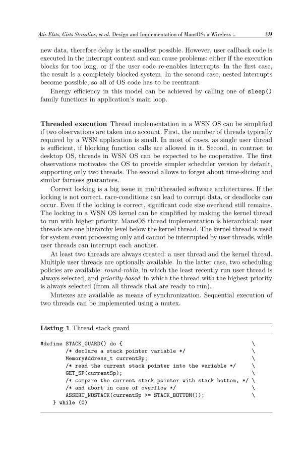
Atis Elsts, Girts Strazdins, et al. Design and Implementation of MansOS: a Wireless .. 89
LURaksti787-datorzinatne.indd 89LURaksti787-datorzinatne.indd 89 23.10.2012 12:02:3423.10.2012 12:02:34

90 COMPUTER SCIENCE AND INFORMATION TECHNOLOGIES
LURaksti787-datorzinatne.indd 90LURaksti787-datorzinatne.indd 90 23.10.2012 12:02:3423.10.2012 12:02:34

Atis Elsts, Girts Strazdins, et al. Design and Implementation of MansOS: a Wireless ..
Data CRC
Flash memory
Segment
Data block
Data chunk
10 10 01 10
01 01 01 01
00 01 00 00
10 00 10 01
. . .
01 Free block
10 Allocated block
00 Available after erase
One segment
91
LURaksti787-datorzinatne.indd 91LURaksti787-datorzinatne.indd 91 23.10.2012 12:02:3423.10.2012 12:02:34
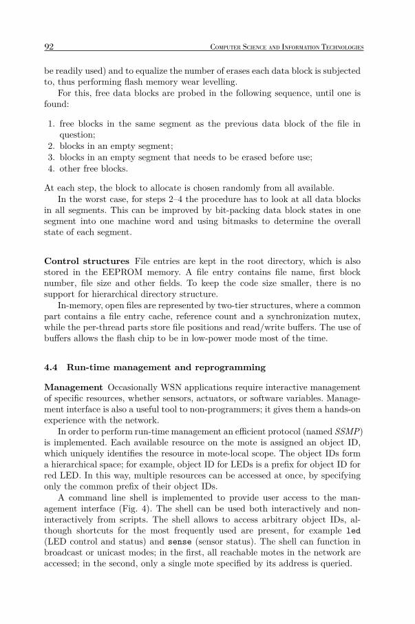
92 COMPUTER SCIENCE AND INFORMATION TECHNOLOGIES
LURaksti787-datorzinatne.indd 92LURaksti787-datorzinatne.indd 92 23.10.2012 12:02:3423.10.2012 12:02:34
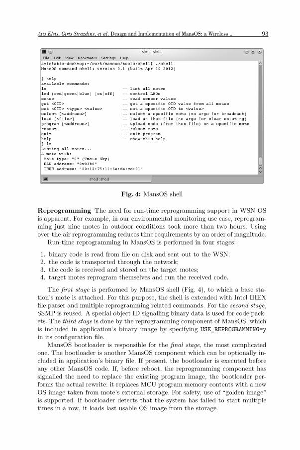
Atis Elsts, Girts Strazdins, et al. Design and Implementation of MansOS: a Wireless .. 93
LURaksti787-datorzinatne.indd 93LURaksti787-datorzinatne.indd 93 23.10.2012 12:02:3423.10.2012 12:02:34

2
94 COMPUTER SCIENCE AND INFORMATION TECHNOLOGIES
LURaksti787-datorzinatne.indd 94LURaksti787-datorzinatne.indd 94 23.10.2012 12:02:3423.10.2012 12:02:34

Atis Elsts, Girts Strazdins, et al. Design and Implementation of MansOS: a Wireless .. 95
LURaksti787-datorzinatne.indd 95LURaksti787-datorzinatne.indd 95 23.10.2012 12:02:3423.10.2012 12:02:34
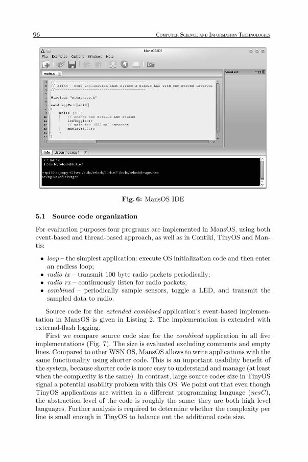
•
•••
96 COMPUTER SCIENCE AND INFORMATION TECHNOLOGIES
LURaksti787-datorzinatne.indd 96LURaksti787-datorzinatne.indd 96 23.10.2012 12:02:3423.10.2012 12:02:34

Atis Elsts, Girts Strazdins, et al. Design and Implementation of MansOS: a Wireless .. 97
LURaksti787-datorzinatne.indd 97LURaksti787-datorzinatne.indd 97 23.10.2012 12:02:3423.10.2012 12:02:34

98 COMPUTER SCIENCE AND INFORMATION TECHNOLOGIES
LURaksti787-datorzinatne.indd 98LURaksti787-datorzinatne.indd 98 23.10.2012 12:02:3423.10.2012 12:02:34

Atis Elsts, Girts Strazdins, et al. Design and Implementation of MansOS: a Wireless .. 99
LURaksti787-datorzinatne.indd 99LURaksti787-datorzinatne.indd 99 23.10.2012 12:02:3423.10.2012 12:02:34
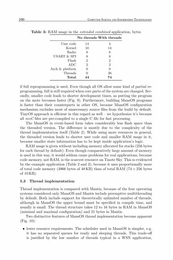
74 + 256
•
100 COMPUTER SCIENCE AND INFORMATION TECHNOLOGIES
LURaksti787-datorzinatne.indd 100LURaksti787-datorzinatne.indd 100 23.10.2012 12:02:3523.10.2012 12:02:35

Atis Elsts, Girts Strazdins, et al. Design and Implementation of MansOS: a Wireless ..
•
101
LURaksti787-datorzinatne.indd 101LURaksti787-datorzinatne.indd 101 23.10.2012 12:02:3523.10.2012 12:02:35
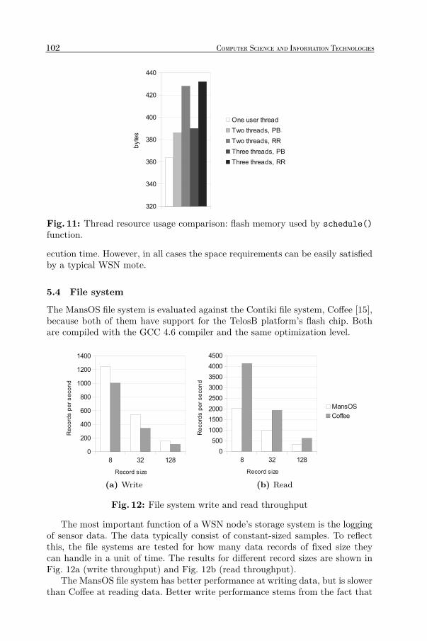
102 COMPUTER SCIENCE AND INFORMATION TECHNOLOGIES
LURaksti787-datorzinatne.indd 102LURaksti787-datorzinatne.indd 102 23.10.2012 12:02:3523.10.2012 12:02:35

Atis Elsts, Girts Strazdins, et al. Design and Implementation of MansOS: a Wireless ..
≈ 66
103
LURaksti787-datorzinatne.indd 103LURaksti787-datorzinatne.indd 103 23.10.2012 12:02:3523.10.2012 12:02:35

104 COMPUTER SCIENCE AND INFORMATION TECHNOLOGIES
LURaksti787-datorzinatne.indd 104LURaksti787-datorzinatne.indd 104 23.10.2012 12:02:3523.10.2012 12:02:35

Atis Elsts, Girts Strazdins, et al. Design and Implementation of MansOS: a Wireless .. 105
LURaksti787-datorzinatne.indd 105LURaksti787-datorzinatne.indd 105 23.10.2012 12:02:3523.10.2012 12:02:35

SCIENTIFIC PAPERS, UNIVERSITY OF LATVIA, 2012. Vol. 787COMPUTER SCIENCE AND INFORMATION TECHNOLOGIES 106–124 P.
LURaksti787-datorzinatne.indd 106LURaksti787-datorzinatne.indd 106 23.10.2012 12:02:3523.10.2012 12:02:35
Sergejs Kozlovics. Calculating The Layout For Dialog Windows Specified As Models
→ →
107
LURaksti787-datorzinatne.indd 107LURaksti787-datorzinatne.indd 107 23.10.2012 12:02:3623.10.2012 12:02:36
108 COMPUTER SCIENCE AND INFORMATION TECHNOLOGIES
LURaksti787-datorzinatne.indd 108LURaksti787-datorzinatne.indd 108 23.10.2012 12:02:3823.10.2012 12:02:38

Sergejs Kozlovics. Calculating The Layout For Dialog Windows Specified As Models
From Kernel Metamodel From Environment Metamodel
Componentenabled:Boolean=truereadOnly:Boolean=falsehint:String=""
horizontalSpan:Integer=1verticalSpan:Integer=1 minimumWidth:IntegerpreferredWidth:IntegermaximumWidth:IntegerminimumHeight:IntegerpreferredHeight:IntegermaximumHeight:Integer leftMargin:IntegerrightMargin:IntegertopMargin:IntegerbottomMargin:Integer onFocusGainedEvent:StringonFocusLostEvent:String
ContainerhorizontalAlignment:HorizontalAlignmentverticalAlignment:VerticalAlignmenthorizontalSpacing:IntegerverticalSpacing:IntegerleftBorder:IntegerrightBorder:IntegertopBorder:IntegerbottomBorder:IntegerleftPadding:IntegerrightPadding:IntegertopPadding:IntegerbottomPadding:Integer
Command
Event
Engine <<singleton>>DialogEngine
interfaceMetamodelVersion:String
RelativeInfoGroup RelativeInfo
<<enumeration>>HorizontalAlignmentLEFTCENTERRIGHT
<<enumeration>>VerticalAlignmentTOPCENTERBOTTOM
VerticalBox VerticalSplitBox
GroupBoxcaption:StringhasBorder:Boolean=true
Tabcaption:String
HorizontalBox HorizontalSplitBox
VerticalScrollBox
HorizontalScrollBox
VerticalScrollBoxWrapper
HorizontalScrollBoxWrapper
ScrollBox ScrollBoxWrapper
Column
Row
Stack
TabContainer
TabChangeEvent
Formcaption:StringclickEventOnClose:Boolean=truehasMinimizeButton=falsehasMaximizeButton=falseleft:Integertop:Integerwidth:Integerheight:IntegeronFormCloseEvent:String
ShowCommand
ShowModalCommand
CloseCommand
DeleteCommandButton
caption:StringcloseOnClick:BooleandeleteOnClick:BooleanonClickEvent:String
RefreshCommand
Labelcaption:String
CheckBoxcaption:Stringchecked:BooleanonChangeEvent:String
RadioButtoncaption:Stringselected:BooleanonClickEvent:String
InputFieldtext:StringonChangeEvent:String
MultiLineTextBoxonMultiLineTextBoxChangeEvent:String
TextLinetext:Stringinserted:Booleandeleted:Booleanedited:Boolean
Imagelocation:StringonChangeEvent:String
ComboBoxtext:Stringeditable:BooleanonChangeEvent:StringonDropDownEvent:String
ListBoxmultiSelect:BooleanonListBoxChangeEvent:StringonRightClickEvent:String
Itemvalue:String
MultiLineTextBoxChangeEvent
ChangeEvent
ListBoxChangeEvent
ClickEvent
FormCloseEvent
DropDownEvent
FocusGainedEvent
FocusLostEvent
RightClickEvent
Frameuri:Stringcaption:StringisResizeable:BooleanisClosable:Boolean
HorizontalRelativeInfominimumRelativeWidth:RealpreferredRelativeWidth:RealmaximumRelativeWidth:Real
VerticalRelativeInfominimumRelativeHeight:RealpreferredRelativeHeight:RealmaximumRelativeHeight:Real
DialogEngineCommand
DialogEngineEvent
* {ordered}0..1orderedFocusableComponent
*
next0..1
previous 0..1receiver 1source 1
*
10..1
10..1
component*activeTab 0..1
source
1
receiver1
receiver1
receiver1
receiver1
receiver1
defaultButton0..1cancelButton0..1
textLine*
0..1 currentLine0..1
*
*selectedItem
0..1
selectedItem*
inserted*deleted*edited* source 1
source0..1
source0..1
deselected*
selected*
source1
source0..1
source1 source1
source0..1
source0..1
source0..1
source0..1source0..1
source1
previousTab1
1
109
LURaksti787-datorzinatne.indd 109LURaksti787-datorzinatne.indd 109 23.10.2012 12:02:3923.10.2012 12:02:39

y
x
110 COMPUTER SCIENCE AND INFORMATION TECHNOLOGIES
LURaksti787-datorzinatne.indd 110LURaksti787-datorzinatne.indd 110 23.10.2012 12:02:3923.10.2012 12:02:39

Sergejs Kozlovics. Calculating The Layout For Dialog Windows Specified As Models 111
LURaksti787-datorzinatne.indd 111LURaksti787-datorzinatne.indd 111 23.10.2012 12:02:4123.10.2012 12:02:41

112 COMPUTER SCIENCE AND INFORMATION TECHNOLOGIES
LURaksti787-datorzinatne.indd 112LURaksti787-datorzinatne.indd 112 23.10.2012 12:02:4223.10.2012 12:02:42

Sergejs Kozlovics. Calculating The Layout For Dialog Windows Specified As Models 113
LURaksti787-datorzinatne.indd 113LURaksti787-datorzinatne.indd 113 23.10.2012 12:02:4323.10.2012 12:02:43
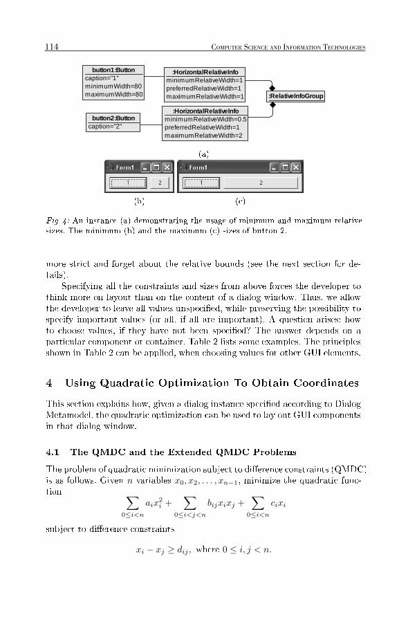
button1:Buttoncaption="1"minimumWidth=80maximumWidth=80
button2:Buttoncaption="2"
:HorizontalRelativeInfominimumRelativeWidth=1preferredRelativeWidth=1maximumRelativeWidth=1
:HorizontalRelativeInfominimumRelativeWidth=0.5preferredRelativeWidth=1maximumRelativeWidth=2
:RelativeInfoGroup
n x0, x2, . . . , xn−1
∑0≤i<n
aix2i +
∑0≤i<j<n
bijxixj +∑
0≤i<n
cixi
xi − xj ≥ dij , 0 ≤ i, j < n.
114 COMPUTER SCIENCE AND INFORMATION TECHNOLOGIES
LURaksti787-datorzinatne.indd 114LURaksti787-datorzinatne.indd 114 23.10.2012 12:02:4523.10.2012 12:02:45

Sergejs Kozlovics. Calculating The Layout For Dialog Windows Specified As Models
c1
c2
c3 c4∞
c5
∞
c6
c7c8
∞
c9c10 c11
c12 c13c14 c15 c16
c17
ci
∞∞
115
LURaksti787-datorzinatne.indd 115LURaksti787-datorzinatne.indd 115 23.10.2012 12:02:4623.10.2012 12:02:46

xi − xj ≥ dij ≥ mij ,
dijmij
dij dijdij ≥ mij dij
dij −mij
CxCL xC
R
yCT yCBxCLM xC
RM yCTM yCBM C CxCLB xC
RB yCTB yCBB
C xCLP xC
RP yCTP yCBP
x y
xCR − xC
L ≥ ;
xCL − xC
R ≥ −≥ −∞.
xCR − xC
L ≤≤ ∞,
c · ((xCR − xC
L )−)2
.
xCR−xC
L
116 COMPUTER SCIENCE AND INFORMATION TECHNOLOGIES
LURaksti787-datorzinatne.indd 116LURaksti787-datorzinatne.indd 116 23.10.2012 12:02:4723.10.2012 12:02:47
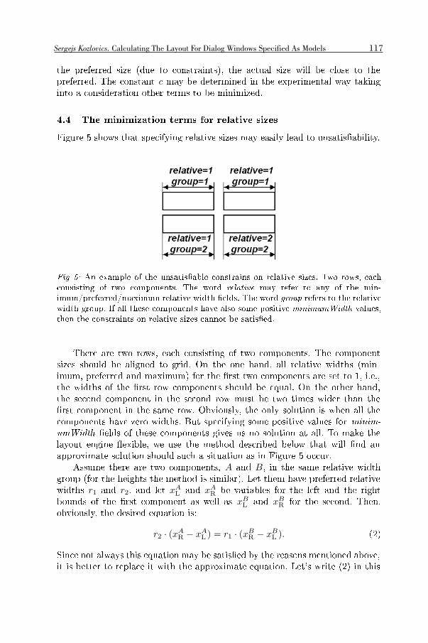
Sergejs Kozlovics. Calculating The Layout For Dialog Windows Specified As Models
c
A B
r1 r2 xAL xA
R
xBL xB
R
r2 · (xAR − xA
L ) = r1 · (xBR − xB
L ).
117
LURaksti787-datorzinatne.indd 117LURaksti787-datorzinatne.indd 117 23.10.2012 12:02:4823.10.2012 12:02:48

r2 · (xAR − xA
L )− r1 · (xBR − xB
L ) ≈ 0.
(r2 · (xA
R − xAL )− r1 · (xB
R − xBL ))2
.
k k · r1 k · r2r1 r2
(r1r2
)←
( r1r1+r2r2
r1+r2
)
(C1, r1, s1), (C2, r2, s2), . . . , (Cn, rn, sn) riCi
si
k
k ← max
{siri
}.
Ci
k · ri
(Ci, ri, si) risi ri si
k max min {si/ri}
xCL − xC
LM ≥ ,xCRM − xC
R ≥ .
C
xCLB − xC
L ≥ ,xCR − xC
RB ≥ .
118 COMPUTER SCIENCE AND INFORMATION TECHNOLOGIES
LURaksti787-datorzinatne.indd 118LURaksti787-datorzinatne.indd 118 23.10.2012 12:02:4923.10.2012 12:02:49
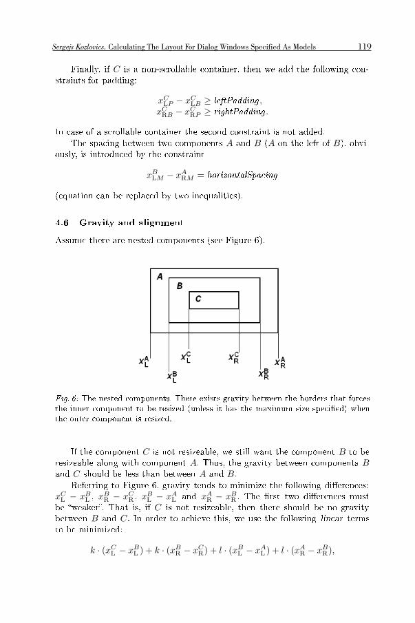
Sergejs Kozlovics. Calculating The Layout For Dialog Windows Specified As Models
C
xCLP − xC
LB ≥ ,xCRB − xC
RP ≥ .
A B A B
xBLM − xA
RM =
C BA B
C A B
xCL − xB
L xBR − xC
R xBL − xA
L xAR − xB
R
CB C
k · (xCL − xB
L ) + k · (xBR − xC
R) + l · (xBL − xA
L ) + l · (xAR − xB
R),
119
LURaksti787-datorzinatne.indd 119LURaksti787-datorzinatne.indd 119 23.10.2012 12:02:5023.10.2012 12:02:50

k < l C A(xC
L − xAL ) + (xA
R − xCR) k < l
B nk n
xCL − xB
L ≥ 0,xBR − xC
R ≥ 0,xBL − xA
L ≥ 0,xAR − xB
R ≥ 0.
xBL − xA
L = 0,
A B
c · ((xBL − xA
L )− (xAR − xB
R))2
xBL − xA
L ≥ 0,xAR − xB
R ≥ 0.
G = (V,E)V = {s, v0, v1, . . . , vn−1} vi
xi s E
E = {(vi, vj) : xi − xj ≥ dij ≥ mij }
∪{(s, v0), (s, v1), . . . , (s, vn−1)}.
dij (1)
xj − xi ≤ −dij .
120 COMPUTER SCIENCE AND INFORMATION TECHNOLOGIES
LURaksti787-datorzinatne.indd 120LURaksti787-datorzinatne.indd 120 23.10.2012 12:02:5123.10.2012 12:02:51
Sergejs Kozlovics. Calculating The Layout For Dialog Windows Specified As Models
(vi, vj) −dij(s, vi)
Gmij dij G
mij
dij
O(V 3)
121
LURaksti787-datorzinatne.indd 121LURaksti787-datorzinatne.indd 121 23.10.2012 12:02:5123.10.2012 12:02:51

:Formcaption="Sample form"
:HorizontalBox
:HorizontalBoxhorizontalAlignment=RIGHT
:VerticalBox:VerticalBox
verticalAlignment=TOP:HorizontalBox
:Labelcaption="E-mail:"
:InputFieldtext="[email protected]"
:ListBox :Itemvalue="[email protected]"
:Itemvalue="[email protected]"
:Buttoncaption="Add"
:Buttoncaption="Remove"
:Buttoncaption="OK"
:Buttoncaption="Cancel"defaultButtoncancelButton
selectedItem
122 COMPUTER SCIENCE AND INFORMATION TECHNOLOGIES
LURaksti787-datorzinatne.indd 122LURaksti787-datorzinatne.indd 122 23.10.2012 12:02:5323.10.2012 12:02:53

Sergejs Kozlovics. Calculating The Layout For Dialog Windows Specified As Models 123
LURaksti787-datorzinatne.indd 123LURaksti787-datorzinatne.indd 123 23.10.2012 12:02:5423.10.2012 12:02:54

124 COMPUTER SCIENCE AND INFORMATION TECHNOLOGIES
LURaksti787-datorzinatne.indd 124LURaksti787-datorzinatne.indd 124 23.10.2012 12:02:5523.10.2012 12:02:55

Frequency Computable Relations �
Madara Augstkalne, Anda Berina, Rusins Freivalds,
Institute of Mathematics and Computer Science, University of Latvia,Raina Bulvaris 29, Riga, LV-1459, Latvia
Abstract. A transducer is a finite-state automaton with an input andan output. We compare possibilities of nondeterministic and probabilis-tic transducers, and prove several theorems which establish an infinitehierarchy of relations computed by these transducers. We consider onlyleft-total relations (where for each input value there is exactly one al-lowed output value) and Las Vegas probabilistic transducers (for whichthe probability of any false answer is 0). It may seem that such limita-tions allow determinization of these transducers. Nonetheless, quite theopposite is proved; we show a relation which can only be computed byprobabilistic (but not deterministic) transducers, and one that can onlybe computed by nondeterministic (but not probabilistic) transducers.Frequency computation was introduced by Rose and McNaughton inearly sixties and developed by Trakhtenbrot, Kinber, Degtev, Wechsung,Hinrichs and others. It turns out that for transducers there is an infi-nite hierarchy of relations computable by frequency transducers and thishierarchy differs very much from similar hierarchies for frequency com-putation by a) Turing machines, b) polynomial time Turing machines,c) finite state acceptors.
1 Introduction
Frequency computation was introduced by G. Rose [13] as an attempt to havea deterministic mechanism with properties similar to probabilistic algorithms.The definition was as follows. A function f : w → w is (m,n)-computable, where1 ≤ m ≤ n, iff there exists a recursive function R: wn → wn such that, for alln-tuples (x1, · · · , xn) of distinct natural numbers,
card{i : (R(x1, · · · , xn))i = f(xi)} ≥ m.
R. McNaughton cites in his survey [12] a problem (posed by J. Myhill)whether f has to be recursive if m is close to n. This problem was answeredby B.A. Trakhtenbrot [14] by showing that f is recursive whenever 2m > n. Onthe other hand, in [14] it was proved that with 2m = n nonrecursive functionscan be (m,n)-computed. E.B. Kinber extended the research by considering fre-quency enumeration of sets [9]. The class of (m,n)-computable sets equals theclass of recursive sets if and only if 2m > n.
� The research was supported by Grant No. 09.1570 from the Latvian Council ofScience.
SCIENTIFIC PAPERS, UNIVERSITY OF LATVIA, 2012. Vol. 787COMPUTER SCIENCE AND INFORMATION TECHNOLOGIES 125–135 P.
LURaksti787-datorzinatne.indd 125LURaksti787-datorzinatne.indd 125 23.10.2012 12:02:5623.10.2012 12:02:56

For resource bounded computations, frequency computability behaves dif-ferently. For example, it is known that whenever n′ − m′ > n − m, under anyreasonable resource bound there are sets which are (m′, n′)-computable, but not(m,n)-computable. However, for finite automata, an analogue of Trakhtenbrot’sresult holds: the class of languages (m,n)-recognizable by deterministic finiteautomata equals the class of regular languages if and only if 2m > n. Con-versely, for 2m ≤ n, the class of languages (m,n)-recognizable by deterministicfinite automata is uncountable for a two-letter alphabet [1]. When restricted toa one-letter alphabet, every (m,n)-recognizable language is regular. This wasalso shown by Kinber.
Frequency computations became increasingly popular when the relation be-tween frequency computation and computation with a small number of querieswas discovered [11, 6, 2, 3].
We considered problems similar to those in the classical papers [14, 9, 1] forfinite-state transducers. We found the situation to be significantly different.
A finite state transducer is a finite state machine with two tapes: an inputtape and an output tape. These tapes are one-way, i.e. the automaton neverreturns to the symbols once read or written. Transducers compute relationsbetween the input words and output words. A deterministic transducer producesexactly one output word for every input word processed.
In this paper we consider advantages and disadvantages of nondeterministic,deterministic, frequency and probabilistic transducers. Obviously, if a relation issuch that several output words are possible for the same input word, then therelation cannot be computed by a deterministic transducer. For this reason, inthis paper we restrict ourselves to relations which produce exactly one outputword for every input word processed.
Definition 1. We say that a relation R(x, y) is left-total, if for arbitrary x thereis exactly one y satisfying R(x, y).
Probabilistic algorithms may be of several types: those allowing errors ofall types, Monte Carlo, Las Vegas, etc. Since our relations produce exactly oneoutput word for every input word processed, it was natural to consider onlyLas Vegas transducers, i.e. probabilistic transducers for which the probabilityof every false answer is 0. It follows immediately from the definition that ev-ery relation computed by such a probabilistic transducer can be computed bya nondeterministic transducer as well. We prove below that nondeterministictransducers are strictly more powerful than Las Vegas transducers.
The zero probability of all possible false results of a probabilistic transducerhas another unexpected consequence. It turns out that only recursive relationsof small computational complexity can be computed by probabilistic transducerswith a probability, say, 1
4 or 17 . Hence a natural question arises, whether every
rational number 0 ≤ p ≤ 1 can be the best probability to compute some relationby a probabilistic finite-state transducer. It turns out that it is not the case. Weshow examples of relations that can be computed by probabilistic finite-statetransducers with probabilities 1
2 ,13 ,
14 , etc. and not better. We believe that no
other best probabilities can exist for relations of the type considered by us.
126 COMPUTER SCIENCE AND INFORMATION TECHNOLOGIES
LURaksti787-datorzinatne.indd 126LURaksti787-datorzinatne.indd 126 23.10.2012 12:02:5623.10.2012 12:02:56

Madara Augstkalne, Andra Beriņa, Rūsiņš Freivalds. Frequency Computable Relations
This hierarchy of relations turns out to be related to the number of symbols ofhelp needed for deterministic finite-state transducers that take advice to computethese relations.
2 Definitions
We use standard definitions of deterministic, nondeterministic and probabilistictransducers, which are well-established in theoretical computer science literature[5]. Our model is slightly different in the regard that we allow multiple outputsymbols for each transition, however it can be easily seen that the expressivepower of transducer is unaffected.
Definition 2. A nondeterministic transducer D is a six-tuple 〈Q,Σ,Δ, δ, q0, F 〉,which satisfies the following conditions:
– Q is a finite set, whose members are called states of D. q0 ∈ Q is called theinitial state of D,
– Σ is a set of input symbols of D and is called the input alphabet,– Δ is a set of output symbols of D and is called the output alphabet,– δ is a relation from Q × (Σ ∪ {ε}) to Q ×Δ∗. Each tuple ((q, α), (p, β)) is
called a transition rule of D,– F ⊆ Q is the set of accepting or final states of D
A transducer operates in discrete time t = 1, 2, 3 . . . and handles two one-way tapes, where one is read-only input tape and contains a string from theinput alphabet Σ and second is write-only output tape with finite output alphabetΔ.
The computation begins at the start state q0. The computation from state qproceeds by reading symbol α from the input tape, following a suitable transitionrule ((q, α), (p, β)) (the new state being p) and writing the corresponding outputβ to the output tape. The only exception is so called ε-transition ((p, ε), (q, β)),where the transducer changes the state and possibly writes an output withoutreading an input symbol.
We consider all our transducers as machines working infinetely long. At everymoment, let x be the word having been read from the input tape up to this mo-ment, and let y be the word written on the output tape up to this moment. Thenwe say that the pair (x, y) belongs to the relation computed by the transducer.
Definition 3. A deterministic transducer is a nondeterministic transducer suchthat transition relation δ is a function, i.e., for each input state and each inputsymbol the corresponding output state and output symbol is uniquely determinedaccording to the transition table δ.
Definition 4. A probabilistic transducer is a transducer of the form〈Q,Σ,Δ, Ψ, q0, F 〉 where the transition function Ψ is probabilistic, i.e., for everystate q and input symbol α, output state p and output symbol β there is an
127
LURaksti787-datorzinatne.indd 127LURaksti787-datorzinatne.indd 127 23.10.2012 12:02:5623.10.2012 12:02:56

associated probability with which transition occurs. We furthermore stipulate thatprobabilities of all transition from any fixed pair of input state and input symbolmust sum to one.
Definition 5. We say that a probabilistic transducer A computes a left-totalrelation R with probability p if for arbitrary pair (x, y) ∈ R when A works oninput x the probability to go into an accepting state having produced the outputy is no less than p.
Definition 6. We say that a probabilistic transducer A is a Las Vegas trans-ducer computing a left-total relation R with probability p if for arbitrary pair(x, y) ∈ R when A works on input x the probability to go into an accepting statehaving produced the output y is no less than p, and the probability to go into anaccepting state having produced the output other than y equals 0.
Since we consider in our paper only left-total relations and since our proba-bilistic transducers are Las Vegas, it easily follows that the transducer for arbi-trary x and for arbitrary α ∈ {α1, α2, . . . , αn} either produces a correct outputy or reaches a non-accepting state.
Definition 7. A frequency transducer with parameters (m,n) is a transducerwith n input tapes and n output tapes. Every state of the transducer is defined as(a1, a2, · · · , an)-accepting where each ai ∈ { accepting , nonaccepting }. We saythat a left-total relation R is (m,n)-computed by the transducer if for arbitraryn-tuple of pairwise distinct input words (x1, x2, · · · , xn) there exist at least mdistinct values of xi such that the i-th output yi satisfies (xi, yi) ∈ R.
Please notice that we do not demand the state of the frequency transducerto be all-accepting after the reading of the input words. This allows us introducea counterpart of Las Vegas transducer.
Definition 8. A Las Vegas frequency transducer with parameters (m,n) is atransducer with n input tapes and n output tapes. Every state of the transducer isdefined as (a1, a2, · · · , an)-accepting where each ai ∈ { accepting , nonaccepting }.We say that a left-total relation R is (m,n)-computed by the transducer if forarbitrary n-tuple of pairwise distinct input words (x1, x2, · · · , xn): 1) there existat least m distinct values of xi such that the i-th output yi satisfies (xi, yi) ∈ R,and 2) if a result yi is produced on any output tape i and the current state of thetransducer is (a1, a2, · · · , ai−1, accepting, ai+1, · · · , an)-accepting, then R(xi, yi).
We consider frequency transducers like all other transducers as machinesworking infinitely long. At every moment, let x be the word having been readfrom the input tape up to this moment, and let y be the word written (andaccepted) on the output tape up to this moment. Then we say that the pair(x, y) belongs to the relation computed by the transducer. However, in the casewhen the input alphabet contains less than n letters, there is a problem how todefine (m,n)-computation correctly.
128 COMPUTER SCIENCE AND INFORMATION TECHNOLOGIES
LURaksti787-datorzinatne.indd 128LURaksti787-datorzinatne.indd 128 23.10.2012 12:02:5623.10.2012 12:02:56

Madara Augstkalne, Andra Beriņa, Rūsiņš Freivalds. Frequency Computable Relations
Definition 9. We say that a frequency transducer is performing a strong (m,n)-computation if at moments when all the input words (x1, x2, · · · , xn) are distinctthere exist at least m distinct values of xi such that the i-th output yi satisfies(xi, yi) ∈ R.
Definition 10. We say that a frequency transducer is performing a weak (m,n)-computation with parameters (b1, b2, · · · bn), where b1, b2, · · · bn are distinct inte-gers, if the transducer is constructed in such a way that in the beginning of thework the transducer reads the first b1 symbols from the input word x1, the firstb2 symbols from the input word b2, · · · , the first bn symbols from the input wordxn and at all subsequent moments reads exactly 1 new symbol from every inputtape. This ensures that at all moments the input words (x1, x2, · · · , xn) are dis-tinct. There is no requirement of the correctness of the results when the lengthof input words is (b1, b2, · · · bn) but at all moments afterwards there exist at leastm distinct values of xi such that the i-th output yi satisfies (xi, yi) ∈ R.
3 Frequency transducers
First of all, it should be noted that a frequency transducer does not specifyuniquely the relation computed by it. For instance, a transducer with 3 inputtapes and 3 output tapes (2, 3)-computing the relation
R(x, y) =
⎧⎨⎩
true, if x = y and x = 258714,true, if y = 0 and x = 258714,false, if otherwise.
can output y = x for all possible inputs and, nonetheless, the result is alwayscorrect for at least 2 out of 3 inputs since the inputs always distinct. Pleasenotice that the program of the frequency transducer does not contain the”magical” number 258714. Hence the number of states for an equivalent deter-ministic transducer can be enormously larger.
Theorem 1. There exists a strong finite-state frequency transducer (1, 2)-computinga continuum of left-total relations.
Proof. Consider the following frequency transducer with 2 input tapes and 2output tapes. If the inputs x1 and x2 are such that x1 is an initial fragment ofx2, then the output y1 equals x1, and y2 = 0. If the inputs x1 and x2 are suchthat x2 is an initial fragment of x1, then the output y2 equals x2, and y1 = 0.In all the other cases y1 = y2 = 0.
Let R be a relation defined by taking an arbitrary infinite sequence ω of zerosand ones, and defining
R(x, y) =
⎧⎨⎩
true, if y = x and x is an initial fragment of ω,true, if y = 0 and x is not an initial fragment of ω,false, if otherwise.
There is a continuum of such sequences and a continuum of the correspondingrelations. Each of them is (1, 2)-computed by the frequency transducer. ��
129
LURaksti787-datorzinatne.indd 129LURaksti787-datorzinatne.indd 129 23.10.2012 12:02:5623.10.2012 12:02:56

Theorem 2. If 2m > n and there exists a strong finite-state frequency trans-ducer (m,n)-computing a left-total relation R then R can also be computed by adeterministic finite-state transducer.
Proof. Let R be a left-total relation and A be a strong finite-state frequencytransducer (m,n)-computing it. Let Q be (another) left-total relation (m,n)-computed by the same transducer A. Let x1, x2, · · · , xk be distinct input wordssuch that the pairs (x1, y
′1), (x2, y
′2), · · · , (xk, y
′k) are in R, the pairs (x1, y
′′1 ),
(x2, y′′2 ), · · · , (xk, y
′′k ) are in Q, and y′1 = y′′1 , y
′2 = y′′2 , · · · , y′k = y′′k . What happens
if k ≥ n and the transducer gets an input-tuple containing only values from{x1, x2, · · · , xk}? The transducer has to output at least m correct values for Rand at least m correct values for Q which is impossible because 2m > n. Acareful count shows that k ≤ 2n− 2m .
Hence for arbitrary given relation R (m,n)-computable by A there is a con-stant k such that any relation Q (m,n)-computable by A differs from R on nomore that k0 pairs (x, y). Let Q0 be one of the relations where indeed k such pairsexist, and let (x1, y
′1), (x2, y
′2), · · · , (xk, y
′k) and (x1, y
′′1 ), (x2, y
′′2 ), · · · , (xk, y
′′k ) be
these pairs. Of course, there is no algorithm to construct k and Q0 effectively,but they cannot fail to exist. For arbitrary x the value of y such that (x, y) ∈ Rcan be calculated effectively using n-tuples of input words involving the inputwords x1, x2, · · · , xk and remembering that no relation computed by A can dif-fer from R and from Q0 in more than k values. Since A is a finite automaton,the standard cut-and-paste arguments show that this computation needs onlyinput words which differ from x only on the last d digits where d is a suitableconstant. ��Theorem 3. There exists a left-total relation R (2, 3)-computed by a weak finite-state Las Vegas frequency transducer and not computed by any deterministicfinite-state transducer.
Proof. We consider the relation
R(x, y) =
⎧⎪⎪⎨⎪⎪⎩
true, if y = 1|x| and | x |≡ 0(mod3),true, if y = 1|x| and | x |≡ 1(mod3)true, if y = 1|x|−1 and | x |≡ 2(mod3)false, if otherwise.
The weak finite-state Las Vegas frequency (2, 3)-transducer starts with read-ing 1 symbol from the first input tape, 2 symbols from the second input tape and3 symbols from the third input tape and reads exactly 1 symbol from each inputtape at any moment. Hence at any moment the transducer has no more than oneinput word xi with | xi |≡ 2(mod3). To have a correct result for the other twoinput words, it suffices to keep the length of the output being equal the lengthof the corresponding input. In case if the length of the input is | xi |≡ 2(mod3),the state becomes non accepting.
The relation cannot be computed by a deterministic transducer because thelength of the output y decreases when the length of of the input increases from3k + 1 to 3k + 2. ��
130 COMPUTER SCIENCE AND INFORMATION TECHNOLOGIES
LURaksti787-datorzinatne.indd 130LURaksti787-datorzinatne.indd 130 23.10.2012 12:02:5623.10.2012 12:02:56

Madara Augstkalne, Andra Beriņa, Rūsiņš Freivalds. Frequency Computable Relations
This proof can easily be extended to prove the following Theorem 4.
Theorem 4. If m < n then there exists a left-total relation R (m,n)-computedby a weak finite-state Las Vegas frequency transducer and not computed by anydeterministic finite-state transducer.
Theorem 5. There exists a left-total relation R (2, 4)-computed by a weak finite-state Las Vegas frequency transducer and not computed by any finite-state (1, 2)-frequency transducer.
Proof. We consider the relation
R(x, y) =
⎧⎪⎪⎪⎪⎪⎪⎪⎪⎪⎪⎪⎪⎪⎪⎨⎪⎪⎪⎪⎪⎪⎪⎪⎪⎪⎪⎪⎪⎪⎩
true, if y = 1|x| and | x |≡ 0(mod9),true, if y = 1|x| and | x |≡ 3(mod9),true, if y = 1|x| and | x |≡ 4(mod9),true, if y = 1|x| and | x |≡ 6(mod9),true, if y = 1|x| and | x |≡ 8(mod9),true, if y = 0 and | x |≡ 1(mod9),true, if y = 0 and | x |≡ 2(mod9),true, if y = 0 and | x |≡ 5(mod9),true, if y = 0 and | x |≡ 7(mod9),false, if otherwise.
(1) The weak finite-state Las Vegas frequency (2, 4)-transducer starts with read-ing 1 symbol from the first input tape, 2 symbols from the second input tapeand 3 symbols from the third input tape, 4 symbols from fourth input tape andreads exactly 1 symbol from each input tape at any moment. The transduceralways outputs yi = 1|xi| on the i-th output tape. Since the transducer can countthe length of the input modulo 9, the false outputs (in cases | xi | congruent to1,2,5 or 7 (mod 9)) are not accepted and the transducer is Las Vegas.
At every moment the lengths of the input words are k, k + 1, k + 2, k + 3 forsome natural k. At least two of them are congruent to 0,3,4,6 or 8 (mod 9).
(2) Assume that the relation is (1, 2)-computed by a transducer performinga weak (1, 2)-computation with parameters (b1, b2). Whatever the difference d =b2 − b1, there exists a value of s such that both s+ b1 and s+ b2 are congruentto 1,2,5 or 7 (mod 9). Hence the transducer produces two wrong results on thepair 1s+b1 , 1s+b2 in contradiction with the (1, 2)-computability. ��
4 Nonconstructive methods for frequency transducers
Unfortunately, it is not clear how to generalize the explicit construction of therelation R(x, y) in Theorem 5 to prove distinction between (m,n)-computabilityand (km, kn)-computability for weak finite-state frequency transducers. Luckily,there is a non-constructive method to do so. This method is based on usage ofalgorithmic information theory.
131
LURaksti787-datorzinatne.indd 131LURaksti787-datorzinatne.indd 131 23.10.2012 12:02:5623.10.2012 12:02:56

Definition 11. We define a transformation I which takes words x ∈ {0, 1}∗ intoI(x) ∈ {0, 1}∗ by the following rule. Every symbol 0 is replaced by 1100110100and every symbol 1 is replaced by 1011001010.
Definition 12. We define a transformation J which takes words x ∈ {0, 1}∗into J(x) ∈ {0, 1}∗ by the following rule. Every symbol 0 is replaced by 0100110100and every symbol 1 is replaced by 0011001010.
Lemma 1. For arbitrary x ∈ {0, 1}∗ the result of the transformation I is a wordI(x) such that | I(x) |= 10 | x |, and I(x) contains equal number of zeros andones.
Lemma 2. For arbitrary x ∈ {0, 1}∗ the result of the transformation J is aword J(x) such that | J(x) |= 10 | x |, and every subword y of J(x) such that| J(x) |= 10 contains no more than 5 symbols 1.
Definition 13. We define a transformation K which takes words x ∈ {0, 1}∗into a 2-dimensional array
K(x) =
⎛⎜⎜⎝
K11 K12 · · · K1n
K21 K22 · · · K2n
· · · · · · · · · · · ·Kn1 Kn2 · · · Knn
⎞⎟⎟⎠
of size 10 | x | × 10 | x | by the following rule. The first row (K11 K12 · · · K1n
)copies I(x). Every next row is a cyclic copy of the preceding one:
(Ks1 Ks2 · · · Ksn
)=(K(s−1)2 K(s−1)3 · · · K(s−1)1
).
Definition 14. We define a transformation L which takes words x ∈ {0, 1}∗into a 2-dimensional array
L(x) =
⎛⎜⎜⎝
L11 L12 · · · L1n
L21 L22 · · · L2n
· · · · · · · · · · · ·Ln1 Ln2 · · · Lnn
⎞⎟⎟⎠
of size 10 | x | × 10 | x | by the following rule. The first row (L11 L12 · · · L1n
)copies J(x). Every next row is a cyclic copy of the preceding one:
(Ls1 Ls2 · · · Lsn
)=(L(s−1)2 L(s−1)3 · · · L(s−1)1
).
There is a dichotomy: 1) either there exist 4 rows (say, with numbers b1, b2, b3,b4) inK(x) such that in every column Z such that among the valuesK(b1)z,K(b2)z,K(b3)z,K(b4)z there are exactly 2 zeros and 2 ones, or 2) for arbitrary 4 rows (with
132 COMPUTER SCIENCE AND INFORMATION TECHNOLOGIES
LURaksti787-datorzinatne.indd 132LURaksti787-datorzinatne.indd 132 23.10.2012 12:02:5623.10.2012 12:02:56

Madara Augstkalne, Andra Beriņa, Rūsiņš Freivalds. Frequency Computable Relations
numbers b1, b2, b3, b4 in K(x)) there is a column z such that among the valuesK(b1)z,K(b2)z,K(b3)z,K(b4)z there are at least 3 values equal to 1. (Please remem-ber that by Lemma 2 the total number of zeros and ones in every row is thesame.) We will prove that if the Kolmogorov complexity of x is maximal andthe length of x is sufficiently large then the possibility 1) does not exist.
Lemma 3. If n is sufficiently large and x is a Kolmogorov-maximal word oflength n then for arbitrary 4 rows (with numbers b1, b2, b3, b4 in K(x)) there isa column z such that among the values K(b1)z,K(b2)z,K(b3)z,K(b4)z there are atleast 3 values equal to 1.
Proof. Assume from the contrary that there exist 4 rows (say, with num-bers b1, b2, b3, b4) in K(x) such that in every column z such that among thevalues K(b1)z,K(b2)z,K(b3)z,K(b4)z there are exactly 2 zeros and 2 ones. By def-inition of K, K(bi)z = K1(z+bi−1). Hence every assertion ”among the valuesK(b1)z,K(b2)z,K(b3)z,K(b4)z there are exactly 2 zeros and 2 ones” can be writtenas ”among the values K1(c1),K1(c2),K1(c3),K1(c4) there are exactly 2 zeros and2 ones” which is equivalent to ”among the values I(d1), I(d2), I(d3), I(d4) thereare exactly 2 zeros and 2 ones”.
Every value I(d) was obtained from a single letter in the word x. Namely,the letters I(10j + 1), I(10j + 2), · · · , I(10j + 10) were obtained from the j-thletterx(j) of x. I(10j + 1) = 1 both for x(j) being a or b. I(10j + 2) = 1 if x(j)equals a but not b. I(10j+3) = 1 if x(j) equals b but not a. Hence we introducea functional
h(x(j)) =
⎧⎪⎪⎨⎪⎪⎩
1 , if d ≡ 0(mod10)
x(j) , if d ≡ 1 or 4 or 5 or 7(mod10)x(j) , if d ≡ 2 or 3 or 6 or 8(mod10)0 , if d ≡ 9(mod10)
Using this functional we transform every assertion of ”among the valuesI(d1), I(d2), I(d3), I(d4) there are exactly 2 zeros and 2 ones” type into a Booleanformula ”among the values h(xj1), h(xj2), h(xj3), h(xj4) there are exactly 2 zerosand 2 ones”.
Let a set S of such Boolean formulas be given. We say that another formulaF is independent from the set S if F cannot be proved using formulas from theset S. For instance, if F contains a variable not present in any formula of S thenF is independent from S.
Take a large integer n and consider the set T of all binary words from {a, b}2n.There are 22n words in T . Let T1 be the subset of T containing all words withequal number of a’s and b’s. Cardinality of T1 equals 2
2n−o(n). The set S contains2n formulas but not all of them are independent. However, since each formulacontains only 4 variables, there are at least 2n
4 independent formulas in S. Applyone-by-one these independent formulas and removes from T1 all the words wheresome formula fails. Notice that application of a new formula independent fromthe preceding ones remove at least half of the words. Hence after all removalsno more than 2
3n2 −o(n) words remain. Effective enumeration of all the remaining
133
LURaksti787-datorzinatne.indd 133LURaksti787-datorzinatne.indd 133 23.10.2012 12:02:5723.10.2012 12:02:57

words and usage of Kolmogorov numbering as in Section 4 gives a method tocompress each x to a length not exceeding 3n
2 − o(n). This contradicts non-compressibility of Kolmogorov-maximal words. ��
Since independence of formulas in our argument was based only on the usedvariables the same argument proves the following lemma.
Lemma 4. If n is sufficiently large and x is a Kolmogorov-maximal word oflength n then for arbitrary 4 rows (with numbers b1, b2, b3, b4 in L(x)) there isa column z such that among the values L(b1)z, L(b2)z, L(b3)z, L(b4)z there are atleast 3 values equal to 1.
We are ready to prove the main theorem of this paper.
Theorem 6. There exists a left-total relation R (3, 6)-computed by a weak finite-state frequency transducer and not computed by any finite-state (2, 4)-frequencytransducer.
Proof. Consider the relation
R(x, y) =
⎧⎨⎩
true, if y = 1|x| and | x |≡ j(modn) and L1j = 0true, if y = 0 and | x |≡ j(modn) and L1j = 1false, if otherwise.
where L(x) is as described above. ��
References
1. Holger Austinat, Volker Diekert, Ulrich Hertrampf, Holger Petersen. Regular fre-quency computations. Theoretical Computer Science, vol. 330 No. 1, pp. 15–20,2005.
2. Richard Beigel, William I. Gasarch, Efim B. Kinber. Frequency computation andbounded queries. Theoretical Computer Science, vol. 163 No. 1/2, pp. 177–192,1996.
3. John Case, Susanne Kaufmann, Efim B. Kinber, Martin Kummer. Learning re-cursive functions from approximations. Journal of Computer and System Sciences,vol. 55, No. 1, pp. 183–196, 1997.
4. A.N.Degtev. On (m,n)-computable sets. Algebraic Systems, Edited by D.I. Molda-vanskij, Ivanovo Gos. Universitet, pp. 88–99, 1981.
5. Eitan Gurari. An Introduction to the Theory of Computation. Computer SciencePress, an imprint of E. H. Freeman, Chapter 2.2, 1989.
6. Valentina Harizanova, Martin Kummer, Jim Owings. Frequency computations andthe cardinality theorem. The Journal of Symbolic Logic, vol. 57, No. 2, pp. 682–687,1992.
7. Maren Hinrichs and Gerd Wechsung. Time bounded frequency computations. In-formation and Computation, vol. 139, pp. 234-257, 1997.
8. Richard M. Karp and Richard Lipton. Turing machines that take advice. L’ En-seignement Mathematique, vol. 28, pp. 191–209, 1982.
134 COMPUTER SCIENCE AND INFORMATION TECHNOLOGIES
LURaksti787-datorzinatne.indd 134LURaksti787-datorzinatne.indd 134 23.10.2012 12:02:5723.10.2012 12:02:57

Madara Augstkalne, Andra Beriņa, Rūsiņš Freivalds. Frequency Computable Relations
9. Efim B. Kinber. Frequency calculations of general recursive predicates and fre-quency enumeration of sets. Soviet Mathematics Doklady, vol. 13, pp. 873–876,1972.
10. Efim B. Kinber. Frequency computations in finite automata, Kibernetika, No. 2,pp. 7–15, 1976(Russian; English translation in Cybernetics 12 (1976) 179-187).
11. Martin Kummer. A proof of Beigel’s Cardinality Conjecture. The Journal of Sym-bolic Logic, vol. 57, No. 2, pp. 677–681, 1992.
12. Robert McNaughton. The Theory of Automata, a Survey. Advances in Computers,vol. 2, pp. 379–421, 1961.
13. Gene F. Rose. An extended notion of computability. Abstracts of InternationalCongress for Logic, Methodology and Philosophy of Science, p.14, 1960.
14. Boris A. Trakhtenbrot. On the frequency computation of functions. Algebra iLogika, vol. 2, pp.25–32, 1964 (Russian)
135
LURaksti787-datorzinatne.indd 135LURaksti787-datorzinatne.indd 135 23.10.2012 12:02:5723.10.2012 12:02:57
On fault-tolerance of Grover’s algorithm
Nikolajs Nahimovs, Alexander Rivosh, Dmitry Kravchenko
Abstract
Grover’s algorithm is a quantum search algorithm solving the un-structured search problem of size N in O(
√N) queries, while any clas-
sical algorithm needs O(N) queries [1].However, if the query transformation might fail (with probability
independent of the number of steps of the algorithm), then quantumspeed-up disappears: no quantum algorithm can be faster than a clas-sical exhaustive search by more than a constant factor [6].
In this paper we study the effect of a small number of failed queries.We show that k failed queries with a very high probability changethe number of actually executed steps of Grover’s algorithm from l to
O(
l√k
).
1 Introduction
Grover’s algorithm is a quantum search algorithm solving the unstructuredsearch problem in about π
4
√N queries [1]. It has been analysed in great
detail. The analysis has been mainly focused on the optimality and gen-eralization of the algorithm [4, 2, 3], as well as on fault-tolerance of thealgorithm to various kind of physical errors, such as decoherence or randomimperfections in either diffusion transformations or black box queries [8, 7].
In this paper we study fault-tolerance of Grover’s algorithm to logicalfaults, in our case failure of one or more query transformations. Regev andSchiff have shown [6] that if the query transformation fails with a fixedprobability (independent of the number of steps of the algorithm), thenquantum speed-up disappears: no quantum algorithm can be faster than aclassical exhaustive search by more than a constant factor.
We find it interesting to understand what happens if only a small numberof failed queries is allowed. We show that even a single failed query canstop the algorithm from finding any of marked elements. Remarkably, thisproperty does not depend on a number of marked elements. This makes thequantum case completely different from the classical case.
SCIENTIFIC PAPERS, UNIVERSITY OF LATVIA, 2012. Vol. 787COMPUTER SCIENCE AND INFORMATION TECHNOLOGIES 136–146 P.
LURaksti787-datorzinatne.indd 136LURaksti787-datorzinatne.indd 136 23.10.2012 12:02:5723.10.2012 12:02:57

Nikolajs Nahimovs, Alexander Rivosh, Dmitry Kravchenko. On fault-tolerance of Grover’s ..
A failure of a single ormultiple query transformations results in a numberof steps not being executed. We show that k failed queries with a veryhigh probability change the number of actually executed steps of Grover’s
algorithm from l to O(
l√k
).
2 Grover’s algorithm
Suppose we have an unstructured search space consisting of N elementsx1, . . . , xN ∈ {0, 1}. Our task is to find xi = 1 or to conclude that no suchx exists.
Grover’s algorithm starts with a state |ψstart〉 = 1√N
∑Ni=1 |i〉. Each step
of the algorithm consists of two transformations: Q – query transformationdefined as Q|i〉 = (−1)xi |i〉 and D – the inversion about average, defined as:
D =
⎡⎢⎢⎢⎣
−1 + 2N
2N . . . 2
N2N −1 + 2
N . . . 2N
. . . . . . . . . . . .2N
2N . . . −1 + 2
N
⎤⎥⎥⎥⎦ .
The state of the algorithm after t steps is |ψt〉 = (DQ)t|ψstart〉.Grover’s algorithm has been analysed in detail and many facts about
it are known. If there is one marked element, the probability of finding itby measuring |ψt〉 reaches 1 − o(1) for t = O(
√N). If there are k marked
elements, the probability of finding one of them by measuring |ψt〉 reaches1− o(1) for t = O(
√N/k).
3 Grover’s algorithm with errors
In this section we study the effect of small number of errors (omitted querytransformations) on the transformation sequence of the algorithm. We showthat an omission of a single or multiple query transformations is equivalentto replacing a number of steps (DQ transformation pairs) with an identitytransformation, that is performing a smaller number of steps.
Let l be a number of steps of the algorithm. We show that k � l uni-formly distributed independent errors change the transformation sequenceof the algorithm from (DQ)l to (DQ)L, where L is the random variable
with expectation O( lk ) and standard deviation O
(l√k
). Therefore, with a
very high probability the length of the resulting transformation sequence is
O(
l√k
)[5].
137
LURaksti787-datorzinatne.indd 137LURaksti787-datorzinatne.indd 137 23.10.2012 12:02:5723.10.2012 12:02:57
Our further analysis is focused on the omission of the query transforma-tion Q. However a very similar analysis can be done for an omission of theD transformation.
3.1 Omitting a single query
The transformation sequence of Grover’s algorithm is
DQDQ . . . DQ = (DQ)l.
If we omit a single query transformation the sequence changes to
(DQ)l1D(DQ)l2 ,
where l1 + l2 + 1 = l, orD(QD)l1(DQ)l2 .
As DD = QQ = I (this follows from the definitions of D and Q transforma-tions), the shortest subsequence will cancel a part of the longest subsequence.More precisely
l1 ≥ l2 : D(QD)l1(DQ)l2 = D(QD)l1−l2
l1 < l2 : D(QD)l1(DQ)l2 = D(DQ)l2−l1 .
Thus, a single omitted query transformation changes the transformation se-quence of the algorithm from (DQ)l to (DQ)O(|l1−l2|), decreasing the numberof successful steps.
Suppose the query transformation can be omitted on a random algorithmstep, that is l1 is a uniformly distributed random variable. The length ofthe resulting transformation sequence will also be a random variable. Simplecalculations show that it has mean l
2 +O(1) and variance l2
12 +O(l).
Corollary
A single omitted query transformation on the average will twice decreasethe number of successful steps of the algorithm (or will twice increase theaverage running time of the algorithm).
If the query transformation will be omitted right in the middle of thetransformation sequence (l1 = l2), the number of successful steps will be 0.That is the algorithm will leave the initial state unchanged.
138 COMPUTER SCIENCE AND INFORMATION TECHNOLOGIES
LURaksti787-datorzinatne.indd 138LURaksti787-datorzinatne.indd 138 23.10.2012 12:02:5723.10.2012 12:02:57
Nikolajs Nahimovs, Alexander Rivosh, Dmitry Kravchenko. On fault-tolerance of Grover’s ..
3.2 Omitting multiple queries
The transformation sequence of the algorithm is
DQDQ . . . DQ = (DQ)l.
If we omit k − 1 query transformations, the sequence changes to
(DQ)l1D(DQ)l2D . . . (DQ)lk−1D(DQ)lk ,
where l1 + l2 + . . .+ lk + (k− 1) = l. By regrouping the brackets we will get
(DQ)l1DD(QD)l2(DQ)l3DD(DQ)l4 . . . =
(DQ)l1(QD)l2(DQ)l3(DQ)l4 . . .
Transformations Q and D have the following commutativity property:
(QD)i(DQ)j = (DQ)j(QD)i.
Thus, the sequence can be rewritten as
(DQ)l1+l3+... (QD)l2+l4+... .
Therefore, k omitted query transformations change the transformation se-quence of the algorithm from (DQ)l to (DQ)O(l1−l2+l3−l4+...±lk).
We will show that in the continuous approximation case (positions oferrors have continuous uniform distributions and l1 + l2 + . . . + lk = l) thelength of the resulting transformation sequence is a random variable with
mean 0 (even k) or lk (odd k) and variance O
(l2
k
). These values perfectly
agree with numerical experiment results for discrete case.
Proof of the main result
Suppose we have k − 1 independent random variables X1, X2, . . . , Xk−1.Each Xi is uniformly distributed between 0 and l. That is the probabilitydensity function of Xi is
fXi(x) =
⎧⎪⎨⎪⎩
1l x ∈ [0, l]
0 x /∈ [0, l]
139
LURaksti787-datorzinatne.indd 139LURaksti787-datorzinatne.indd 139 23.10.2012 12:02:5723.10.2012 12:02:57

and the cumulative distribution function is
FXi(x) =
⎧⎪⎪⎪⎪⎪⎨⎪⎪⎪⎪⎪⎩
0 x < 0
xl x ∈ [0, l]
1 x > l
.
The above random variables split the segment [0, l] into k subsegmentsl1, l2, . . . , lk. The length of each subsegment is also a random variable.
Let us focus on the subsegment l1. Probability that l1 ≤ x is the proba-bility that at least one of Xi ≤ x. Thus, the cumulative distribution functionof l1 is
Fl1 = 1− (1− FX1)(1− FX2) . . . (1− FXk−1)
or
Fl1(x) =
⎧⎪⎪⎪⎪⎪⎨⎪⎪⎪⎪⎪⎩
0 x < 0
1− (1− xl )
k−1 x ∈ [0, l]
1 x > l
.
The probability density function of l1 is
fl1(x) =
⎧⎪⎨⎪⎩
k−1l (1− x
l )k−2 x ∈ [0, l]
0 x /∈ [0, l]
.
Knowing the probability density function of l1, we can calculate its meanand variance by using the following formulae:
E[X] =
∫ ∞
−∞x · fX(x)dx
E[X2] =
∫ ∞
−∞x2 · fX(x)dx
V ar[X] = E[X2]− E[X]2.
We leave out the details of calculation of integrals and give the results.
E[l1] =
∫ ∞
−∞x · fl1(x)dx =
∫ l
0xk − 1
l(1− x
l)k−2dx =
l
k
140 COMPUTER SCIENCE AND INFORMATION TECHNOLOGIES
LURaksti787-datorzinatne.indd 140LURaksti787-datorzinatne.indd 140 23.10.2012 12:02:5723.10.2012 12:02:57
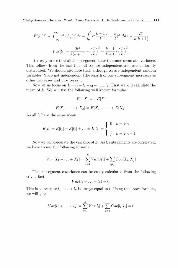
Nikolajs Nahimovs, Alexander Rivosh, Dmitry Kravchenko. On fault-tolerance of Grover’s ..
E[(l1)2] =
∫ ∞
−∞x2 · fl1(x)dx =
∫ l
0x2
k − 1
l(1− x
l)k−2dx =
2l2
k(k + 1)
V ar[l1] =2l2
k(k + 1)−(l
k
)2
=k − 1
k + 1·(l
k
)2
.
It is easy to see that all li subsegments have the same mean and variance.This follows from the fact that all Xi are independent and are uniformlydistributed. We should also note that, although Xi are independent randomvariables, li are not independent (the length of one subsegment increases asother decreases and vice versa) .
Now let us focus on L = l1 − l2 + l3 − ...± lk. First we will calculate themean of L. We will use the following well known formulae:
E[−X] = −E[X]
E[X1 + . . .+Xk] = E[X1] + . . .+ E[Xk].
As all li have the same mean
E[L] = E[l1]− E[l2] + . . .± E[lk] =
⎧⎪⎨⎪⎩
0 k = 2m
lk k = 2m+ 1
.
Now we will calculate the variance of L. As li subsegments are correlated,we have to use the following formula:
V ar[X1 + . . .+Xk] =k∑
i=1
V ar[Xi] +∑i �=j
Cov[Xi, Xj ]
The subsegment covariance can be easily calculated from the followingtrivial fact:
V ar(l1 + . . .+ lk) = 0.
This is so because l1+ . . .+ lk is always equal to l. Using the above formula,we will get:
V ar[l1 + . . .+ lk] =k∑
i=1
V ar[li] +∑i �=j
Cov[li, lj ] = 0
141
LURaksti787-datorzinatne.indd 141LURaksti787-datorzinatne.indd 141 23.10.2012 12:02:5723.10.2012 12:02:57

ork∑
i=1
V ar[li] = −∑i �=j
Cov[li, lj ].
As all li have the same mean and variance, they will also have the samecovariances Cov[li, lj ]. Using this fact, we will get
k · V ar[li] = −k(k − 1) · Cov[li, lj ]
or
Cov[li, lj ] = − 1
k − 1· V ar[li] = − 1
k + 1·(l
k
)2
.
Now let us return to the variance of L:
V ar[L] =k∑
i=1
V ar[li]±∑i �=j
Cov[li, lj ].
Covariance sign will depend on li and lj signs (whether they are the sameor not). More precisely:
Cov[−X,Y ] = Cov[X,−Y ] = −Cov[X,Y ]
Cov[−X,−Y ] = Cov[X,Y ].
If k = 2m, then m subsegments have plus sign and m subsegments haveminus sign. There are 2m(m−1) subsegment pairs with the same signs and2m2 subsegment pairs with opposite signs (we should count both (li, lj) and(lj , li) pairs). Thus, we can rewrite the formula as:
V ar[L] = k · V ar[li] + Cov[li, lj ] ·(2m(m− 1)− 2m2
)=
= k · V ar[li]− k · Cov[li, lj ] =
= k · V ar[li] +k
k − 1· V ar[li] =
= k · V ar[li] · k
k − 1.
If k = 2m+1, then m+1 subsegments have plus sign and m subsegmentshave minus sign. There are (m+ 1)m+m(m− 1) = 2m2 subsegment pairswith the same signs and 2(m + 1)m subsegment pairs with opposite signs.Thus, we can rewrite the formula as:
V ar[L] = k · V ar[li] + Cov[li, lj ] ·(2m2 − 2m(m− 1)
)=
142 COMPUTER SCIENCE AND INFORMATION TECHNOLOGIES
LURaksti787-datorzinatne.indd 142LURaksti787-datorzinatne.indd 142 23.10.2012 12:02:5723.10.2012 12:02:57

Nikolajs Nahimovs, Alexander Rivosh, Dmitry Kravchenko. On fault-tolerance of Grover’s ..
= k · V ar[li] + (k − 1) · Cov[li, lj ] =
= k · V ar[li]− V ar[li] =
= k · V ar[li] · k − 1
k.
Using O notation, we can rewrite both cases as O(k) · V ar[li] = O(l2
k
).
This ends the proof.
Corollary
We have shown that k− 1 omitted query transformations change the lengthof the transformation sequence of the algorithm from l to a random variable
with mean 0 (even k) or lk (odd k) and variance O
(l2
k
).
Using Chebyshev’s inequality, we can show that with 96% probability Lvalue will lie within five standard deviations from its mean [5]. For large k(but still k � l) even a more tight bound can be applied. In the next sectionwe will show that the probability distribution of L for large k is close to thenormal distribution. Thus, with 99.7% probability L will lie within threestandard deviations from the mean.
Therefore, with a very high probability the length of the resulting trans-
formation sequence changes from l to O(
l√k
).
4 Probability distribution of the median
In the previous section we have studied the following model. We have in-dependent random variables X1, X2, . . . , Xk−1. Each Xi is uniformly dis-tributed between 0 and l. The random variables split the segment [0, l] intok subsegments l1, l2, . . . , lk. Our task was to estimate L = l1 − l2 + l3 − l4 +. . . ± lk. Due to symmetry of li, L is equal to l
2 − Xm, where Xm is themedian of X1, X2, . . . , Xk−1, that is the point separating the higher half ofthe points from the lower half of the points.
In this section we will show that for a large number of uniformly dis-tributed random variables (points), the probability distribution of the me-dian is close to the normal distribution.
2k + 1 points
Let us consider a real number interval [−N ;N ] and 2k + 1 random points,each having a uniform distribution. Median is the point number k + 1.
143
LURaksti787-datorzinatne.indd 143LURaksti787-datorzinatne.indd 143 23.10.2012 12:02:5723.10.2012 12:02:57

Probability density of the median at position x, which is at the distance|x| from 0, can be expressed by the formula
fM (x) =(N − x)k (N + x)k
(2N)2k+1× (2k + 1)!
k!k!=
(N2 − x2
)k(2k)! (2k + 1)
(2N)2k+1 k!k!(1)
Using the Stirling approximation we can rewrite (1):
FM (x) ≈(N2 − x2
)k √4πk
(2ke
)2k(2k + 1)
(2N)2k+1√2πk
(ke
)k √2πk
(ke
)k =
(N2 − x2
)k(2k + 1)
2N2k+1√πk
(2)
=
(1− x2
N2
)k(2k + 1)
2N√πk
(3)
For large k we can approximate 2k + 1 with 2k:
fM (x) ≈(1− x2
N2
)k √k
N√π
(4)
For small xN values (4) can be approximated (applying 1− z ≈ e−z) by
fM (x) ≈
(e−
x2
N2
)k √k
N√π
=
√k
N√πe−k x2
N2 (5)
which corresponds to the normal distribution with mean 0 and variance N2
2k .
2k points
Let us consider a real number interval [−N ;N ] and 2k random points, eachhaving a uniform distribution. Median is the point number k.
Probability density of the median at position X, which is at the distance|X| from 0, can be expressed by the formula
fM (x) =(N − x)k−1 (N + x)k
(2N)2k× (2k)!
(k − 1)!k!=
(N2 − x2
)kk (2k)!
(2N)2k (N − x)k!k!(6)
144 COMPUTER SCIENCE AND INFORMATION TECHNOLOGIES
LURaksti787-datorzinatne.indd 144LURaksti787-datorzinatne.indd 144 23.10.2012 12:02:5723.10.2012 12:02:57

Nikolajs Nahimovs, Alexander Rivosh, Dmitry Kravchenko. On fault-tolerance of Grover’s ..
Using the Stirling approximation we can rewrite (6):
fM (x) ≈(N2 − x2
)kk√4πk
(2ke
)2k
(2N)2k (N − x)√2πk
(ke
)k √2πk
(ke
)k =
(N2 − x2
)k √k
N2k(N − x)√π
(7)
=
(1− x2
N2
)k √k(
1− xN
)N√π
(8)
For small XN values (8) can be approximated (applying 1− z ≈ e−z) by
fM (X) ≈
(e−
x2
N2
)k √k
(e−
xN
)N√π
=
√k
N√πe−k x2
N2+xN (9)
By multiplying (9) with e−14k , which for large k is close to 1, we will get
fM (x) ≈√k
N√πe−k x2
N2+xN− 1
4k =
√k
N√πe−k
(x− N2k
)2
N2 (10)
which corresponds to the normal distribution with mean N2k and variance
N2
2k .
5 Conclusions
We have shown that even a single failed query can change the resulting trans-formation sequence of the algorithm to an identity transformation. On theaverage, a single failed query will twice decrease the length of the resultingtransformation sequence. In case of k failed queries with a very high proba-bility the length of the resulting transformation sequence will be decreasedO(
√k) times.Similar argument can be applied to a wide range of other quantum query
algorithms, such as amplitude amplification, some variants of quantum walksand NAND formula evaluation, etc. That is to any quantum query algorithmfor which the transformation X applied between queries has the propertyX2 = I.
145
LURaksti787-datorzinatne.indd 145LURaksti787-datorzinatne.indd 145 23.10.2012 12:02:5823.10.2012 12:02:58

References
[1] Lov GroverA fast quantum mechanical algorithm for database search.Proceedings, 28th Annual ACM Symposium on the Theory of Comput-ing (STOC), May 1996, pages 212-219arXiv:quant-ph/9605043
[2] Cristof ZalkaGrovers quantum searching algorithm is optimal.Physical Review A, 60:2746-2751, 1999.arXiv:quant-ph/9711070
[3] G. Brassard et al.Quantum Amplitude Amplification and Estimation.arXiv:quant-ph/0005055
[4] C. Bennett et al.Strengths and Weaknesses of Quantum Computing.SIAM Journal on Computing (special issue on quantum computing) vol-ume 26, number 5, pages 1510-1523.arXiv:quant-ph/9701001
[5] R. Motwani, P. RaghavanRandomized Algorithms.Cambridge University Press, 1994.
[6] O. Regev, L. Schiff.Impossibility of a Quantum Speed-up with a Faulty Oracle.Proceedings of ICALP’2008, Lecture Notes in Computer Science,5125:773-781, 2008.http://www.cs.tau.ac.il/~odedr/papers/faultygrover.pdf
[7] D. Shapira et al.Effect of unitary noise on Grover’s quantum search algorithm.Phys. Rev. A volume 67, issue 4, April 2003
[8] Pil H. Song, ILki Kim.Computational leakage: Grover’s algorithm with imperfections.The European Physical Journal D - Atomic, Molecular, Optical andPlasma Physics volume 23, Number 2, May 2003, pages 299-303.arXiv:quant-ph/0010075
[9] John WatrousQuantum Computation.Lecture course ”CPSC 519/619”, University of Calgary, 2006.http://www.cs.uwaterloo.ca/ watrous/lecture-notes.html
146 COMPUTER SCIENCE AND INFORMATION TECHNOLOGIES
LURaksti787-datorzinatne.indd 146LURaksti787-datorzinatne.indd 146 23.10.2012 12:02:5823.10.2012 12:02:58

On languages not recognizable by One-wayMeasure Many Quantum Finite automaton �
Agnis Skuskovniks
Faculty of Computing, University of Latvia, Raina bulv. 19, Riga, LV-1586, Latvia,e-mail: [email protected]
Abstract. Measure Many Quantum Finite Automaton is not the strongestknown model of quantum automaton but, it is still an open questionwhat is the class of languages recognized by it when only bounded errorprobability is allowed. In this paper a natural class of ”word set” reg-ular languages are studied. A proof that in general case the class cannot be recognized by One-way model of Measure Many Quantum Finiteautomata is given.
Keywords: quantum computation, quantum automata, substring, MM-QFA
1 Introduction
Quantum finite automata (QFA) were introduced by several authors in differentways, and they can recognize different classes of languages. The least capableQFA are those (later called MO-QFA) introduced by C.Moore and J.Crutchfield[1]. More powerful notion of QFA (later called MM-QFA) was introduced byA.Kondacs and J.Watrous [2]. They introduced a 1-way and 2-way model ofMM-QFA.
A.Ambainis and R. Freivalds[3] examined 1-way model and found that forsome languages 1-way MM-QFA (1-QFA) can have exponential size advantagesover classical counterparts. They used a language in a single-letter alphabet toprove these advantages. A.Ambainis and other authors[4] improved the base ofthe exponent in these advantages by using more complicated languages in richeralphabets. Later A.Ambainis together with N.Nahimovs [5] simpified the con-struction and improved the exponent even more. Nonetheless A.Kondacs andJ.Watrous [2] showed that 1-QFA can only recognize regular languages, more-over, 1-QFA cannot recognize all the regular languages.
Future research had emphasis on 2-way automata because it was shown thatthey could recognize, all regular languages [6]. Also more general 1-way modelsof QFA where discovered[7][8], that could recognize all regular languages. Latermore general models of quantum automata were introduced and studied[9].
There are still open problems for 1-QFA model. There are two models of1-QFA: one that recognizes languages with bounded error probability and other� Supported by ESF project 2009/0216/1DP/1.1.1.2.0/09/APIA/VIAA/044.
SCIENTIFIC PAPERS, UNIVERSITY OF LATVIA, 2012. Vol. 787COMPUTER SCIENCE AND INFORMATION TECHNOLOGIES 147–152 P.
LURaksti787-datorzinatne.indd 147LURaksti787-datorzinatne.indd 147 23.10.2012 12:02:5823.10.2012 12:02:58
that recognizes languages with unbounded error probability. It has been shownthat unbounded model recognizes all and only stochastic languages[10]. It is notknown what is the language class recognized by 1-QFA with bounded error[11].The study of this class is interesting and challenging because it has been shownthat it is not closed under union or any standard Boolean operation[12].
Due to these facts the study of different natural language classes recogniz-able by 1-QFA is reasonable and justifiable even if stronger models of quantumautomata exist. In this paper we study a natural class of ”word set” languages.We show that in general case it cannot be recognized by 1-QFA with boundederror.
2 Preliminaries
2.1 1-Way Measure Many Quantum Finite Automata(1-QFA)
We define 1-QFA as follows[13].
Definition 21 A one-way quantum finite automaton A is specified by the finite(input) alphabet Σ, the finite set of states Q, the initial state q0, the sets Qa ⊆ Qand Qr ⊆ Q of accepting and rejecting states, respectively, with Qa ∩ Qr =empty − set, and the transition function
δ : Q× Γ ×Q→ C[0,1],
where Γ = Σ∪{#, $} is the tape alphabet of A, and # and $ are endmarkers notin Σ. The evolution (computation) of A is performed in the inner-product spacel2(Q), i.e., with the basis {|q〉|q ∈ Q}, using the linear operators Vσ, σ ∈ Γ ,defined by
Vσ(|q〉) =∑q′∈Q
σ(q, σ, q′)|q′〉,
which are required to be unitary.
In computation of A the so-called computational observable O is used thatcorresponds to the orthogonal decomposition
l2(Q) = Ea ⊕ Er ⊕ En,
where Ea = span{|q〉|q ∈ Qa} and Er = span{|q〉|q ∈ Qr} and En is theorthogonal complement of Ea ⊕ Er. Denote by Pp,p ∈ {a, r, n} the projectionoperator into the subspace Ep.A computation of A on an input #σ1 . . . σn$ proceeds as follows. The operatorV# is first applied to the starting configuration |q0〉 and then the observable Ois applied to the resulting configuration V#|q0〉. This observable projects V#|q0〉into a vector |ψ′〉 of one of the subspaces Ea, Er, En, with the probability equal tothe square of the norm of |ψ′〉. If |ψ′〉 inEa the input is accepted; if |ψ′〉 ∈ Ertheinput is rejected. If |ψ′〉 ∈ En, then, after the normalization of |ψ′〉, the operatorVσ1 is applied to |ψ′〉 and after that the observableO to the resulting vector. This
148 COMPUTER SCIENCE AND INFORMATION TECHNOLOGIES
LURaksti787-datorzinatne.indd 148LURaksti787-datorzinatne.indd 148 23.10.2012 12:02:5823.10.2012 12:02:58

Agnis Škuškovniks. On languages not recognizable by One-way Measure Many Quantum ..
process goes on. Operators Vσ1, Vσ2, . . . , Vσn are applied one after another, andafter each such application the measurement by the observable O is performed.In all cases the computation continues only if a projection into En occurs.When no termination occurs the computation can be seen as an application ofthe composed operator
V ′σnV
′σn−1 . . . V
′σ1|q0〉,
where V ′σ1 = PnVσ1.
In order to define formally the overall probability with witch an input is accepted(rejected) by a 1QFA A, we define the set VA = l2(Q)×C×C of so-called ”totalstates” of A, that will be used only with the following interpretation. A is at anytime during the computation in the state (ψ, pa, pr) if so far in its computation Aaccepted the input with probability pa, rejected with probability pr and neitherwith probability 1− pa − pr = ‖ψ‖2, and |ψ〉 is its current, unnormalized state.For each σ ∈ Γ the evolution of A, with respect to the total state, on an inputσ is given by the operator Tσ defined by
Tσ(ψ, pa, pr) → (PnVσψ, pa + ‖PaVσψ‖2, pr + ‖PrVσψ‖2).
For x = σ1σ2 . . . σn ∈ Γ ∗ let T#x$ = T$TσnTσn−1 . . . Tσ1T#. If T#x$(|q〉, 0, 0) =(ψ, pa, pr), then we say that A accepts x with probability pa and rejects withprobability pr. A 1QFA A is said to accept a language L with probability 1
2 +ε, ε > 0, if it accepts any x ∈ L with probability at least 1
2 + ε and rejects anyx /∈ L with probability at least 1
2 + ε. If there is an ε > 0 such that A accepts Lwith probability at least 1
2 + ε,then L is said to be accepted by A with bounded-error probability. L is said to be accepted with unbounded error probability ifx ∈ L is accepted with probability at least 1
2 and x /∈ L rejected with probabilityat least 1
2 .On VA we define a ”norm” ‖ · ‖u as follows
‖(ψ, pa, pr)‖u =12(‖ψ‖+ |pa|+ |pr|)
and let D = {v ∈ VA|‖v‖u ≤ 1}. D contains all global states of A.
2.2 A useful lemma
Consider the following lemma
Lemma 21 If |u〉 and |v〉 are vectors such that for a linear operator A, reals0 < ε < 1 and μ > 0,‖A(u− v)‖ < ε, and ‖v‖, ‖u‖,‖Au‖, ‖Av‖ are in [μ, μ+ ε],then there is a constant c, that does not depend on ε, such that ‖u− v‖ < cε
14 .
For proof look in [2]
149
LURaksti787-datorzinatne.indd 149LURaksti787-datorzinatne.indd 149 23.10.2012 12:02:5823.10.2012 12:02:58

3 Recognition of ”word set” language class
Given a finite alphabetA and a finite set of words in this alphabet {w1, w2, . . . , wk},consider the language class that consists of finite words {w1, w2, . . . , wk}∗.
Due to the properties of nondeterministic automata(NFA) it is easy to seethat a NFA that recognizes language from this class can easily be constructed.Language that is recognizable by NFA is regular, so languages in ”word set”language class are regular as well.
Theorem 31 Given a language S = {w1, w2, . . . , wk}∗ it is not possible in gen-eral case to build a 1-QFA that recognizes this language.
Proof. Lets look at the language S1 = {x|x ∈ [{0, 1}61] ∪ [{0, 1}81]}∗ and thelength of the words are greater than 56 (so that each word length could be puttogether by parts of length 7 and 9) in other words, language consists of all finitewords of length l = 7 ∗ a + 9 ∗ b that end with 1 and other symbols are from{0, 1}.It is easy to see that this language consists of subset of words from {0, 1}∗1language. Restrictions for determining the subset are: the word length is graterthan 56 and there is no substring that consists of more than 8 following zeros.A.Kondacs and J.Watrous [2] state that:
Theorem 32 The regular language L0 = {0, 1}∗0 cannot be recognized by a1QFA with bounded-error probability.
Proof. The proof is by contradiction. Let A= 〈Q,Σ, δ, q0, Qa, Qr〉 be a 1QFArecognizing the language L0. To each x = σ1 . . . σn ∈ Γ ∗ we assign the state
|ψx〉 = V ′σn . . . V
′σ1|q0〉
and let μ = infw∈{0,1}∗{‖ψ#w‖}. For each w ∈ {0, 1}∗, w0 ∈ L0 and w1 /∈ L0.If μ = 0, then clearly A cannot recognize L0 with bounded-error probability12 + ε. Let us therefore assume that μ > 0. For any ε > 0 there is a w such that‖ψ#w‖ < μ+ ε, and also ‖ψ#wy‖ ∈ [μ, μ+ ε] for any y ∈ {0, 1}∗. In particular,for any m > 0
‖V ′m1 |ψ#w0〉‖ ∈ [μ, μ+ ε). (1)
This implies that the sequence {V ′i1 |ψ#w0〉}∞i=0 is bounded in the finite dimen-
sional inner-product space and must have a limit point. Therefore there have toexist j and k such that
‖V ′j1 (|ψ#w0〉 − V ′k
1 |ψ#w0〉)‖ < ε.
By 21 last inequality together with 1 imply, that there is a constant c which doesnot depend on ε and such that
‖|ψ#w0〉 − V ′k1 |ψ#w0〉‖ < cε
14 .
150 COMPUTER SCIENCE AND INFORMATION TECHNOLOGIES
LURaksti787-datorzinatne.indd 150LURaksti787-datorzinatne.indd 150 23.10.2012 12:02:5823.10.2012 12:02:58

Agnis Škuškovniks. On languages not recognizable by One-way Measure Many Quantum ..
This implies that
‖T#w0$(|q0〉, 0, 0)− T#01k$(|q0〉, 0, 0)‖u < c′ε14
for fixed c′. However, this has to be valid for an arbitrarily small ε. This is notpossible if A accepts L0 because A should accept the string w0 and reject w01k.Hence A cannot accept L0 with bounded error probability.End of proof
From the proof we see that 1-QFA ”has problems” recognizing the last 1of the word, and that other characters are not of an importance. As a result -this theorem also apply to the language S1. Language S1 in general case is notrecognizable by 1-QFA.QEDEnd of proof
4 Conclusion
In this paper a One way Measure Many Quantum Finite Automata model wasstudied. Although there are more general and stronger quantum automata mod-els known, it is still an open question what is the class of languages that thismodel recognizes.
After studying a ”word set” language class a theorem has been proven thatthere exists a language from ”word set” language class that is not recognizableby 1-QFA.
The method of construction of the language is rather interesting, and thereis a place for future research to look for specific word sets that can create a1-QFA recognizable language and perhaps make the size of the minimal 1-QFArecognizing such language exponentially more efficient than deterministic finiteautomata.
151
LURaksti787-datorzinatne.indd 151LURaksti787-datorzinatne.indd 151 23.10.2012 12:02:5823.10.2012 12:02:58

References
1. Moore C., Crutchfield J.Quantum automata and quantum grammars. TheoreticalComputer Science 237, p.275-306 (2000)
2. Kondacs A., Watrous J. On the Power of Quantum Finite State Automata. FOCS,p.66-75 (1998)
3. Ambainis A., Freivalds R. 1-way quantum finite automata: strengths, weaknessesand generalizations. Proceedings of the 39th Symposium on Foundations of Com-puter Science,Palo Alto, California, p.332-341 (1998)
4. Ambainis A., Barbans U., Belousova A., Belovs A., Dzelme I., Folkmanis G.,Freivalds R., Ledins P., Opmanis R., Skuskovniks A. Size of Quantum VersusDeterministic Finite Automata. VLSI, p.303-308 (2003)
5. Ambainis A., Nahimovs N. Improved constructions of quantum automata. Theo-retical Computer Science 410(20), p.1916-1922 (2009)
6. Freivalds R. Languages Recognizable by Quantum Finite Automata. CIAA, p. 1-14(2005)
7. Ciamarra M.P. Quantum reversibility and new model of quantum automaton. FCTv.2138 of LNCS, p.376-379 (2001)
8. Merghetti C., Palano B. Quantum finite automata with control language. Theoret-ical Informatics and Applications 40, p.315-322 (2006)
9. Ambainis A., Beaudry M., Golovkins M., Kikusts A., Mercer M., Therien D. Alge-braic Results on Quantum Automata. Theory of Computing Systems 39, 165-188(2006)
10. Yakaryilmaz A., Cem Say A.C. Languages Recognized with Unbounded Error byQuantum Finite Automata. CSR, p.356-367 (2009)
11. Ambainis A., Kikusts A., Valdats M. On the Class of Languages Recognizable by1-way Quantum finite Automata. STACS, p.75-86 (2001)
12. Valdats M. The class of languages recognizable by 1-way quantum finite automatais not closed under union. arXiv:quant-ph/0001005v1 (2000)
13. Gruska J. Quantum Computing. McGraw Hill, p. 153-157 (2000)
152 COMPUTER SCIENCE AND INFORMATION TECHNOLOGIES
LURaksti787-datorzinatne.indd 152LURaksti787-datorzinatne.indd 152 23.10.2012 12:02:5823.10.2012 12:02:58

Integer Complexity: Experimental andAnalytical Results
Janis Iraids1, Kaspars Balodis2, Juris Cernenoks2, Martins Opmanis1, RihardsOpmanis1, and Karlis Podnieks1
1 Institute of Mathematics and Computer Science, University of Latvia, Rainabulvaris 29, Riga, LV-1459, Latvia
2 University of Latvia, Raina bulvaris 19, Riga, LV-1586, Latvia
Abstract. We consider representing of natural numbers by arithmeticalexpressions using ones, addition, multiplication and parentheses. The(integer) complexity of n – denoted by ‖n‖ – is defined as the numberof ones in the shortest expressions representing n. We arrive here verysoon at the problems that are easy to formulate, but (it seems) extremelyhard to solve. In this paper we represent our attempts to explore the fieldby means of experimental mathematics. Having computed the values of‖n‖ up to 1012 we present our observations. One of them (if true) impliesthat there is an infinite number of Sophie Germain primes, and even thatthere is an infinite number of Cunningham chains of length 4 (at least).We prove also some analytical results about integer complexity.
1 Introduction
The field explored in this paper is represented most famously in F26 of Guy[1], and as the sequence A005245 in “The On-Line Encyclopedia of Integer Se-quences” [2].
We consider representing of natural numbers by arithmetical expressions us-ing 1’s, addition, multiplication and parentheses. Let’s call this “representingnumbers in basis {1,+, ·}”. For example,
2 = 1 + 1;
3 = 1 + 1 + 1;
4 = 1 + 1 + 1 + 1 = 2 · 2 = (1 + 1) · (1 + 1);
5 = 1 + 1 + 1 + 1 + 1 = 1 + 2 · 2 = 1 + (1 + 1) · (1 + 1);
6 = 1 + 1 + 1 + 1 + 1 + 1 = 2 · 3 = (1 + 1) · (1 + 1 + 1);
7 = 1 + 1 + 1 + 1 + 1 + 1 + 1 = 1 + 2 · 3 = 1 + (1 + 1) · (1 + 1 + 1);
8 = 1 + 1 + 1 + 1 + 1 + 1 + 1 + 1 =
= 2 + 2 · 3 = 1 + 1 + (1 + 1) · (1 + 1 + 1) =
= 2 · 2 · 2 = (1 + 1) · (1 + 1) · (1 + 1);
9 = 1 + 1 + 1 + 1 + 1 + 1 + 1 + 1 + 1 = 3 + 2 · 3 = 1 + 2 · 2 · 2 =
SCIENTIFIC PAPERS, UNIVERSITY OF LATVIA, 2012. Vol. 787COMPUTER SCIENCE AND INFORMATION TECHNOLOGIES 153–179 P.
LURaksti787-datorzinatne.indd 153LURaksti787-datorzinatne.indd 153 23.10.2012 12:02:5823.10.2012 12:02:58
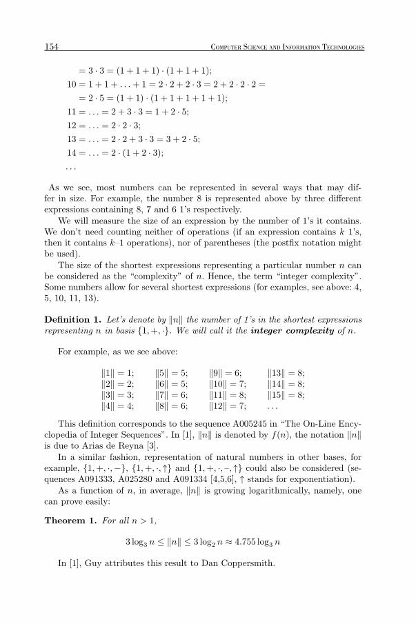
= 3 · 3 = (1 + 1 + 1) · (1 + 1 + 1);
10 = 1 + 1 + . . .+ 1 = 2 · 2 + 2 · 3 = 2 + 2 · 2 · 2 =
= 2 · 5 = (1 + 1) · (1 + 1 + 1 + 1 + 1);
11 = . . . = 2 + 3 · 3 = 1 + 2 · 5;12 = . . . = 2 · 2 · 3;13 = . . . = 2 · 2 + 3 · 3 = 3 + 2 · 5;14 = . . . = 2 · (1 + 2 · 3);. . .
As we see, most numbers can be represented in several ways that may dif-fer in size. For example, the number 8 is represented above by three differentexpressions containing 8, 7 and 6 1’s respectively.
We will measure the size of an expression by the number of 1’s it contains.We don’t need counting neither of operations (if an expression contains k 1’s,then it contains k–1 operations), nor of parentheses (the postfix notation mightbe used).
The size of the shortest expressions representing a particular number n canbe considered as the “complexity” of n. Hence, the term “integer complexity”.Some numbers allow for several shortest expressions (for examples, see above: 4,5, 10, 11, 13).
Definition 1. Let’s denote by ‖n‖ the number of 1’s in the shortest expressionsrepresenting n in basis {1,+, ·}. We will call it the integer complexity of n.
For example, as we see above:
‖1‖ = 1; ‖5‖ = 5; ‖9‖ = 6; ‖13‖ = 8;‖2‖ = 2; ‖6‖ = 5; ‖10‖ = 7; ‖14‖ = 8;‖3‖ = 3; ‖7‖ = 6; ‖11‖ = 8; ‖15‖ = 8;‖4‖ = 4; ‖8‖ = 6; ‖12‖ = 7; . . .
This definition corresponds to the sequence A005245 in “The On-Line Ency-clopedia of Integer Sequences”. In [1], ‖n‖ is denoted by f(n), the notation ‖n‖is due to Arias de Reyna [3].
In a similar fashion, representation of natural numbers in other bases, forexample, {1,+, ·,−}, {1,+, ·, ↑} and {1,+, ·, –, ↑} could also be considered (se-quences A091333, A025280 and A091334 [4,5,6], ↑ stands for exponentiation).
As a function of n, in average, ‖n‖ is growing logarithmically, namely, onecan prove easily:
Theorem 1. For all n > 1,
3 log3 n ≤ ‖n‖ ≤ 3 log2 n ≈ 4.755 log3 n
In [1], Guy attributes this result to Dan Coppersmith.
154 COMPUTER SCIENCE AND INFORMATION TECHNOLOGIES
LURaksti787-datorzinatne.indd 154LURaksti787-datorzinatne.indd 154 23.10.2012 12:02:5823.10.2012 12:02:58

Jānis Iraids, Kaspars Balodis, et al. Integer Complexity: Experimental and Analytical Results
The lower bound of Theorem 1 is reached by infinitely many numbers n,exactly – by the powers of three. For example,
34 = 81 = (1 + 1 + 1) · (1 + 1 + 1) · (1 + 1 + 1) · (1 + 1 + 1),
and, indeed, products of 1 + 1 + 1s is the best way of representing powers ofthree in basis {1,+, ·}:Theorem 2. ‖n‖ = 3 log3 n, if and only if n = 3b for some b ≥ 1. In particular,for all b ≥ 1,
∥∥3b∥∥ = 3b (moreover, the product of 1+1+1’s is shorter than anyother representation of 3b).
Similarly, the product of 1 + 1s seems to be the best way of representingpowers of two in basis {1,+, ·}. For example,
25 = 32 = (1 + 1) · (1 + 1) · (1 + 1) · (1 + 1) · (1 + 1).
Hypothesis 1. For all a ≥ 1, ‖2a‖ = 2a (moreover, the product of 1 + 1’s isshorter than any other representation of 2a).
‖2a‖ = 2a is true for all powers 2a < 1012, i.e. for all a, 0 < a ≤ 39 – asverified by Janis Iraids. We consider proving or disproving of Hypothesis 1 asone of the biggest challenges of number theory.
The upper bound of Theorem 1 doesn’t seem to be exact. As observed by
Rawsthorne [7], the “worst” value of ‖n‖log3 n seems to be ≈ 3.928 (and not 4.755
of Theorem 1), and it is reached only by a single number, namely, by 1439(‖1439‖ = 26):
Hypothesis 2. For all n > 1,
‖n‖ ≤ ‖1439‖log3 1439
log3 n ≈ 3.928 log3 n
Hypothesis 2 is true for all n ≤ 1012 – as verified by Janis Iraids.Thus, we arrive here very soon at the problems that are easy to formulate,
but (it seems) extremely hard to solve. In this paper we represent our attemptsto explore the field by means of experimental mathematics. We managed toprove analytically only a few of the experimental observations.
In Section 2 we explain the basic concepts and their simplest properties. Sec-tion 3 represents our analytical results. Section 4 considers algorithms allowingto calculate the values of ‖n‖. The best of them was used by Janis Iraids to cal-culate ‖n‖ up to n = 1012. In Section 5 we present our experimental observations(several confirmed and refuted hypotheses included).
2 Basic concepts and related work
2.1 The largest and smallest numbers of complexity n
For a given n, there exists only a finite number of expressions of size ≤ n. Hence,
155
LURaksti787-datorzinatne.indd 155LURaksti787-datorzinatne.indd 155 23.10.2012 12:02:5923.10.2012 12:02:59
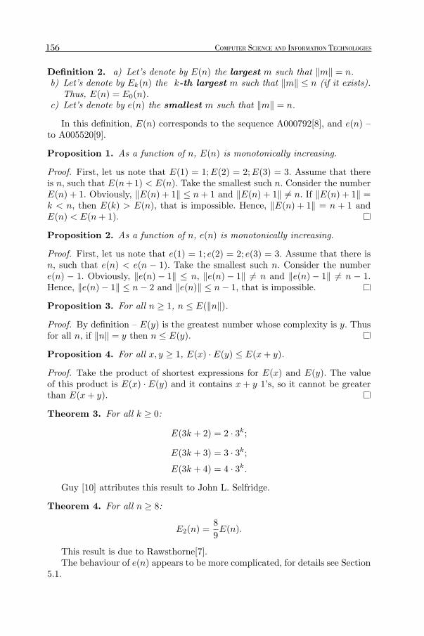
Definition 2. a) Let’s denote by E(n) the largest m such that ‖m‖ = n.b) Let’s denote by Ek(n) the k-th largest m such that ‖m‖ ≤ n (if it exists).
Thus, E(n) = E0(n).c) Let’s denote by e(n) the smallest m such that ‖m‖ = n.
In this definition, E(n) corresponds to the sequence A000792[8], and e(n) –to A005520[9].
Proposition 1. As a function of n, E(n) is monotonically increasing.
Proof. First, let us note that E(1) = 1;E(2) = 2;E(3) = 3. Assume that thereis n, such that E(n+1) < E(n). Take the smallest such n. Consider the numberE(n) + 1. Obviously, ‖E(n) + 1‖ ≤ n+ 1 and ‖E(n) + 1‖ = n. If ‖E(n) + 1‖ =k < n, then E(k) > E(n), that is impossible. Hence, ‖E(n) + 1‖ = n + 1 andE(n) < E(n+ 1).
Proposition 2. As a function of n, e(n) is monotonically increasing.
Proof. First, let us note that e(1) = 1; e(2) = 2; e(3) = 3. Assume that there isn, such that e(n) < e(n − 1). Take the smallest such n. Consider the numbere(n) − 1. Obviously, ‖e(n)− 1‖ ≤ n, ‖e(n)− 1‖ = n and ‖e(n)− 1‖ = n − 1.Hence, ‖e(n)− 1‖ ≤ n− 2 and ‖e(n)‖ ≤ n− 1, that is impossible.
Proposition 3. For all n ≥ 1, n ≤ E(‖n‖).Proof. By definition – E(y) is the greatest number whose complexity is y. Thusfor all n, if ‖n‖ = y then n ≤ E(y).
Proposition 4. For all x, y ≥ 1, E(x) · E(y) ≤ E(x+ y).
Proof. Take the product of shortest expressions for E(x) and E(y). The valueof this product is E(x) · E(y) and it contains x + y 1’s, so it cannot be greaterthan E(x+ y).
Theorem 3. For all k ≥ 0:
E(3k + 2) = 2 · 3k;E(3k + 3) = 3 · 3k;E(3k + 4) = 4 · 3k.
Guy [10] attributes this result to John L. Selfridge.
Theorem 4. For all n ≥ 8:
E2(n) =8
9E(n).
This result is due to Rawsthorne[7].The behaviour of e(n) appears to be more complicated, for details see Section
5.1.
156 COMPUTER SCIENCE AND INFORMATION TECHNOLOGIES
LURaksti787-datorzinatne.indd 156LURaksti787-datorzinatne.indd 156 23.10.2012 12:02:5923.10.2012 12:02:59
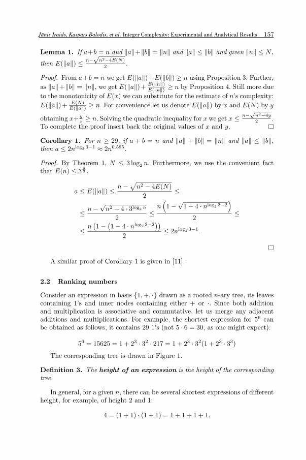
Jānis Iraids, Kaspars Balodis, et al. Integer Complexity: Experimental and Analytical Results
Lemma 1. If a+b = n and ‖a‖+‖b‖ = ‖n‖ and ‖a‖ ≤ ‖b‖ and given ‖n‖ ≤ N ,
then E(‖a‖) ≤ n−√
n2−4E(N)
2 .
Proof. From a+b = n we get E(‖a‖)+E(‖b‖) ≥ n using Proposition 3. Further,
as ‖a‖+‖b‖ = ‖n‖, we get E(‖a‖)+ E(‖n‖)E(‖a‖) ≥ n by Proposition 4. Still more due
to the monotonicity of E(x) we can substitute for the estimate of n’s complexity:
E(‖a‖)+ E(N)E(‖a‖) ≥ n. For convenience let us denote E(‖a‖) by x and E(N) by y
obtaining x+ yx ≥ n. Solving the quadratic inequality for x we get x ≤ n−
√n2−4y
2 .To complete the proof insert back the original values of x and y.
Corollary 1. For n ≥ 29, if a + b = n and ‖a‖ + ‖b‖ = ‖n‖ and ‖a‖ ≤ ‖b‖,then a ≤ 2nlog2 3−1 ≈ 2n0.585.
Proof. By Theorem 1, N ≤ 3 log2 n. Furthermore, we use the convenient factthat E(n) ≤ 3
n3 .
a ≤ E(‖a‖) ≤ n−√n2 − 4E(N)
2≤
≤ n−√n2 − 4 · 3log2 n
2≤
n(1−√
1− 4 · nlog2 3−2)
2≤
≤ n(1− (
1− 4 · nlog2 3−2))
2≤ 2nlog2 3−1.
A similar proof of Corollary 1 is given in [11].
2.2 Ranking numbers
Consider an expression in basis {1,+, ·} drawn as a rooted n-ary tree, its leavescontaining 1’s and inner nodes containing either + or ·. Since both additionand multiplication is associative and commutative, let us merge any adjacentadditions and multiplications. For example, the shortest expression for 56 canbe obtained as follows, it contains 29 1’s (not 5 · 6 = 30, as one might expect):
56 = 15625 = 1 + 23 · 32 · 217 = 1 + 23 · 32(1 + 23 · 33)The corresponding tree is drawn in Figure 1.
Definition 3. The height of an expression is the height of the correspondingtree.
In general, for a given n, there can be several shortest expressions of differentheight, for example, of height 2 and 1:
4 = (1 + 1) · (1 + 1) = 1 + 1 + 1 + 1,
157
LURaksti787-datorzinatne.indd 157LURaksti787-datorzinatne.indd 157 23.10.2012 12:02:5923.10.2012 12:02:59
Fig. 1. The tree of the shortest expression for 56
or of height 4, 3 and 2:
10 = (1+1)·(1+(1+1)·(1+1)) = 1+(1+1+1)·(1+1+1) = (1+1)·(1+1+1+1+1).
We will be interested in classifying the shortest expressions by introducing ex-pression height as another complexity measure of positive integers:
Definition 4. rank(n) – the rank of a number n – is defined as the minimumheight among the shortest expressions representing n.
Examples:
∗ the only number of rank 0 is 1;∗ the only numbers of rank 1 are: 2, 3, 4, 5;∗ numbers of rank 2: 6, 8, 9, 10, 12, 15, ...; see Hypothesis 5 below;∗ rank(7) = rank(11) = rank(13) = 3;∗ rank(14) = 4.
For n ≤ 109, max rank(n) = 19 and max ‖n‖ = 67. For other observations –see Section 5.4.
Obviously rank(n) = 2 for infinitely many numbers n. Namely, for all thepowers of 3.
There are infinitely many numbers n having rank(n) = 3 and 4 as well, seeTheorems 6 and 7 below.
Hypothesis 3. For any r ≥ 2 there exists an infinite amount of numbers havingrank r.
This hypothesis implies
Hypothesis 4. As a function of n, rank(n) is unlimited.
158 COMPUTER SCIENCE AND INFORMATION TECHNOLOGIES
LURaksti787-datorzinatne.indd 158LURaksti787-datorzinatne.indd 158 23.10.2012 12:02:5923.10.2012 12:02:59

Jānis Iraids, Kaspars Balodis, et al. Integer Complexity: Experimental and Analytical Results
Definition 5. Let’s denote by r(n) the smallest m such that rank(m) = n.
The values of r(n) up to n=19 are represented in Table 4.Now, let’s try exploring more closely the numbers of rank 2.
Lemma 2. For n > 1, the shortest expression of height ≤ 2 representing n, isobtained from the prime decomposition p1 · . . . ·pk of n as (1+ . . .+1) · (1+ . . .+1) · . . . · (1 + . . .+ 1).
The number of 1’s in this expression, i.e. p1 + . . . + pk, is called also theinteger logarithm of n (see also the sequence A001414[12]).
Theorem 5. If rank(n) = 2, then n = 2a3b5c for some a, b, c with a+b+c > 1and c < 6.
Proof. (Janis Iraids, Rihards Opmanis) If n ≤ 5, then rank(n) ≤ 1. If n isdivisible by a prime p > 5, then (since ‖p‖ < p) one can convert the expressionof Lemma 2 into a shorter expression representing n. Hence, if rank(n) = 2,then n = 2a3b5c for some a, b, c with a + b + c > 1. But
∥∥56∥∥ < 5 · 6 with theshortest expression being of height 5, as seen in Figure 1. Hence, if n is divisibleby 56, then, again, one can convert the expression of Lemma 2 into a shorterexpression representing n.
Theorem 6. For any k > 0, rank(34k + 1) = 3. Hence, there are infinitelymany numbers n having rank(n) = 3.
Proof. (Janis Iraids) For any k > 0, rank(34k + 1) ≤ 3. These numbers are notdivisible by 3, 4 and 5, hence, they cannot be represented as 2a3b5c. Accordingto Theorem 5, this means that rank(34k + 1) > 2.
Theorem 7. For any k > 0, rank(34k(34k + 1)) = 4. Hence, there are infinitelymany numbers n having rank(n) = 4.
Proof. (Rihards Opmanis) Let us denote N = 34k(34k + 1). For any k > 0,rank(N) ≤ 4, and ‖N‖ ≤ 3 · 8k + 1.
Since N is not divisible by 3, 4 and 5, it cannot be represented as 2a3b5c.According to Theorem 5, this means that rank(N) > 2.
It remains to prove that rank(N) = 3. If rank(N) = 3, then the best ex-pression of N has the form N = X + Y . We will prove that if ‖X‖ ≤ ‖Y ‖ and‖X‖+ ‖Y ‖ ≤ 3 · 8k + 1, then X + Y < N .
Let us recall that
E(3n− 1) = 2 · 3n−1;E(3n) = 3n;E(3n+ 1) = 4 · 3n−1;E(3n+ 1) = 2 · 3n.
Case 1: m ≥ 1; ‖X‖ = 3m; 3m ≤ ‖Y ‖ ≤ 3 · 8k + 1− 3m = 3(8k −m) + 1.Hence, 6m ≤ 3 · 8k + 1;m ≤ 4k; 8k −m ≥ 4k, and
X ≤ E(3m) = 3m;Y ≤ E(3(8k−m)+1) = 4·38k−m−1;X+Y ≤ 3m+4·38k−m−1.
159
LURaksti787-datorzinatne.indd 159LURaksti787-datorzinatne.indd 159 23.10.2012 12:02:5923.10.2012 12:02:59

Consider the items of the latter sum, their product is constant, hence, the sumwill be maximal at m = 1 or m = 4k, i.e. the maximum will be either
3 + 4 · 38k−2 = 38k(31−8k +4
9) < 38k(1 + 3−4k) = N,
or34k + 4 · 34k−1 = 38k(3−4k + 4 · 3−1−4k) < N.
Case 2: m ≥ 0; ‖X‖ = 3m+1; 3m+1 ≤ ‖Y ‖ ≤ 3·8k+1−3m−1 = 3(8k−m).Hence, 6m+ 1 ≤ 3 · 8k;m ≤ 4k − 1; 8k −m ≥ 4k + 1.
If m = 0:
X = 1;Y ≤ E(3 · 8k) = 38k;X + Y ≤ 1 + 38k < N.
If m > 0:
X ≤ E(3m+1) ≤ 4·3m−1;Y ≤ E(3(8k−m)) = 38k−m;X+Y ≤ 4·3m−1+38k−m.
Consider the items of the latter sum, their product is constant, hence, the sumwill be maximal at m = 1 or m = 4k − 1, i.e. the maximum will be either
4 + 38k−1 = 38k(4 · 3−8k +1
3) < 38k(1 + 3−4k) = N,
or4 · 34k−2 + 34k+1 = 38k(4 · 3−4k−2 + 31−4k) < N.
Case 3: m ≥ 0; ‖X‖ = 3m + 2; 3m + 2 ≤ ‖Y ‖ ≤ 3 · 8k + 1 − 3m − 2 =3(8k −m)− 1. Hence, 6m+ 3 ≤ 3 · 8k;m ≤ 4k − 1; 8k −m ≥ 4k + 1.
If m = 0:
X = 2;Y ≤ E(3 ·8k−1) = 2 ·38k−1;X+Y ≤ 2+38k−1 = 38k(2 ·3−8k+1
3) < N.
If m > 0:
X ≤ E(3m+2) ≤ 2·3m;Y ≤ E(3(8k−m)−1) = 2·38k−m−1;X+Y ≤ 2·3m+2·38k−m−1.
Consider the items of the latter sum, their product is constant, hence, the sumwill be maximal at m = 1 or m = 4k − 1, i.e. the maximum will be either
6 + 2 · 38k−2 = 38k(6 · 3−8k +2
9) < 38k(1 + 3−4k) = N,
or2 · 34k−1 + 2 · 34k = 38k(2 · 3−4k−1 + 2 · 3−4k) < N.
Hypothesis 5. All and only numbers of rank 2 are the numbers 2a3b5c > 5with c < 6. Or, extending Hypothesis 1:∥∥2a3b5c∥∥ = 2a+ 3b+ 5c
for all a, b, c with a+ b+ c > 0 and c < 6 (moreover, the product of 1 + ...+ 1sis shorter than any other representation of 2a3b5c).
As verified by Janis Iraids,∥∥2a3b5c∥∥ = 2a+3b+5c is true for all 2a3b5c ≤ 1012
with a+ b+ c > 0 and c < 6.For c = 0, Hypothesis 5 appears in [7].
160 COMPUTER SCIENCE AND INFORMATION TECHNOLOGIES
LURaksti787-datorzinatne.indd 160LURaksti787-datorzinatne.indd 160 23.10.2012 12:02:5923.10.2012 12:02:59

Jānis Iraids, Kaspars Balodis, et al. Integer Complexity: Experimental and Analytical Results
2.3 Logarithmic complexity
Because of Theorem 1, the values of ‖n‖log3 n are located within the segment
[3, 4.755]. Hence, the
Definition 6. The logarithmic complexity of n > 1 is defined as
‖n‖log =‖n‖log3 n
.
For example, ‖2‖log = ‖2‖log3 2 ≈ 3.1699.
Hypothesis 6. It would follow from Hypothesis 5, that the values of ‖n‖log aredense across the segment [3, ‖2‖log], i.e. no subsegment of it is free from thevalues of ‖n‖log.
Proof. According to Hypothesis 5,∥∥2a3b∥∥ = 2a + 3b, for all a + b > 0. Hence,
by choosing a and b appropriately, one can locate the value of∥∥2a3b∥∥
logwithin
any given subsegment of [3, ‖2‖log].As observed by Martins Opmanis (and confirmed by Janis Iraids for all the
numbers ≤ 1012), it seems, the largest values of ‖n‖log are taken by single num-bers, see Table 1. The lists in braces represent Cunningham chains of primes[13].
Table 1: Largest values of ‖n‖log
n ‖n‖ ≈ ‖n‖log rank(n) Other properties
1439 26 3.928 9 e(26), r(9), {89, 179, 359, 719, 1439, 2879}23 11 3.854 5 e(11), r(5), {2, 5, 11, 23, 47}719 23 3.841 7 e(23), {89, 179, 359, 719, 1439, 2879}179 18 3.812 7 e(18), r(7), {89, 179, 359, 719, 1439, 2879}4283 29 3.809 7 e(29), {2141, 4283}1438 25 3.777 8 e(25), 2× 71959 14 3.772 5 e(14), {29, 59}
6299 30 3.767 7 e(30), prime15287 33 3.763 9 e(33), {3821, 7643, 15287}
107 16 3.762 5 e(16), {53, 107}347 20 3.756 7 e(20), {173, 347}1499 25 3.756 7 prime467 21 3.754 5 e(21), {233, 467}
11807 32 3.749 7 e(32), {5903, 11807}263 19 3.746 5 e(19), {131, 263}
21599 34 3.743 7 e(34), {2699, 5399, 10799, 21599}
161
LURaksti787-datorzinatne.indd 161LURaksti787-datorzinatne.indd 161 23.10.2012 12:02:5923.10.2012 12:02:59
The values of ‖n‖log become (and, it seems, stay) less than 3.60 approxi-
mately at n = 2 · 109.Let’s consider the subsegments [C,D], C < D of the segment [3, 4.755] that
do not contain the values of ‖n‖log at all. Of course, according to Hypothesis 6,then C > ‖2‖log. Let’s denote by C1 the infimum of these numbers. I.e. C1 is thepoint separating the area where the values of ‖n‖log are dense, from the area,where these values are not dense.
Hypothesis 7. It would follow from Hypothesis 5, that C1 ≥ ‖2‖log.On the other hand, for some numbers C, ‖n‖log > C only for finitely many
values of n. Let’s denote by C2 the infimum of these numbers. This is also knownas lim sup
n→∞‖n‖log. I.e. C2 is the point separating the area where the values of
‖n‖log are ”absolutely sparse”, from the area, where these values are not sparse.Of course, C1 ≤ C2. Hence,
Hypothesis 8. It would follow from Hypothesis 5, that C2 ≥ ‖2‖log.More about the possible value of C2 – in Section 5.1.
3 Analytical results
3.1 Complexity of 2n − 1
For the sake of brevity let us introduce A(n) = ‖2n − 1‖ − 2n and B(n) =‖2n + 1‖ − 2n. We can then establish the following facts.
Theorem 8. For n ≥ 1,
a) A(2n) ≤ A(n) +B(n);b) A(3n) ≤ A(n) +B(n) + 1;c) A(n+ 1) ≤ A(n) + 1.
Proof. We shall provide the expressions that will result in these upper bounds.
a) 22n−1 = (2n−1)(2n+1). If we take the complexity of both sides and subtract4n we get:
A(2n) =∥∥22n − 1
∥∥− 4n ≤ ‖2n − 1‖ − 2n+ ‖2n + 1‖ − 2n = A(n) +B(n).
b) 23n − 1 = (2n − 1)((2n + 1)2n + 1). Similarly, we get
A(3n) =∥∥23n − 1
∥∥− 6n ≤≤ ‖2n − 1‖ − 2n+ ‖2n + 1‖ − 2n+ ‖2n‖ − 2n+ 1 ≤≤ A(n) +B(n) + 1.
162 COMPUTER SCIENCE AND INFORMATION TECHNOLOGIES
LURaksti787-datorzinatne.indd 162LURaksti787-datorzinatne.indd 162 23.10.2012 12:02:5923.10.2012 12:02:59

Jānis Iraids, Kaspars Balodis, et al. Integer Complexity: Experimental and Analytical Results
c) 2n+1 − 1 = (2n − 1) · 2 + 1. Once again we have
A(n+ 1) =∥∥2n+1 − 1
∥∥− 2n− 2 ≤ ‖2n − 1‖ − 2n+ 2− 2 + 1 = A(n) + 1.
This method can be extended for numbers other than 2, but then it yieldssignificantly less interesting results because of the very inefficient “n + 1” step.
Corollary 2. (Kaspars Balodis) If n > 1, then
‖2n − 1‖ ≤ 2n+ �log2 n�+H(n)− 3,
where H(n) is the number of 1’s in the binary representation of n, i.e., H(n) isthe Hamming weight of n in binary.
Proof. Using the above theorem we can obtain an upper bound of A(n), settingB(n) = 1 and A(1) = A(2) = −1 and ignoring the rule b) altogether. We willuse rule c) per every 1 in the binary representation of n except the leftmostdigit, in total, H(n) − 1 times. We will use rule a) per every digit, except thetwo leftmost digits, in total, �log2 n� − 1 times. In this way we will reduce n to2 at which point A(n) = −1 having “paid” 1 for each application of any of therules a) and c). To sum up:
A(n) ≤ H(n)− 1 + �log2 n� − 1 + (−1).
Corollary 3. If n > 1, then ‖2n − 1‖ ≤ 2n+ 2 �log2 n� − 2.
3.2 Connection of rank and defect
Definition 7. (Harry Altman, Joshua Zelinsky, see [14]) The defect of anumber n is
d(n)def= ‖n‖ − 3 · log3 n.
Proposition 5. (Janis Iraids)
d(n) ≥⌊rank(n)− 1
2
⌋(1 + 3 log3
6
7
).
Proof. We will prove this by induction on the rank. First of all, for all n havingrank(n) < 3 the proposition is true trivially since
⌊rank(n)− 1
2
⌋(1 + 3 log3
6
7
)≤ 0.
Now assuming that it is true for all n having rank(n) < r. Suppose r is an evennumber, then we again trivially have⌊
r − 1
2
⌋(1 + 3 log3
6
7
)=
⌊r − 2
2
⌋(1 + 3 log3
6
7
).
163
LURaksti787-datorzinatne.indd 163LURaksti787-datorzinatne.indd 163 23.10.2012 12:02:5923.10.2012 12:02:59
If on the other hand, r is an odd number greater than 2, then the shortestexpression for n has height at least 3, addition being the outermost operation.Now write n as a sum of numbers of even rank lower than r and order them innon-increasing fashion. This can be done since the numbers of odd rank can besplit down further merging them with the n’s outermost addition.
n =k∑
i=1
ai, rank(a1) ≥ rank(a2) ≥ · · · ≥ rank(ak).
Note that rank(a1) = r − 1 and k ≥ 2. For defects, we have
d(n) =
k∑i=1
d(ai) + 3 log3
∏ki=1 ai∑ki=1 ai
.
Following the induction the defect of a1 is at least r−32
(1 + 3 log3
67
). If
rank(ak) ≥ 2 and so all ai must necessarily be at least 6. The expression
3 log3
∏ki=1 ai∑ki=1 ai
is minimised when k = 2 and a1 = a2 = 6 producing a minimum of
3. However, if there are l numbers of rank 0: rank(ak−l+1) = . . . = rank(ak) = 0
then d(ak−l+1) = . . . = d(ak) = 1 and∑k
i=k−l+1 d(ai) + 3 log3
∏ki=1 ai∑ki=1 ai
is min-
imised at l = 1, a1 = 6 and a2 = 1 giving the 1 + 3 log367 . Consequently,
d(n) ≥ r − 3
2
(1 + 3 log3
6
7
)+min
(3, 1 + 3 log3
6
7
)=
=r − 1
2
(1 + 3 log3
6
7
).
4 Algorithms for computing the complexity of a number
The purpose of this chapter is to describe several algorithms for computing ‖n‖.This is useful for both exploring the behaviour of the complexity and as well asa tool for verifying whether some hypotheses about the value of ‖n‖ hold forlarge n.
It appears that computing the complexity of number n is a relatively difficulttask. At the time of writing we are unaware of any algorithm that provably worksfaster than O(nlog2 3−1). Yet there exists an algorithm, that in practice runs inapproximately Θ (n log n) time.
The first and simplest algorithm is essentially as follows: evaluate all thepossible expressions of {1,+, ·} with increasing number of 1’s until an expressiongiving n is found. We can do so taking as basis the postfix notation, also knownas Reverse Polish notation. Note, that in the postfix notation the first (leftmost)symbol will always be 1.
The possible expression generator will use three main rules to reduce thenumber of generated expressions with equal values:
164 COMPUTER SCIENCE AND INFORMATION TECHNOLOGIES
LURaksti787-datorzinatne.indd 164LURaksti787-datorzinatne.indd 164 23.10.2012 12:03:0023.10.2012 12:03:00

Jānis Iraids, Kaspars Balodis, et al. Integer Complexity: Experimental and Analytical Results
a) After 1 only + or 1 can follow.b) After + only · or 1 can follow.c) After · only + or 1 can follow.
For each total number of 1’s x in the expression excluding the leading onewe can count the number of distinct expressions as 4x – postfix notation of anexpression with x+1 1’s contains 2x+1 symbols and for each symbol there aretwo possible symbols that can follow. Assuming, that evaluation of the expressiontakes roughly x time, the overall time complexity can be estimated as O (4x).Thus the overall running time of the algorithm will be O
(4‖n‖
), which taking
into account ‖n‖ ≤ 3 log2 n will yield O(n6).
However, the expression generating algorithm can be improved by eliminatingsimilar expressions of the same number. For instance, 6 can be represented as
∗ (1 + 1) · (1 + 1 + 1) – postfix notation 11 + 11 + 1 + · or∗ (1 + 1 + 1) · (1 + 1) – postfix notation 11 + 1 + 11 + ·.
Since multiplication is associative, we can omit one of these representationsrestricting that the first multiplier has to be smaller or equal to the secondmultiplier. The same principle applies to additions.
The second algorithm uses the idea of sieving. We will use an array f [1..n]of integer values where the complexity of the number n will be stored as f [n]. Be-fore the main routine starts, precalculate the values of E(n) in an array E[1..m].
for i = 1 to n dof [i] ← i
updated ← Trueheight ← 2while updated do
updated ← Falseif height ≡ 1 (mod 2) then
for i = 2 to n do
a ← n−√
n2−4E[f [n]]
2for j = 1 to a do
if f [i] > f [j] + f [i− j] thenf [i] ← f [j] + f [i− j]
a ← n−√
n2−4E[f [n]]
2updated ← True
elsefor i = 2 to �√n� do
j ← i+ ik ← 2while j ≤ n do
if f [j] > f [k] + f [i] thenf [j] ← f [k] + f [i]updated ← True
j ← j + i
165
LURaksti787-datorzinatne.indd 165LURaksti787-datorzinatne.indd 165 23.10.2012 12:03:0023.10.2012 12:03:00
k ← k + 1
height ← height+ 1
If the array f is initialized as shown each pass will only update the complex-ity of numbers that have rank(n) ≥ height. As a consequence, this algorithmproduces the rank of a number; the rank can be stored if necessary. Note thatthe array f could be initialized with the upper bound provided by Theorem 1because at no point would f [i] be smaller than ‖i‖ and yet exceed the value atthe corresponding point in unmodified algorithm. To further reduce the runningtime, one can use a bootstrapping step where numbers that could potentiallybe used as the smallest of two addends are computed. These are exactly thenumbers that cannot be represented best as sums.
While the second algorithm is as fast as any we know, it uses a linear amountof memory – the array where the complexity values are stored. For n > 1011 thecalculation thus becomes unfeasible. We used this algorithm to calculate ‖n‖and rank(n) up to n = 1.5 · 109.
The third and final algorithm – the one we used for calculating ‖n‖ for nup to 1012 – is conceptually very simple: for every natural number compute thecomplexity by definition and store for subsequent steps.
‖1‖ = 1 (1)
‖n‖ = mina+b=n∨a·b=n
{‖a‖+ ‖b‖} (2)
The techniques used are identical to what Fuller [15] describes in the comments ofhis program. For factorisation we used an approach similar to the one describedin [16]. The core idea is to maintain a priority queue of the so called eliminators– at any point n for each prime the priority is the smallest integer multiple thatis no less than n.
5 Experimental results
5.1 e(n) – the least number of complexity n
Function e(n) corresponds to the sequence A005520 [9]. Our observations up ton = 89 are represented in Table 2.
Hypothesis 9. e(n) is prime for all n, except n ∈ {1, 4, 7, 11, 25}.Observation 1. For k ≤ 3, the number e(n)−k
k+1 is prime for almost all n.
If, for k = 1, Observation 1 holds for an infinite number of values of n, itwould imply that there is an infinite number of Sophie Germain primes –these are defined as integers p such that p and 2p+ 1 are both primes.
Moreover, it seems that the sequence of e(n) contains primes which are theend numbers of increasingly long Cunningham chains. Cunningham chain(CC) of length k is defined as a sequence of k primes {p1, p2, ..., pk} such thatpi+1 = 2 · pi + 1, 1 ≤ i < k [13]. In particular,
166 COMPUTER SCIENCE AND INFORMATION TECHNOLOGIES
LURaksti787-datorzinatne.indd 166LURaksti787-datorzinatne.indd 166 23.10.2012 12:03:0023.10.2012 12:03:00
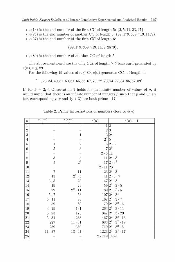
Jānis Iraids, Kaspars Balodis, et al. Integer Complexity: Experimental and Analytical Results
∗ e(13) is the end number of the first CC of length 5: {2, 5, 11, 23, 47};∗ e(26) is the end number of another CC of length 5: {89, 179, 359, 719, 1439};∗ e(27) is the end number of the first CC of length 6:
{89, 179, 359, 719, 1439, 2879};
∗ e(80) is the end number of another CC of length 5.
The above-mentioned are the only CCs of length ≥ 5 backward-generated bye(n), n ≤ 89.
For the following 19 values of n ≤ 89, e(n) generates CCs of length 4:
{11, 23, 34, 49, 51, 60, 61, 65, 66, 67, 70, 72, 73, 74, 77, 84, 86, 87, 89}.
If, for k = 2; 3, Observation 1 holds for an infinite number of values of n, itwould imply that there is an infinite number of integers p such that p and 3p+2(or, correspondingly, p and 4p+ 3) are both primes [17].
Table 2: Prime factorizations of numbers close to e(n)
n e(n)−23
e(n)−12 e(n) e(n) + 1
1 – – 1 22 – – 2 33 – 1 3 22
4 – – 22 55 1 2 5 2 · 36 5 3 7 23
7 – – 2 · 5 118 3 5 11 22 · 39 5 23 17 2 · 3210 – – 2 · 11 2311 7 11 23 23 · 312 13 22 · 5 41 2 · 3 · 713 3 · 5 23 47 24 · 314 19 29 59 22 · 3 · 515 29 22 · 11 89 2 · 32 · 516 5 · 7 53 107 22 · 3317 5 · 11 83 167 23 · 3 · 718 59 89 179 22 · 32 · 519 3 · 29 131 263 23 · 3 · 1120 5 · 23 173 347 22 · 3 · 2921 5 · 31 233 467 22 · 32 · 1322 227 11 · 31 683 22 · 32 · 1923 239 359 719 24 · 32 · 524 11 · 37 13 · 47 1223 23 · 32 · 1725 – – 2 · 719 1439
167
LURaksti787-datorzinatne.indd 167LURaksti787-datorzinatne.indd 167 23.10.2012 12:03:0023.10.2012 12:03:00

26 479 719 1439 25 · 32 · 527 7 · 137 1439 2879 26 · 32 · 528 5 · 251 7 · 269 3767 23 · 3 · 15729 1427 2141 4283 22 · 32 · 7 · 1730 2099 47 · 67 6299 22 · 32 · 52 · 731 3359 5039 10079 25 · 32 · 5 · 732 5 · 787 5903 11807 25 · 32 · 4133 5 · 1019 7643 15287 23 · 3 · 72 · 1334 23 · 313 10799 21599 25 · 33 · 5235 3 · 3733 107 · 157 33599 26 · 3 · 52 · 736 5 · 23 · 131 2 · 11299 45197 2 · 36 · 3137 18679 28019 56039 23 · 3 · 5 · 46738 5 · 5443 40823 81647 24 · 36 · 739 32999 49499 98999 23 · 32 · 53 · 1140 54419 81629 163259 22 · 32 · 5 · 90741 53 · 1283 101999 203999 25 · 3 · 53 · 1742 80627 120941 241883 22 · 32 · 671943 5 · 24763 185723 371447 23 · 32 · 7 · 11 · 6744 180179 270269 540539 22 · 33 · 5 · 7 · 11 · 1345 196799 295199 590399 26 · 32 · 52 · 4146 302399 453599 907199 26 · 34 · 52 · 747 173 · 2083 540539 1 081 079 23 · 33 · 5 · 7 · 11 · 1348 617039 925559 1 851 119 24 · 33 · 5 · 85749 680399 1 020 599 2 041 199 24 · 36 · 52 · 750 1 081 079 1 621 619 3 243 239 23 · 34 · 5 · 7 · 11 · 1351 1 280 159 1 920 239 3 840 479 25 · 33 · 5 · 7 · 12752 2 187 359 3 281 039 6 562 079 25 · 33 · 5 · 72 · 3153 2 735 519 4 103 279 8 206 559 25 · 32 · 5 · 41 · 13954 3 898 919 5 848 379 11 696 759 23 · 32 · 5 · 3249155 4 882 919 7 324 379 14 648 759 23 · 32 · 5 · 7 · 581356 13 · 59 · 9697 11 156 399 22 312 799 25 · 33 · 52 · 103357 9 164 959 13 747 439 27 494 879 25 · 3 · 5 · 73 · 16758 13 915 439 20 873 159 41 746 319 24 · 33 · 5 · 7 · 11 · 25159 17 417 399 26 126 099 52 252 199 23 · 32 · 52 · 7 · 11 · 13 · 2960 26 110 559 39 165 839 78 331 679 25 · 32 · 5 · 7 · 19 · 40961 36 202 319 54 303 479 108 606 959 24 · 33 · 5 · 7 · 11 · 65362 6577 · 7247 71 495 279 142 990 559 25 · 32 · 5 · 109 · 91163 67 699 439 101 549 159 203 098 319 24 · 33 · 5 · 17 · 553164 91 328 639 136 992 959 273 985 919 27 · 32 · 5 · 13 · 365965 127 340 639 191 010 959 382 021 919 25 · 34 · 5 · 7 · 421166 165 145 679 247 718 519 495 437 039 24 · 33 · 5 · 72 · 31 · 15167 227 109 119 340 663 679 681 327 359 28 · 32 · 5 · 72 · 17 · 7168 335 430 119 503 145 179 1 006 290 359 23 · 32 · 5 · 601 · 465169 468 798 119 703 197 179 1 406 394 359 23 · 33 · 5 · 7 · 17 · 31 · 35370 619 264 799 928 897 199 1 857 794 399 25 · 33 · 52 · 7 · 11 · 1117
168 COMPUTER SCIENCE AND INFORMATION TECHNOLOGIES
LURaksti787-datorzinatne.indd 168LURaksti787-datorzinatne.indd 168 23.10.2012 12:03:0023.10.2012 12:03:00

Jānis Iraids, Kaspars Balodis, et al. Integer Complexity: Experimental and Analytical Results
71 909 474 719 1 364 212 079 2 728 424 159 25 · 32 · 5 · 7 · 112 · 223772 1 247 732 639 1 871 598 959 3 743 197 919 25 · 34 · 5 · 7 · 113 · 3173 40499 · 41221 2 504 113 919 5 008 227 839 29 · 33 · 5 · 7 · 11 · 94174 2 290 896 719 3 436 345 079 6 872 690 159 24 · 33 · 5 · 7 · 45454375 3 279 830 399 7643 · 643693 9 839 491 199 27 · 34 · 52 · 7 · 11 · 17 · 2976 4 495 159 679 6 742 739 519 13 485 479 039 27 · 32 · 5 · 113 · 175977 5 574 925 439 8 362 388 159 16 724 776 319 27 · 38 · 5 · 7 · 56978 8 226 486 239 12 339 729 359 24 679 458 719 25 · 32 · 5 · 7 · 19 · 12886179 11 841 566 159 17 762 349 239 35 524 698 479 24 · 32 · 5 · 4933985980 14 737 208 639 22 105 812 959 44 211 625 919 26 · 32 · 5 · 72 · 11 · 19 · 149981 20 797 230 719 31 195 846 079 62 391 692 159 27 · 32 · 5 · 72 · 22105982 31 251 071 039 46 876 606 559 93 753 213 119 26 · 32 · 5 · 72 · 61 · 1089183 40 517 305 919 60 775 958 879 121 551 917 759 26 · 34 · 5 · 7 · 13 · 29 · 177784 54 513 320 399 81 769 980 599 163 539 961 199 24 · 33 · 52 · 7 · 11 · 19665785 83 528 413 919 125 292 620 879 250 585 241 759 25 · 34 · 5 · 7 · 276218386 106 809 776 639 160 214 664 959 320 429 329 919 29 · 33 · 5 · 72 · 37 · 255787 141 615 840 239 212 423 760 359 424 847 520 719 24 · 34 · 5 · 7 · 936612788 210 123 688 319 315 185 532 479 630 371 064 959 27 · 33 · 5 · 7 · 13 · 17 · 2358189 290 857 880 879 436 286 821 319 872 573 642 639 24 · 33 · 5 · 73 · 19 · 61987
The behaviour of e(n) provides some evidence that the logarithmic complexityof n does not tend to 3, and even that the constant C2 = lim sup
n→∞‖n‖log is greater
than ‖2‖log. It is useful to note the following fact:
Proposition 6.
C2 = lim supn→∞
‖n‖log = lim supn→∞
‖e(n)‖log
Proof. Since ‖e(n)‖log is a subsequence of ‖n‖log the ≥ follows obviously.The ≤ is proven from the contrary. Assume that there exists an infinite list of
numbers {xi}, that only have a finite number of elements from sequence e(n) oflogarithmic complexity ≥ mini{‖xi‖log}. Furthermore, there is an infinite sub-sequence {yi} of {xi}’s such that the complexity of numbers strongly increases.But any number of this sequence has a corresponding number in e(n), namelye(‖yi‖) that has greater or equal logarithmic complexity.
Alternatively, on the axis of logarithmic complexity, e(n) yields the rightmostpoint of numbers of complexity n.
Hypothesis 10. The limit limn→∞ ‖e(n)‖log exists and
limn→∞ ‖e(n)‖log = lim sup
n→∞‖e(n)‖log
As one can see in Figures 2 and 3:
169
LURaksti787-datorzinatne.indd 169LURaksti787-datorzinatne.indd 169 23.10.2012 12:03:0023.10.2012 12:03:00

0
5
10
15
20
25
0 10 20 30 40 50 60 70 80 90
n
log3 e(n)
Hypothesized asymptote (0.297 · n− 1.55)
Fig. 2. Values of log3 e(n) compared with hypothesized asymptote
0
0.2
0.4
0.6
0.8
1
1.2
1.4
1.6
1.8
0 10 20 30 40 50 60 70 80 90
n
residuals (log3 e(n)− (0.297 · n− 1.55))
Fig. 3. Residuals of the asymptote
170 COMPUTER SCIENCE AND INFORMATION TECHNOLOGIES
LURaksti787-datorzinatne.indd 170LURaksti787-datorzinatne.indd 170 23.10.2012 12:03:0023.10.2012 12:03:00

Jānis Iraids, Kaspars Balodis, et al. Integer Complexity: Experimental and Analytical Results
Hypothesis 11. log3 e(n) behaves almost linearly, namely,
log3 e(n) ≈ 0.297n− 1.55.
Hence,
‖e(n)‖log =n
log3 e(n)≈ 3.37 +
5.2
0.297n− 1.55,
and limn→∞ ‖e(n)‖log ≈ 3.37.
Lemma 3. For all n > 1:
‖n‖log ≤ ‖e(‖n‖)‖log .Proof. Obviously, ‖n‖ = ‖e(‖n‖)‖, and n ≥ e(‖n‖). Hence, log3 n ≥ log3 e(‖n‖),and ‖n‖log ≤ ‖e(‖n‖)‖log.
Thus, if ε > 0, then, it seems, ‖n‖log > 3.37 + ε can be true only for finitelymany values of n. Thus, in terms of Section 2.3:
Hypothesis 12. It would follow from Hypothesis 11, that C2 ≤ 3.37 (approxi-mately).
5.2 Structure of shortest expressions
Analyzing the structure of the shortest expressions representing numbers, wehave come to the conclusion that we should not only abandon any attempts toobtain a ”deterministic” method for construction of shortest expressions, andturn to ”nondeterministic” methods. We should abandon also radical attemptsto predict regularities in the structure of shortest expressions.
For example, one might propose the following hypothesis: if p is the smallestprime divisor of n > 1, then
‖n‖ = min (1 + ‖n− 1‖ , ‖p‖+ ‖n/p‖).
For p = n, and p = 2 (with prime n/p) this hypothesis appears in Guy [10]:for any prime p,
‖p‖ = 1 + ‖p− 1‖ ,‖2p‖ = min (1 + ‖2p− 1‖ , 2 + ‖p‖).
Similarly, one could suppose:
‖3p‖ = min (1 + ‖3p− 1‖ , 3 + ‖p‖).
The first hypothesis fails, the smallest counterexample being
p = 353 942 783 = 2 · 3 + (1 + 22 · 32)(2 + 34(1 + 2 · 310)),
171
LURaksti787-datorzinatne.indd 171LURaksti787-datorzinatne.indd 171 23.10.2012 12:03:0023.10.2012 12:03:00
‖p‖ = 63, 1 + ‖p− 1‖ = 64, found by Martin N. Fuller, 2008, see [2].
The second hypothesis fails as well, the smallest counterexample being
2p = 10 278 600 694 = 2 · 3 + (1 + 2 · 32(1 + 24))(1 + 314(1 + 2 · 3)),
‖2p‖ = 72, 1 + ‖2p− 1‖ = 2 + ‖p‖ = 73, found by Janis Iraids, 2010.
By analogy, it seems, the third hypothesis also should fail, but this does nothappen for 3p ≤ 1012.
Thus, when trying to build the shortest expression representing a number,subtraction of 1 and division by primes are not universal candidates for the firstoperation. How about subtraction of other numbers?
Subtractions of 3, 4, 5, 7, 10, 11, 13, etc. include subtraction of 1. Thus, itremains to consider only subtractions of 6, 8, 9, 12, etc.
The first number, for which subtraction of 6 is necessary as the first operation,is the above prime found by Fuller:
353 942 783 = 2 · 3 + (1 + 22 · 32)(2 + 34(1 + 2 · 310)).
Until 1012, there are only 21360 numbers for which subtraction of 6, 8 or 9is necessary as the first operation.
Until 1012, there are exactly 3 numbers for which the first operation must besubtraction of 8:
341 317 451 698 = 2 · prime = 23 + (1 + 24(1 + 2 · 33))(1 + 318);
474 934 483 834 = 2 · 6011 · 39505447 = 23 + (1 + 24)(1 + 23 · 34)(1 + 316);
782 747 233 558 = 2 · prime = 23 + (1 + 24(1 + 2 · 35))(1 + 315(1 + 2 · 3)).
Until 1012, there are 119 numbers for which the first operation must besubtraction of 9, the first three ones being:
16 534 727 299 = 103 · 160531333 = 32 + (1 + 27 · 33)(1 + 314);
68 238 632 999 = prime = 32 + (1 + 1 + 32)(1 + 24 · 34)(1 + 314);
85 619 928 299 = prime = 32 + (1 + 22 · 3)(1 + 24)(1 + 318).
Necessity for subtraction of 12 (or larger addendum) was not detected fornumbers until 1012.
According to Corollary 1, if n ≥ 29 and the shortest expression for n is asum n = a + b, then the smaller addendum a ≤ 2nlog2 3−1 ≈ 2n0.585. However,the above observations show that for n ≤ 1012 the smaller addendum does notexceed 9.
172 COMPUTER SCIENCE AND INFORMATION TECHNOLOGIES
LURaksti787-datorzinatne.indd 172LURaksti787-datorzinatne.indd 172 23.10.2012 12:03:0023.10.2012 12:03:00

Jānis Iraids, Kaspars Balodis, et al. Integer Complexity: Experimental and Analytical Results
5.3 Complexity of 2n + 1 and 2n − 1
Since, it seems, ‖2n‖ = 2n, one can suppose
Hypothesis 13. For all n ≥ 0, except 3 and 9,
‖2n + 1‖ = 2n+ 1.
Hypothesis 13 is true for all 2n + 1 ≤ 1012, i.e. for all n ≤ 39 – as verified byJanis Iraids.
Both exceptions are due to relatively massive divisibility by 3:
23 + 1 = 9 = 2 · 2 · 2 + 1 = 3 · 3;
29 + 1 = 513 = (3 · 3 · 2 + 1) · 3 · 3 · 3.On the other hand, since we do not have subtraction in our expression basis
{1,+, ·}, the numbers 2n − 1 seem to be more complicated than 2n. In Theorem2, an upper bound of ‖2n − 1‖ was proved. In Table 3 this result is comparedwith experimental data for n ≤ 39.
Table 3: Complexity of ‖2n − 1‖
n ‖2n − 1‖ − 2n �log2 n�+H(n)− 3 n ‖2n − 1‖ − 2n �log2 n�+H(n)− 31 −1 − 21 2 42 −1 −1 22 3 43 0 0 23 4 54 0 0 24 2 35 1 1 25 3 46 0 1 26 3 47 1 2 27 2 58 1 1 28 3 49 1 2 29 4 510 2 2 30 3 511 3 3 31 4 612 1 2 32 3 313 2 3 33 4 414 2 3 34 4 415 2 4 35 4 516 2 2 36 2 417 3 3 37 2 518 1 3 38 2 519 2 4 39 3 620 2 3 − − −
Thus, it seems, the upper bound of Theorem 2 is exact for all n = 2k, k > 0:
173
LURaksti787-datorzinatne.indd 173LURaksti787-datorzinatne.indd 173 23.10.2012 12:03:0123.10.2012 12:03:01
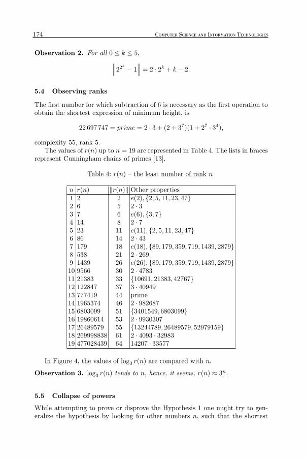
Observation 2. For all 0 ≤ k ≤ 5,
∥∥∥22k − 1∥∥∥ = 2 · 2k + k − 2.
5.4 Observing ranks
The first number for which subtraction of 6 is necessary as the first operation toobtain the shortest expression of minimum height, is
22 697 747 = prime = 2 · 3 + (2 + 37)(1 + 27 · 34),
complexity 55, rank 5.The values of r(n) up to n = 19 are represented in Table 4. The lists in braces
represent Cunningham chains of primes [13].
Table 4: r(n) – the least number of rank n
n r(n) ‖r(n)‖ Other properties1 2 2 e(2), {2, 5, 11, 23, 47}2 6 5 2 · 33 7 6 e(6), {3, 7}4 14 8 2 · 75 23 11 e(11), {2, 5, 11, 23, 47}6 86 14 2 · 437 179 18 e(18), {89, 179, 359, 719, 1439, 2879}8 538 21 2 · 2699 1439 26 e(26), {89, 179, 359, 719, 1439, 2879}10 9566 30 2 · 478311 21383 33 {10691, 21383, 42767}12 122847 37 3 · 4094913 777419 44 prime14 1965374 46 2 · 98268715 6803099 51 {3401549, 6803099}16 19860614 53 2 · 993030717 26489579 55 {13244789, 26489579, 52979159}18 269998838 61 2 · 4093 · 3298319 477028439 64 14207 · 33577
In Figure 4, the values of log3 r(n) are compared with n.
Observation 3. log3 r(n) tends to n, hence, it seems, r(n) ≈ 3n.
5.5 Collapse of powers
While attempting to prove or disprove the Hypothesis 1 one might try to gen-eralize the hypothesis by looking for other numbers n, such that the shortest
174 COMPUTER SCIENCE AND INFORMATION TECHNOLOGIES
LURaksti787-datorzinatne.indd 174LURaksti787-datorzinatne.indd 174 23.10.2012 12:03:0123.10.2012 12:03:01

Jānis Iraids, Kaspars Balodis, et al. Integer Complexity: Experimental and Analytical Results
0
5
10
15
20
0 5 10 15 20
y
n
log3 r(n)
y = n
Fig. 4. Values of log3 r(n) compared with n.
expressions for all the integer powers of n: n2, n3, n4, . . . can be obtained asproducts of shortest expressions for n.
Definition 8. If this property holds, then the number n is called resistant.
Obviously, if n is resistant, then for all k > 0,
∥∥nk∥∥ = k ‖n‖ ;
∥∥nk∥∥log
= ‖n‖log .Currently, only the number 3 is proved to be resistant. According to Hy-
pothesis 1, another resistance candidate is the number 2. Existence of resistantnumbers other than powers of 3 would provide a lower bound on C2:
Proposition 7. If n = 2 or n = 3k is resistant, C2 ≥ ‖n‖log > 3.
Definition 9. If k > 0 is the least number such that∥∥nk
∥∥ < k ‖n‖, let us saythat the number n collapses at k.
For example, the number 5 collapses at 6 (see Section 2.2):
∥∥56∥∥ = 29 < 6 ‖5‖ = 6 · 5 = 30.
175
LURaksti787-datorzinatne.indd 175LURaksti787-datorzinatne.indd 175 23.10.2012 12:03:0123.10.2012 12:03:01

However, it seems, most primes collapse already at 2, for example,
∥∥112∥∥ = 15 < 2 ‖11‖ = 2 · 8 = 16; 112 = 121 = 1 + 23 · 3 · 5.
Of the 168 primes until 103, 120 primes collapse at 2 (71%), 24 – at 3 (14%),3 – at 4 (2%), the remaining 21 do not collapse until 4 (13%), and, currently, 7of them are not known to collapse at all, namely,
2, 3, 109, 163, 433, 487, 577.
More detailed data is represented in Table 5. For numbers whose collapsing powerdoes not exceed 1012 the exact value is given. For some of the other numbers,Juris Cernenoks and Janis Iraids have used specific methods and specific softwareto obtain expressions representing powers nk and containing less than k ‖n‖ 1’s.These numbers n are labeled ≤ k. For example,
7336 = 155104303499468569 =
2 · 32 · (25 · 32 · (2 · 3 + 1)(22 · 3 + 1)(2 · 37 · (2 · 3 + 1)(2 · 33 + 1) + 1) + 1)·(2 · 3 + 1)(2 · 32 + 1)(32 · (2 · 34 + 1) + 1) + 1,
where the expression contains 119 < 120 = 6 · ‖733‖ 1’s.The remaining numbers all collapse at 2 or 3, and their logarithmic com-
plexity exceeds 3.417. It seems, primes having larger logarithmic complexity aremore likely to collapse.
Table 5: Powers in which primes until 1000 collapse, sorted byincreasing logarithmic complexity
p collapses ‖p‖ rank(p) ≈ ‖p‖log3 − 3 1 3.0002 ?(> 39) 2 1 3.170487 ?(> 4) 18 3 3.196163 ?(> 5) 15 3 3.235433 ?(> 4) 18 3 3.257109 ?(> 5) 14 3 3.278811 ≤ 9 20 3 3.280577 ?(> 4) 19 3 3.283769 3 20 3 3.307757 ≤ 6 20 5 3.314541 ≤ 6 19 3 3.317739 ≤ 6 20 5 3.32673 6 13 3 3.329379 ≤ 6 18 5 3.331733 ≤ 6 20 5 3.331271 4 17 3 3.334193 4 16 3 3.340
176 COMPUTER SCIENCE AND INFORMATION TECHNOLOGIES
LURaksti787-datorzinatne.indd 176LURaksti787-datorzinatne.indd 176 23.10.2012 12:03:0123.10.2012 12:03:01

Jānis Iraids, Kaspars Balodis, et al. Integer Complexity: Experimental and Analytical Results
991 ≤ 12 21 5 3.34437 5 11 3 3.347977 2 21 5 3.35119 6 9 3 3.35897 6 14 3 3.362257 ≤ 6 17 3 3.366937 3 21 5 3.372673 3 20 5 3.374919 3 21 5 3.381181 3 16 3 3.381661 3 20 5 3.3847 9 6 3 3.387653 2 20 5 3.390337 3 18 5 3.398641 4 20 3 3.400883 3 21 5 3.401127 2 15 5 3.402881 2 21 5 3.402877 3 21 5 3.405241 3 17 3 3.405631 2 20 5 3.408457 3 19 5 3.408331 3 18 5 3.4085 6 5 1 3.413
Of the 1229 primes until 104, 1030 primes collapse at 2 (84%), 122 – at 3(10%), the remaining 77 do not collapse until 3 (6%).
Of the 78498 primes until 106, 71391 primes collapse at 2 (91%), the remain-ing 7107 do not collapse until 2 (9%), and, currently, only 2722 are not knownto collapse at all (4%).
The following observations are true for primes less than 106.
Observation 4. Almost all primes collapse at 2.
Observation 5. If a prime p does not collapse at all, then ‖p‖log < 3.364. If aprime p collapses, then ‖p‖log > 3.180 > ‖2‖log.
If we turn to composite numbers, we can encounter numbers that collapsebecause one ore more of their prime divisors collapse – even when their initialshortest expression did not directly contain the prime as a multiplier. 34+1 = 82is an example of such a number:
∗ ‖82‖ = 13 and ‖41‖ = 12∗ ∥∥8212∥∥ < 12 · 13, because ∥∥4112∥∥ ≤ 131 < 12 · 11:
4112 =[23 · 32 · (22 + 1) (
37 + 1)
(2 · 34 · (23 · 32 · (2 · 33 + 1
)+ 1
)+ 1
)(2 · 34 · (2 · 39 · (2 · 3 + 1) + 1
)+ 1
)] + 1
177
LURaksti787-datorzinatne.indd 177LURaksti787-datorzinatne.indd 177 23.10.2012 12:03:0123.10.2012 12:03:01

On the other hand, there could possibly be composite numbers that do notcollapse even though some of their prime divisors do. Obviously, a necessarycondition is that the shortest expression for the composite number does notdirectly contain the collapsing prime as a multiplier. One candidate is 35 + 1 =244 = 22 · 61; ‖244‖ = 16 but ‖61‖ = 13. Using a heuristic algorithm JurisCernenoks was able to produce expressions for 61k for k = 7..15. His resultssuggest that 61 does not collapse well enough, i.e., the number of 1’s saved fromcollapsing is less than required to catch up with the expression 244 = 35 + 1.
On a side note, the above mentioned 82 and 244 are interesting because ifthey proved to be resistant, then C2 would exceed ‖2‖log.
6 Conclusions
Trying to explore representing of natural numbers by arithmetical expressionsusing 1’s, addition, multiplication and parentheses, one arrives very soon at theproblems that are easy to formulate, but (it seems) extremely hard to solve.
Consider, for example, the above Hypothesis 1 stating that the best wayof representing of 2n is (1 + 1)(1 + 1).... We consider proving or disproving ofHypothesis 1 as one of the biggest challenges of number theory.
Almost as challenging seems Hypothesis 4 stating that as a function of n,rank(n) is unlimited. Rank is an additional (to ‖n‖) measure of integer com-plexity introduced in this paper.
As another challenge we regard determining of the distribution of the valuesof logarithmic complexity ‖n‖log which are located within the segment [3, 4.755].First, denote by C1 the point separating the area (on the left) where the values of‖n‖log are dense, from the area, where these values are not dense. On the otherhand, on the right, the values of ‖n‖log are ”absolutely sparse”: for most C,‖n‖log > C only for finitely many values of n. Denote by C2 the point separatingthe area (on the right) where the values of ‖n‖log are ”absolutely sparse”, fromthe area, where these values are not sparse. Of course, C1 ≤ C2. Our Hypotheses5 and 11 imply that
3.1699 ≈ ‖2‖log ≤ C1 ≤ C2 ≤ 3.37.
Our main experimental ”device” is the database containing the values of ‖n‖up to n = 1012 calculated by Janis Iraids. The database can be accessed by usingan online calculator page linked from [2].
And finally, our Hypothesis 9 and Observation 1 (if true) imply that there isan infinite number of Sophie Germain primes, and even that there is an infinitenumber of Cunningham chains of length 4 (at least).
178 COMPUTER SCIENCE AND INFORMATION TECHNOLOGIES
LURaksti787-datorzinatne.indd 178LURaksti787-datorzinatne.indd 178 23.10.2012 12:03:0123.10.2012 12:03:01

Jānis Iraids, Kaspars Balodis, et al. Integer Complexity: Experimental and Analytical Results
2. Sloane, N.J.A.: The On-Line Encyclopedia of Integer Sequences. A005245 Com-plexity of n: number of 1’s required to build n using + and ·.
3. Arias de Reyna, J.: Complejidad de los numeros naturales. Gaceta de la RealSociedad Matematica Espanola (2000)
4. Voss, J.: The On-Line Encyclopedia of Integer Sequences. A091333 Number of 1’srequired to build n using +, −, · and parentheses.
5. N. J. A. Sloane, David W. Wilson: The On-Line Encyclopedia of Integer Sequences.A025280 Complexity of n: number of 1’s required to build n using +, · and ↑.
6. Voss, J.: The On-Line Encyclopedia of Integer Sequences. A091334 Number of 1’srequired to build n using +, −, ·, ↑ and parentheses.
7. Rawsthorne, D.A.: How many 1’s are needed? Fibonacci Quarterly (1989)8. Sloane, N.J.A.: The On-Line Encyclopedia of Integer Sequences. A000792 a(n) =
max(n− i)a(i) : i < n; a(0) = 1.9. Sloane, N.J.A.: The On-Line Encyclopedia of Integer Sequences. A005520 Smallest
number of complexity n: smallest number requiring n 1’s to build using + and ·.10. Guy, R.K.: Some suspiciously simple sequences. The American Mathematical
Monthly (1986)11. Srinivas Vivek V., Shankar B. R.: Integer complexity: Breaking the θ(n2) barrier.
World Academy of Science, Engineering and Technology (2008)12. Sloane, N.J.A.: The On-Line Encyclopedia of Integer Sequences. A001414 Integer
log of n: sum of primes dividing n (with repetition).13. Caldwell, C.K.: Cunningham chain14. Harry Altman, Joshua Zelinsky: Numbers with Integer Complexity Close to the
Lower Bound. http://arxiv.org/abs/1207.4841 [Last accessed 15 September2012] (2012)
15. Fuller, M.N.: Program to calculate A005245, A005520, A005421. http://oeis.
org/A005245/a005245.c.txt [Last accessed: 30 December 2011]16. Bennet, T.W.: Prime Generator Algorithm. http://sandbox.mc.edu/~bennet/
cs220/codeex/pgenintro.html [Last accessed 13 January 2012]17. Caldwell, C.K.: Dicksons conjecture. http://primes.utm.edu/glossary/xpage/
DicksonsConjecture.html [Last accessed 13 March 2012]
References
1. Guy, R.K.: F26 Expressing numbers with just ones. In: Unsolved Problems inNumber Theory. Springer Science+Business Media, Inc. (2004)
179
LURaksti787-datorzinatne.indd 179LURaksti787-datorzinatne.indd 179 23.10.2012 12:03:0123.10.2012 12:03:01

LATVIJAS UNIVERSITĀTES RAKSTI787. sējums. Datorzinātne un informācijas tehnoloģijas. 2012
Latvijas Universitātes Akadēmiskais apgādsBaznīcas iela 5, Rīga, LV-1010
Tālr. 67034535
LURaksti787-datorzinatne.indd 180LURaksti787-datorzinatne.indd 180 23.10.2012 12:03:0123.10.2012 12:03:01