a 107 math 2008 lecture notes
TRANSCRIPT
8/6/2019 A 107 Math 2008 Lecture Notes
http://slidepdf.com/reader/full/a-107-math-2008-lecture-notes 1/84
A107 Maths for Aeronautics
Imperial College LondonAutumn Term 2008-2009
Lecture Notes
Stefano Luzzatto
Mathematics department. Imperial College, London SW7 2AZ
http://www.ma.ic.ac.uk/˜luzzatto
These are lecture notes for the first part of the course A107 Mathsfor Aeronautical Engineering Students at Imperial College London.
They include the Basic Maths Course notes prepared by Roy Jacobs in 2005.
The notes together with accompanying problem and solutions sheets
are available for download from the website given above.
Please send any corrections or suggestions to [email protected]
October 8, 2008
8/6/2019 A 107 Math 2008 Lecture Notes
http://slidepdf.com/reader/full/a-107-math-2008-lecture-notes 2/84
2
8/6/2019 A 107 Math 2008 Lecture Notes
http://slidepdf.com/reader/full/a-107-math-2008-lecture-notes 3/84
Contents
1 Basic Maths Course 5
1.1 Arithmetic . . . . . . . . . . . . . . . . . . . . . . . . . . . . . . . . . . . . . . . . 6
1.2 Algebra . . . . . . . . . . . . . . . . . . . . . . . . . . . . . . . . . . . . . . . . . 9
1.3 Combinatorics . . . . . . . . . . . . . . . . . . . . . . . . . . . . . . . . . . . . . . 121.4 Functions and graphs . . . . . . . . . . . . . . . . . . . . . . . . . . . . . . . . . . 14
1.5 Cartesian (or Coordinate) Geometry . . . . . . . . . . . . . . . . . . . . . . . . . . 18
1.6 Trigonometry . . . . . . . . . . . . . . . . . . . . . . . . . . . . . . . . . . . . . . 19
1.7 Vectors and mechanics . . . . . . . . . . . . . . . . . . . . . . . . . . . . . . . . . 22
1.8 Limits of sequences . . . . . . . . . . . . . . . . . . . . . . . . . . . . . . . . . . . 25
2 Derivatives 27
2.1 Definition and basic examples . . . . . . . . . . . . . . . . . . . . . . . . . . . . . 27
2.2 Differentiating combinations of functions . . . . . . . . . . . . . . . . . . . . . . . 29
2.3 Estimating small changes . . . . . . . . . . . . . . . . . . . . . . . . . . . . . . . . 32
2.4 Higher order derivatives . . . . . . . . . . . . . . . . . . . . . . . . . . . . . . . . . 34
3 Integrals 37
3.1 Definitions and basic examples . . . . . . . . . . . . . . . . . . . . . . . . . . . . . 37
3.2 Basic techniques . . . . . . . . . . . . . . . . . . . . . . . . . . . . . . . . . . . . 39
3.3 Recursive relations . . . . . . . . . . . . . . . . . . . . . . . . . . . . . . . . . . . 40
3.4 Rational functions . . . . . . . . . . . . . . . . . . . . . . . . . . . . . . . . . . . . 42
4 Series 47
4.1 Definitions . . . . . . . . . . . . . . . . . . . . . . . . . . . . . . . . . . . . . . . . 47
4.2 Basic test for non-convergence . . . . . . . . . . . . . . . . . . . . . . . . . . . . . 48
4.3 The ratio test . . . . . . . . . . . . . . . . . . . . . . . . . . . . . . . . . . . . . . 494.4 The integral and comparison tests . . . . . . . . . . . . . . . . . . . . . . . . . . . 50
4.5 Power Series . . . . . . . . . . . . . . . . . . . . . . . . . . . . . . . . . . . . . . 52
4.6 Taylor and Maclaurin Series . . . . . . . . . . . . . . . . . . . . . . . . . . . . . . 53
4.7 Taylor’s Theorem . . . . . . . . . . . . . . . . . . . . . . . . . . . . . . . . . . . . 55
5 Limits 59
5.1 Definition and key properties . . . . . . . . . . . . . . . . . . . . . . . . . . . . . . 59
5.2 Basic examples . . . . . . . . . . . . . . . . . . . . . . . . . . . . . . . . . . . . . 59
5.3 Counterexamples . . . . . . . . . . . . . . . . . . . . . . . . . . . . . . . . . . . . 60
5.4 Techniques for calculating limits . . . . . . . . . . . . . . . . . . . . . . . . . . . . 61
3
8/6/2019 A 107 Math 2008 Lecture Notes
http://slidepdf.com/reader/full/a-107-math-2008-lecture-notes 4/84
4 CONTENTS
6 Partial derivatives 65
6.1 Partial derivatives . . . . . . . . . . . . . . . . . . . . . . . . . . . . . . . . . . . . 65
6.2 Higher order partial derivatives . . . . . . . . . . . . . . . . . . . . . . . . . . . . . 66
6.3 Functions of more than 2 variables . . . . . . . . . . . . . . . . . . . . . . . . . . . 66
6.4 Estimating small changes in two or more variables . . . . . . . . . . . . . . . . . . 67
6.5 Chain rule for two variables . . . . . . . . . . . . . . . . . . . . . . . . . . . . . . . 67
7 Graphs 71
7.1 Functions of one variable . . . . . . . . . . . . . . . . . . . . . . . . . . . . . . . . 71
7.2 Two variable case . . . . . . . . . . . . . . . . . . . . . . . . . . . . . . . . . . . . 74
7.3 Contour sketching . . . . . . . . . . . . . . . . . . . . . . . . . . . . . . . . . . . . 76
8 Complex Numbers 79
8.1 Basic definitions and properties . . . . . . . . . . . . . . . . . . . . . . . . . . . . . 79
8.2 De Moivre’s Theorem . . . . . . . . . . . . . . . . . . . . . . . . . . . . . . . . . . 828.3 Complex functions . . . . . . . . . . . . . . . . . . . . . . . . . . . . . . . . . . . 83
8/6/2019 A 107 Math 2008 Lecture Notes
http://slidepdf.com/reader/full/a-107-math-2008-lecture-notes 5/84
'
&
$
%
Chapter 1
Basic Maths Course
This chapter summarise the basic Mathematics you should study before starting your degree course.
The notes1 are designed to make you more familiar with the core Mathematics covered at A-level, to
improve your understanding and to show you where the gaps in your knowledge are. They are also
designed to introduce some new but simple topics. Please read the notes and make sure you fill in the
gaps but do not feel discouraged if there is material you have not met. Treat the new material as a
challenge and master it. The notes are also intended to bring everyone in the class up to a common
level of Mathematical knowledge at the beginning of the course.
If you have met some or all of this material at A level do not feel insulted or patronised and do
not feel complacent. If you are doing a degree in a technical subject it is important to have this ma-
terial at your fingertips so that you can use it fluently and easily without having to refer to books or
notes or to rely on a calculator unnecessarily. If you have a fluent command of this material it will
help you enormously in the rest of your course where some of the topics which come up later willbe covered quickly and in less detail and all of them will depend on the material in this basic course.
Remember that Mathematics works by accumulation so that you need to master each stage before you
can go on to the next one.
This introductory course will be assessed by a Mastery test which you will be expected to pass before
continuing with the rest of your Maths course. If you do not pass the test you will have the opportunity
to retake it several time until you pass.
If you need extra help please ask the lecturer or the tutors in the classes who are there to help you.
Supplementary material covering the subject of this chapter can be found at
http://webct.imperial.ac.uk
The website includes online exercises and solutions to many examples.
1Thischapteris almost precisely the Basic Maths Course designed by R. L Jacobs in 2005 with some minor modifications
as follows. Some additional remarks have been added to the first section on number systems; Sections 7 and 8 of the
original notes, on Differential and Integral Calculus, are now incorporated into the corresponding chapters below; a brief
additional section has been included as a very brief introduction to the concept of a limit , which plays a crucial role in all of
mathematics.
5
8/6/2019 A 107 Math 2008 Lecture Notes
http://slidepdf.com/reader/full/a-107-math-2008-lecture-notes 6/84
'
&
$
%
6 CHAPTER 1. BASIC MATHS COURSE
1.1 Arithmetic
1.1.1 Number systems
Number systems are developed to allow increasingly sophisticated measurements and calculations.
The simplest numbers are the positive integers 1, 2, 3, . . . which are used for counting sets of objects.
New kinds of numbers are used to serve other purposes. The natural numbersN = {0, 1, 2, 3 . . .}. The
sum or product of two natural numbers is always a natural number, however the subtraction or division
of two natural numbers is not necessarily a natural numbers. Thus we can “complete” this number
system by adding negative integers to get the integer numbers Z = {. . . − 3, −2, −1, 0, 1, 2, 3 . . .} so
that subtraction is always well defined within this system, and adding all “ratios” or “fractions” of the
form p/q where p, q are integers to get the set of rational numbers Q = {all fractions} in such a way
that division is also always well defined. Negative numbers are introduced to deal with accounting
problems where debts and credits have to be dealt with — a credit is a positive number and a debt is
a negative number.The set of rational numbers Q is therefore a very rich set, allowing all four mathematical oper-
ations. But does it include all possible “numbers” ? Geometrically we can ask whether any length
can be accurately described by a rational number or equivalently whether fractions completely fill the
“number line (imagine that we plotted all the rationals in their correct order on a line. Would there be
any gaps ?). Algebraically we can ask whether any algebraic equation such as x2 = 2 can be solved
by a rational number.
Example 1.√
2 is irrational. Indeed, suppose by contradiction that
√2 =
p
q
for two natural numbers p and q. Suppose moreover that p and q have no common divisors. In particular they cannot both be even. The, squaring both sides we get
2 =p2
q2or p2 = 2q2
which implies that p2 is even and therefore p is even (since the square of an odd number i always odd).
Thus, by the observation above.
p even ⇒ q odd
However, the square of an even number is actually divisible by 4 and so
p even⇒
p2 divisible by 4⇒
q2 even⇒
q even .
This lead us to a contradiction and thus our premise that p2 = 2q2 cannot be correct.
The set R of real numbers was formally defined by Richard Dedekind in the mid 1800’s in a
relatively geometrical way, i.e. essentially by filling in the gaps in the number line. This set includes
many numbers which are not rational but satisfy some algebraic equation, and also many numbers
which cannot be written as solutions of algebraic equations, so called transcendental numbers such
as π. On fact, which the real number system R is in a sense geometrically complete, it is still not
algebraically complete since there are no real numbers which satisfy the algebraic equation
x2 = −1
8/6/2019 A 107 Math 2008 Lecture Notes
http://slidepdf.com/reader/full/a-107-math-2008-lecture-notes 7/84
'
&
$
%
1.1. ARITHMETIC 7
or indeed, x2 = any negative number, since the square of any real number is always positive. This
requires a further extension of the real numbers to a class of so-called complex numbers. Interestingly
complex numbers started to be developed in the 1600’s and 1700’s long before Dedekind’s formal
definition of the real number system (quantities such as √2, √3 etc were used long before Dedekind
(defined simply as “that number which squared gives 2, 3 etc. ) although there was no completely
formal way of defining all real numbers in general.
1.1.2 Decimal notation
Rational and irrational numbers are often conveniently expressed in decimal form. A rational number
can be expressed as a terminating or a recurring decimal:
1
4= 0.25 and
1
3= 0.333333 . . . and
1
7= 0.142857142857 . . .
An irrational number can be written as a non-recurring decimal to arbitrary accuracy. The simplestirrational number is the square root of 2 and can be written
√2 = 1.41421356 . . . and the irrational
number π can be written π = 3.14159265 . . . both of these to 8 decimal places.
1.1.3 Prime numbers
A prime number p is a positive integer (other than 1) which cannot be written as the product of
two smaller positive integers. It can only be written as the product of the number p itself and 1.
Any positive integer can be written as the product of primes in only one way i.e. if a is a positive
integer we can write a = p1 p2 p3 . . . pn in only one way provided the primes p1, p2, . . . pn are
arranged in increasing order. In this expression the primes are not necessarily different i.e. the sameprime can appear more than once and you could have, for example, that p6 = p5. It is quite easy
to prove that there are an infinite number of primes. You can think of primes as the building blocks
(via multiplication) of the number system. You should be able to recognise the lowest few primes
(2, 3, 5, 7, 11, 13, 17, . . . ).
1.1.4 Arithmetic operations
The basic arithmetic operations you need are addition, subtraction, multiplication and division.
Given any two numbers, a and b say, you can add, subtract or multiply them. But you cannot always
divide a by b. If b = 0 then division is not allowed. You have to keep this in mind always.
When carrying out calculations there is a conventional order in which operations are performed. Youmust respect this order. The order can be remembered by using the mnemonic BODMAS which
stands for the following order of priorities:
1. First priority: Brackets – (. . . )
2. Second priority: Of – ×, Division – ÷ or /, Multiplication – ×3. Third priority: Addition – +, Subtraction – −.
There are three rules which are used in arithmetic (and simple algebra) which you should know and
be able to use:
8/6/2019 A 107 Math 2008 Lecture Notes
http://slidepdf.com/reader/full/a-107-math-2008-lecture-notes 8/84
'
&
$
%
8 CHAPTER 1. BASIC MATHS COURSE
1. Commutative: a b = b a and a + b = b + a – the order of the factors in a product or terms
in a sum is unimportant.
2. Distributive: a(b + c) = a b + a c – this tells you how to remove brackets.
3. Associative: a(b c) = (a b)c and a + (b + c) = (a + b) + c– these tell you how to rearrange brackets.
You must be totally fluent in arithmetic and be able to perform any permitted operation involving two
numbers quickly and accurately with or without use of your calculator. You should be able to factorise
a not-too-large non-prime integer into its prime factors e.g. 228 = 2.2.3.19.
1.1.5 Relations
You should also be familiar with the idea of a relation between two numbers a and b. The most
common relations are:
1. equality: a = b,
2. greater than: a > b,
3. less than: a < b,
4. greater than or equal to: a ≥ b and
5. less than or equal to: a ≤ b.
Great care must be taken on manipulating inequalities (relations 2.–5.). For example consider any
three numbers a, b and c then if a < b and c > 0 it follows that c a < cb. However if a < b and c < 0it follows that c a > c b. If c = 0 it follows that c a = c b. The important thing to notice is that
the direction of the resulting inequality depends on the sign of c. Similar results hold for the other
three types of inequality.
1.1.6 Powers
You should also be familiar with the idea of an index or a power n which for the present we think of
as a positive integer. This counts up the number of factors a in a string of multiplications. We have
for example: a2 = a a where n = 2 is the index or a5 = a a a a a where n = 5 is the index. Also
a0 = 1 and a1 = a. If the index is negative then we use the following a−n = 1/an i.e. negative
indices imply division. Fractional indices involve taking roots. If n is a fraction and an ambiguity of
sign arises on taking the root the convention is used that an is positive. For example, if n = 1/2 thenan =
√a so 4n = +2, or if n = 2/3 then an =
3√
a2 so (−8)n = +4. You can manipulate indices by
using the following laws:
1. an am = an+m
2. an a−m = an−m or alternatively an/am = an−m
3. (an)m = anm
When manipulating expressions involving indices you should keep these laws very clearly in mind
and be aware at each stage of which law you are using.
8/6/2019 A 107 Math 2008 Lecture Notes
http://slidepdf.com/reader/full/a-107-math-2008-lecture-notes 9/84
'
&
$
%
1.2. ALGEBRA 9
1.1.7 Surds
It is quite difficult to divide by a long decimal. If an irrational square root appears in the denominator
of a fraction this is called a surd and it is quite helpful to multiply the numerator and denominator bythe conjugate of the denominator and thus to rationalise the denominator. For example
1
2 +√
3=
2 − √3
(2 +√
3)(2 − √3)
=2 − √
3
4 − 3= 2 −
√3
and this last result is easy to evaluate.
Later in the year (but not in this basic course) you will meet complex numbers which are a further
extension of the number system and enable you to discuss oscillations and vibrations easily. There are
also other extensions used for different purposes. The numbers we have discussed above are some-
times called real numbers to distinguish them from complex numbers. The relations quoted above
(2.-5.) cannot be used for complex numbers.
1.2 Algebra
Algebra involves the manipulation of expressions in which letters are used to represent numbers.
Algebra gives general results which are valid for all values that the letters can take as opposed to
arithmetic which gives specific results for specific numbers. The basic rules for algebra are the same
as those for arithmetic.
1.2.1 Algebraic expressions
Algebraic expressions usually involve one or more constants usually written a, b , c, . . . which may
or may not be specified and one or more variables x, y , z, . . . . Expressions can also depend on vari-
ables or constants which take on integral values only. These are usually denoted by symbols such as
l, m, n, p, . . . .
In a complicated expression the constant factor which multiplies the variable factor in a given term is
called the coefficient e.g. in the expression 2 x2 + (a + b) xy3 the constant 2 is the coefficient of x2
and a + b is the coefficient of xy3. The quantities x and y are variables and may take on any value in
a specified range.
An equation is a statement that two algebraic expressions are equal and it implies that a variabletakes on a specific value. Thus a linear equation i.e. an equation of the form a x + b = 0 has a root
x = −b/a. Consequently if 2 x +3 = 0 then x = −3/2. An identity is a statement that two algebraic
expressions are the same even though they may look different e.g. (x + 3)(x + 2) ≡ x2 + 5 x + 6. It
gives no information about the variable x. Note the difference between the two symbols = and ≡.
1.2.2 Polynomials
One particular type of algebraic expression is called a polynomial. Polynomials are made up by
adding together a finite string of terms each of which consists of a positive integral power of x multi-
plied by a constant coefficient. The highest power of x is called the order or degree of the polynomial.
8/6/2019 A 107 Math 2008 Lecture Notes
http://slidepdf.com/reader/full/a-107-math-2008-lecture-notes 10/84
'
&
$
%
10 CHAPTER 1. BASIC MATHS COURSE
The following are examples:
P 3(x)≡
1 + 3 x + 5 x2
−9 x3 with order 3
P n(x) ≡ a0 + a1 x + a2 x2 + a3 x3 + · · · + an xn with order n
In the last example the index r in ar gives the power of x for which ar is the coefficient where
r = 0, 1, 2, . . . or n. Polynomials of order 2 are called quadratics and polynomials of order 3 are
called cubics.
An important algebraic process is factorisation. You should be able to factorise many simple quadrat-
ics by inspection eg. (a) x2 + 2 x − 8 = (x − 2)(x + 4) and (b) 2 x2 + 5 x + 3 = (2 x + 3)(x + 1).
The roots of the quadratics are the values that make the quadratic equal to zero. In the two examples
above the roots are (a) x = 2 and − 4 and (b) x = −3/2 and − 1. If you know the roots you know
the factors and vice versa.
There is a simple formula which enables you to find the roots and hence the factors of a quadratic.
If a x2 + b x + c = 0 then the roots are r1 = (−b +√
b2 − 4 ac)/2 a and r2 = (−b −√b2 − 4 ac)/2 a . The corresponding factorisation is a x2 + b x + c = a(x − r1)(x − r2). Note that
this gives real roots only if the discriminant ∆ ≡ b2−4 ac ≥ 0. The two roots are the same if ∆ = 0.
You must be familiar with this formula and its use. The factorisation of higher order polynomials is
much harder.
1.2.3 Rational expressions
A rational expression is an expression of the form P n(x)/P m(x) where P n(x) and P m(x) are poly-
nomials of order n and m respectively. Later on in Integral Calculus you will see that is necessary to
be able to write a rational expression in terms of a sum of partial fractions i.e. simpler terms each of
which is easy to integrate. The basic process is simple but there are lots of separate cases to consider
so you have to be careful. There are several steps.
1. If n < m go to step 3. If n ≥ m go to step 2.
2. Now divide P m(x) into P n(x) so that you get
P n(x)
P m(x)= Q(x) +
P s(x)
P m(x)
where Q(x) is a polynomial of order n − m and P s(x) is a polynomial of order s < m. (N.B. You need to be able to divide polynomials.) Then go to step 3 treating the last term as the
rational expression.
3. Factorise the denominator P m(x) into factors. If the factors are all linear then the rest of the
process is easy but if you have quadratic or higher order factors it is a bit harder and will be
discussed later. Just for the present suppose we have m linear factors so that
P m(x) = c (x + a1)(x + a2) · · · (x + am).
Suppose also that each of the constants a1, a2, . . . , am are different.
8/6/2019 A 107 Math 2008 Lecture Notes
http://slidepdf.com/reader/full/a-107-math-2008-lecture-notes 11/84
'
&
$
%
1.2. ALGEBRA 11
4. Now (with l = n or s as appropriate) write the rational expression as
P l(x)
P m(x) =
A1
x + a1 +
A2
x + a2 + · · · +
Am
x + am
where the numerators A1, A2, . . . Am are to be determined.
5. Now multiply both sides by P m(x) and then a simple example with m = 2 shows how to
proceed. We get the following identity:
1
cP l(x) ≡ A1(x + a2) + A2(x + a1)
6. Now substitute x = −a1 to get A1 =1
c(a2 − a1)P l(−a1) and x = −a2 to get A2 =
1
c(a1 − a2) P l(−a2). If m > 2 the same process gives
A1 =1
c(a2 − a1) · · · (al − a1)P l(−a1)
and similar expressions for A2, . . . Am.
7. If the polynomial in the denominator contains a quadratic or higher order factor such as x2 +a x + b then the corresponding term in the partial fraction is the partial fraction
A x + B
x2 + a x + b
and multiplication by the denominator is carried out in order to determine the constants A and
B.
8. If the polynomial contains a factor x + a repeated p-times then instead of one term in the partial
fraction you have p terms of the form
B1
x + a+
B2
(x + a)2+ · · · +
B p
(x + a) p.
Multiplication by the denominator is again carried out in order to determine the constants.
9. In steps 7. and 8. the simple substitution trick will not be enough to determine the constants and
it will be necessary to equate coefficients of powers of x on both sides in order to determine theconstants.
1.2.4 Summation notation
A series is the sum of the terms of a sequence. So, given a sequence
{t1, t2, t3, . . . , tn}
we define the corresponding series as
t1 + t2 + · · · tn−1 + tn.
8/6/2019 A 107 Math 2008 Lecture Notes
http://slidepdf.com/reader/full/a-107-math-2008-lecture-notes 12/84
'
&
$
%
12 CHAPTER 1. BASIC MATHS COURSE
Sometimes we only want to sum certain specified terms of the sequence. The following notation is
very useful: j
m=i
tm ≡ ti + ti+1 + ti+2 + · · · + t j.
The index i gives the index on the first term, j gives the index on the last term and the index increases
by 1 each time as you go from term to term.
The are two special kinds of series which are particularly useful.
1. A geometric series containing n + 1 terms is of the form
nm=0
a xm = a + a x + a x2 + a x3 + · · · a xn.
The first term is a and the common ratio is x. The series has sum
S = a1 − xn+1
1 − x.
e.g. the geometric series
2 + 6 + 18 + 54 + · · · 486 = 2 + 2.3 + 2.32 + 2.33 + · · · 2.35.
The common ratio is 3, the first term is 2 and the last term has the factor 35 so the number of
terms is 6. The sum is
S = 21 − 36
1
−3
= 728.
2. An arithmetic series containing n + 1 terms is of the form
nm=0
(a + m d) = a + (a + d) + (a + 2 d) + (a + 3 d) + · · · (a + n d).
The first term is a and the common difference is d. The series has sum
S =(n + 1)
2(a + a + n d).
e.g. the arithmetic series
3 + 5 + 7 + 9 + · · · 43 = 3 + (3 + 2) + (3 + 2.2) + · · · (3 + 20.2).
The common difference is 2, the first term is 3 and the number of terms is 21. The sum is
S =21
2(3 + 43) = 483.
1.3 Combinatorics
Here we are interested in counting up the number of different arrangements of objects in a set. Prob-
lems of this kind arise in the Binomial Theorem, in Statistics and in Physics.
8/6/2019 A 107 Math 2008 Lecture Notes
http://slidepdf.com/reader/full/a-107-math-2008-lecture-notes 13/84
'
&
$
%
1.3. COMBINATORICS 13
1.3.1 Permutations
Suppose we have a set of five objects e.g. the set of letters
{A, B, C, D, E
}. Then these letters can
be arranged in different permutations ABCDE, or DBCAE, or EACBD etc. Then we ask how manydifferent permutations are there. The answer is that there are 5! ≡ 5.4.3.2.1 different permutations.
For the first letter there are 5 possibilities, for the second only 4 because one has been used, for the
third only 3 etc. The final answer is obtained by just multiplying these numbers.
The general result is that if we have n different objects then there are
P n = n! ≡ n(n − 1) · · · 3.2.1
permutations. The factorial symbol n! is by convention given the value 1 when n = 0 i.e. 0! = 1
If we have n different objects and we choose m of them (with m < n of course) and ask how
many different arrangements result then there are n.(n − 1). · · · (n − m + 1) possibilities. This is
called the number of permutations of n objects taken m at a time and written
nP m =n!
(n − m)!
If we have n different objects and we choose m of them (with m < n of course) and ask how many
different choices we can make irrespective of order then we have to divide the previous result by the
number of permutations of m objects i.e. by P m = m! . This gives the number of combinations of nobjects taken m at a time. This is written
n
C m =
n!
(n − m)!m!
Note that nC 0 =n C n = 1.
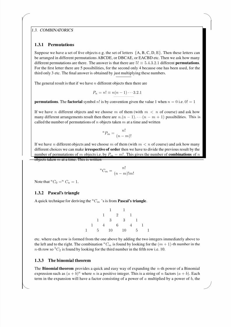
1.3.2 Pascal’s triangle
A quick technique for deriving the nC m ’s is from Pascal’s triangle.
1 11 2 1
1 3 3 11 4 6 4 1
1 5 10 10 5 1
etc. where each row is formed from the one above by adding the two integers immediately above to
the left and to the right. The combination nC m is found by looking for the (m + 1)-th number in the
n-th row so 5C 2 is found by looking for the third number in the fifth row i.e. 10.
1.3.3 The binomial theorem
The Binomial theorem provides a quick and easy way of expanding the n-th power of a Binomial
expression such as (a + b)n where n is a positive integer. This is a string of n factors (a + b). Each
term in the expansion will have a factor consisting of a power of a multiplied by a power of b, the
8/6/2019 A 107 Math 2008 Lecture Notes
http://slidepdf.com/reader/full/a-107-math-2008-lecture-notes 14/84
'
&
$
%
14 CHAPTER 1. BASIC MATHS COURSE
powers adding up to to n e.g. one such term is an−s bs with 0 ≤ s ≤ n. The number of different
ways of getting a contribution to this term is calculated by counting the number of different ways of
choosing exactlys
factors of b
from then
factors which make up the original expression i.e. n
C s. The
final result is the binomial theorem which states:
(a + b)n =n
s=0
nC s an−s bs
An example follows: (a + b)5 = a5 + 5 a4 b + 10 a3 b2 + 10 a2 b3 + 5 a b4 + b5.
(If n is not a positive integer a form of the Binomial Theorem still holds but we do not discuss it
here.)
1.4 Functions and graphs
A function is a recipe or method for finding the value of one variable y if you are given the value of
another variable x. The variable x is called the independent variable and y is called the dependent
variable. The independent variable x is sometimes called the argument of the function. The rela-
tionship between the two variables is often written y = f (x).
The recipe does not have to be expressed in algebraic terms but it must give a single definite answer.
Here are some examples:
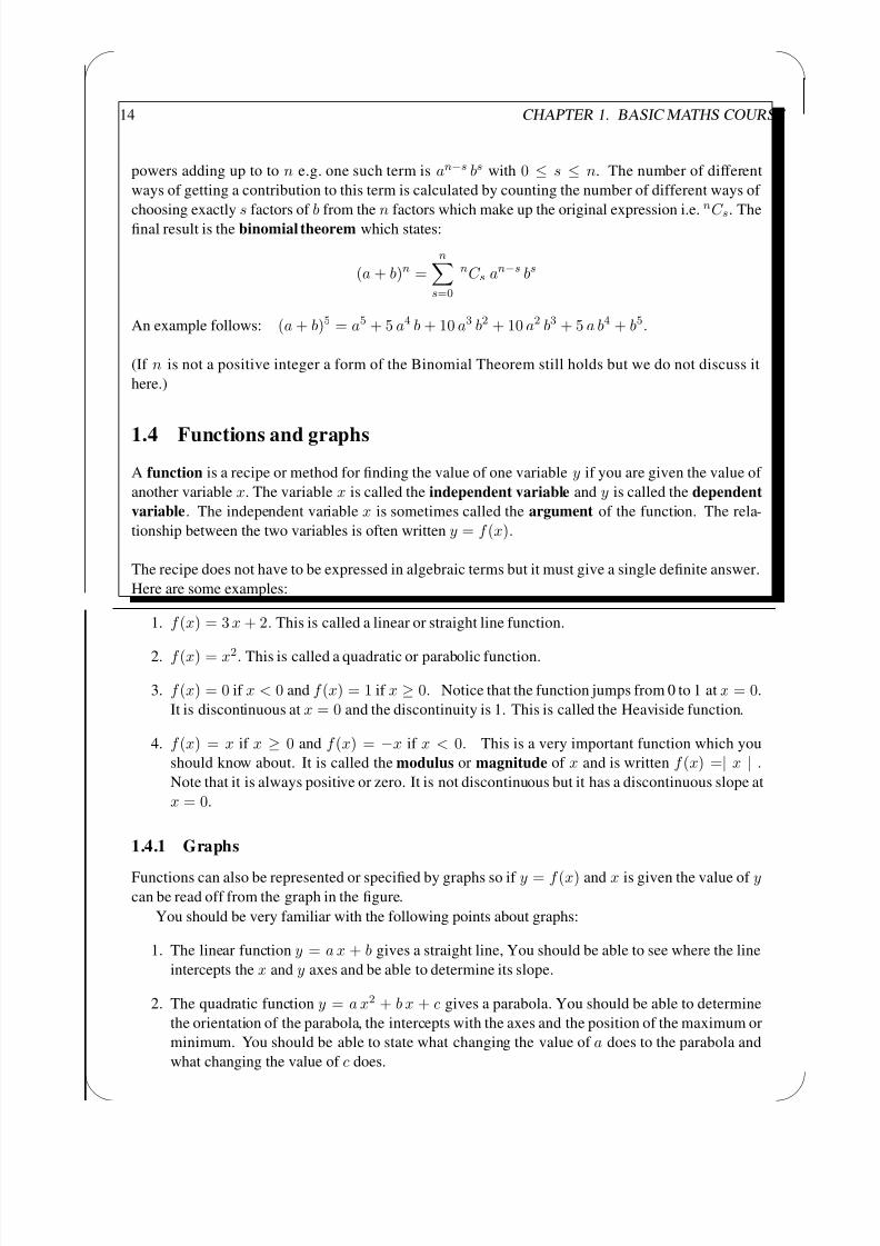
1. f (x) = 3 x + 2. This is called a linear or straight line function.
2. f (x) = x2. This is called a quadratic or parabolic function.
3. f (x) = 0 if x < 0 and f (x) = 1 if x ≥ 0. Notice that the function jumps from 0 to 1 at x = 0.
It is discontinuous at x = 0 and the discontinuity is 1. This is called the Heaviside function.
4. f (x) = x if x ≥ 0 and f (x) = −x if x < 0. This is a very important function which you
should know about. It is called the modulus or magnitude of x and is written f (x) =| x | .Note that it is always positive or zero. It is not discontinuous but it has a discontinuous slope at
x = 0.
1.4.1 Graphs
Functions can also be represented or specified by graphs so if y = f (x) and x is given the value of ycan be read off from the graph in the figure.
You should be very familiar with the following points about graphs:
1. The linear function y = a x + b gives a straight line, You should be able to see where the line
intercepts the x and y axes and be able to determine its slope.
2. The quadratic function y = a x2 + b x + c gives a parabola. You should be able to determine
the orientation of the parabola, the intercepts with the axes and the position of the maximum or
minimum. You should be able to state what changing the value of a does to the parabola and
what changing the value of c does.
8/6/2019 A 107 Math 2008 Lecture Notes
http://slidepdf.com/reader/full/a-107-math-2008-lecture-notes 15/84
'
&
$
%
1.4. FUNCTIONS AND GRAPHS 15
3. You should be able to draw rough graphs of y = xn and y = x−n for any positive integral value
of n.
4. If you have the graph of a function y = f (x) and two numbers a and b (which can be positive,
negative or zero) you should immediately be able to say what the effect of each of the following
transformations is: y = f (x + a), y = f (x) + a, y = f (b x). y = b f (x), x = f (y).
5. If you have a relation y = a xb and you take logarithms you get ln y = b ln x + ln a. Now
write Y = ln y, X = ln x and A = ln a so that the equation becomes Y = b X + A and draw
a graph of Y against X which is a straight line. From the intercept with the Y axis you can
determine A and hence a and from the slope you can determine b. This method is very useful in
analysing experimental results. It is called a log-log plot. If you have a straight line in a log-log
plot it tells you that you have a power law between y and x.
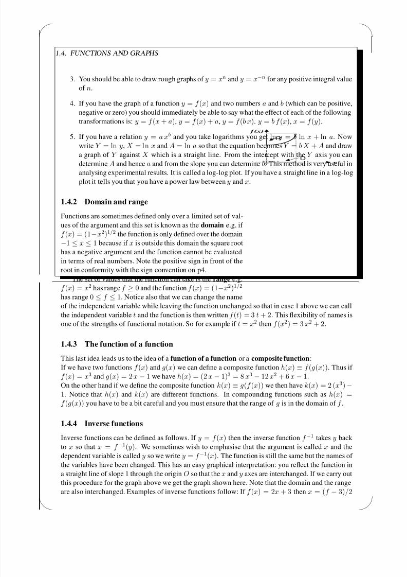
1.4.2 Domain and range
Functions are sometimes defined only over a limited set of val-
ues of the argument and this set is known as the domain e.g. if
f (x) = (1−x2)1/2 the function is only defined over the domain
−1 ≤ x ≤ 1 because if x is outside this domain the square root
has a negative argument and the function cannot be evaluated
in terms of real numbers. Note the positive sign in front of the
root in conformity with the sign convention on p4.
The set of values that the function can take is the range e.g.
f (x) = x2 has range f ≥ 0 and the function f (x) = (1−x2)1/2
has range 0
≤f
≤1. Notice also that we can change the name
of the independent variable while leaving the function unchanged so that in case 1 above we can call
the independent variable t and the function is then written f (t) = 3 t + 2. This flexibility of names is
one of the strengths of functional notation. So for example if t = x2 then f (x2) = 3 x2 + 2.
1.4.3 The function of a function
This last idea leads us to the idea of a function of a function or a composite function:
If we have two functions f (x) and g(x) we can define a composite function h(x) ≡ f (g(x)). Thus if
f (x) = x3 and g(x) = 2 x − 1 we have h(x) = (2 x − 1)3 = 8 x3 − 12 x2 + 6 x − 1.On the other hand if we define the composite function k(x) ≡ g(f (x)) we then have k(x) = 2 (x3) −1. Notice that h(x) and k(x) are different functions. In compounding functions such as h(x) =
f (g(x)) you have to be a bit careful and you must ensure that the range of g is in the domain of f .
1.4.4 Inverse functions
Inverse functions can be defined as follows. If y = f (x) then the inverse function f −1 takes y back
to x so that x = f −1(y). We sometimes wish to emphasise that the argument is called x and the
dependent variable is called y so we write y = f −1(x). The function is still the same but the names of
the variables have been changed. This has an easy graphical interpretation: you reflect the function in
a straight line of slope 1 through the origin O so that the x and y axes are interchanged. If we carry out
this procedure for the graph above we get the graph shown here. Note that the domain and the range
are also interchanged. Examples of inverse functions follow: If f (x) = 2x + 3 then x = (f − 3)/2
8/6/2019 A 107 Math 2008 Lecture Notes
http://slidepdf.com/reader/full/a-107-math-2008-lecture-notes 16/84
'
&
$
%
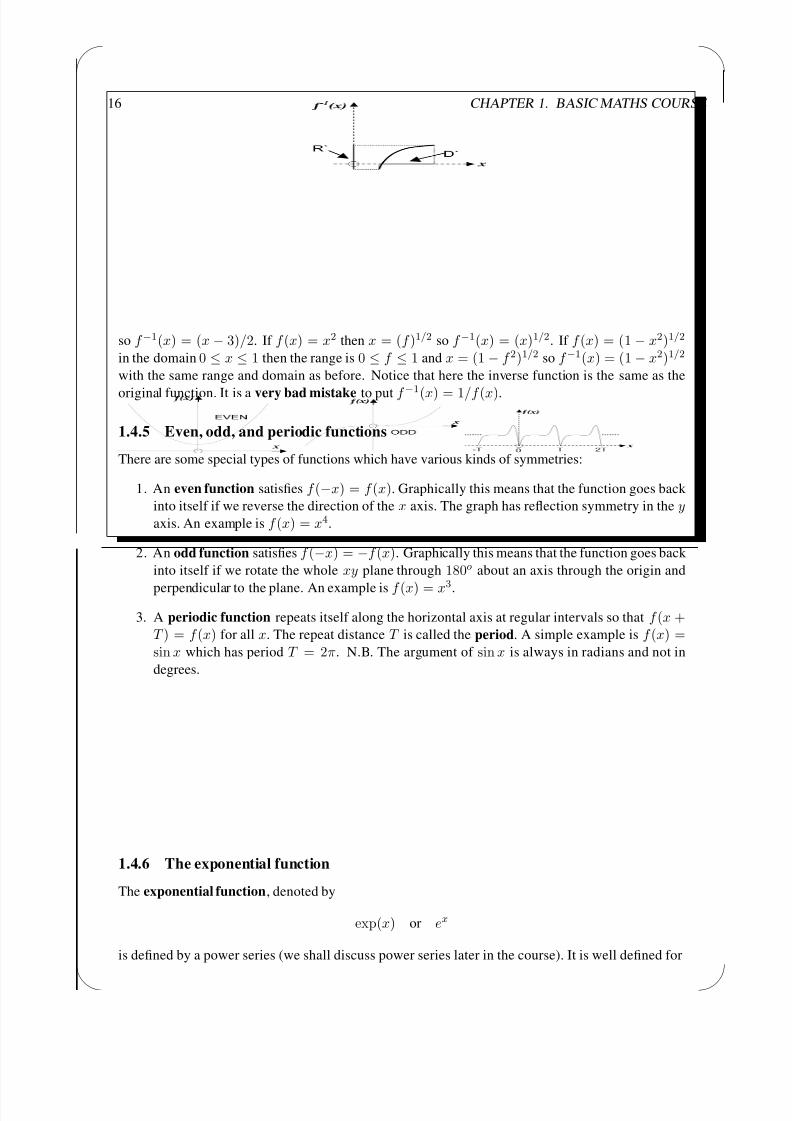
16 CHAPTER 1. BASIC MATHS COURSE
so f −1(x) = (x − 3)/2. If f (x) = x2 then x = (f )1/2 so f −1(x) = (x)1/2. If f (x) = (1 − x2)1/2
in the domain 0 ≤ x ≤ 1 then the range is 0 ≤ f ≤ 1 and x = (1 − f 2)1/2 so f −1(x) = (1 − x2)1/2
with the same range and domain as before. Notice that here the inverse function is the same as the
original function. It is a very bad mistake to put f −1(x) = 1/f (x).
1.4.5 Even, odd, and periodic functions
There are some special types of functions which have various kinds of symmetries:
1. An even function satisfies f (−x) = f (x). Graphically this means that the function goes back
into itself if we reverse the direction of the x axis. The graph has reflection symmetry in the yaxis. An example is f (x) = x4.
2. An odd function satisfies f (−x) = −f (x). Graphically this means that the function goes back
into itself if we rotate the whole xy plane through 180o about an axis through the origin and
perpendicular to the plane. An example is f (x) = x3.
3. A periodic function repeats itself along the horizontal axis at regular intervals so that f (x +T ) = f (x) for all x. The repeat distance T is called the period. A simple example is f (x) =sin x which has period T = 2π. N.B. The argument of sin x is always in radians and not in
degrees.
1.4.6 The exponential function
The exponential function, denoted by
exp(x) or ex
is defined by a power series (we shall discuss power series later in the course). It is well defined for
8/6/2019 A 107 Math 2008 Lecture Notes
http://slidepdf.com/reader/full/a-107-math-2008-lecture-notes 17/84
'
&
$
%
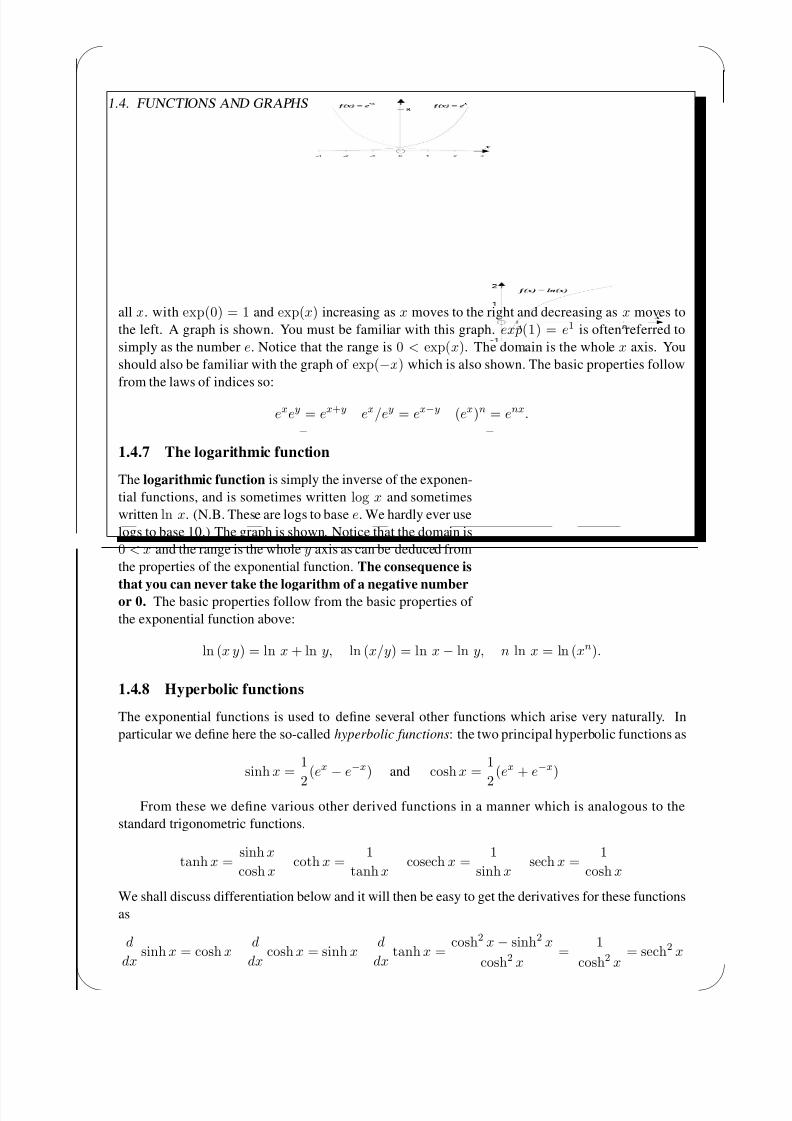
1.4. FUNCTIONS AND GRAPHS 17
all x. with exp(0) = 1 and exp(x) increasing as x moves to the right and decreasing as x moves to
the left. A graph is shown. You must be familiar with this graph. exp(1) = e1 is often referred to
simply as the number e. Notice that the range is 0 < exp(x). The domain is the whole x axis. You
should also be familiar with the graph of exp(−x) which is also shown. The basic properties follow
from the laws of indices so:
exey = ex+y ex/ey = ex−y (ex)n = enx.
1.4.7 The logarithmic function
The logarithmic function is simply the inverse of the exponen-
tial functions, and is sometimes written log x and sometimes
written ln x. (N.B. These are logs to base e. We hardly ever use
logs to base 10.) The graph is shown. Notice that the domain is
0 < x and the range is the whole y axis as can be deduced from
the properties of the exponential function. The consequence is
that you can never take the logarithm of a negative numberor 0. The basic properties follow from the basic properties of
the exponential function above:
ln (x y) = ln x + ln y, ln (x/y) = ln x − ln y, n ln x = ln (xn).
1.4.8 Hyperbolic functions
The exponential functions is used to define several other functions which arise very naturally. In
particular we define here the so-called hyperbolic functions: the two principal hyperbolic functions as
sinh x =1
2
(ex
−e−x) and cosh x =
1
2
(ex + e−x)
From these we define various other derived functions in a manner which is analogous to the
standard trigonometric functions.
tanh x =sinh x
cosh xcoth x =
1
tanh xcosech x =
1
sinh xsech x =
1
cosh x
We shall discuss differentiation below and it will then be easy to get the derivatives for these functions
as
d
dxsinh x = cosh x
d
dxcosh x = sinh x
d
dxtanh x =
cosh2 x − sinh2 x
cosh2 x=
1
cosh2 x= sech2 x
8/6/2019 A 107 Math 2008 Lecture Notes
http://slidepdf.com/reader/full/a-107-math-2008-lecture-notes 18/84
'
&
$
%
18 CHAPTER 1. BASIC MATHS COURSE
Notice moreover that
cosh2 x − sinh2 x =1
4(ex + e−x)2 − 1
4(ex − e−x)2 = 1.
1.5 Cartesian (or Coordinate) Geometry
It is very natural for data to be expressed in the form of sets of numbers, such as a list of pairs (x, y)or triplets (x,y ,z) (or indeed an arbitrary number of terms (x , y , z , w . . .)). We are then interested in
representing such data in some form, in other words we think of each pair (x, y) or triplet (x,y,z) as
part of a space of all possible pairs or triplets (or quadruplets. . . ). We concentrate here on the case
of pairs (x, y) but the other cases are very similar although much more difficult to visualize. First we
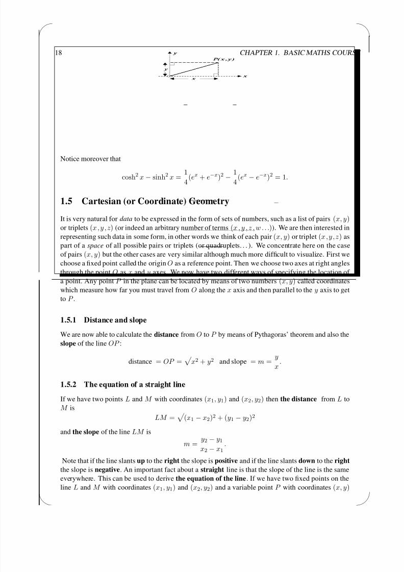
choose a fixed point called the origin O as a reference point. Then we choose two axes at right angles
through the point O as x and y axes. We now have two different ways of specifying the location of
a point. Any point P in the plane can be located by means of two numbers (x, y) called coordinates
which measure how far you must travel from O along the x axis and then parallel to the y axis to get
to P .
1.5.1 Distance and slope
We are now able to calculate the distance from O to P by means of Pythagoras’ theorem and also the
slope of the line OP :
distance = OP =
x2 + y2 and slope = m =y
x.
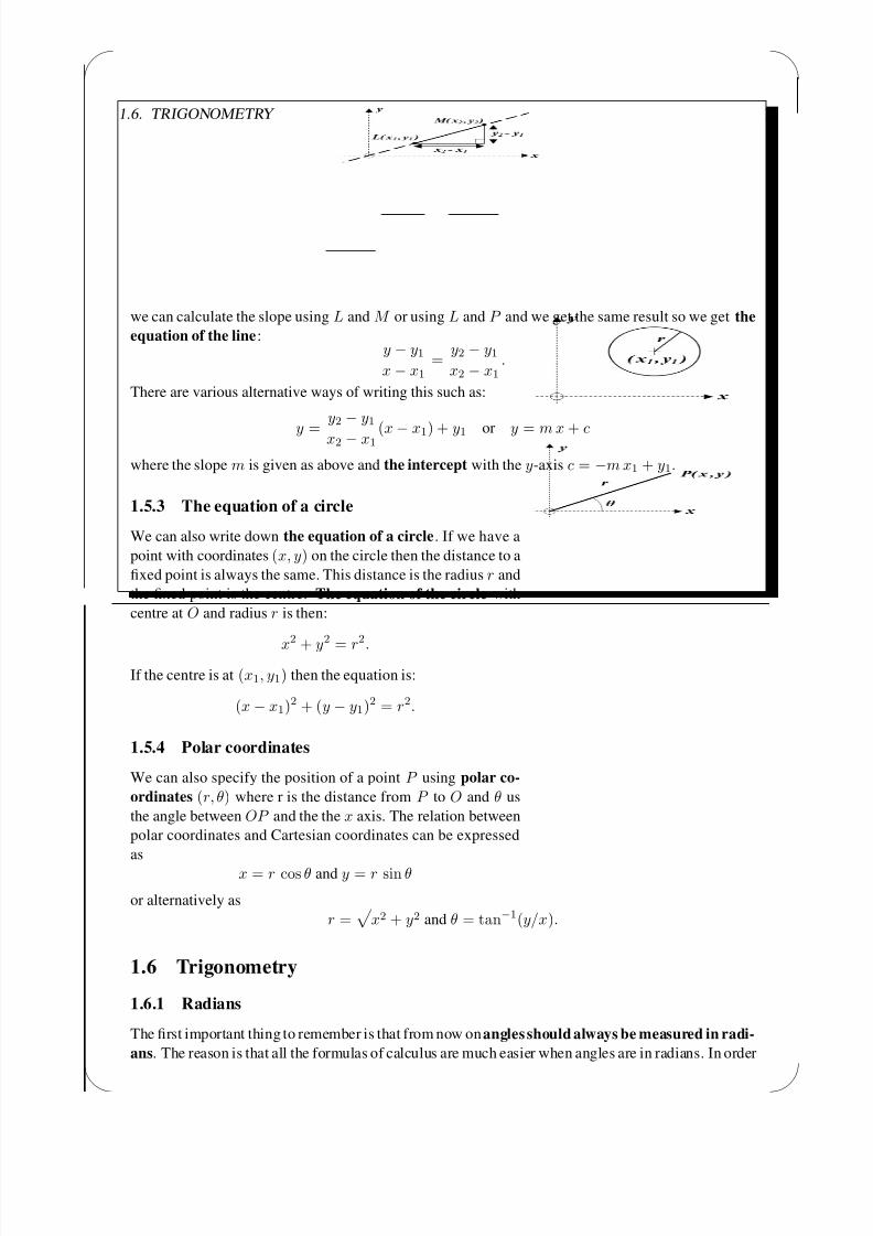
1.5.2 The equation of a straight line
If we have two points L and M with coordinates (x1, y1) and (x2, y2) then the distance from L toM is
LM =
(x1 − x2)2 + (y1 − y2)2
and the slope of the line LM is
m =y2 − y1x2 − x1
.
Note that if the line slants up to the right the slope is positive and if the line slants down to the right
the slope is negative. An important fact about a straight line is that the slope of the line is the same
everywhere. This can be used to derive the equation of the line. If we have two fixed points on the
line L and M with coordinates (x1, y1) and (x2, y2) and a variable point P with coordinates (x, y)
8/6/2019 A 107 Math 2008 Lecture Notes
http://slidepdf.com/reader/full/a-107-math-2008-lecture-notes 19/84
'
&
$
%
1.6. TRIGONOMETRY 19
we can calculate the slope using L and M or using L and P and we get the same result so we get the
equation of the line:y − y1x − x1
=y2 − y1x2 − x1
.
There are various alternative ways of writing this such as:
y =
y2
−y1
x2 − x1 (x − x1) + y1 or y = m x + c
where the slope m is given as above and the intercept with the y-axis c = −m x1 + y1.
1.5.3 The equation of a circle
We can also write down the equation of a circle. If we have a
point with coordinates (x, y) on the circle then the distance to a
fixed point is always the same. This distance is the radius r and
the fixed point is the centre. The equation of the circle with
centre at O and radius r is then:
x2
+ y2
= r2
.If the centre is at (x1, y1) then the equation is:
(x − x1)2 + (y − y1)2 = r2.
1.5.4 Polar coordinates
We can also specify the position of a point P using polar co-
ordinates (r, θ) where r is the distance from P to O and θ us
the angle between OP and the the x axis. The relation between
polar coordinates and Cartesian coordinates can be expressed
as
x = r cos θ and y = r sin θ
or alternatively as
r =
x2 + y2 and θ = tan−1(y/x).
1.6 Trigonometry
1.6.1 Radians
The first important thing to remember is that from now on angles should always be measured in radi-
ans. The reason is that all the formulas of calculus are much easier when angles are in radians. In order
8/6/2019 A 107 Math 2008 Lecture Notes
http://slidepdf.com/reader/full/a-107-math-2008-lecture-notes 20/84
'
&
$
%
20 CHAPTER 1. BASIC MATHS COURSE
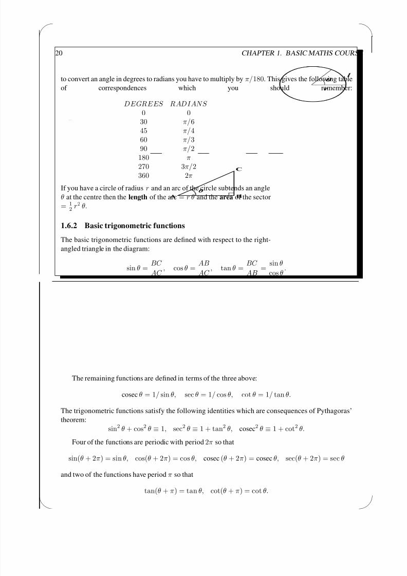
to convert an angle in degrees to radians you have to multiply by π/180. This gives the following table
of correspondences which you should remember:
DEGREES RADIANS 0 0
30 π/645 π/460 π/390 π/2
180 π270 3π/2360 2π
If you have a circle of radius r and an arc of the circle subtends an angle
θ at the centre then the length of the arc = r θ and the area of the sector
= 12 r2 θ.
1.6.2 Basic trigonometric functions
The basic trigonometric functions are defined with respect to the right-
angled triangle in the diagram:
sin θ =BC
AC , cos θ =
AB
AC , tan θ =
BC
AB=
sin θ
cos θ.
The remaining functions are defined in terms of the three above:
cosec θ = 1/ sin θ, sec θ = 1/ cos θ, cot θ = 1/ tan θ.
The trigonometric functions satisfy the following identities which are consequences of Pythagoras’
theorem:
sin2 θ + cos2 θ ≡ 1, sec2 θ ≡ 1 + tan2 θ, cosec2 θ ≡ 1 + cot2 θ.
Four of the functions are periodic with period 2π so that
sin(θ + 2π) = sin θ, cos(θ + 2π) = cos θ, cosec (θ + 2π) = cosec θ, sec(θ + 2π) = sec θ
and two of the functions have period π so that
tan(θ + π) = tan θ, cot(θ + π) = cot θ.
8/6/2019 A 107 Math 2008 Lecture Notes
http://slidepdf.com/reader/full/a-107-math-2008-lecture-notes 21/84
'
&
$
%
1.6. TRIGONOMETRY 21
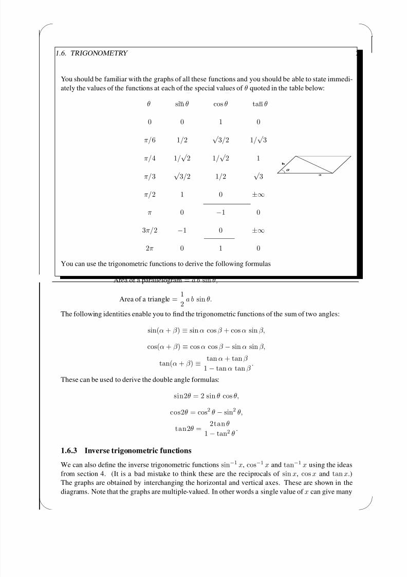
You should be familiar with the graphs of all these functions and you should be able to state immedi-
ately the values of the functions at each of the special values of θ quoted in the table below:
θ sin θ cos θ tan θ
0 0 1 0
π/6 1/2√
3/2 1/√
3
π/4 1/√
2 1/√
2 1
π/3√
3/2 1/2√
3
π/2 1 0
±∞π 0 −1 0
3π/2 −1 0 ±∞
2π 0 1 0
You can use the trigonometric functions to derive the following formulas
Area of a parallelogram = a b sin θ,
Area of a triangle =1
2a b sin θ.
The following identities enable you to find the trigonometric functions of the sum of two angles:
sin(α + β ) ≡ sin α cos β + cos α sin β,
cos(α + β ) ≡ cos α cos β − sin α sin β,
tan(α + β ) ≡ tan α + tan β
1 − tan α tan β .
These can be used to derive the double angle formulas:
sin2θ = 2 sin θ cos θ,
cos2θ = cos2 θ − sin2 θ,
tan2θ =2tan θ
1 − tan2 θ.
1.6.3 Inverse trigonometric functions
We can also define the inverse trigonometric functions sin−1 x, cos−1 x and tan−1 x using the ideas
from section 4. (It is a bad mistake to think these are the reciprocals of sin x, cos x and tan x.)
The graphs are obtained by interchanging the horizontal and vertical axes. These are shown in the
diagrams. Note that the graphs are multiple-valued. In other words a single value of x can give many
8/6/2019 A 107 Math 2008 Lecture Notes
http://slidepdf.com/reader/full/a-107-math-2008-lecture-notes 22/84
'
&
$
%
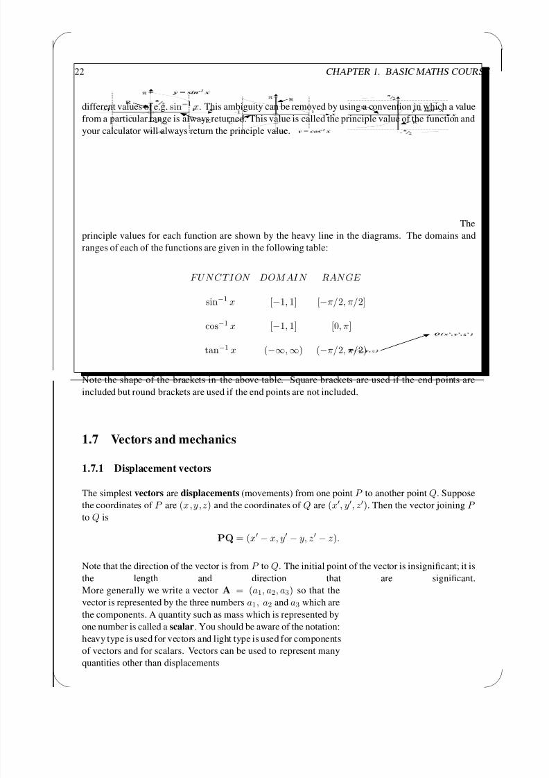
22 CHAPTER 1. BASIC MATHS COURSE
different values of e.g. sin−1 x. This ambiguity can be removed by using a convention in which a value
from a particular range is always returned. This value is called the principle value of the function and
your calculator will always return the principle value.
The
principle values for each function are shown by the heavy line in the diagrams. The domains and
ranges of each of the functions are given in the following table:
F U N C T I ON DOM AI N RAN GE
sin−1 x [−1, 1] [−π/2, π/2]
cos−1 x [−1, 1] [0, π]
tan−1 x (−∞, ∞) (−π/2, π/2)
Note the shape of the brackets in the above table. Square brackets are used if the end points are
included but round brackets are used if the end points are not included.
1.7 Vectors and mechanics
1.7.1 Displacement vectors
The simplest vectors are displacements (movements) from one point P to another point Q. Suppose
the coordinates of P are (x,y,z) and the coordinates of Q are (x, y, z). Then the vector joining P to Q is
PQ = (x
−x, y
−y, z
−z).
Note that the direction of the vector is from P to Q. The initial point of the vector is insignificant; it is
the length and direction that are significant.
More generally we write a vector A = (a1, a2, a3) so that the
vector is represented by the three numbers a1, a2 and a3 which are
the components. A quantity such as mass which is represented by
one number is called a scalar. You should be aware of the notation:
heavy type is used for vectors and light type is used for components
of vectors and for scalars. Vectors can be used to represent many
quantities other than displacements
8/6/2019 A 107 Math 2008 Lecture Notes
http://slidepdf.com/reader/full/a-107-math-2008-lecture-notes 23/84
'
&
$
%
1.7. VECTORS AND MECHANICS 23
1.7.2 The magnitude of a vector
The length of the vector is written
|A
|≡ a21 + a22 + a23. This is sometimes called the magnitude
or modulus of the vector. The quantity
A ≡ A
| A | =
a1
| A | ,a2
| A | ,a3
| A |
is called the unit vector in the direction of A. The components of A such as a1/ | A | etc. are called
the direction cosines of A and give its direction.
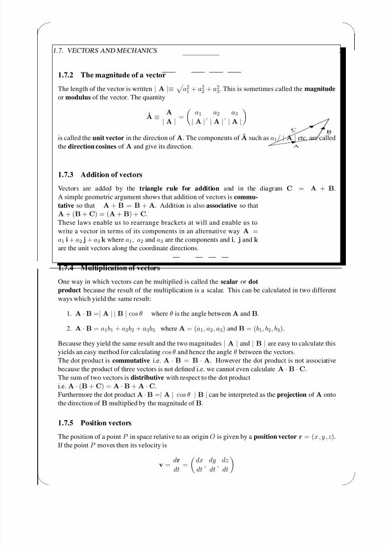
1.7.3 Addition of vectors
Vectors are added by the triangle rule for addition and in the diagram C = A + B.
A simple geometric argument shows that addition of vectors is commu-
tative so that A + B = B + A. Addition is also associative so that
A + (B + C) = (A + B) + C.
These laws enable us to rearrange brackets at will and enable us to
write a vector in terms of its components in an alternative way A =a1 i+ a2 j+ a3 k where a1, a2 and a3 are the components and i, j and k
are the unit vectors along the coordinate directions.
1.7.4 Multiplication of vectors
One way in which vectors can be multiplied is called the scalar or dot
product because the result of the multiplication is a scalar. This can be calculated in two differentways which yield the same result:
1. A ·B =| A | | B | cos θ where θ is the angle between A and B.
2. A ·B = a1b1 + a2b2 + a3b3 where A = (a1, a2, a3) and B = (b1, b2, b3).
Because they yield the same result and the two magnitudes | A | and | B | are easy to calculate this
yields an easy method for calculating cos θ and hence the angle θ between the vectors.
The dot product is commutative i.e. A · B = B · A. However the dot product is not associative
because the product of three vectors is not defined i.e. we cannot even calculate A ·B ·C.
The sum of two vectors is distributive with respect to the dot product
i.e. A · (B+ C) = A ·B+ A ·C.Furthermore the dot product A ·B =| A | cos θ | B | can be interpreted as the projection of A onto
the direction of B multiplied by the magnitude of B.
1.7.5 Position vectors
The position of a point P in space relative to an origin O is given by a position vector r = (x,y ,z).
If the point P moves then its velocity is
v =dr
dt=
dx
dt,
dy
dt,
dz
dt
8/6/2019 A 107 Math 2008 Lecture Notes
http://slidepdf.com/reader/full/a-107-math-2008-lecture-notes 24/84
'
&
$
%
24 CHAPTER 1. BASIC MATHS COURSE
and its acceleration is
a =d2r
dt2=
d2x
dt2,
d2y
dt2,
d2z
dt2 .
This tells you that vectors can be used to represent directed quantities other than displacements such
as velocities, accelerations, forces, electric fields etc.
1.7.6 Circular motion
We can use some of these ideas to discuss circular motion such as the motion of a stone on a string
or a planet around the sun. Suppose a point P moves in a circle of radius r around the origin O with
constant speed v then the following relationships hold:
v = r ω and a = v2/r and a = r ω2
where a is the acceleration of P toward the centre and ω is the angular velocity of the point P aboutO i.e. the rate of change with respect to time of the angle subtended by the path of P at O. Notice
that the magnitude of the acceleration is constant but the direction is constantly changing as P moves
around the centre. If the circular path is in the xy plane we can also write down the components of
the position vector of P :x(t) = r cos ω t and y(t) = r sin ω t
where we have assumed that the particle starts off on the x axis and moves in the counter-clockwise
direction. It is easy to make the necessary modifications if these last two assumptions are relaxed.
1.7.7 Constant acceleration
If on the other hand the point moves under an acceleration which is constant in magnitude and di-
rection then the velocity and position vector of the point as a function of time t (i.e. the path of the
particle) are given by the following two equations:
v = u + a t and r = r0 + u t + 12 a t2
where r0 and u are the position vector and velocity of the point at the initial time t = 0. It is easy to
show that the path is a parabola. If the acceleration and initial velocity are in the same direction we
can write these equations in the form:
v = u + a t and s = u t + 12 a t2
where s is the distance moved from the initial point.
1.7.8 Newton’s laws
In order to discuss Mechanics you need Newton’s three laws of motion:
1. A body continues in its state of rest or uniform motion unless acted upon by an external force.
2. If a body is acted on by a force the acceleration is proportional to the force and in the same
direction.
This can be expressed in vector form as F = ma where the constant of proportionality is the
mass of the body.
8/6/2019 A 107 Math 2008 Lecture Notes
http://slidepdf.com/reader/full/a-107-math-2008-lecture-notes 25/84
'
&
$
%
1.8. LIMITS OF SEQUENCES 25
3. To every force there is an equal and opposite reaction.
You should be familiar with some commonly encountered forces:
1. The force of gravitation can often be approximated as uniform and in the downward direction
so F = −mg k.
2. The force of friction between two bodies in contact satisfies | F |≤ µR where R is the normal
reaction between the bodies and the direction of F is in the plane of contact of the bodies.
You should be familiar with the concept of equilibrium and you should be able to solve problems
of bodies in equilibrium using ideas such as the resolution of forces with respect to an axis and the
moment of forces about an axis.
You should be able to set up equations of motion for bodies out of equilibrium in the form of second
order differential equations using the fact that a = d2r/dt2. You should be able to solve these equa-
tions in simple cases.
You should be familiar with the ideas of energy E and momentum p = mv and able to apply
these ideas in situations where the energy or momentum are conserved.
1.8 Limits of sequences
A sequence is just an “ordered set” of numbers {x1, x2, x3, . . .} This sequence may be finite or infinite.
We sometimes write
{xk
}nk=1 =
{x1, x2, . . . , xn
}or
{xk
}∞k=1 =
{x1, x2, x3, . . .
}to denote a sequence of n numbers and an infinite sequence respectively. A simple example is the
sequence 1
k
∞k=1
=
1
1,
1
2,
1
3, . . .
.
The definition of a sequence does not require it to be defined according to any pattern or rule, any or-
dered set of numbers is a sequence. It is sometimes important to understand the asymptotic behaviour
of a sequence. We say that a sequence converges to a (unique) limit and write
xn → or limn→∞
xn =
if the values of the sequence get closer and closer to the value as n gets larger and larger . The
notion of a limit is absolutely crucial in all of modern mathematics and underlies all of differential
and integral calculus. In some cases the limit of a sequence is very easy to establish.
Example 2. 1. the sequence {1/k}∞k=1 tends to the limit = 0: limk→∞ 1/k = 0;
2. the sequence {1, 2, 3, . . .} = {k}∞k=1 tends to the limit = ∞: limk→∞ k = ∞;
3. the sequence {3+k2
k2 }∞k=1 tends to the limit = 5: limk→∞3+5k2
k2 = limk→∞3k2 + 5 = 5.
However the definitions is a little more subtle than appears at first sight and it is easy to construct
sequences whose asymptotic behaviour behaviour is not so straightforward so that the limit is harder
to establish or may not even exist at all.
8/6/2019 A 107 Math 2008 Lecture Notes
http://slidepdf.com/reader/full/a-107-math-2008-lecture-notes 26/84
'
&
$
%
26 CHAPTER 1. BASIC MATHS COURSE
Example 3. 1. {−1, +1, −1, +1, −1, . . .} = {(−1)k}∞k=1 does not tend to a limit.
2.
{(
−1)k + 1/k
}∞k=1 =
{0, 3/2,
−2/3, 5/4,
−4/5, 7/6, . . .
}does not tend to a limit since it has
a subsequence of negative numbers tending to 0 and a subsequence of positive numbers tending
to 2, so as a sequence itself it is not tending to any particular number.
It is beyond the scope of this course to analyse the notion of limit in more detail, and we will
therefore generally refer to it’s intuitive meaning.
8/6/2019 A 107 Math 2008 Lecture Notes
http://slidepdf.com/reader/full/a-107-math-2008-lecture-notes 27/84
'
&
$
%
Chapter 2
Derivatives
2.1 Definition and basic examples
2.1.1 The derivative as gradient
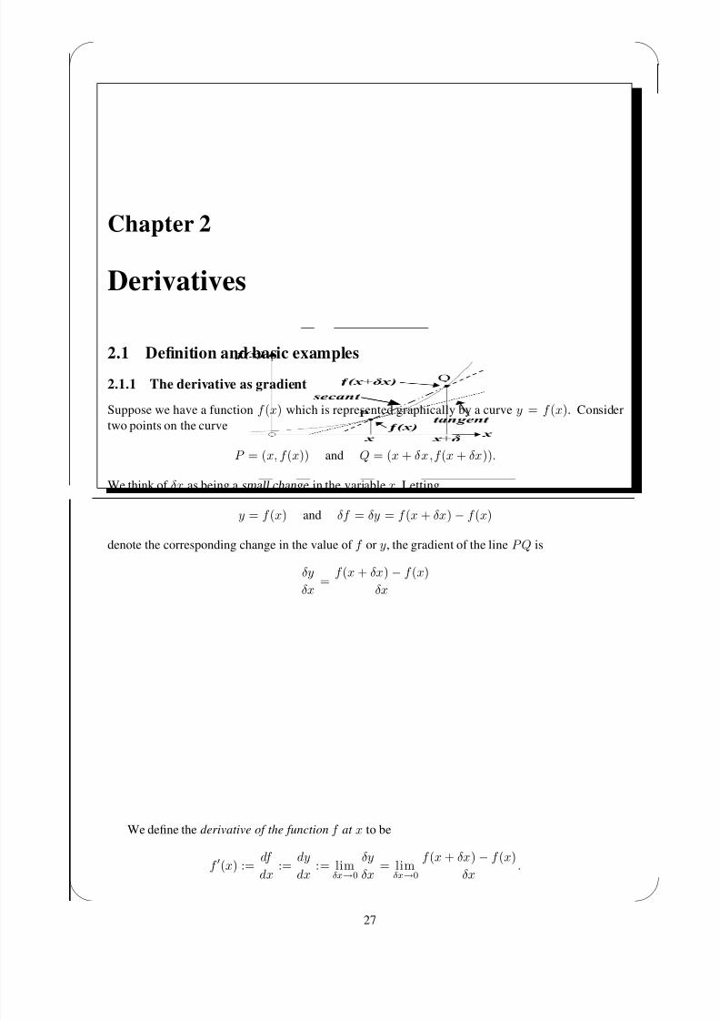
Suppose we have a function f (x) which is represented graphically by a curve y = f (x). Consider
two points on the curve
P = (x, f (x)) and Q = (x + δx,f (x + δx)).
We think of δx as being a small change in the variable x. Letting
y = f (x) and δf = δy = f (x + δx) − f (x)
denote the corresponding change in the value of f or y, the gradient of the line P Q is
δy
δx=
f (x + δx) − f (x)
δx
We define the derivative of the function f at x to be
f (x) :=df
dx:=
dy
dx:= lim
δx→0
δy
δx= lim
δx→0
f (x + δx) − f (x)
δx.
27
8/6/2019 A 107 Math 2008 Lecture Notes
http://slidepdf.com/reader/full/a-107-math-2008-lecture-notes 28/84
'
&
$
%
28 CHAPTER 2. DERIVATIVES
Geometrically this gives the limit of the gradients of the line P Q as δx gets smaller and smaller, or,
in other words, the gradient of the tangent to the graph of f at the point P . More formally, taking the
limitlimδx→0
as above means that we choose some discrete sequence of valuesδxn
withδxn → 0
,
consider the corresponding discrete sequence δf n and ask whether this sequence has a well defined
limit which is independent of the specific choice of sequence δxn. In particular the limit should not
depend on whether δx → 0 from above or from below.
It is important to appreciate that the derivative does not always exist.
Example 4. Consider the function f (x) = |x|. Let us try to evaluate the derivative at x = 0. Then
limx0
δf
δx= −1 = lim
x0
δf
δx= −1
Therefore this function is not differentiable at 0.
Differentiability of a function is a pointwise property. A function may be differentiable at some
points and not others as in the above examples. If we say that a function is differentiable we generally
mean that it is differentiable at every point of the domain. There exist functions which are continuous
but not differentiable at any point, for example the Weierstrass function.
2.1.2 Derivatives of special functions
We can actually compute the derivative of many functions directly from its definition, although we
often need some more results about the limits of functions which will be discussed in Chapter 5. We
discuss here one example that can be done directly.
Example 5. Let f (x) = xm with m ≥ 1 a positive integer. Then, by the binomial theorem in Section
1.3.3 we have
(x + δx)m = xm + mxm−1δx +m(m − 1)
2!xm−2(δx)2 + · · · + (δx)m.
Therefore
f (x + δx) − f (x)
δx=
(x + δx)m − xm
δx=
mxm−1δx + m(m−1)2! xm−2(δx)2 + · · · + (δx)m
δx= mxm−1 +
m(m − 1)
2!xm−2δx + · · · + (δx)m−1
As δx → 0 all terms containing δx also tend to 0 and therefore
f (x) = limδx→0
f (x + δx) − f (x)
δx= mxm−1.
You should also commit the following table of derivatives to memory. You will encounter
them very frequently in your course and you will be at a significant disadvantage later if you cannot
8/6/2019 A 107 Math 2008 Lecture Notes
http://slidepdf.com/reader/full/a-107-math-2008-lecture-notes 29/84
'
&
$
%
2.2. DIFFERENTIATING COMBINATIONS OF FUNCTIONS 29
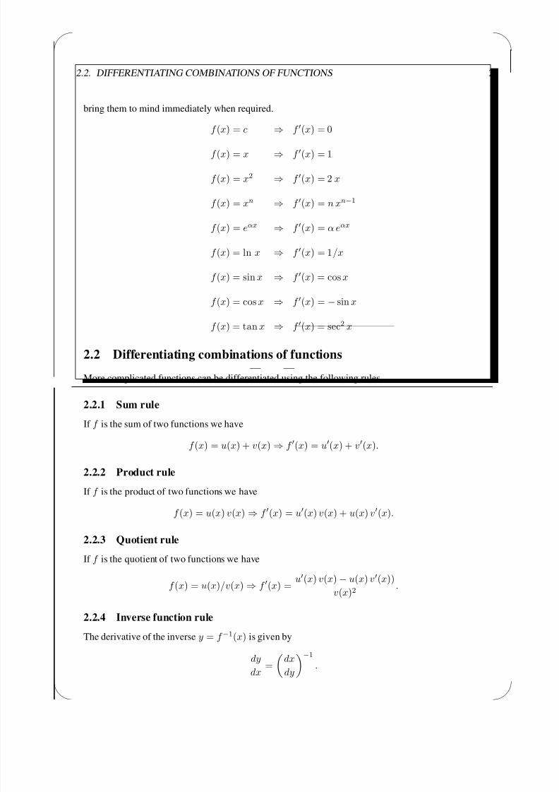
bring them to mind immediately when required.
f (x) = c
⇒f (x) = 0
f (x) = x ⇒ f (x) = 1
f (x) = x2 ⇒ f (x) = 2 x
f (x) = xn ⇒ f (x) = n xn−1
f (x) = eαx ⇒ f (x) = α eαx
f (x) = ln x ⇒ f (x) = 1/x
f (x) = sin x ⇒ f (x) = cos x
f (x) = cos x ⇒ f (x) = − sin x
f (x) = tan x ⇒ f (x) = sec2 x
2.2 Differentiating combinations of functions
More complicated functions can be differentiated using the following rules.
2.2.1 Sum rule
If f is the sum of two functions we have
f (x) = u(x) + v(x) ⇒ f (x) = u(x) + v(x).
2.2.2 Product rule
If f is the product of two functions we have
f (x) = u(x) v(x) ⇒ f (x) = u(x) v(x) + u(x) v(x).
2.2.3 Quotient rule
If f is the quotient of two functions we have
f (x) = u(x)/v(x) ⇒ f (x) =u(x) v(x) − u(x) v(x))
v(x)2.
2.2.4 Inverse function rule
The derivative of the inverse y = f −1(x) is given by
dy
dx=
dx
dy
−1.
8/6/2019 A 107 Math 2008 Lecture Notes
http://slidepdf.com/reader/full/a-107-math-2008-lecture-notes 30/84
'
&
$
%
30 CHAPTER 2. DERIVATIVES
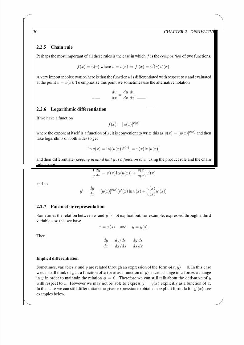
2.2.5 Chain rule
Perhaps the most important of all these rules is the case in which f is the composition of two functions.
f (x) = u(v) where v = v(x) ⇒ f (x) = u(v) v(x).
A very important observation here is that the function u is differentiated with respect to v and evaluated
at the point v = v(x). To emphasize this point we sometimes use the alternative notation
du
dx=
du
dv
dv
dx.
2.2.6 Logarithmic differentiation
If we have a function
f (x) = [u(x)]v(x)
where the exponent itself is a function of x, it is convenient to write this as y(x) = [u(x)]v(x) and then
take logarithms on both sides to get
ln y(x) = ln[(u(x))v(x)] = v(x)ln[u(x)]
and then differentiate (keeping in mind that y is a function of x) using the product rule and the chain
rule, to get
1
y
dy
dx= v(x)ln(u(x)) +
v(x)
u(x)u(x)
and so
y =dy
dx= [u(x)]v(x)[v(x) ln u(x) +
v(x)
u(x)u(x)].
2.2.7 Parametric representation
Sometimes the relation between x and y is not explicit but, for example, expressed through a third
variable s so that we have
x = x(s) and y = y(s).
Then
dydx
= dy/dsdx/ds
= dyds
dsdx
.
Implicit differentiation
Sometimes, variables x and y are related through an expression of the form φ(x, y) = 0. In this case
we can still think of y as a function of x (or x as a function of y) since a change in x forces a change
in y in order to maintain the relation φ = 0. Therefore we can still talk about the derivative of ywith respect to x. However we may not be able to express y = y(x) explicitly as a function of x.
In that case we can still differentiate the given expression to obtain an explicit formula for y(x), see
examples below.
8/6/2019 A 107 Math 2008 Lecture Notes
http://slidepdf.com/reader/full/a-107-math-2008-lecture-notes 31/84
'
&
$
%
2.2. DIFFERENTIATING COMBINATIONS OF FUNCTIONS 31
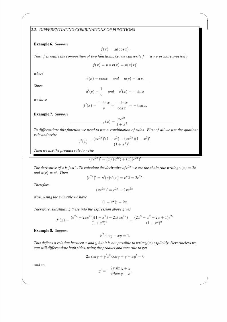
Example 6. Suppose
f (x) = ln(cos x).
Thus f is really the composition of two functions, i.e. we can write f = u ◦ v or more precisely
f (x) = u ◦ v(x) = u(v(x))
where
v(x) = cos x and u(v) = ln v.
Since
u(v) =1
vand v(x) = − sin x
we have
f (x) =− sin x
v=
− sin x
cos x= − tan x.
Example 7. Suppose
f (x) =xe2x
1 + x2
To differentiate this function we need to use a combination of rules. First of all we use the quotient
rule and write
f (x) =(xe2x)(1 + x2) − (xe2x)(1 + x2)
(1 + x2)2.
Then we use the product rule to write
(xe2x) = (x)(e2x) + (x)(e2x)
The derivative of x is just 1. To calculate the derivative of e2x
we use the chain rule writing v(x) = 2xand u(v) = ev. Then
(e2x) = u(v)v(x) = ev2 = 2e2x.
Therefore
(xe2x) = e2x + 2xe2x.
Now, using the sum rule we have
(1 + x2) = 2x.
Therefore, substituting these into the expression above gives
f (x) =(e2x + 2xe2x)(1 + x2) − 2x(xe2x)
(1 + x2)2=
(2x3 − x2 + 2x + 1)e2x
(1 + x2)2
Example 8. Suppose
x2 sin y + xy = 1.
This defines a relation between x and y but it is not possible to write y(x) explicitly. Nevertheless we
can still differentiate both sides, using the product and sum rule to get
2x sin y + yx2 cos y + y + xy = 0
and so
y = −2x sin y + y
x2cosy + x.
8/6/2019 A 107 Math 2008 Lecture Notes
http://slidepdf.com/reader/full/a-107-math-2008-lecture-notes 32/84
'
&
$
%
32 CHAPTER 2. DERIVATIVES
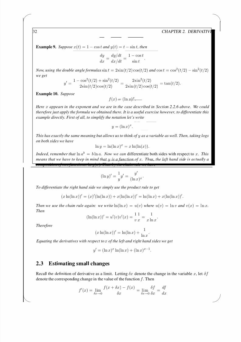
Example 9. Suppose x(t) = 1 − cos t and y(t) = t − sin t , then
dy
dx =
dy/dt
dx/dt =
1
−cos t
sin t .
Now, using the double angle formulas sin t = 2sin(t/2) cos(t/2) and cos t = cos2(t/2) − sin2(t/2)we get
y =1 − cos2(t/2) + sin2(t/2)
2sin(t/2)cos(t/2)=
2sin2(t/2)
2sin(t/2) cos(t/2)= tan(t/2).
Example 10. Suppose
f (x) = (ln x)x.
Here x appears in the exponent and we are in the case described in Section 2.2.6 above. We could
therefore just apply the formula we obtained there. It is a useful exercise however, to differentiate this
example directly. First of all, to simplify the notation let’s write
y = (ln x)x.
This has exactly the same meaning but allows us to think of y as a variable as well. Then, taking logs
on both sides we have
ln y = ln(ln x)x = x ln(ln(x)).
Indeed, remember that ln ab = b ln a. Now we can differentiate both sides with respect to x. This
means that we have to keep in mind that y is a function of x. Thus, the left hand side is actually a
composition of two functions: ln y(x). Thus by the chain rule we have
(ln y) =1
y
y =y
(ln x)x.
To differentiate the right hand side we simply use the product rule to get
(x ln(ln x)) = (x)(ln(ln x)) + x(ln(ln x)) = ln(ln x) + x(ln(ln x)).
Then we use the chain rule again: we write ln(ln x) = u(v) where u(v) = ln v and v(x) = ln x.
Then
(ln(ln x)) = u(v)v(x) =1
v
1
x=
1
x ln x.
Therefore
(x ln(ln x)) = ln(ln x) +1
ln x.
Equating the derivatives with respect to x of the left and right hand sides we get
y = (ln x)x ln(ln x) + (ln x)x−1.
2.3 Estimating small changes
Recall the definition of derivative as a limit. Letting δx denote the change in the variable x, let δf denote the corresponding change in the value of the function f . Then
f (x) = limδx→0
f (x + δx) − f (x)
δx= lim
δx→0
δf
δx=
df
dx
8/6/2019 A 107 Math 2008 Lecture Notes
http://slidepdf.com/reader/full/a-107-math-2008-lecture-notes 33/84
'
&
$
%
2.3. ESTIMATING SMALL CHANGES 33
Notice the difference betweenδf
δxand
df
dx.
The first expression is a real ratio between the two quantities δx and δf while the second is just a
notation to express the limit of these ratios as δx → 0; in particular df/dx may be an irrational
number and thus not expressible as a real ratio. Then, if δx is small we have
f (x) ≈ δf
δxand therefore f (x) · δx ≈ δf.
This can be used to estimate δf if df/dx is known.
Example 11. Let V (x) = x3 be the volume of cube with side length of x. Find approximate change
in volume as length of side goes from 2.0 to 2.01 cm. The derivative of V is V (x) = 3x2 and so
δV (x) ≈ V (x)δx
and
δV (2) ≈ V (2)δx = 1δx = 0.12
Example 12. The period T of small oscillations of a pendulum of length x is given by
T = 2π
x
g.
Show that if there is a small manufacturing error δx in the length x , producing an error of 1% (so
that δx/x = 1/100) , then the error in T is approximately 0.5%.
The definition of derivative
dT
dx= lim
δx→0
T (x + δx) − T (x)
δx,
means that
δT = T (x + δx) − T (x) ≈ dT
dxδx.
Differentiating T we get
dT
dx
=π
√xgand therefore
δT = T (x + δx) − T (x) ≈ dt
dxδx =
π√xg
δx.
Dividing through by T gives
δT
T ≈ π√
xg
1
2π
g
xδx =
1
2
δx
x= 1/200.
Hence the error in T is ≈ 0.5%.
8/6/2019 A 107 Math 2008 Lecture Notes
http://slidepdf.com/reader/full/a-107-math-2008-lecture-notes 34/84
'
&
$
%
34 CHAPTER 2. DERIVATIVES
2.4 Higher order derivatives
The derivative f of a function f is itself a function which may be differentiable, in which case we can
get the second order derivative f of f . If this second order derivative is differentiable we can get the
third order derivative and so on. In general we write
f (n) ordnf
dxn
to denote the nth order derivative of a function f (assuming that f, f , f , . . . , f (n−1) are all differ-
entiable). The higher order derivatives of simple or composite functions can of course be calculated
in principle by repeated differentiation but sometimes we can find particularly simple and elegant
formulae.
2.4.1 Induction
Sometimes we can find formulae for higher order derivative by induction.
Example 13. We show that for any n ≥ 1 we have
dn
dxnsin x = sin
x + n
π
2
.
We can show this by induction. For n = 1 we have
sin
x +π
2
= sin x cos
π
2+ cos x sin
π
2= cos x =
d
dxsin x.
Now, supposing this is true for some n−
1≥
1 we have
dn sin x
dxn=
d
dx
dn−1 sin x
dxn−1
=
d
dxsin
x + (n − 1)π
2
= cos
x + (n − 1)
π
2
But
cos
x + (n − 1)π
2
= sin
x + (n − 1)
π
2+
π
2
= sin
x + n
π
2
.
2.4.2 Leibniz’ rule
For the product of two functions we can find a particularly simple and elegant formula. Recall that
the product rule says
(f g) = f g + f g.
Then, by the product and sum rule we get
(f g) = (f g) + (f g) = f g + f g + gf + df = f g + 2f g + gf.
Iterating this procedure once again we get
(f g) = (f g) + (2f g) + (gf ) = f g + 3f g + 3f g + f g
Compare this to the following expression which follow from the Binomial Theorem in Section 1.3.3:
(a + b)2 = a2b0 + 2a1b1 + a0b2 and (a + b)3 = a3b0 + 3a2b1 + 3a1b2 + a0b3. From this we get the
general formula known as Leibniz Rule: For any n > 1
8/6/2019 A 107 Math 2008 Lecture Notes
http://slidepdf.com/reader/full/a-107-math-2008-lecture-notes 35/84
'
&
$
%
2.4. HIGHER ORDER DERIVATIVES 35
(f g)(n) = f (n)g +n1 f (n−1)g + ... +
nr f (n−r)g(r) + ... + f g(n)
where
nr
= n!
(n−r)!r! Sometimes we write D = ddx and so this becomes
Dn(f g) = (f g)(n) = Dn(f g)g +
n1
Dn−1f Dg + ... + f Dng
Example 14. Find Dn(exx2). Then Dn(ex) = ex , D(x2) = 2x , D2(x2) = 2 and so
Dn(exx2) = exx2 +
n1
ex2x +
n2
ex2 +
n3
ex0 + ... + 0
= ex
x2
+ 2xn
1
+ 2n
2
)

8/6/2019 A 107 Math 2008 Lecture Notes
http://slidepdf.com/reader/full/a-107-math-2008-lecture-notes 36/84
'
&
$
%
36CHAPTER 2. DERIVATIVES
8/6/2019 A 107 Math 2008 Lecture Notes
http://slidepdf.com/reader/full/a-107-math-2008-lecture-notes 37/84
'
&
$
%
Chapter 3
Integrals
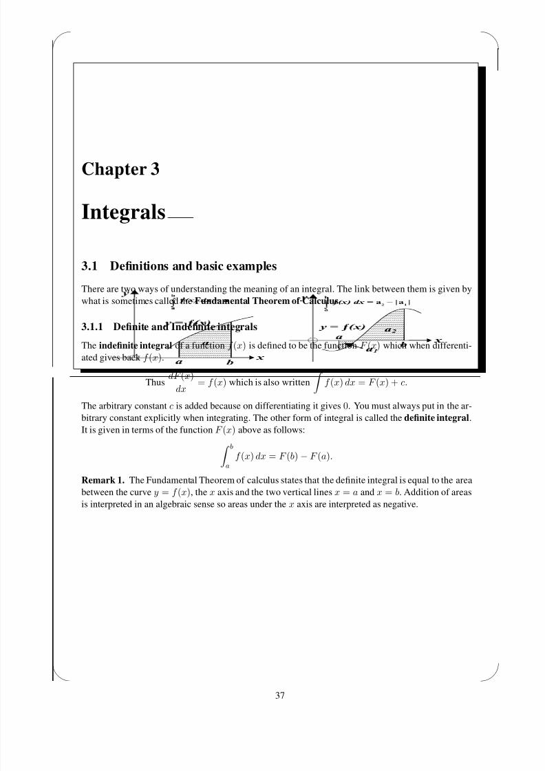
3.1 Definitions and basic examplesThere are two ways of understanding the meaning of an integral. The link between them is given by
what is sometimes called the Fundamental Theorem of Calculus.
3.1.1 Definite and Indefinite integrals
The indefinite integral of a function f (x) is defined to be the function F (x) which when differenti-
ated gives back f (x).
ThusdF (x)
dx= f (x) which is also written
f (x) dx = F (x) + c.
The arbitrary constant c is added because on differentiating it gives 0. You must always put in the ar-bitrary constant explicitly when integrating. The other form of integral is called the definite integral.
It is given in terms of the function F (x) above as follows: ba
f (x) dx = F (b) − F (a).
Remark 1. The Fundamental Theorem of calculus states that the definite integral is equal to the area
between the curve y = f (x), the x axis and the two vertical lines x = a and x = b. Addition of areas
is interpreted in an algebraic sense so areas under the x axis are interpreted as negative.
37
8/6/2019 A 107 Math 2008 Lecture Notes
http://slidepdf.com/reader/full/a-107-math-2008-lecture-notes 38/84
'
&
$
%
38 CHAPTER 3. INTEGRALS
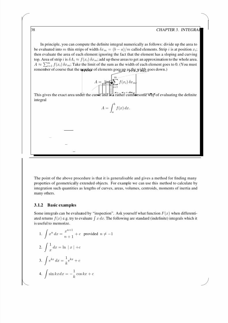
In principle, you can compute the definite integral numerically as follows: divide up the area to
be evaluated into m thin strips of width δxm = (b − a)/m called elements. Strip i is at position xi;
then evaluate the area of each element ignoring the fact that the element has a sloping and curving
top. Area of strip i is δAi ≈ f (xi) δxm; add up these areas to get an approximation to the whole area.
A ≈ mi=1 f (xi) δxm; Take the limit of the sum as the width of each element goes to 0. (You must
remember of course that the number of elements goes up as the width goes down.)
A = limm→∞
mi=1
f (xi) δxm.
This gives the exact area under the curve and is a rather cumbersome way of evaluating the definite
integral
A = b
a
f (x) dx.
The point of the above procedure is that it is generalisable and gives a method for finding many
properties of geometrically extended objects. For example we can use this method to calculate by
integration such quantities as lengths of curves, areas, volumes, centroids, moments of inertia and
many others.
3.1.2 Basic examples
Some integrals can be evaluated by “inspection”. Ask yourself what function F (x) when differenti-
ated returns f (x) e.g. try to evaluate
x dx. The following are standard (indefinite) integrals which it
is useful to memorize.
1.
xn dx =
xn+1
n + 1+ c provided n = −1
2.
1
xdx = ln | x | +c
3.
ekx dx =
1
kekx + c
4.
sin kxdx = −1
kcos kx + c
8/6/2019 A 107 Math 2008 Lecture Notes
http://slidepdf.com/reader/full/a-107-math-2008-lecture-notes 39/84
'
&
$
%
3.2. BASIC TECHNIQUES 39
5.
cos kxdx =
1
ksin kx + c
6.
sec x dx = ln | sec x + tan x | +c
7.
1
a2 + x2dx =
1
atan−1
x
a+ c
3.2 Basic techniques
There are several “tricks” to integrate more complicated composite functions. Unfortunately there is
no general systematic way to know in advance which trick will work in any particular situation. The
key is to do lots of examples in order to get used to applying the different techniques and in order to
be able to quickly find the one that works in each case.
3.2.1 Linearity
The simplest rule which can help integrate composite functions is the following [a f (x) + b g(x)] dx = a
f (x) dx + b
g(x) dx
This simply says that the integral of the sum is the sum of the integrals and that any constant factors
can be moved out of the integral.
3.2.2 Change of variable
A very important and powerful technique is based on the observation that f (u(x))
du
dxdx =
f (u) du
Example 15. We want to find x2
1 + x3dx
If we write
f (u) =1
u, and u(x) = 1 + x3 then
du
dx= 3x2
and x2
1 + x3dx = 1
3
f (u(x)) du
dxdu =
f (u)du =
1u
du = ln |u| + c = ln |1 + x3| + c.
3.2.3 Integration by parts
Another very important rule is u(x)
dv
dxdx = u(x) v(x) −
v(x)
du
dxdx
This generally does not completely solve the problem but can help to reduce the integral to a simpler
form.
8/6/2019 A 107 Math 2008 Lecture Notes
http://slidepdf.com/reader/full/a-107-math-2008-lecture-notes 40/84
'
&
$
%
40 CHAPTER 3. INTEGRALS
Example 16. We want to compute
x tan−1 xdx.
Therefore we can write
v(x) = x2/2 and u(x) = tan−1 x withdv
dx= x and
du
dx=
1
1 + x2
Therefore , integrating by parts, x tan−1 xdx =
u(x)
dv
dxdx = u(x)v(x) −
v(x)
du
dxdx =
x2 tan−1 x
2− 1
2
x2
1 + x2.
It remains therefore to calculate x2
1 + x2dx
The integrand here is a rational function (ratio of two polynomials). We shall discuss the integrationof rational functions more systematically below, but for the moment we note that the first step is always
to split the fraction up into the sum of a polynomial and a rational fraction where the degree of the
numerator is strictly smaller than the degree of the denominator. In this case, both numerator and
denominator have degree 2. We can write
x2
1 + x2= 1 − 1
1 + x2.
By linearity, the integral of the left hand side is just the sum of the integrals of the terms on the right
hand side and so we have
x2
1 + x2= 1dx −
1
1 + x2dx = x − tan−1 x.
3.3 Recursive relations
In some situations, the best strategy is to find a recursive formula.
Example 17. We want to compute
I n =
xne−xdx, n ≥ 0
For n = 0 we can calculate the integral directly and we get
I 0 = e−xdx =
−e−x
For general n ≥ 1 we let
u(x) = xn, v(x) = −e−x and dv
dx= e−x
and use integration by parts to get
I n =
xn d(−e−x)
dxdx = −xne−x+
d(xn)
dxe−xdx = −xne−x+
xn−1e−xdx = −xne−x+nI n−1
We can then use the recursive relation to calculate
I 1 = −e−x(x + 1), I 2 = −e−x(x2 + 2x + 2), I 3 = . . . etc.
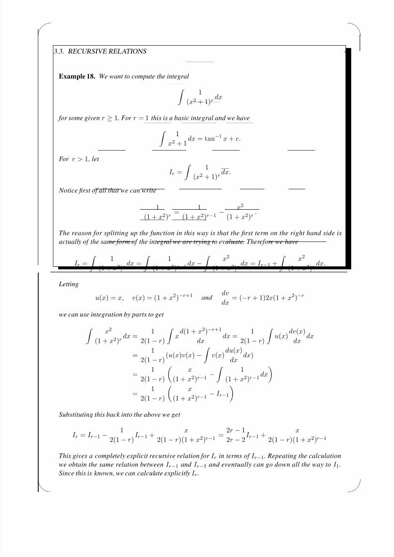
8/6/2019 A 107 Math 2008 Lecture Notes
http://slidepdf.com/reader/full/a-107-math-2008-lecture-notes 41/84
'
&
$
%
3.3. RECURSIVE RELATIONS 41
Example 18. We want to compute the integral
1
(x2 + 1)r dx
for some given r ≥ 1. For r = 1 this is a basic integral and we have
1
x2 + 1dx = tan−1 x + c.
For r > 1 , let
I r =
1
(x2 + 1)rdx.
Notice first of all that we can write
1
(1 + x2)r=
1
(1 + x2)r−1− x2
(1 + x2)r.
The reason for splitting up the function in this way is that the first term on the right hand side is
actually of the same form of the integral we are trying to evaluate. Therefore we have
I r =
1
(1 + x2)rdx =
1
(1 + x2)r−1dx −
x2
(1 + x2)rdx = I r−1 +
x2
(1 + x2)rdx.
Letting
u(x) = x, v(x) = (1 + x2)−r+1 and dvdx
= (−r + 1)2x(1 + x2)−r
we can use integration by parts to get
x2
(1 + x2)rdx =
1
2(1 − r)
x
d(1 + x2)−r+1
dxdx =
1
2(1 − r)
u(x)
dv(x)
dxdx
=1
2(1 − r)(u(x)v(x) −
v(x)
du(x)
dxdx)
=1
2(1 − r)
x
(1 + x2)r−1−
1
(1 + x2)r−1dx
= 12(1 − r)
x
(1 + x2)r−1− I r−1
Substituting this back into the above we get
I r = I r−1 − 1
2(1 − r)I r−1 +
x
2(1 − r)(1 + x2)r−1=
2r − 1
2r − 2I r−1 +
x
2(1 − r)(1 + x2)r−1
This gives a completely explicit recursive relation for I r in terms of I r−1. Repeating the calculation
we obtain the same relation between I r−1 and I r−2 and eventually can go down all the way to I 1.
Since this is known, we can calculate explicitly I r.
8/6/2019 A 107 Math 2008 Lecture Notes
http://slidepdf.com/reader/full/a-107-math-2008-lecture-notes 42/84
'
&
$
%
42 CHAPTER 3. INTEGRALS
3.4 Rational functions
Recall that a rational function of x is a function
f (x)
g(x)
where f, g are polynomials. We want to find f (x)
g(x)dx
Combining some of the methods above we can develop a systematic approach.
3.4.1 Preliminary step: Reducing the degree of the numerator
The first step is to write the rational function as a sum a polynomial and a rational function of x wherethe degree of the numerator is strictly smaller than the degree of the denominator. If deg f < deg gthen we are already in this situation and this step can be skipped. Otherwise we can always write
f = ag + r
where a,g,r are polynomials, and deg r < deg g. Then f (x)
g(x)=
a(x)g(x) + r(x)
g(x)=
a(x) +
r(x)
g(x).
The integral of the polynomial can always be computed and we just need to deal with the situation
in which we have a rational function where the degree of the numerator is strictly smaller than the
degree of the denominator.
Example 19. Suppose f (x) = x3 − 1, g(x) = x + 1 and we want to compute f (x)
g(x)dx =
x3 − 1
x + 1dx.
Then we write
f (x) = x3 − 1 = x2(x + 1) − x2 − 1 = x2(x + 1) − x(x + 1) + x − 1
= x2(x + 1) − x(x + 1) + (x + 1) − 2 = (x2 − x + 1)(x + 1) − 2 = ag + r
where a = x2 − x + 1, r = −2. Then x3 − 1
x + 1dx =
(x2 − x + 1)dx +
−2
x + 2dx
In this particular example we are now in a position to completely solve the integration problem since
we have two integrals which can be computed, Indeed we get (x2 − x + 1)dx =
1
3x3 − 1
2x2 + x
and −2
x + 2dx − 2ln |x + 1| + c
8/6/2019 A 107 Math 2008 Lecture Notes
http://slidepdf.com/reader/full/a-107-math-2008-lecture-notes 43/84
'
&
$
%
3.4. RATIONAL FUNCTIONS 43
3.4.2 Decomposing into partial fractions
We can now assume that we have an integral of the form
f (x)
g(x)dx with deg f < deg g
The next step is to decompose the ratio f (x)/g(x) into partial fractions. More specifically we factorize
g into a product of polynomials of the form x − a and of quadratic factors of the form Q(x) =x2 + bx + c, where Q has no real roots (if it had a real root we could decompose it further into a
product of linear factors). It is then a theorem that f (x)/g(x) is a sum of terms of the form
A
(x − a) pand
Bx + C
[Q(x)]r
where A, B, C are constants and we have to allow every power p and r up to the number of times the
factors x − a and Q(x) respectively, appear in the factorization of g, i.e. the multiplicities of x − aand Q(x).
Example 20.
1
x(x − 1)(x − 2)=
A
x+
B
x − 1+
C
x − 2
Example 21.
1
(x + 1)2
(x2
+ x + 1)2
=A
x + 1
+B
(x + 1)2
+Cx + D
x2
+ x + 1
+Ex + F
(x2
+ x + 1)2
3.4.3 Linear factors
The easiest situation is when the denominator g(x) has all real roots and therefore splits into a product
of linear factors.
Example 22. We want to compute
f (x)
g(x)dx =
x + 1
x2 − x − 12dx.
The denominator splits into two linear factors and so we get
x + 1
x2 − x − 12=
x + 1
(x − 4)(x + 3)=
A
x − 4+
B
x + 3=
A(x + 3) + B(x − 4)
(x − 4)(x + 3)=
(A + B)x + 3A − 4B
(x − 4)(x + 3)
Equating the coefficient of x gives A + B = 1 or A = 1 − B and equating the constant term to get
3A − 4B = 1 and substituting then gives 3 − 3B − 4B = 1 and so B = 2/7 and A = 5/7. Therefore
the integral becomes
x + 1
x2 − x − 12dx =
5/7
x − 4dx +
2/7
x + 3dx =
5
7ln |x − 4| +
2
7ln |x + 3| + const.
8/6/2019 A 107 Math 2008 Lecture Notes
http://slidepdf.com/reader/full/a-107-math-2008-lecture-notes 44/84
'
&
$
%
44 CHAPTER 3. INTEGRALS
If any one of the linear factors appears with higher multiplicity in the decomposition of g then the
partial fraction decomposition of f /g may contain terms with this higher order term on the denomi-
nator. We then always end up with integrals which we can compute, either of the form a
(x + b) pp ≥ 1.
If p = 1 we simply get a
x + b= a ln |x + b| + const.
If p ≥ 2 we get a
(x + b) pdx =
a(x + b)− pdx =
a(x + b)− p+1
(− p + 1)+ const. =
a
(− p + 1)(x + b) p−1+ const.
Example 23. We want to compute 1
(x − 1)2(x + 3).
The decomposition into partial fractions is then
1
(x − 1)2(x + 3)=
A
x + 3+
B
x − 1+
C
(x − 1)2=
A(x − 1)2 + B(x − 1)(x + 3) + C (x + 3)
(x − 1)2(x + 3).
The constants A ,B,C can now be computed in the standard way, multiplying everything out and
equating coefficients. Alternatively, notice that the numerator of the right hand side must add up to
1 for every x. Therefore, letting x = −3 the terms involving B and C vanish and therefore we have
A(x− 1)2 = 16A = 1 and so A = 1/16. Similarly, letting x = 1 the terms involving A and B vanish
and we get C (x + 3) = 4C = 1 and so C = 1/4. To evaluate B notice that if the expression in the
numerator of the right hand side is equal to the expression in the numerator of the left hand side, then
their derivatives must also be equal for every x. The derivative of 1 , the numerator on the left hand
side, is always zero and so the same must be true for the derivative of the expression on the right hand
side. So differentiating with respect to x we must have
d(A(x − 1)2 + B(x − 1)(x + 3) + C (x + 3))
dx= 2A(x − 1) + B(x + 3) + B(x − 1) + C = 0
Evaluating this derivative at x = 1 this gives B(x + 3 + x − 1) + C = 4B + 1/4 = 0 which gives
B = −1/16. Therefore we have
1
(x−
1)2(x + 3)=
1/16
x + 3−
1/16
x−
1+
1/4
(x−
1)2=
1
16ln |x+3|− 1
16ln |x−1|+
1
4(x−
1).
3.4.4 Quadratic factors
It remains to integrate terms of the form Bx + C
[Q(x)]rdx
where Q(x) is a quadratic polynomial with no real roots. In general cannot integrate these terms
directly. However we can simplify them. First of all write
Q(x) = ax2 + bx + c and Q(x) = 2ax + b.
8/6/2019 A 107 Math 2008 Lecture Notes
http://slidepdf.com/reader/full/a-107-math-2008-lecture-notes 45/84
'
&
$
%
3.4. RATIONAL FUNCTIONS 45
Then we can write
Bx + C = α(2ax + b) + β = αQ(x) + β
for some suitable constants α, β This allows us to rewrite the integral as Bx + C
[Q(x)]rdx =
αQ(x) + β
[Q(x)]rdx =
αQ(x)
[Q(x)]rdx +
β
[Q(x)]rdx
The first term can now be integrated directly to get αQ(x)
[Q(x)]r=
α ln[Q(x)] if r = 1α
1−r [Q(x)]1−r if r > 1
The second term is more complicated. We write
Q(x) = (x − γ )2 + β 2 = x2 − 2xγ + γ + β 2
where β is same as before and γ is chosen to make the expression work. Then we let
u =x − γ
β and so x = uβ + γ
which gives therefore β
[Q(x)]rdx =
β
[(x − γ )2 + β 2]rdx =
β
[u2β 2 + β 2]rdx
dudu
=
β
β 2r[u2 + 1]rdx
dudu =
1
β 2r−2
1
[u2 + 1]rrdu
We have therefore reduced the problem to that of computing integrals of the form
1
[x2 + 1]r dx
As described in Example 18, these integrals can be solved recursively.
3.4.5 Rational functions of sin/cos
A rational function consisting of polynomial expressions in sin and cos can be usefully transformed
into a standard rational function substituting
t = tanx
2.
Then we havedt
dx =1
2 sec2 x
2 =1
2 (1 + t2
)
and so
dx =2
1 + t2dt
Notice also that we have
sin x = 2 sinx
2cos
x
2= 2tan
x
2cos2
x
2=
2tan x/2
sec2 x/2=
2t
1 + t2.
and
cos x = cos2x
2− sin2 x
2= cos2
x
2(1 − tan2 x
2) =
1 − t2
1 + t2
8/6/2019 A 107 Math 2008 Lecture Notes
http://slidepdf.com/reader/full/a-107-math-2008-lecture-notes 46/84
'
&
$
%
46 CHAPTER 3. INTEGRALS
Example 24.
1
cos x dx = 1 + t2
1 − t22
1 + t2 dt = 2
1 − t2dt = ln1 + t
1 − t+ c = ln
1 + tan x/2
1 − tan x/2+ c
If integrand involves only tan x or cos2 x or sin2 x, etc. then simply substitute t = tan x. Then
we get dt = sec2 x = (1 + t2)dx
8/6/2019 A 107 Math 2008 Lecture Notes
http://slidepdf.com/reader/full/a-107-math-2008-lecture-notes 47/84
'
&
$
%
Chapter 4
Series
4.1 DefinitionsA series is the sum of the terms of a sequence. So, given a sequence
{t1, t2, t3, . . . , tn}
we define the corresponding series as
t1 + t2 + · · · tn−1 + tn.
Recall the summation notation from Section 1.2.4:
jm=i
tm ≡ ti + ti+1 + ti+2 + · · · + t j.
The index i gives the index on the first term, j gives the index on the last term and the index increases
by 1 each time as you go from term to term. If we have an infinite sequence {u1, u2, u3, . . .} we can,
at least formally, write down the infinite sum
∞i=1
ui = u1 + u2 + u3 + ...
But what does this mean ? How do we sum an infinite number of terms ? We can define the partial
sums
S n = u1 + u2 + ... + un =n
i=1
ui
and use the notion of limit discussed above to ask whether the sequence of partial sums
{S 1, S 2, S 3, . . .}
tends to a finite limit , in which case we say that the sequence converges and write
∞i=1
ui = = limn→∞
S n.
47
8/6/2019 A 107 Math 2008 Lecture Notes
http://slidepdf.com/reader/full/a-107-math-2008-lecture-notes 48/84
'
&
$
%
48 CHAPTER 4. SERIES
Otherwise we say that it diverges. Notice that there are two ways in which an infinite series my
diverge: either by S n → ∞ such as in the example 1 + 1 + 1 + 1 + .... which gives partial sums
S n = n → ∞, or by
S nbeing bounded but simply not converging to any limit, such as in the case
of the series 1 − 1 + 1 − 1 + . . . with partial sums S 1 = 1, S 2 = 0, S 3 = 1, S 4 = 0,... oscillating
between 0 and 1.
Example 25 (Infinite geometric series). Let r ∈ R (notice that r may be negative) and consider the
infinite geometric series
1 + r + r2 + r3 + ... =∞i=0
ri
If |r| < 1 we can find an explicit formula for the partial sums S n = 1+ r+r2+...+rn−1: multiplying
by r:
rS n = r + r2 + r3 + ... + rn−1 + rn
and then
(1 − r)S n = S n − rS n = (1 + r + ... + rn−1) − (r + ...rn) = 1 − rn
so
S n =1 − rn
1 − r
Therefore, if r < 1 we have that rn → 0 as n → ∞ and so
S n → 1
1 − r.
If |r| > 1 then S n → ∞ and so the sequence diverges. If |r| = 1 the formula for the partial sums
is undefined, but in this case we can clearly see that we are in one of the two cases described above:
if r = 1 the series is 1 + 1 + 1 . . . which clearly diverges in the sense that S n → ∞ , if r = −1 the
series is −1 + 1 − 1 + 1 . . . which diverges in the sense that the partial sums S n oscillate between −1and 0 thus do not converge.
4.2 Basic test for non-convergence
We start with a criteria which guarantees that a sequence diverges. Notice that if a sequence converges,
i.e. S n → l, then S n, S n+1 are both very close to l, so S n+1 − S n = (u1 + ... + un + un+1) −(u1 + ... + un) = un+1 must be very small, in fact arbitrarily small if n is large. Thus a necessary
criteria for convergence is that un → 0 as n → ∞ or, in other words,
if un does not tend to 0 then∞n=1
un does not converge.
An intuitive way to see this is that if you are summing up an infinite number of terms each of which has
a given minimum size, the result will clearly be infinite. The only way you can get a finite sum from
an infinite number of terms is if the terms are getting smaller and smaller. It is extremely important to
realize that the non-convergence criterion does not work in the other direction:
un tending to 0 does not imply that
∞n=1
un converges
8/6/2019 A 107 Math 2008 Lecture Notes
http://slidepdf.com/reader/full/a-107-math-2008-lecture-notes 49/84
'
&
$
%
4.3. THE RATIO TEST 49
4.3 The ratio test
It follows from the previous section that un
→0 is a necessary but not sufficient condition for conver-
gence. So, suppose that we have a series for which un → 0. We shall introduce here a fairly general
and very useful test. Consider the series un
and assume that un → 0 for otherwise we would already know that the series diverges. Let
= limn→∞
|un+1||un|
We are supposing here that this limit actually exists. Then
• If l > 1 the series diverges
•If l < 1 the series converges
• If l = 1 the situation is inconclusive (either possibility may occur).
Example 26 (Exponentials ”beat” polynomials). Consider the series
∞n=1
nα
β n
for some α, β > 0. The ratio test gives
|un+1||un| =
(n + 1)α/β n+1
nα/β n=
(n + 1)α
β n+1
β n
nα=
n + 1
n
α 1
β =
1
β
1 +
1
n
α
→ 1
β .
Thus the series diverges if β
∈(0, 1) and converges if β > 1. Notice that this holds for any value of
α. In this particular case it is clear that for β = 1 the terms of the series increase with n and thereforethe series also diverges for β = 1 even though the conclusion does not follow directly from the ratio
test.
Remark 2. It is always important to “test” intuition against formal results. Consider for example the
explicit situation in which β is relatively small and α relatively large in the series defined above. For
example∞n=1
n100
2n=
1
2+
2100
22+
3100
23+
4100
24+ · · ·
Apart from the first term, the others are huge numbers which are in fact increasing very rapidly. The
intuition therefore is that the terms of the series are getting bigger and bigger and surely the series
diverges. What the ratio test easily demonstrates is that this intuition is in fact incorrect. Eventuallythe exponential 2n “catches up” with the term n100 and then quickly becomes much bigger so that
eventually the terms of the series are decreasing quite rapidly and the series converges. If α was
chosen larger, .e.g. α = 1000 and β smaller, e.g. β = 1.01 the effect would be even more dramatic
and it would take longer for the exponential to catch up, but it would eventually, and the series would
still converge.
Exponential growth is very easy to underestimate. There is a famous legend in which some ruler
wants to reward someone for something they have done. He agrees to what seems like a very modest
demand: 1 grain of rice on the first square of a chessboard, 2 on the second, 4 on the third, 8 on the
fourth, then 16, 32..etc., but eventually realizes that not all rice in the entire world would add up to
that much.
8/6/2019 A 107 Math 2008 Lecture Notes
http://slidepdf.com/reader/full/a-107-math-2008-lecture-notes 50/84
'
&
$
%
50 CHAPTER 4. SERIES
Example 27 (Factorials “beat” exponentials). Consider the series
∞n=1
β n
n!
for some β > 0. Then
|un+1||un| =
β n+1/(n + 1)!
β n/n!=
β n+1
β nn!
(n + 1)!=
β
n + 1→ 0
and so the ratio test implies that the series converges for any value of β .
Remark 3. In this example also, it is worth plugging in some explicit numbers to test our intuition.
Choosing some large value of β , e.g. β = 100 we get
∞n=1
100n
n!= 100
1+ 100
2
2+ 100
3
6+ 100
4
24+ · · ·
Once again, the initial terms of the series are increasing very rapidly giving the impression that the
series should diverge. However, the ratio test shows that the series diverges, meaning that the terms
must eventually decrease which implies that the factorial term eventually catches up with and “over-
takes” the exponential term. Indeed, in the exponential term is just 100 we just keep multiplying by
100, whereas in the factorial term you multiply by ever increasing numbers.
Warning: The ratio test requires the limit of the ratios to be less than 1, it is not sufficient for the
ratios themselves to be less than 1.
Example 28. Consider the two series 1
nand
1
n2.
We have respectively
|un+1||un| =
1n+11n
=n
n + 1→ 1 and
un+1
un=
1(n+1)2
1n2
=n
n + 1→ 1
Thus in both cases the ratios tend to 1 and so the ratio test does not allow us to draw any conclusion
as regards the convergence of the series. As we shall see below, the first series diverges whereas the
second converges. We need to develop other tests for these kinds of situations.
4.4 The integral and comparison tests
In some cases we can establish convergence or divergence of a series by comparing the series to one
which we know converges or diverges. Let
an and
bn be two series of positive terms. Suppose
that
an ≤ bn for every n and
bn converges. Then
an converges.
Alternatively, suppose that
an ≥ bn for every n and
bn diverges. Then
an diverges.
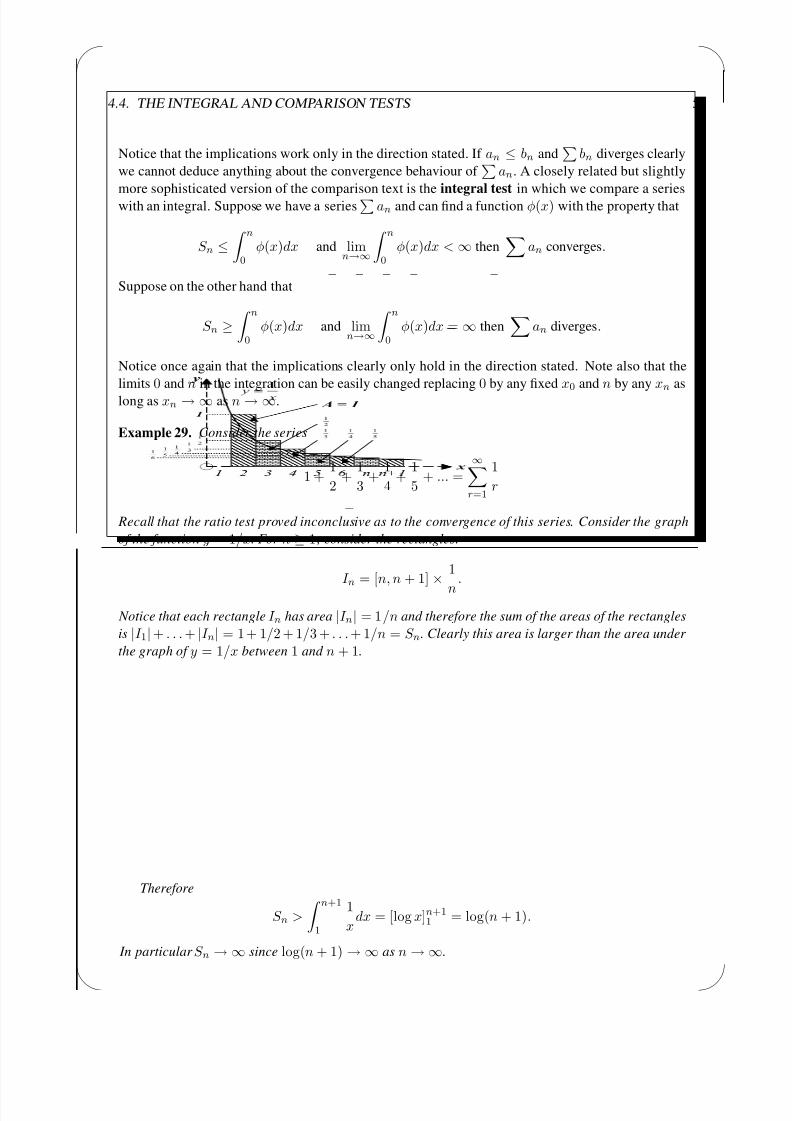
8/6/2019 A 107 Math 2008 Lecture Notes
http://slidepdf.com/reader/full/a-107-math-2008-lecture-notes 51/84
'
&
$
%
4.4. THE INTEGRAL AND COMPARISON TESTS 51
Notice that the implications work only in the direction stated. If an ≤ bn and
bn diverges clearly
we cannot deduce anything about the convergence behaviour of
an. A closely related but slightly
more sophisticated version of the comparison text is the integral test in which we compare a series
with an integral. Suppose we have a series
an and can find a function φ(x) with the property that
S n ≤ n0
φ(x)dx and limn→∞
n0
φ(x)dx < ∞ then
an converges.
Suppose on the other hand that
S n ≥ n0
φ(x)dx and limn→∞
n0
φ(x)dx = ∞ then
an diverges.
Notice once again that the implications clearly only hold in the direction stated. Note also that the
limits 0 and n in the integration can be easily changed replacing 0 by any fixed x0 and n by any xn as
long as xn → ∞ as n → ∞.
Example 29. Consider the series
1 +1
2+
1
3+
1
4+
1
5+ ... =
∞r=1
1
r
Recall that the ratio test proved inconclusive as to the convergence of this series. Consider the graph
of the function y = 1/x. For n ≥ 1 , consider the rectangles:
I n = [n, n + 1]×
1
n.
Notice that each rectangle I n has area |I n| = 1/n and therefore the sum of the areas of the rectangles
is |I 1| + . . . + |I n| = 1 + 1/2 + 1/3 + . . . + 1/n = S n. Clearly this area is larger than the area under
the graph of y = 1/x between 1 and n + 1.
Therefore
S n >
n+1
1
1
xdx = [log x]n+1
1 = log(n + 1).
In particular S n → ∞ since log(n + 1) → ∞ as n → ∞.
8/6/2019 A 107 Math 2008 Lecture Notes
http://slidepdf.com/reader/full/a-107-math-2008-lecture-notes 52/84
'
&
$
%
52 CHAPTER 4. SERIES
4.5 Power Series
A powers series is essentially a series which depends on a fixed set of coefficients{
an
}and a variable
x:∞n=0
anxn = a0 + a1x + a2x2 + ...
Once the coefficients are fixed, we are interested in the convergence or divergence of the series for
different values of x. The set of values of x for which a power series converges is never just some
random or complicated set. Any power series has a radius of convergence, that is, a number R ≥ 0such that the series
converges if |x| < R
diverges if |x| > R.
The case |x| = R may depend on the specific series. If the series converges for all x then we sayR = ∞ Sometimes we want a series in powers of (x − a):
an(x − a)n.
If this is the case, the radius of convergence is R ≥ 0 so that the series
converges if |x − a| < R
diverges if |x − a| > R.
Example 30. Consider the power series
∞n=0
xn = 1 + x + x2 + ...
given by fixing coefficients an ≡ 1. The ratio test gives
limn→∞
|un+1||un| = lim
n→∞
|xn+1
|xn| = |x|
and so the series converges if |x| < 1 , i.e. −1 < x < 1 and diverges if |x| > 1.
Example 31. Consider the power series
∞n=0
xn
n!= 1 + x +
x2
2!+ ...
given by choosing coefficients an = 1/n! Then the ratio between consecutive terms is given by
|un+1||un| =
| xn+1
(n+1)! ||xnn! |
=|xn+1||xn| · n!
(n + 1)!=
|x|n + 1
.
This ratio converges to 0 as n → ∞ for any value of x and therefore the series converges for all x
8/6/2019 A 107 Math 2008 Lecture Notes
http://slidepdf.com/reader/full/a-107-math-2008-lecture-notes 53/84
'
&
$
%
4.6. TAYLOR AND MACLAURIN SERIES 53
4.6 Taylor and Maclaurin Series
4.6.1 Definition
We define the Taylor series of f about the point a to be the power series
f (a) + f (a)(x − a) +f (a)
2(x − a)2 + ...
Using the summation notation we can write this more precisely as
∞n=0
f (n)(a)
n!(x − a)n.
In the special case a = 0 we have
f (0) + f (0)x +f (0)
2x2 + ...
which again we can write more precisely as
f n(0)
n!xn,
and we call this the Maclaurin series.
Remark 4. The Taylor (and Maclaurin) series can always be defined for any function f which can
be differentiated infinitely many times at the points a. Notice that only requires information about f (and all its higher order derivatives) at the point a. As with general power series it is not necessarily
the case that this series converges for all x, and even if it does converge, it is not necessarily the case
that it converges to the precise value f (x). For example, the function
f (x) = e−1/x2
is infinitely differentiable and
f (0)(0) = 0
for all n ≥ 0. Therefore the Taylor series of f is identically 0. However it is not true that the function
itself is identically 0. In general, the convergence of the Taylor series the the correct value f (x) is
a positive answer to the following question: Suppose we know all higher order derivatives of f at a
single point x. Can we calculate the value of f (x) at any other arbitrary point x. In this light it is
really quite remarkable that the taylor series ever converges to the right value at all. The functions for
which the Taylor series does converge to f (x) are called analytic functions, and include all standard
functions such as trigonometric functions, exponentials, logs, and most other functions you are likely
to come across.
Remark 5. In principle there is no reason why a function for which the Taylor series does not converge
to the right value, might not admit a different power series representation which does. In fact this is
not that case. We can show that there is no other power series which could represent the function f .Indeed, suppose that f can be represented as a power series around the point a:
f (x) = a0 + a1(x − a) + a2(x − a)2 + ...
8/6/2019 A 107 Math 2008 Lecture Notes
http://slidepdf.com/reader/full/a-107-math-2008-lecture-notes 54/84
'
&
$
%
54 CHAPTER 4. SERIES
We can show that such a series must necessarily be the Taylor series, i.e. the coefficients must neces-
sarily be of the form
an = f
(n)
(a)n!
Indeed, we must necessarily have a0 = f (a) since the expression must hold for x = a when all terms
vanish except for the a0 term. Differentiating the series terms by term we get
f (x) = a1 + 2a2(x − a) + 3a3(x − a)2 + ...
Again, considering the case x = a this implies that a1 = f (x). Differentiating again we get
f (x) = 2a2 + 6a3(x − a) + ...
and so, letting x = a this gives a2 = f (x)/2. And so on for all terms., Thus, if there is a power
series for f then the Taylor series is it!!!
4.6.2 Computing Taylor series
The Taylor and Maclaurin series of certain functions are very easy to calculate directly from the
definition. It is easy to calculate the Maclaurin series of standard functions
cos x = 1 − x2/2! + x4/4! − x6/6! + · · ·
sin x = x − x3/3! + x5/5! − x7/7! + · · ·
ex
= 1 + x + x2
/2! + x3
/3! + x4
/4! + · · ·and to show that these series converge for all x as power series by using the ratio test.
Example 32. Consider the function f (x) = cos x. Then
f (x) = cos x, f (1)(x) = − sin x, f (2)(x) = − cos x, f (3)(x) = sin x, f (4)(x) = cos x.
The key here is to observe the pattern and notice that f (4) = f and therefore f (5) = f (1) and in
general f (k+4) = f (k). In particular, evaluating the derivatives at x = 0 we have
f (0) = cos 0 = 1, f (1)(0) = − sin 0 = 0, f (2)(0) = − cos0 = −1, f (3)(0) = sin 0 = 0, f (4)(0) = cos 0 = 1, .
Series can be differentiated or integrated term by term.
Example 33. Consider the Maclaurin series
sin x = x − x3
3!+
x5
5!− ...
Differentiating both sides we get
cos x = 1 − x2
2!+
x4
4!− ...
8/6/2019 A 107 Math 2008 Lecture Notes
http://slidepdf.com/reader/full/a-107-math-2008-lecture-notes 55/84
'
&
$
%
4.7. TAYLOR’S THEOREM 55
Example 34. A particularly interesting example is a generalization of the binomial expansion. Let αbe any real number and let
f (x) = (1 + x)α
Differentiating, we get
f (x) = α(1 + x)α−1, f (x) = α(α − 1)(1 + x)α−2
and, in general,
f (n)(x) = α(α − 1)...(α − n + 1)(1 + x)α−n
To calculate the Maclaurin series we evaluate the function and all the derivatives at the point a = 0to get
f (0) = 1, f (0) = α, f (0) = α(α
−1)
and, in general,
f (n)(0) = α(α − 1)...(α − n + 1).
Therefore the Maclaurin series is given by
1 + αx +α(α − 1)
2!x2 + ... +
α(α − 1)...(α − n + 1)
n!xn + · · ·
It is not immediately that this series converges. The ratio test gives
|un+1||un| =
α(α−1)...(α−(n+1)+1)(n+1)! x(n+1)
[α(α−1)...(α−n+1)n! xn]
= α(α
−1)...(α
−n)
α(α − 1)...(α − n + 1) ·n!
(n + 1)! · xn+1xn
=
α − n
n + 1
· |x| =n − α
n + 1· |x| =
1n(n − α)1n(n + 1)
|x| =1 − α
n
1 + αn
· |x| → x
So series converges if |x| < 1 and diverges if |x| > 1. In other words
f (x) = (1 + x)α = 1 + αx +α(α − 1)
2!x2 + ... +
α(α − 1)...(α − n + 1)
n!xn + · · ·
holds true for |x| < 1. Otherwise the series does not converge.
4.7 Taylor’s Theorem
As mentioned above, one of the idea behind Taylor series is that knowledge of more and more higher
order derivatives of f at some given point a yield more and more information about the value of the
function f at other point x different from a. Consider a function f (x) and its Taylor series. Letting
h = x − a, the Taylor series becomes
f (x) = f (a + h) =∞n=0
f (n)(a)
n!hn.
8/6/2019 A 107 Math 2008 Lecture Notes
http://slidepdf.com/reader/full/a-107-math-2008-lecture-notes 56/84
'
&
$
%
56 CHAPTER 4. SERIES
If the series converges, the partial sums of the series converge to the infinite sum as n increases. Let
Rn(h) be the remainder term (error) when we calculate only the first n terms of a series.
f (a + h) = f (a) + f (a)h +f (a)
2!h2 + ... +
f (n−1)(a)
(n − 1)!hn−1 + Rn(h)
=n−1i=0
f (i)(a)
i!hi + Rn(h)
Taylor’s Theorem says that there is some a ≤ x∗ ≤ a + h such that
Rn(h) =f n(x∗)
n!hn.
This can be extremely useful because it can allow us to estimate the error which we make by calculat-
ing the value of a function using only a finite number of terms of the taylor series.
Example 35. For n = 1 , we have
f (x) = f (a + h) = f (a) + R(h)1
and Taylor’s theorem says there exists some x∗ between a and a + h for which
f (a + h) = f (a) + f (x∗) · h
This case follows immediately from the Mean Value Theorem which states that there exists x∗ such
that:
f (x∗) =f (a + h) − f (a)
h
Example 36. Find the first three terms of the Maclaurin expansion of the function f (x) = ln(1 +x) and the form of the remainder term R4. Use the first three terms of the expansion to find an
approximate value for 1x=0
ln(1 + x)
xdx
and use the remainder term R4 to give a bound for the error.
First of all, differentiating f (x) we get
f (x) = (1 + x)−1, f (x) = −(1 + x)−2, f (x) = 2(1 + x)−3, f (x) = −6(1 + x)−4.
Therefore the first terms of the Maclaurin series are
ln(1 + x) = f (x) = f (0) + f (0)x +f (0)x2
2!+
f (x)x3
3!+ R4(x) = x − x2
2+
x3
3+ R4(x)
where
R4(x) =f (x∗)
4!= −6(1 + x∗)−4x4
4!= − x4
4(1 + x∗)4
for some x∗ with 0 ≤ x∗ ≤ x. Notice in particular that for x > 0 the absolute value of R4(x) is
greatest when x∗ = 0 , therefore we get an upper bound for the absolute value
|R4(x)| ≤ x4
4.
8/6/2019 A 107 Math 2008 Lecture Notes
http://slidepdf.com/reader/full/a-107-math-2008-lecture-notes 57/84
'
&
$
%
4.7. TAYLOR’S THEOREM 57
To estimate the integral we write
1x=0
ln(1 + x)
x dx = 10
1
x
x −x2
2 +
x3
3 + R4(x)
dx = 10 1dx−
1
0
x
2 dx+ 10
x
3 dx+ 10
R4(x)
x dx
Integrating the first three terms we get
10
1dx − 10
x
2dx +
10
x
3dx = [x]10 +
x2
4
10
+
x3
9
10
= 1 − 1
4+
1
9=
28
36=
7
9.
So an approximate value for the integral is 1x=0
ln(1 + x)
xdx ≈ 7
9.
But how good is this approximation ? It neglects the last integral which, by Taylor’s Theorem is equalto 1
0
R4(x)
xdx = −
10
x3
4(1 + x∗)4dx = −
x4
16(1 + x∗)4
10
= − 1
16(1 + x∗)4.
for some 0 ≤ x∗ ≤ x. Notice in particular that x∗ is some specific number lying between 0 and
x although we do not know what this number is, since Taylor’s Theorem does not (cannot) specify
its value. However it is clear that the absolute value of the right hand side in the equation above is
decreasing with x∗ and therefore the error cannot be greater in absolute value than the error obtained
by taking x∗ = 0. Thus the absolute value of the maximum error is precisely 1/16. Thus we have
proved that in fact
7
9 ≥ 1
x=0
ln(1 + x)
xdx
≥7
9 −1
16.

8/6/2019 A 107 Math 2008 Lecture Notes
http://slidepdf.com/reader/full/a-107-math-2008-lecture-notes 58/84
'
&
$
%
58CHAPTER 4. SERIES
8/6/2019 A 107 Math 2008 Lecture Notes
http://slidepdf.com/reader/full/a-107-math-2008-lecture-notes 59/84
'
&
$
%
Chapter 5
Limits
5.1 Definition and key properties
The notion of limit is very important in the context of functions. Suppose we have a function f (x).
The we say that
f (x) converges to as x tends to a
and write
f (x) → as x → a or limx→a
f (x) = .
if
limn→∞
f (xn) = for any sequence xn → a with xn = a.
In other words, we are fixing a point a, choosing a sequence xn which converges to a and askingwhether the corresponding values f (xn) converge to (or indeed to anything at all). If we have two
function f, g such that limx→a f (x) and limx→a g(x) both exist, then the limits satisfy the following
key properties (algebra of limits):
1. lim[f (x) ± g(x)] = lim f (x) ± lim g(x)
2. lim[f (x) · g(x)] = lim f (x) · lim g(x)
3. lim[f (x)/g(x)] = lim f (x)/ lim g(x)
5.2 Basic examples
The easiest case is of course, when f (a) is actually defined and f is continuous at the point a.
Example 37. Let f (x) = x3ex + sin(x) , a = 1. Then f (1) is defined and
limx→1
(x3ex + sin(x)) = 13e1 + sin(1) = e + sin(1)
Example 38. Consider
f (x) =x3 + x
x
59
8/6/2019 A 107 Math 2008 Lecture Notes
http://slidepdf.com/reader/full/a-107-math-2008-lecture-notes 60/84
'
&
$
%
60 CHAPTER 5. LIMITS
at a = 0. Then f (a) = 0/0 is not defined. However, for x = 0 we can simplify the expression for
f by dividing top and bottom by x (notice that this can be done only for x = 0). Thus, for x = 0 we
havef (x) = g(x) = x
2
+ 1. Since
f (x) = g(x)for all
x = 0we clearly have
limx→0
x3 + x
x
= lim
x→0(x2 + 1) = 1
Example 39. Calculate
limx→−2
√−2x − 2
x + 2
Notice that for x = −2 the expression is not defined, but for x ≈ −2 and x = −2 it is, including the
term in the square root. Multiplying numerator and denominator by√−2x + 2 and simplifying we
get √−2x − 2
x + 2=
(√−2x − 2)(
√−2x + 2)
(x + 2)(√
−2x + 2)
=−2(x + 2)
(x + 2)(√
−2x + 2)
We then have √−2x − 2
x + 2=
−2√−2x + 2if x = −2.
Notice that we cannot in general simplify by dividing through by x + 2 unless x = −2. Nevertheless,
the equality holds for any x = −2 even very close to −2 and therefore we have
limx→−2
√−2x − 2
x + 2= lim
x→−2
−2√−2x + 2=
−2√4 + 2
= −1
2.
Example 40.
limx→∞
x + 1x
x−
1
x
= limx→∞
1 + 1x2
1−
1
x2
= 1
5.3 Counterexamples
Limits do not necessarily exist at every point and for every function. Recall that the definition of a
limit requires that
f (xn) →
for any sequence xn → a where does not depend on the sequence xn.
Example 41. Consider the function
f (x) = sin1
x.
This function is not defined at x = 0. If 1/x is a multiple of π , i.e. 1/x = nπ for an integer n , thenwe have f (x) = sin 1
x = sin nπ = 0. Therefore there exists a sequence
xn =1
nπ→ 0 such that f (xn) = 0.
On the other hand, if 1/x = nπ + π/2 then f (x) = sin 1x = sin(nπ + π
2 ) = sin π2 = 1. So there
exists a sequence
xn =1
nπ + π/2→ 0 such that f (xn) = 1.
In this example we can find two sequences, both tending to 0, for which the function takes on two
distinct values. Therefore the limit limx→0 f (x) does not exist.
8/6/2019 A 107 Math 2008 Lecture Notes
http://slidepdf.com/reader/full/a-107-math-2008-lecture-notes 61/84
'
&
$
%
5.4. TECHNIQUES FOR CALCULATING LIMITS 61
Sometimes the limit may exist but not coincide with the value of the function at that point.
Example 42. Consider the function
f (x) =
1 if x = 0
−1 if x = 0
Then
f (0) = −1 but limx→0
f (x) = 1.
The property that
limx→a
f (x) = f (a)
is in fact the definition of continuity of f at the point a.
5.4 Techniques for calculating limits
In the examples given so far, the limits can be calculated with some relatively straightforward algebraic
manipulations. However in some cases we need some more sophisticated techniques.
5.4.1 Series expansions
A very powerful technique consist in using the Taylor, Maclaurin or binomial series expansion. The
following example is important and has lots of applications.
Example 43. Compute the following limit:
limx→0
sin(x)x
.
Using the Taylor series of sin we get
limx→0
sin(x)
x= lim
x→0
x − x3
3! + x5
5! − ...
x= lim
x→0
1 − x2
3!+
x4
5!− ...
= 1
Notice that we can only divide through by by x when x = 0. this is sufficient since if the two expres-
sions are equal for all x = 0 their limits as x → 0 must also be equal.
Example 44. Compute the limit
limx→∞x
x2
+ 1 − x2
− 1
This is the product of two functions one of which tends to ∞ and the other one of which tends to 0 as
x → ∞. It is therefore not immediately clear what the product tends to. We can write
x2 + 1 = x2
1
x2+ 1
and therefore
x
x2 + 1 −
x2 − 1
= x
x2
1 +
1
x2
−
x2
1 − 1
x2
= x2
1 +
1
x2−
1 − 1
x2
8/6/2019 A 107 Math 2008 Lecture Notes
http://slidepdf.com/reader/full/a-107-math-2008-lecture-notes 62/84
'
&
$
%
62 CHAPTER 5. LIMITS
Since we are interested in x → ∞ we have 1/x2 → 0 and therefore we can use the binomial expansion
(1 + y)α = 1 + αy +α(α
−1)
2! y2 + ... +α(α
−1)...(α
−n + 1)
n! yn + · · ·
which holds for |y| < 1 to get, letting y = 1/x2 and y = −1/x2
1 +
1
x2=
1 +
1
x2
1/2= 1 +
1
2x2− 1
8x4− 3
48x6− . . .
and 1 − 1
x2=
1 − 1
x2
1/2= 1 − 1
2x2− 1
8x4+
3
48x6− . . .
Subtracting the two series we get
x
x2 + 1 −
x2 − 1
= x2
1
x2+ 1 −
1
x2+ 1
= x2
1
x2− 6
48x4+ ...
= 1 − 1
8x2+ · · ·
Therefore
limx→∞
x
x2 + 1 −
x2 − 1
= limx→∞
[1 − 1
8x2+ · · · ] = 1.
Often we use some basic manipulation and the properties of limits to reduce the function to some-
thing which we can solve using a series expansion.
Example 45. Compute the limit
limθ→0
sin(θ2)
(sin θ)2
We start by writing this expression as a product
sin(θ2)
(sin θ)2=
sin(θ2)
θ2θ2
(sin θ)2
Then we use the algebra of limits to get
limθ→0
sin(θ2)
(sin θ)2 = limθ→0
sin(θ2)
θ2 limθ→0
θ2
(sin θ)2
For the first term we just let x = θ2 and then
limθ→0
sin(θ2)
θ2= lim
x→0
sin x
x= 1.
For the second term we let x = θ and we have
limθ→0
θ2
(sin θ)2= lim
x→0
x
sin x
2= 1.
8/6/2019 A 107 Math 2008 Lecture Notes
http://slidepdf.com/reader/full/a-107-math-2008-lecture-notes 63/84
'
&
$
%
5.4. TECHNIQUES FOR CALCULATING LIMITS 63
5.4.2 Hopital’s rule
A more sophisticated application is ’l’Hopital’s rule which says that if f (a) = 0, g(a) = 0 then
limx→a
f (x)
g(x)= lim
x→a
f (x)
g(x)
If f (a) = 0, g(a) = 0 we can repeat this equation to get
limx→a
f (x)
g(x)= lim
x→a
f (x)
g(x)
and continue until we get some higher order derivative for either f to g which does not vanish, and
whose limit is therefore easy to calculate.
Example 46. Calculate
limx→0
tan2xsinx
Since tan 0 = 0 and sin 0 = 0 we can differentiate numerator and denominator to get
limx→0
tan2x
sinx= lim
x→0
2sec22x
cosx= 2
Example 47. Calculate
limx→0
1 − cosx
x2.
Applying l’Hopital’s rule twice, we get
limx→0
1 − cosxx2
= limx→0
sinx2x
= limx→0
cosx2
= 12
.
Remark 6. L’Hopital’s rule follows immediately from Taylor’s Theorem. Indeed, by Taylor’s theo-
rem, there exist points
a ≤ x∗, x∗∗ ≤ x
such that
f (x) = f (a) + f (a)(x − a) + ... +f (n)(x∗)
n!(x − a)n
and
g(x) = g(a) + g(a)(x
−a) + ... +
g(n)(x∗∗)
n!
(x
−a)n
If f (a) = 0, . . . , f (n−1)(a) = 0, g(a) = 0, . . . , g(n−1)=0 then all terms above vanish except for the
remainder therm and we have
limx→a
f (x)
g(x)= limx→a
f (n)(x∗)
g(n)(x∗∗)= limx→a
f (n)(x)
g(n)(x)
where the second equality follows because a ≤ x∗, x∗∗ ≤ x and thus tend to a as x tends to a.

8/6/2019 A 107 Math 2008 Lecture Notes
http://slidepdf.com/reader/full/a-107-math-2008-lecture-notes 64/84
'
&
$
%
64CHAPTER 5. LIMITS
8/6/2019 A 107 Math 2008 Lecture Notes
http://slidepdf.com/reader/full/a-107-math-2008-lecture-notes 65/84
'
&
$
%
Chapter 6
Partial derivatives
We now try to extend the notion of derivative to functions of several variables. We concentrate on
the two-variable case as the higher variable case is very similar. Suppose f (x, y) is function of two
variables
z = f (x, y)
The graph of this function is a two-dimensional surface in three-dimensional space. How can we
generalize the notion of slope to this higher-dimensional situation ? In some sense we would like to
think of tangent planes to the graph, but how do we represent such tangent planes ? And what good
would they be ?
6.1 Partial derivatives
One way to make sense of derivatives is to fix one of the variables, e.g. x, and thus letting the functiondepend only on the other variable y and thus reducing the situation to the one variable case. Indeed
fixing one variable gives rise to a curve on the graph of f and the slope of this curve is just the
derivative of the one-variable map. We use the notation
∂f
∂xor f x
to denote the partial derivative of f with respect to x, that is, the derivative of the one variable map
which is obtained by fixing the variable y and letting x vary. Similarly, we let
∂f
∂yor f y
denote the partial derivative of f with respect to y.Example 48. Let
f (x, y) = x2y3 + sin(x + 2y) + y.
Then∂f
∂y(x, y) = 3x2y2 + 2 cos(x + 2y) + 1
is the partial derivative of f with respect to y and
∂f
∂y(x, y) = 2y3x + cos(x + 2y) + (0 + 0)
is the partial derivative of f with respect to x.
65
8/6/2019 A 107 Math 2008 Lecture Notes
http://slidepdf.com/reader/full/a-107-math-2008-lecture-notes 66/84
'
&
$
%
66 CHAPTER 6. PARTIAL DERIVATIVES
Remark 7. The partial derivatives f x(x, y) and f y(x, y) associate tangent lines to the graph of f (x, y)at the point ((x,y ,f (x, y)). These two lines span a two-dimensional plane T (x, y). This is called the
tangent plane to the graph. Although it is non-trivial, it is true that any line tangent at the point
(x,y ,f (x, y)) to any curve γ on the graph of f , through the point (x,y ,f (x, y)) also lies in this
tangent plane. Therefore one could in principle calculate it by taking directional derivatives in any
direction, not necessarily along the coordinate axes.
6.2 Higher order partial derivatives
The partial derivatives of f are themselves functions of both variables x and y. Therefore to differen-
tiate them we also need to consider their own partial derivatives. We let
∂ 2
f ∂x2 = f xx = ∂
∂f
∂x∂x
and ∂ 2
f ∂y2 = f yy =
∂ ∂f
∂y∂y
denote the second order partial derivative of f with respect to x and y respectively. We let
∂ 2f
∂x∂y= f xy =
∂ ∂f ∂x
∂y
denote the second order mixed partial derivative of f with respect to y, i.e. the partial derivative with
respect to y of the partial derivative with respect to y. In general we have
f xy = f yx.
6.3 Functions of more than 2 variables
Suppose we have a function
V (x,y ,z)
of three (or more) variables. Then we can argue exactly as above and define the partial derivatives in
a certain direction by fixing all but one of the variables ad considering the derivative of the function
as only that one variable is varied. Thus we define the partial derivatives
∂V
∂x= V x
∂V
∂y= V y
∂V
∂z= V z
Example 49. Let V (x,y,z) =
x + y2 + z3. The the partial derivative with respect to x is given
by
V x =1
2
x + y2 + z3.
The partial derivatives V y and V z and the higher order derivatives can then be calculated correspond-
ingly.
8/6/2019 A 107 Math 2008 Lecture Notes
http://slidepdf.com/reader/full/a-107-math-2008-lecture-notes 67/84
'
&
$
%
6.4. ESTIMATING SMALL CHANGES IN TWO OR MORE VARIABLES 67
6.4 Estimating small changes in two or more variables
Similar estimates can be carried out in the two variable situation. Suppose we have a function
f (x, y)
of two variables. We let δx denote a small change in the x variable, and δy a small change in the yvariable. We want to estimate
δf = f (x + δx,y + δy) − f (x, y)
Using the one variable case we can write
δf = f (x + δx,y + δy) − f (x, y + δy) + f (x, y + δy) − f (x, y) ≈ δf
δxδx +
δf
δyδy
Example 50. A(x, y) = xy area of rectangle side x and y. Sides change from x: 2 to 2.01cm, y: 3
to 3.02cm.
δA ≈ δA
δxδx +
δA
δyδy = yδx + xδy = 3 · 0.01 + 2 · 0.02 = 0.07cm2
6.5 Chain rule for two variables
For function of two or more variables we have three different cases.
A function of one variable depending on several variables:
Suppose we have a functionf (u(x,y,...))
where f depends on the single variable u and u depends on several variables x , y , . . .. Then, a small
change in one of the variable, say x, variable is estimated exactly as in the 1 variable case, by
δf
δx≈ df
du
δu
δx
and, taking the limits,df
dx=
df
du
du
dx,
and similarly in the other variables.
A function of several variables each depending on a single variable
Suppose we have a function
f (x(t), y(t))
of two variables,s x, y each depending on the same variable t. We want the derivative of f with respect
to t. Clearly varying t affects the other variables which all affect the value of f . So if δt represents a
small change in t, using the one variable case, we have
δx ≈ dx
dtδt and δy ≈ dy
dtδt
8/6/2019 A 107 Math 2008 Lecture Notes
http://slidepdf.com/reader/full/a-107-math-2008-lecture-notes 68/84
'
&
$
%
68 CHAPTER 6. PARTIAL DERIVATIVES
and therefore
δf ≈ δf
δxδx +
δf
δyδy ≈ δf
δx
dx
dtδt +
δf
δy
dy
dtδt
orδf
δt≈ δf
δx
dx
dtδt +
δf
δy
dy
dt
Once again, since δf/δx converges to df/dx this gives
df
dt=
df
dx
dx
dt+
df
dy
dy
dt.
The case of a function
f (x(t), x(t), z(t),...)
of several variables, each of which depends on a single variable t is treated in exactly the same way
and gives
df dt
= df dx
dxdt
+ df dy
dydt
+ df dz
dzdt
+ ...
Example 51. Let
A(x(t), y(t)) = xy = x(t)y(t)
be the area of rectangle with sides of length length x(t), y(t) (changing with t). Suppose that for some
t , x(t) = 2, y(t) = 3 , and x is increasing at 1cm/sec and y is decreasing at 0.5cm/sec. How fast is
A changing?
dA
dt=
δA
δx
dx
dt+
δA
δy
dy
dt= y
dx
dt+ x
dy
dt= 3 · 1 + 2(−0.5) = 3 − 1 = 2
A is increasing by 2cm2
/sec
Functions of several variables each depending on several variables
The most complicated case is that in which we have a function
f (x, y)
where each of the two variables
x = x(u, v), y = y(u, v)
depend on further two variables u, v. Then f (x(u, v), y(u,v, )) is effectively a function of the two
variables u and v and we need to talk about the partial derivatives of f with respect to u and v. By
using the same arguments as above we get
df
du=
df
dx
dx
du+
df
dy
dy
du
anddf
dv=
df
dx
dx
dv+
df
dy
dy
dv.
Example 52. Suppose that x = u2 + v2 and y = u2 − v2. Then, for any function f (x, y) we have
δf
δu=
δf
δx2u +
δf
δy2u and
δf
δv=
δf
δx2v +
δf
δy2v
8/6/2019 A 107 Math 2008 Lecture Notes
http://slidepdf.com/reader/full/a-107-math-2008-lecture-notes 69/84
'
&
$
%
6.5. CHAIN RULE FOR TWO VARIABLES 69
The situation (x(u, v), y(u, v)) can be thought of as a change of coordinates in the plane. For
example the change of coordinates between Cartesian and Polar coordinates is given by
x = rcosθ and y = rsinθ
Given any function f (x, y) one can find formulae expressing ∂f ∂r and ∂f
∂θ in terms of ∂f ∂x and ∂f ∂y (see
Exercise Sheet).

8/6/2019 A 107 Math 2008 Lecture Notes
http://slidepdf.com/reader/full/a-107-math-2008-lecture-notes 70/84
'
&
$
%
70CHAPTER 6. PARTIAL DERIVATIVES
8/6/2019 A 107 Math 2008 Lecture Notes
http://slidepdf.com/reader/full/a-107-math-2008-lecture-notes 71/84
'
&
$
%
Chapter 7
Graphs
Sometimes it is difficult to make precise quantitative calculations of specific functions, and easier to
obtain some basic qualitative description of the function by identifying basic geometrical features of
its graph.
7.1 Functions of one variable
We start with a one-variable function
y = f (x)
7.1.1 Asymptotes
A first basic characteristic of f is the existence of any vertical asymptotes, i.e. points x at whichf (x) = ±∞ e.g. if denominator is zero. By considering the sign of f near the asymptotes it is
possible to start sketching the graph.
Example 53. The function
y =1
x − 1
has a vertical asymptote at x=1. Moreover, f (x) > 0 if x > 1 and f (x) < 0 if x < 1.
1
A second important feature is the behaviour for large x. In many cases you
get a horizontal asymptote.
Example 54. The function
y = f (x) =1
x − 1
has a horizontal asymptote at y =0. As x gets larger and larger in the positive
direction f (x) gets smaller and smaller but remains positive, as x gets larger
and larger in the negative direction, f (x) gets smaller and smaller in modulus,
but remains negative.
Is is also possible to have oblique asymptotes.
71
8/6/2019 A 107 Math 2008 Lecture Notes
http://slidepdf.com/reader/full/a-107-math-2008-lecture-notes 72/84
'
&
$
%
72 CHAPTER 7. GRAPHS
Example 55. The function
y = f (x) = x +1
xhas an asymptote of slope 1. As |x| gets larger and larger, the value of f (x) gets closer and closer to
1. Moreover f (x) > 0 when x > 0 and f (x) < 0 when x < 0. It also has an asymptote at 0.
7.1.2 The sign of the derivative
1
Information about asymptotes and the behaviour of f (x) when x is large gives
precisely that, it is then up to us to join these sections of the graph. In simple
cases the graph is essentially monotone, at least in each section, and joining the
regions is quite intuitive. However this is not always the case (in principle the
graph could be very wiggly) and we need a more systematic way of understand-
ing the shape of the graph away from asymptotes.The derivative f (x) of the function gives information about the slope of the
graph at various points, and we can use this information to complete the sketch.
In particular,
f is increasing if f > 0, decreasing if f < 0 and horizontal if
f = 0.
Example 56. In the example above,
y = f (x) = x +1
xwe have
f (x) = 1 − 1
x2
and so
f (x) = 0 if 1 − 1
x2= 0, i.e. x = ±1.
Also, f (x) > 0 and so the slope of the graph is increasing between x = −1 and x = +1 and
f (x) < 0 and the the slope of the graph is decreasing everywhere else. This now gives sufficient
information to draw an essentially correct graph of the function.
Example 57. Consider the function
y = f (x) =x + 2
x2 − x + 2=
x + 2
(x − 2)(x + 1).
We have vertical asymptotes at x = 2 and x = −1. Moreover, f (x) > 0 for x > 2 and x < −1 and
f (x) < 0 for −1 < x < 2. To study the behaviour for large |x| divide numerator and denominator
by x2 (this is possible to do whenever x = 0) to get
y =(x + 2)/x2
(x2 − x − 2)/x2=
1x + 2
x2
1 − 1x − 2
x2
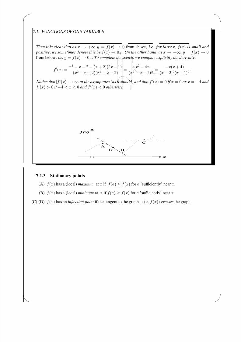
8/6/2019 A 107 Math 2008 Lecture Notes
http://slidepdf.com/reader/full/a-107-math-2008-lecture-notes 73/84
'
&
$
%
7.1. FUNCTIONS OF ONE VARIABLE 73
Then it is clear that as x → +∞ y = f (x) → 0 from above , i.e. for large x , f (x) is small and
positive, we sometimes denote this by f (x) → 0+. On the other hand, as x → −∞ , y = f (x) → 0from below , i.e.
y = f (x) → 0−. To complete the sketch, we compute explicitly the derivative
f (x) =x2 − x − 2 − (x + 2)(2x − 1)
(x2 − x − 2)(x2 − x − 2)=
−x2 − 4x
(x2 − x − 2)2=
−x(x + 4)
(x − 2)2(x + 1)2.
Notice that |f (x)| → ∞ at the asymptotes (as it should) and that f (x) = 0 if x = 0 or x = −4 and
f (x) > 0 if −4 < x < 0 and f (x) < 0 otherwise.
7.1.3 Stationary points
(A) f (x) has a (local) maximum at x if f (a) ≤ f (x) for a ’sufficiently’ near x.
(B) f (x) has a (local) minimum at x if f (a) ≥ f (x) for a ’sufficiently’ near x.
(C)-(D) f (x) has an inflection point if the tangent to the graph at (x, f (x)) crosses the graph.
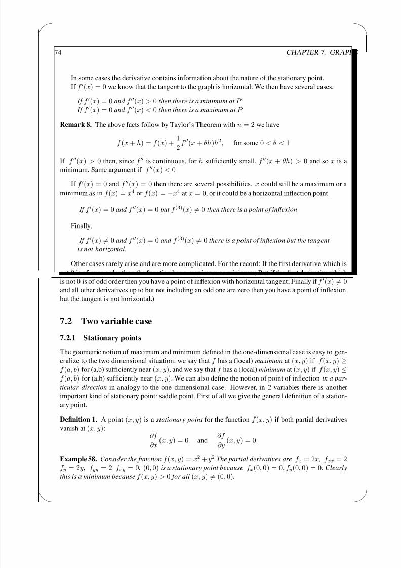
8/6/2019 A 107 Math 2008 Lecture Notes
http://slidepdf.com/reader/full/a-107-math-2008-lecture-notes 74/84
'
&
$
%
74 CHAPTER 7. GRAPHS
In some cases the derivative contains information about the nature of the stationary point.
If f (x) = 0 we know that the tangent to the graph is horizontal. We then have several cases.
If f (x) = 0 and f (x) > 0 then there is a minimum at P If f (x) = 0 and f (x) < 0 then there is a maximum at P
Remark 8. The above facts follow by Taylor’s Theorem with n = 2 we have
f (x + h) = f (x) +1
2f (x + θh)h2, for some 0 < θ < 1
If f (x) > 0 then, since f is continuous, for h sufficiently small, f (x + θh) > 0 and so x is a
minimum. Same argument if f (x) < 0
If f (x) = 0 and f (x) = 0 then there are several possibilities. x could still be a maximum or a
minimum as in f (x) = x4 or f (x) =
−x4 at x = 0, or it could be a horizontal inflection point.
If f (x) = 0 and f (x) = 0 but f (3)(x) = 0 then there is a point of inflexion
Finally,
If f (x) = 0 and f (x) = 0 and f (3)(x) = 0 there is a point of inflexion but the tangent
is not horizontal.
Other cases rarely arise and are more complicated. For the record: If the first derivative which is
not 0 is of even order then the function has a maximum or minimum; But if the first derivative which
is not 0 is of odd order then you have a point of inflexion with horizontal tangent; Finally if f (x) = 0and all other derivatives up to but not including an odd one are zero then you have a point of inflexion
but the tangent is not horizontal.)
7.2 Two variable case
7.2.1 Stationary points
The geometric notion of maximum and minimum defined in the one-dimensional case is easy to gen-
eralize to the two dimensional situation: we say that f has a (local) maximum at (x, y) if f (x, y) ≥f (a, b) for (a,b) sufficiently near (x, y), and we say that f has a (local) minimum at (x, y) if f (x, y) ≤f (a, b) for (a,b) sufficiently near (x, y). We can also define the notion of point of inflection in a par-
ticular direction in analogy to the one dimensional case. However, in 2 variables there is another
important kind of stationary point: saddle point. First of all we give the general definition of a station-ary point.
Definition 1. A point (x, y) is a stationary point for the function f (x, y) if both partial derivatives
vanish at (x, y):∂f
∂x(x, y) = 0 and
∂f
∂y(x, y) = 0.
Example 58. Consider the function f (x, y) = x2 + y2 The partial derivatives are f x = 2x , f xx = 2f y = 2y , f yy = 2 f xy = 0. (0, 0) is a stationary point because f x(0, 0) = 0, f y(0, 0) = 0. Clearly
this is a minimum because f (x, y) > 0 for all (x, y) = (0, 0).
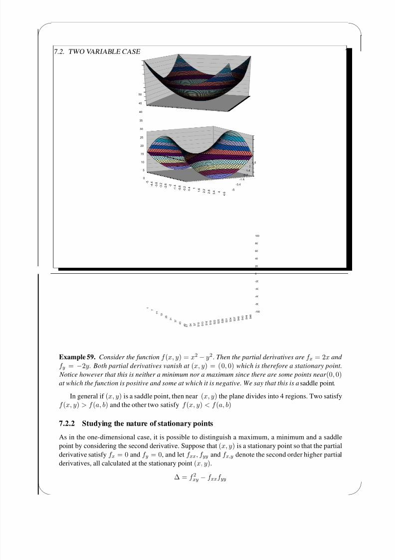
8/6/2019 A 107 Math 2008 Lecture Notes
http://slidepdf.com/reader/full/a-107-math-2008-lecture-notes 75/84
'
&
$
%
7.2. TWO VARIABLE CASE 75
- 5
- 4 .
4
- 3 .
8
- 3 .
2
- 2 .
6 - 2
- 1 .
4
- 0 .
8
- 0 .
2
0 .
4 1
1 .
6
2 .
2
2 .
8
3 .
4 4
4 .
6
-5
-3.4
-1.8
-0.2
1.4
3
4.6
0
5
10
15
20
25
30
35
40
45
50
1
7
1 3
1 9
2 5
3 1
3 7
4 3
4 9
S 1
S 4
S 7
S 1 0
S 1 3
S 1 6
S 1 9
S 2 2
S 2 5
S 2 8
S 3 1
S 3 4
S 3 7
S 4 0
S 4 3
S 4 6
S 4 9
-100
-80
-60
-40
-20
0
20
40
60
80
100
Example 59. Consider the function f (x, y) = x2 − y2. Then the partial derivatives are f x = 2x and
f y = −2y. Both partial derivatives vanish at (x, y) = (0, 0) which is therefore a stationary point.
Notice however that this is neither a minimum nor a maximum since there are some points near (0, 0)at which the function is positive and some at which it is negative. We say that this is a saddle point.
In general if (x, y) is a saddle point, then near (x, y) the plane divides into 4 regions. Two satisfy
f (x, y) > f (a, b) and the other two satisfy f (x, y) < f (a, b)
7.2.2 Studying the nature of stationary points
As in the one-dimensional case, it is possible to distinguish a maximum, a minimum and a saddle
point by considering the second derivative. Suppose that (x, y) is a stationary point so that the partial
derivative satisfy f x = 0 and f y = 0, and let f xx, f yy and f x,y denote the second order higher partial
derivatives, all calculated at the stationary point (x, y).
∆ = f 2xy − f xxf yy
8/6/2019 A 107 Math 2008 Lecture Notes
http://slidepdf.com/reader/full/a-107-math-2008-lecture-notes 76/84
'
&
$
%
76 CHAPTER 7. GRAPHS
Then, if ∆ > 0 then (x, y) is a saddle point. If ∆ < 0 then (a, b) is: a maximum if f xx(a, b) < 0and a minimum if f xx(a, b) > 0.
Example 60. Consider the function
f (x, y) = x2y − y +1
2y2
To find the stationary points we compute the first order partial derivatives and set them equal to zero.
Thus we have
f x = 2xy = 0 ⇔ xy = 0 ⇔ x = 0 or y = 0
So the partial derivative with respect to x vanishes whenever x = 0 or y = 0. In particular any
stationary point must lie on one of the two coordinate axes. Notice that this simplifies our calculation
for the zeroes of the partial derivatives with respect to y. Indeed we have
f y = x2 − 1 + y = 0
If x = 0 then
f y = −1 + y = 0 ⇔ y = 1
and if y = 0 then
f y = x2 − 1 = 0 ⇔ x2 = 1 ⇔ x = ±1
Therefore there are three stationary points: (0, 1), (1, 0) and (−1, 0) To determine what type of sta-
tionary point they are, we calculate the second order partial derivatives:
f xx = 2y. f xy = 2x, f yy = 1.
Therefore
∆(0, 1) = −2, ∆(1, 0) = 4, ∆(−1, 0) = 4
corresponding to a minimum at (0, 1) since f xx(0, 1) > 0 and two saddle points at (1, 0) and (−1, 0).
7.3 Contour sketching
The graph of a function of two variables is a surface in three-dimensional space and is therefore quite
difficult to sketch. One way to visualize the graph is to sketch contour lines, i.e. curves f (x, y) = cfor various constants c. This is like slicing the surface with a horizontal plane z = c, projecting back
onto xy plane.
Basic examples
Example 61. Consider the function
f (x, y) = x2 + y2
discussed above, which has a minimum at (0, 0). Then the contour lines are given by a family of
concentric circles
f (x, y) = x2 + y2 = c
parametrized by c. Notice that this equation has no solution for c < 0 corresponding to the fact that
a horizontal slice through z = c does not intersect the graph of f .
8/6/2019 A 107 Math 2008 Lecture Notes
http://slidepdf.com/reader/full/a-107-math-2008-lecture-notes 77/84
'
&
$
%
7.3. CONTOUR SKETCHING 77
Example 62. Consider the function
f (x, y) = x2 − y2
which has a saddle point at (0, 0). Then, for each c = 0 , the contour lines are given two hyperbolasobtained as solutions to the equation
x2 − y2 = c.
General theory
How to sketch contour lines:
1. Solve f x = 0, f y = 0 to find stationary points.
2. Classify them as max/min/saddle.
3. Calculate the values f (x, y) of f at the stationary points. Draw contours passing through saddle
points.
4. Sketch the other contours using the following principle:
(a) near max or min they look like concentric circles
(b) near saddle point they have four sections as outlined in example
(c) qualitatively they do not change as c goes from one stationary point to the other
Example 63. Consider the function
f (x, y) = x2y − y +1
2y2
By calculating partial derivatives we find stationary points: (0, 1)−mininum, (1, 0)−saddle, (−1, 0)−saddle. We then calculate the value of f at stationary points, i.e. the height of the graph above these
points. We have
f (0, 1) = −1
2, f (1, 0) = 0, f (−1, 0) = 0.
We then draw the contour lines corresponding to slicing the graph at the level of the saddle points,
i.e. c = 0 , we have to solve
y(x2 − 1 +1
2y) = 0.
The solutions are y = 0 or y = 2(1 − x2) Thus the contour lines through the saddle points
consist of the x-axis and an inverted parabola. See picture on next page.
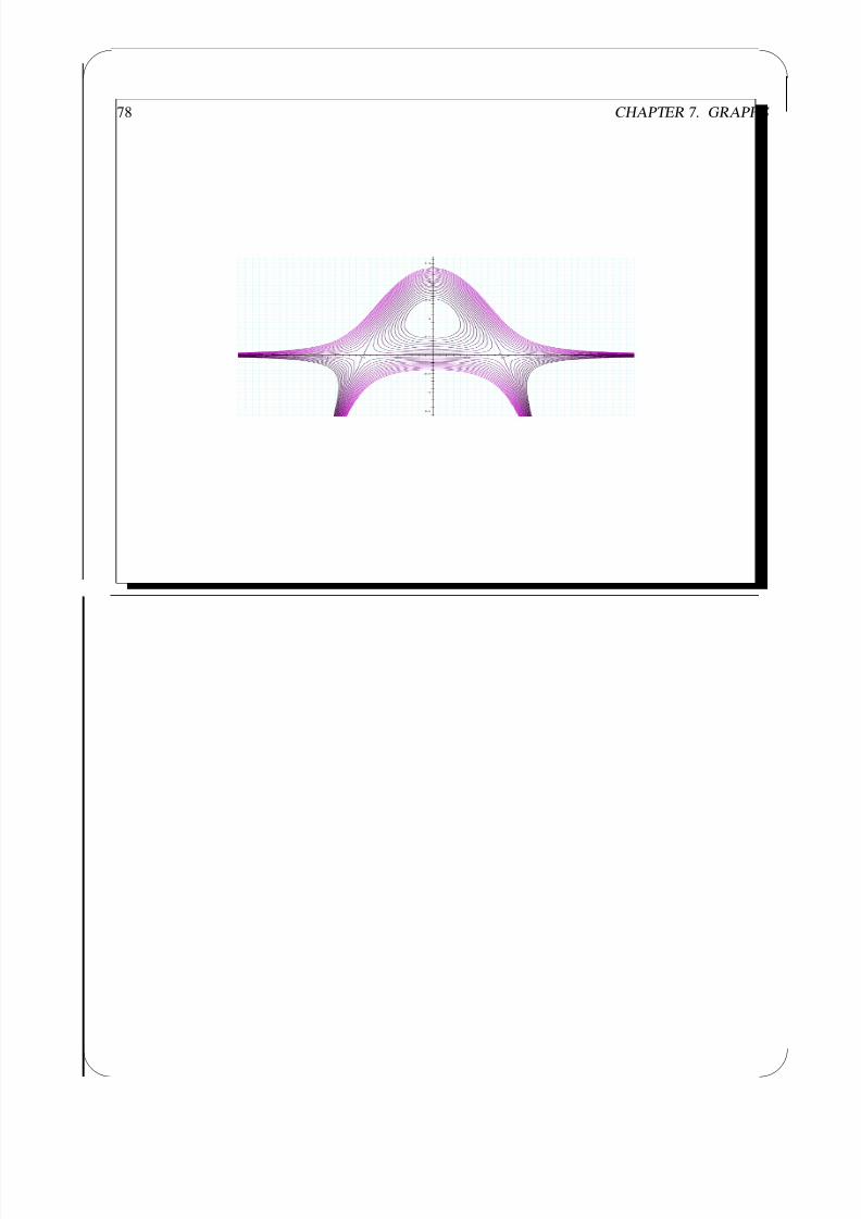
8/6/2019 A 107 Math 2008 Lecture Notes
http://slidepdf.com/reader/full/a-107-math-2008-lecture-notes 78/84
'
&
$
%
78 CHAPTER 7. GRAPHS
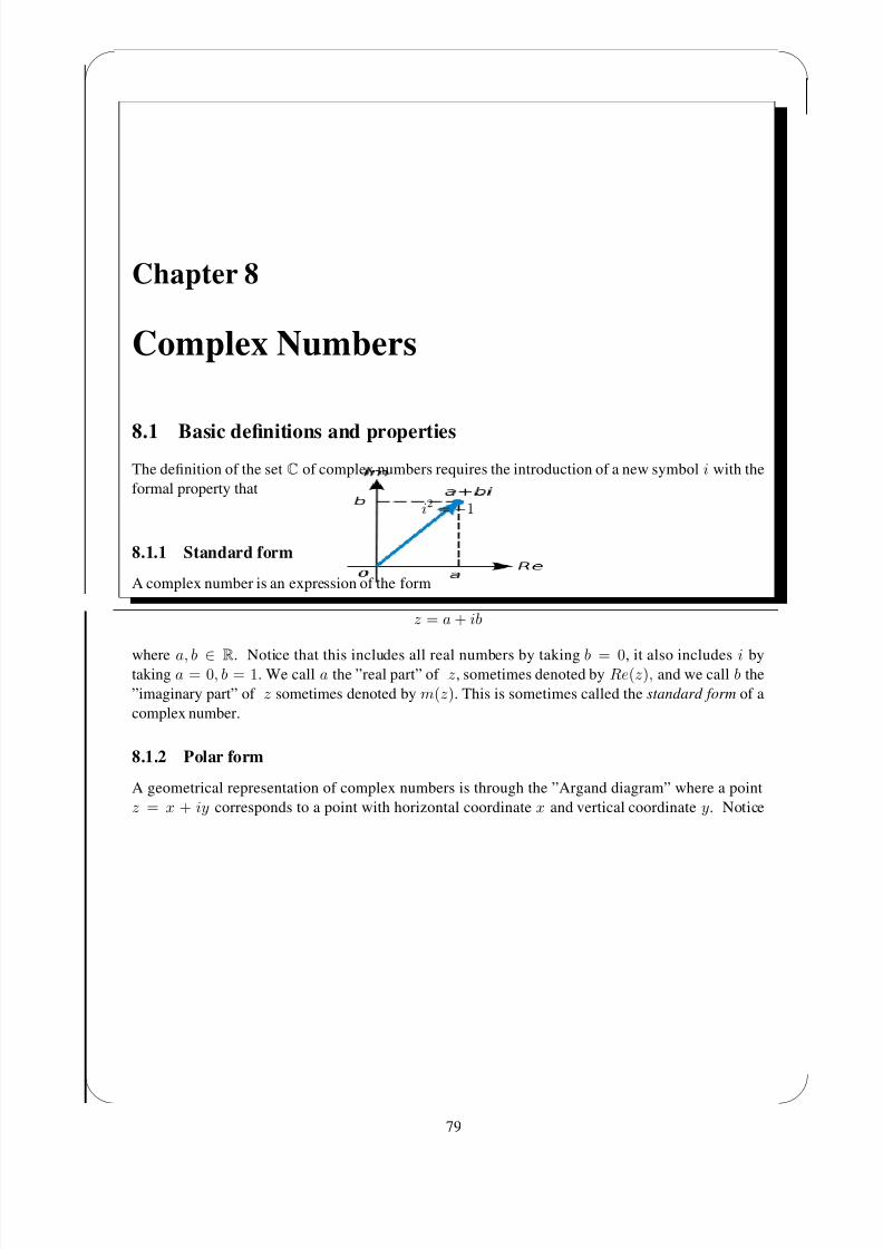
8/6/2019 A 107 Math 2008 Lecture Notes
http://slidepdf.com/reader/full/a-107-math-2008-lecture-notes 79/84
'
&
$
%
Chapter 8
Complex Numbers
8.1 Basic definitions and propertiesThe definition of the set C of complex numbers requires the introduction of a new symbol i with the
formal property that
i2 = −1
8.1.1 Standard form
A complex number is an expression of the form
z = a + ib
where a, b ∈ R. Notice that this includes all real numbers by taking b = 0, it also includes i bytaking a = 0, b = 1. We call a the ”real part” of z, sometimes denoted by Re(z), and we call b the
”imaginary part” of z sometimes denoted by m(z). This is sometimes called the standard form of a
complex number.
8.1.2 Polar form
A geometrical representation of complex numbers is through the ”Argand diagram” where a point
z = x + iy corresponds to a point with horizontal coordinate x and vertical coordinate y. Notice
79

8/6/2019 A 107 Math 2008 Lecture Notes
http://slidepdf.com/reader/full/a-107-math-2008-lecture-notes 80/84
'
&
$
%
80 CHAPTER 8. COMPLEX NUMBERS
that according to the definition of complex numbers each complex number corresponds to a unique
point and vice versa the each point corresponds to a unique complex number. This representation of
complex numbers allows us to write complex numbers in polar form: each complex numberz = x+iycan be written as
z = r(cosθ + isinθ)
where
r = |z| =
x2 + y2 and θ = tan−1(y/x).
r is called the modulus of z, and θ is called the argument of z and often denoted by Arg(z).
8.1.3 Exponential form
A third, very useful way of writing complex numbers is a consequence of Euler’s formula which is
eiθ = cos θ + i sin θ.
Then we can write
z = r(cos θ + i sin θ) = reiθ.
This is sometimes called the exponential form of a complex number.
8.1.4 Arithmetic operations
We can define a consistent arithmetic of complex numbers in the following way. Let z = x + iy and
w = u + iv, be two complex numbers. Then we define addition by
z + w = (x + u) + i(y + v)
and multiplication by
zw = (x + iy)(u + iv) = xu + iyu + xiv + i2yv = (xu − yv) + i(yu + xv)
Addition and multiplication satisfy the usual commutative and distributive properties:
zw = wz,z(w + y) = zw + zy
, etc. In order to define division is is sufficient to define the inverse 1/z of a complex number z (since
division is just multiplication by the inverse). Notice that 1/z = 1/x + iy is not formally a complex
number in the sense that it does no have the form stated above. However, by a standard procedure, we
can calculate the inverse by multiplying numerator and denominator by x − iy (sometimes called the
conjugate of z = x + iy) and using the standard equality (a + b)(a − b) = a2 − b2:
1
x + iy=
1
x + iy
x − iy
x − iy=
x − iy
(x + iy)(x − iy)=
x + iy
x2 − i2y2=
x + iy
x2 + y2=
x
x2 + y2+ i
y
x2 + y2.
Example 64. if z = 2 + 3i , we have
1
2 + 3i=
1
2 + 3i
(2 − 3i)
(2 − 3i)=
2 − 3i
13=
2
13+ i
3
13
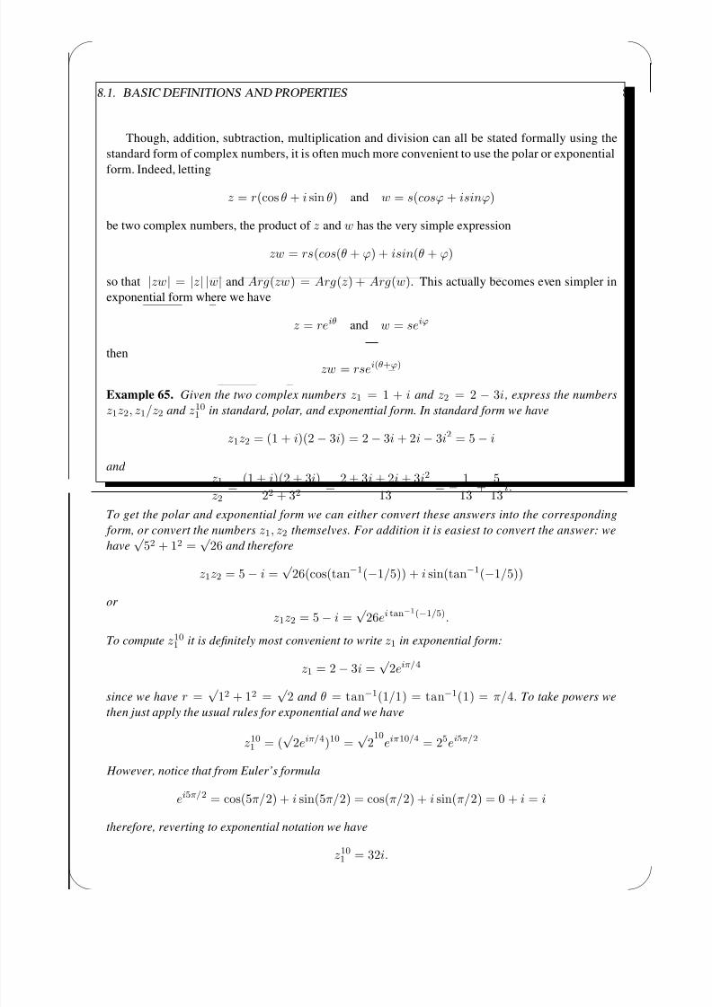
8/6/2019 A 107 Math 2008 Lecture Notes
http://slidepdf.com/reader/full/a-107-math-2008-lecture-notes 81/84
'
&
$
%
8.1. BASIC DEFINITIONS AND PROPERTIES 81
Though, addition, subtraction, multiplication and division can all be stated formally using the
standard form of complex numbers, it is often much more convenient to use the polar or exponential
form. Indeed, letting
z = r(cos θ + i sin θ) and w = s(cosϕ + isinϕ)
be two complex numbers, the product of z and w has the very simple expression
zw = rs(cos(θ + ϕ) + isin(θ + ϕ)
so that |zw| = |z| |w| and Arg(zw) = Arg(z) + Arg(w). This actually becomes even simpler in
exponential form where we have
z = reiθ and w = seiϕ
thenzw = rsei(θ+ϕ)
Example 65. Given the two complex numbers z1 = 1 + i and z2 = 2 − 3i , express the numbers
z1z2, z1/z2 and z101 in standard, polar, and exponential form. In standard form we have
z1z2 = (1 + i)(2 − 3i) = 2 − 3i + 2i − 3i2 = 5 − i
and z1z2
=(1 + i)(2 + 3i)
22 + 32=
2 + 3i + 2i + 3i2
13= − 1
13+
5
13i.
To get the polar and exponential form we can either convert these answers into the corresponding
form, or convert the numbers z1, z2 themselves. For addition it is easiest to convert the answer: wehave
√52 + 12 =
√26 and therefore
z1z2 = 5 − i =√
26(cos(tan−1(−1/5)) + i sin(tan−1(−1/5))
or
z1z2 = 5 − i =√
26ei tan−1(−1/5).
To compute z101 it is definitely most convenient to write z1 in exponential form:
z1 = 2 − 3i =√
2eiπ/4
since we have r =√
12 + 12 =√
2 and θ = tan−1(1/1) = tan−1(1) = π/4. To take powers we
then just apply the usual rules for exponential and we have
z101 = (√
2eiπ/4)10 =√
210
eiπ10/4 = 25ei5π/2
However, notice that from Euler’s formula
ei5π/2 = cos(5π/2) + i sin(5π/2) = cos(π/2) + i sin(π/2) = 0 + i = i
therefore, reverting to exponential notation we have
z101 = 32i.
8/6/2019 A 107 Math 2008 Lecture Notes
http://slidepdf.com/reader/full/a-107-math-2008-lecture-notes 82/84
'
&
$
%
82 CHAPTER 8. COMPLEX NUMBERS
8.1.5 Geometrical properties
The fact that complex numbers “live” on the plane instead of the line gives them a much richer ge-
ometry that that of the real numbers. It is very useful to try to have a geometric picture in your head
when solving certain equations involving complex numbers, even though the calculations may be
completely analytical.
Example 66. Describe the regions in the complex plane where |z2| = 5|z|. Recall that |z| is just the
distance of the point z from the origin and therefore |z2| = |z|2. Therefore the equation is the same
as |z|2 = 5|z|. z = 0 (the origin) is clearly a solution and, for z = 0 we can divide through to get
|z| = 5 which is the circle of radius 5.
Example 67. Describe the region in the complex plane where |z −i| > |z + 1|. Writing z = x+ iy we
have z
−i = x + (y
−1)i and z + i = x + (y + 1)i. Moreover
|z
|= x2 + y2 and so
|z
−i
|>
|z + i
|is equivalent to x2 + (y − 1)2 >
x2 + (y + 1)2.
Thus this is satisfied if and only if
(y − 1)2 > (y + 1)2
which is like saying the y has to be closer to −1 than it is to y. It is therefore equivalent to the
condition y < 0. The geometric locus is therefore the set of all point z = x + iy with y < 0 , i.e. the
lower half plane.
8.2 De Moivre’s Theorem
Using polar coordinates and the expression given above for the multiplication of complex numbers
we get
zn = [r(cosθ + isinθ]n = rn[cos(nθ) + isin(nθ)]
In particular, for r = 1, i.e. for a complex number on the unit circle, this gives De Moivre’s Theorem:
(cosθ + isinθ)n = cos(nθ) + isin(nθ)
This relatively simple equality has a couple of non-trivial applications.
Multiple angle formulas
First of all it can be used to obtain “multiple angle formulas” for cos(nθ),sin(nθ) by expanding the
left hand side and equation real and imaginary parts (notice that two complex numbers are the same
if and only if their real parts and their imaginary parts are the same).
Example 68. Ex: n=3:
cos(3θ) + isin(3θ) = (cosθ + sinθ)3 = (cos3θ − 3cosθsin2θ) + i(3cos2θsinθ − sin3θ
8/6/2019 A 107 Math 2008 Lecture Notes
http://slidepdf.com/reader/full/a-107-math-2008-lecture-notes 83/84
'
&
$
%
8.3. COMPLEX FUNCTIONS 83
Roots of unity
Secondly, it can be used to solve algebraic equations.
Example 69. Find all complex solutions to
zn = 1.
Notice that zn = 1 ⇒ |zn| = 1 ⇒ |z| = 1 and so z = cos θ + i sin θ and
zn = cos(nθ) + i sin(nθ) = 1.
Thus z is a solution if it satisfies
cos(nθ) = 1 and sin(nθ) = 0
which holds for any
θ = 2πn k
for any k ∈ Z. Therefore
z = cos
2πk
n
+ i sin
2πk
n
is a solution of zn = 1 for any k ∈ Z. This gives in principle an infinite number of solutions. Notice
however that these solutions are not all distinct.In fact we have exactly n solutions equally spaced
along the unit circle, given for example by taking k = 0, 1, 2,...,n − 1.
8.3 Complex functions
Substituting θ and −θ into Euler’s formula we get
eiθ = cos θ + i sin θ and e−iθ = cos(−θ) + i sin(−θ) = cos θ − i sin θ.
Rearranging the second equation we have i sin θ = cos θ − e−iθ and substituting into the first this
gives eiθ = cos θ + cos θ − e−iθ or cos θ = (eiθ + e−iθ)/2. By a similar argument we get sin θ =(e−iθ − e−iθ)/2i. We can actually use these formulas as the definition of the trigonometric functions
for complex numbers:
cos z =eiz + e−iz
2and sin z =
eiz − e−iz
2i.
This also provides a connection between standard trigonometric functions and hyperbolic functions.
Indeed, recall that the hyperbolic functions are defined as
cosh y =ey + e−y
2and sinh y =
ey − e−y
2
if z is a purely imaginary number, i.e. of the form z = iy for some really y, using the formulas for sinand cos above, we get
cos iy =ei2y + e−i
2y
2=
e−y + ey
2= cosh y
and
sin iy =ei2y − e−i
2y
2i=
e−y − ey
2i=
e−y − ey
2
1
i= −i
e−y − ey
2i= −i sinh y.
8/6/2019 A 107 Math 2008 Lecture Notes
http://slidepdf.com/reader/full/a-107-math-2008-lecture-notes 84/84
' $84 CHAPTER 8. COMPLEX NUMBERS
Example 70. Find all the complex solutions to the equation tan z = 2i. Using the definitions of sinand cos in terms of the exponential function above, we have
tan z =sin z
cos z=
1
i
eiz − e−iz
eiz + e−iz.
Therefore, the equation tan z = 2i reduces to
eiz − e−iz
eiz + e−iz= 2i2 = −2.
To find the solutions to this equation we can multiply numerator and denominator of the left hand side
by eiz to get
e2iz − 1
e2iz + 1= −2.
Multiplying out this gives e2iz − 1 = −2e2iz − 2 or 3e2iz = −1 which gives
e2iz = −1
3.
The easiest way to solve this last equation is to write −1/3 in exponential form. Since −1/3 lies on
the negative real axis this is just
−1
3=
1
3ei(2n+1)π
for any n ∈ Z. Moreover, letting z = x + iy we can write e2iz = e2i(x+iy) = e2ixe−2y and therefore
we can write the equation as
e
2ix
e
−2y
=
1
3 e
i(2n+1)π
. Equating real and imaginary parts this immediately gives e−y = 1/3 which gives 2y = ln3 , and
x = (2n + 1)π/2. Thus all complex solutions to the equation tan z = 2i are all complex numbers of
the form
z =(2n + 1)π
2+ i
ln 3
2.