a bayesian approach to image recognition based on
TRANSCRIPT

IEICE TRANS. INF. & SYST., VOL.E99–D, NO.12 DECEMBER 20163119
PAPER
A Bayesian Approach to Image Recognition Based on SeparableLattice Hidden Markov Models
Kei SAWADA†a), Student Member, Akira TAMAMORI†b), Member, Kei HASHIMOTO†c), Nonmember,Yoshihiko NANKAKU†d), and Keiichi TOKUDA†e), Members
SUMMARY This paper proposes a Bayesian approach to image recog-nition based on separable lattice hidden Markov models (SL-HMMs). Thegeometric variations of the object to be recognized, e.g., size, location,and rotation, are an essential problem in image recognition. SL-HMMs,which have been proposed to reduce the effect of geometric variations, canperform elastic matching both horizontally and vertically. This makes itpossible to model not only invariances to the size and location of the objectbut also nonlinear warping in both dimensions. The maximum likelihood(ML) method has been used in training SL-HMMs. However, in some im-age recognition tasks, it is difficult to acquire sufficient training data, andthe ML method suffers from the over-fitting problem when there is insuffi-cient training data. This study aims to accurately estimate SL-HMMs usingthe maximum a posteriori (MAP) and variational Bayesian (VB) methods.The MAP and VB methods can utilize prior distributions representing use-ful prior information, and the VB method is expected to obtain high gen-eralization ability by marginalization of model parameters. Furthermore,to overcome the local maximum problem in the MAP and VB methods,the deterministic annealing expectation maximization algorithm is appliedfor training SL-HMMs. Face recognition experiments performed on theXM2VTS database indicated that the proposed method offers significantlyimproved image recognition performance. Additionally, comparative ex-periment results showed that the proposed method was more robust to geo-metric variations than convolutional neural networks.key words: image recognition, hidden Markov models, separable latticehidden Markov models, Bayesian approach, deterministic annealing
1. Introduction
Image recognition is a technique for identifying objects inan image. Typical applications include biometrics authen-tication, e.g., fingerprint and face, optical character recog-nition (OCR), and video recognition. Statistical approacheshave been successfully applied in the field of image recog-nition. In particular, principal component analysis (PCA)based approaches, such as the eigenface method [1] and thesubspace method [2], attain good recognition performance.For conventional statistical approaches, however, it is nor-mal to apply a pre-processing method for normalizing im-age variations, e.g., geometric variations such as size, loca-
Manuscript received March 17, 2016.Manuscript revised August 20, 2016.Manuscript publicized September 5, 2016.†The authors are with the Department of Scientific and Engi-
neering Simulation, Nagoya Institute of Technology, Nagoya-shi,466–8555 Japan.
a) E-mail: [email protected]) E-mail: [email protected]) E-mail: [email protected]) E-mail: [email protected]) E-mail: [email protected]
DOI: 10.1587/transinf.2016EDP7112
tion, and rotation. This is because many classifiers cannotdeal with such image variations. The accuracy of these nor-malization processes affects recognition performance. Task-dependent normalization techniques have thus been devel-oped for each image recognition task. However, the finalobjective of image recognition is not to accurately normal-ize image variations for human perception but to achievehigh recognition performance. It is therefore a good ideato integrate the normalization processes into classifiers andoptimize them on the basis of a consistent criterion.
Geometric variations of an object to be recognized arean essential problem in image recognition. Therefore, muchresearch work has been conducted on this problem. Scale-invariant feature transform (SIFT) [3] and histograms of ori-ented gradients (HOG) [4] have been proposed to detect anddescribe local features that are invariant to local geomet-ric variation. Unfortunately, these methods cannot graspglobal information. In recent years, convolutional neuralnetwork (CNN) based techniques have achieved significantimprovements [5], [6]. In addition to the structure of thestandard feed-forward neural networks as classifiers, CNNshave geometric invariants based on multiple convolutionaland pooling layers. However, since pooling is independentlyperformed in each local window, it is difficult to representglobal geometric transforms over an entire image. Anotherway to address geometric variations is using hidden Markovmodels (HMMs) [7], [8]. Geometric matching between in-put images and model parameters is represented by discretehidden variables and the normalization process is includedin the calculation of probabilities. However, the extensionof HMMs to two dimensions for two-dimensional data gen-erally leads to an exponential increase in the amount ofcomputation needed for training. To overcome this prob-lem, several low computational complexity models havebeen proposed [9]–[15]. Among them, separable latticeHMMs (SL-HMMs) have been proposed to reduce compu-tational complexity while retaining outstanding propertiesthat model two-dimensional data [15]. SL-HMMs can per-form an elastic matching in both the horizontal and verticaldirections, which makes it possible to model not only invari-ances to the size and location of an object but also nonlin-ear warping in both dimensions. One of advantages of SL-HMMs against CNNs is explicit modeling of generative pro-cess which can represent geometric variations over an entireimage. Furthermore, some extensions to structures repre-senting typical geometric variations which are seen in many
Copyright c© 2016 The Institute of Electronics, Information and Communication Engineers

3120IEICE TRANS. INF. & SYST., VOL.E99–D, NO.12 DECEMBER 2016
image recognition tasks have already been proposed, e.g.,a structure for rotational variations [16], a structure withmultiple horizontal and vertical Markov chains [17], explicitstate duration modeling [18], trajectory modeling [19], andintegration SL-HMMs and factor analyzers [20]. By select-ing an appropriate model structures reflecting data genera-tion process for a target task, human knowledge can effec-tively be utilized as prior information and this makes it pos-sible to construct classifiers with a small amount of trainingdata. It is also an interesting property of SL-HMMs that var-ious size images can directly be used as inputs without sizenormalization.
In some image recognition tasks, only a small amountof training data is available and so efforts to achieve highgeneralization ability are required. The maximum likeli-hood (ML) criterion has typically been used in image recog-nition using SL-HMMs. However, although SL-HMMs canbe trained from a relatively small amount of training data,since the ML criterion produces a point estimate of modelparameters, the estimation accuracy may be degraded dueto the over-fitting problem when there is insufficient train-ing data. In this study, we focus on estimating SL-HMMswith high generalization ability by using the Bayesian cri-terion. The Bayesian criterion assumes that model param-eters are random variables, and high generalization abil-ity can be obtained by marginalizing all model parame-ters in estimating predictive distributions. Moreover, theBayesian criterion can utilize prior distributions represent-ing useful prior information on model parameters. There-fore, the Bayesian criterion has higher generalization abil-ity than the ML criterion when there is insufficient train-ing data. However, the Bayesian criterion requires compli-cated integral and expectation computations to obtain pos-terior distributions when models have hidden variables. Toovercome this problem, the maximum a posteriori (MAP)method [21] and the variational Bayesian (VB) method [22]have been proposed as approximation methods. We appliedthe MAP and VB methods to image recognition based onSL-HMMs, and obtained significantly better performancethan the ML method [23]. The additional contributions ofthis paper are 1) further evaluation of SL-HMMs based onthe MAP and VB methods, 2) improvement of the trainingalgorithm by applying the deterministic annealing expec-tation maximization (DAEM) algorithm [24], [25], and 3)comparison with CNN-based approaches in image recogni-tion experiments. The DAEM algorithm can alleviate thelocal maximum problem dependent on the initial parame-ter. We show that the MAP and VB methods applying theDAEM algorithm can improve the performance in imagerecognition experiments. Additionally, comparative experi-ments results show that the proposed method is more robustto geometric variations than CNNs.
The rest of the paper is organized as follows. Sec-tion 2 briefly explains the structure of SL-HMMs, andSect. 3 describes training criteria in the Bayesian statistics.A training algorithm for SL-HMMs using the ML (conven-tional) method is described in Sect. 4. In Sect. 5, we de-
rive Bayesian (proposed) approach for SL-HMMs. Sec-tion 6 presents face recognition experiments we did on theXM2VTS database [26] and we conclude the paper with asummary of key points in Sect. 7.
2. Separable Lattice Hidden Markov Models
In the case that observations are two-dimensional data, e.g.,pixel values of an image, observations are assumed to begiven on a two-dimensional lattice as:
o = {ot | t = (t(1), t(2)) ∈ T}, (1)
where T = {(1, 1), (1, 2), . . . , (1,T (2)), (2, 1), . . . , (t(1), t(2)),. . . , (T (1),T (2))} denotes the two-dimensional image lat-tice, t denotes the two-dimensional coordinate lattice,t(m) is the coordinate of the m-th dimension, T (m) isthe maximum coordinate of the m-th dimension, andm ∈ {1, 2} denotes dimension index. In two-dimensionalHMMs, observation ot is emitted from a state indi-cated by hidden variable zt . The hidden variableszt ∈ K can take one of K(1)K(2) states, which are as-sumed to be arranged on a two-dimensional state lat-tice K = {(1, 1), (1, 2), . . . , (1,K(2)), (2, 1), . . . , (K(1),K(2))},where K(m) is the maximum state of the m-th dimension.In other words, a set of hidden variables represents a seg-mentation of observations into the K(1)K(2) states and eachstate corresponds to a segmented region in which the obser-vation vectors are assumed to be generated from the samedistribution. The number of possible state sequences in two-dimensional HMMs is (K(1)K(2))T (1)T (2)
. Therefore, standardtwo-dimensional HMMs demand high computational costs.
Separable lattice hidden Markov models (SL-HMMs)have been proposed to reduce computational complex-ity [15]. In SL-HMMs, to reduce the number of possiblestate sequences, hidden variables are constrained to be com-posed of two Markov chains as follows:
z= {z(1), z(2)}, (2)
z(m) = {z(m)t(m) |1 ≤ t(m) ≤ T (m)}, (3)
where z(m) is the Markov chain along with the m-th coordi-nate, and z(m)
t(m) ∈ {1, . . . ,K(m)}. The composite structure ofhidden variables in SL-HMMs is defined as the product ofhidden state sequences as:
zt = (z(1)t(1) , z
(2)t(2) ). (4)
This means that hidden state sequences are independent ofeach dimension and the segmented regions of observationsare constrained to rectangles. That is, it allows an obser-vation lattice to be elastic both horizontally and vertically.Using this structure, the number of possible state sequencescan be reduced from (K(1)K(2))T (1)T (2)
to (K(1))T (1)(K(2))T (2)
.Figures 1 and 2 respectively show the graphical model
representation and the model structure of SL-HMMs in faceimage modeling. The joint likelihood of observations o andhidden variables z can be written as:

SAWADA et al.: A BAYESIAN APPROACH TO IMAGE RECOGNITION BASED ON SEPARABLE LATTICE HIDDEN MARKOV MODELS3121
Fig. 1 Graphical model representation of SL-HMMs. The roundedboxes represent a group of variables, and the arrow to each box representsthe dependency in regard to all variables in the box instead of drawing ar-rows to all the variables.
Fig. 2 Model structure of SL-HMMs in face image modeling.
P(o, z |Λ) =2∏
m=1
[P(z(m) |Λ)
]P(o | z,Λ)
=
2∏m=1
⎡⎢⎢⎢⎢⎢⎢⎣P(z(m)1 |Λ)
T (m)∏t(m)=2
P(z(m)t(m) | z(m)
t(m)−1,Λ)
⎤⎥⎥⎥⎥⎥⎥⎦∏
t
P(ot | zt ,Λ), (5)
whereΛ is a set of model parameters. The model parametersof SL-HMMs are summarized as follows:
Λ = {π(1),π(2), a(1), a(2), b}. (6)
1) π(m) = {π(m)i |1 ≤ i ≤ K(m)}: an initial state probability
distribution. The probability of state i at t(m) = 1 isrepresented by π(m)
i = P(z(m)1 = i |Λ).
2) a(m) = {a(m)i j |1 ≤ i, j ≤ K(m)}: a state transition prob-
ability matrix. The probability of moving from state ito state j is represented by a(m)
i j = P(z(m)t(m) = j | z(m)
t(m)−1=
i,Λ).3) b = {bk(ot) | k ∈ K}: an output probability distribution.
The probability of an observation ot being generatedfrom a state k is represented by bk(ot) = P(ot | zt =
k,Λ), where k denotes the two-dimensional state indexin the two-dimensional state lattice K. In this study, theoutput probability distribution is assumed to be a singleGaussian distribution P(ot | zt = k,Λ) = N(ot |μk,Σk),where μk and Σk respectively denote the mean vector
and the diagonal covariance matrix in the state k.
In the application of image modeling, SL-HMMs can per-form an elastic matching in both the horizontal and verticaldirections by assuming the transition probabilities with left-to-right and top-to-bottom topologies, which makes it pos-sible to model not only invariances to the size and locationof an object but also nonlinear warping in both dimensions.
3. Training Criterion
In Bayesian statistics, it is important to estimate high gen-eralization ability from training data. This section explainsthe estimation criteria of Bayesian statistics.
3.1 Maximum Likelihood Criterion
The maximum likelihood (ML) criterion has typically beenused to train statistical models. The optimal model param-eters are estimated in the ML criterion by maximizing thelikelihood of training data P(o |Λ) as:
Λ(ML) = arg maxΛ
P(o |Λ). (7)
The predictive distribution of testing data x in the testingstage is given by P(x |Λ(ML)). However, since the ML crite-rion produces a point estimate of model parameters, the es-timation accuracy may be decreased due to the over-fittingproblem when there is insufficient training data.
3.2 Maximum a Posteriori Criterion
The optimal model parameters in the maximum a posteriori(MAP) criterion are estimated by maximizing the posteriorprobability for given training data as:
Λ(MAP) = arg maxΛ
P(o |Λ)P(Λ), (8)
where P(Λ) is a prior distribution for model parameters Λ.The MAP criterion can utilize prior distribution P(Λ), andcan be seen as an extension of the ML criterion. Testing inthe MAP criterion is conducted using predictive distributionP(x |Λ(MAP)). However, it still suffers from the over-fittingproblem because of point estimates, when there is insuffi-cient training data.
3.3 Bayesian Criterion
The predictive distribution of the Bayesian criterion is givenby:
P(x | o) =∫
P(x |Λ)P(Λ | o)dΛ. (9)
Posterior distribution P(Λ | o) for a set of model parametersΛ can be written with the Bayes theorem:
P(Λ | o) =P(o |Λ)P(Λ)
P(o), (10)

3122IEICE TRANS. INF. & SYST., VOL.E99–D, NO.12 DECEMBER 2016
Table 1 Training criteria. The c denotes an object class index.
Criterion Training Testing
ML criterion Λ(ML)c = arg max
ΛP(oc |Λ) c(ML) = arg max
cP(x |Λ(ML)
c )
MAP criterion Λ(MAP)c = arg max
ΛP(oc |Λ)P(Λ) c(MAP) = arg max
cP(x |Λ(MAP)
c )
Bayesian criterion P(Λ | oc) =P(oc |Λ)P(Λ)
P(oc)c(Bayes) = arg max
c
∫P(x |Λ)P(Λ | oc)dΛ
where P(o) is evidence. The model parameters are inte-grated out in Eq. (9) so that the effect of over-fitting is mit-igated. That is, the Bayesian criterion has higher general-ization ability than the ML and MAP criteria when there isinsufficient training data. However, the Bayesian criterionrequires complicated integral and expectation computationsto obtain posterior distributions when models have hiddenvariables. A Markov chain Monte Carlo (MCMC) [27] andvariational Bayesian (VB) [22] methods have been proposedas approaches to approximation to overcome this problem.The training criteria are summarized in Table 1.
4. SL-HMMs Using Maximum Likelihood Method
4.1 Expectation Maximization Algorithm
Since SL-HMMs have hidden variables z, it is difficult toobtain an analytic solution to Eq. (7). The parameters of SL-HMMs can be estimated via the expectation maximization(EM) algorithm [28], which is an iterative procedure. Thisprocedure maximizes the expectation of the complete-datalog-likelihood so-called Q-function:
Q(Λ,Λ(old)) =∑
z
P(z | o,Λ(old)) ln P(o, z |Λ), (11)
where Λ(old) denotes the current parameters. The likelihoodof the training data is guaranteed to increase by increasingthe value of the Q-function. The EM algorithm starts withsome initial model parameters Λ(old) and iterates betweenthe following two steps.
(E-step): compute Q(Λ,Λ(old))
(M-step): Λ(new) = arg maxΛQ(Λ,Λ(old))
The E-step computes the posterior probabilities of the hid-den variables P(z | o,Λ(old)) while keeping model parame-ters Λ(old) fixed to current values. Then, the Q-function iscomputed by using P(z | o,Λ(old)). The M-step estimatesthe re-estimation parameters Λ(new) by maximizing the Q-function. These steps are iterated until convergence of thelog-likelihood by replacing Λ(old) ← Λ(new). By maximiz-ing the Q-function with respect to model parameter Λ, there-estimation parameters Λ(new) in the M-step can be easilyderived. By contrast, the calculation of the posterior prob-abilities P(z | o,Λ(old)) in the E-step is computationally in-tractable due to the combination of hidden variables.
4.2 Variational Method
Variational methods have been used to approximate the ML
method in probabilistic graphical models with hidden vari-ables [29]. An approximate posterior distribution is esti-mated by maximizing the lower bound of the log-marginallikelihood instead of the true log-likelihood. The lowerbound of the log-marginal likelihood F (ML) is defined byusing Jensen’s inequality as:
ln P(o |Λ)= ln∑
z
Q(z)P(o, z |Λ)
Q(z)
≥∑
z
Q(z) lnP(z |Λ)P(o | z,Λ)
Q(z)
�F (ML)(Q,Λ), (12)
where Q(z) is an arbitrary distribution. The difference be-tween the true log-likelihood ln P(o |Λ) and the lower boundF (ML) is given by the Kullback-Leibler (KL) divergence be-tween the arbitrary distribution Q(z) and the true posteriordistribution P(z | o,Λ) as:
ln P(o |Λ) − F (ML)(Q,Λ) = KL[Q(z) ||P(z | o,Λ)], (13)
Since the true log-likelihood ln P(o |Λ) is independent ofQ(z), maximizing the lower bound F (ML) is equivalent tominimizing the KL divergence. In other words, Q(z) can beregarded as an approximation of true posterior distributionP(z | o,Λ). The variational method iteratively maximizesF (ML) with respect to Q(z) and Λ holding the other parame-ters fixed.
(E-step): Q(new)(z) = arg maxQ(z)F (ML)(Q(z),Λ(old))
(M-step): Λ(new) = arg maxΛF (ML)(Q(new)(z),Λ)
The E- and M-step are iterated until convergence of thelower bound F (ML) is obtained by replacing Λ(old) ← Λ(new).
To reduce computational complexity, hidden variablesare assumed to be conditionally independent of one another,i.e.,
Q(z) ≈ Q(z(1))Q(z(2)), (14)
where∑
z(m) Q(z(m)) = 1, and Q(z(m)) is called variationalposterior distribution. In the E-step, the optimal variationalposterior distributions Q(z(m)) that maximize objective func-tion F (ML) are given as:
Q(z(m))∝ exp
⎡⎢⎢⎢⎢⎢⎢⎣∑z(m)
Q(z(m)) ln P(z(m) |Λ)P(o | z,Λ)
⎤⎥⎥⎥⎥⎥⎥⎦ , (15)
where m represents the m-th dimension, which is an alterna-tive to the m-th dimension. The details of E- and M-step are

SAWADA et al.: A BAYESIAN APPROACH TO IMAGE RECOGNITION BASED ON SEPARABLE LATTICE HIDDEN MARKOV MODELS3123
described in Appendix A.1.
5. Bayesian Approach for SL-HMMs
The ML method can efficiently estimate model parameters.However, since the ML method produces a point estimate ofmodel parameters, the estimation accuracy may be degradeddue to the over-fitting problem when there is insufficientdata. In this paper, we propose the Bayesian approach forthe training of SL-HMMs. The Bayesian approach has twoadvantageous properties for the training: using prior distri-butions and marginalization of model parameters. There-fore, the Bayesian approach can be expected higher gener-alization ability than the ML method. The MAP method fo-cus on using prior distributions. On the other hand, the VBmethod has the advantageous properties of both using priordistributions and marginalization of model parameters. Thetraining algorithms based on the MAP and VB method arederived in this section.
5.1 Maximum a Posteriori Method
The MAP method is derived in the same way as the MLmethod. The lower bound of the log-marginal likelihoodF (MAP) is defined by using Jensen’s inequality as:
ln P(o |Λ)P(Λ)= ln∑
z
Q(z)P(o, z |Λ)P(Λ)
Q(z)
≥∑
z
Q(z) lnP(z |Λ)P(o | z,Λ)P(Λ)
Q(z)
�F (MAP)(Q,Λ), (16)
The MAP method can be seen as an extension of theML method by using prior distributions P(Λ). The re-estimation parameters using the MAP method are shown inAppendix B.1.
5.1.1 Prior Distribution
The MAP and VB methods have an advantage in that theycan utilize prior distributions representing useful prior in-formation on model parameters. Although arbitrary distri-butions can be used as prior distributions, conjugate priordistributions are widely used as prior distributions. A con-jugate prior distribution is a distribution where the resultingposterior distribution belongs to the same distribution familyas the prior distribution. The conjugate prior distributions ofan SL-HMM are defined as:
P(Λ)=2∏
m=1
⎡⎢⎢⎢⎢⎢⎣D(π(m) |φ(m))K(m)∏i=1
D(a(m)i |α(m)
i )
⎤⎥⎥⎥⎥⎥⎦×
∏k
N(μk |νk, ξ−1k Σk)W(Σ−1
k |ηk, Rk), (17)
where D(·) is a Dirichlet distribution and N(·)W(·) is aGauss-Wishart distribution. These distributions can be rep-resented by a set of hyper-parameters {φ(1),φ(2),α(1)
i ,α(2)i ,
νk, ξk, ηk, Rk}.Since the prior distributions of model parameters affect
the estimation of posterior distributions in the MAP and VBmethods, determining prior distributions is a serious prob-lem in estimating appropriate models. We set the prior dis-tribution as:
P(Λ) ∝ P(o(prior) |Λ)1τ , (18)
where o(prior) is data given in advance (we called this priordata). We can control the degree of influence the prior distri-bution has on the posterior distribution by adjusting tuningparameter τ. The hyper-parameters based on prior data aregiven as Appendix B.2.
5.2 Variational Bayesian Method
5.2.1 Posterior Distribution
An approximate posterior distribution is estimated in theVB method by maximizing the lower bound of log-marginallikelihood instead of the true likelihood. The lower bound oflog-marginal likelihood F (VB) is defined by using Jensen’sinequality:
ln P(o)= ln∑
z
∫Q(z,Λ)
P(o, z,Λ)Q(z,Λ)
dΛ
≥∑
z
∫Q(z,Λ) ln
P(z |Λ)P(o | z,Λ)P(Λ)Q(z,Λ)
dΛ
�F (VB)(Q), (19)
where Q(z,Λ) is an arbitrary distribution. The relationbetween the log-marginal likelihood and the lower boundF (VB) is represented by using the KL divergence betweenQ(z,Λ) and true posterior distribution P(z,Λ | o):
ln P(o) − F (VB)(Q) = KL[Q(z,Λ) ||P(z,Λ | o)]. (20)
Eq. (20) means that the arbitrary distribution Q(z,Λ) ap-proximate true posterior distribution P(z,Λ | o).
To reduce computational complexity, random variablesare assumed to be conditionally independent of one another,i.e.,
Q(z,Λ)≈Q(z(1))Q(z(2))Q(Λ), (21)
Q(Λ)≈2∏
m=1
⎡⎢⎢⎢⎢⎢⎢⎣Q(π(m))K(m)∏i=1
Q(a(m)i )
⎤⎥⎥⎥⎥⎥⎥⎦∏
k
Q(bk), (22)
where∑
z(m) Q(z(m)) = 1 and∫
Q(Λ)dΛ = 1. Underthis assumption, the optimal variational posterior distribu-tions Q(z(m)) and Q(Λ) that maximize the objective functionF (VB) are given as:
Q(z(m))
∝ exp
⎡⎢⎢⎢⎢⎢⎢⎣∑z(m)
∫Q(z(m))Q(Λ) ln P(z(m) |Λ)P(o | z,Λ)dΛ
⎤⎥⎥⎥⎥⎥⎥⎦ , (23)
3124IEICE TRANS. INF. & SYST., VOL.E99–D, NO.12 DECEMBER 2016
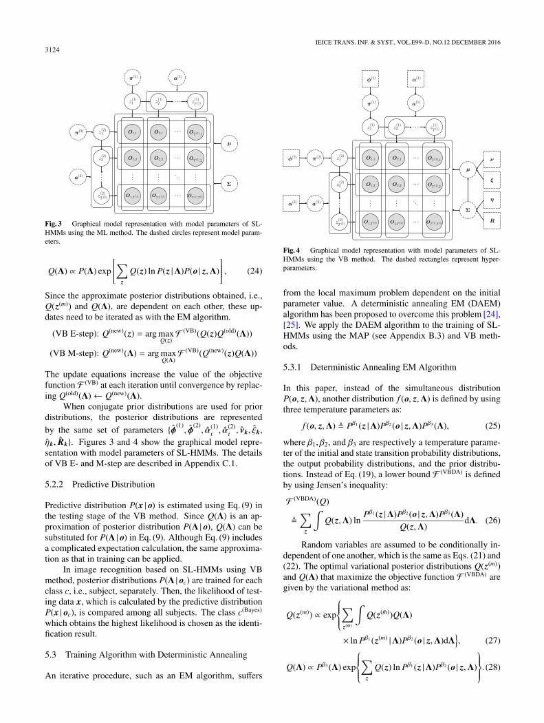
Fig. 3 Graphical model representation with model parameters of SL-HMMs using the ML method. The dashed circles represent model param-eters.
Q(Λ) ∝ P(Λ) exp
⎡⎢⎢⎢⎢⎢⎣∑
z
Q(z) ln P(z |Λ)P(o | z,Λ)
⎤⎥⎥⎥⎥⎥⎦ , (24)
Since the approximate posterior distributions obtained, i.e.,Q(z(m)) and Q(Λ), are dependent on each other, these up-dates need to be iterated as with the EM algorithm.
(VB E-step): Q(new)(z) = arg maxQ(z)F (VB)(Q(z)Q(old)(Λ))
(VB M-step): Q(new)(Λ) = arg maxQ(Λ)F (VB)(Q(new)(z)Q(Λ))
The update equations increase the value of the objectivefunction F (VB) at each iteration until convergence by replac-ing Q(old)(Λ)← Q(new)(Λ).
When conjugate prior distributions are used for priordistributions, the posterior distributions are represented
by the same set of parameters {φ(1), φ
(2), α(1)
i , α(2)i , νk, ξk,
ηk, Rk}. Figures 3 and 4 show the graphical model repre-sentation with model parameters of SL-HMMs. The detailsof VB E- and M-step are described in Appendix C.1.
5.2.2 Predictive Distribution
Predictive distribution P(x | o) is estimated using Eq. (9) inthe testing stage of the VB method. Since Q(Λ) is an ap-proximation of posterior distribution P(Λ | o), Q(Λ) can besubstituted for P(Λ | o) in Eq. (9). Although Eq. (9) includesa complicated expectation calculation, the same approxima-tion as that in training can be applied.
In image recognition based on SL-HMMs using VBmethod, posterior distributions P(Λ | oc) are trained for eachclass c, i.e., subject, separately. Then, the likelihood of test-ing data x, which is calculated by the predictive distributionP(x | oc), is compared among all subjects. The class c(Bayes)
which obtains the highest likelihood is chosen as the identi-fication result.
5.3 Training Algorithm with Deterministic Annealing
An iterative procedure, such as an EM algorithm, suffers
Fig. 4 Graphical model representation with model parameters of SL-HMMs using the VB method. The dashed rectangles represent hyper-parameters.
from the local maximum problem dependent on the initialparameter value. A deterministic annealing EM (DAEM)algorithm has been proposed to overcome this problem [24],[25]. We apply the DAEM algorithm to the training of SL-HMMs using the MAP (see Appendix B.3) and VB meth-ods.
5.3.1 Deterministic Annealing EM Algorithm
In this paper, instead of the simultaneous distributionP(o, z,Λ), another distribution f (o, z,Λ) is defined by usingthree temperature parameters as:
f (o, z,Λ) � Pβ1 (z |Λ)Pβ2 (o | z,Λ)Pβ3 (Λ), (25)
where β1, β2, and β3 are respectively a temperature parame-ter of the initial and state transition probability distributions,the output probability distributions, and the prior distribu-tions. Instead of Eq. (19), a lower bound F (VBDA) is definedby using Jensen’s inequality:
F (VBDA)(Q)
�∑
z
∫Q(z,Λ) ln
Pβ1 (z |Λ)Pβ2 (o | z,Λ)Pβ3 (Λ)Q(z,Λ)
dΛ. (26)
Random variables are assumed to be conditionally in-dependent of one another, which is the same as Eqs. (21) and(22). The optimal variational posterior distributions Q(z(m))and Q(Λ) that maximize the objective function F (VBDA) aregiven by the variational method as:
Q(z(m)) ∝ exp
⎧⎪⎪⎪⎨⎪⎪⎪⎩∑z(m)
∫Q(z(m))Q(Λ)
× ln Pβ1 (z(m) |Λ)Pβ2 (o | z,Λ)dΛ}, (27)
Q(Λ) ∝ Pβ3 (Λ) exp
⎧⎪⎪⎪⎨⎪⎪⎪⎩∑
z
Q(z) ln Pβ1 (z |Λ)Pβ2 (o | z,Λ)
⎫⎪⎪⎪⎬⎪⎪⎪⎭. (28)
SAWADA et al.: A BAYESIAN APPROACH TO IMAGE RECOGNITION BASED ON SEPARABLE LATTICE HIDDEN MARKOV MODELS3125
Fig. 5 Examples of images for the experiments.
By applying the deterministic annealing, the temperatureparameters βl are attached to the original variational pos-terior distributions, where l = 1, 2, 3 denotes the temper-ature parameter index. In the deterministic annealing pro-cess, the temperature parameters βl are gradually increasedfrom βl 0 to βl = 1. When βl 0, the variational pos-terior distributions take a form with nearly uniform distri-bution. While the temperature parameter is increasing, theform of variational posterior distributions becomes close tothat of the original variational posterior distributions. Fi-nally at βl = 1, the variational posterior distributions takethe form of the original variational posterior distributions,and the reliable model parameters can be estimated withoutthe effect of the local maximum problem. The re-estimationparameters are derived in Appendix C.2.
6. Experiments
6.1 Conditions
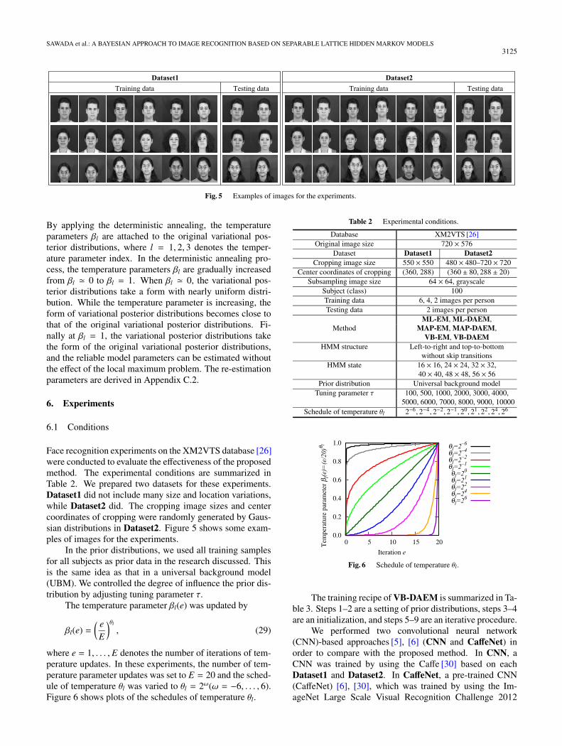
Face recognition experiments on the XM2VTS database [26]were conducted to evaluate the effectiveness of the proposedmethod. The experimental conditions are summarized inTable 2. We prepared two datasets for these experiments.Dataset1 did not include many size and location variations,while Dataset2 did. The cropping image sizes and centercoordinates of cropping were randomly generated by Gaus-sian distributions in Dataset2. Figure 5 shows some exam-ples of images for the experiments.
In the prior distributions, we used all training samplesfor all subjects as prior data in the research discussed. Thisis the same idea as that in a universal background model(UBM). We controlled the degree of influence the prior dis-tribution by adjusting tuning parameter τ.
The temperature parameter βl(e) was updated by
βl(e) =( e
E
)θl, (29)
where e = 1, . . . , E denotes the number of iterations of tem-perature updates. In these experiments, the number of tem-perature parameter updates was set to E = 20 and the sched-ule of temperature θl was varied to θl = 2ω(ω = −6, . . . , 6).Figure 6 shows plots of the schedules of temperature θl.
Table 2 Experimental conditions.
Database XM2VTS [26]Original image size 720 × 576
Dataset Dataset1 Dataset2Cropping image size 550 × 550 480 × 480–720 × 720
Center coordinates of cropping (360, 288) (360 ± 80, 288 ± 20)Subsampling image size 64 × 64, grayscale
Subject (class) 100Training data 6, 4, 2 images per personTesting data 2 images per person
ML-EM, ML-DAEM,Method MAP-EM, MAP-DAEM,
VB-EM, VB-DAEMHMM structure Left-to-right and top-to-bottom
without skip transitionsHMM state 16 × 16, 24 × 24, 32 × 32,
40 × 40, 48 × 48, 56 × 56Prior distribution Universal background model
Tuning parameter τ 100, 500, 1000, 2000, 3000, 4000,5000, 6000, 7000, 8000, 9000, 10000
Schedule of temperature θl 2−6, 2−4, 2−2, 2−1, 20, 21, 22, 24, 26
Fig. 6 Schedule of temperature θl.
The training recipe of VB-DAEM is summarized in Ta-ble 3. Steps 1–2 are a setting of prior distributions, steps 3–4are an initialization, and steps 5–9 are an iterative procedure.
We performed two convolutional neural network(CNN)-based approaches [5], [6] (CNN and CaffeNet) inorder to compare with the proposed method. In CNN, aCNN was trained by using the Caffe [30] based on eachDataset1 and Dataset2. In CaffeNet, a pre-trained CNN(CaffeNet) [6], [30], which was trained by using the Im-ageNet Large Scale Visual Recognition Challenge 2012
3126IEICE TRANS. INF. & SYST., VOL.E99–D, NO.12 DECEMBER 2016
Table 3 Training recipe of VB-DAEM.
1. Train UBM from all training samples for all subjects with flathyper-parameters.
2. Set hyper-parameters Eqs. (A· 18)–(A· 23) from UBM by adjustingtuning parameter τ.
3. Set Eqs. (A· 2)–(A· 3) to flat probabilities.4. Compute Eqs. (A· 33)–(A· 38).5. Update temperature parameters βl(e) Eq. (29).6. (VB E-step): Update Eqs. (A· 29)–(A· 31) and Eqs. (A· 2)–(A· 3).7. (VB M-step): Update Eqs. (A· 39)–(A· 44).8. Go to step 6 until convergence of lower bound F (VBDA) Eq. (26).9. Go to step 5 by adding 1 to e until e = E.
(ILSVRC2012) dataset [31], was used to extract image fea-tures. The details of CNN approaches are as follows:
CNN: The architecture of the CNN was I(64, 1) −C(128, 10, 1, 55) − P(3, 2, 27) − C(256, 5, 1, 23) −P(3, 2, 11)−F(800)−F(600)−F(400)−O(100), whereI(i, d) indicates a input layer with d dimensional i × isize image, C( f , w, s, o) indicates a convolutional layerwith f filters of w×w size window with a stride of s ando × o size output, P(w, s, o) indicates a pooling layer,F(n) indicates a fully-connected layer with n units, andO(c) indicate a output layer with c classes. The ReLUfunction and dropout with probability 0.5 were used inthe convolutional and fully-connected layers.
CaffeNet: The image-feature vectors were composed of4096 dimensions extracting the pre-trained CaffeNet ofthe 7th fully-connected layer. The one-nearest neighborwas then used as the classifier.
6.2 Results
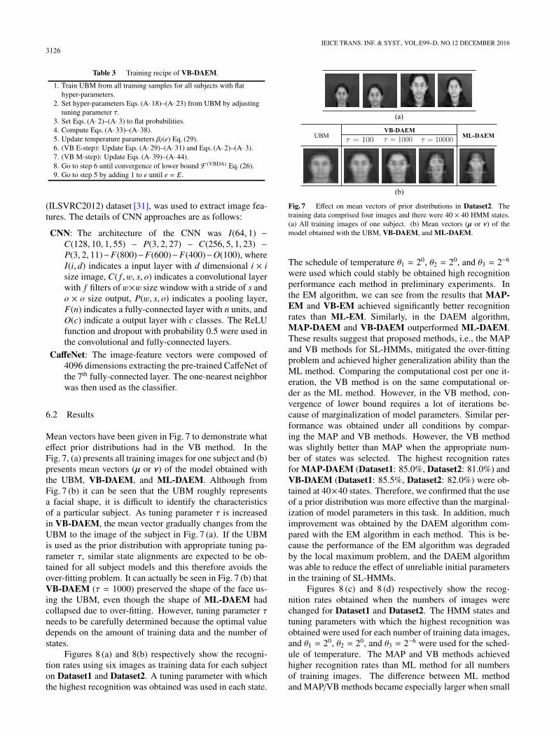
Mean vectors have been given in Fig. 7 to demonstrate whateffect prior distributions had in the VB method. In theFig. 7, (a) presents all training images for one subject and (b)presents mean vectors (μ or ν) of the model obtained withthe UBM, VB-DAEM, and ML-DAEM. Although fromFig. 7 (b) it can be seen that the UBM roughly representsa facial shape, it is difficult to identify the characteristicsof a particular subject. As tuning parameter τ is increasedin VB-DAEM, the mean vector gradually changes from theUBM to the image of the subject in Fig. 7 (a). If the UBMis used as the prior distribution with appropriate tuning pa-rameter τ, similar state alignments are expected to be ob-tained for all subject models and this therefore avoids theover-fitting problem. It can actually be seen in Fig. 7 (b) thatVB-DAEM (τ = 1000) preserved the shape of the face us-ing the UBM, even though the shape of ML-DAEM hadcollapsed due to over-fitting. However, tuning parameter τneeds to be carefully determined because the optimal valuedepends on the amount of training data and the number ofstates.
Figures 8 (a) and 8(b) respectively show the recogni-tion rates using six images as training data for each subjecton Dataset1 and Dataset2. A tuning parameter with whichthe highest recognition was obtained was used in each state.
Fig. 7 Effect on mean vectors of prior distributions in Dataset2. Thetraining data comprised four images and there were 40 × 40 HMM states.(a) All training images of one subject. (b) Mean vectors (μ or ν) of themodel obtained with the UBM, VB-DAEM, and ML-DAEM.
The schedule of temperature θ1 = 20, θ2 = 20, and θ3 = 2−6
were used which could stably be obtained high recognitionperformance each method in preliminary experiments. Inthe EM algorithm, we can see from the results that MAP-EM and VB-EM achieved significantly better recognitionrates than ML-EM. Similarly, in the DAEM algorithm,MAP-DAEM and VB-DAEM outperformed ML-DAEM.These results suggest that proposed methods, i.e., the MAPand VB methods for SL-HMMs, mitigated the over-fittingproblem and achieved higher generalization ability than theML method. Comparing the computational cost per one it-eration, the VB method is on the same computational or-der as the ML method. However, in the VB method, con-vergence of lower bound requires a lot of iterations be-cause of marginalization of model parameters. Similar per-formance was obtained under all conditions by compar-ing the MAP and VB methods. However, the VB methodwas slightly better than MAP when the appropriate num-ber of states was selected. The highest recognition ratesfor MAP-DAEM (Dataset1: 85.0%, Dataset2: 81.0%) andVB-DAEM (Dataset1: 85.5%, Dataset2: 82.0%) were ob-tained at 40×40 states. Therefore, we confirmed that the useof a prior distribution was more effective than the marginal-ization of model parameters in this task. In addition, muchimprovement was obtained by the DAEM algorithm com-pared with the EM algorithm in each method. This is be-cause the performance of the EM algorithm was degradedby the local maximum problem, and the DAEM algorithmwas able to reduce the effect of unreliable initial parametersin the training of SL-HMMs.
Figures 8 (c) and 8 (d) respectively show the recog-nition rates obtained when the numbers of images werechanged for Dataset1 and Dataset2. The HMM states andtuning parameters with which the highest recognition wasobtained were used for each number of training data images,and θ1 = 20, θ2 = 20, and θ3 = 2−6 were used for the sched-ule of temperature. The MAP and VB methods achievedhigher recognition rates than ML method for all numbersof training images. The difference between ML methodand MAP/VB methods became especially larger when small

SAWADA et al.: A BAYESIAN APPROACH TO IMAGE RECOGNITION BASED ON SEPARABLE LATTICE HIDDEN MARKOV MODELS3127
Fig. 8 Recognition rates obtained in image recognition experiments. (a) The effect of the number ofHMM states on Dataset1. (b) The effect of the number of HMM states on Dataset2. (c) The effect ofthe amount of training data on Dataset1. (d) The effect of the amount of training data on Dataset2.
Table 4 Recognition rates obtained in schedule of temperature experiments. Where θ1, θ2, and θ3 arerespectively a schedule of the initial and state transition probability distributions, the output probabilitydistributions, and the prior distributions. Bold numbers indicate recognition rates of 87.0% or more.
θ1 20 21 22 24 26 20 21 22 24 26 20 21 22 24 26
θ2 20 21 22
2−6 85.5 85.0 85.0 85.5 85.5 85.0 84.5 85.5 86.0 86.5 84.5 85.5 85.5 87.0 86.52−4 84.0 83.5 83.5 83.5 83.5 85.5 85.0 84.5 86.5 86.5 85.0 85.5 84.5 86.0 86.0
θ3 2−2 85.5 84.5 85.0 85.0 85.0 86.0 86.0 86.0 86.0 86.0 85.5 86.0 85.0 85.5 85.52−1 80.0 80.5 81.0 80.0 80.5 85.5 87.0 87.5 88.0 88.0 85.0 86.0 87.0 87.0 87.020 77.5 78.0 78.0 77.5 78.0 85.0 85.0 84.5 84.5 84.5 85.5 86.0 86.0 86.5 86.5
numbers of training images were used. These results clearlyshow that the proposed methods can estimate high general-ization ability when there is insufficient training data. Bycontrast, it is considered that the difference ML method andMAP/VB methods become smaller when there is sufficienttraining data. Although the MAP and the VB methods hadalmost the same recognition rates, VB-DAEM (Dataset1:54.0%, Dataset2: 52.0%) obtained better recognition ratesthan MAP-DAEM (Dataset1: 51.0%, Dataset2: 50.0%)when only two training images were used. Comparing theproposed method with CNN, VB-DAEM achieved betterrecognition rates than CNN. These results indicate that theproposed method is more effective than CNN when theamount of training data is insufficient. However, the numberof training images in the experiments was small to train theCNN. Therefore, in the future, we should perform on largedatasets. Although VB-DAEM and CaffeNet had almostthe same recognition rates in Dataset1, VB-DAEM outper-formed CaffeNet in Dataset2. These results suggest thatthe proposed method is more robust to geometric variationsthan CaffeNet.
The effect of the schedule of temperature θl was eval-uated in VB-DAEM. Table 4 shows recognition rates ob-tained in the experiments. Six images in Dataset1 were used
as training data for each subject. SL-HMMs with 40 × 40states and tuning parameter τ = 4000 were used in the ex-periments. Recognition rates was improved by using theappropriate schedule of temperature θl. By contrast, an in-appropriate schedule caused a decrease in the performanceof generalization ability. Statistics of UBM used in priordistributions are high reliability because it is trained in ad-vance. On the other hand, statistics of training data are lowreliability in early stage of training. Therefore, high recog-nition rates was obtained by bringing the schedule of tem-perature θl = 1 in the order of θ3, θ2, and θ1. As future work,a method of automatically determining the schedule will beneeded to obtain an appropriate schedule.
7. Conclusion
This paper proposed an image recognition method based onseparable lattice hidden Markov models (SL-HMMs) usingthe maximum a posteriori (MAP) and variational Bayesian(VB) methods. An improved training algorithm using thedeterministic annealing expectation maximization (DAEM)algorithm was also derived. Face recognition experimentsperformed on the XM2VTS database showed that the MAPand VB methods offer better recognition performance than

3128IEICE TRANS. INF. & SYST., VOL.E99–D, NO.12 DECEMBER 2016
the maximum likelihood (ML) method. These results sug-gest that the MAP and VB methods are useful for imagerecognition applications based on SL-HMMs. The use ofprior distributions was more effective than the marginaliza-tion of model parameters in this task. The DAEM algorithmwas able to reduce the effect of unreliable initial parame-ters in the training of SL-HMMs. Additionally, compar-ative experiment results showed that the proposed methodwas more robust to geometric variations than convolutionalneural networks. Subjects for future work include applyingthe Bayesian criterion to image recognition based on hid-den Markov eigen-image models [20], which integrate SL-HMMs and factor analyzers, and performing experimentson various image recognition tasks.
Acknowledgments
This work was supported by Grant-in-aid for JSPS FellowsGrant Number 15J08391 and the Hori Sciences and ArtsFoundation.
References
[1] M.A. Turk and A.P. Pentland, “Face recognition using eigen-faces,” Conference on Computer Vision and Pattern Recognition,pp.586–591, 1991.
[2] S. Watanabe and N. Pakvasa, “Subspace method of pattern recogni-tion,” International Joint Conference on Pattern Recognition, pp.25–32, 1973.
[3] D.G. Lowe, “Distinctive image features from scale-invariant key-points,” Int. J. Comput. Vision., vol.60, no.2, pp.91–110, 2004.
[4] N. Dalal and B. Triggs, “Histograms of oriented gradients for humandetection,” Conference on Computer Vision and Pattern Recogni-tion, pp.886–893, 2005.
[5] Y. Lecun, L. Bottou, Y. Bengio, and P. Haffner, “Gradient-basedlearning applied to document recognition,” Proc. IEEE, vol.86,no.11, pp.2278–2324, 1998.
[6] A. Krizhevsky, I. Sutskever, and G.E. Hinton, “ImageNet classifica-tion with deep convolutional neural networks,” Conference on Neu-ral Information Processing Systems, pp.1097–1105, 2012.
[7] F.S. Samaria, Face recognition using hidden Markov models, Ph. D.dissertation, University of Cambridge, 1994.
[8] A.V. Nefian and M.H. Hayes, “Hidden Markov models for facerecognition,” International Conference on Acoustics, Speech andSignal Processing, vol.5, pp.2721–2724, 1998.
[9] S.-S. Kuo and O.E. Agazzi, “Keyword spotting in poorly printeddocuments using pseudo 2-D hidden Markov models,” IEEE Trans.Pattern Anal. Machine Intell., vol.16, no.8, pp.842–848, 1994.
[10] A.V. Nefian and M.H. Hayes, “Maximum likelihood training of theembedded HMM for face detection and recognition,” InternationalConference on Image Processing, vol.1, pp.33–36, 2000.
[11] X. Ma, W.A. Pearlman, J.W. Woods, D. Schonfeld, A. Khokhar,and L. Lu, “Image segmentation and classification based on a 2Ddistributed hidden Markov model,” Society of Photo-optical Instru-mentation Engineers, vol.6822, 2008.
[12] J. Li, A. Najmi, and R.M. Gra, “Image classification by a two dimen-sional hidden Markov model,” IEEE Trans. Signal Process., vol.48,no.2, pp.517–533, 2000.
[13] H. Othman and T. Aboiilnasr, “A simplified second-order HMMwith application to face recognition,” International Symposium onCircuits and Systems, vol.2, pp.161–164, 2001.
[14] J.-T. Chien and C.-P. Liao, “Maximum confidence hidden Markovmodeling for face recognition,” IEEE Trans. Pattern Anal. Mach.
Intell., vol.30, no.4, pp.606–616, 2008.[15] D. Kurata, Y. Nankaku, K. Tokuda, T. Kitamura, and Z. Ghahramani,
“Face recognition based on separable lattice HMMs,” InternationalConference on Acoustics, Speech and Signal Processing, vol.5,pp.737–740, 2006.
[16] A. Tamamori, Y. Nankaku, and K. Tokuda, “An extension of separa-ble lattice 2-D HMMs for rotational data variations,” IEICE Trans.Inf. & Syst., vol.E95-D, no.8, pp.2074–2083, 2012.
[17] K. Kumaki, Y. Nankaku, and K. Tokuda, “Face recognition based onextended separable lattice 2-D HMMs,” International Conference onAcoustics, Speech and Signal Processing, pp.2209–2212, 2012.
[18] Y. Takahashi, A. Tamamori, Y. Nankaku, and K. Tokuda, “Facerecognition based on separable lattice 2-D HMM with state dura-tion modeling,” International Conference on Acoustics, Speech andSignal Processing, pp.2162–2165, 2010.
[19] A. Tamamori, Y. Nankaku, and K. Tokuda, “Image recognitionbased on separable lattice trajectory 2-D HMMs,” IEICE Trans. Inf.& Syst., vol.E97-D, no.7, pp.1842–1854, 2014.
[20] Y. Nankaku and K. Tokuda, “Face recognition using hidden Markoveigenface models,” International Conference on Acoustics, Speechand Signal Processing, vol.2, pp.469–472, 2007.
[21] J.-L. Gauvain and C.-H. Lee, “Maximum a posteriori estimationfor multivariate Gaussian mixture observations of Markov chains,”IEEE Trans. Speech Audio Process., vol.2, no.2, pp.291–298, 1994.
[22] H. Attias, “Inferring parameters and structure of latent variable mod-els by variational Bayes,” Conference on Uncertainty in ArtificialIntelligence, pp.21–30, 1999.
[23] K. Sawada, A. Tamamori, K. Hashimoto, Y. Nankaku, and K.Tokuda, “Face recognition based on separable lattice 2-D HMMsusing variational bayesian method,” International Conference onAcoustics, Speech and Signal Processing, pp.2205–2208, 2012.
[24] N. Ueda and R. Nakano, “Deterministic annealing EM algorithm,”Neural Networks, vol.11, no.2, pp.271–282, 1998.
[25] K. Katahira, K. Watanabe, and M. Okada, “Deterministic annealingvariant of variational Bayes method,” Journal of Physics: Confer-ence Series, vol.95, 012015, 2008.
[26] K. Messer, J. Matas, J. Kittler, and K. Jonsson, “XM2VTSDB: Theextended M2VTS database,” International Conference on Audio andVideo-based Biometric Person Authentication, pp.72–77, 1999.
[27] B.P. Carlin and S. Chib, “Bayesian model choice via Markov chainMonte Carlo,” J. Royal Statistical Society, vol.57, no.3, pp.473–484,1995.
[28] A.P. Dempster, N.M. Laird, and D.B. Rubin, “Maximum likelihoodfrom incomplete data via the EM algorithm,” J. Royal Statistical So-ciety: Series B, vol.39, no.1, pp.1–38, 1977.
[29] M.I. Jordan, Z. Ghahramani, T.S. Jaakkola, and L.K. Saul, “An in-troduction to variational methods for graphical models,” MachineLearning, vol.37, no.2, pp.183–233, 1999.
[30] Y. Jia, E. Shelhamer, J. Donahue, S. Karayev, J. Long, R.B. Girshick,S. Guadarrama, and T. Darrell, “Caffe: Convolutional architecturefor fast feature embedding,” ACM international conference on Mul-timedia, pp.675–678, 2014.
[31] O. Russakovsky, J. Deng, H. Su, J. Krause, S. Satheesh, S. Ma, Z.Huang, A. Karpathy, A. Khosla, M. Bernstein, A.C. Berg, and L.Fei-Fei, “ImageNet Large Scale Visual Recognition Challenge,” Int.J. Comput. Vision., vol.115, no.3, pp.211–252, 2015.
[32] L.R. Rabiner and B.H. Juang, “An introduction to hidden Markovmodels,” IEEE ASSP Magazine, vol.3, no.1, pp.4–16, 1986.
Appendix A: Derivation of ML Method for SL-HMMs
A.1 EM Algorithm for ML Method
The variational posterior distribution Q(z(m)) can be repre-sented as follows:

SAWADA et al.: A BAYESIAN APPROACH TO IMAGE RECOGNITION BASED ON SEPARABLE LATTICE HIDDEN MARKOV MODELS3129
Q(z(m))∝ exp
⎡⎢⎢⎢⎢⎢⎢⎣K(m)∑i=1
z(m)i,1 ln π(m)
i
⎤⎥⎥⎥⎥⎥⎥⎦
× exp
⎡⎢⎢⎢⎢⎢⎢⎣T (m)∑
t(m)=2
K(m)∑i=1
K(m)∑j=1
z(m)i,t(m)−1
z(m)j,t(m) ln a(m)
i j
⎤⎥⎥⎥⎥⎥⎥⎦
× exp
⎡⎢⎢⎢⎢⎢⎢⎣∑
t
K(m)∑i=1
K(m)∑j=1
z(m)i,t(m)〈z(m)
j,t(m)〉Q(z(m)) ln bk(ot)
⎤⎥⎥⎥⎥⎥⎥⎦ . (A· 1)
The expectation value with respect to Q(z(m)) is computedin the E-step by the following equations:
〈z(m)i,t(m)〉Q(z(m)) =
∑z(m)
Q(z(m))z(m)i,t(m) , (A· 2)
〈z(m)i,t(m)−1
z(m)j,t(m)〉Q(z(m)) =
∑z(m)
Q(z(m))z(m)i,t(m)−1
z(m)j,t(m) , (A· 3)
〈zk,t〉Q(z) =∑z(1)
∑z(2)
Q(z(1))Q(z(2))z(1)i,t(1) z
(2)j,t(2) , (A· 4)
where 〈·〉Q(·) denotes the expectation with respect to the pos-terior distribution Q(·) and z(m)
i,t(m) is the Kronecker delta func-tion:
z(m)i,t(m) = δ(z
(m)t(m) , i) =
⎧⎪⎨⎪⎩ 0 (z(m)t(m) � i)
1 (z(m)t(m) = i)
. (A· 5)
The variational posterior distribution Q(z(m)) in Eq. (A· 1)has a Markovian structure as the likelihood function of anstandard one-dimensional HMM. Therefore, Eqs. (A· 2) and(A· 3) can be computed efficiently by the forward-backwardalgorithm given in [32].
In the M-step, the model parameters of the SL-HMMscan be updated by sufficient statistics of the training data asfollows:
π(m)i = 〈z(m)
i,1 〉Q(z(m)), (A· 6)
a(m)i j =
N(m)i j∑T (m)
t(m)=2〈z(m)i−1,t(m)〉Q(z(m))
, (A· 7)
μk = Fk, (A· 8)
Σk =Sk, (A· 9)
where statistics N(m)i j , Fk, and Sk are represented as follows:
N(m)i j =
T (m)∑t(m)=2
〈z(m)i,t(m)−1
z(m)j,t(m)〉Q(z(m)), (A· 10)
Nk =∑
t
〈zk,t〉Q(z), (A· 11)
Fk =1
Nk
∑t
〈zk,t〉Q(z)ot , (A· 12)
Sk =1
Nk
∑t
〈zk,t〉Q(z)(ot − Fk)(ot − Fk)�. (A· 13)
Appendix B: Derivation of MAP Method for SL-HMMs
B.1 EM Algorithm for MAP Method
The model parameters of SL-HMMs using the MAP methodcan be updated by sufficient statistics and hyper-parametersas follows:
π(m)i =
〈z(m)i,1 〉Q(z(m)) + φ
(m)i − 1
1 +∑K(m)
i′=1 (φ(m)i′ − 1)
, (A· 14)
a(m)i j =
N(m)i j + α
(m)i j − 1∑T (m)
t(m)=2〈z(m)i−1,t(m)〉Q(z(m)) +
∑K(m)
j′=1(α(m)i j′ − 1)
, (A· 15)
μk =NkFk + ξkνk
Nk + ξk, (A· 16)
Σk =1
Nk + ηk − D
⎡⎢⎢⎢⎢⎢⎣∑
t
〈zk,t〉Q(z)(ot − μk)(ot − μk)�
+ξk(μk − νk)(μk − νk)� + Rk
], (A· 17)
where D is a dimension of observation o.
B.2 Hyper-Parameters
The hyper-parameters based on prior data are given as:
φ(m)i =
〈z(m)i,t(m)〉Q(z(m))
τ+ 1, (A· 18)
α(m)i j =
N(m)i j
τ+ 1, (A· 19)
νk = Fk, (A· 20)
ξk =Nk
τ, (A· 21)
ηk =Nk
τ+ D, (A· 22)
Rk =Nk
τSk, (A· 23)
where · denotes statistics of prior data and τ is the tuningparameter.
B.3 DAEM Algorithm for MAP Method
The model parameters of SL-HMMs using the MAP methodwith the DAEM algorithm can be updated by sufficientstatistics and hyper-parameters as follows:
π(m)i =
β1〈z(m)i,1 〉Q(z(m)) + β3(φ(m)
i − 1)
β1 + β3∑K(m)
i′=1 (φ(m)i′ − 1)
, (A· 24)
a(m)i j =
β1N(m)i j + β3(α(m)
i j − 1)
β1∑T (m)
t(m)=2〈z(m)i−1,t(m)〉Q(z(m)) + β3
∑K(m)
j′=1(α(m)i j′ − 1)
, (A· 25)
μk =β2NkFk + β3ξkνk
β2Nk + β3ξk, (A· 26)

3130IEICE TRANS. INF. & SYST., VOL.E99–D, NO.12 DECEMBER 2016
Σk =1
β2Nk + β3(ηk − D)
×⎡⎢⎢⎢⎢⎢⎣β2
∑t
〈zk,t〉Q(z)(ot − μk)(ot − μk)�
+β3ξk(μk − νk)(μk − νk)� + β3Rk
]. (A· 27)
Appendix C: Derivation of VB Method for SL-HMMs
C.1 EM Algorithm for VB Method
In the VB E-step, the optimal variational posterior distribu-tions Q(z(m)) that maximize the objective function F (VB) aregiven as:
Q(z(m))∝ exp
⎡⎢⎢⎢⎢⎢⎢⎣K(m)∑i=1
z(m)i,1 〈ln π(m)
i 〉Q(π(m))
⎤⎥⎥⎥⎥⎥⎥⎦
× exp
⎡⎢⎢⎢⎢⎢⎢⎣T (m)∑
t(m)=2
K(m)∑i=1
K(m)∑j=1
z(m)i,t(m)−1
z(m)j,t(m)〈ln a(m)
i j 〉Q(a(m)i )
⎤⎥⎥⎥⎥⎥⎥⎦
× exp
⎡⎢⎢⎢⎢⎢⎢⎣∑
t
K(m)∑i=1
K(m)∑j=1
z(m)i,t(m)〈z(m)
j,t(m)〉Q(z(m))〈ln bk(ot)〉Q(bk)
⎤⎥⎥⎥⎥⎥⎥⎦ , (A· 28)
The updates of the expectations of model parameters are de-rived as:
〈ln π(m)i 〉Q(π(m)) =Ψ (φ(m)
i ) − Ψ⎛⎜⎜⎜⎜⎜⎜⎝
K(m)∑i′=1
φ(m)i′
⎞⎟⎟⎟⎟⎟⎟⎠ , (A· 29)
〈ln a(m)i j 〉Q(a(m)
i ) =Ψ (α(m)i j ) − Ψ
⎛⎜⎜⎜⎜⎜⎜⎝K(m)∑j′=1
α(m)i j′
⎞⎟⎟⎟⎟⎟⎟⎠ , (A· 30)
〈ln bk(ot)〉Q(bk) =−12
⎧⎪⎪⎨⎪⎪⎩D ln π +D
ξk−
D∑d=1
Ψ
(ηk + 1 − d
2
)
+ ln |Rk| + Tr[ηkR
−1k (ot − νk)(ot − νk)�
]}, (A· 31)
where Ψ (·) is a digamma function. The expectation valuein Eqs. (A· 2) and (A· 3) can be computed efficiently by theforward-backward algorithm given in [32].
In the VB M-step, the optimal variational posterior dis-tributions Q(Λ) that maximize the objective function F (VB)
are given as:
Q(Λ)∝ P(Λ)2∏
m=1
⎧⎪⎪⎨⎪⎪⎩exp
⎡⎢⎢⎢⎢⎢⎢⎣K(m)∑i=1
〈z(m)i,t(m)〉Q(z(m)) ln π(m)
i
⎤⎥⎥⎥⎥⎥⎥⎦
× exp
⎡⎢⎢⎢⎢⎢⎢⎣T (m)∑
t(m)=2
K(m)∑i=1
K(m)∑j=1
〈z(m)i,t(m)−1
z(m)j,t(m)〉Q(z(m)) ln a(m)
i j
⎤⎥⎥⎥⎥⎥⎥⎦⎫⎪⎪⎬⎪⎪⎭
× exp
⎡⎢⎢⎢⎢⎢⎣∑
t
∑k
〈zk,t〉Q(z) ln bk(ot)
⎤⎥⎥⎥⎥⎥⎦ , (A· 32)
The posterior distribution of model parameters Q(Λ) can beupdated by statistics of the training data as follows:
φ(m)i = 〈z(m)
i,1 〉Q(z(m)) + φ(m)i , (A· 33)
α(m)i j =N(m)
i j + α(m)i j , (A· 34)
νk =NkFk + ξkνk
Nk + ξk, (A· 35)
ξk =Nk + ξk, (A· 36)
ηk =Nk + ηk, (A· 37)
Rk =NkSk +Nkξk
Nk + ξk(Fk − νk)(Fk − νk)� + Rk. (A· 38)
C.2 DAEM Algorithm for VB Method
In the VB E-step, the forward-backward algorithm is ap-plied by taking temperature parameters into account. In theVB M-step, the posterior distribution of model parametersQ(Λ) can be updated by statistics of the training data as fol-lows:
φ(m)i = β1〈z(m)
i,1 〉Q(z(m)) + β3(φ(m)i − 1) + 1, (A· 39)
α(m)i j = β1N(m)
i j + β3(α(m)i j − 1) + 1, (A· 40)
νk =β2NkFk + β3ξkνk
β2Nk + β3ξk, (A· 41)
ξk = β2Nk + β3ξk, (A· 42)
ηk = β2Nk + β3(ηk − D) + D, (A· 43)
Rk = β2NkSk +β2β3Nkξk
β2Nk + β3ξk(Fk − νk)(Fk − νk)� + β3Rk.
(A· 44)
Kei Sawada received the B.E. and M.E.degrees in Computer Science and Scientific andEngineering Simulation from Nagoya Instituteof Technology, Nagoya, Japan, in 2011 and2013. He is currently a Ph.D. candidate at Na-goya Institute of Technology. From June 2014 toNovember 2014, he was a visiting researcher atthe University of Edinburgh. Since April 2015,he has been a Research Fellow of the Japan So-ciety for the Promotion of Science (DC2) at Na-goya Institute of Technology, Nagoya, Japan.
His research interests include image recognition, speech recognition andsynthesis, and machine learning. He is a student member of the Insti-tute of Electronics, Information and Communication Engineers (IEICE),the Acoustical Society of Japan (ASJ) and International Speech Communi-cation Association (ISCA).
SAWADA et al.: A BAYESIAN APPROACH TO IMAGE RECOGNITION BASED ON SEPARABLE LATTICE HIDDEN MARKOV MODELS3131
Akira Tamamori received the B.E. de-gree in Computer Science, the M.E. and Ph.D.degrees in the Department of Scientific andEngineering Simulation from Nagoya Instituteof Technology, Nagoya, Japan, in 2008, 2010,2014, respectively. He is now a Visiting Assis-tant Professor at the same institute. His researchinterests include statistical machine learning,image recognition, and speech signal process-ing. He is a member of the Institute of Electron-ics, Information and Communication Engineers
(IEICE) and the Acoustical Society of Japan (ASJ).
Kei Hashimoto received the B.E., M.E.,and Ph.D. degrees in computer science, com-puter science and engineering, and scientific andengineering simulation from Nagoya Institute ofTechnology, Nagoya, Japan in 2006, 2008, and2011, respectively. From October 2008 to Jan-uary 2009, he was an intern researcher at Na-tional Institute of Information and Communica-tions Technology (NICT), Kyoto, Japan. FromApril 2010 to March 2012, he was a ResearchFellow of the Japan Society for the Promotion
of Science (JSPS) at Nagoya Institute of Technology, Nagoya, Japan. FromMay 2010 to September 2010, he was a visiting researcher at Universityof Edinburgh and Cambridge University. From April 2012, he is now anAssistant Professor at Nagoya Institute of Technology, Nagoya, Japan. Hisresearch interests include statistical speech synthesis and speech recogni-tion. He is a member of the Acoustical Society of Japan.
Yoshihiko Nankaku received his B.E. de-gree in Computer Science, and his M.E. andPh.D. degrees in the Department of Electricaland Electronic Engineering from Nagoya Insti-tute of Technology, Nagoya, Japan, in 1999,2001, and 2004 respectively. After a year as apostdoctoral fellow at the Nagoya Institute ofTechnology, he became an Associate Professorat the same Institute. He was a visiting re-searcher at the Department of Engineering, Uni-versity of Cambridge, UK, from May to October
2011. His research interests include statistical machine learning, speechrecognition, speech synthesis, image recognition, and multi-modal inter-face. He is a member of the Institute of Electronics, Information and Com-munication Engineers (IEICE) and the Acoustical Society of Japan (ASJ).
Keiichi Tokuda received the B.E. degree inelectrical and electronic engineering from Na-goya Institute of Technology, Nagoya, Japan,the M.E. and Dr.Eng. degrees in informationprocessing from the Tokyo Institute of Technol-ogy, Tokyo, Japan, in 1984, 1986, and 1989,respectively. From 1989 to 1996 he was a Re-search Associate at the Department of Elec-tronic and Electric Engineering, Tokyo Instituteof Technology. From 1996 to 2004 he was aAssociate Professor at the Department of Com-
puter Science, Nagoya Institute of Technology as Associate Professor, andnow he is a Professor at the same institute. He is also an Honorary Profes-sor at the University of Edinburgh. He was an Invited Researcher at ATRSpoken Language Translation Research Laboratories, Japan from 2000 to2013 and was a Visiting Researcher at Carnegie Mellon University from2001 to 2002. He published over 80 journal papers and over 190 confer-ence papers, and received six paper awards and three achievement awards.He was a member of the Speech Technical Committee of the IEEE Sig-nal Processing Society from 2000 to 2003, a member of ISCA AdvisoryCouncil and an associate editor of IEEE Transactions on Audio, Speech& Language Processing, and acts as organizer and reviewer for many ma-jor speech conferences, workshops and journals. He is a IEEE Fellow andISCA Fellow. His research interests include speech coding, speech synthe-sis and recognition, and statistical machine learning.