A Method for Modeling Clouds based on Atmospheric Fluid Dynamics

Ryo Miyazaki Satoru Yoshida Yoshinori Dobashi† Tomoyuki Nishita University of Tokyo †Hokkaido University

7-3-1, Hongo, Bunkyo-ku Kita 13, Nishi 8, Kita-ku, Tokyo, 113-0033, Japan Sapporo, 060-8628, Japan

{ryomiya, yoshida, nis}@nis-lab.is.s.u-tokyo.ac.jp doba@nis-ei.eng.hokudai.ac.jp

Abstract

The simulation of natural phenomena such as clouds, smoke, fire and water is one of the most important research areas in computer graphics. In particular, clouds play an important role in creating images of outdoor scenes. The proposed method is based on the physical simulation of atmospheric fluid dynamics which characterizes the shape of clouds. To take account of the dynamics, we used a method called the coupled map lattice (CML). CML is an extended method of cellular automaton and is computationally inexpensive. The proposed method can create various types of clouds and can also realize the animation of these clouds. Moreover, we have developed an interactive system for modeling various types of clouds. Keywords : Clouds, natural phenomena, simulation, Coupled Map Lattice, cellular automaton, metaballs. 1. Introduction

Clouds play an important role when generating such images as outdoor scenes, the earth viewed from outer space and the visualization of weather information. The cloud shape depends on the environment under which they are formed, such as ascending air currents, temperature and humidity. We often observe fascinating cloud shapes. For example, cumulonimbi over the sea on a hot day in summer and cirrocumuli at sunset in the fall are extremely imp ressive. Therefore, many researchers have been trying to create realistic images of clouds.

Clouds are classified into ten types , based on their shape and altitude [1]. However, using previous methods it was difficult to create the various kinds of clouds by using a single algorithm. To address this problem, this paper proposes a new method for modeling various types of clouds. The basic idea of the proposed method is to create clouds by simulating the physical process, especially atmospheric fluid dynamics which characterize the shape of clouds. There has been little research based

on physical simulation, since the exact simulation of atmospheric fluid dynamics is very difficult and computationally expensive. However, exact simulation is not important in order to model visually convincing clouds.

Our method simulates cloud formation using a simplified numerical model, called the coupled map lattice (CML) . CML was originally developed by Kaneko [2] and is an extended method of cellular automaton. The advantages of using the coupled map lattice are that it is easy to implement and the computational cost is small. Yanagita et al. proposed a method for the modeling and characterization of cloud dynamics using the coupled map lattice [3]. Unfortunately, their method is not sufficient for our purpose, since their aim was not to create realistic images of clouds. Furthermore, in their paper, cloud formation is simulated in two -dimensional space only. Therefore, we extend their work and propose a new method to create realistic images. Furthermore, we propose an interactive system for cloud modeling. In this system, the clouds created by our method are obtained as a three-dimensional density distribution. Therefore, realistic images can be generated by simulating various optical phenomena such as light scattering and absorption due to cloud particles. The animation of clouds can also be realized, since our method actually simulates the cloud evolution. 2. Previous Work

Many methods for modeling the shapes and motion of clouds have been proposed in computer graphics. These can be classified into three categories.

The first of these simulates the physical process of fluid dynamics [4] [5] [6]. Most of these methods require a large amount of computation time. Stam, however, developed a fast simulation method by simplifying fluid dynamics [7]. He demonstrated the real-time animation of smoke on a high-end workstation. His method is, however, focused on the motion of smoke and the

possibility of the application of his method to modeling various types of clouds is not discussed. Moreover, the phenomenon known as phase transition is not taken into account. Phase transition is important in the cloud formation process; water vapor in the air becomes water droplets, or clouds. In computer graphics, Kajiya et al. developed a method taking into account these phase transition effects [8]. In this method, the atmospheric fluid dynamics are solved numerically. However, this is very complex and requires a great deal of computational cost. Recently, Dobashi et al. developed a fast method for simulating cloud motion using the idea of cellular automaton [9]. In their method, however, the modeling of various types of clouds seems to be difficult , since they use an extremely simplified model for the physical process of cloud formation. In fact, only cumulus clouds are demonstrated in their paper.

The second approach is the heuristic approach. The methods that take this approach use fractals [10] [11] [12] [13], procedural modeling [14] [15] [16] [17] [18] [19], qualitative simulation [20] [21] and stochastic modeling [22]. These methods are computationally inexpensive and much easier to implement. However, to employ these methods, users have to adjust many parameters by trial and error in order to create various kinds of clouds.

The third approach is a type of image-based modeling. Dobashi et al. used satellite images to create clouds such as the typhoon as it appears viewed from space [23]. However, users of this method cannot create all of the desirable shapes of clouds, because this method requires satellite images.

This paper addresses the problems of the previous methods and proposes a new method for modeling various kinds of clouds. Our method simulates the cloud formation process using CML. CML has been used for the analysis of several natural phenomena [2] [24] [25] [26] [27] [28] [29] [30]. Yanagita et al. proposed a method for simulating cloud formation using CML [3]. The purpose of their paper, however, is to clarify the qualitative characteristics of the physical phenomenon and not to create realistic images. 3. Overview of Our Method

We first need to explain about cloud shape and formation in order to give a better understanding of our method before we give an overview of the process.

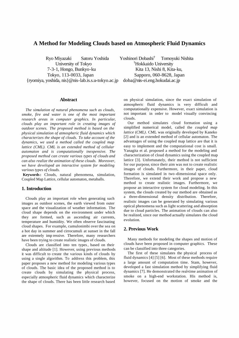
In general, clouds are classified by their appearance into 10 different types [1]. Fig. 1 shows photographs of representative clouds. Cumulus clouds are generally dense and have a sharp outline (see Fig. 1(a)). Cumulonimbus is an advanced stage of cumulus development with considerable vertical extent, in the form of a mountain or huge towers (see Fig. 1(b)). Stratus and stratocumulus are low-level clouds. Stratus is

generally a grey broadsheet with a fairly uniform sheet appearance. Stratocumulus is a layer of cloud composed of rounded masses, rolls, etc, which are clearly identifiable elements. Nimbostratus is a grey cloud layer, often dark. Altostratus and Altocumulus are mid-altitude clouds. Altostratus is a sheet or layer of clouds with a striated and uniform appearance, which totally or partially covers the sky. Altocumulus is composed of rounded masses, rolls, etc. Altocumulus is usually quite thin (Fig. 1(c)). Cirrus, cirrostratus, and cirrocumulus are high-altitude clouds, and consist almost entirely of ice particles. Cirrus consists of detached clouds in the form of white, delicate filaments or mostly white patches or narrow bands. These clouds have a hair-like appearance, or a silky sheen, or both. Cirrostratus is a transparent, whitish cloud veil of hair-like or smooth appearance, totally or partly covering the sky. Cirrocumulus is a thin white patch, sheet or layer of cloud composed of very small elements in the form of grains, ripples, etc. Cirrocumulus is the high-altitude counterpart of altocumulus, and it has species and varieties similar to those of altocumulus (see Fig. 1(d)).

(a) cumulus (b) cumulonimbus

(c) altocumulus (d) cirrocumulus

Figure 1. Photographs of clouds.

Alternatively, clouds can be classified into roughly two different types based on the way that they are formed. Clouds in the first type are known as cumuliform (cumulus and cumulonimbus), and they are formed by strong ascending air currents. The essential difference of formation process between cumuli and cumulonimbi is the strength of the ascending air currents. Clouds in the second category are generated by the cooling down of vapor that flows upward from the ground. In particular, the patterns observed in the cell-like or roll-like shapes of stratocumulus, altocumulus, and cirrocumulus are generated by the Bénard convection. The differences between them are their relative height and scale. Cirrocumulus is generated in higher altitudes and the size

of the Bénard cell (see Section 4.2.2) in cirrocumulus is smaller than that of altocumulus.

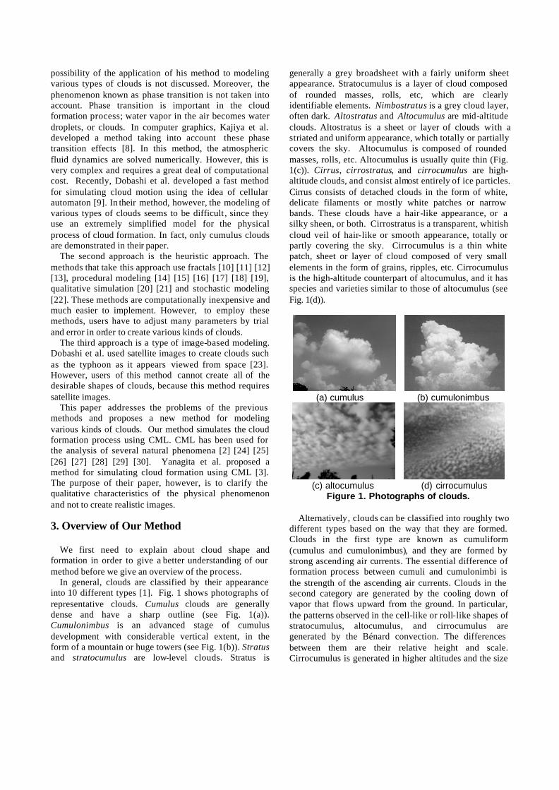
In our method, clouds are generated by simulating the cloud formation using a scheme employing CML. The simulation space is subdivided into three-dimensional lattices. Fig. 2 shows our system for cloud modeling/rendering. Firstly, the user specifies the types of clouds desired and the conditions for the simulation, i.e. the number of lattices, initial-conditions, the boundary conditions and the parameters for the atmospheric properties such as the viscosity and diffusion coefficient. The cloud formation is simulated based on the specified conditions using CML. During the simulation, the distribution of the state values such as the temperature, velocity and density of the clouds are visualized at every time step. The user can change these conditions interactively to control the shape of the clouds.

For generating cumulus or cumulonimbus, the distribution of the ascending current and source of humidity are specified, and then the velocity distribution and humidity distribution are calculated using CML method. The humid air moves upward due to the ascending currents during the calculation. As a result, clouds are formed by the phase transition. If we want to generate layer-like cloud formations we simulate the Bénard convection by inputting the difference in the temperature in the vertical direction and generate clouds by using the calculated velocity field.

After the simulation, we generate metaballs at the lattice points in order to render the clouds. The center density of each metaball is set to the density of the cloud particles in the corresponding lattice. Then, images of the clouds are generated by using the hardware-accelerated rendering method proposed by Dobashi et al. [9]. Many methods for rendering clouds have been proposed, and some of them take into account multiple scattering [5][8][13][31]. However, the main topic of this paper is the modeling of cloud shapes, so it is enough for us to consider only single scattering for a check on the cloud shape. Therefore, we decided to use Dobashi’s method since it is a method that can create images very quickly.

user interaction

atomospheric properties & boundary conditions

CML simulation rendering

inner state visualization

Figure 2. Our system for modeling/rendering clouds.

4. Simulation of Cloud Formation Using CML

We first explain the concept of the coupled map lattice (CML), and then propose a simulation method for cloud formation. 4.1 Coupled Map Lattice

CML is an extension of cellular automaton, and the simulation space is subdivided into lattices. Each lattice has several state variables, and their status is updated depending on the variables on the adjacent lattices. The main difference between CML and cellular automaton is in the state of the variables. CML uses real-value variables, while cellular automaton uses discrete variables.

The advantages of the CML approach are as follows. (1) The computational cost is small. (2) It is suitable for parallel processing. (3) A small number of lattices are sufficient to give qualitative simulations. 4.2 Modeling of Cloud Formation

To simulate fluid flow we have to consider the pressure, the density and the viscosity of the fluid. The atmosphere is a kind of compressible fluid, and its density changes depending on time and space. However, this change is very small, so we can assume that it is incompressible. Let us denote the velocity vector as v, the pressure as p , the density as ρ and the coefficient of viscosity as ν , so the Navier-Stokes equations are expressed as

.0

,1

=

∆+−=

v

vv

div

pgradDtD ν

ρ (1)

The second term of the above equation is called the “continuity equation”, meaning that it expresses the conservation of mass. The term DtDv is a material

derivative operator. Eq. (1) can be solved by numerical techniques, such as

the finite difference method. However, this is very time-consuming. In CML method, different approximated models are constructed. The models are computationally less than numerical techniques for solving the Navier-Stokes equations. The numerical model of cloud formation for CML is described below.

The simulation space is subdivided into lattices (see Fig. 3). The number of lattices is Nx× Ny× Nz. Clouds are formed as a bubble of air is heated by the underlying terrain, causing the bubble to rise into regions of low temperature. The phenomenon known as phase transition then occurs, that is, water vapor in the bubble becomes water droplets, or clouds. Therefore, the following factors have to be taken into account. (1) Viscosity and pressure

effects, (2) the advection of the state values by the fluid flow, (3) diffusion of water vapor, (4) thermal diffusion, (5) thermal buoyancy, (6) the phase transition from vapor to water. To simulate these factors, the velocity vector

),,( zyxv , the water vapor wv(x, y, z), the water droplets wl(x, y, z), and the temperature (or the internal energy)

),,( zyxE are defined at each lattice point, where x , y and z are integer values ( ,0 ,0 yx NyNx ≤≤≤≤ zNz ≤≤0 ).

Cloud formation is simulated by applying the processes described above for each time step. Parameters such as viscosity ratio described below for the simulation are constant over the simulation space. The numbers of lattices ),,( zyx NNN also affects the simulation result.

Each factor is formulated as follows. (1) Viscosity and Pressure Effect

The viscosity effect causes velocity diffusion. The pressure effect requires the concept of the conservation of mass, that is, the pressure term requires vdiv to be 0, the incompressible fluid. We do not use this condition here, since the inclusion of pressure variables requires more complicated modeling, and so often makes it difficult to construct a model using only local interactions. Instead, we introduce the discrete version of )( vdivgrad . vdiv is the mass flow of each lattice and )( vdivgrad is the flow caused by the gradient of the mass flow around lattices. The gradient of the pressure term, which depends on the velocity field, gives rise to a change of the velocity field. Let

xv be the x component of the velocity v for the

current time step and *xv be the x component of v for the

next time step. *xv is calculated from the following

equation (Note that the y and z components are calculated in a similar way).

,)(),,(),,(),,(*xpxvxx divgradkzyxvkzyxvzyxv v+∆+= (2)

where vk is the viscosity ratio and

pk is the coefficient of

the pressure effect. The second and the third terms are

)),,,(6 )1,,( )1,,(),1,(),1,(

),,1(),,1((61),,(

zyxvzyxvzyxvzyxvzyxv

zyxvzyxvzyxv

xx

xxx

xxx

−−+++−+++

−++=∆

(3)

( ) [ ]

1)].,1,(1),1,(

1),1,(1),1,()1,1,(

)1,1,( )1,1,()1,1,([41

),,(2),1,(),1,(21

−+−+−−

−−++++−+−

+−−−−++++

−−++=

zyxvzyxv

zyxvzyxvzyxv

zyxvzyxvzyxv

zyxvzyxvzyxvdivgrad

zz

zzy

yyy

xxxxv (4)

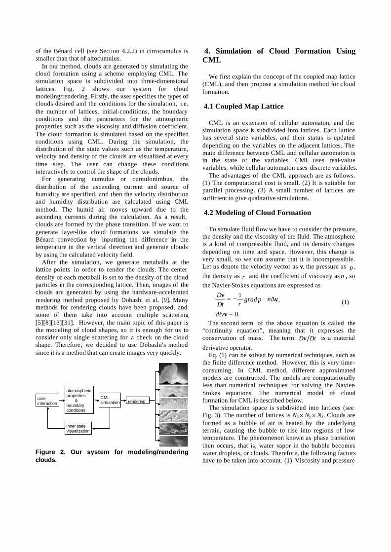
(2) Advection The state values at the lattice point ),,( zyx are

transported to a new position ),,( zyx vzvyvx +++ =

),,( znymxl δδδ +++ after updating the velocity v by using the equations described above, where l, m, n are the integer portions and xδ , yδ , zδ are the fractional portions

of xvx + ,

yvy + , zvz + . The values are then distributed

to the adjacent lattices. As shown in Fig. 3, let eight adjacent lattices be ),,( nml , ),,1( nml + , ),1,( nml + ,

),1,1( nml ++ , )1,,( +nml , )1,,1( ++ nml , 1)n1,,( ++ml and )1,1,1( +++ nml and let xδ be the distance between the new position and the lattice ),,( nml in the x direction,

yδ be the distance in the y direction, and zδ be the distance in the z direction. The weighted state values are added to these eight lattices with weights of

)1)(1)(1( zyx δδδ −−− , )1)(1( zyx δδδ −− , yx δδ )(1 −

)(1 zδ− , )1( zyx δδδ − , zyx δδδ )1)(1( −− , zyx δδδ )1( − ,

zyx δδδ )1( − and zyx δδδ , respectively. It is possible that the simulation is unstable if the

following condition is not satisfied. 0.1,, <zyx vvv . (5)

To address this problem, we tried to combine the advection part of Stam’s method [7] with ours. His method is stable even if Condition (5) is not satisfied. However, in our experiments, cloud-like shapes are not formed under the conditions which do not satisfy Condition (5) in our lattice size (see Section 5). We also investigated the range of parameters including velocities for getting a cloud-like shape, and we found that we need not apply the advection part of Stam’s method.

(l, m, n)

(l+1, m, n)

(l, m+1, n)

(l, m, n+1)

m+δy

l+δx

n+δz

Figure 3. Advection process.

(3) Diffusion of Water Vapor

Diffusion of water vapor ),,( zyxwv is modeled by

using a discrete version of the diffusion equation, i.e.

),,,(),,(),,( ,* zyxwkzyxwzyxw vwdvv ∆+= (6)

where wdk ,

is the diffusion coefficient for water vapor.

vw∆ is the difference of the water vapor per time step, and

is calculated in the same manner as in Eq. (3).

(4) Thermal Diffusion Thermal diffusion is simulated by the discrete version

of the diffusion equation. Thus the following equation is obtained.

),,(),,(),,( ,* zyxEkzyxEzyxE Ed

∆+= , (7)

where Edk ,

is the coefficient of thermal diffusion and E∆

is the difference in the temperature per time, and is calculated in the same manner as in Eq. (3). (5) Buoyancy

A lattice with higher temperature is subjected to a force in the upward direction. This results in an increase in the z component of the velocity of the lattice. We assume that the vertical velocity is incremented in proportion to the temperature difference between the lattice and its horizontal adjacent lattices. Therefore, the buoyancy effect is simulated by the following equation.

)}.,1,(),1,(),,1(

),,1(),,(4{4

),,(),,(*

zyxEzyxEzyxE

zyxEzyxEkzyxvzyxv bzz

−−+−−−

+−+= (8)

where bk is the coefficient affecting the strength of the

buoyancy force. We have tried other equations including the vertical direction. But so far as we have experimented, Eq. (8) fits best with known results on the actual phenomena. (6) Phase Transition

The amount of water droplets generated by the phase transition is determined in proportion to the difference between the maximum amount of water vapor and the amount of water vapor in each lattice. The maximum amount of water vapor for a unit volume of air is a function of its temperature (see appendix for details ). 4.2.1 Cumulus and Cumulonimbus

y x

z

vapor source

air current

cloud

Ny Nx

Nz

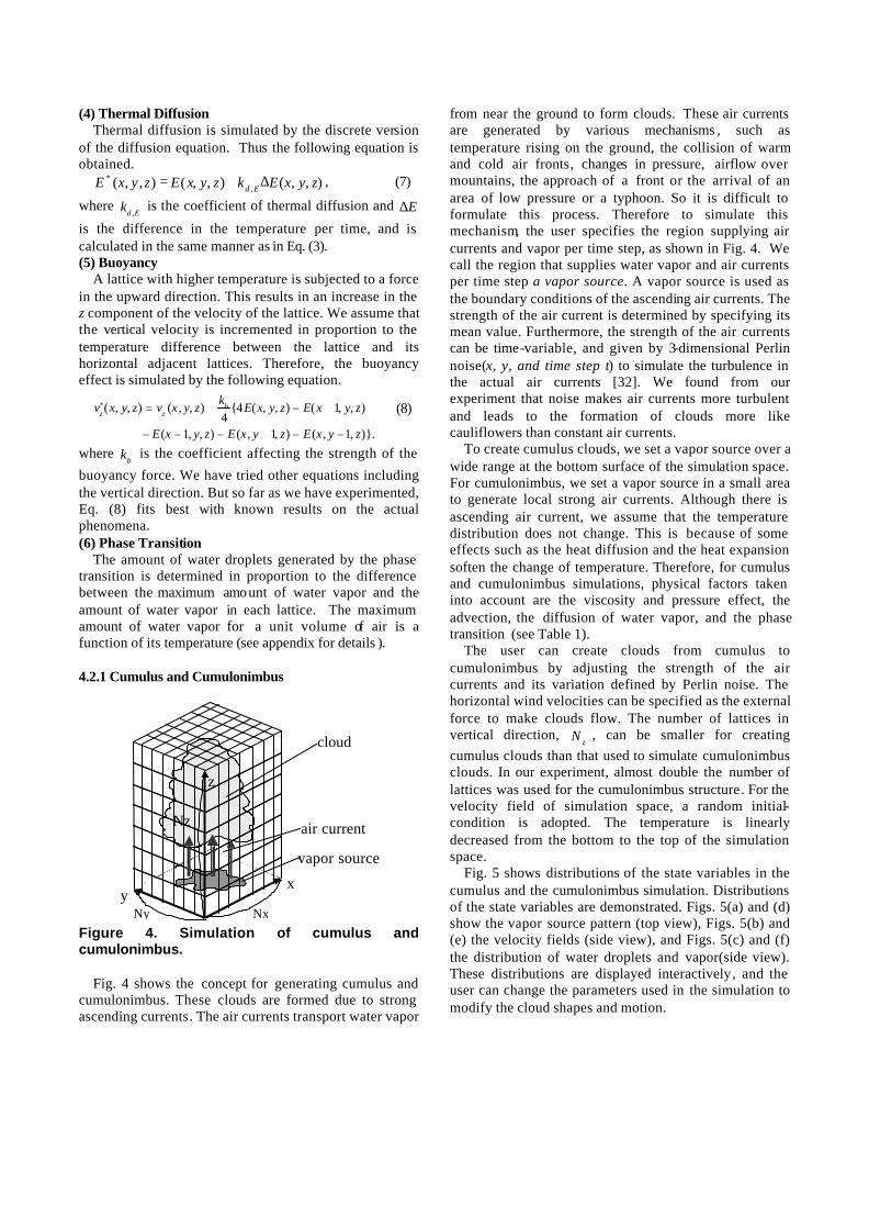
Figure 4. Simulation of cumulus and cumulonimbus.

Fig. 4 shows the concept for generating cumulus and cumulonimbus. These clouds are formed due to strong ascending currents. The air currents transport water vapor

from near the ground to form clouds. These air currents are generated by various mechanisms , such as temperature rising on the ground, the collision of warm and cold air fronts, changes in pressure, airflow over mountains, the approach of a front or the arrival of an area of low pressure or a typhoon. So it is difficult to formulate this process. Therefore to simulate this mechanism, the user specifies the region supplying air currents and vapor per time step, as shown in Fig. 4. We call the region that supplies water vapor and air currents per time step a vapor source. A vapor source is used as the boundary conditions of the ascending air currents. The strength of the air current is determined by specifying its mean value. Furthermore, the strength of the air currents can be time-variable, and given by 3-dimensional Perlin noise(x, y, and time step t) to simulate the turbulence in the actual air currents [32]. We found from our experiment that noise makes air currents more turbulent and leads to the formation of clouds more like cauliflowers than constant air currents.

To create cumulus clouds, we set a vapor source over a wide range at the bottom surface of the simulation space. For cumulonimbus, we set a vapor source in a small area to generate local strong air currents. Although there is ascending air current, we assume that the temperature distribution does not change. This is because of some effects such as the heat diffusion and the heat expansion soften the change of temperature. Therefore, for cumulus and cumulonimbus simulations, physical factors taken into account are the viscosity and pressure effect, the advection, the diffusion of water vapor, and the phase transition (see Table 1).

The user can create clouds from cumulus to cumulonimbus by adjusting the strength of the air currents and its variation defined by Perlin noise. The horizontal wind velocities can be specified as the external force to make clouds flow. The number of lattices in vertical direction,

zN , can be smaller for creating cumulus clouds than that used to simulate cumulonimbus clouds. In our experiment, almost double the number of lattices was used for the cumulonimbus structure. For the velocity field of simulation space, a random initial-condition is adopted. The temperature is linearly decreased from the bottom to the top of the simulation space.

Fig. 5 shows distributions of the state variables in the cumulus and the cumulonimbus simulation. Distributions of the state variables are demonstrated. Figs. 5(a) and (d) show the vapor source pattern (top view), Figs. 5(b) and (e) the velocity fields (side view), and Figs. 5(c) and (f) the distribution of water droplets and vapor(side view). These distributions are displayed interactively, and the user can change the parameters used in the simulation to modify the cloud shapes and motion.

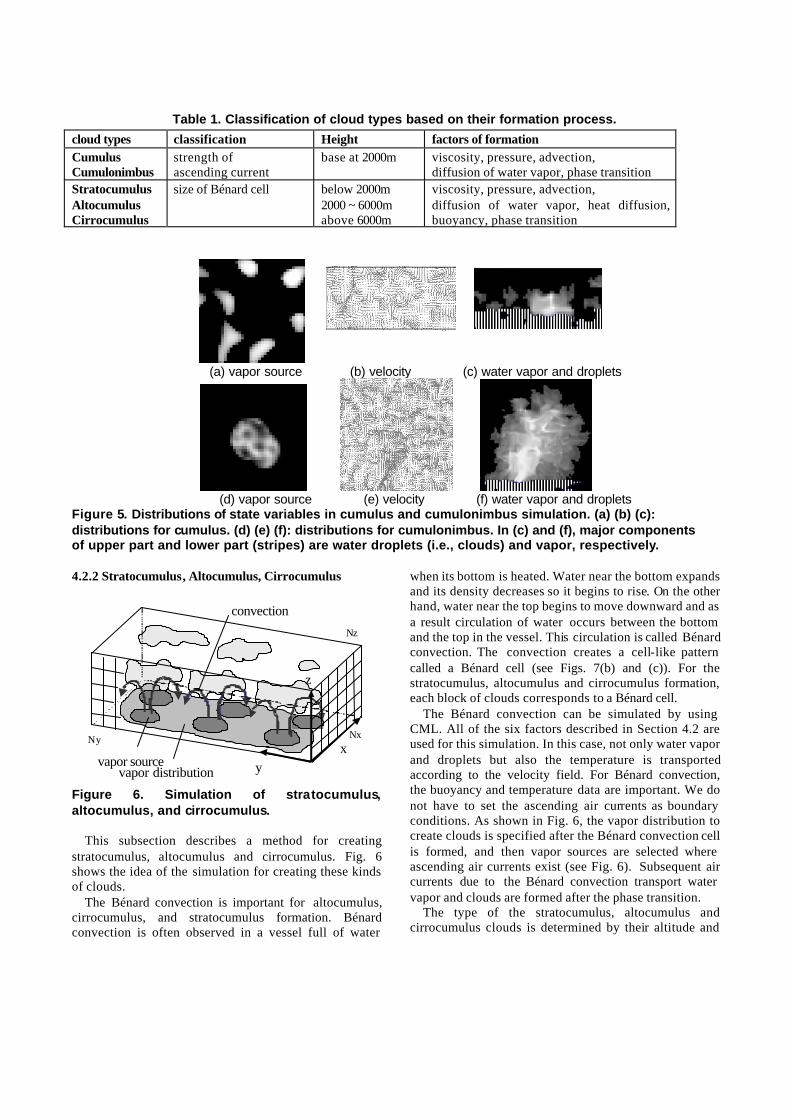
Table 1. Classification of cloud types based on their formation process.

(a) vapor source (b) velocity (c) water vapor and droplets

(d) vapor source (e) velocity (f) water vapor and droplets Figure 5. Distributions of state variables in cumulus and cumulonimbus simulation. (a) (b) (c): distributions for cumulus. (d) (e) (f): distributions for cumulonimbus. In (c) and (f), major components of upper part and lower part (stripes) are water droplets (i.e., clouds) and vapor, respectively. 4.2.2 Stratocumulus, Altocumulus, Cirrocumulus

vapor source

convection

vapor distribution

x

z

y

Nz

Nx Ny

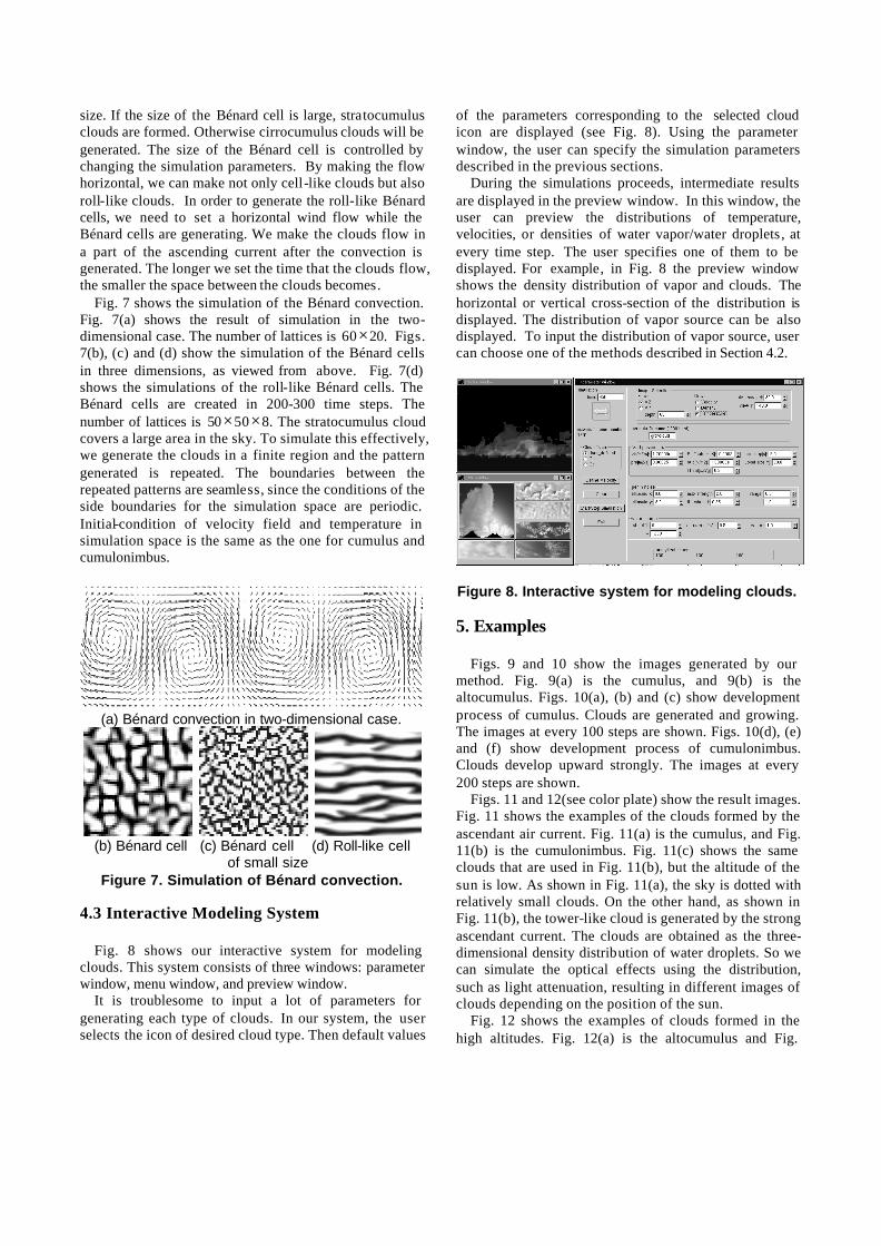
Figure 6. Simulation of stratocumulus, altocumulus, and cirrocumulus.

This subsection describes a method for creating stratocumulus, altocumulus and cirrocumulus. Fig. 6 shows the idea of the simulation for creating these kinds of clouds.

The Bénard convection is important for altocumulus, cirrocumulus, and stratocumulus formation. Bénard convection is often observed in a vessel full of water

when its bottom is heated. Water near the bottom expands and its density decreases so it begins to rise. On the other hand, water near the top begins to move downward and as a result circulation of water occurs between the bottom and the top in the vessel. This circulation is called Bénard convection. The convection creates a cell-like pattern called a Bénard cell (see Figs. 7(b) and (c)). For the stratocumulus, altocumulus and cirrocumulus formation, each block of clouds corresponds to a Bénard cell.

The Bénard convection can be simulated by using CML. All of the six factors described in Section 4.2 are used for this simulation. In this case, not only water vapor and droplets but also the temperature is transported according to the velocity field. For Bénard convection, the buoyancy and temperature data are important. We do not have to set the ascending air currents as boundary conditions. As shown in Fig. 6, the vapor distribution to create clouds is specified after the Bénard convection cell is formed, and then vapor sources are selected where ascending air currents exist (see Fig. 6). Subsequent air currents due to the Bénard convection transport water vapor and clouds are formed after the phase transition.

The type of the stratocumulus, altocumulus and cirrocumulus clouds is determined by their altitude and

cloud types classification Height factors of formation Cumulus Cumulonimbus

strength of ascending current

base at 2000m viscosity, pressure, advection, diffusion of water vapor, phase transition

Stratocumulus Altocumulus Cirrocumulus

size of Bénard cell below 2000m 2000 ~ 6000m above 6000m

viscosity, pressure, advection, diffusion of water vapor, heat diffusion, buoyancy, phase transition

size. If the size of the Bénard cell is large, stratocumulus clouds are formed. Otherwise cirrocumulus clouds will be generated. The size of the Bénard cell is controlled by changing the simulation parameters. By making the flow horizontal, we can make not only cell-like clouds but also roll-like clouds. In order to generate the roll-like Bénard cells, we need to set a horizontal wind flow while the Bénard cells are generating. We make the clouds flow in a part of the ascending current after the convection is generated. The longer we set the time that the clouds flow, the smaller the space between the clouds becomes.

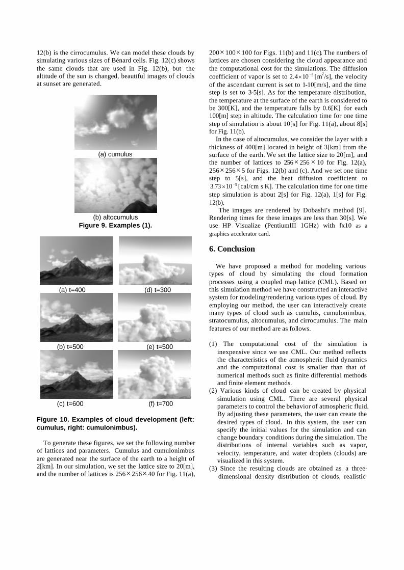
Fig. 7 shows the simulation of the Bénard convection. Fig. 7(a) shows the result of simulation in the two-dimensional case. The number of lattices is 60×20. Figs. 7(b), (c) and (d) show the simulation of the Bénard cells in three dimensions, as viewed from above. Fig. 7(d) shows the simulations of the roll-like Bénard cells. The Bénard cells are created in 200-300 time steps. The number of lattices is 50×50×8. The stratocumulus cloud covers a large area in the sky. To simulate this effectively, we generate the clouds in a finite region and the pattern generated is repeated. The boundaries between the repeated patterns are seamless, since the conditions of the side boundaries for the simulation space are periodic. Initial-condition of velocity field and temperature in simulation space is the same as the one for cumulus and cumulonimbus.

(a) Bénard convection in two-dimensional case.

(b) Bénard cell (c) Bénard cell (d) Roll-like cell

of small size Figure 7. Simulation of Bénard convection.

4.3 Interactive Modeling System

Fig. 8 shows our interactive system for modeling clouds. This system consists of three windows: parameter window, menu window, and preview window.

It is troublesome to input a lot of parameters for generating each type of clouds. In our system, the user selects the icon of desired cloud type. Then default values

of the parameters corresponding to the selected cloud icon are displayed (see Fig. 8). Using the parameter window, the user can specify the simulation parameters described in the previous sections.

During the simulations proceeds, intermediate results are displayed in the preview window. In this window, the user can preview the distributions of temperature, velocities, or densities of water vapor/water droplets, at every time step. The user specifies one of them to be displayed. For example, in Fig. 8 the preview window shows the density distribution of vapor and clouds. The horizontal or vertical cross-section of the distribution is displayed. The distribution of vapor source can be also displayed. To input the distribution of vapor source, user can choose one of the methods described in Section 4.2.

Figure 8. Interactive system for modeling clouds. 5. Examples

Figs. 9 and 10 show the images generated by our method. Fig. 9(a) is the cumulus, and 9(b) is the altocumulus. Figs. 10(a), (b) and (c) show development process of cumulus. Clouds are generated and growing. The images at every 100 steps are shown. Figs. 10(d), (e) and (f) show development process of cumulonimbus. Clouds develop upward strongly. The images at every 200 steps are shown.

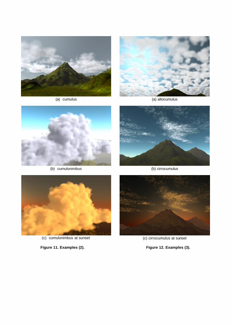
Figs. 11 and 12(see color plate) show the result images. Fig. 11 shows the examples of the clouds formed by the ascendant air current. Fig. 11(a) is the cumulus, and Fig. 11(b) is the cumulonimbus. Fig. 11(c) shows the same clouds that are used in Fig. 11(b), but the altitude of the sun is low. As shown in Fig. 11(a), the sky is dotted with relatively small clouds. On the other hand, as shown in Fig. 11(b), the tower-like cloud is generated by the strong ascendant current. The clouds are obtained as the three-dimensional density distribution of water droplets. So we can simulate the optical effects using the distribution, such as light attenuation, resulting in different images of clouds depending on the position of the sun.

Fig. 12 shows the examples of clouds formed in the high altitudes. Fig. 12(a) is the altocumulus and Fig.

12(b) is the cirrocumulus. We can model these clouds by simulating various sizes of Bénard cells. Fig. 12(c) shows the same clouds that are used in Fig. 12(b), but the altitude of the sun is changed, beautiful images of clouds at sunset are generated.

(a) cumulus

(b) altocumulus

Figure 9. Examples (1).

(a) t=400 (d) t=300

(b) t=500 (e) t=500

(c) t=600 (f) t=700

Figure 10. Examples of cloud development (left: cumulus, right: cumulonimbus).

To generate these figures, we set the following number of lattices and parameters. Cumulus and cumulonimbus are generated near the surface of the earth to a height of 2[km]. In our simulation, we set the lattice size to 20[m], and the number of lattices is 256× 256× 40 for Fig. 11(a),

200× 100× 100 for Figs. 11(b) and 11(c). The numbers of lattices are chosen considering the cloud appearance and the computational cost for the simulations. The diffusion coefficient of vapor is set to 5104.2 −× [m2/s], the velocity of the ascendant current is set to 1-10[m/s], and the time step is set to 3-5[s]. As for the temperature distribution, the temperature at the surface of the earth is considered to be 300[K], and the temperature falls by 0.6[K] for each 100[m] step in altitude. The calculation time for one time step of simulation is about 10[s] for Fig. 11(a), about 8[s] for Fig. 11(b).

In the case of altocumulus, we consider the layer with a thickness of 400[m] located in height of 3[km] from the surface of the earth. We set the lattice size to 20[m], and the number of lattices to 256× 256 × 10 for Fig. 12(a), 256× 256× 5 for Figs. 12(b) and (c). And we set one time step to 5[s], and the heat diffusion coefficient to

51073.3 −× [cal/cm s K]. The calculation time for one time step simulation is about 2[s] for Fig. 12(a), 1[s] for Fig. 12(b).

The images are rendered by Dobashi’s method [9]. Rendering times for these images are less than 30[s]. We use HP Visualize (PentiumIII 1GHz) with fx10 as a graphics accelerator card. 6. Conclusion

We have proposed a method for modeling various types of cloud by simulating the cloud formation processes using a coupled map lattice (CML). Based on this simulation method we have constructed an interactive system for modeling/rendering various types of cloud. By employing our method, the user can interactively create many types of cloud such as cumulus, cumulonimbus, stratocumulus, altocumulus, and cirrocumulus. The main features of our method are as follows. (1) The computational cost of the simulation is

inexpensive since we use CML. Our method reflects the characteristics of the atmospheric fluid dynamics and the computational cost is smaller than that of numerical methods such as finite differential methods and finite element methods.

(2) Various kinds of cloud can be created by physical simulation using CML. There are several physical parameters to control the behavior of atmospheric fluid. By adjusting these parameters, the user can create the desired types of cloud. In this system, the user can specify the initial values for the simulation and can change boundary conditions during the simulation. The distributions of internal variables such as vapor, velocity, temperature, and water droplets (clouds) are visualized in this system.

(3) Since the resulting clouds are obtained as a three-dimensional density distribution of clouds, realistic

images of clouds can be displayed that take the light scattering due to cloud particles into account. Clouds are rendered efficiently by making use of graphics hardware.

References [1] R. A. Houze, “Cloud Dynamics”, International Geophysics

Series Vol.53, Academic Press, New York, 1993. [2] K. Kaneko, “Simulating Physics with Coupled Map

Lattices-Pattern Dynamics, Information Flow, and Thermodynamics of Spatiotemporal Chaos,” Vol. 1, World Scientific, Singapore, 1990.

[3] T. Yanagita and K. Kaneko, “Modeling and Characterization of Clouds Dynamics,” Phys. Rev. Lett., Vol. 78, No. 22, 1997, pp. 4297-4300.

[4] J. Stam, E. Fiume, “Turbulent Wind Fields for Gaseous Phenomena,” Proc. SIGGRAPH'93, 1993, pp. 369-376.

[5] J. Stam, E. Fiume, “Dipicting Fire and Other Gaseous Phenomena Using Diffusion Processes,” Proc. SIGGRAPH'95, 1995, pp. 129-136.

[6] N. Foster, D. Metaxas, “Modeling the Motion of a Hot, Turbulent Gas,” Proc. SIGGRAPH’97, 1997, pp. 181-188.

[7] J. Stam, “Stable Fluids,” Proc. SIGGRAPH'99, 1999, pp. 121-128.

[8] J. T. Kajiya, B. P. V. Herzen, “Ray Tracing Volume Densities,” Computer Graphics , 1984, Vol. 18, No. 3, pp. 165-174

[9] Y. Dobashi, K. Kaneda, H. Yamashita, T. Okita, T. Nishita, “A Simple, Efficient Method for Realistic Animation of Clouds,” Proc. SIGGRAPH2000, 2000, pp. 19-28.

[10] R. Voss, “Fourier Synthesis of Gaussian Fractals: 1/f noises, landscapes, and flakes,” Proc. SIGGRAPH’83: Tutorial on State of the Art Image Synthesis, 10, 1983.

[11] G.Y. Gardner, “Visual Simulation of Clouds,” Computer Graphics , Vol.19, No. 3, 1985, pp. 279-303.

[12] T. Nishita, S. Takao, T. Katsumi, E. Nakamae, “Display of The Earth Taking into Account Atmospheric Scattering,” Proc. SIGGRAPH’93, pp. 175-182 , 1993.

[13] T. Nishita, Y.Dobashi, E.Nakamae,"Display of Clouds Taking into Account Multiple Anisotropic Scattering and Sky Light," Proc. SIGGRAPH'96, 1996-8, pp.379-386.

[14] N. Max, “Light Diffusion through Clouds and Haze,” Graphics and Image Processing, Vol. 13, No. 3, 1986, pp. 280-292.

[15] D. S. Ebert, R. E. Parent, “Rendering and Animation of Gaseous Phenomena by Combining Fast Volume and Scanline A-Buffer Techniques,” Computer Graphics , Vol. 24, No. 4, 1990, pp. 357-366.

[16] D. S. Ebert, W. E. Carlson, R. E. Parent, “Solid Spaces and Inverse Particle Systems for Controlling the Animation of Gases and Fluids,” The Visual Computer , 10, 1990, pp. 471-483.

[17] D. S. Ebert, “Volumetric Modeling with Implicit Functions: A Cloud is Born,” Visual Proc. SIGGRAPH’97, 1997, pp. 147.

[18] D. S. Ebert, “Simulating Nature: From Theory to Application,” Course Note #26 of SIGGRAPH’99, 1999, pp. 5.1-5.52.

[19] N. Max, R. Crawfis, D. Williams, “Visualizing Wind Velocities by Advecting Cloud Textures,” Proc. Visualization’92, 1992, pp. 179-183.

[20] T. Kikuchi, K. Muraoka, and N. Chiba, “Visual Simulation of Cumulonimbus Clouds,” The Journal of The Institute of Image Electronics and Electronics Engineers of Japan, Vol. 27, No. 4, 1998, pp. 317-326 (in Japanese).

[21] F. Neyret, “Qualitative Simulation of Convective Clouds Formation and Evolution,” EGCAS’97, 1997, pp. 113-124.

[22] J. Stam, “Stochastic Rendering of Density Fields,” Proc. Graphics Interface’94, 1994, pp. 51-58.

[23] Y. Dobashi, T. Nishita, H. Yamashita, T. Okita, “Using Metaballs to Modeling and Animate Clouds from Satellite Images,” The Visual Computer , Vol. 15, No. 9, 1998, pp. 471-482.

[24] Y. Oono and S. Puri, “Computationally Efficient Modeling of Ordering of Quenched Phases,” Phys. Rev. Lett., Vol. 58, No. 8, 1987, pp.836-839.

[25] A. Shinozaki and Y. Oono, “Cell Dynamical Systems,” Forma, 4, 1989, pp. 75-102.

[26] H. Nirhimori and Y. Oobuchi, “Formation of Ripple Patterns and Dunes by Wind-blown sand,” Phys. Rev. Lett., Vol. 71, 1993, pp. 197.

[27] T. Yanagita, “Coupled Map Lattice Model for Boiling,” Phys. Lett. A, 165, 1992, pp. 405-408.

[28] T. Yanagita, “Phenomenology for Boiling: A Coupled Map Lattice Model,” Chaos, Vol. 3, No. 2, 1992, pp. 343.

[29] T. Yangita and K. Kaneko, “Coupled Map Lattice Model for Convection,” Phys. Lett. A, Vol. 175, 1993, pp. 415-420.

[30] T. Yanagita and K. Kaneko, “Rayleigh-Benard Convection; Patters, Chaos, Spatiotemporal Chaos and Turbulent,” Physica D, Vol. 82, 1995, pp. 288-313.

[31] N. Max, “Efficient Light Propagation for Multiple Anisotropic Volume Scattering,” Proc. the Fifth Eurographics Workshop on Rendering, 1994, pp. 87-104.

[32] K. Perlin, “An Image Synthesizer,” Proc. SIGGRAPH'85, 1985, pp. 287-296.

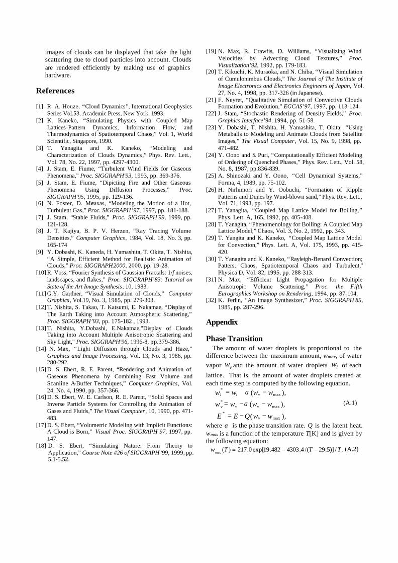
Appendix Phase Transition

The amount of water droplets is proportional to the difference between the maximum amount, wmax, of water vapor vw and the amount of water droplets lw of each

lattice. That is, the amount of water droplets created at each time step is computed by the following equation.

),(

),(

),(

max*

max*

max*

wwQEE

wwww

wwww

v

vvv

vll

−−=

−−=

−+=

α

α (A.1)

where α is the phase transition rate. Q is the latent heat. wmax is a function of the temperature T[K] and is given by the following equation:

./)]5.29/(4.4303482.19exp[0.217)(max TTTw −−= (A.2)

(a) cumulus

(b) cumulonimbus

(c) cumulonimbus at sunset

(a) altocumulus

(b) cirrocumulus

(c) cirrocumulus at sunset

Figure 11. Examples (2). Figure 12. Examples (3).