a optimal and robust mechanism design with …theory.stanford.edu/~tim/papers/interdependent.pdfwe...

A

Optimal and Robust Mechanism Design with Interdependent Values

TIM ROUGHGARDEN, Stanford UniversityINBAL TALGAM-COHEN, Stanford University

We study interdependent value settings [Milgrom and Weber 1982] and extend several fundamental resultsfrom the well-studied independent private values model to these settings. For revenue-optimal mechanismdesign, we give conditions under which Myerson’s virtual value-based mechanism remains optimal withinterdependent values. One of these conditions is robustness of the truthfulness and individual rationalityguarantees, in the sense that they are required to hold ex post. We then consider an even more robust classof mechanisms called “prior independent” (a.k.a. “detail free”), and show that by simply using one of thebidders to set a reserve price, it is possible to extract near-optimal revenue in an interdependent valuessetting. This shows that a considerable level of robustness is achievable for interdependent values in single-parameter environments.

Categories and Subject Descriptors: [Theory of Computation]: General

General Terms: Algorithms, Economics, Theory

Additional Key Words and Phrases: interdependence; correlated values; optimal auctions; Myerson theory;prior-independence

1. INTRODUCTIONThe subject of this paper is optimal and robust mechanism design in the classic modelof interdependent values introduced by Milgrom and Weber [1982]. The model of inter-dependent values is not only of economic importance in itself, but also sheds new lighton the inherent tradeoff between revenue maximization and robustness in the designof mechanisms.

In technical terms, we study optimal and approximately-optimal mechanisms insingle-parameter settings, with robust guarantees of ex post incentive compatibilityand individual rationality; the approximately-optimal mechanisms we design are alsoprior-independent, that is, robust to distributional details.

1.1. IPV versus Interdependent ValuesEconomic research on auctions has explored different valuation models over the pastdecades, which can roughly be divided into independent private1 values (IPV), versus

1The term “private” is used here as opposed to “common”, not to be confused with private in the sense of“non-public”, as in the context of information asymmetries. In what follows to avoid confusion we shall referto non-public information as “privately-known”.

This research was supported in part by NSF Awards CCF-1016885 and CCF-1215965 and an ONR PECASEAward. The second author is supported by the Hsieh Family Stanford Interdisciplinary Graduate Fellowship.Author’s addresses: T. Roughgarden and I. Talgam-Cohen, Computer Science Department, Stanford Univer-sity, Stanford, CA 94305 USA.An earlier version of this work appeared in the 14th ACM Conference on Economics and Computation(EC’13; formerly known as ACM Conference on Electronic Commerce), 2013.Permission to make digital or hard copies of part or all of this work for personal or classroom use is grantedwithout fee provided that copies are not made or distributed for profit or commercial advantage and thatcopies show this notice on the first page or initial screen of a display along with the full citation. Copyrightsfor components of this work owned by others than ACM must be honored. Abstracting with credit is per-mitted. To copy otherwise, to republish, to post on servers, to redistribute to lists, or to use any componentof this work in other works requires prior specific permission and/or a fee. Permissions may be requestedfrom Publications Dept., ACM, Inc., 2 Penn Plaza, Suite 701, New York, NY 10121-0701 USA, fax +1 (212)869-0481, or [email protected]© YYYY ACM 1539-9087/YYYY/01-ARTA $10.00

DOI 10.1145/0000000.0000000 http://doi.acm.org/10.1145/0000000.0000000

ACM Transactions on Embedded Computing Systems, Vol. V, No. N, Article A, Publication date: January YYYY.

A:2 T. Roughgarden and I. Talgam-Cohen

the more general class of interdependent values that allows for correlation and com-monality (see [Krishna 2010, Chapters 2-5; 13-17] versus [Krishna 2010, Chapters6-10; 18]). The more nacent research effort in theoretical computer science has focusedlargely on the more restricted IPV model, recently also venturing into the realm ofcorrelation (see, notably, [Papadimitriou and Pierrakos 2011; Dobzinski et al. 2011;Cai et al. 2012]). A broad research goal is therefore to apply the computer science lensto the study of mechanisms for the general interdependent model. This paper takesfirst steps in that direction by unifying and generalizing previous results to establishthe necessary technical foundation, and demonstrates that there are natural sufficientconditions under which positive results in the form of mechanisms with very strongguarantees can be achieved.

The importance of the interdependent model in the economic literature stems fromthe fact that for many high-stake auctions that arise in practice, interdependent val-ues are a more realistic model of bidders’ values than IPV. Interdependence capturessituations in which every bidder has only partial information, called his signal, abouthis value for winning the auction, and this information can be correlated with otherbidders’ information. Furthermore, the information held by other bidders may directlyaffect the bidder’s value – mathematically his value is a function of his own signal andthe (possibly correlated) signals of his competitors.

A classic example from the economic literature is the mineral rights model [Wilson1969]. In auctions for oil drilling, the value of the drilling rights is determined bywhether or not there is oil to be found on the drilling site. This value is often common– yet unknown – to all bidders. However, typically every bidder has some private noisysignal regarding the value, achieved by, for example, conducting a geological survey.Not only are these signals positively correlated, but the information gathered by theother bidders would certainly change a bidder’s expected value for winning if he gainedaccess to it.

Note that the IPV model is not rich enough to capture the described informationalsetting: In the IPV model an attempted approximation is that values all come from adistribution over a high-valued support (oil exists), or a low-valued one (no oil). But tomodel that the seller does not know which of the two supports is the case will makethe bidders correlated in his view. Similarly, we need interdependence to model thatbidders do not know their precise value for winning an auction since it depends onothers’ information. The model of interdependence thus enriches the set of underlyingassumptions we are able to make about the informational structure of the auctionsetting. In this paper we explicitly treat such informational assumptions and theirrole in designing mechanisms, as discussed next.

1.2. Robustness in Mechanism DesignA second goal of this paper is the design of robust mechanisms. Consider the informa-tional assumptions of a standard Bayesian auction environment, where bidders haveprivately-known information.

Informational assumption 1. The bidders all know the probability distribution of theprivately-known information, and make strategic decisions accordingly.

Informational assumption 2. The seller knows the probability distribution of theprivately-known information, and chooses the mechanism (or sets parameters suchas reserve prices) accordingly.

There are many theoretical and practical reasons to wish to relax the above as-sumptions; for example, accurate prior information may be expensive to acquire, ora mechanism may need to be re-used in settings with different distributions. In fact,


Optimal and Robust Mechanism Design with Interdependent Values A:3

Table I. Terminology. The term interdependent values encompasses all four value classesdescribed in the table.

Private Non-private (common)Independent Independent private values (IPV) Non-private valuesCorrelated Correlated values Correlated non-private values

the issue of robustness to informational assumptions as above is “an old theme in themechanism design literature” [Bergemann and Morris 2005] (see further discussion inSection 3.2 below). However, potentially there can be a trade-off between robustnessand the objectives of the mechanism, in our case maximizing revenue.

Remarkably, Myerson [1981] showed that in the IPV model there is no trade-off withrespect to the first assumption:2 The optimal mechanism among all mechanisms thatmake assumption 1 does not actually use this assumption in any way. More formally,Myerson’s optimal mechanism is ex post incentive compatibile (IC) and individuallyrational (IR), but is optimal among all Bayesian IC and interim IR mechanisms (seeSection 3.1 for definitions of these solution concepts).

On the other hand, in the context of interdependent values, the trade-off not onlyexists but becomes very extreme. A mechanism making assumption 1 can extract asrevenue essentially the full welfare arising from the auction, leaving the bidders withvirtually zero utility from participation [Cremer and McLean 1985; 1988]. Intuitively,dependencies among the bidders “cancel out” their strategic advantage from privately-held information and nullifies their information rents. Without assumption 1 however,the gap between the optimal expected revenue and full welfare can be arbitrarily large.

While relaxing assumption 1 leads to a loss of revenue, a possibly surprising prop-erty is regained. It turns out that Myerson’s result [1981], showing the fundamentalconnection between the allocation and payment rules needed to induce truthfulness,extends to interdependent values once we restrict attention to mechanisms that areex post. We show that under conditions well-studied in the literature, it is possible tofollow the same path as in Myerson’s original paper and get an analogue of the Myer-son optimal mechanism for interdependent values, where optimality is among all expost mechanisms. This relates the goal of robustness to that of expanding the theoryfor interdependent values – the latter is made possible by imposing robustness as arequirement.

We now revisit the second informational assumption, and ask what is achievable forinterdependent values when both assumptions are relaxed. Even in the IPV model,the Myerson mechanism heavily depends on assumption 2. The question of designingnew mechanisms without this assumption has been studied in the IPV model, leadingto the theory of prior-independence. We give the first prior-independence result beyondthe IPV model; in particular we show that while interdependence does complicate theproblem of relaxing assumption 2, a considerable level of robustness is still achievablewithout giving up too much expected revenue.

1.3. Our ResultsThis paper makes two main technical contributions. To describe these and for the re-mainder of the paper we use the terminology in Table I.

(1) We develop a general analogue of Myerson’s optimal auction theory that appliesto many interdepedent settings of interest. While Myerson’s theory does not hold ingeneral for interdependent values (indeed, there are settings in which the Cremer-McLean mechanism extracts higher revenue than the Myerson mechanism), we showit is partially recovered when we impose ex post rather than Bayesian IC and IR con-

2For now we assume that the second assumption holds.



straints. This synthesizes and generalizes many known results in the economic litera-ture (see related work in Section 4).

We first apply standard techniques to characterize ex post IC and IR mechanismsin the interdependent model and to show that their expected revenue equals their ex-pected “conditional virtual surplus”. Notably, we use the characterization to identifysufficient conditions under which the simple, “ironless” form of the Myerson mecha-nism is optimal. Under these conditions, the optimal mechanism simply allocates tothe bidders with highest non-negative (conditional) virtual values.

(2) For non-private value settings we analyze a prior-independent auction and showthat it is simultaneously near-optimal across a range of possible prior distributions. Inparticular, we adapt the single sample approach of Dhangwatnotai et al. [2010] to inter-dependent values, and show that with an additional sufficient and necessary MHR as-sumption, this approach results in an approximately-optimal, prior-independent mech-anism.

Our prior-independence result demonstrates that non-trivial research questions canarise even in the simplest interdependent settings. Our Myerson-like characterizationsuggests that many interesting mechanism design results should be possible, evenwhen bidders have interdependent values.

1.4. OrganizationIn Sections 2 and 3 we present the model and the basic ex post solution concept. InSection 4 we survey related work. Section 5 develops the first result above and thesecond result appears in Section 6. The study of interdependent settings raises manyfurther research directions, several of which appear in Section 7.

2. MODEL2.1. Interdependent Values Model

Single-parameter environments. We consider single-parameter Bayesian auction en-vironments (E, I), where E = {1, . . . , n} is a set of bidders, and I ⊆ 2E is a non-emptycollection of feasible bidder subsets, i.e., subsets of bidders who can win the auctionsimultaneously. (E, I) is a downward-closed set system, in which a subset of a feasiblesubset is also feasible. A canonical example of a single-parameter environment is amulti-unit auction with unit-demand bidders, where I is all sets of bidders for whichthe number of bidders is at most the number of units. Our results are generally ofinterest even for single-item auctions.

Signals and interdependent values. The bidders have possibly correlated, privately-known signals s1, . . . , sn, drawn from a joint distribution F with density f over thesupport [0, ωi]

n (ωi may be ∞). We adopt the standard assumptions that f is continu-ous and nowhere zero. Every bidder i has a publicly-known valuation function vi whosearguments are the signals, and his interdependent value for winning is vi(~s). Interde-pendent values are also called information externalities among the bidders. When thebidders share the same valuation function we say they have a pure common value. Weimpose the following standard assumptions on the valuation function vi(·):

— Non-negative and normalized (vi(~0) = 0);— Twice continuously differentiable;— Non-decreasing in all variables, strictly increasing in si.— Finite expectation E~s[vi(~s)] <∞.

Encompassed value models. The described interdependent values model is very gen-eral; it includes several narrower settings of interest (recall Table I):



(1) Correlated values settings, in which vi(~s) = si for every i and the signals/valuesare correlated;

(2) Non-private values settings, in which the signals are independent (drawn indepen-dently from distributions {Fi}) and the valuation functions vi(~s) are general;

(3) Independent private values (IPV) settings, in which both vi(~s) = si for every i andthe signals/values are independent.

Notation. Fix a signal profile s−i. Let vi|s−i(·) denote bidder i’s value given s−i as a

function of his signal si. Since vi is strictly increasing in si, then vi|s−i(·) is invertible;

denote by v−1i|s−i(ν) or v−1i (ν | s−i) the signal si such that vi|s−i

(si) = ν. Slightly abusingnotation, given s−i denote the derivative of vi|s−i

(·) at si by

d

dsivi(~s) =

d

dsivi|s−i

(si).

2.2. Motivating ExamplesWe describe two natural and standard examples of non-private values. In the firstexample, bidders’ values directly depend on the private preferences of the others. Inthe second example, bidders’ values depend on a hidden stochastic “state of the world”,of which others may posses private knowledge. We then give an example of correlatedsignals.

Example 2.1 (Weighted-sum values). Let β ∈ [0, 1]. Every bidder’s value is a sum ofhis own signal and a weighted sum of the other signals:

vi(~s) = si + β∑j 6=i

sj .

This is a simplified version of Myerson’s value with revision effects [Myerson 1981],and when β = 1, this results in the wallet game [Klemperer 1998]. Weighted-sumvalues are a plausible value model for a painting sold in auction; a bidder’s value forthe painting is determined by his own appreciation of it, combined with the painting’s“resale value” based on how much others appreciate it.

Example 2.2 (Conditionally-independent values, a.k.a mineral rights model). Bid-ders have a hidden stochastic pure common value v, modeled by a random variableV drawn from a publicly known distribution FV . An important feature of the mineralrights model is that conditional on the event V = v, bidders’ signals are independent.Furthermore, each signal is an unbiased estimator of V (its expectation when V = vequals v). The bidders’ effective value – their value for all operational purposes – is thepure common value

vi(~s) = EV∼FV[V | ~s].

The mineral rights model was developed to capture values in auctions for oil drillingleases [Wilson 1969]. Such values are determined by the true amount of existing oil,but uncertainty and information asymmetries regarding this amount creates interde-pendency.

A concrete setting of interest is the one in which FV is distributed normally withparameters µV , σV (assume µV is far from 0 and σV is small), and the signals aresi = v+ ηi, where η1, . . . , ηn are i.i.d. samples drawn from the normal distribution withparameters µη = 0 and some small ση. In this case the value is a linear combination of



the prior and empirical means, similar to Example 2.1 above:

vi(~s) =nσ2

V

nσ2V + σ2

η

(1

n

∑i

si) +σ2η

nσ2V + σ2

η

µV .

Up to normalization, the coefficient of the empirical mean 1n

∑i si is the prior variance

and the coefficient of the prior mean µV is the noise variance.

Example 2.3 (Signals drawn from a multivariate normal distribution). The sig-nals in Example 2.1 above can be arbitrarily correlated. A concrete example of a jointsignal distribution is a symmetric multivariate normal distribution. This distributionis “nice” in the sense that its marginals are normal as well, and if all pairwise covari-ances are nonnegative, then signals drawn from it satisfy a strong form of correlationcalled affiliation. We will make use of these properties below.

2.3. Conditional Virtual Values and RegularityFix a bidder i and a signal profile s−i. The conditional marginal density fi(· | s−i) ofbidder i’s signal given s−i is

fi(si | s−i) =f(~s)∫ ωi

0f(t, s−i)dt

.

We denote the corresponding distribution by Fi(· | s−i). The conditional revenue curveBi(· | s−i) of bidder i is

Bi(si | s−i) = vi(~s)

∫ ωi

si

fi(t | s−i)dt.

The conditional revenue curve represents the expected revenue from setting a thresh-old price vi(si, s−i) for bidder i given that the other signals are s−i.3 We can now definethe conditional virtual value of bidder i as

ϕi(si | s−i) = −ddsiBi(si | s−i)fi(si | s−i)

= vi(~s)−1− Fi(si | s−i)fi(si | s−i)

· ddsi

vi(~s). (1)

For private values, the conditional virtual value simplifies to a more familiar form:

ϕi(si | s−i) = si −1− Fi(si | s−i)fi(si | s−i)

, (2)

For independent common values it simplifies to the form

ϕi(si | s−i) = vi(~s)−1− Fi(si)fi(si)

· ddsi

vi(~s). (3)

Regularity and MHR. We say that Fi(· | s−i) is regular if the conditional virtualvalue ϕi(· | s−i) is weakly increasing; we say it has monotone hazard rate, or MHR, ifthe inverse hazard rate (1−Fi(si | s−i))/fi(si | s−i) is weakly decreasing. Its monopolyprice is the signal si such that the conditional virtual value ϕi(si | s−i) equals zero.

Conditional vs. standard virtual values. Equation (1) reveals three complicationsintroduced by conditional virtual values in comparison to standard virtual values inthe IPV model: first, the value vi is a function of others’ signals s−i; second, the in-verse hazard rate is conditional on s−i; and third, there is an extra term dvi/dsi. The

3Equation 2.3 uses the assumption that vi is strictly increasing in si, so that the probability with whichbidder i’s value is at least vi(~s) equals the probability

∫ ωisi

fi(t | s−i)dt that bidder i’s signal is at least si.



Myerson-like mechanisms we study below will rank bidders according to their condi-tional virtual values; while in the IPV model regularity is sufficient for such a mecha-nism to be IC, these three complications suggest that assumptions beyond regularitywill be required. For example, regularity of the signal distribution restricts only theconditional marginals, whereas for a joint distribution more “global” constraints maybe necessary.

2.4. Auction Settings of InterestWe present several settings of particular interest which are extensively studied in theliterature. These settings arise by imposing natural further assumptions on a generalsingle-parameter auction environment, and we will repeatedly refer to them in ourresults.

2.4.1. Matroid settings. Matroid settings arise by imposing a “substitutes” structure onthe feasible bidder subsets. The non-empty, downward-closed system (E, I) of biddersand feasible subsets is a matroid if the following exchange property holds: for everyS, T ∈ I such that |S| > |T |, there is some bidder i ∈ S\T such that T ∪{i} ∈ I (see, e.g.,[Oxley 1992]). Examples of matroid settings include digital goods where I = 2E , k-unitauctions where I is all subsets of size at most k, and certain unit-demand matchingmarkets corresponding to transversal matroids.

2.4.2. Settings with regularity or MHR. Settings in which the signal distribution F is reg-ular (resp., MHR). That is, for every bidder i and signal profile s−i, the conditionalmarginal distribution Fi(· | s−i) is regular (resp., MHR). The multivariate normal dis-tribution in Example 2.3 is MHR and thus also regular. Regularity arises in the IPVsetting as a necessary condition for truthfulness of Myerson’s mechanism without anadditional ironing procedure.

2.4.3. Settings with affiliation. Settings which arise by imposing affiliation — a form ofpositive correlation — on the joint signal distribution F with density f . Affiliationwas introduced by Milgrom and Weber [1982] and since then has become a standardassumption in the context of correlated and interdependent values, so much so that itis considered “almost synonymous with dependence in auctions.” [de Castro 2010]. Itis related to many well-studied mathematical concepts such as association, the FKGinequality and log-supermodularity [Alon and Spencer 2008].

Intuitively, signals are affiliated when observing a subset of high signals makes itmore likely that the remaining signals are also high. Formally, for every pair of signalprofiles ~s,~t ∈ [0, ωi]

n it must hold that

f(~s ∨ ~t)f(~s ∧ ~t) ≥ f(~s)f(~t), (4)

where (~s ∨ ~t) is the component-wise maximum, and (~s ∧ ~t) is the component-wise min-imum. Note that the inequality in (4) holds with equality for independent signals. Italso holds for the multivariate normal distribution in Example 2.3, which is affiliatedsince all pairwise covariances are nonnegative [de Castro and Paarsch 2010]. An ex-ample showing that affiliation is a stronger condition than positive correlation is thebivariate uniform distribution over support {(1, 2), (2, 1), (3, 3), (4, 4), (5, 5), (6, 6)}; thetwo variables are positively correlated but not affiliated.

2.4.4. Symmetric settings. Symmetry involves assumptions on both valuation functionsand the signal distribution: (a) For every bidder i it is assumed that vi(~s) = v(si, s−i),where v is common to all bidders and symmetric in its last n − 1 arguments; (b) Thejoint density f is assumed to be defined on support [0, ω]n and symmetric in all itsarguments. In a symmetric setting bidders thus have the same conditional densities,



revenue curves and virtual value functions. Their values may be different however,since their own signal plays a distinct role in the valuation function. Notably, Milgromand Weber [1982] study symmetric settings with affiliation; a concrete example of sucha setting is weighted-sum values (Example 2.1) with the multivariate normal signalsof Example 2.3.

2.4.5. Settings with a single crossing condition. Settings in which a single crossing condi-tion is imposed on either values or virtual values. Let x1(·), . . . , xn(·) be some functions(such as values or virtual values) of the signals; a single crossing condition capturesthe idea that bidder i’s signal has a greater influence on xi than on any other bidder’sfunction xj .4 Formally, for every i and j 6= i, and for every ~s,

∂xi∂si

(~s) >∂xj∂si

(~s). (5)

Weaker versions of single crossing may require a non-strict inequality, or that theinequality hold only for i, j, ~s such that xi(~s) = xj(~s) = maxk{xk(~s)}. Stronger versionsmay require the left-hand side of Equation 5 to be non-negative and the right-handside non-positive (see, e.g., Lemma 5.4), or even that for every ~s such that si > sj ,xi(~s) > xj(~s) (see, e.g., Lemma 5.5). The weighted-sum values in Example 2.1 areweakly single crossing.

3. MECHANISM AND SOLUTION CONCEPTSBy the revelation principle, we focus without loss of generality on direct mechanisms,in which bidders directly report their private signals. An exception is the English auc-tion discussed below (Section 3.3). We restrict attention to IC mechanisms and so makeno distinction between reported and actual signals.

A (randomized) mechanism M consists of an allocation rule xi(·) and a payment rulepi(·) for every bidder i, where xi(~s) is the probability over the internal randomness ofthe mechanism that bidder i wins given the other signals ~s, and pi(~s)) is the expectedpayment of bidder i given s−i. IfM is deterministic, xi(~s) ∈ {0, 1} and pi(~s) is the actualpayment.

We assume risk-neutral bidders with quasi-linear utilities, i.e., given a mechanismand a signal profile ~s, bidder i’s effective utility is xi(~s)vi(~s)− pi(~s).

3.1. Solution ConceptsMechanism design aims to define the rules of a game played by the bidders, such thata solution of the game has desirable properties, in particular good objective functionvalue subject to IC and IR. The solution concept — what constitutes a solution tothe game — dictates the possibilities and impossibilities of mechanism design theory[Chung and Ely 2006]. We now describe three major solution concepts correspondingto three different equilibria types of the game.5

Definition 3.1 (Ex post IC and ex post IR mechanism). A mechanism is ex post ICand ex post IR if for every bidder i, true signal si, false report si, and signal profile s−i,

xi(~s)vi(~s)− pi(~s) ≥ xi(si, s−i)vi(~s)− pi(si, s−i); (6)xi(~s)vi(~s)− pi(~s) ≥ 0. (7)

(Inequality 6 is the ex post IC condition and Inequality 7 is the ex post IR condition.)

4The term “single crossing” comes from the fact that keeping all other signals fixed and varying only si, xi

as a function of si is “steeper” than xj , so the two cross at most once.5All IC and IR conditions hold in expectation over the internal randomness of the mechanism.



In words: participating and truthtelling is an ex post equilibrium of the correspond-ing game, that is, it is a Nash equilibrium in the ex post stage of the game whereprivate signals are common knowledge.

Definition 3.2 (Dominant strategy IC mechanism). A mechanism is dominantstrategy IC if for every bidder i, true signal profile ~s, and reported signal profile ~r,

xi(si, r−i)vi(~s)− pi(si, r−i) ≥ xi(~r)vi(~s)− pi(~r),i.e., truthtelling is a dominant-strategy equilibrium of the corresponding game.

Definition 3.3 (Bayesian IC and interim IR mechanism). A mechanism isBayesian IC and interim IR if for every bidder i, true signal si, and false reportsi,

Es−i[xi(~s)vi(~s)− pi(~s)] ≥ Es−i

[xi(si, s−i)vi(~s)− pi(si, s−i)];Es−i

[xi(~s)vi(~s)− pi(~s)] ≥ 0.

That is: participating and truthtelling is a Bayes-Nash equilibrium of the correspond-ing game in the interim stage, in which each individual knows his own signal but notthe others.

3.2. Discussion of the Ex Post Solution ConceptThe above definitions show that ex post is a weaker solution concept than dominantstrategies (for which truthfulness holds for any reported signal profile), and a strongerone than Bayesian/interim (whose guarantees are in expectation over the true signalprofile). We now briefly discuss our choice to focus on this intermediate solution con-cept. For additional discussion see [Segal 2003; Milgrom 2004; Bergemann and Morris2005; Chung and Ely 2006; 2007].

3.2.1. Ex post vs. Bayesian. The solution concept most widely used in mechanism de-sign theory is Bayes-Nash equilibrium [Chung and Ely 2006]; in practice, the commonfirst-price and second-price auctions in interdependent settings are Bayesian and notex post. On the flip side, the Cremer-McLean mechanism has been criticized as imprac-tical for, among other issues, lack of the ex post IR property. This makes the outcomeinstable in the sense that bidders may regret their participation in hindsight, andattempt to exercise their de facto “veto” power of walking away from the auction – re-fusing to collect their winnings and to honor their payments (cf., [Compte and Jehiel2009]). The lack of ex post IR also requires the Cremer-McLean mechanism to relyon bidders’ knowledge of the joint distribution, without which they cannot determinewhether participating is rational.

Focusing on ex post mechanisms prevents these issues. Ex post IC and ex post IR are“no regret” properties — for any realization of the signals, bidders regret neither par-ticipating in the auction nor reporting their signals truthfully, even when all signalsbecome publicly known. This makes the mechanism more robust (and thus closer tothe computer science worst-case approach). To decide whether to participate and howto report, bidders do not have to know the signal distribution, only the signal supportand the valuation functions. This is compatible with Wilson’s doctrine of detail-freemechanisms that are robust to detailed knowledge of the distribution [Wilson 1987].Among other advantages, robustness saves transaction costs associated with learningabout opponents’ distributions, and also benefits the seller, who may be wary of usinga Bayesian mechanism if unsure how well bidders are informed.

We now mention two caveats to the ex post approach. First, in settings such as themineral rights model (Example 2.2), one can argue that a bidder’s knowledge of hisown valuation function v(~s) = EV∼FV

[V | ~s] depends on his knowledge of the others’



distributions — this is necessary for him to derive v from the publicly known distri-bution FV . In a model that crucially depends on bidders’ knowledge of each other’sdistributions, and assuming the seller is aware that bidders are well-informed, thereis less added robustness in an ex post solution over a Bayesian one. Note however thatthis issue does not arise in settings such as Example 2.1, and also that it arguably in-dicates the “type space” is simply not rich enough (cf., [Bergemann and Morris 2005]).A second and related caveat is that it is debatable whether ex post is necessary forrobustness; this question and more generally the theoretical foundation of robustnessin mechanism design is discussed in [Segal 2003; Bergemann and Morris 2005; Chungand Ely 2006; 2007] and references within.

3.2.2. Ex post vs. dominant strategies. For private values (whether correlated or indepen-dent), dominant strategy IC and ex post IC coincide. For non-private values, however,the concept of dominant strategy IC guarantees an even stronger no regret propertythan the concept of ex post IC, since it does not depend on the other bidders reportingtruthfully. For example, in the weighted-sum values case (Example 2.1), if bidder junder-reports his signal sj , and bidder i somehow knows j’s true signal, in an ex postmechanism i may potentially benefit by over-reporting his signal si, so that his truevalue is reflected by the mechanism.

The following example demonstrates that the dominant strategy IC requirementmay be too strong for a deterministic mechanism to extract non-trivial revenue. Theexample involves (by necessity) non-private values, and shows there are cases in whichthere’s a sensible ex post mechanism with positive revenue, whereas the only dominantstrategy IC mechanism is unreasonable and has zero revenue.

Example 3.4. Two bidders compete for a single item. Their values are v1 = s1s2and v2 = 0, where s1, s2 ∈ {0, 1}. If one of the reported signals is 0, by ex post IR themechanism gets zero revenue. For reported signal profile ~r = (1, 1), to achieve non-zero revenue the mechanism extracts from bidder 1 a payment bounded away from 0.However, if the true signal profile is ~s = (1, 0) but bidder 2 reports r2 = 1, then bidder1 is better off reporting r1 = 0 untruthfully, in contradiction to dominant strategy IC.

3.3. The English AuctionThe English auction is an ascending price auction that operates in “value space”: bid-ders act upon their postulated values rather then report their signals to the mecha-nism. Specifically, in order to determine when to (irrevocably) drop out of the ascendingauction, bidders must constantly update their conjectured value based on their obser-vations up to the current point in the auction. All other mechanisms we consider aredirect revelation mechanisms that work in “signal space”, and the English auctionprovides an indirect implementation for them [Lopomo 2000; Chung and Ely 2007].

The most relevant version of the English auction for our purpose is the so-called“Japanese” version (for details see, e.g., [Krishna 2010]). In this version, the auctioneergradually raises the price of the item for sale; once a bidder finds the price too high,he indicates (for instance by lowering his hand) that he is no longer participating inthe auction. The winner pays the price at which the second-to-last bidder dropped out.The crucial aspect of the English action is that it is open – the prices at which biddersdrop out are observed by all. The English auction has a unique (cf., [Bikhchandaniet al. 2002]) symmetric equilibrium studied by Milgrom and Weber [1982]; thanks tothe openness of the auction, this equilibrium has the remarkable property of ensuringno ex post regret.



4. RELATED WORKIn this section we discuss related work on revenue guarantees of auctions in single-parameter settings. Section 5 of this paper can be seen as unifying and generalizingmany previous results dispersed across the mechanism design literature; we now sur-vey these results as well as present previous work on computational aspects. Note thatthis section is not a preliminary to Section 5, which is self-contained.

In describing previous results and in Section 5 itself we use the following terminol-ogy: We refer to results similar to Proposition 5.1 as characterization results; thesestate necessary and sufficient conditions on the allocation and/or payment rules suchthat the resulting mechanism is IC and IR with respect to the desired solution concept.By virtual surplus results we mean results similar to Proposition 5.2, showing that rev-enue equals virtual surplus in expectation for an appropriate definition of virtual val-ues. Optimal mechanism results state conditions under which the optimal mechanismcan be derived from the virtual surplus results.

4.1. Independent Values, Bayesian SolutionMyerson’s 1981 paper lays the foundations of optimal mechanism design: Myerson con-siders Bayesian IC and interim IR mechanisms in the IPV model, and establishes char-acterization, virtual surplus and optimal mechanism results. The optimal mechanismturns out to be deterministic, dominant strategy IC and ex post IR, while achieving op-timality among all randomized, Bayesian IC and interim IR counterparts. A regularitycondition simplifies the Myerson mechanism but is not required.

Myerson’s characterization and virtual surplus (but not optimal mechanism6) re-sults apply to non-private (independent) values as well, for an appropriately modifieddefinition of virtual values [Bulow and Klemperer 1996; Klemperer 1999]. Additionalwork on optimal auctions in settings with non-private values includes Branco [1996],Ulku [2012].

4.2. Interdependent Values, Bayesian SolutionMyerson’s theory does not directly apply when there’s correlation among the bidders.The complicating issue is that in the presence of correlation, the allocation and pay-ment rules for a bidder may depend not only on his reported signal, but also on histrue signal through correlation with other bidders’ signals. Cremer and McLean [1985;1988] design an ex post IC but interim IR auction, which extracts full welfare in ex-pectation under a mild “full rank” condition on the correlation; their mechanism isa generalized VCG auction, augmented with carefully designed lotteries. McAfee andReny [1992] extend this result from discrete to continuous signals.

In a classic paper, building upon early work by Wilson [1969], Milgrom and Weber[1982] lay out a general model of interdependent values, and develop the linkage prin-ciple in place of the revenue equivalence principle. They apply the linkage principleto rank the common auction formats (first-price, second-price, English and Dutch auc-tions) according to their expected revenue, when signals are affiliated and bids forma symmetric Bayes-Nash equlibrium (actually an ex post equilibrium for the Englishauction).

4.3. Interdependent Values, Ex Post SolutionThe ex post solution concept has generated much interest in the last decade; we nowsurvey several papers most related to our work.

6Remarkably, Myerson’s model does allow for a natural but restricted form of non-private values.



Correlated values. Section 5 is closely related to the work of Segal [2003] (see also,[Chung and Ely 2007]). Segal studies ex post IC and ex post IR mechanisms for sellingmultiple units of an item in the correlated values model. He gives a characterizationand virtual surplus result based on conditional virtual values as defined in Equation 2.Segal also derives an optimal mechanism result under regularity and the assumptionthat conditional virtual values are single crossing; he notes that for affiliated signalsthe latter assumption holds. Our results in Section 5 can be seen as a generalizationof Segal’s results beyond multi-unit settings and beyond private values.

Interdependent values. A characterization result for ex post IC and ex post IR mech-anisms in the interdependent values model is found in Chung and Ely [2006] (see also[Lopomo 2000; Vohra 2011]). Chung and Ely’s result is via an interesting connectionamong the following characterizations: ex post IC and ex post IR mechanisms for in-terdependent values, Bayesian IC and interim IR mechanisms for independent values,ex post IC (equivalently, dominant strategy IC) and ex post IR mechanisms for privatevalues, and IC and IR mechanisms for a single bidder (for which all solution conceptsconverge).

For a single item, Vohra [2011] states virtual surplus and optimal mechanism re-sults, where the former is with respect to conditional virtual values as defined inEquation 1, and the latter is under the assumption that conditional virtual values aresingle-crossing. Vohra notes that for this result to be useful, one must identify restric-tions on the distribution and valuation functions that would lead to single crossing.Such restrictions appear in Section 5. Recently and concurrently to our work, Csapoand Muller [2013] and Li [2013] also develop virtual surplus results for interdependentvalues. Csapo and Muller apply these in the context of supplying a single public goodand assuming discrete signals. A more detailed description of the work of Li appearsin Section 4.6 below.

Beyond single-parameter. Jehiel et al. [2006] show impossibility results for ex postimplementation in multi-parameter settings. In particular, in a public decision settingwith generic valuations, the only deterministic social choice functions that are ex postimplementable are trivial (i.e., constant).

4.4. English auction with interdependent valuesThe importance of the English auction in the context of non-IPV settings has longbeen recognized. For non-private values, Bulow and Klemperer study symmetric bid-ders under a strong regularity condition, and show that the English auction’s expectedrevenue (with or without reserve) equals the expected conditional virtual surplus asdefined in Equation 1 above [Bulow and Klemperer 1996, Lemmas 1 and 2]. They es-tablish that the English auction with optimally-chosen reserve is optimal among allBayesian IC and interim IR mechanisms [Bulow and Klemperer 1996, Theorem 2].McAfee and Reny [1992] show that while the English auction with reserve is optimalin a symmetric independent setting, minor perturbations of the distribution can intro-duce correlation and destroy optimality in comparison to other Bayesian mechanisms.They conjecture that the English auction’s prevelance in practice has to do with theneed to perform well in a variety of circumstances, and call for formalizing a notion ofrobustness.

The ex post solution concept adopted in this paper is precisely such a robustness no-tion. The following two results are close to our work, and we rederive them as corollar-ies in our framework (see Corollaries 5.12 and 5.13). For correlated values and underregularity and affiliation assumptions, Chung and Ely [2007] show that the Englishauction with optimally-chosen reserve is optimal among all ex post IC and ex post IRmechanisms. For interdependent values in the Milgrom and Weber setting, Lopomo



[2000] identifies conditions under which the English auction with optimally-chosenreserve is optimal among all mechanisms in a class he terms as “no-regret” (see Defi-nition 5.8).

For completeness we describe in more detail the result of Lopomo. He studies mech-anisms with a “no-regret” equilibrium in the sense that each bidder has no incentiveto revise his decisions after observing his opponents behavior; ex post direct revelationmechanisms are a subclass in which no regret holds after observing all signals. Lopomoshows that payments in a no-regret equilibrium must be determined by the allocationrule and by the bidders’ willingness to pay given all information revealed by the oth-ers’ actions. He then shows that for a fixed allocation rule and assuming affiliation, theexpected revenue is maximized by revealing all information to the winning bidder. Thenext step is to express the expected revenue as conditional virtual surplus, from whichthe optimal allocation rule can be derived under additional assumptions. Lopomo thenshows that in the Milgrom-Weber model, the English auction with reserve implementsthe optimal allocation rule. Lopomo also demonstrates that the English auction is notoptimal among the wider class of interim IR mechanisms with a “losers do not pay”restriction.

4.5. Computational Considerations, Randomized and Near-Optimal MechanismsOracle vs. explicit model. An alternative approach to characterizing ex post IC and

ex post IR in order to find the optimal mechanism is designing a computationally-tractable algorithm that computes or approximates such a mechanism. This requiresaddressing the question of how to represent the joint signal distribution. In the oraclemodel, the distribution is available to the mechanism/algorithm as a black-box, whichcan be queried with respect to conditional probabilities; upon receiving a signal profileas input, the mechanism/algorithm submits queries and returns an allocation rule andpayments. In the explicit model, the distribution is explicitly provided as input, uponwhich the algorithm outputs the mechanism’s allocation and payment rules.

Note that a hardness result in the explicit model implies hardness in the oraclemodel, whereas a positive algorithmic result in the oracle model implies such a resultin the explicit model.

Computational hardness. Papadimitriou and Pierrakos [2011] prove computationalhardness in the explicit model – even for correlated values, finding the optimal deter-ministic, ex post IC and ex post IR mechanism when there are at least three biddersis NP-hard. When there are exactly two bidders, the optimal deterministic mechanismcan be computed in polynomial time and is optimal among all randomized mechanismsas well [Dobzinski et al. 2011; Papadimitriou and Pierrakos 2011].

Randomized mechanisms. Computational hardness does not extend to optimal ran-domized mechanisms, which can be computed in the explicit model in polynomialtime for all single-parameter domains, as well as unit-demand and additive multi-parameter domains [Dobzinski et al. 2011; Papadimitriou and Pierrakos 2011]. Withat least three bidders, randomized mechanisms can strictly outperform deterministicmechanisms in terms of expected revenue, albeit by a small constant factor (see nextparagraph). This implies that additional assumptions are needed for a Myerson-likedeterministic mechanism to be optimal (see Section 5).

Near-optimal mechanisms. In the oracle model with correlated values, Ronen [2001]designs the lookahead auction — a simple, deterministic, ex post IC and ex post IRmechanism, which guarantees a constant approximation to the optimal expected rev-enue. Dobzinski et al. [2011] build upon Ronen’s work to design, for single-item set-tings, a deterministic mechanism that achieves a 5/3-approximation, and a random-



ized one that achieves a (3/2 + ε)-approximation (for improved bounds see [Chen et al.2011]).

Informational hardness for the English auction. In the oracle model, Ronen andSaberi [2002] show that a deterministic English auction cannot achieve an approxi-mation ratio better than 3/4 with respect to the optimal expected revenue. Due to theoracle setup, this bound is explicit and does not rely on complexity assumptions.

4.6. ApplicationsMyerson’s theory has multiple applications in the IPV model. Examples of applicationsstudied in the algorithmic game theory community include simple near-optimal auc-tions [Neeman 2003; Hartline and Roughgarden 2009], prior-independent mechanisms[Segal 2003; Dhangwatnotai et al. 2010], and prior-free mechanisms [Goldberg et al.2006].

In Section 6, we expand upon the theme of robustness by developing prior-independent mechanisms for interdependent values, using techniques from Dhang-watnotai et al. [2010]. Independently from and orthogonal to our work, Li [2013] showsa simple near-optimal auction for settings with interdependent values. She studies theVCG mechanism with monopoly reserves in matroid settings, where values satisfy asingle crossing condition and the valuation distribution satisfies the generalized mono-tone hazard rate condition. Li shows that in expectation, VCG with monopoly reservesextracts at least 1/e of the full surplus.

5. MYERSON THEORY FOR INTERDEPENDENT VALUESThe fundamental results of single-parameter optimal auction theory — Myerson’s op-timal mechanism and characterization results leading to it — do not carry over to in-terdependent settings. In this section we show that these results are at least partiallyrecovered with small adaptations once we impose the ex post requirements.

The intuition behind this finding is as follows. The original proofs rely on signalindependence so that both the probability xi of winning and the expected paymentpi depend only on bidder i’s reported signal, not on his true one. By switching fromBayesian IC and interim IR to ex post IC and ex post IR, we ensure the guaranteeshold for any signal profile s−i. Since we can now fix s−i, rules xi and pi once againdepend only on bidder i’s reported signal, and so the independence assumption is nolonger necessary.

We describe the organization of our results using the terminology introduced in Sec-tion 4. Section 5.1 develops characterization and virtual surplus results, and Sections5.2 and 5.3 establish optimal mechanism results (Section 5.2 addresses correlated val-ues while Section 5.3 deals with full interdependence). For completeness, Section 5.4discusses indirect implementation by the English auction. Section 5.5 discusses theassumptions of single-crossing and regularity that are used in the optimal mechanismresults of 5.2 and 5.3. Many of the proofs are deferred to Appendix A.

5.1. Characterization and Expected Revenue of Ex Post MechanismsWe begin by developing the theory as far as we can with no assumptions on the set-ting, i.e., we refrain from adding any of the constraints in Section 2.4. We show thatcharacterization and equal-revenue results hold.

PROPOSITION 5.1 (CHARACTERIZATION). For every interdependent values setting,a mechanism is ex post IC and ex post IR if and only if for every i, s−i, the allocationrule xi is monotone non-decreasing in the signal si, and the following payment identity



ALGORITHM 1: Myerson Mechanism for Interdependent Values(1) Elicit signal reports ~s from the bidders.(2) Maximize the conditional virtual surplus by allocating to the feasible set S with the highest

non-negative conditional virtual value∑

i∈S ϕi(si | s−i), breaking ties arbitrarily butconsistently.

(3) Charge every winner i a payment pi(~s) = vi(s∗i , s−i), where s∗i is the threshold signal such

that given the other signals s−i, if i’s signal were below the threshold he would no longerwin the auction.

and payment inequality hold:

pi(~s) = xi(~s)vi(~s)−∫ vi(si,s−i)

vi(0,s−i)

xi(v−1i (t | s−i), s−i

)dt

− (xi(0, s−i)vi(0, s−i)− pi(0, s−i)) ;

pi(0, s−i) ≤ xi(0, s−i)vi(0, s−i).

PROOF. See Appendix A.

The payment identity and inequality imply that the allocation rule for every bid-der determines the bidder’s payment up to his expected payoff for a zero signal, andthat this expected payoff must be non-negative. For private values, with a standardassumption of no positive transfers, the payment constraints simplify to the identity

pi(~s) = xi(~s)si −∫ si

0

xi (t, s−i) dt.

PROPOSITION 5.2 (REVENUE EQUALS VIRTUAL SURPLUS IN EXPECTATION). Forevery interdependent values setting, the expected revenue of an ex post IC and ex postIR mechanism equals its expected conditional virtual surplus, up to an additive factor:

E~s

[∑i

pi(~s)

]= E~s

[∑i

xi(~s)ϕi(si | s−i)

]−∑i

Es−i[(xi(0, s−i)vi(0, s−i)− pi(0, s−i))]

PROOF. See Appendix A.

Note that the additive term is just minus the sum of the bidders’ expected payoffsfor zero signals. For private values this term disappears.

5.2. Optimal Mechanism for Correlated Private ValuesProposition 5.2 suggests that to optimize expected revenue, the best course of action isto maximize conditional virtual surplus pointwise. However the issue is monotonicity– even in the independent private values model, regularity is necessary for pointwisemaximization to form a monotone allocation rule, and in more general models we needmore assumptions (see discussion in Section 5.5).

In this section we focus on correlated values in matroid settings, with assumptionsof regularity and affiliation (recall Sections 2.4.1, 2.4.2 and 2.4.3). An example of sucha setting – which is symmetric in addition to regular and affiliated – is a single-itemsetting where bidders’ values are drawn from the multivariate normal distribution inExample 2.3.



In Algorithm 1 we define a Myerson mechanism for interdependent values. The mainresult in this section is its optimality for correlated values under the above assump-tions.

THEOREM 5.3 (MYERSON MECHANISM IS EX POST IC, IR AND OPTIMAL). For ev-ery matroid setting with correlated values that satisfies regularity and affiliation, theMyerson mechanism is ex post IC, ex post IR, and optimal among all ex post IC and expost IR mechanisms.

The following lemma is key to our analysis of the Myerson mechanism’s perfor-mance.

LEMMA 5.4 (SINGLE CROSSING OF CONDITIONAL VIRTUAL VALUES). For everycorrelated values setting with regular affiliated distribution, raising signal si weaklyincreases bidder i’s conditional virtual value, and weakly decreases all other condi-tional virtual values.

PROOF. First note that by regularity of the signal distribution, raising signal siincreases bidder i’s conditional virtual value ϕi(si | s−i). It is left to prove the followingclaim: For every two bidders i, j, and every signal profile s−i, bidder j’s conditionalvirtual value is weakly decreasing in bidder i′s signal si.

Let si ≥ si, and denote by s−j , s−j the signal profiles excluding j with i’s signal setto si, si, respectively. By definition, s−j ≥ s−j . We show that ϕj(sj | s−j) ≤ ϕj(sj | s−j),where

ϕi(sj | s−j) = sj −1− Fj(sj | s−j)fj(sj | s−j)

;

ϕi(sj | s−j) = sj −1− Fj(sj | s−j)fj(sj | s−j)

.

By affiliation, Fj(sj | s−j) dominates Fj(sj | s−j) in terms of hazard rate [Krishna 2010,Appendix D], i.e.,

1− Fj(sj | s−j)fj(sj | s−j)

≥ 1− Fj(sj | s−j)fj(sj | s−j)

,

and this is sufficient to complete the proof.

We remark that an even stronger version of single crossing holds if bidders are sym-metric.

LEMMA 5.5 (ORDER OF VIRTUAL VALUES MATCHES ORDER OF SIGNALS). For ev-ery correlated values setting with symmetric bidders and regular affiliated distribution,for every signal profile ~s such that si ≥ sj , the bidder with higher signal has higher con-ditional virtual value

ϕi(si | s−i) ≥ ϕj(sj | s−j).PROOF. Given a signal profile ~s where si ≥ sj , we show that ϕi(si | s−i) ≥ ϕj(sj |

s−j). Recall

ϕi(si | s−i) = si −1− Fi(si | s−i)fi(si | s−i)

;

ϕj(sj | s−j) = sj −1− Fj(sj | s−j)fj(sj | s−j)

.

The following three inequalities follow from regularity, Lemma 5.4 (single crossing con-ditional virtual values), and symmetry of the bidders and distributions, respectively.



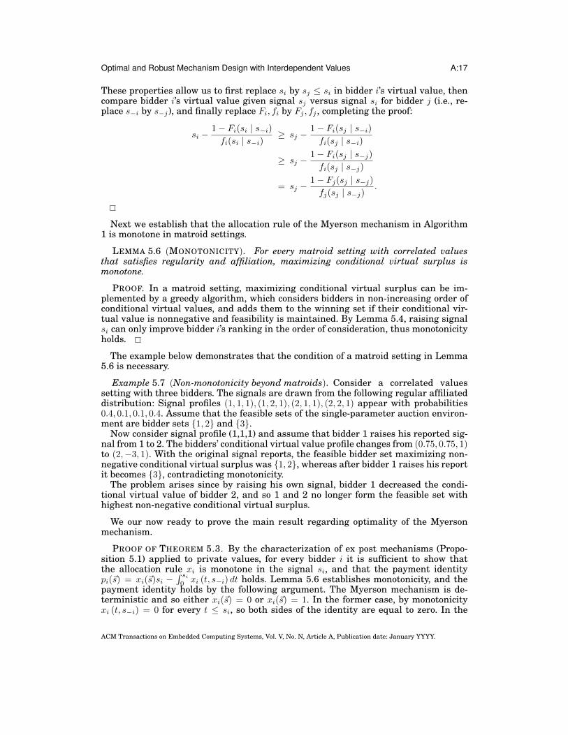
These properties allow us to first replace si by sj ≤ si in bidder i’s virtual value, thencompare bidder i’s virtual value given signal sj versus signal si for bidder j (i.e., re-place s−i by s−j), and finally replace Fi, fi by Fj , fj , completing the proof:

si −1− Fi(si | s−i)fi(si | s−i)

≥ sj −1− Fi(sj | s−i)fi(sj | s−i)

≥ sj −1− Fi(sj | s−j)fi(sj | s−j)

= sj −1− Fj(sj | s−j)fj(sj | s−j)

.

Next we establish that the allocation rule of the Myerson mechanism in Algorithm1 is monotone in matroid settings.

LEMMA 5.6 (MONOTONICITY). For every matroid setting with correlated valuesthat satisfies regularity and affiliation, maximizing conditional virtual surplus ismonotone.

PROOF. In a matroid setting, maximizing conditional virtual surplus can be im-plemented by a greedy algorithm, which considers bidders in non-increasing order ofconditional virtual values, and adds them to the winning set if their conditional vir-tual value is nonnegative and feasibility is maintained. By Lemma 5.4, raising signalsi can only improve bidder i’s ranking in the order of consideration, thus monotonicityholds.

The example below demonstrates that the condition of a matroid setting in Lemma5.6 is necessary.

Example 5.7 (Non-monotonicity beyond matroids). Consider a correlated valuessetting with three bidders. The signals are drawn from the following regular affiliateddistribution: Signal profiles (1, 1, 1), (1, 2, 1), (2, 1, 1), (2, 2, 1) appear with probabilities0.4, 0.1, 0.1, 0.4. Assume that the feasible sets of the single-parameter auction environ-ment are bidder sets {1, 2} and {3}.

Now consider signal profile (1,1,1) and assume that bidder 1 raises his reported sig-nal from 1 to 2. The bidders’ conditional virtual value profile changes from (0.75, 0.75, 1)to (2,−3, 1). With the original signal reports, the feasible bidder set maximizing non-negative conditional virtual surplus was {1, 2}, whereas after bidder 1 raises his reportit becomes {3}, contradicting monotonicity.

The problem arises since by raising his own signal, bidder 1 decreased the condi-tional virtual value of bidder 2, and so 1 and 2 no longer form the feasible set withhighest non-negative conditional virtual surplus.

We our now ready to prove the main result regarding optimality of the Myersonmechanism.

PROOF OF THEOREM 5.3. By the characterization of ex post mechanisms (Propo-sition 5.1) applied to private values, for every bidder i it is sufficient to show thatthe allocation rule xi is monotone in the signal si, and that the payment identitypi(~s) = xi(~s)si −

∫ si0xi (t, s−i) dt holds. Lemma 5.6 establishes monotonicity, and the

payment identity holds by the following argument. The Myerson mechanism is de-terministic and so either xi(~s) = 0 or xi(~s) = 1. In the former case, by monotonicityxi (t, s−i) = 0 for every t ≤ si, so both sides of the identity are equal to zero. In the



latter case, since s∗i is bidder i’s threshold signal, the right-hand side is

si −∫ si

0

xi (t, s−i) dt = si − (si − s∗i ) = s∗i ,

and for private values s∗i is precisely the payment pi(~s) charged by the Myerson mech-anism.

It is left to show optimality. The expected revenue of an ex post IC and ex post IRmechanism is its expected virtual surplus (Proposition 5.2), and the Myerson mecha-nism maximizes virtual surplus for every signal profile.

5.3. Optimal Mechanism for Interdependent ValuesThe results for correlated values generalize to interdependent values, however thissetting is harder and requires further assumptions. Indeed, recall that the generalconditional virtual value form in Equation 1 includes two extra dependencies on otherbidders’ signals relative to the form in Equation 2 which applies to correlated values.The extra assumptions are needed to establish monotonicity of the allocation rule inAlgorithm 1 despite these dependencies.

We adopt the setting studied by Lopomo [2000] in the context of the English auc-tion; namely, the assumptions we impose on our auction setting are that bidders aresymmetric and have affiliated signals (Sections 2.4.3 and 2.4.4), and that the followingconditions on the valuation function and distribution hold.

Definition 5.8 (Lopomo assumptions).

(1) MHR setting (Section 2.4.2);(2) Bidders with higher signals have higher values, i.e., strong single crossing of values

(Section 2.4.5);(3) Bidders with higher signals have lower sensitivity of their value to their signal,

i.e., the partial derivative of vi with respect to si is weakly decreasing in si, andweakly increasing in sj for every other j.

For every signal profile ~s such that si ≥ sj , the Lopomo assumptions imply:

vi(~s) ≥ vj(~s);

d

dsivi(~s) ≤

d

dsjvj(~s). (8)

An example of a symmetric affiliated setting where the Lopomo assumptions holdis a single-item setting with weighted-sum values (Example 2.1), and signals drawnfrom the multivariate normal distribution of Example 2.3. Note that Equation (8) holdswhenever values are multilinear.7

We can now state this section’s main result - an analogue of Theorem 5.3 for in-terdependent values, showing that the Myerson mechanism defined in Algorithm 1 isoptimal.

THEOREM 5.9 (MYERSON MECHANISM IS EX POST IC, IR AND OPTIMAL). For ev-ery symmetric matroid setting with interdependent values that satisfies affiliation andthe Lopomo assumptions, the Myerson mechanism is ex post IC, ex post IR, and optimalamong all ex post IC and ex post IR mechanisms.

7Recall that a function is multilinear if it is separately linear in each one of its variables – weighted sumsand products are examples.



The proof of Theorem 5.9, like the proof of its analogue Theorem 5.3, boils down toshowing monotonicity of the Myerson mechanism. We now turn to establishing mono-tonicity, using that the the order of conditional virtual values coincides with the or-der of signals. This strong form of single crossing for conditional virtual values (cf.,Lemmas 5.4 and 5.5) is stated in the following lemma, which can be viewed as a gen-eralization of the same result in the IPV model for a symmetric setting that satisfiesregularity.

LEMMA 5.10 (ORDER OF VIRTUAL VALUES MATCHES ORDER OF SIGNALS). Forevery symmetric setting with interdependent values that satisfies affiliation and theLopomo assumptions, for every signal profile ~s such that si ≥ sj , the bidder with highersignal has higher conditional virtual value

ϕi(si | s−i) ≥ ϕj(sj | s−j).

PROOF. Given a signal profile ~s where si ≥ sj , we show that ϕi(si | s−i) ≥ ϕj(sj |s−j). Recall

ϕi(si | s−i) = v(si, s−i)−1− Fi(si | s−i)fi(si | s−i)

· ddsi

v(si, s−i);

ϕj(sj | s−j) = v(sj , s−j)−1− Fj(sj | s−j)fj(sj | s−j)

· d

dsjv(sj , s−j).

We now compare the right-hand-side terms of the above equations.By the second Lopomo assumption, bidders with higher signals have higher val-

ues and so v(si, s−i) ≥ v(sj , s−j). By the third Lopomo assumption, bidders withhigher signals have a lower sensitivity of their value to their own signal and so0 ≤ d

dsiv(si, s−i) ≤ d

dsjv(sj , s−j) (using the assumption that values are increasing in

signals).It is left to show that 0 ≤ 1−Fi(si|s−i)

fi(si|s−i)≤ 1−Fj(sj |s−j)

fj(sj |s−j). The following three inequali-

ties follow from the first Lopomo assumption of MHR, the affiliation assumption andresulting hazard rate dominance [Krishna 2010, Appendix D], and the bidders’ sym-metry and symmetry of distributions, respectively. These properties allow us to firstreplace si by sj ≤ si in bidder i’s inverse hazard rate, then compare the hazard ratesgiven signal sj versus signal si for bidder j (i.e., replace s−i by s−j), and finally replaceFi, fi by Fj , fj to complete the proof:

1− Fi(si | s−i)fi(si | s−i)

≤ 1− Fi(sj | s−i)fi(sj | s−i)

≤ 1− Fi(sj | s−j)fi(sj | s−j)

=1− Fj(sj | s−j)fj(sj | s−j)

.

We remark that in addition to the set of conditions in the statement of Lemma 5.10,there are also different (incomparable) conditions that suffice to prove a form of singlecrossing for conditional virtual values. One example of an alternative set of sufficientconditions excluding bidder symmetry is affiliated signals and the Lopomo assump-



tions, where we strengthen the first Lopomo assumption to the generalized MHR as-sumption of Li [2013].8

Lemma 5.10 implies that the Myerson mechanism is monotone.

LEMMA 5.11 (MONOTONICITY). For every symmetric matroid setting with inter-dependent values that satisfies affiliation and the Lopomo assumptions, maximizingconditional virtual surplus is monotone.

PROOF. By Lemma 5.10, raising signal si only improves bidder i’s ranking in thegreedy order of consideration by conditional virtual value. This is sufficient for mono-tonicity by a similar argument to that in the proof of Lemma 5.6.

Monotonicity is sufficient to now prove optimality of the Myerson mechanism.

PROOF OF THEOREM 5.9. By the characterization of ex post mechanisms (Proposi-tion 5.1) applied to interdependent values, for every bidder i it is sufficient to showthat the allocation rule xi is monotone in the signal si, and that the payment identityand payment inequality hold. Lemma 5.11 establishes monotonicity. The payment in-equality pi(0, s−i) ≤ xi(0, s−i)vi(0, s−i) holds with equality since if xi(0, s−i) = 0 thenpi(0, s−i) = 0, and if xi(0, s−i) = 1 then pi(0, s−i) = vi(s

∗i , s−i) where s∗i = 0. As for the

payment identity, by determinism and monotonicity of the Myerson mechanism andassuming xi(~s) = 1,

xi(~s)vi(~s)−∫ vi(si,s−i)

vi(0,s−i)

xi(v−1i (t | s−i), s−i

)dt = vi(~s)− (vi(si, s−i)− vi(s∗i , s−i))

= vi(s∗i , s−i)

= pi(~s)

It is left to show optimality. By Proposition 5.2, the expected revenue of an ex postIC and ex post IR mechanism is equal to its expected virtual surplus up to an additiveterm Es−i [

∑i (xi(0, s−i)vi(0, s−i)− pi(0, s−i))]. The Myerson mechanism maximizes the

virtual surplus for every signal profile, and sets the non-negative additive term to zero,thus achieving optimality.

5.4. Indirect Implementation via English AuctionFor completeness, we conclude this section with results by Lopomo [2000] and Chungand Ely [2007] on implementing the optimal mechanism via the English auction witha carefully chosen reserve, when there’s a single item for sale and the bidders are sym-metric. The relation between the previous subsections and these results is the sameas the relation between Myerson’s original mechanism and the following well-knownresult in the IPV model – the second-price auction with an optimal reserve maximizesthe expected revenue from selling a single item when bidders are symmetric and reg-ularity holds. By replacing the second-price auction with the English auction, and set-ting the reserve price after all bidders but one have dropped out and revealed theirinformation, we get an indirect implementation of the optimal mechanism that worksdirectly in value space.

COROLLARY 5.12 ([CHUNG AND ELY 2007]). For every symmetric single-item set-ting with correlated values that satisfies regularity and affiliation, the English auctionwith optimal reserve price is optimal among all ex post IC and ex post IR mechanisms.

8The generalized MHR condition defined and utilized in [Li 2013] states that the second term in Equation1 is decreasing in si for all i and s−i.



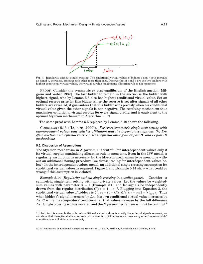
Fig. 1. Regularity without single crossing. The conditional virtual values of bidders i and j both increaseas signal si increases, crossing each other more than once. Observe that if i and j are the two bidders withhighest conditional virtual values, the virtual-surplus-maximizing allocation rule is not monotone.

PROOF. Consider the symmetric ex post equilibrium of the English auction [Mil-grom and Weber 1982]. The last bidder to remain in the auction is the bidder withhighest signal, who by Lemma 5.5 also has highest conditional virtual value. Set anoptimal reserve price for this bidder. Since the reserve is set after signals of all otherbidders are revealed, it guarantees that this bidder wins precisly when his conditionalvirtual value given the other signals is non-negative. The resulting mechanism thusmaximizes conditional virtual surplus for every signal profile, and is equivalent to theoptimal Myerson mechanism in Algorithm 1.

The same proof with Lemma 5.5 replaced by Lemma 5.10 shows the following.

COROLLARY 5.13 ([LOPOMO 2000]). For every symmetric single-item setting withinterdependent values that satisfies affiliation and the Lopomo assumptions, the En-glish auction with optimal reserve price is optimal among all ex post IC and ex post IRmechanisms.

5.5. Discussion of AssumptionsThe Myerson mechanism in Algorithm 1 is truthful for interdependent values only ifits virtual-surplus-maximizing allocation rule is monotone. Even in the IPV model, aregularity assumption is necessary for the Myerson mechanism to be monotone with-out an additional ironing procedure (we dicuss ironing for interdependent values be-low). In the interdependent values model, an additional single crossing assumption forconditional virtual values is required. Figure 1 and Example 5.14 show what could gowrong if this assumption is violated.

Example 5.14 (Regularity without single crossing in a wallet game). Consider asymmetric, single-item setting with non-private values. Let the values be weighted-sum values with parameter β = 1 (Example 2.1), and let signals be independentlydrawn from the regular distribution G(s) = 1 − s−2. Plugging into Equation 3, theconditional virtual value of bidder i is

∑j sj − (1−G(si))/g(si) = si/2 +

∑j 6=i sj . Thus

when bidder i’s signal increases by ∆si, his own conditional virtual value increases by∆si/2 while his competitors’ conditional virtual values increase by the full difference∆si. Single crossing is thus violated and the Myerson mechanism will not be truthful.9

9In fact, in this example the order of conditional virtual values is exactly the order of signals reversed; wecan show that the optimal allocation rule in this case is to pick a random winner – any other “more sensible”allocation rule will violate monotonicity.



Single crossing as an assumption in itself is quite opaque; above we have identifiedeconomically-meaningful conditions on the auction environment that are sufficient forsingle crossing to hold, both in the special case of correlated values and in the moregeneral case of interdependent values. While the standard assumption of affiliation issufficient in the correlated values setting, this is no longer the case for full interdepen-dence. However, as we have seen, symmetry together with the Lopomo assumptionsare sufficient (and alternative sufficient conditions exist as well). While the knowncomputational hardness results imply that some of these assumptions (or alternativeones) are required for optimality of the deterministic Myerson mechanism, achievinga precise understanding of what is necessary remains an open question.

Ironing. Does the method of ironing developed by Myerson [1981] work for interde-pendent values?10 Technically, the ironing method can easily be applied to conditionalvirtual values, i.e., the Myerson mechanism with ironing is well-defined for interde-pendent values. Furthermore, it still holds that ironed conditional virtual surplus givesan upper bound on conditional virtual surplus, which is tight for mechanisms that “re-spect” the ironed intervals (in the sense that the allocation does not change along suchan interval).

The crucial difference from the IPV model is that the expected revenue of the Myer-son mechanism with ironing can be strictly lower than the expected ironed conditionalvirtual surplus. Thus, even though the Myerson mechanism with ironing truthfullymaximizes the latter, it is no longer guaranteed to achieve the maximum expected rev-enue. This gap arises due to the fact that the Myerson mechanism with ironing doesnot respect ironed intervals. Indeed, while the increase in a bidder’s signal does notchange his ironed conditional virtual value within an ironed segment, it may changeothers’ ironed conditional virtual values, thus modifying the allocation.

Since the Myerson mechanism with ironing is deterministic, it is not surprising thatironing does not allow us to dispose altogether of assumptions on the valuations and/ordistributions, as is the case in Myerson’s paper (recall the negative results in [Dobzin-ski et al. 2011; Papadimitriou and Pierrakos 2011]). It is open whether ironing canhelp weaken these assumptions.

6. PRIOR-INDEPENDENCE FOR NON-PRIVATE VALUESIn this section we begin to develop a theory of prior-independence for interdependentvalues. Our main result is, for non-private values and the setting studied above (Sec-tion 5.3), a prior-independent mechanism that achieves a constant-factor approxima-tion to the optimal expected revenue. An interesting direction for future work is todesign good prior-independent mechanisms for general interdependent values.

This section is organized as follows: After presenting the setting and stating themain result, we prove our result for a simple single item setting in which biddersshare a pure common value for the item. Section 6.5 generalizes the proof to matroidsettings with non-private values.

6.1. SettingWe study a matroid setting with non-private values where signals are independent,and the Lopomo assumptions (Definition 5.8) hold.11

10A description of the ironing method is beyond the scope of this paper; for an introduction see, e.g., [Hartline2012].11Note that for digital goods settings, our results hold more generally; i.e., we no longer need all the Lopomoassumptions.



ALGORITHM 2: The Single Sample Mechanism for Interdependent Values(1) Elicit signal reports ~s from the bidders.(2) Choose a reserve bidder uniformly at random, denote his signal by sr.(3) Place the feasible set of non-reserve bidders with highest signals in a “potential winners”

set P . Break ties arbitrarily but consistently.(4) Allocate to every bidder i ∈ P such that si ≥ sr.(5) Charge every winner i a payment vi(max{sr, ti}, s−i), where ti is the threshold signal below

which, given the signals of the other non-reserve bidders, i would not belong to P .

Symmetry. As is standard in the prior-independence literature (see, e.g., [Bulow andKlemperer 1996; Goldberg et al. 2006; Segal 2003; Dhangwatnotai et al. 2010]), wefocus on symmetric environments with n ≥ 2 bidders.

Notation. As above, let F denote the joint distribution of the independent signals.Let G be the distribution from which each of the i.i.d. signals is drawn, and let g bethe corresponding density (G is the marginal distribution of the signals given the jointproduct distribution F ). We denote by G|s−i

(·), g|s−i(·) the distribution and density of

bidder i’s value given the signal profile s−i of the other bidders.

Remark 6.1 (Strong MHR guarantee). Observe that by independence, G|s−i(·) is

simply the distribution of si. It follows that the inverse hazard rate of bidder i’s valuegiven signal profile ~s is

1−G|s−i(vi(~s))

g|s−i(vi(~s))

=1−G(si)

g(si)· ddsi

vi(~s). (9)

By the first and third Lopomo assumptions, the inverse hazard rate in Equation 9 isweakly decreasing in si. We conclude that not only the signal distribution G is MHR,but also, for every bidder i, so is the value distribution G|s−i

for every signal profiles−i.

6.2. The Single Sample Mechanism for Interdependent ValuesWe describe our prior-independent mechanism for interdependent values in Algorithm2. It is a natural generalization of the single sample mechanism of Dhangwatnotaiet al. [2010]. Observe that the mechanism makes no reference to the distribution G.12

We are now ready to state this section’s main result – that the above prior-independent mechanism is near-optimal. We compare its expected revenue to OPT,the optimal expected revenue achieved by the generalization of Myerson’s mechanismto interdependent values (Algorithm 1). In fact, due to the MHR setting, the proof willbe able to relate the expected revenue to the expected welfare, establishing a stongerproperty of effectiveness as defined by Neeman [2003].

THEOREM 6.2 (SINGLE SAMPLE IS NEAR-OPTIMAL). Let n ≥ 2 and consider asymmetric matroid setting with non-private values in which the Lopomo assumptionshold. The prior-independent single sample mechanism in Algorithm 2 yields a constantfactor approximation to OPT.

12We remark that the mechanism is assumed to know the valuation function vi. An intriguing open problemis to design a mechanism, perhaps based on an ascending or multi-stage auction, for which this assumptioncan be dropped.



6.3. Useful Properties of MHR DistributionsWe motivate our focus on MHR settings by the following example, which shows thatunlike independent private values for which regularity suffices, for interdependentvalues a stronger MHR assumption is necessary to guarantee near-optimality of thesingle sample mechanism. Note that unlike previous sections, the MHR assumptionis for the approximation guarantee (weaker assumptions are sufficient for incentivesonly). More generally, the example demonstrates how interdependence can pose newtechnical challenges, arising from the information externalities among bidders. Theoriginal analysis of Dhangwatnotai et al. [2010] no longer applies; we present proper-ties of MHR distributions that will be useful in the new analysis.

Example 6.3 (Non-MHR setting). Consider a digital goods setting with two bid-ders, whose i.i.d. signals are drawn from the equal revenue distribution G(s) =1 − (1/s), truncated to a finite range [1, H], where H is an arbitrarily large constant.The bidders have weighted-sum values with β = 1, i.e., their pure common value iss1 + s2 (see Example 2.1). The optimal expected revenue in this setting is at leastE[s1] + E[s2] ≈ 2 lnH, by charging each bidder the signal of the other. However, theexpected revenue of the single sample mechanism is 2E[min{s1, s2}], which is� H.

The gap in Example 6.3 between the expectation of the distribution and the expec-tation of the lower among two random samples is due to the long tail of the non-MHRequal revenue distribution; we now show that for MHR distributions this issue doesnot arise. The next lemma is tight for the exponential distribution.

LEMMA 6.4 (LOWER AMONG TWO SAMPLES FROM MHR DISTRIBUTION). Let s, s′be two i.i.d. samples drawn from an MHR distribution, then

E[s | s ≤ s′] ≥ 1

2E[s].

PROOF. Let G with density g be the MHR distribution. Let h(·) be the hazard ratefunction of G and let H(·) be its cumulative hazard rate, i.e., h(s) = g(s)/(1 − G(s)),and H(s) =

∫ s0h(z)dz. By definition of the hazard rate function, 1−G(s) = exp(−H(s)).

Since G is MHR, h(·) is non-negative and weakly increasing, therefore H(·) is weaklyincreasing and convex. We can now write

E[s | s ≤ s′] =

∫ ∞0

e−2H(s) ≥∫ ∞0

e−H(2s) ≥ 1

2

∫ ∞0

e−H(s) =1

2E[s],

where the first equality is by plugging in the distribution of the lower among twosamples into E[x] =

∫∞0

1− F (z)dz, the first inequality is by convexity of H, and thesecond inequality is via integration by substitution.

We now state a version of the previous lemma with an added threshold (and a nec-essarily slightly increased constant).

LEMMA 6.5 (LOWER AMONG TWO SAMPLES WITH THRESHOLD). Let s, s′ be twoi.i.d. samples drawn from an MHR distribution. For every threshold t ≥ 0,

E[max{s, t} | max{s, t} ≤ s′] ≥ 1

3E[s | s ≥ t].

PROOF. Recall we’d like to show that

E[max{s, t} | max{s, t} ≤ s′] ≥ 1

3E[s | s ≥ t],



where s, s′ are i.i.d. samples from an MHR distribution and t is a threshold. Since s isdrawn from an MHR distribution we can write

1

3(t+ E[s]) ≥ 1

3E[s | s ≥ t].

Assume first that t ≤ E[s]/2, then

E[max{s, t} | max{s, t} ≤ s′] ≥ E[s | s ≤ s′] ≥ E[s]/2 ≥ 1

3(t+ E[s]),

where the second inequality is by Lemma 6.4 and the last one is by assumption. Wenow turn to the case in which t > E[s]/2, and complete the proof by observing that

E[max{s, t} | max{s, t} ≤ s′] ≥ t ≥ 1

3(t+ E[s]).

The following simple lemmas are stated without proofs.

LEMMA 6.6 (CONDITIONAL MHR DISTRIBUTION). Let signal s be randomlydrawn from an MHR distribution. For any threshold t, the distribution of s conditionalon s ≥ t is also MHR.

LEMMA 6.7 (OPTIMAL REVENUE APPROXIMATES WELFARE [HARTLINE 2012]).In a single bidder setting where the bidder’s value is drawn from an MHR distribution,the optimal expected revenue is at least a 1/e fraction of the expected value.

LEMMA 6.8 (MEDIAN AS RESERVE FOR REGULAR DISTRIBUTIONS [AZAR ET AL. 2013]).In a single bidder setting where the bidder’s value is drawn from a regular distributionG, a reserve price equal to the median of G guarantees at least half the optimal expectedrevenue, and the optimal expected revenue is thus at most the median.

6.4. Proof for Simple Setting: Single Item with Common ValueIn this section we prove Theorem 6.2 for a simple setting with a single item for sale,which is valued the same by all bidders. We first state and prove our main lemma.

Main lemma. Let s1, s2 be i.i.d. signals drawn from an MHR distribution G. Con-sider a single bidder with value v(s1, s2), where v is a symmetric valuation functionincreasing in its arguments. Fixing signal s1 (resp., s2), let the value distribution G|s1(resp., G|s2 ) be an MHR distribution. Let c = 1/8e (where e is the base of the naturallogarithm).13

LEMMA 6.9 (REUSING SAMPLE APPROXIMATES WELFARE).Es1,s2 [v(s2, s2) | s2 ≤ s1] ≥ cEs1,s2 [v(s1, s2)]. (10)

In words, plugging in the lower among s1, s2 into the valuation function decreases theexpected value by a factor of no more than c.

PROOF. Let m be the median of distribution G. We begin with the left-hand side ofEquation 10 and condition on the event that s2 ≥ m, which given that s2 ≤ s1 occurswith probability 1/4. Using that v is non-decreasing,

Es1,s2 [v(s2, s2)|s2 ≤ s1] ≥ Prs1,s2

[s2 ≥ m | s2 ≤ s1]Es1,s2 [v(s2, s2) | m ≤ s2 ≤ s1]

≥ 1

4Es1,s2 [v(m, s2) | s2 ≤ s1].

13We do not optimize the constant c.



Now we know that replacing a random MHR sample with the lower among two sam-ples results in a loss of at most 1/2 (Lemma 6.4). This can be applied to the distributionG|s1=m of v(m, ·), which is MHR by assumption. We get that

Es1,s2 [v(m, s2) | s2 ≤ s1] ≥ 1

2Es2 [v(m, s2)].

Now fix s2. Observe that by the signal independence assumption, v(m, s2) is the medianof the MHR distribution G|s2 of v(·, s2). Thus

v(m, s2) ≥ 1

eEs1 [v(s1, s2)],

where the inequality follows by combining Lemma 6.8, by which the median upperbounds the optimal expected revenue, with Lemma 6.7, by which the optimal ex-pected revenue and expected welfare are close. Taking expectation over s2 completesthe proof.

We are now ready to prove the special case of our main theorem – near-optimality ofthe single sample mechanism for the simple single-item, common value setting.

PROOF OF THEOREM 6.2 FOR SINGLE ITEM WITH COMMON VALUE. Let v(~s) be thepure common value of the item for the bidders, whose i.i.d. signals s1, . . . , sn are drawnfrom an MHR distribution G. In this simple setting, the single sample mechanism inAlgorithm 2 reduces to the following mechanism: choose a random reserve bidder; withprobability (n − 1)/n the bidder with highest signal is not chosen as reserve; he thenwins the item and is charged according to the second highest signal. We claim that inexpectation, the revenue achieved by this VCG-like mechanism is a c(n− 1)/n-fractionof the expected welfare E~s[v(s1, . . . , sn)], where c is as above.

The proof is by reduction to the single bidder setting of Lemma 6.9 (where the singlebidder will correspond to the highest bidder). From now on we condition on the highestbidder not being chosen as reserve, incurring a loss of (n− 1)/n.

Fix the n − 2 lowest signals, denoted without loss of generality s3 ≥ · · · ≥ sn. Letv(·, ·) = v(·, ·, s3, . . . , sn) be the valuation function given the fixed signals. Let G be thedistribution G conditioned on exceeding the threshold s3. By Lemma 6.6, G is MHR,and the two highest signals s1, s2 can be seen as i.i.d. random draws from G. One ofthese is the second highest signal, and so we can write the expected revenue of thesingle sample mechanism as

Es1,s2∼G[v(s2, s2) | s2 ≤ s1]. (11)

In order to apply the main lemma (Lemma 6.9) to lower bound the expected revenuein 11, recall that v and hence v are symmetric and increasing. It is left to show thatG|s1and G|s2 are MHR. Without loss of generality consider G|s2 . We know from Remark 6.1that given s2, . . . , sn, the distribution of v|s−1

is MHR. If we condition this distributionon v|s−1

being at least as high as v|s−1(s3), we still get an MHR distribution by Lemma

6.6. The resulting distribution is precisely the distribution G|s2 .The proof can now be completed by applying Lemma 6.9 to get that the expected

revenue in (11) is at least cEs1,s2∼G[v(s1, s2)] for any fixed profile s3, . . . , sn, and finallyby taking expectation over s3, . . . , sn according to the joint distribution of the n − 2lowest among n draws from G.



6.5. Proof for General SettingIn this section we prove Theorem 6.2 for a general matroid setting in which biddershave symmetric but distinct values. The proof relies on an extension of the main lemma(Lemma 6.9) above.

As above, let s1, s2 be i.i.d. signals drawn from an MHR distribution G. Considera single bidder with a symmetric and increasing valuation v(s1, s2), and assume thevalue distributions G|s1 and G|s2 when one of the signals is fixed are MHR. Let c′ =

1/12e.14

LEMMA 6.10 (REUSING SAMPLE WITH THRESHOLD). For every threshold t ≥ 0,

Es1,s2 [v(max{s2, t}, s2) | max{s2, t} ≤ s1] ≥ c′Es1,s2 [v(s1, s2) | t ≤ s1].

PROOF. Recall we want to show that, for c′ = 1/12e,

Es1,s2 [v(max{s2, t}, s2) | max{s2, t} ≤ s1] ≥ c′Es1,s2 [v(s1, s2) | t ≤ s1].

Let m be the median of distribution G from which s1, s2 are independently drawn.Similarly to the proof of Lemma 6.9 we have that

Es1,s2 [v(max{s2, t}, s2) | max{s2, t} ≤ s1] ≥ 1

4Es1,s2 [v(max{s2, t},m) | max{s2, t} ≤ s1].

By Lemma 6.5 applied to the distribution G|s2=m of v(·,m), which is MHR by assump-tion, and using that v is weakly increasing, we get

1

4Es1,s2 [v(max{s2, t},m) | max{s2, t} ≤ s1] =

1

4Es1,s2 [max{v(s2,m), v(t,m)} | max{v(s2,m), v(t,m)} ≤ v(s1,m)] ≥

1

12Es1 [v(s1,m) | s1 ≥ t].

Similarly to the proof of Lemma 6.9, we now fix s1 ≥ t. Observe that v(s1,m) is themedian of the MHR distribution G|s1 of v(s1, ·). Thus

v(s1,m) ≥ 1

eEs2 [v(s1, s2)],

and taking expectation over s1 conditional on s1 ≥ t completes the proof.

The proof of Theorem 6.2 for the general setting is by reduction to the single biddersetting and application of Lemma 6.10.

PROOF OF THEOREM 6.2 FOR GENERAL SETTING. Recall we wish to analyze theexpected revenue of the single sample mechanism in Algorithm 2, for a symmetricmatroid setting with n ≥ 2 bidders, where the i.i.d. signals s1, . . . , sn are drawn froman MHR distribution G. Denote by v the symmetric valuation function of the bidders.Similarly to the proof in Section 6.4, we will reduce this setting to a single biddersetting to which Lemma 6.10 is applicable.

Without loss of generality we name the chosen reserve bidder “bidder 2”, and con-sider an arbitrary non-reserve bidder “bidder 1”. We condition on the signals of allbidders other than 1 and 2 and omit them from the notation, i.e., we use the notationv(s1, s2) for bidder 1’s value. In addition, we denote by t the threshold for bidder 1 to

14As before, the constant is not optimized.



belong in the potential winner set P given the fixed signals. We can now write the ex-pected contribution of bidder 1 to the expected revenue of the single sample mechanismas

Es1,s2 [v(max{s2, t}, s2) | max{s2, t} ≤ s1] Pr[max{s2, t} ≤ s1]. (12)

In what follows we show that the expected contribution in 12 is a constant fractionof the expected contribution of bidder 1 to the expected maximum welfare excludingbidder 2. To see how this completes the proof, take expectation over the fixed signalsand sum up over non-reserve bidders. The total expected revenue of the single samplemechanism is thus a constant fraction of the welfare excluding the reserve bidder,which is in turn a (n− 1)/n fraction of the total welfare.

We begin by writing down the expected contribution of bidder 1 to the expected maxi-mum welfare excluding bidder 2. Crucially, the same threshold t as in the single samplemechanism is the threshold for bidder 1 to be included in the welfare-maximizing setof bidders. This is because the potential winner set P of the single sample mechanismis the feasible set of non-reserve bidders with highest signals, and by single-crossing ofvalues (second Lopomo assumption) and the matroid setting, this is also the welfare-maximizing feasible set. The expected welfare contribution is thus

Es1,s2 [v(s1, s2) | s1 ≥ t] Pr[s1 ≥ t]. (13)

It remains to compare (12) to (13). Since we know that v is symmetric and increasingand that v(s1, ·), v(·, s2) are distributed according to an MHR distribution (Remark 6.1),we can apply Lemma 6.10 to get

Es1,s2 [v(max{s2, t}, s2) | max{s2, t} ≤ s1] Pr[max{s2, t} ≤ s1] ≥c′Es1,s2 [v(s1, s2) | s1 ≥ t] Pr[s1 ≥ t] Pr[s1 ≥ s2 | s1 ≥ t] ≥

c′Es1,s2 [v(s1, s2) | s1 ≥ t] Pr[s1 ≥ t] Pr[s1 ≥ s2] =

(c′/2)Es1,s2 [v(s1, s2) | s1 ≥ t] Pr[s1 ≥ t].

7. OPEN QUESTIONSInterdependent values are potentially a new frontier for algorithmic mechanism de-sign; we conclude with a non-exhaustive list of directions for further research.

(1) Ex post optimal and near-optimal mechanism design:(a) Optimality: For correlated values, in the absence of regularity and single cross-

ing, finding the optimal mechanism may be a computationally hard problem.Are there weaker conditions (e.g., just single crossing but not regularity) underwhich a meaningful description of the optimal mechanism is available, perhapsvia some form of Myerson-inspired ironing (cf., [Myerson 1981])? Is random-ness necessary to achieve optimality (cf., irregular non-single crossing examplerequiring randomness in [Dobzinski et al. 2011])? Similar questions apply tointerdependent values, where the goal would also be to weaken the Lopomo as-sumptions. Identifying tractable settings for the optimal mechanism problemmay also have direct applicability to the efficient mechanism problem.

(b) Approximation: For correlated values, Dobzinski et al. [2011] show a near-optimal mechanism that does not rely on regularity or affiliation assumptions.Their mechanism is based on the appealing lookahead mechanism of Ronen[2001]. Is there a parallel result for interdependent values?

(c) Simple, natural and practical mechanisms (as advocated in [Hartline andRoughgarden 2009]). For example, when the English auction is not optimal,



under what conditions is it approximately-optimal? See Li [2013] for one set ofsufficient conditions.

(2) Beyond ex post mechanisms: There is a range of robustness levels to explore inmechanism design, and it is far from clear what is the “right” level. This may de-pend on information asymmetries in the market (e.g., is it reasonable/necessaryto assume public knowledge of valuation functions), as well as on models of play-ers’ risk-averseness and on practical considerations, such as the difficulty to collectpayments from losing bidders (e.g., this motivates the “losers do not pay” conditionconsidered by Lopomo [2000]). What are the most economically-meaningful robust-ness requirements, and what are optimal and approximately-optimal mechanismsthat achieve them?

(3) Beyond optimal mechanism design: Interdependent values are an active researcharea in the design of other economic mechanisms and markets, to which computa-tional insight potentially has much to contribute – see for example Satterthwaiteet al. [2011] on double auctions, Che and Kim [2012] on house allocation or Csapoand Muller [2013] on public goods.

ACKNOWLEDGMENTS

The authors wish to thank Moshe Babaioff, Paul Milgrom, Uri Nadav and the anonymous reviewers forhelpful comments, as well as participants of the Market Design course at Stanford, the EconCS seminar atHarvard and the Theory seminar at Northwestern. In an earlier version of this work we presented Corollary5.12 unaware that it appeared in a paper of Chung and Ely [2007]; we are grateful to Gabriel Carroll forpointing us to their paper.

REFERENCESALON, N. AND SPENCER, J. H. 2008. The Probabilistic Method. Wiley.AZAR, P., DASKALAKIS, C., MICALI, S., AND WEINBERG, S. M. 2013. Optimal and efficient parametric

auctions. In SODA13. 596–604.BERGEMANN, D. AND MORRIS, S. 2005. Robust mechanism design. Econometrica 73, 6, 1771–1813.BIKHCHANDANI, S., HAILE, P. A., AND RILEY, J. G. 2002. Symmetric separating equilibria in English

auctions. Games and Economic Behavior 38, 19–27.BRANCO, F. 1996. Multiple unit auctions of an indivisible good. Economic Theory 8, 77–101.BULOW, J. AND KLEMPERER, P. 1996. Auctions versus negotiations. American Economic Review 86, 1, 180–

194.CAI, Y., DASKALAKIS, C., AND WEINBERG, M. 2012. Optimal multi-dimensional mechanism design: Reduc-

ing revenue to welfare maximization. In Proc. 53rd IEEE Symp. on Foundations of Computer Science(FOCS). 130–139.

CHE, Y.-K. AND KIM, J. 2012. Efficient assignment with interdependent values. Working paper.CHEN, X., HU, G., LU, P., AND WANG, L. 2011. On the approximation ratio of k-lookahead auction. In

Workshop on Internet and Network Economics (WINE). 61–71.CHUNG, K. AND ELY, J. C. 2006. Ex-post incentive compatible mechanism design. Manuscript.CHUNG, K.-S. AND ELY, J. C. 2007. Foundations of dominant-strategy mechanisms. The Review of Economic

Studies 74, 2, 447–476.COMPTE, O. AND JEHIEL, P. 2009. Veto constraint in mechanism design: Inefficiency with correlated types.

American Economic Journal: Microeconomics 1, 1, 182–206.CREMER, J. AND MCLEAN, R. P. 1985. Optimal selling strategies under uncertainty for a discriminating

monopolist when demands are interdependent. Econometrica 53, 2, 345–361.CREMER, J. AND MCLEAN, R. P. 1988. Full extraction of the surplus in bayesian and dominant strategy

auctions. Econometrica 56, 6, 1247–1257.CSAPO, G. AND MULLER, R. 2013. Optimal mechanism design for the private supply of a public good. To

appear in Games and Economic Behavior.DE CASTRO, L. I. 2010. Affiliation, equilibrium existence and revenue ranking of auctions. Working Paper.DE CASTRO, L. I. AND PAARSCH, H. J. 2010. Testing affiliation in private-values models of first-price auc-

tions using grid distributions. Annals of Applied Statistics 4, 4, 2073–2098.



DHANGWATNOTAI, P., ROUGHGARDEN, T., AND YAN, Q. 2010. Revenue maximization with a single sample.In Proc. 11th ACM Conf. on Electronic Commerce (EC). 129–138.

DOBZINSKI, S., FU, H., AND KLEINBERG, R. 2011. Optimal auctions with correlated bidders are easy. InProc. 42nd ACM Symp. on Theory of Computing (STOC). 129–138.

GOLDBERG, A. V., HARTLINE, J. D., KARLIN, A., SAKS, M., AND WRIGHT, A. 2006. Competitive auctions.Games and Economic Behavior 55, 2, 242–269.

HARTLINE, J. 2012. Approximation in economic design. Book manuscript.HARTLINE, J. D. AND ROUGHGARDEN, T. 2009. Simple versus optimal mechanisms. In Proc. 10th ACM

Conf. on Electronic Commerce (EC). 225–234.JEHIEL, P., TER VEHN, M. M., MOLDOVANU, B., AND ZAME, W. 2006. The limits of ex-post implementation.

Econometrica 74, 3, 585–610.KLEMPERER, P. 1998. Auctions with almost common values: The “wallet game” and its applications. Euro-

pean Economic Review 42, 3, 757–769.KLEMPERER, P. 1999. Auction theory: A guide to the literature. Journal of Economic Surveys 13, 227–286.KRISHNA, V. 2010. Auction Theory Second Ed. Academic Press.LI, Y. 2013. Approximation in mechanism design with interdependent values. In Proc. 14th ACM Conf. on

Electronic Commerce (EC). 675–676.LOPOMO, G. 2000. Optimality and robustness of the english auction. Games and Economic Behavior 36,

219–240.MCAFEE, R. P. AND RENY, P. J. 1992. Correlated information and mechanism design. Econometrica 60, 2,

395–421.MILGROM, P. 2004. Putting Auction Theory to Work. Cambridge University Press.MILGROM, P. AND WEBER, R. J. 1982. A theory of auctions and competitive bidding. Econometrica 50,

1089–1122.MYERSON, R. 1981. Optimal auction design. Mathematics of Operations Research 6, 1, 58–73.NEEMAN, Z. 2003. The effectiveness of English auctions. Games and Economic Behavior 43, 2, 214–238.NISAN, N. 2007. Introduction to mechanism design (for computer scientists). In Algorithmic Game Theory,

N. Nisan, T. Roughgarden, E. Tardos, and V. Vazirani, Eds. Cambridge University Press, Chapter 9,209–241.

OXLEY, J. G. 1992. Matroid Theory. Oxford.PAPADIMITRIOU, C. AND PIERRAKOS, G. 2011. On optimal single-item auctions. In Proc. 52nd IEEE Symp.

on Foundations of Computer Science (FOCS).RONEN, A. 2001. On approximating optimal auctions. In Proc. 3rd ACM Conf. on Electronic Commerce (EC).

11–17.RONEN, A. AND SABERI, A. 2002. On the hardness of optimal auctions. In Proc. 43rd IEEE Symp. on

Foundations of Computer Science (FOCS). 396–405.SATTERTHWAITE, WILLIAMS, AND ZACHARIADIS. 2011. Price discovery. Working Paper.SEGAL, I. 2003. Optimal pricing mechanisms with unknown demand. American Economic Review 93, 3,

509–529.ULKU, L. 2012. Optimal combinatorial mechanism design. To appear in Economic Theory.VOHRA, R. V. 2011. Mechanism Design: A Linear Programming Approach (Econometric Society Mono-

graphs). Cambridge University Press.WILSON, R. 1987. Game-theoretic analyses of trading processes. Advances in Economic Theory: Fifth World

Congress, 33–70.WILSON, R. B. 1969. Competitive bidding with disparate information. Management Science 15, 7, 446–448.

A. MISSING PROOFS RELATED TO MYERSON THEORY (SECTION 5)PROOF OF PROPOSITION 5.1 (FOLLOWING [NISAN 2007], THEOREM 9.39). We

fix i, s−i and omit them from the notation for simplicity.

First direction. Assume x is monotone and the payment identity and inequality hold.For ex post IC we need to show that x(s)v(s)− p(s) ≥ x(s′)v(s)− p(s′) for every s 6= s′.



Plugging in the payment identity, we need to show∫ v(s)

v(0)

x(v−1(t)

)dt ≥ x(s′) (v(s)− v(s′)) +

∫ v(s′)

v(0)

x(v−1(t)

)dt.

If s′ > s, this is equivalent to x(s′) (v(s′)− v(s)) ≥∫ v(s′)v(s)

x(v−1(t)

)dt, which holds by

monotonicity of x, and if s > s′ a similar argument applies. For ex post IR we need toshow

∫ v(s)v(0)

x(v−1(t)

)dt+x(0)v(0)− p(0) ≥ 0, and this holds since x is non-negative and

x(0)v(0) ≥ p(0).

Second direction. Assume ex post IR. So for every s′ > s, x(s)v(s)−p(s) ≥ x(s′)v(s)−p(s′) and x(s)v(s′) − p(s) ≤ x(s′)v(s′) − p(s′). Subtracting the inequalities we getx(s) (v(s)− v(s′)) ≥ x(s′) (v(s)− v(s′)), which implies monotonicity by the assumptionthat v(·) is strictly increasing in its argument. To derive the payment identity, we re-arrange the inequalities to get

(x(s′)− x(s)) v(s) ≤ p(s′)− p(s) ≤ (x(s′)− x(s)) v(s′).

We now set s′ = s + ε, divide throughout by ε and take the limit. We get dpds = v(s)dxds ,

and so p(s) = p(0) +∫ s0x′(t)v(t)dt. Integration by parts gives p(s) = p(0) + x(s)v(s) −

x(0)v(0) −∫ s0x(t)v′(t)dt, and substituting u = v(t) yields p(s) = p(0) + x(s)v(s) −

x(0)v(0) −∫ v(s)v(0)

x(v−1(u)

)du. To derive the payment inequality we apply the ex post

IR assumption for s = 0. This completes the proof.

PROOF OF PROPOSITION 5.2 (FOLLOWING [HARTLINE 2012]). We showthe stronger statement that for every i, s−i, Esi [pi(~s)] = Esi [xi(~s)ϕi(si |s−i)] − (xi(0, s−i)vi(0, s−i)− pi(0, s−i)). The claim follows by linearity of expecta-tion.

We fix i, s−i and omit them from the notation for simplicity. Recall that the condi-tional revenue curve is

B(s) = v(s)

∫ ω

s

f(t)dt.

Using the equation p(s) = p(0) +∫ s0x′(t)v(t)dt derived in the proof of Proposition 5.1,

we get

Es[p(s)] = p(0) +

∫ ω

0

f(s)

∫ s

0

x′(t)v(t)dtds

= p(0) +

∫ ω

0

x′(t)v(t)

∫ ω

t

f(s)dsdt

= p(0) +

∫ ω

0

x′(t)B(t)dt

= p(0) + x(t)B(t)|ω0 −∫ ω

0

x(t)B′(t)dt

= p(0)− x(0)B(0)−∫ ω

0

x(t)B′(t)

f(t)f(t)dt

= p(0)− x(0)v(0)−∫ ω

0

x(t)ϕ(t)f(t)dt

= Es[x(s)ϕ(s)]− (x(0)v(0)− p(0)) .


a optimal and robust mechanism design with …theory.stanford.edu/~tim/papers/interdependent.pdfwe...

Documents