a sensor placement algorithm for a mobile robot...

J Intell Robot Syst (2011) 62:329–353DOI 10.1007/s10846-010-9449-0

A Sensor Placement Algorithm for a MobileRobot Inspection Planning

Jan Faigl · Miroslav Kulich · Libor Preucil

Received: 3 December 2009 / Accepted: 12 July 2010 / Published online: 30 July 2010© Springer Science+Business Media B.V. 2010

Abstract In this paper, we address the inspection planning problem to “see” thewhole area of the given workspace by a mobile robot. The problem is decoupledinto the sensor placement problem and the multi-goal path planning problem tovisit found sensing locations. However the decoupled approach provides a feasiblesolution, its overall quality can be poor, because the sub-problems are solvedindependently. We propose a new randomized approach that considers the pathplanning problem during solution process of the sensor placement problem. Theproposed algorithm is based on a guiding of the randomization process accordingto prior knowledge about the environment. The algorithm is compared with twoalgorithms already used in the inspection planning. Performance of the algorithms isevaluated in several real environments and for a set of visibility ranges. The proposedalgorithm provides better solutions in both evaluated criterions: a number of sensinglocations and a length of the inspection path.

Keywords Sensor placement · Mobile robotics · Inspection path planning ·Art gallery problem

1 Introduction

The inspection planning, a problem to “see” the workspace W , is a robotic instanceof the Watchman Route Problem (WRP) [1], which deals with finding a shortest pathin a polygon P such that all points of P are visible from at least one point at the path.

The work has been supported by the Ministry of Education of the Czech Republicunder program “National research program II” by the project 2C06005.

J. Faigl (B) · M. Kulich · L. PreucilDepartment of Cybernetics, Faculty of Electrical Engineering,Czech Technical University in Prague, Technická 2,166 27, Prague 6, Czech Republice-mail: [email protected]

330 J Intell Robot Syst (2011) 62:329–353

The problem is NP-hard for a polygon with holes and the first heuristic approachhas been proposed relatively recently in [2]. An alternative approach is based on theproblem decomposition into the set cover problem and the multi-goal path planningproblem. The problems can be formulated as the Art Gallery Problem (AGP) andthe well-known Traveling Salesman Problem (TSP) [3]. The AGP stands to find aminimal number of guards to cover a polygonal environment. The guard is a point forwhich a star-shaped visibility polygon is computed to cover a part of the environment.Both problems are known to be NP-hard, even in the case of a polygon withoutholes [4].

The visibility of real sensors is limited, therefore restricted visibility should beconsidered. Two variants of the WRP are studied for a visibility range limitedto a fixed distance d [5]. The d-watchman route problem is a variant to see onlythe boundary of the polygon, while the d-sweeper route problem aims to sweep apolygonal floor using a circular broom of the radius d, such that the total travelof the broom is minimized [6]. These problems are studied for restricted classes ofpolygons in the computational geometry domain, an overview of particular resultscan be found in [7, 8].

For the decoupled approach, the authors of [9] considered three visibility con-straints and called the problem the sensor placement rather than the AGP. Inaddition to the basic constraint that a line-of-sight does not intersect the boundaryof the workspace, they considered visibility range and incidence constraints. Thedecoupled approach is motivated by the practical sensing limitation, where a costof the sensing is greater than a cost of moving, e.g. a high quality measurement needsa significant amount of time and it cannot be taken during the robot movement.Therefore the number of sensing locations have to be minimized. Despite the factthat the decoupled approach provides a feasible solution of the inspection planning,it was criticized in [10], because even in the case that both sub-problems are solvedoptimally, due to its independent solution, the overall performance can be poor.

Table 1 Used symbols and notation

Symbol Description

G A set of sensing locationsg ∈ G A sensing location (a guard)Cfree Free space (all robot configurations not colliding with obstacles)A ⊕ B Minkowski sumA � B Minkowski differenceW ⊂ R

2 A robot workspace, represented by the polygonal domainnv, ng The number of polygon (map) vertices, the number of guardsk The number of vertices of a polygonal representation of a diskG(V, E) A graph defined by a set of vertices V and a set of edges EK(v) The relevance measure, see Eq. 1r A value of minimal allowed relevance|.| An area of a polygonvisible(W, d, p) A visibility polygon, i.e. a part of W d-visible from the point pδB Boundary (border of a shrunk free space)I, E A collection of polygons in the interior, resp. exterior, of W according to δBm The number of random samples in the RDS algorithmN (0, σ 2) Two dimensional normal (Gaussian) distribution with zero mean and σ variance

J Intell Robot Syst (2011) 62:329–353 331

The author noted that such decomposition works well if a coverage of consideredviews do not overlap or those with large coverage overlap are close to each other.However the critique makes sense, a systematic study of sensor placement algorithmsaccording to the related route planning problem has not been found in the literature.In this paper, a new algorithm for the sensor placement problem is presented andcompared with two algorithms. The performance of the algorithms is evaluated withrespect to the number of found sensing locations and the length of the inspectionpath to visit these locations in a set of real environments.

The paper is organized as follows. An overview of related work and applicationsof the sensor placement are presented in the next section. The problem is specifiedin Section 3 and three examined algorithms are described in Section 4. The experi-mental results are presented in Section 5. Finally, the presented results are discussedand further possible extensions are proposed in the conclusion, Section 6. Symbolsand notation used in the rest of the paper are shown in Table 1.

2 Related Work

Randomized sampling based approaches are suitable for consideration of real sensorlimitations as they are able to address different visibility constraints. Two samplingbased algorithms determining a set of sensing locations to cover the workspaceboundary with consideration of the visibility constraints were proposed in [11].The first algorithm is a greedy approach to find a near-optimal subset of sampledpoints to cover the boundary. The second algorithm at first places a point p onthe boundary of the unseen part of the polygon and then selects a point with thehighest coverage from sampled points in the visibility polygon of p. The algorithm iscalled Randomized Dual Sampling (RDS) and it has been utilized in the inspectionplanning [3] and in the surveillance systems [12].

The surveillance systems are related to the sensor placement problem, becauserestricted visibility has to be considered in these systems: cameras are typicallymounted on walls, have limited field of view and limited range for sufficient sharpfocus in an image. A solution of the problem based on a discretization of the envi-ronment into a two dimensional grid was presented in [13]. The problem formulatedas the Binary Integer Programming (BIP) has been presented in [12]. Authorscompared the performance of the RDS and greedy heuristic with the exact solution.They reported suitability of heuristic approaches and their good approximation ofthe BIP solution. However due to the lack of computational resources only smallproblems have been examined. A similar problem was addressed in [14], the problemis the optimal sensor placement to create a wireless sensor network where eachsensor has three parameters: sensing range, field of view and orientation. A limitedbandwidth of a wireless links was also considered. The problem is formulated as theInteger Linear Programming (ILP) and solved by CPLEX 10.1 solver. The largestsolved problem had 200 placement sites and 70 control points and was solved in 30826 seconds on 3 GHz CPU.

A deterministic algorithm based on a decomposition of a polygon with holes into aset of convex sub-polygons was presented in [15]. Authors considered a panoramaticcamera with 360◦ field of view and restricted visibility range to capture an imagewith a sufficient level of details. The algorithm is able to address both variants of


the inspection planning: to “see” whole area of the workspace or only its borders.The authors presented an analysis of the required computational time that increasesproportionality to a number of found guards and reported solved problems up toeight thousands of guards for the restricted visibility range.

The sensor placement problem is also studied in the so-called View Point Planning(VPP). A solution of the VPP aims to provide a plan for an automated 3D objectrecognition and inspection. To provide a “good” view it is necessary to considerparticular sensing constraints, which depend on a sensing device and recognitioncapabilities [16]. Two costs can be considered in the VPP, the sensing cost and travelcost from one view point to the next view point. The combination of the view andtravel costs is addressed in the formulated Traveling VPP [10], which is defined on agiven set of view points. The solution (probably the first unified approach in robotics)is based on the ILP formulation and rounding algorithm called Round and Connect.The watchman route problem is reduced to the Traveling VPP by a finite numberof viewpoints that are found by the proposed sampling algorithm. The number ofviewpoints does not depend on geometric parameters of the polygon (with holes),the viewpoints are found in O(n12), where n is the number of polygon vertices.

A two dimensional sensor placement is also useful for the full 3D environmentreconstruction to provide an initial plan where measurements should be taken [17]and in the exploration task [18] with the next-best-view navigation strategies [19].

Practical applications of the randomized sampling based algorithm have beenreported by several authors, however the related path planning problem is solvedindependently. In this paper, we evaluate three algorithms according to a number ofsensing locations and a length of the path over found set of sensing locations. Twostate-of-the-art algorithms have been selected: the deterministic Convex PolygonPartitioning (CPP) algorithm [15] and the RDS algorithm [20]. The main advantageof these two approaches is their simplicity and efficiency, which allows real-timeplanning in robotic applications. The third algorithm is a new algorithm calledBoundary Placement (BP), which tries to incorporate the related path planningproblem into the sensor placement part.

3 Problem Statement

An environment is a priori known and it is represented in a form of a geometricalmap as the polygonal domain (polygon with holes). The problem is to find a setof sensing locations G to cover the environment. A sensing location have to bereachable by the mobile robot, therefore g ∈ G have to be in the free space of the C-space, g ∈ Cfree. A rigid body of the robot with a differential nonholonomic drivecan be modeled by a disk that allows representation of the reachable free spaceby a shrunk polygon determined by the Minkowski sum operation. The obstaclesare grown according to the Minkowski sum definition A⊕B={x+y | x∈ A, y∈ B}while the border polygon is shrunk by the Minkowski difference that can be definedas A � B = A ⊕ (−B) [21]. In such a shrunk free space a point robot can beassumed and Cfree can be represented by the polygonal domain W denoting the robotworkspace.

The visibility range of the sensor is considered to be limited to the distance d andtwo points p and q in a polygon P are called d-visible, if the line segment joining them


is contained in P and the segment length is less or equal to d. The visibility restrictedto the range d is modeled by a disk having radius d and consisting of a given numberof vertices. The sensor placement problem can be formulated as follows.

Sensors Placement Problem - For a given workspace W ⊂ R2 reachable by the

mobile robot, find a set of sensing locations G such that every point of W is d-visiblefrom at least one point of G.

To follow a notation of the AGP, a sensing location is also called a guard in therest of this paper. Once guards are found, the inspection planning is formulated asthe routing problem to find an order to visit the guards such that the total length ofthe path is minimized. Shortest paths between guards can be found as the shortestpath roadmap constructed from the visibility graph, e.g. in O((nv + ng)

2) [22], wherenv denotes the number of map vertices and ng is the number of guards. The pathplanning problem is formulated as the TSP on a graph G(V, E), where V denotesguards and E is a set of edges with costs derived from the lengths of the shortestpaths between guards, the TSP can be than solved by a TSP solver. Without loss ofgenerality G(V, E) is assumed to be complete.

4 Sensor Placement Algorithms

4.1 Convex Polygon Partitioning - CPP

A deterministic sensor placement algorithm based on the decomposition of a polyg-onal environment representation into a set of convex polygons has been proposedin [15]. Each convex polygon is covered by one guard and to satisfy the restrictedvisibility range constraint, a distance from a guard to vertex of the convex polygonhas to be less than the visibility range d. If a convex polygon is too large, it is dividedinto convex sub-polygons until each sub-polygon is not covered by one guard with theomnidirectional view. The primal convex partition is found by Seidel’s algorithm [23].The total complexity is linear with the number of found guards [15].

The number of found guards depends on the partition to convex polygons. Fora polygon with very small segments, vertices can cause additional convex polygons,which have to be covered by additional guards. This issue can be partially addressedby the polygon filter technique described in Section 4.1.1. Examples of found guardsand particular convex sub-polygons are shown in Fig. 1.

4.1.1 Polygon Filtering

However a geometric representation is memory efficient in comparison to a gridbased representation, the number of vertices can be still unnecessarily high. Thenumber of map vertices affects the performance of the used algorithm. For exampleif two vertices of a non-convex polygon are very close, removing one of them canlead to a convex polygon, which can be easily covered by one guard placed at anyposition inside the polygon. These reasons lead to reduce a number of unnecessaryvertices by a pre-processing of the polygonal representation of the free space, whilethe polygon shape is preserved.


(a) (b)

Fig. 1 Found guards by the CPP algorithm

A polygon filter technique based on the relevance measure [24] is one of thesuitable algorithms to remove unnecessary vertices. It is depicted in Algorithm 1.

The K(v) is a relevance measure based on the Euclidean distance [25]

K(vi) = |vi−1, vi| + |vi, vi+1| − |vi−1, vi+1|, (1)

where vi−1 and vi+1 are neighbouring vertices of the vertex vi in the polygon P.The polygonal representation W consists of a border polygon and a collection of

hole polygons. Because of each polygon is filtered independently, the consistenceof the filtered polygon with holes has to be validated. To ensure consistence of theresulting polygon, the final polygon with holes can be constructed by the Booleanoperations, i.e. all filtered holes are subtracted from the filtered border polygon.

4.2 Randomized Dual Sampling Schema—RDS

The idea of the RDS algorithm to find a minimal set of guards is based on samplingthe constraints of the problem (the points to be covered) instead of its domain [20].


The algorithm has been proposed to find a set of guards to cover the boundary of thefree space, therefore it needs to be modified to address covering of the workspaceinterior. The extension is straightforward, instead of the total length of the uncoveredboundary an area of the uncovered part of the free space is considered. The samplingprocedure is summarized in Algorithm 2, where |.| denotes an area of the particularpolygonal part of the workspace W . The algorithm performs in two steps. At first, theboundary is sampled by a point and its visibility polygon is computed. After that, thepolygon is sampled m times and a point with the highest coverage, i.e. the largest areaof the visibility polygon, is denoted as a new guard. The visibility polygon of the newguard is subtracted from the uncovered free space and the process is repeated untilthe whole free space is covered. The algorithm is complete and it is terminated aftera finite number of iterations, because at each iteration a random point is generatedat the border of U and the visibility polygon of the new guard is subtracted from U.An example of the algorithm performance is shown in Fig. 2.

The complexity of the algorithm depends on the computation of the visibilitypolygon that can be done in O(nv log nv), where nv denotes the number of vertices

(a) (b) (c)

Fig. 2 An example of the RDS performance, small disks denote random points; a an initial randompoint pb (in blue) at the border of uncovered free space S, its restricted visibility polygon V and aset of random points, b the reduced uncovered free space S after the first guard has been found, ca covered free space by several found guards


of W . The restricted visibility is computed as an intersection of the visibility polygonand a disk. The disk is formed from k edges and its radius is the visibility ranged. Newly covered portion of the free space is subtracted from U that can increasea number of vertices up to knvng, where ng is the number of found guards. Theoverall complexity can be bounded by O(mnvng log(nvng)), where m is the numberof random samples.

It should be noted that the RDS algorithm has been developed to consider twotypes of constraints, the visibility range and the incident constraint for the laserrangefinder sensing beam. The incident constraint models a situation when a laserbeam is not reflected from the surface, because the incident angle of the beam withthe surface normal is too wide. The constraint cannot be applied for covering thewhole free space and it is not considered, however it can be used for the boundarycover.

4.3 Boundary Placement—BP

The BP algorithm tries to consider a length of the inspection path during thesensor placement that is based on the randomization process of the RDS algorithm.The randomized sampling is guided by a priori knowledge about the environmentstructure and positions of already found guards. The main idea follows greedyprinciple and suggestion to do not place guards unnecessary far from each other.Such a procedure can potentially lead to a higher number of guards, but the guardsshould be placed close to each other and the total traveled path to visit all guards isexpected to be shorter. Let us review the ideas behind the algorithm design.

From the path planning point of view, it is not necessary to move the robot closerto walls (or obstacles) than in a perimeter of the visibility range. This considerationleads to place guards firstly in a pre-specified distance from the obstacles and thenplace additional guards to cover the rest of the uncovered free space. The primalguards positions are at the boundary of a shrunk free space by the distance b , which isclose to the visibility range. The boundary represents prior knowledge how to samplethe free space. The main idea is demonstrated in Fig. 3a. The boundary is representedby inscribed line segments, its distance to the obstacle is very close to the restrictedvisibility range. After placing guards at the boundary (notice the guards positions alsosatisfy possible incident constraint) the uncovered free space is divided into two setsof regions. The first set contains polygons inside the boundary, therefore it is called

exterior

guards on the boundary

obstacle

boundary

interior

(a)obstacle

boundary

new guardexterior

interior

(b)

Fig. 3 Principle of the boundary placement algorithm


g

(a)

2d g

c

(b)

g

c

new guard

(c)

Fig. 4 Large region cover strategy

interior, the set is represented by dark polygons. The important property of thesepolygons is that they are not in contact with obstacles. Regions outside the boundaryrepresent the second set called exterior. To cover a part of the exterior a new guardcan be placed in a certain distance from an already placed guard, so the new guard isplaced close to the guard. A path connecting found guards is mainly affected by theguards at the boundary, while added guards do not lead to significant change of thepath direction. This idealized case demonstrates the main idea behind the algorithmdesign.

The Boundary Placement algorithm consists of four parts. The first three partscorrespond to covering the boundary, interior and exterior sets. The fourth part isa post-processing procedure to adjust the number of found guards by replacing twovery close guards by one guard with the same coverage.

The sensor placement procedure follows the randomized schema of the RDSalgorithm, but the second sampling is replaced by two heuristic strategies.

The large region cover strategy firstly selects a random point g at the border of theuncovered region, which is not a part of an obstacle, see Fig. 4a. Then the midpointc of the longest part of the circle (with the radius 2d, where d is the visibility range)lying inside the uncovered region is determined, Fig. 4b. Finally a new guard is placedin the middle of the segment (g, c), see Fig. 4c.

The small region cover strategy also starts with a random sample point p at theborder, which is not a part of an obstacle, see Fig. 5a. Then the closest already foundguard g, which is directly visible from p, is determined. If such a guard is not found,the point p is used as a new guard. Otherwise a new guard is placed at the segment

g

pnot covered exterior

obstacle

(a)

p

g

obstacle

not covered exterior

(b)

g

pnot covered

obstacle

new guard

exterior

(c)

Fig. 5 Small region cover strategy


(g, p) close to g as much as possible, like in Fig. 5c. The new guard should cover sameportion of the uncovered free space as the point p. To be precise, p lies at a borderof one of the region that is a part of the set of regions. Only this particular region isconsidered to be covered, i.e. only its area covered by p is considered.

The BP algorithm is summarized in Algorithm 3. The second and third parts ofthe algorithm are identical, except the set of uncovered free space I, resp. E. Itis expected that the covering interior will also cover a part of the exterior, that iswhy the covering interior precedes the covering exterior. The symbol δ denotes aborder of the polygon. The polygon is an open set, thus the border is a differencebetween the closure of the polygon and the polygon. Both the interior and exteriorare collections of polygons, hence a particular polygon from the collection is denotedas I p ∈ I, resp. Ep ∈ E.

The cover strategy is the large region cover strategy or small region cover strategy.It is selected according to the area of the particular polygon I p, resp. Ep,

|I p| ≥{

μIπd2 large region cover strategy,otherwise small region cover strategy.

(2)

The parameter μI , resp. μE, represents multiplication of the visibility disk areaand it is used to estimate size of the particular uncovered region I p, resp. Ep.

The first three parts of the algorithm are similar to the randomized approach of theRDS algorithm, which uses a set of random points to select the best random pointas a new guard. In these three parts, the same RDS schema of the random point


selection can be used in similar manner. Such selection is not a part of Algorithm 3,the extension is straightforward.

The fourth part of the algorithm is a post-processing optimization to reduce anumber of found guards. A guard can be placed close to previously found guards,therefore guards can cover large portion of the same space. Two such guards can bepossibly replaced by one guard with the same coverage. A difference between guardscoverage can be covered by other guards, so only particular not covered part of thefree space can be considered. The optimization procedure is following.

1. Let W is a polygonal map and G is a set of guards.2. Create pairs of mutually visible guards {G1, . . . , Gn} that are closer than the

visibility range d, Gi = {gi, g′i}, gi = g′

i, |(gi, g′i)| ≤ d, gi ∈ G, g′

i ∈ G.3. Sort the pairs according to distance between guards and select pairs with the

shortest distance between guards such that each guard is only in one such pair,GP = {G1, . . . , Gk}, gi ∈ Gi, gi /∈ G j, i = j, i, j ∈ {1, . . . , k}.

4. Compute coverage of guards, which are not in the selected pairs, the uncoveredfree space is denoted as U.

5. Select pair Gs from the GP with the closest guards. Compute coverage ofthe guards Gs = {gs, g′

s} as Ps = visible(W, d, gs) ∩ U, P ′s = visible(W, d, g′

s) ∩ Uand coverage of the midpoint p = midpoint(gs, g′

s), P p = visible(W, d, p) ∩ U.Select guards according to following criterions.

(a) If (Ps ∪ P ′s) \ P p = ∅ then replace guards gs, g′

s by the new guard p, G ←{p} ∪ G \ {gs, g′

s} and update uncovered free space U ← U \ P p, go tostep 6.

(b) If |Ps| > |P ′s| ∧ P ′

s \ Ps = ∅ then use gs, G ← G \ {g′s} and update uncov-

ered free space U ← U \ Ps, go to step 6.(c) If Ps \ P ′

s = ∅ then use g′s, G ← G \ {gs} and update uncovered free space

U ← U \ P ′s, go to step 6.

(d) use both guards gs and g′s, update uncovered free space U ← U \ (Ps ∪ P ′

s),go to step 6.

6. Remove the processed pair Gs from the set of pairs GP ← GP \ {Gs}.7. Repeat step 5 if GP is not empty.

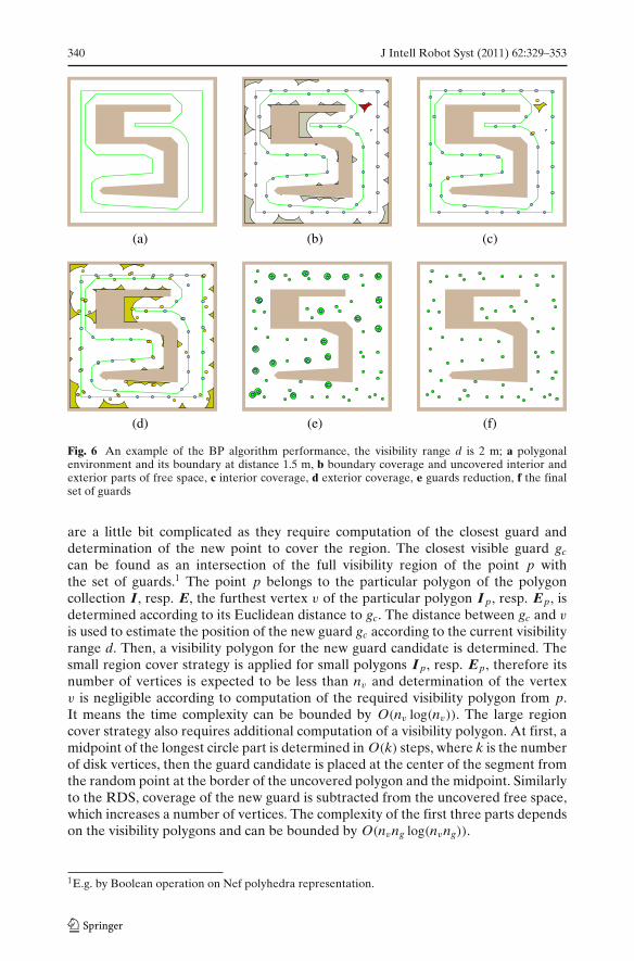
The performance of the BP algorithm mostly depends on the initial boundaryselection. The original idea of the BP algorithm expects the boundary at a distanceclose to the visibility range. If a boundary is created at a very small distance to thepolygon border the guards will be placed unnecessarily close to obstacles. On theother side, if a distance is relatively high, the boundary created from the shrunkfree space can be degenerated. In a degenerated case a large portion of the freespace is a part of the exterior and the heuristic approach is used. A boundary canbe determined as the border of the shrunk free space by a distance b . Duringexperimental verification of the proposed algorithm a set of b values have beenfound for each particular environment and visibility range, see Section 5. An exampleof the Boundary Placement algorithm performance is shown in Fig. 6.

Complexity of the algorithm is very similar to RDS. Assume that the number ofrandom samples in the first three parts is one and W is represented by nv vertices.The first part of the BP algorithm requires computation of a visibility polygon foreach new guard, which can be done in O(nv log nv). The second and third parts


(a) (b) (c)

(d) (e) (f)

Fig. 6 An example of the BP algorithm performance, the visibility range d is 2 m; a polygonalenvironment and its boundary at distance 1.5 m, b boundary coverage and uncovered interior andexterior parts of free space, c interior coverage, d exterior coverage, e guards reduction, f the finalset of guards

are a little bit complicated as they require computation of the closest guard anddetermination of the new point to cover the region. The closest visible guard gc

can be found as an intersection of the full visibility region of the point p withthe set of guards.1 The point p belongs to the particular polygon of the polygoncollection I, resp. E, the furthest vertex v of the particular polygon I p, resp. Ep, isdetermined according to its Euclidean distance to gc. The distance between gc and v

is used to estimate the position of the new guard gc according to the current visibilityrange d. Then, a visibility polygon for the new guard candidate is determined. Thesmall region cover strategy is applied for small polygons I p, resp. Ep, therefore itsnumber of vertices is expected to be less than nv and determination of the vertexv is negligible according to computation of the required visibility polygon from p.It means the time complexity can be bounded by O(nv log(nv)). The large regioncover strategy also requires additional computation of a visibility polygon. At first, amidpoint of the longest circle part is determined in O(k) steps, where k is the numberof disk vertices, then the guard candidate is placed at the center of the segment fromthe random point at the border of the uncovered polygon and the midpoint. Similarlyto the RDS, coverage of the new guard is subtracted from the uncovered free space,which increases a number of vertices. The complexity of the first three parts dependson the visibility polygons and can be bounded by O(nvng log(nvng)).

1E.g. by Boolean operation on Nef polyhedra representation.


Table 2 Basic properties ofused maps

Map Dimensions No. No. Reducedname (m × m) holes vertices no. vertices

jh 20.5 × 23.1 9 424 212ta 39.7 × 46.9 2 174 87pb 133.3 × 105.0 3 192 92

The last optimization procedure requires computation of mutually visible guards,which can be done in O((nv + ng)

2). All pairs can be sorted in O(n2g log(n2

g)), but onlyng/2 pairs can be selected at maximum and only ng/2 new guards can be determined,therefore complexity of the determination of visibility regions is not increased. Theoverall algorithm complexity can be bounded by O(nvng log(nvng) + n2

v + n2g log(n2

g)).The boundary, used in the first part of the algorithm, can be obtained as a border

of the shrunk free space. The shrunk free space can be found by the Minkowski sumof the free space polygon and a convex disk, therefore the boundary determinationcan be bounded by O((nvk)2), where nv is the number of polygon vertices and k isthe number of disk vertices.

5 Experiments

The performance of the three presented algorithms have been experimentally eval-uated within three maps of real environments.2 The assumed robot has differentialnonholonomic drive and free space has been shrunk by a radius of the circumscribedcircle around the robot polygonal shape, therefore a robot is modeled as a pointrobot. All maps3 have been filtered by the polygon filter technique presented inSection 4.1.1 for the relevance value r = 5 cm. Changes of the free space area is lessthan one percent after filtering. The environment properties are presented in Table 2and they are visualized in Fig. 7.

The performance of algorithms is evaluated for the set of visibility ranges {inf,10.0, 5.0, 4.0, 3.0, 2.0, 1.5, 1.0} meters, where inf denotes the unrestricted visibilityrange. The restricted visibility is modeled by a disk with 24 vertices.

Two qualities of the sensor placement solutions are examined, a number of foundguards and a length of the inspection path. The path is found as a solution of therelated TSP. The TSP is solved exactly by the Concorde solver [26] for all problems,except solutions for the map pb and visibility ranges d ∈ {1.0, 1.5} (all algorithms)and the map ta, d = 1.0 only in the case of the CPP algorithm. In these particularcases a number of guards is too high and the exact solution is too computationallydemanding. That is why these problems are solved by the Chained Lin-Kernighanheuristic [27].

The BP and RDS algorithms are randomized, therefore 20 solutions are foundby each algorithm for each particular configuration (map and visibility range) andaverage values are determined. To compute overall algorithm performance ratios of

2These environments were used as testing environments for real experiments in the search and rescuemissions during solution of the IST-2001-FET project number 38873—PeLoTe Building Presencethrough Localization for Hybrid Telematic Systems.3The maps are available at http://purl.org/faigl/planning.

http://purl.org/faigl/planning


(a) map jh (b) map ta (c) map pb

Fig. 7 Testing environments jh, ta and pb

the number of guards and the length of the path are used. Before the algorithmscomparison the most suitable settings for each algorithm have been found.

The CPP algorithm does not have any special parameters. The polygon filteringtechnique is useful, because the reduction of vertices leads to less number of guards.A number of vertices after the polygon filtering is shown in the last column ofTable 2.

The RDS algorithm depends on the number of random samples m. An overallresults according to reference for m = 1 are presented in Table 3. The m = 25provides the best performance while it is less computation intensive than highervalues of m.

The BP depends mainly on the boundary distance. For each map and visibilityrange the boundary distance b has been experimentally found, see Table 4. For smallvisibility ranges the boundary is in one meter from obstacles for all used maps, whilehigher visibility ranges require particular value of b for each map to get better results.Presented values do not provide the smallest number of found guards, but they havebeen selected to have small the total number of b values and the length of inspectionpaths. The number of random samples has been set to 1 and the heuristic parametersto μI = μE = 0.66.

A comparison of the algorithms is made according to reference solution found bythe CPP algorithm, it means that for each particular solution a number of guardsand a length of the tour are divided by appropriate values of the CPP solution. Theratios are denoted as GR for Guards Ratio and LR for Length Ratio. The relative

Table 3 RDS performanceaccording to the number ofrandom samples m

m Guards ratio Length ratio

1 1.00 1.005 0.88 0.9510 0.87 0.9425 0.87 0.9350 0.87 0.9375 0.88 0.93100 0.89 0.93


Table 4 Selected values of theboundary parameter b

Map Boundary distance b (m)

Visibility range d ≤ 2 m Visibility range d > 2 m

jh 1.0 1.5ta 1.0 3.0pb 1.0 2.0

values allow presentation of overall results as average values and sample standarddeviations σGR, σLR. The overall results of the RDS and BP algorithms are presentedin Table 5. In Fig. 8 the first two bars denote guards ratios and the next two barsdenote length ratios for the RDS and BP algorithms according to the referencesolution found by the CPP algorithm. Detail results are dedicated to Appendix A.

The RDS algorithm provides less number of guards than the CPP and also the pathis about 10% shorter. Similarly the BP outperforms the CPP. The ratios increase withdecreasing visibility range, but paths are more than about twenty percents shorter.For the unrestricted visibility range performances of the BP and RDS algorithms arepretty much similar, however for the visibility range 10 m the BP provides shortertour about more than 10%. For higher visibility ranges the difference in the numbersof guards is not so significant, but the BP still outperforms the RDS in the length ofthe inspection tour.

During the evaluation of the BP performance, it has been observed that theguards optimization procedure significantly reduces the number of required guards.The procedure can be used for any guard set, therefore solutions of the CPP andRDS have been optimized. The overall comparison as ratios according to the CPPalgorithm is presented in Table 6. The post-processed solutions are denoted as CPP-opt and RDS-opt and the BP algorithm without optimization as BP-notopt. Theoptimization procedure decreases numbers of guards for the CPP and RDS and tourlengths are also decreased. For the RDS the tour reduction is about three percents.An interesting observation provides results for the BP without optimization. How-ever the number of guards is reduced about 10% the length of the tour is shortenedonly about one percent after the optimization. This experimental results support themain idea of the BP algorithm to guide the sampling process and to place guards closeto each other to reduce the final length of the tour. The inspection path is still shorter

Table 5 Algorithmsperformance

d (m) RDS algorithm BP algorithm

GR LR σGR σLR GR LR σGR σLR

inf 0.38 0.76 0.05 0.05 0.38 0.77 0.05 0.0510.0 0.49 0.85 0.08 0.07 0.45 0.74 0.11 0.135.0 0.61 0.89 0.13 0.11 0.54 0.75 0.12 0.144.0 0.65 0.89 0.15 0.11 0.60 0.76 0.15 0.143.0 0.67 0.91 0.09 0.05 0.62 0.78 0.11 0.132.0 0.75 0.93 0.04 0.03 0.59 0.82 0.04 0.041.5 0.72 0.88 0.03 0.04 0.56 0.75 0.02 0.021.0 0.70 0.85 0.01 0.04 0.60 0.74 0.01 0.02


Fig. 8 The algorithmscomparison relatively to theCPP algorithm

10.0 5.0 3.0 2.0 1.0

Visibility range [m]

Rat

io0.

00.

20.

40.

60.

81.

0 Guards ratio: RDSBP

Length ratio: RDSBP

for solutions found by the BP-notopt, however the number of guards is higher thanfor the RDS-opt and CPP-opt in several cases.

To demonstrate capabilities of the presented algorithms several examples of foundsolutions for additional environments are presented in Appendix B.

5.1 Effect of Disturbances

A robot performing an inspection does not have precise localization nor sensors areperfect. The imperfect localization leads to miss the exact guards positions. Alsoparticular sensor coverage can be less than the expected one. These disturbancescan lead to imperfect coverage. It is clear that a solution with less number of sensinglocations for particular visibility range will be more sensitive to sensing locationsdisturbances or changes in the sensor visibility range. To examine the sensitivity ofsolutions found by the particular algorithm two experiments have been performed asfollows.

The effect of the localization error has been examined by a random perturbationof each sensing location of found solutions presented in the previous section. Theperturbation has been performed in two steps to reflect position estimation accuracyand repeatability. At first, the position of the guard has been modified according to

Table 6 Overall algorithmsperformance

Method GR LR σLR σGR

CPP 1.00 1.00 0.00 0.00RDS 0.62 0.87 0.08 0.15BP 0.54 0.76 0.10 0.12CPP-opt 0.74 0.91 0.04 0.03RDS-opt 0.53 0.84 0.08 0.12BP-notopt 0.64 0.77 0.11 0.18


(a) 98.9% coverage caused by localization imper-fections

(b) 87.8% coverage caused by 25% reduced visi-bility range

Fig. 9 Examples of disturbances to coverage, small disks represent guards, the guards beforedisturbances are in blue

two dimensional Gaussian distribution N (0, σ 2a ), where σa represents accuracy of the

localization. Such positions have been then modified according to N (0, σ 2r ), where

σr represents repeatability of the localization method. Computed coverage fromthese new positions has been expressed as the percentage of seen area of free space,denoted as %Coverage. An example of imperfect coverage is illustrated in Fig. 9a. Toget statistically meaningful results each found solution has been randomized 20 timesand average values of the coverage have been computed.4 Regarding to presentedresults of localization methods in [28], two sets of values of localization accuracyand repeatability have been considered for indoor environments. The methods arebased on visual landmarks and the accuracy is lower than for a method based on laserrange finder presented in [29], thus the selected values of coverage change representthe upper bounds. The total number of performed experiments for the positionperturbations is 39,360. The overall results are presented in Table 7. It is shown thatthe guard optimization procedure increases sensitivity of the solution to the positionperturbations. The coverage error is not significant for higher visibility ranges, evenfor the d = 1 m the error is less than 1.5% for more accurate localization method(σa = 14 cm). For σa = 30 cm the proposed BP algorithm without the optimizationprocedure provides competitive results to the RDS algorithm.

Sensitivity of the algorithm to disturbances of the visibility range d has beenexamined by a systematic decreasing of the sensor visibility range. A coverage ofa solution for the particular value of d has been computed for the decreased d andexpressed as the percentage of seen area similarly to the previous examination. An

4That means 480 sets of sensing localizations for the RDS, resp. BP, algorithm for each map andvisibility range.


Table 7 An effect of position disturbances

Method d = 1.0 m d = 5.0 m d = 10.0 m

%Coverage LR GR %Coverage LR GR %Coverage LR GR

Localization accuracy σa = 14 cm, localization repeatability σr = 8 cmCPP 99.95 0.97 1.00 100.00 1.00 1.00 100.00 1.00 1.00RDS 99.42 0.83 0.70 99.93 0.88 0.61 99.93 0.85 0.49BP 98.72 0.73 0.60 99.52 0.75 0.54 99.64 0.74 0.45CPP-opt 99.79 0.87 0.75 99.99 0.91 0.72 100.00 0.91 0.72RDS-opt 98.84 0.79 0.57 99.91 0.86 0.54 99.91 0.83 0.44BP-notopt 99.24 0.78 0.77 99.58 0.76 0.64 99.69 0.74 0.51

Localization accuracy σa = 30 cm, localization repeatability σr = 18 cmCPP 99.28 0.92 1.00 99.99 1.00 1.00 100.00 1.00 1.00RDS 97.05 0.81 0.70 99.50 0.88 0.61 99.46 0.84 0.49BP 95.45 0.73 0.60 98.56 0.75 0.54 98.78 0.74 0.45CPP-opt 98.05 0.83 0.75 99.86 0.91 0.72 99.95 0.91 0.72RDS-opt 94.94 0.76 0.57 99.26 0.86 0.54 99.33 0.83 0.44BP-notopt 97.44 0.79 0.77 98.69 0.76 0.64 98.87 0.75 0.51

example of such decreased coverage is shown in Fig. 9b. Results for the selectedvisibility ranges and particular reductions are presented in Table 8. A shortenedvisibility range about 10 cm (or less), which is higher disturbance than an accuracy ofavailable laser range finders, does not really affect the quality of coverage. Moreover,the accuracy can be considered in the requested visibility range and a solution of thesensor placement problem can be found for such reduced visibility range.

The presented results confirm the expectation that a solution with smaller numberof guards is more sensitive to disturbances. However, the cost of the solution (thenumber of guards and the length of the inspection path) have to be taken intoaccount in selection of the most suitable algorithm for particular robot configuration.In addition, the imperfections can be considered in the visibility range, thus a solutioncan be found for particularly smaller d. Hence, the disturbances are not a real issueand overall comparison of the algorithms, presented in Table 6, provides an overviewof expected quality of a found solution by the particular algorithm.

5.2 Required Computational Time

Beside the quality of solutions the required computational time is important for thereal applicability of the algorithms in the mobile robotics. The theoretical boundsprovide estimation of the complexity, however the real computational requirements

Table 8 An effect of visibility range disturbances, values of %Coverage

Method d = 1.0 m d = 5.0 m d = 10.0 m

d95% d90% d75% d98% d90% d80% d99% d90% d80%

CPP 100.00 99.99 99.40 100.00 99.95 99.73 100.00 100.00 99.99RDS 99.90 99.16 89.81 100.00 99.62 97.48 100.00 99.60 98.19BP 99.15 97.37 85.92 99.97 99.19 96.51 99.99 99.29 97.48CPP-opt 99.94 99.78 96.90 100.00 99.82 99.19 100.00 99.98 99.74RDS-opt 99.40 97.84 85.17 99.98 99.36 96.50 100.00 99.47 97.70BP-notopt 99.58 98.40 89.39 99.99 99.38 97.15 100.00 99.42 97.85


mainly depend on used geometric models. To compare the real requirements allexperiments have been performed in the same computational environment with theAthlon X2@2 GHz CPU, 1 GB RAM running FreeBSD 7.1 with only one CPU corededicated to computations.

The CPP algorithm has been implemented in C++ and CGAL library version3.3.1 [30]. The used geometric kernel has been Exact_predicates_exact_-constructions_kernel_with_sqrt, which provides sufficient precision and good real-time performance. The program has been compiled by the G++ 4.2 with the−O2 optimization flag. The required computational time linearly increases with anumber of found guards, see Fig. 10a. For problems with less than 500 guards thecomputation takes hundreds of milliseconds. The largest solved problem with 1,852guards has been solved in 3.3 s.

The RDS algorithm has been implemented in Java with the geometric libraryJTS [31] and the diablo-jdk1.6.0 [32] java runtime machine. The real-time per-

++++++++

+++++++++

++

++++

++++

+

++

+ +++ +

++

+

+

++

++

+

+

+

+

+

+

+ +

+

100 200 300 400 500

020

040

060

080

0

Number of guards

CPU

tim

e [m

s]

(a) CPP

0−100 100−200 200−300 300−400 400−500

Number of guards

CPU

tim

e [s

]

0.1

0.5

1.0

5.0

10.0

50.0

m=1m=5m=25m=50

(b) RDS

0−100 100−200 200−300 300−400 400−500

Number of guards

CPU

tim

e [s

]

1020

5010

020

050

010

0020

00

(c) BP

Fig. 10 The algorithms required computational time of the examined problems


formance is presented in Fig. 10b as a histogram of required computational timeaccording to the number of found guards, average values are visualized. For 25random samples a solution is found in several seconds, while for m = 1 it is found inhundreds of milliseconds (solutions with less than 300 guards). The used geometricrepresentation is double precision floating point (IEEE 754), which provides onlylimited precision of geometric operations. During the experiments, the total numberof failures (mainly in the intersection operation) has been 3,867, which represents0.560% of the total number of found guards or 0.015% of the total number ofperformed guards selections. The most problematic map is jh with 2,120 failures.For the map ta 1,378 failures has been recorded. The advantage of the randomizedincremental algorithm is safe recovery from such fails. If an operation cannot beperformed, a new random point is generated and the algorithm can continue.

An implementation of the BP algorithm is based on the Planar Nef polyhedrarepresentation, from the CGAL library version 3.1, which does not support simpledouble precision, therefore the precise CGAL::Gmpz kernel has been used. Thisrepresentation allows Boolean operations on polygons, which can be partially closed,i.e. an edge of the polygon border can be opened while the next edge can be closed.However the theoretical bound for the first three parts of the algorithm is lessthan for the RDS (only one random sample is used), the real computational timeis heavily affected by the used geometric kernel. During subtraction of polygons a lotof Steiner points are created and due to the used arbitrary precision representationthe polygonal operations are incredibly slow and the largest problem with morethan one thousands guards has been solved in two hours. Small problems with lessthan hundred guards are solved in tens of seconds. Running times are shown inFig. 10c, solutions with 300–400 guards are mostly found for small visibility ranges,therefore more Steiner points are created. The post-processing optimization takesabout twenty percent of the total required computational time. It should be notedthat all visibility polygons of found guards are re-computed in the optimizationprocedure.

6 Conclusion

The new randomized sensor placement algorithm called the Boundary Placementhas been presented. The proposed randomized sampling procedure explicitly usesknowledge about the environment shape to guide the randomization process. Perfor-mance of the proposed algorithm has been experimentally compared with two state-of-the-art algorithms. The algorithms have been evaluated according to the numberof found guards and the length of the inspection path. The proposed BP algorithmoutperforms both algorithms and provides solution with less number of guards andabout 10% shorter path. The experimental results show that length of the path can bedecreased by more sophisticated sampling even in cases that the decoupled problemsare solved independently.

However only restricted visibility range has been considered in the experiments,the proposed BP algorithm can be easily extented to consider the incident constraintslike the RDS. Applications of the RDS algorithm in the related VPP have beenreported in the literature, hence the applicability of the BP algorithm to all relatedproblems is expected, as it provides better solutions than the RDS.


The randomized approach provides solution of the sensor placement problemin less than few seconds, therefore it is suitable for real applications. Even thoughthe real computational requirements of the proposed BP algorithm are higher thanthe RDS, due to used precise geometry representation, the complexity of the BPalgorithm is lower then the RDS, because only one random sample and one pointfrom the heuristic is used for each found guard. The post-processing optimizationincreases the complexity, but overall performance of the BP without optimizationis similar to the RDS regarding to the number of guards and it provides shorterinspection paths. Also the optimization procedure is useful for the RDS as well asfor the CPP algorithm.

In the majority of the examined problems, more than 80% guards are placedon the boundary in the initial (the boundary cover part), which is very efficient,just one random sample is used. The boundary is created from the shrunk freespace, and the performance of the algorithm can be probably increased by structureslike the Visibility-Voronoi diagram [33] or Saturated Generalized Voronoi Diagram(SGVD) [34].

Appendix A: Experimental Results

Particular results for each examined environment are presented in Tables 9, 10and 11.

Table 9 Algorithmsperformance for the map jh

d (m) No. guards Length (m)

CPP RDS BP CPP RDS BP

inf 94 33 31 208 154 14910.0 95 37 32 207 158 1185.0 101 44 37 216 160 1244.0 106 47 41 220 164 1253.0 115 63 53 226 190 1382.0 175 126 94 282 269 2171.5 282 200 160 350 321 2581.0 552 388 340 471 414 359

Table 10 Algorithmsperformance for the map ta



inf 34 14 13 204 167 16710.0 35 18 15 203 176 1595.0 58 41 34 254 239 1974.0 72 54 52 272 260 2243.0 118 83 83 315 292 2662.0 231 170 139 408 366 3301.5 405 280 231 522 436 3861.0 865 598 526 746 595 528


Table 11 Algorithmsperformance for the map pb



inf 45 16 20 533 389 40710.0 73 41 44 613 567 5335.0 131 90 84 683 667 6194.0 160 120 109 720 697 6503.0 235 178 160 775 741 6962.0 434 349 271 902 851 7871.5 821 616 439 1,116 1,001 8581.0 1,809 1,289 1,067 1,565 1,346 1,151

Appendix B: Example of Solutions

Solutions for environments denoted as dense, potholes, warehouse and h2 are pre-sented in following figures (Figs. 11, 12, 13 and 14). All maps are processed by thepolygon filter with the relevance value 5 cm and the RDS has been run with m = 25.

(a) CPP, 285 guards, length 270 m (b) RDS, 61 guards, length 181 m (c) BP, 53 guards, length 180 m

Fig. 11 Example of solution for the map dense, 21 × 21 m, visibility range 4 m and boundary atdistance 0.5 m

(a) CPP, 306 guards, length 234 m (b) RDS, 81guards, length 159 m (c) BP, 68 guards, length 155 m

Fig. 12 Example of solution for the map potholes, 20 × 21 m, visibility range 2 m and boundary atdistance 1 m


(a) CPP, 361 guards, length 496 m (b) RDS, 99 guards, length 383 m (c) BP, 78 guards, length 363 m

Fig. 13 Example of solution for the map warehouse, 40 × 40 m, visibility range 4 m and boundary atdistance 1.2 m

(a) CPP, 361 guards, length 1353 m (b) RDS, 99 guards, length 1132 m

(c) BP, 78 guards, length 887 m

Fig. 14 Example of solution for the map h2 representing real building with dimensions approxi-mately 70 × 40 m, visibility range 5 m and boundary at distance 1.5 m

References

1. Chin, W.-P., Ntafos, S.: Optimum watchman routes. In: SCG ’86: Proceedings of the SecondAnnual Symposium on Computational Geometry, pp. 24–33, Yorktown Heights, New York.ACM (1986)

2. Packer, E.: Robust geometric computing and optimal visibility coverage. PhD thesis, StonyBrook University, New York (2008)


3. Danner, T., Kavraki, L.E.: Randomized planning for short inspection paths. In: Proceedings ofThe IEEE International Conference on Robotics and Automation (ICRA), pp. 971–976, SanFrancisco, CA. IEEE (2000)

4. Culberson, J.C., Reckhow, R.A.: Covering polygons is hard. J. Algorithms 17(1), 2–44 (1994)5. Tan, X., Hirata, T.: Finding shortest safari routes in simple polygons. Inf. Process. Lett. 87(4),

179–186 (2003)6. Ntafos, S.C.: Watchman routes under limited visibility. Comput. Geom. 1, 149–170 (1992)7. Li, F., Klette, R.: An approximate algorithm for solving the watchman route problem. In: RobVis,

pp. 189–206 (2008)8. Goodman, J.E., O’Rourke, J. (eds.): Handbook of Discrete and Computational Geometry. CRC

Press, Boca Raton (2004)9. González-Baños, H.H., Hsu, D., Latombe, J.-C.: Motion planning: recent developments. In: Ge,

S.S., Lewis, F.L. (eds.) Autonomous Mobile Robots: Sensing, Control, Decision-Making andApplications, Chapter 10. CRC (2006)

10. Wang, P.: View planning with combined view and travel cost. PhD thesis, Simon Fraser Univer-sity (2007)

11. González-Baños, H.H., Latombe, J.-C.: Planning robot motions for range-image acquisition andautomatic 3d model construction. In: AAAI Fall Symposium (1998)

12. Hörster, E., Lienhart, R.: On the optimal placement of multiple visual sensors. In: VSSN ’06: Pro-ceedings of the 4th ACM International Workshop on Video Surveillance and Sensor Networks,pp. 111–120, New York, NY. ACM (2006)

13. Erdem, U.M., Sclaroff, S.: Automated camera layout to satisfy task-specific and floor plan-specific coverage requirements. Comput. Vis. Image Underst. 103(3), 156–169 (2006)

14. Osais, Y.E., St-Hilaire, M., Yu, F.R.: Directional sensor placement with optimal sensing range,field of view and orientation. Mob. Netw. Appl. 15(2), 216–225 (2008)

15. Kazazakis, G.D., Argyros, A.A.: Fast positioning of limited visibility guards for the inspectionof 2d workspaces. In: Proceedings of the IEEE/RSJ Int. Conference on Intelligent Robots andSystems (IROS 2002), Lausanne (2002)

16. Scott, W.R., Roth, G., Rivest, J.-F.: View planning for automated three-dimensional objectreconstruction and inspection. ACM Comput. Surv. 35(1), 64–96 (2003)

17. Blaer, P.S., Allen, P.K.: Data acquisition and view planning for 3-d modeling tasks. In: IEEE/RSJInternational Conference on Intelligent Robots and Systems (IROS 2007), pp. 417–422, 29October–2 November 2007

18. Nüchter, A., Surmann, H., Hertzberg, J.: Planning robot motion for 3d digitalization of indoorenvironments. In: Proceedings of the 11th International Conference on Advanced Robotics(ICAR), pp. 222–227 (2003)

19. González-Baños, H.H., Latombe, J.-C.: Navigation strategies for exploring indoor environments.Int. J. Rob. Res. 21(10–11), 829–848 (2002)

20. González-Banos, H.H.: A randomized art-gallery algorithm for sensor placement. In: SCG ’01:Proceedings of the Seventeenth Annual Symposium on Computational Geometry, pp. 232–240.ACM, New York (2001)

21. Lavalle, S.M.: Planning Algorithms. Cambridge University Press (2006)22. Overmars, M.H., Welzl, E.: New methods for computing visibility graphs. In: SCG ’88: Proceed-

ings of the Fourth Annual Symposium on Computational Geometry, pp. 164–171. ACM, NewYork (1988)

23. Seidel, R.: A simple and fast incremental randomized algorithm for computing trapezoidaldecompositions and for triangulating polygons. Comput. Geom. Theory Appl. 1(1), 51–64 (1991)

24. Latecki, L.J., Lakämper, R.: Convexity rule for shape decomposition based on discrete contourevolution. Comput. Vis. Image Underst. 73(3), 441–454 (1999)

25. Wolter, D., Richter, K.-F.: Schematized aspect maps for robot guidance. In: Proceedings of theECAI Workshop Cognitive Robotics (CogRob) (2004)

26. Applegate, D., Bixby, R., Chvátal, V., Cook, W.: CONCORDE TSP Solver. http://www.tsp.gatech.edu/concorde.html (2003). Accessed 23 July 2010

27. Applegate, D., Cook, W., Rohe, A.: Chained lin-kernighan for large traveling salesman prob-lems. INFORMS J. Comput. 15(1), 82–92 (2003)

28. Chen, Z., Birchfield, S.T.: Qualitative vision-based path following. IEEE Transactions onRobotics 25(3), 749–754 (2009)

29. Sohn, H.J., Kim, B.K.: Vecslam: an efficient vector-based slam algorithm for indoor environ-ments. J. Intell. Robot. Syst. 56(3), 301–318 (2009)

http://www.tsp.gatech.edu/concorde.html

http://www.tsp.gatech.edu/concorde.html


30. CGAL—Computational Geometry Algorithms Library. http://www.cgal.org (2004). Accessed 23July 2010

31. JTS Topology Suite. http://www.vividsolutions.com/jts/jtshome.htm. Version 1.5 (2004). Ac-cessed 23 July 2010

32. Diablo Caffe JDK 1.6.0-7. http://www.freebsdfoundation.org/downloads/java.shtml (2009). Ac-cessed 23 July 2010

33. Wein, R., van den Berg, J.P., Halperin, D.: The visibility–voronoi complex and its applications.In: SCG ’05: Proceedings of the Twenty-First Annual Symposium on Computational Geometry,pp. 63–72. ACM, New York (2005)

34. Huang, W.H., Beevers, K.R.: Complete Topological Mapping with Sparse Sensing. TechnicalReport 6, Rensselaer Polytechnic Institute Department of Computer Science (2005)

http://www.cgal.org

http://www.vividsolutions.com/jts/jtshome.htm

http://www.freebsdfoundation.org/downloads/java.shtml

a sensor placement algorithm for a mobile robot...

Documents