A Shape-Independent-Method for PedestrianDetection with Far-Infrared-Images

Yajun Fang+, Keiichi Yamada+∗, Yoshiki Ninomiya*, Berthold Horn+, Ichiro Masaki++Intelligent Transportation Research Center, Microsystems Technology Labs

Massachusetts Institute of Technology, Cambridge, MA 02139, USA∗Toyota Central R &D Labs, Inc. Japan

yjfang@mit.edu, yamakei@mit.edu, nino@milab.tytlabs.co.jp, bkph@ai.mit.edu, masaki@mit.edu

Abstract

Night-time driving is more dangerous than day-time driving — particularly for older drivers. Three to four times as manydeaths occur at night than in the day time [1]. To improve safety of night driving, automatic pedestrian detection based on infraredimages has drawn increasing attention because pedestrians tend to stand out more against the background in infrared imagesthan they do in visible light images. Nevertheless, pedestrian detection is by no means trivial in infrared images — many of theknown difficulties carry over from visible light images, such as image variability occasioned by pedestrians being in different poses.Typically, several different pedestrian templates have to be used in order to deal with a range of poses. Furthermore, pedestriandetection is difficult because of poor infrared image quality (low resolution, low contrast, few distinguishable feature points, littletexture information, etc.) and misleading signals To address these problems, this paper introduces a shape-independent pedes-trian detection method. Our segmentation algorithm first estimates pedestrians’ horizontal locations through “Projection-based”horizontal segmentation, and then determines pedestrians’ vertical locations through “Brightness/Bodyline-based” vertical seg-mentation. Our classification method defines multi-dimensional histogram-, inertial-, and contrast-based classification features,which are shape-independent, complementary to one another, and capture the statistical similarities of image patches containingpedestrians with different poses. Thus, our pedestrian detection system needs only one pedestrian template — correspondingto a generic walking pose — and avoids brute-force search for pedestrians throughout whole images, which typically involvesbrightness-similarity-comparisons between candidate image patches and a multiplicity of pedestrian templates. Our pedestriandetection system is not based on tracking, nor does it depend on camera calibration to determine the relationship between anobject’s height and its vertical image locations. Thus, it is less restricted in applicability. Even if much work is still needed tobridge the gap between present pedestrian detection performance and the high reliability required for real-world applications, ourpedestrian detection system is straightforward and provides encouraging results in improving speed, reliability, and simplicity.

I. Introduction

Automatic detection of pedestrians at night has attracted more and more attention. Eighty percent of police reports [8]cited driver errors as the primary cause of vehicle crashes. Because depth perception, color recognition, and peripheralvision are all impaired after sundown, 3–4 times as many deaths occur during night-time driving than day-time driving.Also, people’s visual capabilities deteriorate substantially as they age, as is shown in figure 1, which compares the visualability of a driver of age 60 with those of a driver of age 20. A 50-year-old driver needs twice as much light to see asdoes a 30-year-old [1].

Fig. 1. Vision Degradation for Senior People. (Image Source: MIT Age Lab.)

To enhance safety, current night vision systems use infrared-cameras to provide visual aids projected on a heads-updisplay. In the long run, however, automatic pedestrian detection and warning is envisioned so that drivers can respondpromptly without being distracted by added gadgetry. Compared to the vast research on pedestrian detection basedon visible light images [2][3][5][14][16][19] as summarized in [11][12][18], work on infrared-based pedestrian detectionresearch [11][12][18] has just started. In an earlier paper [6], we systematically compared different properties of visibleand infrared images and noted several unique features of infrared-based pedestrian detection. In this paper, we furtherinvestigate the statistical properties of these features and introduce a novel “shape-independent” pedestrian detectionscheme including automatic pedestrian image size estimation and multi-dimensional shape-independent classification. In

this section, we first discuss how we evaluate detection performance, then review previous work and analyze challengesassociated with automatic pedestrian detection using infrared images. Finally we will discuss the advantages of ourdesign as well as differences from conventional methods.

A. Performance Index

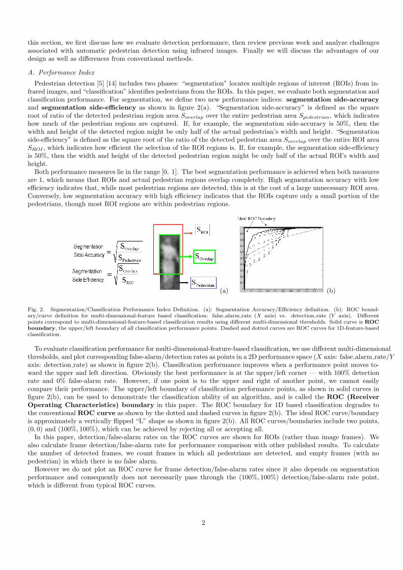
Pedestrian detection [5] [14] includes two phases: “segmentation” locates multiple regions of interest (ROIs) from in-frared images, and “classification” identifies pedestrians from the ROIs. In this paper, we evaluate both segmentation andclassification performance. For segmentation, we define two new performance indices: segmentation side-accuracyand segmentation side-efficiency as shown in figure 2(a). “Segmentation side-accuracy” is defined as the squareroot of ratio of the detected pedestrian region area Soverlap over the entire pedestrian area Spedestrian, which indicateshow much of the pedestrian regions are captured. If, for example, the segmentation side-accuracy is 50%, then thewidth and height of the detected region might be only half of the actual pedestrian’s width and height. “Segmentationside-efficiency” is defined as the square root of the ratio of the detected pedestrian area Soverlap over the entire ROI areaSROI , which indicates how efficient the selection of the ROI regions is. If, for example, the segmentation side-efficiencyis 50%, then the width and height of the detected pedestrian region might be only half of the actual ROI’s width andheight.

Both performance measures lie in the range [0, 1]. The best segmentation performance is achieved when both measuresare 1, which means that ROIs and actual pedestrian regions overlap completely. High segmentation accuracy with lowefficiency indicates that, while most pedestrian regions are detected, this is at the cost of a large unnecessary ROI area.Conversely, low segmentation accuracy with high efficiency indicates that the ROIs capture only a small portion of thepedestrians, though most ROI regions are within pedestrian regions.

(a) (b)

Fig. 2. Segmentation/Classification Performance Index Definition. (a): Segmentation Accuracy/Efficiency definition. (b): ROC bound-ary/curve definition for multi-dimensional-feature based classification: false alarm rate (X axis) vs. detection rate (Y axis). Differentpoints correspond to multi-dimensional-feature-based classification results using different multi-dimensional thresholds. Solid curve is ROCboundary, the upper/left boundary of all classification performance points. Dashed and dotted curves are ROC curves for 1D-feature-basedclassification.

To evaluate classification performance for multi-dimensional-feature-based classification, we use different multi-dimensionalthresholds, and plot corresponding false-alarm/detection rates as points in a 2D performance space (X axis: false alarm rate/Yaxis: detection rate) as shown in figure 2(b). Classification performance improves when a performance point moves to-ward the upper and left direction. Obviously the best performance is at the upper/left corner — with 100% detectionrate and 0% false-alarm rate. However, if one point is to the upper and right of another point, we cannot easilycompare their performance. The upper/left boundary of classification performance points, as shown in solid curves infigure 2(b), can be used to demonstrate the classification ability of an algorithm, and is called the ROC (ReceiverOperating Characteristics) boundary in this paper. The ROC boundary for 1D based classification degrades tothe conventional ROC curve as shown by the dotted and dashed curves in figure 2(b). The ideal ROC curve/boundaryis approximately a vertically flipped “L” shape as shown in figure 2(b). All ROC curves/boundaries include two points,(0, 0) and (100%, 100%), which can be achieved by rejecting all or accepting all.

In this paper, detection/false-alarm rates on the ROC curves are shown for ROIs (rather than image frames). Wealso calculate frame detection/false-alarm rate for performance comparison with other published results. To calculatethe number of detected frames, we count frames in which all pedestrians are detected, and empty frames (with nopedestrian) in which there is no false alarm.

However we do not plot an ROC curve for frame detection/false-alarm rates since it also depends on segmentationperformance and consequently does not necessarily pass through the (100%, 100%) detection/false-alarm rate point,which is different from typical ROC curves.

2

B. Challenges and Reviews for Pedestrian Detection with Infrared Images

Pedestrian detection using infrared images has its own advantages as well as disadvantages [6][11][12][18] when com-pared with detection using visible light images. In general, pedestrians emit more heat than static background objects,such as trees, roads, etc. In far-infrared images, pedestrian brightness tends to be less impacted by lighting, color,texture, and shadow information than it is in visible light imagery, and is generally also somewhat brighter than thebackground. However, infrared image intensities depend not only on object temperature but also on object surfaceproperties (emissivity, reflectivity, and transmissivity), surface orientation, wavelength, etc. Infrared images have theirown characteristics that lead to detection difficulties. First, non-pedestrian objects, such as, animals, vehicles, trans-formers, electric boxes, roads, construction areas, light poles, etc., produce additional “bright areas” in infrared images,especially in summer. These additional sources of image clutter make it impossible to reliably detect pedestrians basedonly on their brightness. Secondly, the image intensities of the same objects are not uniform. Pedestrian orientation,clothes, accessories (such as backpacks), etc., all have an impact on observed image intensity patterns. Body-trunk areasare generally darker than head and hand areas, especially when pedestrians wear heavy coats or carry backpacks. Theupper parts of light poles appear brighter than the lower parts because of contrast phenomena in typical far-infraredcameras. Non-homogeneous optical properties add to detection difficulties. Thirdly, most infrared image intensities havea smaller intensity range than do comparable visible images. This leads to low image quality: blur, poor resolutionand clarity, low foreground/background contrast, fewer feature points and less texture information, etc.

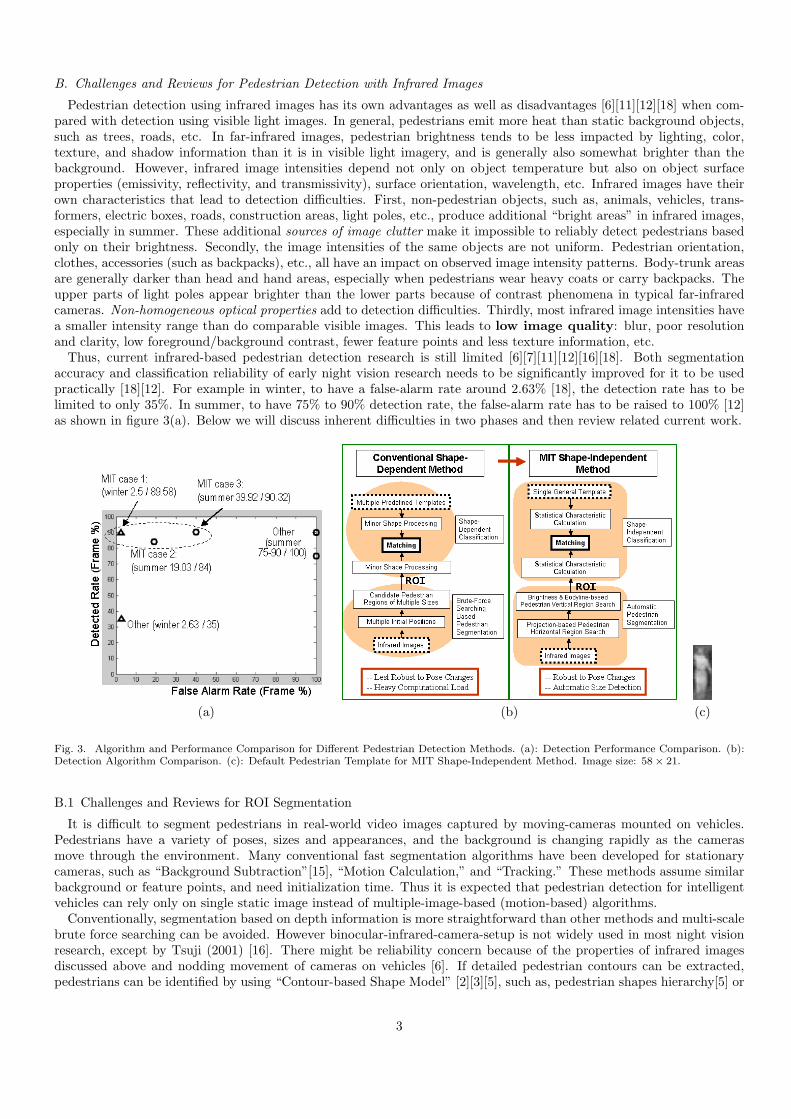
Thus, current infrared-based pedestrian detection research is still limited [6][7][11][12][16][18]. Both segmentationaccuracy and classification reliability of early night vision research needs to be significantly improved for it to be usedpractically [18][12]. For example in winter, to have a false-alarm rate around 2.63% [18], the detection rate has to belimited to only 35%. In summer, to have 75% to 90% detection rate, the false-alarm rate has to be raised to 100% [12]as shown in figure 3(a). Below we will discuss inherent difficulties in two phases and then review related current work.

(a) (b) (c)

Fig. 3. Algorithm and Performance Comparison for Different Pedestrian Detection Methods. (a): Detection Performance Comparison. (b):Detection Algorithm Comparison. (c): Default Pedestrian Template for MIT Shape-Independent Method. Image size: 58× 21.

B.1 Challenges and Reviews for ROI Segmentation

It is difficult to segment pedestrians in real-world video images captured by moving-cameras mounted on vehicles.Pedestrians have a variety of poses, sizes and appearances, and the background is changing rapidly as the camerasmove through the environment. Many conventional fast segmentation algorithms have been developed for stationarycameras, such as “Background Subtraction”[15], “Motion Calculation,” and “Tracking.” These methods assume similarbackground or feature points, and need initialization time. Thus it is expected that pedestrian detection for intelligentvehicles can rely only on single static image instead of multiple-image-based (motion-based) algorithms.

Conventionally, segmentation based on depth information is more straightforward than other methods and multi-scalebrute force searching can be avoided. However binocular-infrared-camera-setup is not widely used in most night visionresearch, except by Tsuji (2001) [16]. There might be reliability concern because of the properties of infrared imagesdiscussed above and nodding movement of cameras on vehicles [6]. If detailed pedestrian contours can be extracted,pedestrians can be identified by using “Contour-based Shape Model” [2][3][5], such as, pedestrian shapes hierarchy[5] or

3

human walking model[3]. Besides, “Human Component Features” [4][5][10][13][17], such as skin hue, eyes, faces, etc.,also help when segmenting pedestrians in visible images.

The above well known fast segmentation features are non-applicable to far-infrared images because of their uniqueproperties. It is also hard to segment pedestrians by grouping bright spots belonging to pedestrians based only ontheir pixel intensities. Using one fixed brightness threshold, for example, will lead to several separated bright spots atboth pedestrian regions and other noise resources, with results highly sensitive to the choice of brightness thresholds.If introducing “Template-Shape-based” multi-scale brute-force searching as some night vision algorithms do (as shownin Figure 3(b)), segmentation ROI outputs are all candidate pedestrian patches of different sizes and aspect ratios, atmultiple initial locations. The total number of ROIs for completely blind multi-scale brute force searching is as follows:

nROI =∑nscale

i=i nicenter−pos ∝ nrow ∗ ncolumn ∗ nscale (1)

where nscale is the number of scales in estimating pedestrian sizes, nicenter−pos is proportional to the image size (

nrow ∗ ncolumn ), which is the number of initial ROI center positions that must be tried when testing at different scales.The large search space for blind searching is a serious limitation in Different segmentation algorithms take advantage ofdifferent features to decrease nROI and to expedite the searching process. To decrease ncenter−pos, [18] searches brightand round regions as potential pedestrian heads in infrared images. [11] searches hot symmetrical ROIs with specificsize and aspect ratio based on the “Symmetry Property” of pedestrians and their brightness[9]. To decrease nscale,[18] and [11] assume flat roads so that pedestrians’ distance can be estimated based on pedestrians’ vertical positions inimages. [18] first detects road surface boundaries in order to estimate pedestrians’ sizes and height and remove impossiblepedestrian size/position combinations. [11] calibrates infrared cameras to build correspondences between image linesand distances in the 3D world for pedestrian size estimation. [12] does not make any assumptions and searches onlythree pedestrian sizes in a multi-scale brute force approach. The segmentation accuracy is limited compared with[11][18]. For real-world applications, segmentation algorithms need to further improve speed and accuracy and makefewer assumptions on the driving environment.

B.2 Challenges and Review for Classification

In far-infrared images, pedestrians yield widely varying image patterns because of the imaging complexity mentionedbefore and variations in pedestrian poses. When presented with multiple candidate image regions, differentiating pedes-trians from non-pedestrian regions is difficult. Typically the decision is made based on the similarity between ROI regionsand multiple pedestrian templates with various poses and appearances. Similarity can be computed either directly orindirectly. Typical direct methods compare image intensity pixel-by-pixel and compute the “Image-Intensity-Difference”between two patches, i.e., the Frobenius norm of image pixel intensity differences. The classification methods heavilydepend on shape matching and as a result are sensitive to segmentation errors and variations in pedestrian poses. [12]defines a template probabilistic model to encodes the shape information of pedestrians and the variations that the shapecan undergo by describing the possibility of foreground and background at each pixel based on training data. [11]identifies pedestrians through matching candidates with a simple model that encodes morphological characteristics ofa pedestrian. The shape-dependent filter removes candidates that do not present a human shape or are not as hot asexpected for a pedestrian. For indirect similarity-comparison, shape-dependent pedestrian-intensity-arrays are used totrain classifiers to capture the similarity between pedestrian training samples and ROIs, for example, support Vector Ma-chine [14] [18], Neural Network [13][19], Posteriori Detection (including Polynomial Classifiers, Multi-Layer Perceptrons,and Radial-basis Functions), etc., (as shown in figure 3(b)). [18] proposed SVM (support vector machine) classifiers forthree types of pedestrians for infrared images. These brightness-similarity-comparison based classification methods areshape-dependent, and might miss pedestrians with unusual poses even if multiple pedestrian-pose-templates or trainingsamples are used. Furthermore, complicated machine-learning methods require significant computational resources. Insummary, speed, reliability, and performance robustness to pose-changes and segmentation errors are serious concernsfor real-world night vision systems.

C. The Methodology and Principle for “Shape-Independent” Pedestrian Detection

Because of the above mentioned difficulties involved in shape dependent and/or brute-force searching based methods,the performance of present pedestrian detection systems is limited as shown in figure 3(a). In this paper, we introduce a“Shape-Independent” automatic pedestrian detection method with straightforward implementation. Figure 3(b) presentsthe major differences between our “shape-independent” methods and conventional “shape-dependent” methods. Thealgorithm can automatically estimate the horizontal location of candidate pedestrian regions to avoid brute-force multi-scale searching. Our novel classification feature vectors can characterize the statistical similarity of multiple pedestrianregions with different poses, and can also capture the statistical differences between pedestrian and non-pedestriansregions in infrared images. Thus, our multi-dimensional classification needs only one generic pedestrian template as

4

shown in figure 3(c) with size 58× 21 (details in section III). The method is based on the unique statistical propertiesof far-infrared images that we discovered through investigating the differences between visible and infrared images [6].

Our method has the following properties. First, it focuses on improving combined segmentation/classification systemsand balances the complexity and performance of two subsystems instead of maximizing one process while sacrificingthe other. This is because accurate segmentation can ease the classification task and robust classification can toleratesegmentation errors. Secondly, our segmentation procedure is robust to threshold choices. Finally, our algorithm doesnot make constraining assumptions for background, for example that flat roads; thus our results are very general. Theclassification performance comparison is shown in figure 3(a). For pedestrian detection in winter, we achieve a higherdetection rate when we set the false alarm rate to be similar to other available published results. For summer, we achievea lower false alarm rate when we set the detection rate to be similar to other available published results.

In the rest of the paper, we will introduce our “Automatic Pedestrian Segmentation,” and “Shape-IndependentMultiple Dimensional Classification” respectively in section II and III. Performance evaluation and future work will bediscussed in section IV and section V.

II. Automatic Pedestrian Segmentation

As mentioned in I-B.1, conventional “Template-Shape-based” segmentation involves searching with computationalload Ø(n2). We invented a new “horizontal-first, vertical-second” segmentation scheme involving only 1D searching invertical direction with computational load Ø(n). The method first automatically estimates the horizontal locations ofcandidate pedestrian regions, and then searches for pedestrians images vertically within the corresponding image stripes(from top to bottom in the images) at the estimated horizontal positions. Thus search space and computational loadare reduced significantly. In this section, we will respectively introduce our “horizontal segmentation” algorithm basedon “bright-pixel-vertical-projection curves,” and “vertical segmentation” based on “brightness/bodylines.”

A. Horizontal Segmentation

Here below we will first define the “bright-pixel-vertical-projection curve,” then explain how and why we can use thisconcept to estimate pedestrians’ horizontal locations.

A.1 Bright-pixel-vertical-projection Curves

For an infrared image, we define its bright-pixel-vertical-projection curves as the number of bright pixels inimage columns versus their corresponding horizontal positions. To count “Bright Pixels,” the intensity threshold isadaptively defined as follows:

Bright Pixel Threshold =max(Image Intensity) - Intensity Margin (2)

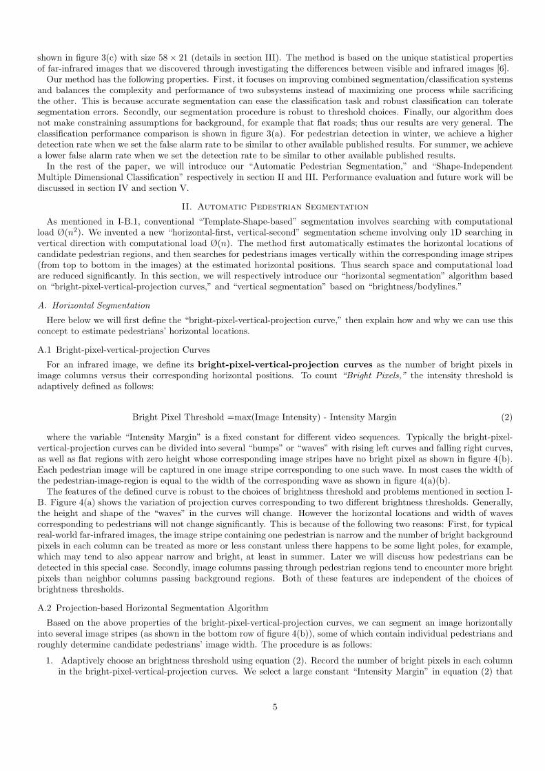
where the variable “Intensity Margin” is a fixed constant for different video sequences. Typically the bright-pixel-vertical-projection curves can be divided into several “bumps” or “waves” with rising left curves and falling right curves,as well as flat regions with zero height whose corresponding image stripes have no bright pixel as shown in figure 4(b).Each pedestrian image will be captured in one image stripe corresponding to one such wave. In most cases the width ofthe pedestrian-image-region is equal to the width of the corresponding wave as shown in figure 4(a)(b).

The features of the defined curve is robust to the choices of brightness threshold and problems mentioned in section I-B. Figure 4(a) shows the variation of projection curves corresponding to two different brightness thresholds. Generally,the height and shape of the “waves” in the curves will change. However the horizontal locations and width of wavescorresponding to pedestrians will not change significantly. This is because of the following two reasons: First, for typicalreal-world far-infrared images, the image stripe containing one pedestrian is narrow and the number of bright backgroundpixels in each column can be treated as more or less constant unless there happens to be some light poles, for example,which may tend to also appear narrow and bright, at least in summer. Later we will discuss how pedestrians can bedetected in this special case. Secondly, image columns passing through pedestrian regions tend to encounter more brightpixels than neighbor columns passing background regions. Both of these features are independent of the choices ofbrightness thresholds.

A.2 Projection-based Horizontal Segmentation Algorithm

Based on the above properties of the bright-pixel-vertical-projection curves, we can segment an image horizontallyinto several image stripes (as shown in the bottom row of figure 4(b)), some of which contain individual pedestrians androughly determine candidate pedestrians’ image width. The procedure is as follows:

1. Adaptively choose an brightness threshold using equation (2). Record the number of bright pixels in each columnin the bright-pixel-vertical-projection curves. We select a large constant “Intensity Margin” in equation (2) that

5

(a) (b)

(c) (d)

Fig. 4. The Feature of Bright-Pixel-Vertical-Projection Curves for Infrared Images and Brightness-based Vertical Segmentation Results.For (a)(c): Winter results. For (b)(d): Summer results. (a): Top row: original infrared image in winter. Center row and Bottom row:Bright-Pixel-Vertical-Projection curves when using two different thresholds. (b): Top row: original infrared image in summer. Center row:Bright-Pixel-Vertical-Projection Curve. Bottom row: Horizontally segmented image stripes based on projection curve. Note that Severalseparated stripes shown in the center row seem to be connected. For (c)(d): Brightness-based vertical segmentation results. For all projectioncurves: X axis: Image column position. Y axis: Number of bright pixels in each column.

makes the brightness threshold adaptively small to ensure that the image columns containing pedestrians will havenon-zero projection in the bright-pixel-vertical-projection curves.

2. Automatically search for the starting points of all rising curves (wave-start-points) and the ending points of allfalling curves (wave-end-points).

3. Separate the bright-pixel-vertical-projection curves into several waves by pairing wave-start-points and wave-end-points, and ignoring flat regions of zero height.

4. Record image stripes corresponding to these “waves.”

Because of background brightness “noises” in summer, projection curves for winter and summer images, as shownin figure 4(a)(b), have the following different properties. First, in winter, waves corresponding to pedestrians usuallyhave higher peaks than background waves, unlike summer where background “noises” may produce high wave peaks inprojection curves as shown in figure 4(b). Secondly, under complicated urban driving scenario in summer, as shown infigure 4(b), pedestrians and background brightness “noises” may be spatially proximate and their projection thus maymerge into one wave, which is the case for the second pedestrian from the left in figure 4(d). For winter images (example:sequence 1 shown in figure 17(a1)) and summer sequences in suburban area (example: sequence 2 in figure 17(b1)) withsparse foreground objects, pedestrian regions are less likely to be grouped with other “hot” foreground regions. In spiteof the differences that might make image stripes wider than the actual pedestrian image width in some cases, pedestrianswill be fully captured in individual horizontally separated stripes.

So far, we have presented a novel projection-based pedestrian pre-segmentation algorithm that horizontally separatesinfrared images into several image stripes that may contain pedestrians. In the next section, we will introduce how to

6

search pedestrians’ vertical location in segmented image stripes.

B. Vertical Segmentation within Horizontally Segmented Image Stripes

Here we will introduce two vertical segmentation algorithms. The first is a “Brightness-based” method (section II-B.1)that works best in winter and suburban situations where most segmented image stripes for pedestrians reflect the truewidth of pedestrian-image-regions. The second is a “Bodyline-based” method (section II-B.2) for more complicatedscenarios where the image stripes containing pedestrians might be wider than the pedestrian images true width. Thesetwo methods provide complementary results that work best in different scenarios, and the results from both methodsare sent to classification step to further improve reliability and accuracy.

B.1 Vertical Segmentation based on Brightness

After obtaining horizontally segmented image stripes from section II-A.2, the vertical positions of candidate pedestrianregions can be estimated by the highest and the lowest vertical locations of bright pixels within these stripes.

This method is applicable when the estimate of the pedestrian region width is reasonably accurate. In this case,most brightness-based vertical segmentation results for both winter and summer data turn out correctly as shown infigure 4(c)(d). Our classification algorithm has the ability to tolerate segmentation errors for pedestrian ROIs, such asthe inclusion of extra background regions or conversely missed portion, as shown in the first and the fourth pedestriansfrom the left in figure 4(c). Non-pedestrian ROIs have bright pixels at the boundaries, which facilitates the inertial-based classification algorithm to be described later in section III-B. When segmentation stripes are much wider thanthe actual pedestrian image size, ROIs may be much larger than the true width, as occurs for the third pedestrian fromthe right in figure 4(d). A “Bodyline-based” vertical segmentation algorithm (explained below) is proposed to improvesegmentation performance in such more difficult situations.

B.2 Vertical Segmentation based on Bodyline

In this method, we refine the pedestrian width estimation by detecting pedestrian regions’ left and right boundarypoints within segmented image stripes. Thus we can further search for pedestrians’ vertical positions based on a geometricpedestrian-size-model as described next.

For each row of image stripes, we define the portion of image rows within pedestrian regions as the pedestrian-bodyline, and define prominent feature points where image rows meet pedestrian boundaries as pedestrian-bodyline-terminals. Figure 5(a) presents one “bodyline” example in the waist area of a pedestrian image. Below we will describein detail how to detect bodyline, and how to vertically segment pedestrians within image stripes.

Step 1 Pedestrian Horizontal Bodyline Detection.

Because of infrared image features, in each row within segmented image stripes, the left pedestrian-bodyline-terminals are the points where image intensities change from darkness to brightness most rapidly. Similarly, at theright pedestrian-bodyline-terminals, image intensities change from brightness to darkness most rapidly. To obtainpedestrian-bodyline-terminals, we calculate intensity variation along the horizontal direction based on the modifiedSobel method as below:

∆I(x, y) = [I(x + 1, y + 1)− I(x− 1, y + 1) + 2I(x + 1, y)− 2I(x− 1, y) + I(x + 1, y − 1)− I(x− 1, y − 1)]/6 (3)

where (x, y) are pixel coordinates, I(x, y) is image intensity, and ∆I(x, y) is pixel-horizontal-spacing. We firstcalculate “pixel-horizontal-spacing” for all pixels in each row within horizontal segmentation stripes. Then wesearch in the left half portion of the row for a point with the largest “pixel-horizontal-spacing” as the candidate forthe left bodyline terminal points. We skip the row where “pixel-horizontal-spacing” for all pixels is smaller or equalto zero. Similarly, we determine the right bodyline terminal with the most negative “pixel-horizontal-spacing” inthe right half portion of the row. Thus we obtain two outmost boundaries and a bodyline for candidate pedestriansin each row within horizontal segmentation stripes. For segmented image stripes shown in figure 4(b), figure 5(b)preserves all pixels within detected candidate bodylines, in which pedestrians stand out and the background pixelssurrounding the pedestrian regions has been removed. It may happen that some boundary points belong to other“hot objects” next to the pedestrians, and we might not obtain a clear bodyline at every row of pedestrian regions.However, as long as we can obtain one bodyline, in the next step we can still estimate the candidate pedestrian’simage size based on the bodyline length.

Step 2 Pedestrian Location Estimation based on Pedestrian-Bodyline Matching

In figure 5(a), we propose a geometric pedestrian-size-model that defines one pedestrian’s size and location basedon the location and length of a waist-bodyline. The reason we use waist-bodylines is because the contrast between

7

human hip areas and their local background neighborhoods tend to be robust to the poses of walking pedestrians.Horizontal waist-bodylines are more likely to be detected and are not easily missed under a variety of conditions.Using the model, we can define multiple candidate pedestrian regions by assuming each detected bodyline to be thewaist-bodyline of an pedestrian. Figure 5(c) provides an example of bodyline-based pedestrian location estimation.A few estimated candidate pedestrian regions are marked.

Step 3 Histogram-based Bodyline/Pedestrian Searching

Among multiple candidate regions defined previously within a vertical image stripe, there is at most one actualpedestrian image region. Choosing one candidate pedestrian region is essentially a classification problem. We firstuse one histogram-based classification feature to search for the best candidate within each image stripe. Afterobtaining one candidate for each image stripe, we further determine whether it is a actual pedestrian image usingmulti-dimensional classification features explained in the next section. Details of the histogram-based feature andother classification features will be explained in section III. It is worth mentioning that we do not need to usea threshold in the searching process since we choose ROIs that are closest to our default pedestrian template(figure 3(c)) in histogram feature space.

(a) (b) (c) (d)

Fig. 5. Pedestrian segmentation based on two different methods. (a): Bodyline based geometric pedestrian-size-model. (b): Bodyline image.(c): Candidate pedestrian region estimation based on (a) and (b). (d): Bodyline-based segmentation result.

For initial horizontally segmented image stripes in the bottom row of figure 4(b), the bodyline-based vertical seg-mentation result is shown in figure 5(d), which provide more accurate segmentation results than the “brightness-basedsegmentation” results shown in figure 4(d) where background noise causes segmentation errors.

In sum, the flowchart of automatic pedestrian segmentation starts with “projection-based” horizontal segmentation asshown in figure 3(b). Within segmented image stripes, “brightness-based” vertical segmentation assumes that pedestrianpixels are brighter than the rest of background pixels in the image stripes. The “bodyline-based” method assumes thereexists clear brightness contrast between pedestrian image regions and their horizontal-neighbor-regions, and searchfor the left-positive/right-negative vertical-edge-pairs with high “pixel-horizontal-spacing” in order to detect potentialpedestrian bodylines and estimate candidate pedestrian positions. Both methods automatically estimate pedestrians’sizes and avoid multi-scale brute force searching. The first method is straightforward and works reliably in suburbansummer cases as well as winter cases. The second method works in complicated urban driving situations. Neithermethod needs to assume flat roads and both can work in a general driving situation. In real-world applications, bothsegmentation results will be fused in classification.

Conventional segmentation involves brute force searching within an entire image and produces multiple initial ROIsas in equation (1). Instead, “bodyline-based” segmentation involves only searching among multiple bodylines withinhorizontally segmented image stripes and the number of produced initial ROIs is as follows:

nbodyline ROI ≈ nimage stripe ∗ nbodyline (4)

where nimage stripe is the number of horizontally segmented image stripes and is usually less than 20 (even less thanthe number of image columns), and nbodyline is the largest number of bodylines in segmented image stripes and is muchless than the number of image rows. Thus nbodyline ROI is significantly less than in equation (1). The number of ROIs for“brightness-based” segmentation is equal to nimage stripe. In sum, our vertical segmentation produces fewer candidateROIs.

III. Classification

To recognize pedestrians, conventional classification is based on brightness-similarity-comparisons between ROIs andmultiple templates, which is shape-dependent and is subject to segmentation errors and pose-changes as mentioned in

8

section I-B.2. For robustness and reliability, we propose innovative classification that is based on comparing the similaritybetween multi-dimensional shape-independent feature vectors for ROIs and for one generic pedestrian template. Inthis section we first introduce histogram-, inertial-, and contrast-based classification features individually, then wewill propose our multi-dimensional classification methods and compare the classification ability of our defined shape-independent features with conventional shape-dependent features.

A. Histogram-based Classification

In this section we discuss the brightness histogram similarities among pedestrian regions with various poses, sizes andappearances, and introduce the histogram-feature’s ability to separate pedestrian/non-pedestrian ROIs based on onegeneric pedestrian template.

A.1 Statistical Similarity of Brightness Histograms for Pedestrian ROIs

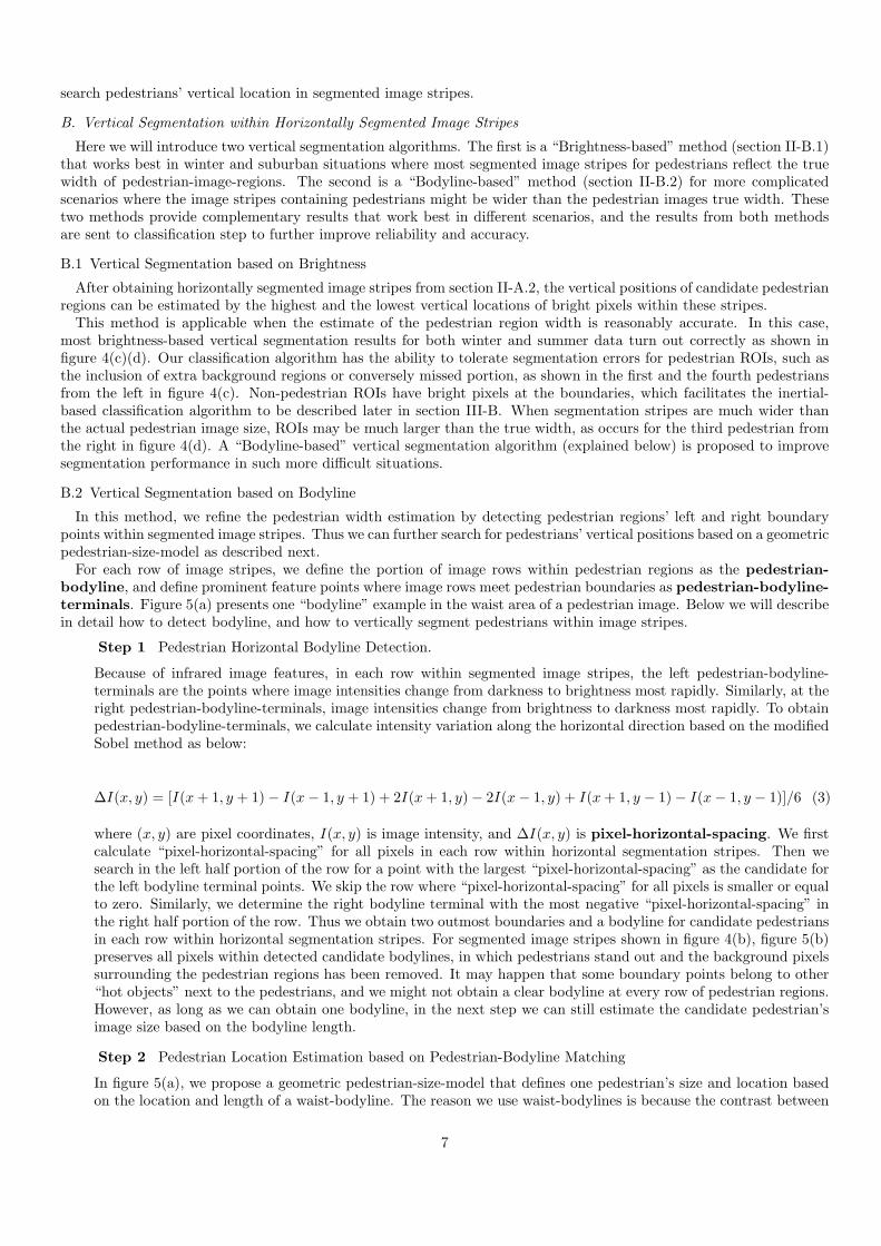
In section I-B, we have mentioned that pedestrian regions in infrared images are complex and not homogeneous.However, when pedestrians change poses, the intensity patterns should be consistent for similar body areas in differentinfrared images. Because of similar body temperatures and similar pedestrian surface properties, this observation appliesnot only for the same pedestrian of different poses, but also for different pedestrians with different gender, clothing,and in different seasons. Thus, there exists the similarity among image-brightness-histogram-curves for pedestrianpatches containing different people, with different poses, and in different seasons. This property is demonstrated inhistogram curve comparison in figure 6. Figure 6(a0) is our default pedestrian template cut from a summer sequence.Figure 6(a1) shows seven pedestrian ROIs from four winter images, in which pedestrians have different poses andare of different gender. Figure 6(b1) demonstrates the similarity among the brightness-histogram-curves for the sevenpedestrian regions. Figure 6(c1) compares the average brightness-histogram-curves of the above seven pedestrian regionsfrom winter images(solid line) with the histogram curve for the pedestrian template from summer images(dashed line)in figure 6(a0).

We further demonstrate statistical histogram similarity for pedestrian regions through the variation of brightness-histogram-curves from 911 rectangular pedestrian regions in seven different driving sequences. Figure 7(a) shows theexamples of pedestrian appearances and sizes in two sample sequences. We normalize all pedestrian patches to a standardsize [58× 21] (1218 pixels) before calculating their smoothed brightness-histogram-curves, i.e., histmROI(i), which is thenumber of pixels with brightness i. Figure 7(b) defines the “histogram variation curve,” i.e., the distribution of histogramvariation value hm(i)−hn(i) for all brightness i. In this way, the variation of all 911 histogram curves histmROI from theiraverage histogram histmean is presented as the collective “histogram variation curve” in figure 7(c), which resembles aGaussian shape (of zero mean) with certain skewness. We can see that most histogram shape variation is within [-10, 10]pixels, which is only 8.2% of the largest variation (1218 pixels). The fact provides us statistical evidence that histogramcurves for pedestrian regions are very similar.

A.2 The Classification Ability of Histogram Feature

Figure 6(b2) shows the comparison among all histogram curves for non-pedestrian ROIs in figure 6(a2), and figure 6(c2)shows the comparison between their average and the brightness histogram of a summer pedestrian template, as shown infigure 6(a0). The results are drawn with the same scale as figure 6(b1)(c1) with similar comparisons for pedestrian ROIs.The comparison between figure 6 (b) and (c) reveals that histogram features for pedestrian/non-pedestrian ROIs aredifferent in most cases. Because of the histogram similarity for pedestrian regions, as well as histogram differences be-tween pedestrian ROIs and non-pedestrian ROIs, pedestrians can be identified through histogram-similarity-comparisonbetween ROIs and one generic pedestrian template. Without losing generality, we choose figure 6(a0) as our genericpedestrian template. The Histogram Difference index is defined as the weighted summation for the square of bright-ness histogram difference at each brightness i as below:

Histogram Difference = α∑255

i=1 weight(i) ∗ [histROI(i)− histtemplate(i)]2 (5)

where histROI and histtemplate are histogram curves for ROIs and a template respectively, α is normalization coeffi-cient, weight(i) is weighting function that is fixed for all classification calculations. Typically segmentation errors mightintroduce extra dark background or bright regions, leading to higher histogram curve peaks at small/large brightnessvalue. Weight(i) is set to be small when brightness i is very dark or bright in order to reduce the impact of segmentationerrors. The expected value for pedestrian ROIs is 0. The larger the histogram difference for an ROI, the less likely isthe ROI to be a pedestrian.

B. Inertial-based Classification

Inertial-based classification feature is based on the inertial similarity among pedestrian regions, and is also shape-independent. We define inertial value for one image patch as in equation (6):

9

(a0) (a1) (a2)

50 100 150 200 2500

20

40

60

80

100

(b1) 50 100 150 200 2500

20

40

60

80

100

(b2)

50 100 150 200 2500

5

10

15

20

(c1) 50 100 150 200 2500

5

10

15

20

(c2)

Fig. 6. Properties of Brightness-histogram-curves for Pedestrian/non-Pedestrian ROIs. (a0): Pedestrian from summer data. Used as defaulttemplate in our algorithm. (a1): Pedestrian ROIs with different poses. (a2): Non-pedestrian ROIs. (a1)(a2) are segmentation results forwinter data. For (b1)(b2): Brightness histograms for (a1)(a2). (b1): demonstrates histogram similarity among winter pedestrian ROIs.(b2): demonstrates the histogram variation among winter non-pedestrian ROIs. For (c1)(c2): Solid lines: Average brightness histogram forwinter pedestrian ROIs (b1) and winter non-pedestrian ROIs (b2) respectively. Dashed lines: Histogram curve for summer pedestrian (a0).(c1): demonstrates the histogram similarity between winter pedestrians and summer pedestrian template. (c2): demonstrates the disparitybetween winter non-pedestrian ROIs and summer pedestrian template. For (b1)(b2)(c1)(c2): X axis: Image intensity range (0-255). Y axis:brightness histogram.

image inertial =

∑x,y I(x, y)d(x, y)2∑

x,y Itemplate(x, y)dtemplate(x, y)2(6)

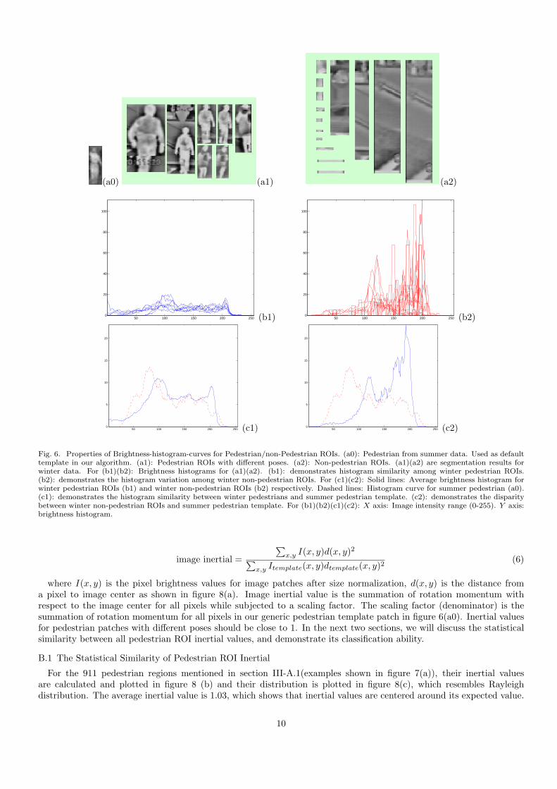
where I(x, y) is the pixel brightness values for image patches after size normalization, d(x, y) is the distance froma pixel to image center as shown in figure 8(a). Image inertial value is the summation of rotation momentum withrespect to the image center for all pixels while subjected to a scaling factor. The scaling factor (denominator) is thesummation of rotation momentum for all pixels in our generic pedestrian template patch in figure 6(a0). Inertial valuesfor pedestrian patches with different poses should be close to 1. In the next two sections, we will discuss the statisticalsimilarity between all pedestrian ROI inertial values, and demonstrate its classification ability.

B.1 The Statistical Similarity of Pedestrian ROI Inertial

For the 911 pedestrian regions mentioned in section III-A.1(examples shown in figure 7(a)), their inertial valuesare calculated and plotted in figure 8 (b) and their distribution is plotted in figure 8(c), which resembles Rayleighdistribution. The average inertial value is 1.03, which shows that inertial values are centered around its expected value.

10

(a1) (a2)

(b) (c)

Fig. 7. For (a1)(a2): Sample pedestrian regions from 2 sequences (every five frames) to show the variation of pedestrian poses and sizes,which correspond to the 2nd and 3rd pedestrian detection examples in section IV. (b): Left: two brightness-histogram-curves with brightnessi (X axis) vs. hn(i) and hm(i) (Y axis ) that are pixel numbers with brightness i from two image regions. Right: Definition for “histogramvariation curve” with all possible histogram variance value hn(i)−hm(i) (X axis) vs. variation frequency (Y axis). (c): Collective “histogramsvariation curve” for 911 pedestrian samples (in 7 sequences), with all possible histogram variation value (X axis) vs. the distribution ofhistogram variation value from all pedestrian histogram curves and their mean (Y axis).

Around 70% of pedestrian regions have inertial values within 0.8−1.2, around 94% of inertial values vary within 0.6−1.4.Figure 8(b) and (c) demonstrate inertial similarity for pedestrian regions in infrared images.

B.2 The Classification Ability of Inertial Feature

The inertial-based feature helps to remove classification ambiguity based on the histogram feature alone. Based on oursegmentation algorithm, when pedestrian/non-pedestrian ROIs have similar brightness histograms, ROIs have similarnumbers of bright pixels and some bright pixels must situate around image boundaries. For typical pedestrian ROIs,most bright pixels stay in the middle of image patches and only a few pixels at heads, hands, and feet areas touchhorizontal and vertical boundaries. For typical non-pedestrian ROIs, bright pixels are less centralized with more brightpixels near horizontal and vertical boundaries, leading to different inertial values. As shown in figure 8(a) the inertialvalue for the right non-pedestrian patch is larger than the left pedestrian patch despite their similar histogram feature.

C. Contrast-based Classification

In infrared images, there exists brightness contrast between pedestrian regions and their horizontal and verticalneighborhoods. The horizontal brightness contrast has been used in our segmentation algorithm to obtain pedestri-ans’ left/right boundaries. Because of the concern of robustness, the vertical contrast is not directly used to identifypedestrians in segmentation. Instead, it can be used to identify non-pedestrian as follows.

We evaluate the contrast between an ROI and its vertical neighborhoods by comparing the vertical edges within theseregions as shown in figure 9(a)(b). Vertical edges are defined as the image pixels with “pixel-horizontal-spacing”(defined in equation (3), section II-B.2) larger than a constant threshold. For a rectangular ROI, its upper/lowervertical neighborhood is a rectangular region that is right above/below the ROI with the same column width and

11

(a) hspace.2in (b) hspace.2in (c)

Fig. 8. (a): ROI inertial definition. (b): Collective inertial values for all 911 pedestrian samples. X axis: Pedestrian sample order. Y axis:Inertial feature value. (c): Distribution for inertial values in (b). X axis: Inertial value. Y axis: Distribution percentage.

half the ROI height. The Row-edge index for a rectangular region is defined as the average number of vertical edgepixels for each row of the region. Rich texture leads to a large row-edge index. The row-edge indices for an ROI andits upper and lower vertical neighborhoods are respectively called ROI row-edge index, upper row-edge index,and lower row-edge index. These three variables are defined as ROI contrast-feature vectors. For an ROI,the comparison between its ROI row-edge index and upper/lower row-edge index provides vertical texture contrastinformation between the ROI and its vertical neighborhoods.

For typical infrared images from real driving scenes, image stripes containing one pedestrian are narrow. Withoutlosing generality, we assume there is no pedestrian at the top of another pedestrian region within one segmented imagestripe. For pedestrian ROIs, the vertical neighborhoods are background whose vertical edges should be limited withinnarrow image stripes. Specifically, their lower vertical neighborhoods contain road areas, in which we cannot find twolong vertical lines or many vertical edge pixels beneath pedestrian ROIs. There is at most one vertical line produced bylane markers within narrow image stripes because of camera perspective, thus “Lower row-edge index” for pedestrianROIs should not be larger than 1. If this is not the case, non-pedestrian ROIs can be identified since pedestrian ROIspresent vertical contrast between ROIs and their lower neighborhoods.

Similarly, in most cases, the upper row-edge indices for pedestrian ROIs should be smaller than 2 since their “uppervertical neighborhoods” contain general sky, building, trees, etc., and none of them produces two (or more than two)adjacent vertical long edges within the narrow stripes of infrared-images. The exception is when pedestrians stand rightin front of “hot” light poles, which makes their upper row-edge indices be close to 2. In this case, we check their ROIrow-edge indices, which should be smaller than 2 for pedestrian ROIs, because some pedestrian image rows do nothave any vertical edge pixel and other rows contain at most two vertical edge pixels, i.e., pedestrian-bodyline-terminals.Thus, if both the upper row-edge indices and the ROI row-edge indices are large, there is no vertical contrast for ROIs,and non-pedestrian ROIs can be identified. The selected non-pedestrian ROIs are very likely to be in the middle oflight poles, which is the case for all selected non-pedestrian ROIs in figure 9(a) that correspond to poles in figure 5(d).The “ROI row-edge index” is used to remove the ambiguity between non-pedestrian ROIs containing light poles andpedestrian ROIs in front of poles.

In summary, pedestrian ROIs and their vertical neighborhoods should present vertical contrast and lead to small“upper/lower row-edge indices.” Though we cannot identify pedestrian ROIs simply based on vertical contrast, a fewnon-pedestrian ROIs can be identified and removed when vertical contrast does not exist based on one of the twofollowing conditions:

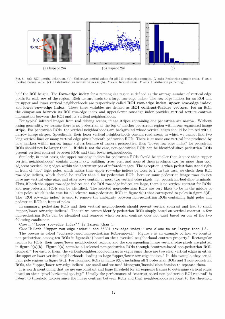
Case I: ‘‘Lower row-edge index’’ is larger than 1.Case II: Both ‘‘upper row-edge index’’ and ‘‘ROI row-edge index’’ are close to or larger than 1.5.The process is called “contrast-based non-pedestrian ROI-removal.” Figure 9 is an example of how we identify

non-pedestrians among ten ROIs in figure 5(d) based on their “vertical-neighborhood-contrast property.” Rectangularregions for ROIs, their upper/lower neighborhood regions, and the corresponding image vertical edge pixels are plottedin figure 9(a)(b). Figure 9(a) contains all selected non-pedestrian ROIs through “contrast-based non-pedestrian ROI-removal.” For each of them, the vertical-neighborhood-contrast is vague since there are two clear vertical edges in eitherthe upper or lower vertical neighborhoods, leading to large “upper/lower row-edge indices.” In this example, they are alllight pole regions in figure 5(d). For remained ROIs in figure 9(b), including all 3 pedestrian ROIs and 3 non-pedestrianROIs, the “upper/lower row-edge indices” are small and we need histogram/inertial classification to separate them.

It is worth mentioning that we use one constant and large threshold for all sequence frames to determine vertical edgesbased on their “pixel-horizontal-spacing.” Usually the performance of “contrast-based non-pedestrian ROI-removal” isrobust to threshold choices since the image contrast between ROIs and their neighborhoods is robust to the threshold

12

choices. In the worst case that a threshold is too large, both “ROI row-edge indices” and “upper/lower row-edge indices”for non-pedestrian ROIs are small and the non-pedestrian ROIs cannot be removed based on the two above conditions.It is acceptable since further histogram/inertial-based classification can identify them.

(a) (b) (c)

Fig. 9. “Contrast-based non-Pedestrian ROI Removal” for ROIs in Figure 5(d). For (a)(b): ROIs and their vertical neighborhood regionson edge map, i.e., vertical-neighborhood-contrast property. (a): For detected non-pedestrian ROIs. (b): For remained ROIs. (c): RemainedROIs on the original image.

C.1 Statistical Distributions of Contrast-based Classification Feature

(a) (b)

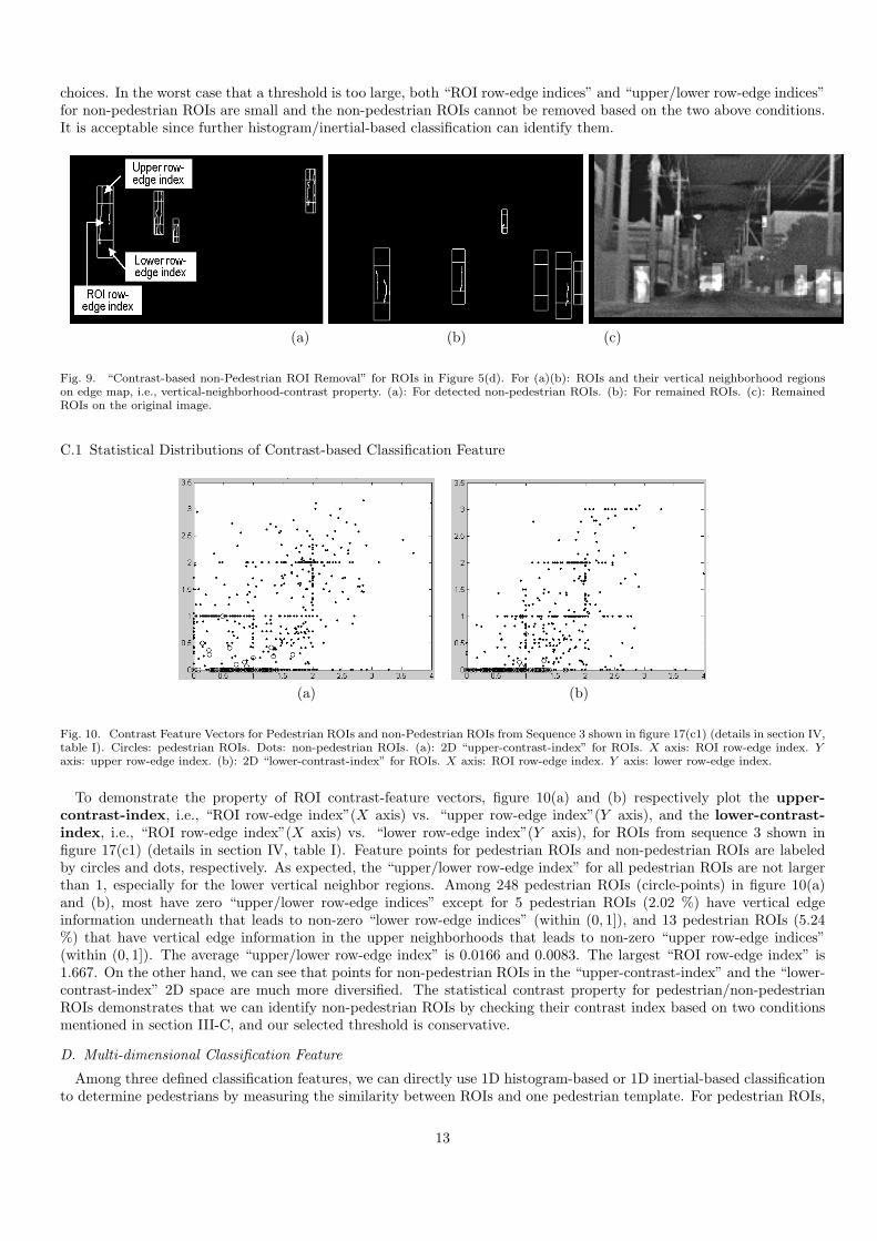
Fig. 10. Contrast Feature Vectors for Pedestrian ROIs and non-Pedestrian ROIs from Sequence 3 shown in figure 17(c1) (details in section IV,table I). Circles: pedestrian ROIs. Dots: non-pedestrian ROIs. (a): 2D “upper-contrast-index” for ROIs. X axis: ROI row-edge index. Yaxis: upper row-edge index. (b): 2D “lower-contrast-index” for ROIs. X axis: ROI row-edge index. Y axis: lower row-edge index.

To demonstrate the property of ROI contrast-feature vectors, figure 10(a) and (b) respectively plot the upper-contrast-index, i.e., “ROI row-edge index”(X axis) vs. “upper row-edge index”(Y axis), and the lower-contrast-index, i.e., “ROI row-edge index”(X axis) vs. “lower row-edge index”(Y axis), for ROIs from sequence 3 shown infigure 17(c1) (details in section IV, table I). Feature points for pedestrian ROIs and non-pedestrian ROIs are labeledby circles and dots, respectively. As expected, the “upper/lower row-edge index” for all pedestrian ROIs are not largerthan 1, especially for the lower vertical neighbor regions. Among 248 pedestrian ROIs (circle-points) in figure 10(a)and (b), most have zero “upper/lower row-edge indices” except for 5 pedestrian ROIs (2.02 %) have vertical edgeinformation underneath that leads to non-zero “lower row-edge indices” (within (0, 1]), and 13 pedestrian ROIs (5.24%) that have vertical edge information in the upper neighborhoods that leads to non-zero “upper row-edge indices”(within (0, 1]). The average “upper/lower row-edge index” is 0.0166 and 0.0083. The largest “ROI row-edge index” is1.667. On the other hand, we can see that points for non-pedestrian ROIs in the “upper-contrast-index” and the “lower-contrast-index” 2D space are much more diversified. The statistical contrast property for pedestrian/non-pedestrianROIs demonstrates that we can identify non-pedestrian ROIs by checking their contrast index based on two conditionsmentioned in section III-C, and our selected threshold is conservative.

D. Multi-dimensional Classification Feature

Among three defined classification features, we can directly use 1D histogram-based or 1D inertial-based classificationto determine pedestrians by measuring the similarity between ROIs and one pedestrian template. For pedestrian ROIs,

13

the expected histogram feature index should be close to 0, and the inertial feature index should be close to 1. Thefarther the histogram or inertial feature of an ROI deviates from its expected value, the less likely is the ROI to be apedestrian. Because “contrast-based non-pedestrian ROI-removal” is best at distinguishing non-pedestrian ROIs lackingin vertical contrast, the contrast-based feature has to be combined with other classification features.

Classification results based on 1D histogram feature alone can be very close to the ideal ROC boundary for wintersequences as shown in figure16(a)(details in section IV). To improve classification performance in complicated scenarios,we propose multi-dimensional classification methods. We first introduce 2D histogram/inertial-based classification insection III-D.1 in which the inertial feature helps to remove ambiguity introduced in 1D histogram-based classifica-tion as mentioned in section III-B.2.In section III-D.2, we introduce 3D histogram/inertial/contrast-based classificationthat involves “contrast-based non-pedestrian ROI-removal” to further decrease the ambiguity associated with 2D his-togram/inertial classification.

D.1 2D Histogram/Inertial-based Classification

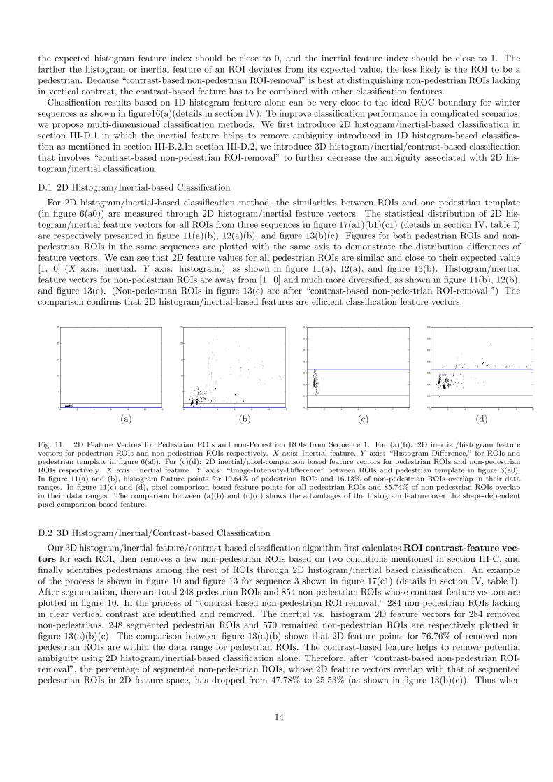
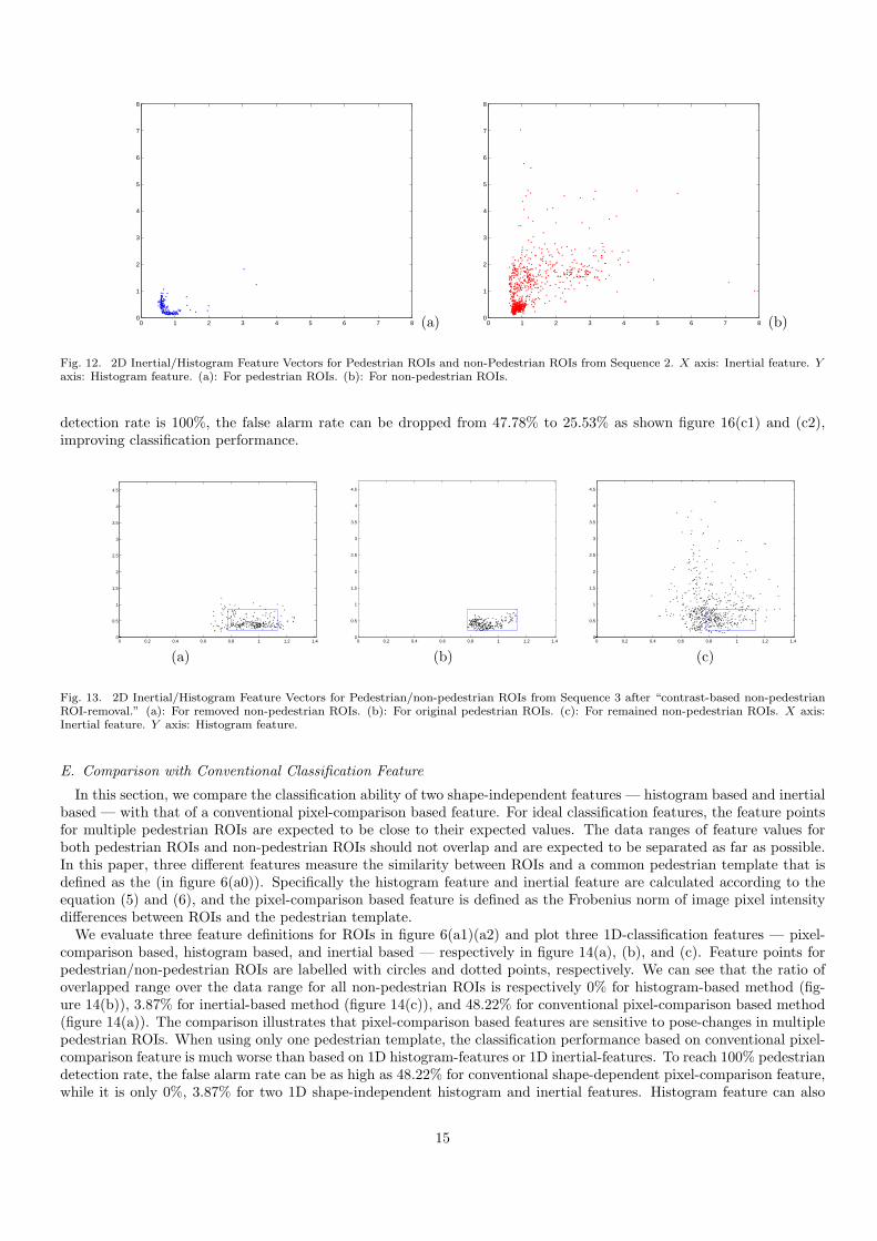
For 2D histogram/inertial-based classification method, the similarities between ROIs and one pedestrian template(in figure 6(a0)) are measured through 2D histogram/inertial feature vectors. The statistical distribution of 2D his-togram/inertial feature vectors for all ROIs from three sequences in figure 17(a1)(b1)(c1) (details in section IV, table I)are respectively presented in figure 11(a)(b), 12(a)(b), and figure 13(b)(c). Figures for both pedestrian ROIs and non-pedestrian ROIs in the same sequences are plotted with the same axis to demonstrate the distribution differences offeature vectors. We can see that 2D feature values for all pedestrian ROIs are similar and close to their expected value[1, 0] (X axis: inertial. Y axis: histogram.) as shown in figure 11(a), 12(a), and figure 13(b). Histogram/inertialfeature vectors for non-pedestrian ROIs are away from [1, 0] and much more diversified, as shown in figure 11(b), 12(b),and figure 13(c). (Non-pedestrian ROIs in figure 13(c) are after “contrast-based non-pedestrian ROI-removal.”) Thecomparison confirms that 2D histogram/inertial-based features are efficient classification feature vectors.

0 2 4 6 8 10 120

5

10

15

20

25

0 2 4 6 8 10 120

5

10

15

20

25

0 2 4 6 8 10 120.2

0.3

0.4

0.5

0.6

0.7

0.8

0.9

0 2 4 6 8 10 120.2

0.3

0.4

0.5

0.6

0.7

0.8

0.9

(a) (b) (c) (d)

Fig. 11. 2D Feature Vectors for Pedestrian ROIs and non-Pedestrian ROIs from Sequence 1. For (a)(b): 2D inertial/histogram featurevectors for pedestrian ROIs and non-pedestrian ROIs respectively. X axis: Inertial feature. Y axis: “Histogram Difference,” for ROIs andpedestrian template in figure 6(a0). For (c)(d): 2D inertial/pixel-comparison based feature vectors for pedestrian ROIs and non-pedestrianROIs respectively. X axis: Inertial feature. Y axis: “Image-Intensity-Difference” between ROIs and pedestrian template in figure 6(a0).In figure 11(a) and (b), histogram feature points for 19.64% of pedestrian ROIs and 16.13% of non-pedestrian ROIs overlap in their dataranges. In figure 11(c) and (d), pixel-comparison based feature points for all pedestrian ROIs and 85.74% of non-pedestrian ROIs overlapin their data ranges. The comparison between (a)(b) and (c)(d) shows the advantages of the histogram feature over the shape-dependentpixel-comparison based feature.

D.2 3D Histogram/Inertial/Contrast-based Classification

Our 3D histogram/inertial-feature/contrast-based classification algorithm first calculates ROI contrast-feature vec-tors for each ROI, then removes a few non-pedestrian ROIs based on two conditions mentioned in section III-C, andfinally identifies pedestrians among the rest of ROIs through 2D histogram/inertial based classification. An exampleof the process is shown in figure 10 and figure 13 for sequence 3 shown in figure 17(c1) (details in section IV, table I).After segmentation, there are total 248 pedestrian ROIs and 854 non-pedestrian ROIs whose contrast-feature vectors areplotted in figure 10. In the process of “contrast-based non-pedestrian ROI-removal,” 284 non-pedestrian ROIs lackingin clear vertical contrast are identified and removed. The inertial vs. histogram 2D feature vectors for 284 removednon-pedestrians, 248 segmented pedestrian ROIs and 570 remained non-pedestrian ROIs are respectively plotted infigure 13(a)(b)(c). The comparison between figure 13(a)(b) shows that 2D feature points for 76.76% of removed non-pedestrian ROIs are within the data range for pedestrian ROIs. The contrast-based feature helps to remove potentialambiguity using 2D histogram/inertial-based classification alone. Therefore, after “contrast-based non-pedestrian ROI-removal”, the percentage of segmented non-pedestrian ROIs, whose 2D feature vectors overlap with that of segmentedpedestrian ROIs in 2D feature space, has dropped from 47.78% to 25.53% (as shown in figure 13(b)(c)). Thus when

14

0 1 2 3 4 5 6 7 80

1

2

3

4

5

6

7

8

(a) 0 1 2 3 4 5 6 7 80

1

2

3

4

5

6

7

8

(b)

Fig. 12. 2D Inertial/Histogram Feature Vectors for Pedestrian ROIs and non-Pedestrian ROIs from Sequence 2. X axis: Inertial feature. Yaxis: Histogram feature. (a): For pedestrian ROIs. (b): For non-pedestrian ROIs.

detection rate is 100%, the false alarm rate can be dropped from 47.78% to 25.53% as shown figure 16(c1) and (c2),improving classification performance.

0 0.2 0.4 0.6 0.8 1 1.2 1.40

0.5

1

1.5

2

2.5

3

3.5

4

4.5

0 0.2 0.4 0.6 0.8 1 1.2 1.40

0.5

1

1.5

2

2.5

3

3.5

4

4.5

0 0.2 0.4 0.6 0.8 1 1.2 1.40

0.5

1

1.5

2

2.5

3

3.5

4

4.5

(a) (b) (c)

Fig. 13. 2D Inertial/Histogram Feature Vectors for Pedestrian/non-pedestrian ROIs from Sequence 3 after “contrast-based non-pedestrianROI-removal.” (a): For removed non-pedestrian ROIs. (b): For original pedestrian ROIs. (c): For remained non-pedestrian ROIs. X axis:Inertial feature. Y axis: Histogram feature.

E. Comparison with Conventional Classification Feature

In this section, we compare the classification ability of two shape-independent features — histogram based and inertialbased — with that of a conventional pixel-comparison based feature. For ideal classification features, the feature pointsfor multiple pedestrian ROIs are expected to be close to their expected values. The data ranges of feature values forboth pedestrian ROIs and non-pedestrian ROIs should not overlap and are expected to be separated as far as possible.In this paper, three different features measure the similarity between ROIs and a common pedestrian template that isdefined as the (in figure 6(a0)). Specifically the histogram feature and inertial feature are calculated according to theequation (5) and (6), and the pixel-comparison based feature is defined as the Frobenius norm of image pixel intensitydifferences between ROIs and the pedestrian template.

We evaluate three feature definitions for ROIs in figure 6(a1)(a2) and plot three 1D-classification features — pixel-comparison based, histogram based, and inertial based — respectively in figure 14(a), (b), and (c). Feature points forpedestrian/non-pedestrian ROIs are labelled with circles and dotted points, respectively. We can see that the ratio ofoverlapped range over the data range for all non-pedestrian ROIs is respectively 0% for histogram-based method (fig-ure 14(b)), 3.87% for inertial-based method (figure 14(c)), and 48.22% for conventional pixel-comparison based method(figure 14(a)). The comparison illustrates that pixel-comparison based features are sensitive to pose-changes in multiplepedestrian ROIs. When using only one pedestrian template, the classification performance based on conventional pixel-comparison feature is much worse than based on 1D histogram-features or 1D inertial-features. To reach 100% pedestriandetection rate, the false alarm rate can be as high as 48.22% for conventional shape-dependent pixel-comparison feature,while it is only 0%, 3.87% for two 1D shape-independent histogram and inertial features. Histogram feature can also

15

identify the second pedestrian ROI in figure 6(a1) that contains extra background region. Figure 14(d) plots 2D inertial(X axis) vs. histogram (Y axis) feature vectors for all ROIs. The comparison between figure 14(d) and figure 14(a)-(c)shows the advantages of 2D based histogram/inertial classification over each 1D classification.

To statistically demonstrate the above advantages, similar comparison is shown in figure 11 for a large set of ROIsfrom sequence 1 shown in figure 17(a1) (details in section IV, table I). Figure 11(a)(b) are inertial feature (X axis) vs.histogram feature (Y axis), and figure 11(c)(d) are inertial feature (X axis) vs. pixel-comparison based feature (Y axis).In the vertical axis of figure 11(a) and (b), histogram feature points for 19.64% of pedestrian ROIs and 16.13% of non-pedestrian ROIs overlap in their data ranges. In the vertical axis of figure 11(c) and (d), pixel-comparison based featurepoints for all pedestrian ROIs and 85.33% of non-pedestrian ROIs overlap. In 2D inertial vs. histogram space, the ratiosof overlapped range over the data range for all pedestrian ROIs and for all non-pedestrian ROIs are respectively 12.13%and 16.31%. As expected, the histogram features provide better classification performance than the shape-dependentpixel-comparison based feature. Classification based on both histogram and inertial further improve performance. Moreresults will be shown in the next section to demonstrate the advantages of multi-dimensional-classification as shown infigure16.

(a)

(b)

(c)

(d)

Fig. 14. Classification Ability Comparison. For (a)-(d): feature points of different definitions that measure the similarity between ROIs infigure 6(a1)(a2) and the default pedestrian template shown in figure 6(a0). Circles and dots respectively denote pedestrian ROIs and non-pedestrian ROIs. (a): Conventional 1D Pixel-Comparison based Feature. (b): 1D Histogram-based Feature. (c): 1D Inertial-based Feature.(d): 2D Histogram/Inertial Feature. For (a)-(c): Bottom/Top lines: data ranges for pedestrian/non-pedestrian ROIs. X axis: feature value.The Y axis is only used to separate two lines. The overlap percentage between them over non-pedestrian data range: 48.22%(a), 0%(b),3.87%(c). For (d): X axis: inertial value. Y axis: histogram difference value.

IV. Performance Evaluation

Up to now, we have presented our segmentation and classification algorithms. In real-world applications, bothbrightness-based and bodyline-based segmentation will be applied, and all segmented ROIs will be sent to multi-dimensional histogram-inertial-contrast-based classifiers for reliability. In this paper, for the purpose of performanceevaluation, we apply different combinations of segmentation/classification algorithms to detect pedestrians in three typ-ical scenarios: winter driving (Sequence 1, figure 17(a1)), summer suburban driving (Sequence 2, figure 17(b1)), andsummer urban driving (Sequence 3, figure 17(c1)). From sequence 1 to sequence 3, driving complexity increases. Forsequence 1 and 2, even the simplified version of our pedestrian detection (segmentation/classification) algorithm hasimproved the current detection performance as shown in figure 3, which demonstrates the potential and effectiveness ofour algorithms.

In this section we first introduce the basic information for the three sequences as summarized in table I. Then wepresent segmentation results in section IV-B) as summarized in table II, and classification results in section IV-C assummarized in table III. Pedestrian detection examples for three sequences are shown in figure 17(a), (b), and (c). Theinitial ROIs (after segmentation) and final detection results (after classification) are highlighted.

A. Test Sequences

The examples of pedestrian appearances for three sequences can be seen respectively in figure 6 (sequence 1) andfigure 7(a1)(a2) (sequence 2 and 3). All these video sequences were taken by Toyota R&D labs using a far-infrared

16

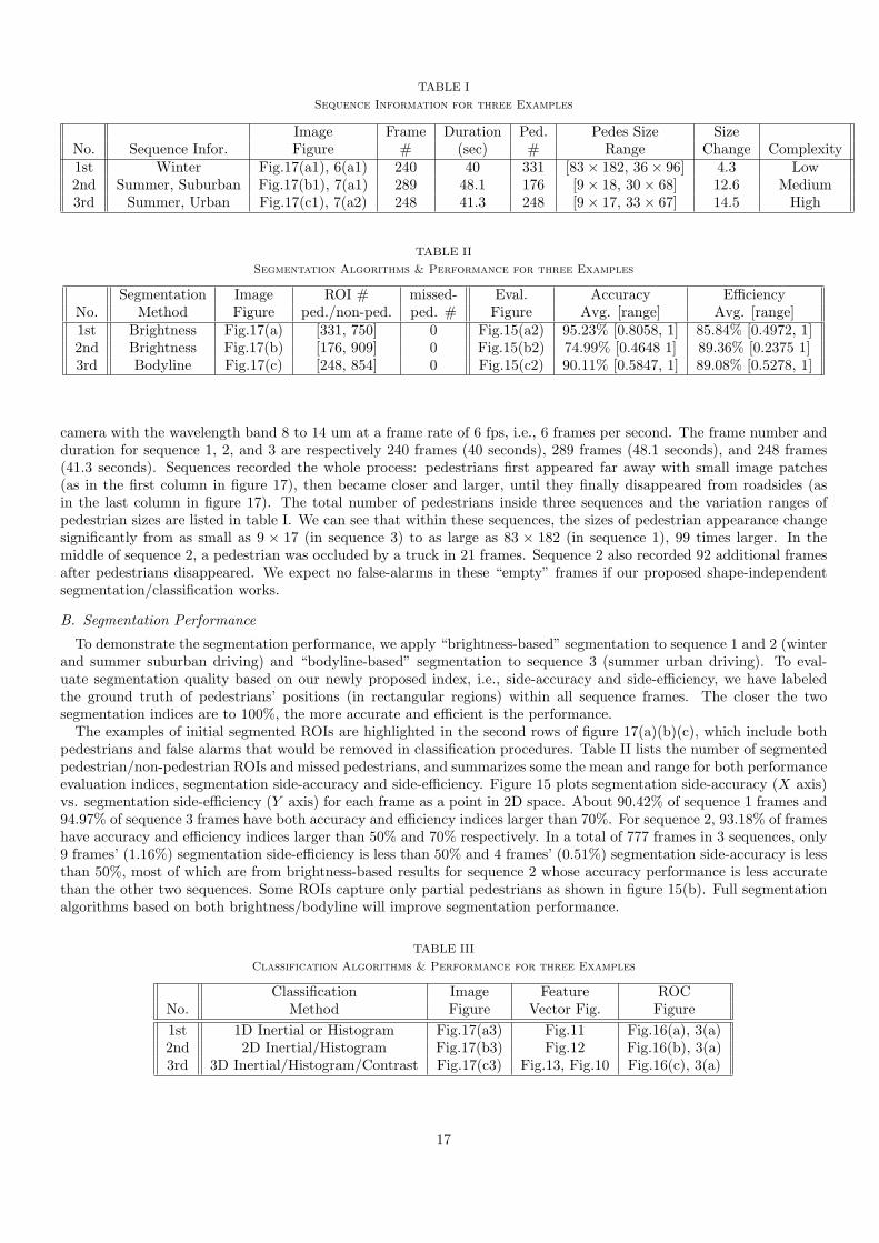
TABLE I

Sequence Information for three Examples

Image Frame Duration Ped. Pedes Size SizeNo. Sequence Infor. Figure # (sec) # Range Change Complexity1st Winter Fig.17(a1), 6(a1) 240 40 331 [83× 182, 36× 96] 4.3 Low2nd Summer, Suburban Fig.17(b1), 7(a1) 289 48.1 176 [9× 18, 30× 68] 12.6 Medium3rd Summer, Urban Fig.17(c1), 7(a2) 248 41.3 248 [9× 17, 33× 67] 14.5 High

TABLE II

Segmentation Algorithms & Performance for three Examples

Segmentation Image ROI # missed- Eval. Accuracy EfficiencyNo. Method Figure ped./non-ped. ped. # Figure Avg. [range] Avg. [range]1st Brightness Fig.17(a) [331, 750] 0 Fig.15(a2) 95.23% [0.8058, 1] 85.84% [0.4972, 1]2nd Brightness Fig.17(b) [176, 909] 0 Fig.15(b2) 74.99% [0.4648 1] 89.36% [0.2375 1]3rd Bodyline Fig.17(c) [248, 854] 0 Fig.15(c2) 90.11% [0.5847, 1] 89.08% [0.5278, 1]

camera with the wavelength band 8 to 14 um at a frame rate of 6 fps, i.e., 6 frames per second. The frame number andduration for sequence 1, 2, and 3 are respectively 240 frames (40 seconds), 289 frames (48.1 seconds), and 248 frames(41.3 seconds). Sequences recorded the whole process: pedestrians first appeared far away with small image patches(as in the first column in figure 17), then became closer and larger, until they finally disappeared from roadsides (asin the last column in figure 17). The total number of pedestrians inside three sequences and the variation ranges ofpedestrian sizes are listed in table I. We can see that within these sequences, the sizes of pedestrian appearance changesignificantly from as small as 9 × 17 (in sequence 3) to as large as 83 × 182 (in sequence 1), 99 times larger. In themiddle of sequence 2, a pedestrian was occluded by a truck in 21 frames. Sequence 2 also recorded 92 additional framesafter pedestrians disappeared. We expect no false-alarms in these “empty” frames if our proposed shape-independentsegmentation/classification works.

B. Segmentation Performance

To demonstrate the segmentation performance, we apply “brightness-based” segmentation to sequence 1 and 2 (winterand summer suburban driving) and “bodyline-based” segmentation to sequence 3 (summer urban driving). To eval-uate segmentation quality based on our newly proposed index, i.e., side-accuracy and side-efficiency, we have labeledthe ground truth of pedestrians’ positions (in rectangular regions) within all sequence frames. The closer the twosegmentation indices are to 100%, the more accurate and efficient is the performance.

The examples of initial segmented ROIs are highlighted in the second rows of figure 17(a)(b)(c), which include bothpedestrians and false alarms that would be removed in classification procedures. Table II lists the number of segmentedpedestrian/non-pedestrian ROIs and missed pedestrians, and summarizes some the mean and range for both performanceevaluation indices, segmentation side-accuracy and side-efficiency. Figure 15 plots segmentation side-accuracy (X axis)vs. segmentation side-efficiency (Y axis) for each frame as a point in 2D space. About 90.42% of sequence 1 frames and94.97% of sequence 3 frames have both accuracy and efficiency indices larger than 70%. For sequence 2, 93.18% of frameshave accuracy and efficiency indices larger than 50% and 70% respectively. In a total of 777 frames in 3 sequences, only9 frames’ (1.16%) segmentation side-efficiency is less than 50% and 4 frames’ (0.51%) segmentation side-accuracy is lessthan 50%, most of which are from brightness-based results for sequence 2 whose accuracy performance is less accuratethan the other two sequences. Some ROIs capture only partial pedestrians as shown in figure 15(b). Full segmentationalgorithms based on both brightness/bodyline will improve segmentation performance.

TABLE III

Classification Algorithms & Performance for three Examples

Classification Image Feature ROCNo. Method Figure Vector Fig. Figure1st 1D Inertial or Histogram Fig.17(a3) Fig.11 Fig.16(a), 3(a)2nd 2D Inertial/Histogram Fig.17(b3) Fig.12 Fig.16(b), 3(a)3rd 3D Inertial/Histogram/Contrast Fig.17(c3) Fig.13, Fig.10 Fig.16(c), 3(a)

17

0 0.1 0.2 0.3 0.4 0.5 0.6 0.7 0.8 0.9 10

0.1

0.2

0.3

0.4

0.5

0.6

0.7

0.8

0.9

1

0 0.1 0.2 0.3 0.4 0.5 0.6 0.7 0.8 0.9 10

0.1

0.2

0.3

0.4

0.5

0.6

0.7

0.8

0.9

1

0 0.1 0.2 0.3 0.4 0.5 0.6 0.7 0.8 0.9 10

0.1

0.2

0.3

0.4

0.5

0.6

0.7

0.8

0.9

1

Fig. 15. Segmentation Evaluation for 3 Sample Sequences. Detection Accuracy vs. Efficiency. X axis: frame segmentation side-accuracy. Yaxis: frame segmentation side-efficiency. (a): Sequence 1. (b): Sequence 2. (c): Sequence 3.

C. Classification Performance

The classification algorithms for three sequences are respectively 1D histogram-based, 2D histogram/inertial-based,and 3D histogram/inertial/contrast-based. For three sequences, their classification performance indices — ROC bound-ary as defined in I-A — are respectively plotted with solid lines in figure 16 (a), (b), and (c2). All ROC curves orROC boundaries are close to the ideal ROC boundary shown in figure 2(b), and present high detection rate and smallfalse-alarm rate.

The examples of classification results are highlighted in the third rows of figure 17(a)(b)(c), where some false alarmsare removed. Figure 3(a) compares the classification results of marked points in figure 16(a)(b)(c2), and other availablepublished results in different seasons by plotting their frame false-alarm/detection rate index points in 2D space. Forwinter driving, we mark ROI curve points in figure 16(a) whose false-alarm rate is similar to other published winterresult[18] and notice that our detection rate is higher.

For summer driving, we mark ROI curve points in figure 16(b)(c2) whose detection rates are similar to other publishedsummer results[12] and notice that our false-alarm rates are smaller. Figure 3(a) shows that our classification indexpoints are at the upper and left regions of other classification results and present higher detection rate with less falsealarm.

The performance of 1D histogram-based classification performance (figure 16(a)) is reliable for winter driving sequence1, which partially benefits from accurate segmentation performance as shown in figure 15. In general, 1D-feature-basedclassification performance is limited for summer driving as shown in figure 16(b) (sequence 2) and (c) (sequence 3)where dashed and dotted lines are respectively for 1D-histogram-based and 1D-inertial-based classification. It is becauseof more complex image property and more image “noise” for summer images. Besides, brightness-based segmentationaccuracy for summer suburban driving sequence 2 is relatively less accurate than for winter driving, which adds toclassification difficulties.

Fusing histogram-based and inertial-based classification substantially improves classification performance as shown bythe ROC-curve-comparison between solid lines (for 2D histogram/inertial-based classification) and dashed/dotted lines(for 1D histogram-based and 1D inertial-based classification) in figure 16(b) (sequence 2) and (c) (sequence 3). Final2D histogram/inertial classification performance for sequence 2 reflects its effectiveness for summer suburban driving.

The contrast classification feature helps to remove the ambiguity. Figure 16(c1) and figure 16(c2) respectively showthe different classification results before and after “contrast-based non-pedestrian ROI-removal.” The advantage of3D histogram/inertial/contrast-based classification over 2D histogram/inertial-based classification can be seen from thedifference between solid lines in figure 16(c1) and (c2). The comparison between dashed (or dotted) lines in figure 16(c1)and (c2) shows the advantage of 2D histogram/contrast-based (or 2D inertial/contrast-based) classification over 1Dhistogram (or 1D inertial) based classification. For three sequences, we only apply 3D histogram/inertial/contrast-basedclassification to the most complicated sequence 3 as shown in figure 16(c2) since 1D or 2D classification has alreadyprovided reliable results for the rest of sequences.

In sum, the segmentation performance illustrated in figure 15 shows that segmented pedestrian regions are relativelyaccurate and efficient. The classification performance illustrated in figure 16 show that most false alarms are removed.

18

(a) (b)

(c1) (c2)

Fig. 16. Classification Performance Evaluation for Three Sample Sequences. X axis: false alarm rate. Y axis: detection rate. (a): Sequence 1:ROC for histogram-based classification. (b): Sequence 2: Histogram/inertial-based classification. Dashed line: ROC for inertial-based classifi-cation. Dotted line: ROC for histogram-based classification results. Star points: Histogram/inertial-based classification result. (c1) Sequence3: ROC for histogram/inertial-based classification. Dashed line: ROC for inertial-based classification. Dotted line: ROC for histogram-basedclassification results. Star points: Histogram/inertial-based classification result. (c2) Sequence 3: ROC for histogram/inertial/contrast-basedclassification. Dashed line: ROC for inertial/contrast-based classification. Dotted line: ROC for histogram/contrast-based classificationresults. Star points: Histogram/inertial/contrast-based classification result.

V. Summary and Future work

This paper presents new methods for detecting pedestrians in far-infrared images in order to improve night drivingsafety. To reliably detect pedestrians with arbitrary poses, we introduce a new “Shape-Independent” detection methodthat stands in contrast to conventional shape-based detection methods to improve performance. In summary, there aretwo main contributions:

1. We propose an original “horizontal-first, vertical-second” segmentation scheme that first divides infrared imagesinto several vertical image stripes, and then searches for pedestrians only within these image stripes. The algorithm canautomatically estimate the size of pedestrian regions based on properties of the bright-pixel vertical-projection curvesand pedestrians’ horizontal contrast. Thus, we avoid brute-force searching over the entire images. Our algorithm haswide applicability, since it only assumes that there is some local contrast between the image of a pedestrian and itssurround and does not make other assumptions about the driving environment.

2. We have defined unique new shape-independent multi-dimensional classification features, specifically, histogram-,inertial-, and contrast-based features, and also demonstrated the similarities of these features among pedestrian imageregions with different poses, as well as the differences of these features between pedestrian and non-pedestrian ROIs. The“histogram variation curve” for all pedestrian regions resembles a Gaussian shape of zero mean, while the distributionof inertial-features resembles a Rayleigh distribution with expected value 1. Contrast-features — the ROI row-edgeindices, and the upper/lower row-edge indices — for pedestrian ROIs fall within specific data regions. In this way,pedestrians can be identified by comparing the similarity of these features derived from segmented ROIs with those ofa pedestrian template. Only one generic pedestrian template is needed. In contrast, traditional image pixel-comparisonbased classification is shape-dependent and so multiple pedestrian templates are necessary to deal with pedestrians indifferent poses.

On the whole, though the proposed pedestrian detection is by no means perfect for real world applications and we still

19

need to further improve the detection performance, it has made much progress considering the current research stages,and present encouraging results. Shape-independent features are more robust with respect to pedestrian pose-changesthan traditional shape-dependent features. Also, our segmentation and classification processes collaborate with oneanother. Initial horizontal segmentation and bodyline searching improves the segmentation accuracy and efficiency, andfewer segmentation errors lead to fewer classification errors. At the same time, the computational load is low becauseour segmentation process avoids brute-force searching over the whole image and the classification process avoids theneed for comparison with multiple pedestrian templates. The proposed new statistical features can be fused with othergeneral pedestrian detection features for multi-dimensional feature-based detection to further improve reliability andspeed.

References

[1] http://nncf.unl.edu/eldercare/info/seniordriving/nightdrive.html. Technical Report 6, Nebraska Highway Safety Program and theLincoln-Lancaster County Health Department, July 2001.

[2] C. Curio, J. Edelbrunner, T. Kalinke, C. Tzomakas, and W. von Seelen. Walking pedestrian recognition. IEEE Transactions on ITS,Vol. 1 No.3, pages 155–163, Sept. 2000.

[3] Cristobal Curio, Johann Edelbrunner, Thosmas Kalinke, Christos Tzomakas, and Werner Vonn Seelen. Walking pedestrian rocognition.IEEE Transactions on ITS, Vol. 1 No.3, pages 155–163, Sept. 2000.

[4] T. Darrell, G. Gordon, M. Harville, and J. Woodfill. Integrated person tracking using stereo, color, and pattern detection. CVPR,pages 601–609, 1998.

[5] D.M.Gavrila and J.Giebel. Shape-based pedestrian detection and tracking. Proc. of IEEE Intelligent Vehicles Symposium, 2002.

[6] Yajun Fang, Keiichi Yamada, Yoshiki Ninomiya, Berthold Horn, and Ichiro Masaki. Comparison between infrared-image-based andvisible-image-based approaches for pedestrian detection. Proceedings of the IEEE Intelligent Vehicles Symposium, pages 505–510, 2003.

[7] Yann Guilloux and Marie Bruyas. Aroto project: the benefit of infrared imagery for obstacle avoidance. Proc. of IEEE IntelligentVehicles Symposium, 2002.

[8] the United States Department of Transportation Intelligent Transportation Society of America. National intelligent transportationsystem program plan: A ten-year vision. Technical report, January 2002.

[9] M.Bertozzi, A.Broggi, A.Fascioli, and S.Nichele. Stereo vision-based vehicle detection. Proc. of IEEE Conf. on Intelligent TransportationSystem, pages 717–722, 1997.

[10] M.Bertozzi, A.Broggi, and etc. Vision-based pedestrian detection: will ants help. Proc. of IEEE Intelligent Vehicles Symposium, 2002.

[11] M.Bertozzi, A.Broggi, P.Grisleri, T.Graf, and M.Meinecke. Pedestrian detection and tracking with night vision. Proc. of IEEEIntelligent Vehicles Symposium, pages 662–667, 2003.

[12] Harsh Nanda and Larry Davis. Probabilistic template based pedestrian detection in infrared videos. Proc. of IEEE Intelligent VehiclesSymposium, 2002.

[13] M. Oren, C. Papageorgiou, P. Sinha, E. Osuna, and T. Poggio. Pedestrian detection using wavelet templates. CVPR, pages 193–199,1997.

[14] C. Papageorgiou and T. Poggio. Trainable pedestrian detection. Proc. of IEEE ICIP, pages 35–39, 1999.

[15] Chris Stauffer and W.E.L. Grimson. Adaptive background mixture methods for real-time tracking. IEEE Computer Society Conferenceon Computer Vision and Pattern Recognition, Vo.2, pages 246–252, 1999.

[16] Takayuki Tsuji, Hiroshi Hattori, Masahito Watanabe, and Nobuharu Nagaoka. Development of night-vision system. IEEE Transactionson ITS, Vol. 3 No.3, pages 203–209, Sept. 2002.

[17] C. Wohler, J.K.Aulaf, T.Portner, and U. Franke. A time delay neural network algorithm for real-time pedestrian detection. Proc. ofIEEE Intelligent Vehicles Symposium, pages 247–251, Oct. 1998.

[18] Fengliang Xu and Kikuo Fujimura. Pedestrian detection and tracking with night vision. Proc. of IEEE Intelligent Vehicles Symposium,2002.

[19] Liang Zhao and Charles E. Thorpe. Stereo and neural network-based pedestrian detection. IEEE Transactions on ITS, Vol. 1 No.3,pages 298–303, Sept. 2000.

20

(a1)

(a2)

(a3)(a) Sequence 1: brightness-based segmentation + Histogram-based classification

(b1)

(b2)

(b3)(b) Sequence 2: brightness-based segmentation + Histogram/Inertial-based classification

(c1)

(c2)

(c3)(c) Sequence 3: bodyline-based segmentation + Histogram/inertial/contrast-based classification

Fig. 17. Pedestrian detection performance for Sequence 1, 2, and 3. (a1)(b1)(c1): original images. (a2)(b2)(c2): Segmentation results.(a3)(b3)(c3): Classification results.

21