Active Learning with PartiallyAnnotated Sequence

(部分的アノテーションを用いた能動学習)

Dittaya WanvarieDepartment of Computational Intelligence and Systems Science

Tokyo Institute of Technology

A thesis submitted for the degree of

Doctor of Philosophy (Ph.D.)

September 2011

Abstract

This thesis presents an active learning framework for sequence labeling taskwith the confidence re-estimation. The framework can reduce the annota-tion cost from the whole corpus to a partial corpus, while achieving theclassifier with similar accuracy. Active learning consists of 3 main parts,the sampling, the annotation, and the re-training phases. The confidencere-estimation can be augmented in all phases. The re-estimation in activelearning reduces the annotation cost in terms of labeled tokens. The sim-plified sampling is also proposed to reduce the annotation cost in terms ofcomputational time.

Acknowledgements

First and foremost, I owe my deepest gratitude to Prof. Manabu Okumura,who gave me the first opportunity to pursue my study in this laboratory.From the start, he consistently give me valuable advices and total supportson my research.

I am also indebted to Assoc. Prof. Hiroya Takamura, who always havebrilliant ideas and excellent suggestions. It is an honor to me to have himas a co-advisor. I would like to thank Dr. Kritsada Sriphaew for his encour-agement, discussions and assistance in my work. This thesis could not havebeen accomplished without help from my colleagues at Okumura laboratory,especially the group of system administrators.

During years of study, I receive the financial support from the Thai gov-ernment through the Strategic Frontier Research Scholarship. Without thissupport, my opportunity to pursue this study might be difficult. Finally, Iwish to thank my family, friends, and the Thai community in Japan whoalways give me moral support through these years of study.

ii

Contents

List of Figures v

List of Tables vii

1 Introduction 1

2 Conditional Random Fields 92.1 Graphical Model . . . . . . . . . . . . . . . . . . . . . . . . . . . . . . . 92.2 Linear Chain Conditional Random Fields . . . . . . . . . . . . . . . . . 112.3 Conditional Random Fields for Partially Annotated Sequences . . . . . 13

3 Active Learning 173.1 Sampling Strategy . . . . . . . . . . . . . . . . . . . . . . . . . . . . . . 173.2 Informative Instances . . . . . . . . . . . . . . . . . . . . . . . . . . . . 18

3.2.1 Uncertainty in the Prediction . . . . . . . . . . . . . . . . . . . . 193.2.2 Query by Committee . . . . . . . . . . . . . . . . . . . . . . . . . 20

3.3 Initial Training Set . . . . . . . . . . . . . . . . . . . . . . . . . . . . . . 213.4 Stopping Criteria . . . . . . . . . . . . . . . . . . . . . . . . . . . . . . . 223.5 Active Learning for Sequence Labeling . . . . . . . . . . . . . . . . . . . 23

4 Related work 274.1 Selected Baselines . . . . . . . . . . . . . . . . . . . . . . . . . . . . . . 29

5 Proposed Framework 335.1 Confidence Re-estimation in the Annotation . . . . . . . . . . . . . . . . 355.2 Confidence Re-estimation in the Training . . . . . . . . . . . . . . . . . 365.3 Token Sampling Strategy . . . . . . . . . . . . . . . . . . . . . . . . . . 37

iii

CONTENTS

5.4 Simplified Sampling . . . . . . . . . . . . . . . . . . . . . . . . . . . . . 385.5 Stopping Criterion . . . . . . . . . . . . . . . . . . . . . . . . . . . . . . 39

6 Experiments 416.1 Data and Evaluation . . . . . . . . . . . . . . . . . . . . . . . . . . . . . 41

6.1.1 CoNLL2000 . . . . . . . . . . . . . . . . . . . . . . . . . . . . . . 416.1.2 CoNLL2003 . . . . . . . . . . . . . . . . . . . . . . . . . . . . . . 426.1.3 Evalutaion . . . . . . . . . . . . . . . . . . . . . . . . . . . . . . 44

6.2 Parameter Tuning . . . . . . . . . . . . . . . . . . . . . . . . . . . . . . 456.2.1 Initial Training Set . . . . . . . . . . . . . . . . . . . . . . . . . . 456.2.2 Sampling Size . . . . . . . . . . . . . . . . . . . . . . . . . . . . . 466.2.3 Confidence Threshold . . . . . . . . . . . . . . . . . . . . . . . . 47

6.3 Baseline Systems . . . . . . . . . . . . . . . . . . . . . . . . . . . . . . . 486.4 Confidence Re-estimation in the Annotation . . . . . . . . . . . . . . . . 516.5 Confidence Re-estimation in the Training . . . . . . . . . . . . . . . . . 546.6 Token Sampling . . . . . . . . . . . . . . . . . . . . . . . . . . . . . . . . 546.7 The Computational Time . . . . . . . . . . . . . . . . . . . . . . . . . . 556.8 The Simplified Sampling . . . . . . . . . . . . . . . . . . . . . . . . . . . 576.9 Final Result . . . . . . . . . . . . . . . . . . . . . . . . . . . . . . . . . . 59

7 Conclusion and Future Work 61

References 63

iv

List of Figures

1.1 Gene data . . . . . . . . . . . . . . . . . . . . . . . . . . . . . . . . . . . 2

1.2 Text data . . . . . . . . . . . . . . . . . . . . . . . . . . . . . . . . . . . 2

1.3 Named entity recognition . . . . . . . . . . . . . . . . . . . . . . . . . . 4

1.4 Dependencies among output labels . . . . . . . . . . . . . . . . . . . . . 4

1.5 A general pool-based active learning framework . . . . . . . . . . . . . . 6

2.1 A trigram relationship . . . . . . . . . . . . . . . . . . . . . . . . . . . . 9

2.2 Graphical model: A factor graph . . . . . . . . . . . . . . . . . . . . . . 10

2.3 Sequence model . . . . . . . . . . . . . . . . . . . . . . . . . . . . . . . . 11

2.4 α and β calculation . . . . . . . . . . . . . . . . . . . . . . . . . . . . . . 13

2.5 Marginalized label . . . . . . . . . . . . . . . . . . . . . . . . . . . . . . 14

2.6 A partially annotated sequence . . . . . . . . . . . . . . . . . . . . . . . 14

3.1 A general pool-based active learning framework for sequence labeling task 22

3.2 Sequence and token score . . . . . . . . . . . . . . . . . . . . . . . . . . 23

3.3 Partial sampling and partial anntoation . . . . . . . . . . . . . . . . . . 25

4.1 [Tomanek09] . . . . . . . . . . . . . . . . . . . . . . . . . . . . . . . . . 29

4.2 [Tsuboi08] . . . . . . . . . . . . . . . . . . . . . . . . . . . . . . . . . . . 30

4.3 [Neubig10] . . . . . . . . . . . . . . . . . . . . . . . . . . . . . . . . . . . 30

5.1 Marginal probability as the prediction confidence: The confidence thresh-old is set to 0.90. There are 3 label types, B, I, and O. The figure afterthe label is the output probability of each label. After a token is labeled,the probability of all tokens will change. . . . . . . . . . . . . . . . . . . 34

v

LIST OF FIGURES

5.2 Confidence re-estimation in the annotation. An annotator labels on to-ken in the sequence in each step ((b) to (e)). At the final iteration,low-informative tokens (in bold figures) are labeled by the model predic-tion. . . . . . . . . . . . . . . . . . . . . . . . . . . . . . . . . . . . . . . 35

5.3 Confidence re-estimation in the training. An annotator labels one tokenin the sequence in each step ((b) to (e)). No token is explicitly labeledby the model prediction. . . . . . . . . . . . . . . . . . . . . . . . . . . . 37

5.4 An example of simplified sampling . . . . . . . . . . . . . . . . . . . . . 39

6.1 All-phrase chunking task . . . . . . . . . . . . . . . . . . . . . . . . . . . 416.2 F1 on the systems trained of different initial sets. Lines represent the

number of labeled tokens. Points of the same color represent the CPUtime. . . . . . . . . . . . . . . . . . . . . . . . . . . . . . . . . . . . . . . 46

6.3 F1 of the systems with different sampling sizes. Lines represent thenumber of labeled tokens. Points of the same color represent the CPUtime. . . . . . . . . . . . . . . . . . . . . . . . . . . . . . . . . . . . . . . 47

6.4 F1 of the systems with different confidence threshold. Lines representthe number of labeled tokens. Points of the same color represent theCPU time. . . . . . . . . . . . . . . . . . . . . . . . . . . . . . . . . . . . 48

6.5 F1 comparison among baseline systems . . . . . . . . . . . . . . . . . . . 506.6 Training time comparison among baseline systems . . . . . . . . . . . . 506.7 Label changes after re-estimation in the annotation phase . . . . . . . . 526.8 F1 of the model with re-estimation in the annotation phase . . . . . . . 536.9 Errors in the training set with and without re-estimation . . . . . . . . 536.10 F1 of the model with and without the re-estimation in the training phase 556.11 F1 of the sequence sampling and the token sampling . . . . . . . . . . . 566.12 CPU time of the training on different corpus size . . . . . . . . . . . . . 576.13 Single-iteration CPU time of the all-phrase chunking and single-type

chunking tasks . . . . . . . . . . . . . . . . . . . . . . . . . . . . . . . . 586.14 Cumulative CPU time of the all-phrase chunking and single-type chunk-

ing tasks . . . . . . . . . . . . . . . . . . . . . . . . . . . . . . . . . . . . 58

vi

List of Tables

6.1 CoNLL2000 data; Number of sequences, tokens, chunk types and chunksof all-phrase. NP chunking is the simplified task on the same data set. . 42

6.2 CoNLL2003 data: Number of sequences, tokens, chunk types and chunksof English NER task. . . . . . . . . . . . . . . . . . . . . . . . . . . . . . 43

6.3 Word types and examples . . . . . . . . . . . . . . . . . . . . . . . . . . 436.4 Prediction confusion marix . . . . . . . . . . . . . . . . . . . . . . . . . 446.5 Comparison between baseline systems on NP chunking task. Boldface

figures are F1 which are not statistically different from the supervised F1. 496.6 Result of each system on CoNLL2000 and CoNLL2003. Boldface figures

indicate that the F1 is not significantly different from the supervised F1.Shaded cells show the main disadvantage of the systems. . . . . . . . . . 59

vii

LIST OF TABLES

viii

Chapter 1

Introduction

A sequence is an important structure in the real world. A gene in Figure 1.11 is anexample of a sequence structure in the biological domain. A gene is a subsequence ofDNA or RNA in a chromosome, which represents a genetic trait of a living organism.There are also relationships among some diseases, genes, and the medicine [28]. Thestudy of genes can lead to the invention of a new medicine to cure a disease.

A sentence in a human language is in the form of a word sequence. The researchon human languages is called Natural Language Processing (NLP), which is the mainfocus of this thesis. We can extract much information from a sequence of words suchas the intention of the speaker [25], the person name noted in a text document [19].

Figure 1.2 is an excerpt from the Naoto Kan page in Wikipedia2. We try to find allperson names and organization names in the text. Since a name can be either a singleword or a sequence of words, finding names is equivalent to labeling a word or a wordsequence which are names.

More specifically, assigning a label to each unit in a sequence is called annotation.However, annotating all data by hand is not practical. Although a small text passagemay contain hundreds of words, a newspaper, for example, contains several passagesand requires a large amount of human effort to scan through the data collection. Thenumber of human genes is not exactly known yet but the recent estimation is approxi-mately twenty thousand genes [12]. If an expert need to annotate all data every timethe new data is presented, the annotation cost will become intractable.

1http://upload.wikimedia.org/wikipedia/commons/0/07/Gene.png Retrieved on June 21, 2011.2http://en.wikipedia.org/wiki/Naoto_Kan#Career Retrieved on June 21, 2011.

1

1. INTRODUCTION

Figure 1.1: Gene data

Figure 1.2: Text data

2

Recently, we can train a machine expert to perform this annotation task instead ofa human expert. A machine which can predict the output of the given input is called aclassifier. Various branches of training algorithms are well studied in machine learningfields. Generally, the training algorithms are divided into the following three broadclasses:

• Supervised learning. A human gives the supervision to the machine by annotatingthe correct output of the given data. There are adjustable parameters in eachlearning algorithm. We try to adjust these parameters through the training tomake the machine correctly predict the output.

• Unsupervised learning. A machine can learn to predict the correct output froma raw data collection without any human supervision. Learning algorithms in aclass will induce the underlying information or structure from the observed inputdata. For example, a clustering algorithm will group a set of instances which aresimilar to each other.

• Semi-supervised learning. A human gives some supervision to a part of the train-ing collection. A machine can learn from both the annotated and unannotateddata.

This thesis is concerned with the semi-supervised learning approach. Since the sizeof data collection is still extremely large, human supervision is still costly even whenwe have to annotate the entire data collection only once to train the machine. Forexample, the Penn treebank contains almost 5 million English words. The part-of-speech annotation requires approximately 22 minutes per 1000 word annotation [32].If there is a single expert, annotating the entire treebank requires 180,000 hours. Thedifficulty of the annotation also depends on the task and the data set. The speed of thesyntactic tree annotation in the Penn treebank is approximately 400 words per hour.Since syntactic annotation is more complex than the part-of-speech annotation, thetime for the syntactic annotation is clearly longer than the time for the part-of-speechannotation.

Moreover, the accuracy of the machine also depends on the distribution of traininginstances in the data set. A classifier trained on a data set but tested on differentdata set usually achieves low-accuracy [34]. Even though the text collections are from

3

1. INTRODUCTION

..Mr. .Vinken .is .chairman .of .Elsevier .N.V. ., .the .Dutch .publishing .group ..

.B-PER .I-PER .O .O .O .B-ORG .I-ORG .O .O .B-MISC .O .O .O

.PERSON .ORG .MISC

Figure 1.3: Named entity recognition

..In .July .2003 ., .the .DPJ .and .the .Liberal .Party .led .by ....

.O .O .O .O .O .B-ORG .O .O .B-ORG .I-ORG .O .O ....

.ORG .ORG

.

Figure 1.4: Dependencies among output labels

the same languages, there are other differences such as writing styles or documenttopics, which will affect the accuracy of the classifier. The number of new data setsare countless. When a new data set is provided, we cannot avoid manual annotationof new data, but we will try to minimize the annotation cost from the entire data setto a part of data set.

We formulate the labeling task as a sequence labeling. The objective of sequencelabeling is similar to the other classification tasks, which is to find the output for thegiven input. A classifier is trained to predict the desired output of the given input.Figure 1.3 shows an example of the sequence labeling task in NLP, the named entityrecognition task. There are 3 types of named entities in this figure, PERSON, ORG,and MISC. Since some entities consist of several words, we introduce 2 label types foreach entity. the beginning word in the entity (B-chunk), and other words in the entity(I -chunk).

However, the sequence labeling task has a structured output which is constructedfrom several substructures with some dependencies among them. Figure 1.4 shows adependency between the output of DPJ and Liberal Party. The semantic rule of the

4

word and between these two words indicates that both words should have the sameoutput label. The structured output increases the number of possible output to beextremely large, in a very sparse output space. This sparse output space will decreasethe accuracy of the classifier. One solution to this problem is to factorize the structureand perform the classification on its substructure. However, the dependencies amongthe substructures make the factorization not be trivial. Although we can assume thatthere is no dependency among substructures, we will show in the experiment thatneglecting these dependencies leads to poor prediction accuracy.

The dependencies among the output labels of a sequence make the annotation moredifficult than the annotation of a non-structured instance. The following example is thepart-of-speech labeling task. Let us have a sentence “There is a trap.” which contains4 words:

1. There, which is either an adverb (here and there) or a pronoun.

2. is, which is a verb.

3. a, which is a determiner.

4. trap, which is either a noun or a verb.

We will find part-of-speech label of each word. If a word trap stands alone, it can beeither a noun or a verb. However, the part-of-speech of the word trap in this sentencedepends on the part-of-speech of its previous words, according to the syntactic rules.If we consider the whole structure as a single input, there are 4 possible outputs;

1. ADV V DET N.

2. ADV V DET V.

3. PRON V DET N.

4. PRON V DET V.

The number of possible outputs will substantially increase when the sentence is long.However, the frequency of each output is extremely low. In other words, the outputspace is extremely sparse. This sparseness of output labels in the training set willdecrease the accuracy of the classifier trained on this training set. We can reduce the

5

1. INTRODUCTION

..

.

.

.....

.Unlabeled pool.

.

.

.

.

.

.Training pool

..

...

.

.θ

.sampling

.update

Figure 1.5: A general pool-based active learning framework

sparseness of the output by factorizing the structure into substructures, and performthe prediction in substructure level, but keep the dependency among the substructuresin the consideration.

Active learning is a learning framework which can reduce the annotation cost fromthe entire training set to a part of the training set [14]. The hypothesis behind activelearning is that the informativeness of each instance in the training set is not equal. Theinformativeness of the instance is the contribution to the accuracy of the classifier ifthe instance is annotated, and added to the training set. Active learning is an iterativeframework which gradually selects informative instances from the entire data set andadds to the training pool as shown in Figure 1.5. In order to reduce the annotationcost, we need to select only the highly informative instances. Therefore, we can reducethe annotation cost but keep the high level of accuracy. The active learning frameworkis also applicable to the sequence labeling task. The informative instance can either bethe whole sequence [44] or a part of sequence [53]. This thesis adopted the predictionconfidence of a token as the informativeness score. When the prediction confidence ofa token is low, it indicates that the token may contain crucial information which is notpreviously known to the tagger. Hence, we define such a token to be informative.

6

The dependency among output substructures also affects the annotation. When atoken in a sequence is annotated, this label information will affect the prediction con-fidence of its neighboring tokens. In order to reduce the annotation cost of a sequence,we can incorporate this information propagation idea into the annotation task. Wecall the idea Confidence re-estimation. A general active learning framework is initiallyproposed to a simple classification task whose output is not a structure. Therefore, wecan incorporate the confidence re-estimation into the annotation of the substructure,the training of a classifier, also the sampling strategy.

This thesis proposes to incorporate the re-estimation of confidence in every step ofan active learning framework. Furthermore, we analyze several parameters of activelearning, which will affect the annotation cost. We also propose the efficient samplingstrategy, which can reduce the computational cost from the re-estimation of confidence.

The outline of this thesis begins with the machine learning method adopted inthis thesis, the conditional random fields (CRFs), followed by the description of ageneral active learning framework. Chapter 4 describes the research work related tothe proposed framework in this thesis. Chapter 5 introduces the implementation ofconfidence re-estimation idea in each step of the active learning framework, and theefficient sampling strategy. Chapter 6 presents the experiments and analysis of theresults. Finally, we conclude the contribution of this thesis and suggest the future workin the last chapter.

7

1. INTRODUCTION

8

Chapter 2

Conditional Random Fields

The objective of a supervised classification task is to train a classifier to predict thehuman supervised output from the given input. In a probabilistic model, we can rep-resent the input and output with random variables. Let x and y represent the inputand output, respectively. We can draw a graph representation of the relationship be-tween the input and output. Each vertex represents a random variable, while an edgeindicates that there is a relationship between vertices.

Because of the sparseness of the structured output, we reformulate the structuredoutput prediction to the substructure prediction. However, we still need to maintainthe dependency among the substructures. A graphical model naturally handles thisproblem by modeling the dependency with the vertex and edge representation. There-fore, we adopt the graphical model in this thesis.

2.1 Graphical Model

A graphical model is a probabilistic model for which a graph denotes the conditionalindependence structure between random variables [7]. This thesis employs a particular

..w1.w2 .w3

..trigram

Figure 2.1: A trigram relationship

9

2. CONDITIONAL RANDOM FIELDS

..π(v)

.. .v

. .p(v|π(v))

(a) Directed model

..yA

.. .xA

. .ΨA(xA, yA)

(b) Undirected model

Figure 2.2: Graphical model: A factor graph

type of the graphical model, a factor graph. A factor graph is a bipartite graph.There are 2 vertex types in a factor graph, the variable vertices and the factor vertices.The variable vertices are input and output vertices, while the factor vertices are therelationships or dependencies among the variables.

We factorize the entire graph G into a number of factors. Each factor consistsof a sub graph A whose variable vertices are bound together with one relationship.For example, a trigram relationship in Figure 2.1 requires 3 word vertices. A trigramrelationship is a factor vertex, while 3 word vertices are variable vertices.

In a factor graph, the score of each factor is independent of the other factors. Wecan calculate the probability of G by the product of factors:

p(x,y) = 1

Z

∏A

ΨA(xA,yA) , (2.1)

where Ψ is a factor function spanned on a sub graph A. The constant Z is the normal-ization function:

Z =∑x,y

∏A

ΨA(xA,yA) . (2.2)

Figure 2.2 shows 2 types of a factor graph, the directed model and the undirectedmodel. Variables vertices are in circle shapes while factor vertices are in square shapes.The difference between these models is the dependence assumption behind the factorscore. A directed model is also known as a Bayesian network [22], which is based onthe joint probability, p(y,x) = p(y|x)p(x). A directed model is factorized to be

p(x,y) =∏v∈V

p(v|π(v)) , (2.3)

where π(v) is the parent of a vertex v in the graph G.

10

2.2 Linear Chain Conditional Random Fields

..xt−2 .xt−1 .xt .xt+1 .xt+2

.yt−2 .yt−1 .yt .yt+1 .yt+2

. .ss(xt|yt)

.

.s t(y t|y t−

1)

(a) Directed model

..xt−2 .xt−1 .xt .xt+1 .xt+2

.yt−2 .yt−1 .yt .yt+1 .yt+2

. .ss(xt, yt)

.

.s t(y t−1, y t

)

(b) Undirected model

Figure 2.3: Sequence model

On the other hand, an undirected model is based on the conditional probability,p(y,x) = p(y|x). An undirected model is factorized to be

p(x,y) =∏v∈V

p(v, π(v)) . (2.4)

We can adopt the graphical model on a classification task. For a single outputclassification, the directed version of the probabilistic model can be described in theform

p(x, y) = p(y)∏A

p(xA|y), (2.5)

which is a naive Bayes classifier [20]. An example of the undirected graphical versionis a logistic regression classifier, which is in the following form:

p(y|x) = 1

Z(x)e∑

A φA(xA,y) . (2.6)

2.2 Linear Chain Conditional Random Fields

A basic classification only has a single output y. In a structured output problem,the output is a set of labels with some dependencies among them. For a sequence

11

2. CONDITIONAL RANDOM FIELDS

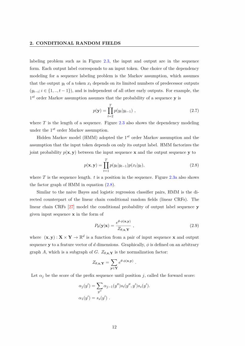
labeling problem such as in Figure 2.3, the input and output are in the sequenceform. Each output label corresponds to an input token. One choice of the dependencymodeling for a sequence labeling problem is the Markov assumption, which assumesthat the output yt of a token xt depends on its limited numbers of predecessor outputs(yt−i; i ∈ {1, .., t− 1}), and is independent of all other early outputs. For example, the1st order Markov assumption assumes that the probability of a sequence y is

p(y) =T∏t=2

p(yt|yt−1) , (2.7)

where T is the length of a sequence. Figure 2.3 also shows the dependency modelingunder the 1st order Markov assumption.

Hidden Markov model (HMM) adopted the 1st order Markov assumption and theassumption that the input token depends on only its output label. HMM factorizes thejoint probability p(x,y) between the input sequence x and the output sequence y to

p(x,y) =T∏t=1

p(yt|yt−1)p(xt|yt), (2.8)

where T is the sequence length. t is a position in the sequence. Figure 2.3a also showsthe factor graph of HMM in equation (2.8).

Similar to the naive Bayes and logistic regression classifier pairs, HMM is the di-rected counterpart of the linear chain conditional random fields (linear CRFs). Thelinear chain CRFs [27] model the conditional probability of output label sequence ygiven input sequence x in the form of

Pθ(y|x) =eθ·φ(x,y)

Zθ,x,Y, (2.9)

where �(x,y) : X×Y → Rd is a function from a pair of input sequence x and outputsequence y to a feature vector of d dimensions. Graphically, φ is defined on an arbitrarygraph A, which is a subgraph of G. Zθ,x,Y is the normalization factor:

Zθ,x,Y =∑y∈Y

eθ·φ(x,y) .

Let αj be the score of the prefix sequence until position j, called the forward score:

αj(y′) =

∑y′′

αj−1(y′′)st(y

′′, y′)ss(y′).

α1(y′) = ss(y

′) .

12

2.3 Conditional Random Fields for Partially Annotated Sequences

.. . .... . .j . .... ..ps(y′)

.pt(y′′, y′) .pt(y′, y′′).αj(y

′)

.βj(y′)

Figure 2.4: α and β calculation

Let βj be the score of the suffix sequence from position j, called the backward score:

βj(y′) =

∑y′′

st(y′, y′′)ss(y

′′)βj+1(y′′).

βT (y′) = 1 .

α and β calculation are shown in Figure 2.4. st(y′, y′′) is the transition score from label

y′ to label y′′. ss(y′) is the output score of label y′. We can efficiently compute Zθ,x,Y

byZθ,x,Y =

∑y′∈Y1

α1(y′) · β1(y′) ,

where Y1 is all possible labels of y1.θ ∈ Rd is a vector of model parameters. For a set of N training sequences

{(x(i),y(i))}, the learning process will maximize the following log likelihood function:

LL(θ) =N∑

n=1

ln(Pθ(y(n)|x(n))) . (2.10)

We can apply standard optimization techniques such as L-BFGS in [31] or SGD in [58],to the objective function in equation (2.10).

2.3 Conditional Random Fields for Partially AnnotatedSequences

The maximization of the objective function in equation (2.10) requires all tokens inthe input sequence to be labeled since some factors depend on the output labels. If asequence is partially labeled, we will not be able to calculate the score of those factors.

13

2. CONDITIONAL RANDOM FIELDS

..xt

.?

.

.

..y′ : p(yt = y′)ss(xt, y′)

..y′′ : p(yt = y′′)ss(xt, y′′)

..y′′′ : p(yt = y′′′)ss(xt, y′′′)

..∑

y p(yt = y) = 1

Figure 2.5: Marginalized label

..xt−2 .xt−1 .xt .xt+1 .xt+2

.yt−2 .yt−1 .y′′

.y′

.y′′′

.yt+1 .yt+2

.L = ((xt−2, yt−2), (xt−1, yt−1), (xt), (xt, xt+1, yt+1), (xt+2, yt+2))

Figure 2.6: A partially annotated sequence

One solution to this problem is to estimate the output label of all unlabeled tokensusing the marginalized outputs [5; 56]. Figure 2.5 shows the marginalized labels of thetoken xt. There are 3 possible labels, y′, y′′, and y′′′. Each output has a marginalizedprobability p(y′), p(y′′), and p(y′′′), respectively. We assign all possible output labelswith the corresponding marginal probability to xt.

Given a partially labeled sequence or ambiguously labeled sequence L, let YL bethe set of all possible output sequences consistent with L. For example, Figure 2.6consists of 5 input tokens, xt−2 to xt+2. All tokens except xt have a single output label.xt has 3 possible output labels, y′, y′′, and y′′′. Hence, YL consists of 3 sequence pairs:

• (x, (yt−2, yt−1, y′, yt+1, yt+2))

• (x, (yt−2, yt−1, y′, yt+1, yt+2))

• (x, (yt−2, yt−1, y′, yt+1, yt+2)).

We can estimate the probability of YL given x by

Pθ(YL|x) =∑

y∈YL

Pθ(y|x) . (2.11)

14

2.3 Conditional Random Fields for Partially Annotated Sequences

Using equation (2.11), the log likelihood in equation (2.10) is modified to

LL(θ) =

N∑n=1

lnPθ(YL(n) |x(n))

=

N∑n=1

(ln∑

y∈YL(n)

eθ·φ(x(n),y)∑

y′∈Y eθ·φ(x(n),y′))

=

N∑n=1

(ln∑

y∈YL(n)

eθ·φ(x(n),y) − ln

∑y′∈Y

eθ·φ(x(n),y′))

=

N∑n=1

(lnZθ,x(n),YL(n)− lnZθ,x(n),Y) . (2.12)

x(n) and L(n) are nth input sequence and a set of all possible output sequences,respectively. Zθ,x(n),YL(n)

can be computed by the forward-backward algorithm similarto the one used for Zθ,x,Y. We then apply the standard optimization techniques toequation (2.12) as done in equation (2.10).

15

2. CONDITIONAL RANDOM FIELDS

16

Chapter 3

Active Learning

Active learning is useful when manual labeling is costly. For example, labeling a part-of-speech of a word requires an expert [40]. In contrast, active learning may not bebeneficial for easy labeling task such as image classification through World Wide Web[48] or labeling through a computer game [60].

Active learning is an interactive learning which selectively chooses training instancesfrom the entire training set. In contrast to the passive learning, the selective samplingof active learning can reduce the annotation cost in terms of labeled instances andachieve high accuracy with the compensation of the training time.

3.1 Sampling Strategy

An early active learning approach is the membership query synthesis. A machine willask an annotator to label the selected unlabeled instance and the synthesized instance[3]. This approach is not practical in many real world applications because human an-notators have difficulties labeling the synthesized instance. More recent approaches arefallen in 2 categories, the stream-based selective sampling and the pool-based samplingstrategies. Both approaches ask an annotator to label the real data.

Stream-based sampling assumes that the training instance is given one by one to thelearning system, and will decide whether or not the given instance has to be labeled [14;16]. On the other hand, the pool-based active learning will directly select the traininginstances from the training pool [29]. The decision in stream-based sampling, and the

17

3. ACTIVE LEARNING

Algorithm 1 Active learning framework1: St : {(x,y)} is a set of all training sequences at iteration t

2: Ssel is a set of informative instances3: curmodel← train(S1) {Initial training}4: repeat5: Ssel ← Q(curmodel, St) {Sampling q instances}6: for x ∈ Ssel do7: St+1 ← St ∪ update(St, label(x)) {Annotation}8: end for9: curmodel← train(St+1) {Training}

10: until stopping criterion is satisfied

selection in pool-based sampling are based on the informativeness of the instance. Thisthesis is concerned with the pool-based sampling strategy.

Pool-based sampling active learning framework is roughly divided into 3 phases,the sampling of informative instances, the annotation, and the re-training phases, asshown in Algorithm 1. The framework starts from a small initial labeled set. In eachiteration, a model is trained using the current labeled set and is used to sample acollection of informative instances. An annotator is then asked to provide labels to theselected instances. Newly labeled data is added to the training set. The sampling andannotation are repeated until the stopping criterion is satisfied.

3.2 Informative Instances

An informative instance is an instance which can contribute to the desired result suchas high accuracy, if it is annotated and added to the training set. The key idea ofactive learning is that some instances in the training data are more informative thatthe others. Active learning will choose only informative instances for labeling; hencereducing the annotation cost from the entire training set.

The definition of the informativeness based on the contribution to the desired resultis hard to measure. Instead, we approximate the contribution by other measurements.

Let φ be the informativeness scoring function. This section provides two generalscoring functions which are widely used in active learning, the uncertainty score and

18

3.2 Informative Instances

the disagreement-among-committee score.

3.2.1 Uncertainty in the Prediction

The most popular informativeness measurement is the uncertainty of the prediction[44]. Given a single classifier, the classifier can predict output of an instance with somelevel of confidence. For a probabilistic model such as conditional random fields, theprediction confidence is in the form of output probability [15; 53]. For an input instancex, its informativeness in a probabilistic model is

φ(x) = 1− P (y∗|x) , (3.1)

where y∗ is the output label with the highest probability. When the output probabilityis high, it states that the model are confident in the prediction.

For a non-probabilistic model, we may obtain the probabilistic confidence by apply-ing the sigmoid function [37]. For example, a maximum margin classifier can predictthe output using the margin from the separating hyperplane. The margin score itself isa real value. Although we can normalize the margin score using the sigmoid function,the margin itself can be the prediction confidence [10; 41; 43; 55]. Let f(x, y) be thepredicted margin. The informativeness score of x is

φ(x) = −|f(x, y∗)| . (3.2)

When the absolute margin is large, it states that the model prediction is reliable.Apart from the uncertainty of the candidate with the highest prediction confidence,

the difference of confidence among the predictions is another measurement of uncer-tainty [9; 62]. We assume that a token will have a single output. For example, in thecase of a probabilistic model, the informativeness based on the confidence difference is

φ(x) = −(maxy′∈Y

P (y′|x)− maxy′′∈Y ;y′′ 6=y′

P (y′′|x)) , (3.3)

where y′ and y′′ are output labels in the set of all labels Y . When the difference betweenthe prediction confidence is small, it indicates that the classifier cannot distinguish thebest output from the other candidates. That instance will be highly informative.

Entropy of the prediction confidence is another measurement of uncertainty [46].The informativeness score based on the entropy is defined as

φ(x) =∑y′∈Y

P (y′|x) · log(P (y′|x)) . (3.4)

19

3. ACTIVE LEARNING

Low entropy represents the status that the classification is certain.High prediction confidence or low uncertainty result implies that training corpus

contains enough information for the classifier to distinguish the predicted output fromthe other outputs. Hence, an instance with high-prediction confidence is uninformativeand is not required to be annotated. On the other hand, when the prediction confidenceis low, it indicates that the training corpus lacks information to predict the output ofthe given input. An annotator should provide such information to the machine byannotating the instance. Therefore, such instances are informative.

3.2.2 Query by Committee

Instead of using a single classifier in the sampling strategy, we can use several classifierswith different hypotheses and evaluate the agreement among the prediction of classifiers[45]. There are two steps in the query by committee framework, the committee selectionand the agreement measurement.

A single classifier is based on a single training set and single hypothesis. When acommittee or a set of classifiers are necessary, we should either create several trainingsets or hypotheses. For the training set creation, we can randomly sample instancesto make several subsets of the entire training set. Then, we can train a classifier or acommittee on each subset. This method is called query by bagging [1]. For the creationof hypotheses, we can randomly set the model parameters according to some posteriordistributions P (θ|L). For example, McCallum and Nigam sampled the naive Bayesparameters from a Dirichlet distribution [33]. Dagan and Engelson sampled HMMparameters from a normal distribution [16].

For the agreement measurement, Dagan and Engelson proposed the voting entropywhich can measure the agreement among the prediction of the committee [16]. Sup-posing that there are C committee members, the voting entropy of the predicted labelsis

φ(x) = −∑y′∈Y

V (y′, x)

|C|log V (y′, x)

|C|, (3.5)

where V (y′, x) denotes the number of committee members that predict the output ofx to be y′. High entropy is interpreted as low agreement in the prediction. Thus, suchinstances are highly informative.

20

3.3 Initial Training Set

McCallum and Nigam proposed to measure the similarity between the prediction ofcommittee members and the average prediction of all committees using the Kullback-Liebler (KL) divergence [33]. If the probability of the prediction of a committee memberis Pc(y|x) and the average probability is

Pavg(y|x) =1

C

∑c

Pc(y|x), (3.6)

the KL divergence between these probability distributions is

D(Pc(y|x)||Pavg(y|x)) =∑y′∈Y

Pc(y′|x) log Pc(y

′|x)Pavg(y′|x)

. (3.7)

An instance with large divergence indicates that there is high disagreement among thepredictions. Therefore, the informativeness based on the KL divergence is

φ(x) =1

C

∑c

D(Pc(y|x)||Pavg(y|x)) . (3.8)

3.3 Initial Training Set

A typical initial set may start from a collection of random instances. However, iterativemethods are sensitive to the initial set, especially in the case of sparse data [24]. Areasonable initial set usually leads to convergence with less annotation cost.

A popular idea is to increase the coverage of the initial set as much as possible.Clustering-based methods are one of the famous selection strategies [24]. A represen-tative instance of each cluster is selected for the initial set. Therefore, the initial setwill have high coverage of the entire training set. The commonly used clustering algo-rithm is k-Means and its variations [24; 64]. Hu et al. proposed further-first-traversal,agglomerative hierarchical clustering, and affinity propagation clustering, which are de-terministic algorithms, for the initial set selection of active learning [23]. They havepointed out that the k-Means and its variations are non-deterministic approaches, andare inconsistent. The deterministic approaches are more stable and can guarantee thesame performance on every run.

In a structured output prediction problem, a large instance is supposed to containmore information than a small instance. Thereofre, a simple hueristic such as alwayschoosing large instances is also effective [44].

21

3. ACTIVE LEARNING

.

.

..x1 ..: ..w1 ..w2 ..w3 .....

..x2 ..: ..w1 ..w2 ..w3 .....

..x3 ..: ..w1 ..w2 ..w3 .....

. .....

.Unlabeled pool

.

..yi0 ..: ..l10 ..l2 ..... ..lT10

..xi0 ..: ..x10 ..x2 ..... ..xT10

..yi1 ..: ..l11 ..l2 ..... ..lT11

..xi1 ..: ..x11 ..x2 ..... ..xT11

.Training pool

.

..y1 ..: ..l1 ..l2 ..l3 ..... ..lT1

..x1 ..: ..w1 ..w2 ..w3 ..... ..wT1.

..y3 ..: ..l1 ..l2 ..l3 ..... ..lT3

..x3 ..: ..w1 ..w2 ..w3 ..... ..wT3

.

..y1 ..: ..l1 ..l2 ..... ..lT1

..x1 ..: ..x1 ..x2 ..... ..xT1

..y3 ..: ..l1 ..l2 ..... ..lT3

..x3 ..: ..x1 ..x2 ..... ..xT3

.θ

.sampling

.update

Figure 3.1: A general pool-based active learning framework for sequence labeling task

3.4 Stopping Criteria

An ideal stopping criteria is to finish with the highest accuracy, with the lowest anno-

tation cost. In other words, the annotator should not add more annotated instances if

those instances will not increase the accuracy. However, we do not know the accuracy

of the system in advance.

We may limit the percentage of data to be annotated, or number of the iterations

as a stopping criterion. The appropriate number depends on the task [59]. Another

stopping criterion is to use the development set to evaluate the accuracy of the classifier

[30]. However, this method requires an evaluation set to be annotated beforehand.

Vlachos proposed to evaluate the stopping criterion on an evaluation set, but they

did not evaluate the classifier using the accuracy. Instead, they use the prediction con-

fidence which does not require the annotated data [59]. We can also set the confidence

threshold to be the stopping criterion, and stop when there is no informative instance

according to the threshold [43].

22

3.5 Active Learning for Sequence Labeling.

...y1 ..: ..l1 ..l2 ..l3 ..... ..lT1

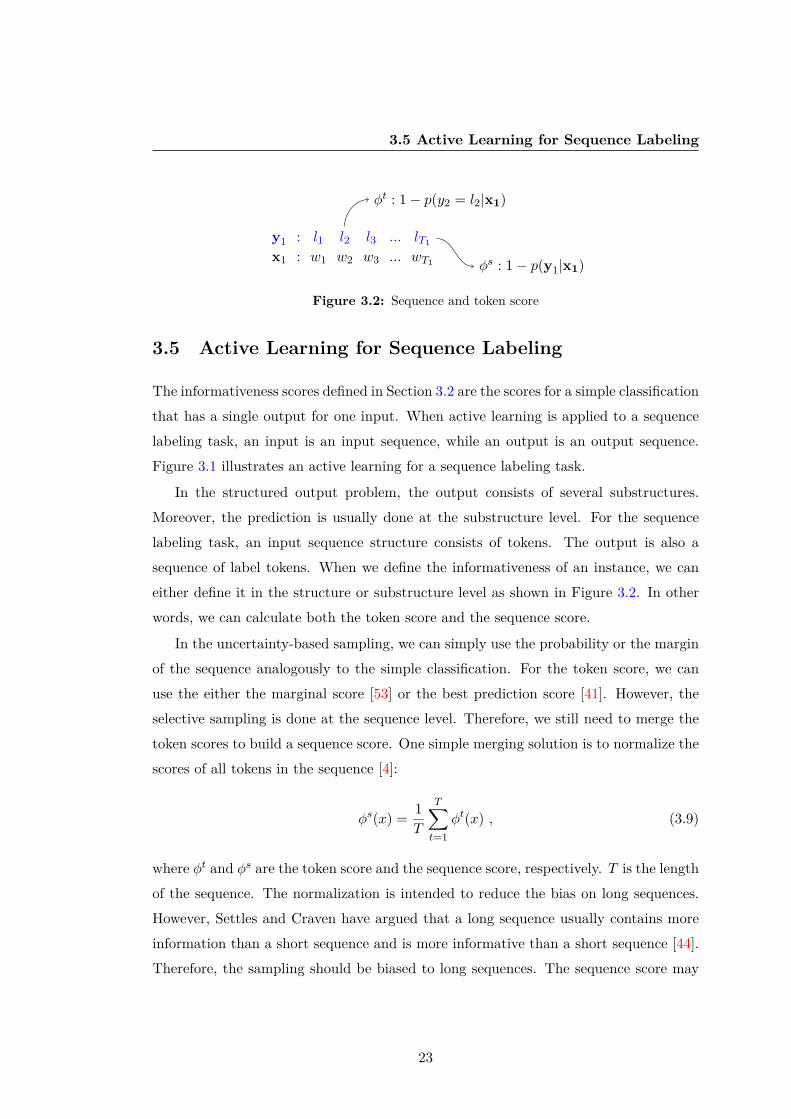
..x1 ..: ..w1 ..w2 ..w3 ..... ..wT1 .φs : 1− p(y1|x1)

.φt : 1− p(y2 = l2|x1)

Figure 3.2: Sequence and token score

3.5 Active Learning for Sequence Labeling

The informativeness scores defined in Section 3.2 are the scores for a simple classificationthat has a single output for one input. When active learning is applied to a sequencelabeling task, an input is an input sequence, while an output is an output sequence.Figure 3.1 illustrates an active learning for a sequence labeling task.

In the structured output problem, the output consists of several substructures.Moreover, the prediction is usually done at the substructure level. For the sequencelabeling task, an input sequence structure consists of tokens. The output is also asequence of label tokens. When we define the informativeness of an instance, we caneither define it in the structure or substructure level as shown in Figure 3.2. In otherwords, we can calculate both the token score and the sequence score.

In the uncertainty-based sampling, we can simply use the probability or the marginof the sequence analogously to the simple classification. For the token score, we canuse the either the marginal score [53] or the best prediction score [41]. However, theselective sampling is done at the sequence level. Therefore, we still need to merge thetoken scores to build a sequence score. One simple merging solution is to normalize thescores of all tokens in the sequence [4]:

φs(x) =1

T

T∑t=1

φt(x) , (3.9)

where φt and φs are the token score and the sequence score, respectively. T is the lengthof the sequence. The normalization is intended to reduce the bias on long sequences.However, Settles and Craven have argued that a long sequence usually contains moreinformation than a short sequence and is more informative than a short sequence [44].Therefore, the sampling should be biased to long sequences. The sequence score may

23

3. ACTIVE LEARNING

not have to be normalized by the sequence length:

φs(x) =

T∑t=1

φt(x) . (3.10)

For the label entropy in the uncertainty-based sampling, the straightforward calcu-lation will be

φs(x) = −∑y′

P (y′|x) logP (y′|x) . (3.11)

Since the summing over all possible y is intractable, Kim et al. proposed an approxi-mation of the calculation using the N -best output [26]:

φs(x) = −∑

y′∈NP (y′|x) logP (y′|x) , (3.12)

where N is the set of N best predictions.Similarly, the sequence voting entropy and the sequence KL divergence of the query

by committee strategy are also approximated using the N c-best output. N c is theunion of N -best outputs from all committee members. The sequence entropy becomes

φ(x) = −∑

y′∈Nc

V (y′,x)|C|

log V (y′,x)|C|

. (3.13)

The KL divergence is slightly changed to

D(Pc(y|x)||Pavg(y|x)) =∑

y′∈Nc

Pc(y′|x) log Pc(y′|x)Pavg(y′|x) . (3.14)

Since a structure consists of several substructures, the sampling and annotation canalso be done in the substructure level as illustrated in Figure 3.3. In the token anno-tation framework, only the informative tokens will be manually annotated. The othertokens can be labeled by the model estimation [53; 56]. In the substructure sampling,the entire structure is provided to an annotator because the context is important inthe annotation. However, an annotator needs to label only the specified substructure.Sassano and Kurohashi proposed to sample a chunk rather than a sentence in Japanesedependency parsing task [42]. Morevoer, Druck et al. proposed the sampling and theannotation of the features instead of the output label [18].

24

3.5 Active Learning for Sequence Labeling

.

.

..x1 ..: ..w1 ..w2 ..w3 .....

..x2 ..: ..w1 ..w2 ..w3 .....

..x3 ..: ..w1 ..w2 ..w3 .....

. .....

.Unlabeled pool

.

..yi0 ..: ..l10 ..l2 ..... ..lT10

..xi0 ..: ..x10 ..x2 ..... ..xT10

..yi1 ..: ..l11 ..l2 ..... ..lT11

..xi1 ..: ..x11 ..x2 ..... ..xT11

.Training pool

.

..y1 ..: . ..l2 ..l3 ..... .

..x1 ..: ..w1 ..w2 ..w3 ..... ..wT1.

..y3 ..: ..l1 . ..l3 ..... .

..x3 ..: ..w1 ..w2 ..w3 ..... ..wT3

.Manual annotation

.

..y1 ..: . ..l2 ..... .

..x1 ..: ..x1 ..x2 ..... ..xT1

..y3 ..: ..l1 . ..... .

..x3 ..: ..x1 ..x2 ..... ..xT3

.θ

.sampling

.update

Figure 3.3: Partial sampling and partial anntoation

25

3. ACTIVE LEARNING

26

Chapter 4

Related work

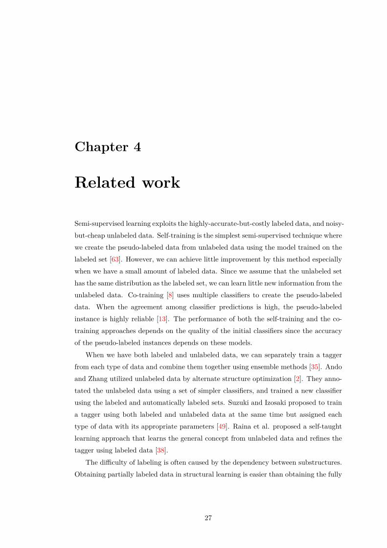
Semi-supervised learning exploits the highly-accurate-but-costly labeled data, and noisy-but-cheap unlabeled data. Self-training is the simplest semi-supervised technique wherewe create the pseudo-labeled data from unlabeled data using the model trained on thelabeled set [63]. However, we can achieve little improvement by this method especiallywhen we have a small amount of labeled data. Since we assume that the unlabeled sethas the same distribution as the labeled set, we can learn little new information from theunlabeled data. Co-training [8] uses multiple classifiers to create the pseudo-labeleddata. When the agreement among classifier predictions is high, the pseudo-labeledinstance is highly reliable [13]. The performance of both the self-training and the co-training approaches depends on the quality of the initial classifiers since the accuracyof the pseudo-labeled instances depends on these models.

When we have both labeled and unlabeled data, we can separately train a taggerfrom each type of data and combine them together using ensemble methods [35]. Andoand Zhang utilized unlabeled data by alternate structure optimization [2]. They anno-tated the unlabeled data using a set of simpler classifiers, and trained a new classifierusing the labeled and automatically labeled sets. Suzuki and Izosaki proposed to traina tagger using both labeled and unlabeled data at the same time but assigned eachtype of data with its appropriate parameters [49]. Raina et al. proposed a self-taughtlearning approach that learns the general concept from unlabeled data and refines thetagger using labeled data [38].

The difficulty of labeling is often caused by the dependency between substructures.Obtaining partially labeled data in structural learning is easier than obtaining the fully

27

4. RELATED WORK

labeled data in some tasks. In the machine-aided corpus annotation, the annotatorneeds to verify the machine prediction. In many cases such as named entity recognitiontask, the entity is only a part of the whole structure. Tsuboi et al. proposed toautomatically extract the entity parts through dictionary lookup [56], while Tsuruokaet al proposed to extract the entity parts using a classifier [57].

Although we know only the information of a part of the sample, we can find theinformation of the other parts from other samples. Therefore, we can also train amodel on partially labeled data. Tsuboi et al. proposed to estimate the labels ofunlabeled data using their marginalized probabilities [56]. Spreyer and Kuhn proposedto project the parse information from a source language to a target language in theparsing task [47]. Although the projected tree is usually incomplete, we can still train aparser using partially labeled trees. Sassano and Kurohashi proposed to train a parserfor Japanese using a constituent rather than a sentence by utilizing the right-headedprojective structure of Japanese language [42]. The idea is also applicable to the domainadaptation task where different domains share some general information. We only needto provide the domain-specific information from the target domain data, and gatherthe general information from the source domain data.

The current model may already be able to predict the correct output of some sam-ples. In other words, these samples contain little new information for the training.We define such samples as uninformative samples and limit the annotation effort onthese samples. Dasgupta and Ng proposed an active learning framework which couldselectively sample informative instances for manual labeling and automatically labeluninformative “easy” samples using a clustering approach [17]. We can measure theinformativeness of a sample in several ways. Settles and Craven have analyzed severalactive learning strategies for fully labeled sequence labeling task [44]. For a structuralsample which consists of substructures, the model may already be able to predict apart of the sample with high accuracy. Tomanek and Hahn applied this idea to reducethe annotation cost from the entire structure to partial structures by changing the la-beling level from the sequence level to the token level [53]. They manually label theinformative tokens, while they automatically label the uninformative tokens using themodel predictions.

Bootstrapping is closely related to active learning in the way that new samplesare selected and added to the training set in each iteration. In contrast to active

28

4.1 Selected Baselines

.

.

..x1 ..: ..w1 ..w2 ..w3 .....

..x2 ..: ..w1 ..w2 ..w3 .....

..x3 ..: ..w1 ..w2 ..w3 .....

. .....

.Unlabeled pool

.

..yi0 ..: ..l10 ..l2 ..... ..lT10

..xi0 ..: ..x10 ..x2 ..... ..xT10

..yi1 ..: ..l11 ..l2 ..... ..lT11

..xi1 ..: ..x11 ..x2 ..... ..xT11

.Training pool

.

..y1 ..: ..l1 ..l2 ..l3 ..... ..lT1

..x1 ..: ..w1 ..w2 ..w3 ..... ..wT1.

..y3 ..: ..l1 ..l2 ..l3 ..... ..lT3

..x3 ..: ..w1 ..w2 ..w3 ..... ..wT3

.Manual annotation

.Model prediction

.

..y1 ..: ..l1 ..l2 ..... ..lT1

..x1 ..: ..x1 ..x2 ..... ..xT1

..y3 ..: ..l1 ..l2 ..... ..lT3

..x3 ..: ..x1 ..x2 ..... ..xT3

.θ

.sampling

.update

Figure 4.1: [Tomanek09]

learning, bootstrapping requires no human annotation effort. Therefore, bootstrappingstrategy will select new samples whose prediction confidence is rather high to avoidlabeling errors [6; 61]. Although bootstrapping requires less annotation cost than activelearning, the performance of bootstrapping is still far poorer than that of the activelearning, which exploits expensive annotated data.

4.1 Selected Baselines

We choose 3 pieces of related work which are closely related to our approach as baselinesystems.

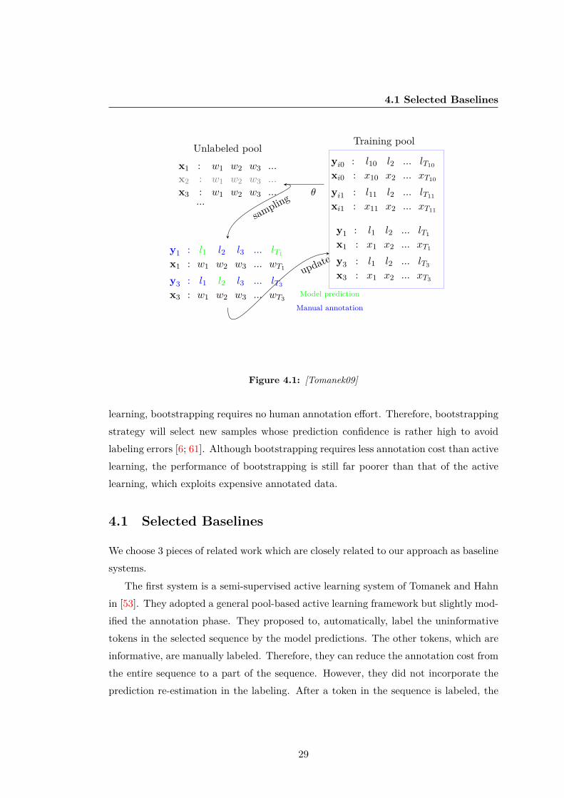
The first system is a semi-supervised active learning system of Tomanek and Hahnin [53]. They adopted a general pool-based active learning framework but slightly mod-ified the annotation phase. They proposed to, automatically, label the uninformativetokens in the selected sequence by the model predictions. The other tokens, which areinformative, are manually labeled. Therefore, they can reduce the annotation cost fromthe entire sequence to a part of the sequence. However, they did not incorporate theprediction re-estimation in the labeling. After a token in the sequence is labeled, the

29

4. RELATED WORK

.

.

..yi0 ..: ..l10 ..l2 ..... ..lT10

..xi0 ..: ..x10 ..x2 ..... ..xT10

..yi1 ..: ..l11 ..l2 ..... ..lT11

..xi1 ..: ..x11 ..x2 ..... ..xT11 .

..y1 ..: . ..l2 ..l3 ..... .

..x1 ..: ..w1 ..w2 ..w3 ..... ..wT1.

..y3 ..: ..l1 . ..l3 ..... ..lT3

..x3 ..: ..w1 ..w2 ..w3 ..... ..wT3

.Fully annotatedsource domain data

.Partially annotatedtarget domain data

Figure 4.2: [Tsuboi08]

..In .July .2003 ., .the .DPJ .and .the .Liberal .Party .led .by ....

.O .O .O .O .O .B-ORG .O .O .B-ORG .I-ORG .O .O ....

.ORG .ORG

..

Figure 4.3: [Neubig10]

model prediction of the other tokens may change. Figure 4.1 illustrates the frameworkdescribed in [53].

The second piece of work is a system of Tsuboi et al. which is trained on a partiallyannotated sequence [56]. They originally proposed a system for a domain adaptationtask. Given the fully-labeled-source-domain data, the unlabeled-target-domain data,and an external dictionary, they automatically annotated words in the target domaindata which are found in the dictionary, in order to obtain the partially annotated set.They finally trained a classifier using the fully-labeled-source and partially-labeled-target domain data as shown in Figure 4.2. While they automatically labeled theunlabeled sequences using an external dictionary, we propose a sampling method inactive learning framework to choose words for manual annotation.

The last system is another training approach for a partially annotated sequence.Neubig and Mori proposed a point-wise training method which ignores the dependencies

30

4.1 Selected Baselines

among output labels [34]. In other words, they defined factors or features on only theinput context. Figure 4.3 illustrates a feature without dependencies among outputlabels. Even though a sequence is partially labeled, we can simply train the classifierusing only the labeled parts.

31

4. RELATED WORK

32

Chapter 5

Proposed Framework

Although an active learning framework can reduce the annotation cost by choosing onlyinformative instances for labeling, there are still several rooms for further cost reductionin the sequence labeling problem. In this task, which is a structured output predictionproblem, the labeling is factorized to the subsequence or token labeling. Therefore, wecan also perform the active learning in the token level instead of the sequence level.

The informativeness of a token is defined by its prediction confidence. In this work,we employ the CRFs described in Chapter 2 for the training phase in the proposedframework. A CRFs classifier will predict an output label of a token with the followingmarginal probability:

P (yj = y′|x) = αj(y′|x) · βj(y′|x)Zθ,x,y

. (5.1)

We utilize this marginal probability as the prediction confidence for a token. When theconfidence is lower than a preset threshold, δ, the token may contain essential informa-tion which is not previously known to the model. Thus, we include this information tothe model by manually putting the correct label on this token. As in Figure 5.1, themarginal probability of the first two tokens are 0.40 and 0.80, which are lower than thethreshold, δ = .90. Therefore, an annotator should manually label both tokens.

After a token is labeled, the prediction confidence of all tokens in the sequence willincrease. In other words, the new information will propagate from the newly labeledtoken to the other neighboring tokens. If we re-estimate the confidence every time afterthe annotation of a token, we will substantially reduce the number of required labeledtokens.

33

5. PROPOSED FRAMEWORK

..DPJ.?

.B:0.40.I:0.30.O:0.30

.and.?

.O:0.80.I:0.20.B:0.00

.Liberal.?

.Party.?

.B:0.40

.O:0.30.I:0.30

.I:0.50.O:0.30.B:0.20

....

.......?

.x:

.y:

.DPJ

.B

.B:1.00.I:0.00.O:0.00

.and.?

.O:0.95.I:0.05.B:0.00

.Liberal.?

.Party.?

.B:0.95

.O:0.05.I:0.00

.I:0.99.O:0.01.B:0.00

....

.......?

.x:

.y:

.δ = 0.90

Figure 5.1: Marginal probability as the prediction confidence: The confidence thresholdis set to 0.90. There are 3 label types, B, I, and O. The figure after the label is the outputprobability of each label. After a token is labeled, the probability of all tokens will change.

Algorithm 2 Proposed active learning framework with the confidence re-estimationSs,t : {(x,yL)} is a set of all training sequences with current annotation at iterationt of subtask s

Ssel is a set of informative tokensx is an input tokenfor each s do

curmodel← train(Ss,1) {Initial training}repeat

Ssel ← Qtok(curmodel, Ss,t) {Sampling q tokens (at most): Section 5.3}for x ∈ Ssel do

Ss,t+1 ← update(Ss,t, x, label(x)) {Annotation: Section 5.1}end forcurmodel← train(Ss,t+1) {Training: Section 5.2}

until (|Ssel| < q) and (κ(Ss,t, Ss,t+1) > stop) {Stopping criterion: Section 5.5}Ss,final ← Ss,t+1

end forSfinal ← merge(Ss,final) {Merge training sets: Section 5.4}finalmodel← train(Sfinal)

34

5.1 Confidence Re-estimation in the Annotation

..x1 : w1 w2 w3 ... wT1

x3 : w1 w2 w3 ... wT3

...

(a) Given input sequence

.

.

..y1 ..: . ..l2 . ..... .

..x1 ..: ..w1 ..w2 ..w3 ..... ..wT1.

..y3 ..: . . ..l3 ..... .

..x3 ..: ..w1 ..w2 ..w3 ..... ..wT3

. .....

(b) 1st annotation

.

.

..y1 ..: . ..l2 ..l3 ..... .

..x1 ..: ..w1 ..w2 ..w3 ..... ..wT1.

..y3 ..: ..l1 . ..l3 ..... .

..x3 ..: ..w1 ..w2 ..w3 ..... ..wT3

. .....

(c) 2nd annotation

.

.

..y1 ..: . ..l2 ..l3 ..... .

..x1 ..: ..w1 ..w2 ..w3 ..... ..wT1.

..y3 ..: ..l1 . ..l3 ..... ..lT3

..x3 ..: ..w1 ..w2 ..w3 ..... ..wT3

. .....

(d) 3rd annotation

.

.

..y1 ..: ..l1 ..l2 ..l3 ..... ..lT1

..x1 ..: ..w1 ..w2 ..w3 ..... ..wT1.

..y3 ..: ..l1 ..l2 ..l3 ..... ..lT3

..x3 ..: ..w1 ..w2 ..w3 ..... ..wT3

. .....

(e) Final annotation

Figure 5.2: Confidence re-estimation in the annotation. An annotator labels on token inthe sequence in each step ((b) to (e)). At the final iteration, low-informative tokens (inbold figures) are labeled by the model prediction.

We adopt the general active learning framework in Chapter 3 and integrate theconfidence re-estimation in the annotation (Section 5.1), the training (Section 5.2), andthe sampling phases (Section 5.3). The outline of the proposed framework is shownin Algorithm 2. We also propose the simplified sampling to reduce the computationaltraining time (Section 5.4) and discuss the stopping criterion in Section 5.5.

5.1 Confidence Re-estimation in the Annotation

We assume that the human annotation is always correct. When a token is manuallyannotated, the classifier will select the human annotation as the output label. Hence,the prediction probability of the labeled token is always 1.0. We propose to re-estimatethe confidence after every single token annotation. An example of a sequence annotationis shown in Figure 5.2.

Given the input sequence in Figure 5.2a, the most informative token in the sequenceis selected and labeled by the annotator as shown in Figure 5.2b. Subsequently, the

35

5. PROPOSED FRAMEWORK

prediction confidence of all tokens in the sequences is re-estimated. Then, the nexthighest informative token is selected and labeled until there is no informative tokenleft in the sequence. Finally, all of the uninformative tokens are labeled by the modelprediction. Therefore, we can obtain a labeled sequence for training. However, theannotator only puts labels to some tokens in the sequence. Figure 5.2e shows thelabeled sequence for the training. Labels in boldface are automatically annotated,while the other tokens are manually annotated.

5.2 Confidence Re-estimation in the Training

The conventional CRFs described in Section 2.2 require a sequence to be fully an-notated. We can annotate sequences using both the human annotation and machineannotation as done in Section 5.1. However, the accuracy of the models in early itera-tions is usually low, which makes the prediction confidence from those early models notreliable. In addition, adding these incorrectly predicted outputs to the training set willprevent the model from achieving high accuracy. These errors remain in the trainingdata and are not recovered, even though the classifier becomes more accurate in lateriterations.

We propose to re-estimate the output prediction in every iteration, instead of fixinglabels to the prediction of the model in early iterations. When the classifier becomesmore accurate in later iterations, the prediction will also be more accurate. We directlyestimate the prediction in the training phase using CRFs for partially annotated se-quence proposed by Tsuboi et al. in [56]. They proposed to fill the unlabeled tokenswith their marginalized output. In other words, we implicitly annotate the unlabeledtokens with all possible output labels, augmented with their prediction probabilities.As a result, when the model becomes more precise, these implicitly annotated tokenswill also be more precise.

Figure 5.3 shows an example of the re-estimation in the training. We sample andannotate tokens similar to the process done in Section 5.1. The difference is in the finalannotation. We do not put the predicted labels on high-confidence tokens. Instead, weuse the implicit annotation through the re-estimation in the training phase.

36

5.3 Token Sampling Strategy

.

.

..x1 ..: ..w1 ..w2 ..w3 .....

..x2 ..: ..w1 ..w2 ..w3 .....

..x3 ..: ..w1 ..w2 ..w3 .....

. .....

.Unlabeled pool

.

..y10 ..: ..l10 ..l2 ..... ..lT10

..x10 ..: ..x10 ..x2 ..... ..xT10

..y11 ..: ..l11 ..l2 ..... ..lT11

..x11 ..: ..x11 ..x2 ..... ..xT11

.Training pool

.

..y1 ..: . ..l2 ..l3 ..... .

..x1 ..: ..w1 ..w2 ..w3 ..... ..wT1.

..y3 ..: ..l1 . ..l3 ..... .

..x3 ..: ..w1 ..w2 ..w3 ..... ..wT3

.Manual annotation

.

..y1 ..: . ..l2 ..... .

..x1 ..: ..x1 ..x2 ..... ..xT1

..y3 ..: ..l1 . ..... .

..x3 ..: ..x1 ..x2 ..... ..xT3

.θ

.sampling

.update

Figure 5.3: Confidence re-estimation in the training. An annotator labels one token in thesequence in each step ((b) to (e)). No token is explicitly labeled by the model prediction.

5.3 Token Sampling Strategy

We have discussed that the accuracy of the classifier has an effect to the reliabilityof the prediction confidence. We can lessen the impact of a poor classifier from earlyiterations by re-estimating the prediction in the training process. In this section, weargue that the model accuracy also affects the sampling process, since the samplingalso depends on the prediction confidence. Desired sampling should be able to retrievemany informative tokens. Therefore, we can expect less efficient sampling results fromearly models than from those in later iterations.

When many tokens in a sequence are annotated, the probability of the other un-labeled tokens is generally high. If the labeled tokens are uninformative or less-informative tokens, we will miss the chance to annotate other informative tokens.Therefore, we need to re-train the model every time after a single token in a sequenceis annotated. However, the training cost will be extremely high. We, instead, proposeto sample a set of sequences and annotate only the highest informative token in eachsampled sequence. Specifically, we sort all tokens in the corpus by their confidence

37

5. PROPOSED FRAMEWORK

scores in ascending order. In other words, we perform token sampling instead of se-quence sampling, in order to utilize the probability re-estimation in the sampling. Asequence may be sampled several times if there are several informative tokens in thesequence.

5.4 Simplified Sampling

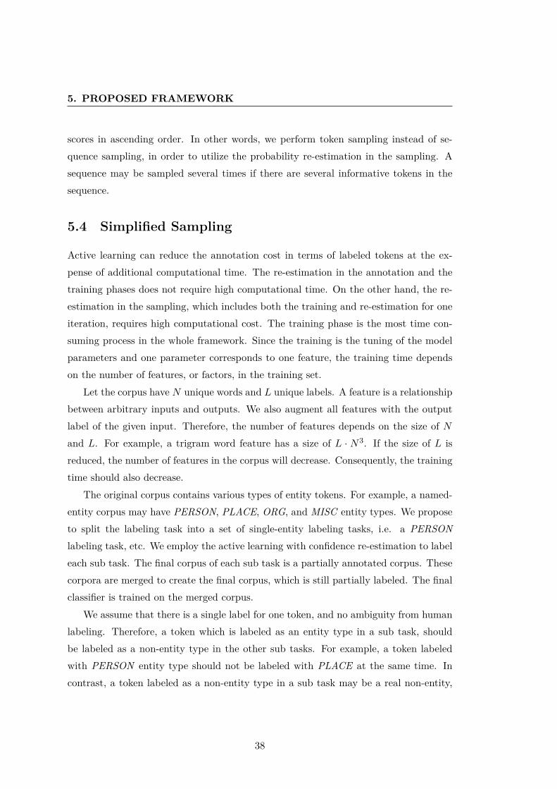
Active learning can reduce the annotation cost in terms of labeled tokens at the ex-pense of additional computational time. The re-estimation in the annotation and thetraining phases does not require high computational time. On the other hand, the re-estimation in the sampling, which includes both the training and re-estimation for oneiteration, requires high computational cost. The training phase is the most time con-suming process in the whole framework. Since the training is the tuning of the modelparameters and one parameter corresponds to one feature, the training time dependson the number of features, or factors, in the training set.

Let the corpus have N unique words and L unique labels. A feature is a relationshipbetween arbitrary inputs and outputs. We also augment all features with the outputlabel of the given input. Therefore, the number of features depends on the size of Nand L. For example, a trigram word feature has a size of L · N3. If the size of L isreduced, the number of features in the corpus will decrease. Consequently, the trainingtime should also decrease.

The original corpus contains various types of entity tokens. For example, a named-entity corpus may have PERSON, PLACE, ORG, and MISC entity types. We proposeto split the labeling task into a set of single-entity labeling tasks, i.e. a PERSONlabeling task, etc. We employ the active learning with confidence re-estimation to labeleach sub task. The final corpus of each sub task is a partially annotated corpus. Thesecorpora are merged to create the final corpus, which is still partially labeled. The finalclassifier is trained on the merged corpus.

We assume that there is a single label for one token, and no ambiguity from humanlabeling. Therefore, a token which is labeled as an entity type in a sub task, shouldbe labeled as a non-entity type in the other sub tasks. For example, a token labeledwith PERSON entity type should not be labeled with PLACE at the same time. Incontrast, a token labeled as a non-entity type in a sub task may be a real non-entity,

38

5.5 Stopping Criterion

Iterations1 2 3 4

.

.

.. ..N .. ..

.. .. .. ..N

.. ..B .. ..

.. ..N .. ..

.

.

..B ..N .. ..

.. .. .. ..N

.. ..B ..N ..

.. ..N .. ..B

.

.

.. ..R .. ..

.. .. .. ..R

.. ..N .. ..

.. ..N .. ..

.

.

.. ..R ..N ..

.. .. .. ..R

..N ..N .. ..

..R ..N .. ..

5 6 Final Corpus

.

.

.. .. .. ..G

.. ..G .. ..

.. ..N .. ..

.. ..N .. ..

.

.

..N .. .. ..G

.. ..G .. ..N

.. ..N .. ..N

.. ..N ..G ..

.

.

..B ..R .. ..G

.. ..G .. ..R

.. ..B .. ..

..R ..N ..G ..B

Figure 5.4: An example of simplified sampling

or an entity of the other types. A token is regarded as a non-entity token if and only ifit is labeled as a non-entity type in all sub tasks. Otherwise, the token is left unlabeledin the merged corpus.

However, we found that few non-entity tokens are labeled in all sub tasks. Therefore,the merged corpus will contain mostly entity tokens, lacking non-entity tokens. Thismerged corpus is inappropriate for the training. We propose to add non-entity labels tothe training set by using the model prediction of all sub tasks. There may be conflictsamong the model predictions. In such cases, we leave the tokens unlabeled.

An example of the simplified sampling is shown in Figure 5.4. Let us have 4 classlabels, the B, the R, the G entity classes, and the N non-entity class. Instead of askingan annotator to determine the class label of a token among 4 label candidates, we dividethe tasks into 3 subtasks, the B labeling, the R labeling, and the G labeling. After allsub tasks are done, we merge the partially annotated data of each sub task togetherand train the final model using the merged data.

5.5 Stopping Criterion

The stopping criterion is also a prominent key of active learning to reduce the anno-tation cost by stopping the labeling when the accuracy converges to the desired level.

39

5. PROPOSED FRAMEWORK

Firstly, we predict the output of all training sequences using the current model ineach iteration. Note that the output of a labeled token is perfect, and always correct.Secondly, we measure the similarity between the prediction of the models from twoconsecutive iterations using Kappa statistic [11], which is a measure of inter-annotatoragreement. The probability of two corpus annotation, Ao is

Ao =nAgree

nAll, (5.2)

where nAgree and nAll are the number of prediction agreement, and the number ofall predictions, respectively. Let the number of label l predictions in a corpus i be ni

l.The probability that the agreement occurs by chance is

Ae =∑l

n1l n

2l

(∑

l n11)

2. (5.3)

We can calculate the Kappa statistic, κ, by the following equation:

κ =Ao −Ae

1−Ae. (5.4)

When κ is high, it indicates that the agreement does not occur by chance, and the twocorpora are very similar. The learning can be stopped when κ between iterations arehigh enough. We empirically tuned κ and set the threshold to 0.9999. When κ exceedsthe threshold, the labeling will be stopped.

40

Chapter 6

Experiments

6.1 Data and Evaluation

We evaluate the proposed framework on two tasks, the English all-phrase chunking andthe English named-entity recognition tasks.

6.1.1 CoNLL2000

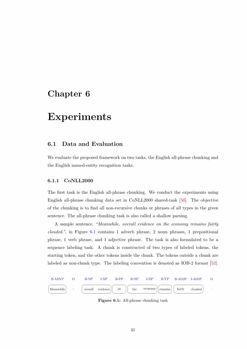
The first task is the English all-phrase chunking. We conduct the experiments usingEnglish all-phrase chunking data set in CoNLL2000 shared-task [50]. The objectiveof the chunking is to find all non-recursive chunks or phrases of all types in the givensentence. The all-phrase chunking task is also called a shallow parsing.

A sample sentence, “Meanwhile, overall evidence on the economy remains fairlyclouded.”, in Figure 6.1 contains 1 adverb phrase, 2 noun phrases, 1 prepositionalphrase, 1 verb phrase, and 1 adjective phrase. The task is also formulated to be asequence labeling task. A chunk is constructed of two types of labeled tokens, thestarting token, and the other tokens inside the chunk. The tokens outside a chunk arelabeled as non-chunk type. The labeling convention is denoted as IOB-2 format [52].

..B-ADVP .O .B-NP .I-NP .B-PP .B-NP .I-NP .B-VP .B-ADJP .I-ADJP .O

.Meanwhile ., .overall .evidence .on .the .economy .remains .fairly .clouded ..

Figure 6.1: All-phrase chunking task

41

6. EXPERIMENTS

Table 6.1: CoNLL2000 data; Number of sequences, tokens, chunk types and chunks ofall-phrase. NP chunking is the simplified task on the same data set.

Dataset Num. Seq. Num. Tok. Num.Chunk types Num. ChunksAll-phrase Chunking

training 8936 211727 22 106978test 2012 47377 19 23852NP-Chunking

training 8936 211727 3 55081test 2012 47377 3 12422

Therefore, the output is a label sequence of the same length of the corresponding inputsequence.

The data statistics of CoNLL2000 is shown in Table 6.1. We also simplify thedata set to one-phrase, NP, chunking task in order to compare the performance of theproposed system between the single-entity and all-entity tasks.

We extract the features following [49] and employ a CRFs classifier to predict theoutput of each token. We set the context window to extract features and let the currentword be the center of the window. All features are binary features. The list of featuresis as follows:

• Word n-gram: unigrams in the word window of size 5, bigrams in the window ofsize 3

• Part-of-speech n-gram: unigrams, bigrams and trigrams in the window of size 5

• Transition: label of the previous word

Note that the transition function makes the task a structured output problem. Withoutthis feature, the token labeling becomes a simple classification task.

6.1.2 CoNLL2003

A named entity is a phrase that contains a name of person, organization, place, time,and quantity [51]. The named entity recognition task is the task to find all namedentities in a given sentence. We perform the experiment using English data set fromCoNLL2003 shared-task [51]. A named entity chunk is also constructed of two types of

42

6.1 Data and Evaluation

Table 6.2: CoNLL2003 data: Number of sequences, tokens, chunk types and chunks ofEnglish NER task.

Dataset Num. Seq. Num. Tok. Num. Chunk types Num. ChunksEnglish NERtraining 14987 204567 8 23499test 3684 46666 8 5648

Table 6.3: Word types and examples

Description Examplesstarts with capital letter Confidence, September, Butall capital letters PLC, GNP, Acontains both uppercase and lowercase letters anti-American, Chancellor, Lawsonsingle digit 1, 2, 3contains only digits 16, 1988, 190contains at least two periods U.K., A.P., F.S.Bends with a period Ala., p.m., vs.contains a dash year-ago, 1-800-453-9000, 10-foldsingle character A, a, bcontains punctuation US$, #, /,/contains quotation ’s, I’m, n’t

tokens. The data set uses slightly different representation of labels from the chunkingdata set. Instead of using the starting and in-chunk labels, all tokens are labeled asin-chunk tokens. Only if there are two consecutive entities, the starting token of thesuccessor is labeled as the starting label. The representation is IOB-1 format [39].

Again, we extract features and predict the chunk label using a CRFs classifier. Weset the context window to extract features and let the current word be the center of thewindow. All features are binary features. The list of features in this task is summarizedas follows:

• Word n-gram: unigrams in the word window of size 5

• Previous and following word sequence: a 4-word sequence before and after thecurrent word

43

6. EXPERIMENTS

Table 6.4: Prediction confusion marix

is a chunk in the corpus is not a chunk in the corpusis a predicted chunk tp fp

is not a predicted chunk fn tn

• Lowercase n-gram: unigrams and bigrams of lowercase words in the window ofsize 5, a trigram word in the window of size 3

• Word type: types summarized in Table 6.3

• Part-of-speech n-gram: unigrams, bigrams, and trigram in the window of size 5.Part-of-speech information is provided in the data set.

• Chunk type n-gram: unigrams, bigrams, and trigram in the window of size 5.Chunk type, e.g. NP, is also provided in the data set.

• Character prefix and suffix: 2- and 3-character prefixes and suffixes of the inputword. For example, Ame is 3-character prefix of the word American.

• Transition: label of the previous word

6.1.3 Evalutaion

The objective of the proposed framework is to achieve the supervised accuracy withas little annotation effort as possible. The supervised accuracy is the accuracy of asystem trained on a fully annotated corpus. We measure the performance of eachtrained system by CoNLL chunk F1 [50]. We use the word accuracy interchangeablywith F1 in this thesis.

A chunk is counted as correct if and only if the output of all tokens in the chunkare correctly predicted (tp). All other predicted chunks are counted as false predictedchunks (fp). Finally, the incorrectly predicted chunks are counted to be unrecognizedchunks (fn). The rest are any tokens stay outside of a chunk (tn). We summarizethese counts in the confusion matrix, in Table 6.4.

The precision (Pr) and recall (Re) are calculated by the following equations:

Pr =tp

tp+ fp, (6.1)

44

6.2 Parameter Tuning

Re =tp

tp+ fn. (6.2)

The CoNLL chunk F1 is the harmonic mean of the precision and recall:

F1 =2(Pr)(Re)

Pr +Re. (6.3)

We also evaluate the statistical difference of F1 between systems using McNemar test[21]. The null hypothesis of the test states that the prediction errors of two classifiersare independent of each other. Let the errors from a classifier i be erri. The McNemartest is given by

χ2 =(|err1 − err2| − 0.5)2

err1 + err2. (6.4)

We will reject the hypothesis, i.e. the difference is statistically significant, when χ2 ishigher than 3.84 with α = 0.05.

We divide the annotation effort into 2 types. The first type is the number oftokens, or words, that a human annotator put a label for. We use the percentage of theannotated tokens in the whole corpus to represent this annotation cost. The other typeis the computational time required in the full annotation task. Since active learning isan iterative method, a human is asked to annotate new tokens in every iteration. Weassume that the annotation cost of each token is equal. We measure the idle time ofthe annotator in each iteration, also the cumulative idle time of the annotator1. Notethat we did not consider the actual annotation time of a human annotator.

6.2 Parameter Tuning

6.2.1 Initial Training Set

We compared the F1 of the proposed framework starting from the collection of shortsequences, long sequences and random sequences in Figure 6.2. Each initial set consistsof 50 fully annotated sequences. The confidence threshold is set to 0.99. New 500most informative tokens are selected and manually labeled in each iteration of activelearning. In Figure 6.2, long-sequence initial set leads to the supervised accuracy withfewer labeled tokens than when starting with the other initial sets.

1We conducted all experiments on 3.00GHz Xeon E5450 server using 4 cpus. Our CRFs classifierwas implemented in C.

45

6. EXPERIMENTS

87

88

89

90

91

92

93

94

95

2 3 4 5 6 7

0 50 100 150 200 250 300

F1

%Manually annotated tokens

CoNLL2000 NP Chunking Proposed δ t=0.99

Time (min)

SupRandom start

Short startLong start

Figure 6.2: F1 on the systems trained of different initial sets. Lines represent the numberof labeled tokens. Points of the same color represent the CPU time.

Note that long sequences contain more tokens than short sequences. Although weassume that the annotation cost of all tokens is equal, an annotator should spend moreannotation effort on the long-sequence initial set. However, the initial set contains only50 sequences, which may not expect much annotation effort. Moreover, points on thetop of Figure 6.2 show that the long-sequence initial set also achieves higher accuracywith similar CPU time. Hence, we will use 50 longest sequences as our initial set in allof the following experiments.

6.2.2 Sampling Size

Sampling size is the number of instances given to an annotator for labeling in oneiteration. Sampling size is also another decisive factor in active learning. When thesampling size is large, some less informative instances are sampled for annotation. Onthe other hand, one extreme setting is to annotate one instance per iteration, butthe CPU time will tremendously increase. We should consider these two costs, whichbecome a trade-off of each other.

We perform the analysis using the proposed framework without the simplified sam-pling on NP chunking data set. The sampling size is set to 50, 500, and 1000 tokens

46

6.2 Parameter Tuning

87

88

89

90

91

92

93

94

95

2 3 4 5 6 7

0 100 200 300 400 500 600 700

F1

%Manually annotated tokens

CoNLL2000 NP Chunking Proposed δ=0.99

Time (min)

Supqsize=50

qsize=500qsize=1000

Figure 6.3: F1 of the systems with different sampling sizes. Lines represent the numberof labeled tokens. Points of the same color represent the CPU time.

per iteration. The lines in Figure 6.3 show that there is no significant difference in theF1 achievement of individual sampling size settings. From the points of small samplingsize setting, the setting significantly increases the idle time cost. We try to limit theidle time per iteration to several minutes. In the real annotation scenario, the idle timebecomes a short break for a human, before starting labeling the next iteration. Fromthe experiments, we found that the sampling size of 500 tokens is the most efficient.

6.2.3 Confidence Threshold

The last parameter is the prediction confidence threshold, δ, which defines the informa-tiveness of a token. There is a trade-off between the high and the low-threshold settings.The reliability of the model prediction is high when the prediction confidence is high.Labeling all tokens in the selected sequence is equivalent to the threshold at positiveinfinity. On the other hand, the threshold at zero is equivalent to the self-trainingbootstrapping system. High-threshold setting will require a high number of labeledtokens. Although we can reduce the number of labeled tokens using a low threshold,we expect more risk of increasing incorrectly predicted labels to the training set, whichleads to low-accuracy performance.

47

6. EXPERIMENTS

87

88

89

90

91

92

93

94

95

2 3 4 5 6 7

0 50 100 150 200 250 300

F1

%Manually annotated tokens

CoNLL2000 NP Chunking Proposed

Time (min)

Supδ=0.60δ=0.90δ=0.99

Figure 6.4: F1 of the systems with different confidence threshold. Lines represent thenumber of labeled tokens. Points of the same color represent the CPU time.

We conduct the experiment using the re-estimation in the annotation, the training,and the sampling. Our data set is the NP chunking set. Lines in Figure 6.4 show,as expected, that the low-confidence threshold setting leads to fast convergence, andachieves low F1. The difference of F1 at the convergence of the system with the thresholdat 0.90 and 0.99 is not statistically significant. The result also confirms that high-threshold setting may also lead to over-annotation, similar to the large sampling sizecase.

6.3 Baseline Systems

There are several pieces of work related to the proposed system. In this section, wewill compare this related work before comparing them to the proposed system in thefollowing sections.

[Sup]: The F1 of this straightforward supervised system trained on a fully anno-tated corpus is the upper-bound of all systems. Our goal is to achieve this supervisedF1 with the smallest number of labeled tokens.

[Pointwise]: Neubig and Mori proposed a point-wise training framework in the

48

6.3 Baseline Systems

Table 6.5: Comparison between baseline systems on NP chunking task. Boldface figuresare F1 which are not statistically different from the supervised F1.

Systems F1 %Labeled tokens Training time (sec)[Sup] 93.86 100.00 521[Pointwise] 92.52 100.00 57[Bootstrap] 89.05 1.43 1302[AL] 93.85 100.00 4019[Tomanek09] δ = 0.99 92.91 5.48 3432

domain adaptation task, which ignores the dependencies among the output labels [34].We emulate their system in a supervised manner. Specifically, we use all features exceptthe transition feature. The supervised point-wise system will provide the upper boundaccuracy of a point-wise active learning system.

The first half of Table 6.5 are the non-iterative systems. Both systems are trainedon the same fully annotated corpus. However, [Pointwise] achieved significantly lowerF1 than [Sup]. Hence, we conclude that the transition features in [Sup] are responsiblefor the large gap between the two F1 achievement. All of the following settings willinclude the transition features.

The other baselines are iterative sequence-sampling systems. All systems start withthe same long-sequence initial set. The query size is set to 500 sequences per iteration.The confidence threshold, δ, is set to 0.99.

[Bootstrap]: The first iterative baseline is a bootstrapping system, whose high-confidence tokens are annotated with the model prediction. Labels of low-confidencetokens are implicitly estimated in the training.

[AL]: The second iterative baseline is a fully supervised active learning system,whose training tokens are manually labeled. [AL] becomes almost exactly the same as[Sup] after we label the whole training set. The only difference between [AL] and [Sup]is the sentence ordering in the training set.

[Tomanek09]: The last baseline is the system proposed by Tomanek and Hahn[53]. In each sampled sentence, the low-confidence tokens are manually labeled, whilethe high-confidence tokens are automatically labeled by the model prediction.

Figure 6.5 shows the correlation between the number of labeled tokens and F1 of eachbaseline. Note that the F1 of [Sup] does not vary since we train the tagger once with

49

6. EXPERIMENTS

86

88

90

92

94

2 3 4 5 6 7

F1

%Manually annotated tokens

CoNLL2000 NP Chunking

SupPointwiseBootstrap

ALTomanek09 δ=0.99

Figure 6.5: F1 comparison among baseline systems

87

88

89

90

91

92

93

94

95

0 10 20 30 40 50 60 70 80

F1

Time (min)

CoNLL2000 NP Chunking

SupPointwiseBootstrap

ALTomanek09 δ=0.99

Figure 6.6: Training time comparison among baseline systems

50

6.4 Confidence Re-estimation in the Annotation

the whole training set. We just draw a straight F1 line of [Sup] for reference. Similarly,the number of manually labeled tokens of [Bootstrap] is also fixed to the number oftokens in the initial set. However, the F1 of [Bootstrap] varies since we gradually addtokens to the training set. We draw a straight line of final F1 of [Bootstrap] vs. numberof labeled tokens.

The straight line at the bottom of the figure is the F1 of the bootstrapping system([Bootstrap]), which indicates that we can hardly learn new information from unlabeledtokens. Although the F1 of [Bootstrap] slightly increases, its best F1 is still far worsethan any other baselines that include more labeled tokens.

There are two learning curves in the middle of Figure 6.5. The bottom curve is [AL],which has a low-learning rate. We cut the learning curve to first 15k labeled tokensdue to the limited space. However, the F1 of [AL] gradually increased and reached thesupervised level when nearly 150k of tokens are labeled. The other curve represents thelearning rate of [Tomanek09]. Although [Tomanek09] achieved much higher F1 than[Bootstrap] with 4% additional labeled tokens, its best F1 is still far worse than thesupervised F1.

Figure 6.6 shows the training time of each baseline. The training time of few labeledtokens is rather fast. We will discuss the training time later in Section 6.7.

Finally, we compare the performance of iterative baselines to non-iterative baselinesin Table 6.5. In terms of the number of manually labeled tokens, active samplingmethods obviously require fewer labeled tokens and achieve higher F1 than non-iterativemethods. Since the model becomes more precise in later iterations, we need to label fewtokens but still achieve high F1. In contrast, the iterative methods have a disadvantagein the training time since we have to re-estimate the model parameters in each iteration.In this thesis, we give priority to the labeled token cost.

6.4 Confidence Re-estimation in the Annotation

In the annotation phase, the re-estimation can reduce the annotation cost on tokens inthe following categories. The first type is the tokens which are correctly predicted bythe model, but have low-prediction confidence. After the re-estimation, these tokenswill gain more prediction confidence. When the confidence passes the threshold, we canreduce the annotation cost on these tokens but still have the correct prediction. The

51

6. EXPERIMENTS

0

2000

4000

6000

8000

10000

12000

14000

0 2 4 6 8 10 12 14 16 18

Num

ber

of to

kens

Iteration

CoNLL2000 NP Chunking

correct-unchangetoCorrect

toIncorrectincorrect

Figure 6.7: Label changes after re-estimation in the annotation phase

second type is the tokens with the outputs which are previously incorrectly predicted,

but their outputs are corrected after the re-estimation.

From Figure 6.7, labels of the most tokens remain unchanged after the re-estimation.

However, the prediction confidence of each token is increased. Therefore, we are re-

quired to label fewer tokens but still achieved the system with similar accuracy to the

system without the re-estimation. The result is also shown in Figure 6.8 that the F1

scores before and after re-estimation were not significantly different.

We also compute the kappa statistics between the corpora before and after the

re-estimation. The agreement between the two corpora has κ = 0.99. This kappa

value indicates that both annotated corpora are highly similar. We conclude that the

re-estimation does not significantly alter the predicted output but raises the confidence

of some tokens to exceed the threshold level. Therefore, we can reduce the annotation

on these tokens. However, we cannot improve the F1 of the system since the corpora

before and after re-estimation are remarkably similar.

52

6.5 Confidence Re-estimation in the Training

87

88

89

90

91

92

93

94

95

2 3 4 5 6 7

F1

%Manually annotated tokens

CoNLL2000 NP Chunking δ=0.99

SupTomanek09

ReEst(Annotation)

Figure 6.8: F1 of the model with re-estimation in the annotation phase

0

1

2

3

4

5

6

7

0 10 20 30 40 50 60 70 80 90 100

%E

rror

s in

trai

ning

dat

a

%Manually annotated tokens

CoNLL2000 NP Chunking δ=0.99

ALTomanek09

ReEst(Train)

Figure 6.9: Errors in the training set with and without re-estimation

53

6. EXPERIMENTS

6.5 Confidence Re-estimation in the Training

We conduct an experiment using a fully annotated corpus as a gold standard, andevaluate the prediction accuracy of the model in each iteration on the entire trainingcorpus against the gold standard. The accuracy of a labeled token will be 1.0. Theaccuracy of the other tokens depends on the prediction confidence. If an incorrectlypredicted label is added into the training set, the accuracy of that token becomes zero.On the other hand, if we estimate the label in training, the error will depend on theprediction confidence. The result in Figure 6.9 shows that every setting starts withthe same error level of the same initial set. When more tokens are labeled, the errorsdecrease because of the labeled tokens themselves and the improved accuracy of themodel. Errors of [AL] continue decreasing to zero when all tokens are annotated. Incontrast, errors of [Tomanek09] sharply decrease but stop early while errors are stillhigh. Therefore, the model trained on this erroneous training corpus achieved lower F1

than the fully supervised model.The proposed framework, which implicitly estimates the output labels in the train-

ing, does not suffer much from the incorrect prediction. Although the errors are high inearly iterations similar to [Tomanek09], the prediction is automatically corrected aftera model becomes more accurate in later iterations. In contrast, the prediction errorsof [Tomanek09] remain in the corpus and cannot be corrected. As a result, the errorcurve of [ReEst(Train)] sharply decreases, which is similar to the curve of [Tomanek09]but continues decreasing to lower error level.

Figure 6.10 shows the F1 among the system without any re-estimation ([Tomanek09]),the system with the re-estimation in the training ([ReEst(Train)]), and the system withthe re-estimation in both the training and the annotation phases ([ReEst(Annotation,Train)]).Although the F1 of [ReEst(Train)] reached a higher level than [Tomanek09], it requiresmore labeled tokens. However, after we combine the re-estimation in the annotationphase, we can reduce the annotation cost but keep the high F1 level as stated in Section6.4.

6.6 Token Sampling

We compare between the 2 sampling strategies, the sequence sampling and the tokensampling. In the token sampling, 500 sequences with the most informative tokens are

54

6.7 The Computational Time

87

88

89

90

91

92

93

94

95

2 3 4 5 6 7 8

F1

%Manually annotated tokens

CoNLL2000 NP Chunking δ=0.99

SupAL

Tomanek09ReEst(Train)

ReEst(Annotation,Train)

Figure 6.10: F1 of the model with and without the re-estimation in the training phase

sampled. Only the most informative tokens in each selected sequence will be annotatedin one iteration. In the sequence sampling, 500 most informative sequences are sampled.All informative tokens in the selected sequences are annotated. The [Seq-Sampling]system is exactly the same system as the [ReEst(Annotation,Train)] in Section 6.5. Inboth of the sampling strategies, high-confidence tokens, which are uninformative, areleft for the implicit annotation in the training phase.

Figure 6.11 shows that the token sampling strategy, which provides more opportu-nity for confidence re-estimation than the sequence sampling, achieves higher F1, withmore labeled token cost. We also compare the token sampling with different confidencethreshold. The system with δ = 0.90 also achieves the supervised F1 with fewer labeledtokens than the system with higher threshold, δ = 0.99.

6.7 The Computational Time

The re-estimation in each process can reduce the annotation cost in terms of labeledtokens, but the re-estimation requires additional computational cost. There are severalfactors that affect the computational cost. In this thesis, we take 3 factors into account,the corpus size, the re-estimation step, and the number of label candidates. We will

55

6. EXPERIMENTS

87

88

89

90

91

92

93

94

95

2 3 4 5 6 7 8

F1

%Manually annotated tokens

CoNLL2000 NP Chunking

SupAL

Seq-sampling δ=0.99Tok-Sampling δ=0.90Tok-Sampling δ=0.99

Figure 6.11: F1 of the sequence sampling and the token sampling

discuss the first two factors in this section. The last factor will be discussed in Section6.8.

We plot the number of tokens/sequences and the CPU time of [AL] using green lineand point in Figure 6.12. A larger corpus which contains more sequences, will needmore training time than a smaller corpus; since the training will evaluate the currentparameters on all training sequences.

Secondly, we compare the computational time of [AL] and [ReEst(Annotation)] todetermine the effect of the re-estimation in the annotation. Although the second settingrequires additional time in the re-estimation, the overall CPU time is less than the timein [AL]. We argue that the re-estimation in the annotation takes few seconds, but thetraining time is substantially reduced due to the automatically labeled tokens. Thereare few differences between the model prediction and the automatically annotated labelof the high-confidence tokens. Therefore, the optimization will not take a long time forthe updating parameters of these tokens.

Thirdly, we study the impact of the re-estimation in the training phase. FromFigure 6.12, [ReEst(Train)] requires less training time than [AL]. We suggest againthat the optimization takes a short time since there are few differences between thepredicted and the marginalized labels. Finally, [ReEst(Annotation,Train)] requires less

56

6.8 The Simplified Sampling

0

10

20

30

40

50

60

70

0 50000 100000 150000 200000

Tim

e (m

in)

Number of tokens

CoNLL2000 NP Chunking δ=0.99

ALReEst(Annotation)

ReEst(Train)ReEst(Annotation,Train)

Figure 6.12: CPU time of the training on different corpus size

time than [ReEst(Train)] because the re-estimation in the annotation makes the pre-diction confidence of tokens relatively stable and will not change in later iterations.

6.8 The Simplified Sampling

In this section, we estimate the impact of the number-of-label-candidate factor at thetraining time, and the simplified sampling strategy which is intended to reduce thetraining cost due to this factor.

We split the all-phrase labeling task into several single-type labeling tasks. Wecompare the CPU time of a single iteration of [AL] between the two labeling strategiesusing CoNLL2000 data set in Figure 6.13. The original and simplified data sets haveidentical training instances. The difference is only the number of target classes, whichwill affect the feature complexity. The simplified chunking tasks clearly require lesscomputational time.

In the last experiment, we compare the cumulative CPU time of the simplifiedlabeling, and all phrase labeling in Figure 6.14. Although the all-phrase chunking issplit to several sub tasks, the cumulative CPU time of the simplified labeling is stillcomparable to the full labeling.

57

6. EXPERIMENTS

AL

Tok-Sampling-0.90

Tok-Sampling-0.99

Simplified-0.90

Simplified-0.99

0 100 200 300 400 500 600 700 800 900 1000 1100

Time (sec)

CoNLL2000: Training time in one iteration

Figure 6.13: Single-iteration CPU time of the all-phrase chunking and single-type chunk-ing tasks

500

0

600

0

700

0

800

0

900

0

100

00

3200

0

3300

0

3400

0

3500

0

Time (sec)

CoNLL2000: Cumulative Training time

8066

AL

3271

2T

ok-S

ampl

ing-

0.90

7363

Sim

plifi

ed-0

.90

3322

1T

ok-S

ampl

ing-

0.99

9559

Sim

plifi

ed-0

.99

Figure 6.14: Cumulative CPU time of the all-phrase chunking and single-type chunkingtasks

58

6.9 Final Result

Table 6.6: Result of each system on CoNLL2000 and CoNLL2003. Boldface figuresindicate that the F1 is not significantly different from the supervised F1. Shaded cellsshow the main disadvantage of the systems.

CoNLL2000Systems F1 Num. Lab. Tokens Time/Iter Cum. Time[AL] 93.42 95.54 480 8066[Tok-Sampling]-0.90 93.41 5.87 723 32712[Tok-Sampling]-0.99 93.46 7.09 772 33221[Simplified]-0.90 92.98 7.67 83 7363[Simplified]-0.99 93.14 11.68 88 9559

CoNLL2003Systems F1 %Labeled Tokens Time/Iter Cum.Time[AL] 81.49 88.52 1972 42056[Tok-Sampling]-0.90 81.21 7.23 2790 78118[Tok-Sampling]-0.99 81.33 9.29 1707 59762[Simplified]-0.90 80.46 6.35 560 47244[Simplified]-0.99 81.11 7.21 638 58817

6.9 Final Result

Table 6.6 shows the comparison of the proposed framework to the [AL] baseline. Theproposed all-type labeling system achieves the supervised F1 on both data sets at theexpense of longer average idle time of an annotator between iterations. On the otherhand, the proposed single-type labeling system achieves slightly lower F1 with muchshorter idle time than the baseline system. The cumulative CPU time of the simplifiedtask is also close to the cumulative CPU time of the [AL] baseline.

59

6. EXPERIMENTS

60

Chapter 7

Conclusion and Future Work

We have proposed an active learning framework for sequence labeling that incorporatesthe prediction confidence in the annotation, re-training, and sampling phases of activelearning. The proposed framework could succeed in reducing the manually labeledtokens from the supervised learning, but still be able to achieve the supervised F1.The confidence re-estimation could increase the prediction confidence in the annota-tion, correct prediction errors of early models in the training phase, and increase thereliability of the instance selection in the sampling phase.

The simplified sampling efficiently reduced the training time from the general frame-work. The simplified sampling achieved the competitive accuracy to the supervisedsystem while it required much less labeled tokens than the supervised one. The pro-posed sampling also required reasonable training time compared to the exhaustive timeof the all-entity labeling framework since the simplified labeling contains less numberof target labels.

One can refine this work on the tagger itself since training CRFs is time consuming.A light-weight tagger such as perceptron might be more suitable to active learningthan CRFs. Moreover, the annotation cost modeling must be more realistic in order toadjust the appropriate query size parameter. For example, the current query size is setbased only on the informativeness score. The query size should also be set to representthe actual time required in the annotation. We can directly incorporate a cost modelsuch as the one in [54], which can represent the actual human annotation time, to ourquery strategy.

61

7. CONCLUSION AND FUTURE WORK

Our framework is not limited to the sequence labeling task but can be extended tothe general graph labeling. Since the factor graph is defined over a general graph. Wecan estimate the marginal probability on a general graph using Belief Propagation [36].We leave the task to the future work.

62

References

[1] Naoki Abe and Hiroshi Mamitsuka. Query Learning Strategies UsingBoosting and Bagging. In Proceedings of the Fifteenth International Confer-ence on Machine Learning, ICML ’98, pages 1–9, San Francisco, CA, USA, 1998.Morgan Kaufmann Publishers Inc. 20

[2] Rie Kubota Ando and Tong Zhang. A High-performance Semi-supervised Learning Method for Text Chunking. In Proceedings of the 43rdAnnual Meeting on Association for Computational Linguistics, ACL ’05, pages1–9, Morristown, NJ, USA, 2005. Association for Computational Linguistics. 27

[3] Dana Angluin. Queries and Concept Learning. Machine Learning,2(4):319–342, 1998. 17

[4] Jason Baldridge and Miles Osbourne. Active Learning and the TotalCost of Annotation. In Proceedings of Empirical Method in Natural LanguageProcessing, EMNLP ’04, pages 9–16. Association for Computational Linguistics,2004. 23

[5] Kedar Bellare and Andrew McCallum. Learning Extractors from Un-labeled Text using Relevant Databases. In Proceedings of the Sixth Interna-tional Workshop on Information Integration on the Web, IIWEB-07. Associationfor the Advancement of Artificial Intelligence, 2007. 14

[6] Kedar Bellare and Andrew McCallum. Generalized Expectation Cri-teria for Bootstrapping Extractors using Record-text Alignment. InProceedings of the 2009 Conference on Empirical Methods in Natural LanguageProcessing, EMNLP ’09, pages 131–140, Morristown, NJ, USA, 2009. Associationfor Computational Linguistics. 29

63

REFERENCES

[7] Christopher M. Bishop. Pattern Recognition and Machine Learning, chapter8. Graphical Models. Springer-Verlag, 2006. 9

[8] Avrim Blum and Tom Mitchell. Combining Labeled and UnlabeledData with Co-training. In Proceedings of the Eleventh Annual Conference onComputational Learning Theory, COLT’ 98, pages 92–100, New York, NY, USA,1998. Association for Computing Machinery. 27

[9] Klaus Brinker. Active Learning of Label Ranking Functions. In Proceed-ings of the Twenty-first International Conference on Machine Learning, ICML ’04,pages 129–136, New York, NY, USA, 2004. ACM. 19

[10] Colin Campbell, Nello Cristianini, and Alex J. Smola. Query Learningwith Large Margin Classifiers. In Proceedings of the Seventeenth InternationalConference on Machine Learning, ICML ’00, pages 111–118, San Francisco, CA,USA, 2000. Morgan Kaufmann Publishers Inc. 19

[11] Jean Carletta. Assessing Agreement on Classification Tasks: theKappa Statistic. Computational Linguistics, 22(2):249–254, 1996. 40

[12] Michele Clamp, Ben Fry, Mike Kamal, Xiaohui Xie, James Cuff,Michael F. Lin, Manolis Kellis, Kerstin Lindblad-Toh, , and Eric S.Lander. Distinguishing Protein-coding and Noncoding Genes in the Hu-man Genome. Proceedings of the National Academy of Sciences of the UnitedStates of America, 104(49):19428–19433, December 2007. 1

[13] Stephen Clark, James R. Curran, and Miles Osborne. BootstrappingPOS Taggers using Unlabelled Data. In Proceedings of the Seventh Conferenceon Natural Language Learning at HLT-NAACL 2003, 4 of CONLL ’03, pages49–55, Stroudsburg, PA, USA, 2003. Association for Computational Linguistics.27

[14] David Cohn, Les Atlas, and Richard Ladner. Improving Generalizationwith Active Learning. Machine Learning, 15(2):201–221, 1994. 6, 17

[15] Aron Culotta and Andrew McCallum. Reducing Labeling Effort forStructured Prediction Tasks. In Proceedings of the 20th National Conferenceon Artificial Intelligence, AAAI ’05, pages 746–751. AAAI Press, 2005. 19

64

REFERENCES

[16] Ido Dagan and Sean P. Engelson. Committee-Based Sampling ForTraining Probabilistic Classifiers. In Proceedings of the Twelfth InternationalConference on Machine Learning, ICML ’95, pages 150–157. Morgan KaufmannPublishers Inc., 1995. 17, 20

[17] Sajib Dasgupta and Vincent Ng. Mine the Easy, Classify the Hard:a Semi-supervised Approach to Automatic Sentiment Classification. InProceedings of the Joint Conference of the 47th Annual Meeting of the ACL andthe 4th International Joint Conference on Natural Language Processing of theAFNLP, 2 of ACL-IJCNLP ’09, pages 701–709, Morristown, NJ, USA, August2009. Association for Computational Linguistics. 28

[18] Gregory Druck, Burr Settles, and Andrew McCallum. Active Learn-ing by Labeling Features. In Proceedings of the 2009 Conference on EmpiricalMethods in Natural Language Processing, EMNLP ’09, pages 81–90, Morristown,NJ, USA, 2009. Association for Computational Linguistics. 24

[19] Heidi Fox, Richard Schwartz, Rebecca Stone, Ralph Weischedel, andWalter Gadz. Learning to Extract and Classify Names from Text. InIEEE International Conference on Systems, Man, and Cybernetics, IEEE SMC’98, pages 1668–1673, San Diego, CA , USA, October 1998. 1

[20] Nir Friedman, Dan Geiger, and Moises Goldszmidt. Bayesian NetworkClassifiers. Machine Learning, 29:131–163, November 1997. 11

[21] L. Gillick and S.J. Cox. Some Statistical Issues in the Comparison ofSpeech Recognition Algorithms. In Proceedings of the IEEE InternationalConference on Acoustics, Speech, and Signal Processing, 1989., 1 of ICASSP1989, pages 532–535, May 1989. 45

[22] David Heckerman. A Tutorial on Learning With Bayesian Networks.Technical Report MSR-TR-95-06, Microsoft Research, 1995. 10

[23] Rong Hu, Brian Mac Namee, and Sarah Jane Delany. Off to a GoodStart: Using Clustering to Select the Initial Training Set in ActiveLearning. In Proceedings of the Twenty-First International Florida Artificial

65

REFERENCES

Intelligence Research Society Conference, FLAIRS ’10, pages 26–31. AAAI Press,2010. 21

[24] Jaeho Kang, Kwang Ryel Ryu, and Hyuk-Chul Kwon. Using Cluster-Based Sampling to Select Initial Training Set for Active Learning in TextClassification. In Proceedings of the 8th Pacific-Asia Conference on Advances inKnowledge Discovery and Data Mining. 21

[25] Donghyun Kim, Hyunjung Lee, Choong-Nyoung Seon, Harksoo Kim,and Jungyun Seo. Speakers’ Intention Prediction using Statistics ofMulti-level Features in a Schedule Management Domain. In Proceed-ings of the 46th Annual Meeting of the Association for Computational Linguisticson Human Language Technologies: Short Papers, HLT-Short ’08, pages 229–232,Stroudsburg, PA, USA, 2008. Association for Computational Linguistics. 1

[26] Seokhwan Kim, Yu Song, Kyungduk Kim, Jeong-Won Cha, andGary Geunbae Lee. MMR-based Active Machine Learning for BioNamed Entity Recognition. In Proceedings of the Human Language TechnologyConference of the North American Chapter of the Association for ComputationalLinguistics, Companion Volume: Short Papers, NAACL-Short ’06, pages 69–72,Stroudsburg, PA, USA, 2006. Association for Computational Linguistics. 24

[27] John D. Lafferty, Andrew McCallum, and Fernando C. N. Pereira.Conditional Random Fields: Probabilistic Models for Segmenting andLabeling Sequence Data. In Proceedings of the Eighteenth International Con-ference on Machine Learning, ICML ’01, pages 282–289, San Francisco, CA, USA,2001. Morgan Kaufmann Publishers Inc. 12

[28] Justin Lamb, Emily D. Crawford, David Peck, Joshua W. Modell,Irene C. Blat, Matthew J. Wrobel, Jim Lerner, Jean-Philippe Brunet,Aravind Subramanian, Kenneth N. Ross, Michael Reich, Haley Hi-eronymus, Guo Wei, Scott A. Armstrong, Stephen J. Haggarty,Paul A. Clemons, Ru Wei1, Steven A. Carr, Eric S. Lander, andTodd R. Golub. The Connectivity Map: Using Gene-Expression Sig-natures to Connect Small Molecules, Genes, and Disease. Science,313(5795):1929–1935, 2006. 1

66

REFERENCES

[29] David D. Lewis and William A. Gale. A Sequential Algorithm for Train-ing Text Classifiers. In Proceedings of the 17th Annual International ACM SI-GIR Conference on Research and Development in Information Retrieval, SIGIR’94, pages 3–12, New York, NY, USA, 1994. Springer-Verlag New York, Inc. 17

[30] Mingkun Li and Ishwar K. Sethi. Confidence-Based Active Learning.IEEE Transaction on Pattern Analysis and Machine Intelligence, 28:1251–1261,August 2006. 22

[31] D. C. Liu and J. Nocedal. On the Limited Memory BFGS Methodfor Large Scale Optimization. Mathematical Programming: Series A and B,45(3):503–528, 1989. 13

[32] Mitchell P. Marcus, Mary Ann Marcinkiewicz, and Beatrice San-torini. Building a Large Annotated Corpus of English: the Penn Tree-bank. Computational Linguistics, 19:313–330, June 1993. 3

[33] Andrew McCallum and Kamal Nigam. Employing EM and Pool-BasedActive Learning for Text Classification. In Proceedings of the Fifteenth In-ternational Conference on Machine Learning, ICML ’98, pages 350–358, San Fran-cisco, CA, USA, 1998. Morgan Kaufmann Publishers Inc. 20, 21

[34] Graham Neubig and Shinsuke Mori. Word-based Partial Annotationfor Efficient Corpus Construction. In Proceedings of the Seventh Conferenceon International Language Resources and Evaluation, LREC’10, pages 2723–2727,Valletta, Malta, May 2010. European Language Resources Association (ELRA).3, 31, 49

[35] David Opitz and Richard Maclin. Popular Ensemble Methods: AnEmpirical Study. Journal of Artificial Intelligence Research, 11:169–198, 1999.27

[36] Judea Pearl. Reverend Bayes on Inference Engines: A DistributedHierarchical Approach. In Proceedings of the Second National Conference onArtificial Intelligence. AAAI-82:, pages 133–136, Menlo Park, California, 1982.American Association for Artificial Intelligence, AAAI Press. 62

67

REFERENCES

[37] John C. Platt. Probabilistic Outputs for Support Vector Machines andComparisons to Regularized Likelihood Methods. In Advances in LargeMargin Classifiers, pages 61–74. MIT Press, 1999. 19

[38] Rajat Raina, Alexis Battle, Honglak Lee, Benjamin Packer, and An-drew Y. Ng. Self-taught Learning: Transfer Learning from UnlabeledData. In Proceedings of the Twenty-fourth International Conference on MachineLearning, ICML ’07, pages 759–766, New York, NY, USA, 2007. Association forComputing Machinery. 27

[39] Lance A. Ramshaw and Mitchell P. Marcus. Text Chunking usingTransformation-Based Learning. In Proceedings of the Third Workshop onVery Large Corpora, WVLC-3, pages 82–94. Association for Computational Lin-guistics, 1995. 43

[40] Adwait Ratnaparkhi. A Maximum Entropy Model for Part-Of-SpeechTagging. In Proceedings of the Conference on Empirical Methods in NaturalLanguage Processing, EMNLP ’96, pages 133–142, Morristown, NJ, USA, 1996.Association for Computational Linguistics. 17

[41] Dan Roth and Kevin Small. Margin-Based Active Learning for Struc-tured Output Spaces. In Proceedings of the 17th European Conference onMachine Learning, ECML’ 06, pages 413–424, 2006. 19, 23

[42] Manabu Sassano and Sadao Kurohashi. Using Smaller ConstituentsRather than Sentences in Active Learning for Japanese DependencyParsing. In Proceedings of the 48th Annual Meeting of the Association for Com-putational Linguistics, ACL ’10, pages 356–365, Uppsala, Sweden, July 2010. As-sociation for Computational Linguistics. 24, 28

[43] Greg Schohn and David Cohn. Less is More: Active Learning withSupport Vector Machines. In Proceedings of the Seventeenth InternationalConference on Machine Learning, ICML ’00, pages 839–846, San Francisco, CA,USA, 2000. Morgan Kaufmann Publishers Inc. 19, 22

[44] Burr Settles and Mark Craven. An Analysis of Active Learning Strate-gies for Sequence Labeling Tasks. In Proceedings of the 2008 Conference on

68

REFERENCES

Empirical Methods in Natural Language Processing, EMNLP ’08, pages 1070–1079,Morristown, NJ, USA, 2008. Association for Computational Linguistics. 6, 19, 21,23, 28

[45] H. Sebastian Seung, M. Opper, and Haim Sompolinsky. Query by Com-mittee. In Proceedings of the Fifth Annual Workshop on Computational LearningTheory, COLT ’92, pages 287–294, New York, NY, USA, 1992. Association forComputing Machinery. 20

[46] Claude Shannon, Noshirwan Petigara, and Satwiksai Seshasai. AMathematical Theory of Communication. Bell System Technical Journal,27:379–423, 1948. 19

[47] Kathrin Spreyer and Jonas Kuhn. Data-driven Dependency Parsing ofNew Languages using Incomplete and Noisy Training Data. In Proceed-ings of the Thirteenth Conference on Computational Natural Language Learning,CoNLL ’09, pages 12–20, Morristown, NJ, USA, 2009. Association for Computa-tional Linguistics. 28

[48] David G. Stork and Chuck P. Lam. Open Mind Animals: Insuring theQuality of Data Openly Contributed over the World Wide Web. TechnicalReport WS-00-05, American Association for Artificial Intelligence, 2000. 17

[49] Jun Suzuki and Hideki Isozaki. Semi-Supervised Sequential Labelingand Segmentation Using Giga-Word Scale Unlabeled Data. In Proceedingsof the 46th Annual Meeting of the Association for Computational Linguistics, ACL’08, pages 665–673, Columbus, Ohio, June 2008. Association for ComputationalLinguistics. 27, 42

[50] Erik F. Tjong Kim Sang and Sabine Buchholz. Introduction to theCoNLL-2000 Shared Task: Chunking. In Proceedings of the Fourth confer-ence on Computational natural language learning and the Second workshop onLearning language in logic, CoNLL-2000, pages 127–132, Morristown, NJ, USA,2000. Association for Computational Linguistics. 41, 44

[51] Erik F. Tjong Kim Sang and Fien De Meulder. Introduction tothe CoNLL-2003 Shared Task: Language-Independent Named Entity

69

REFERENCES

Recognition. In Proceedings of the Seventh Conference on Computational Natu-ral Language Learning, CoNLL-2003, 2003. 42

[52] Erik F. Tjong Kim Sang and Jorn Veenstra. Representing Text Chunks.In Proceedings of the 9th Conference of the European Chapter of the Associationfor Computational Linguistics, EACL ’99, pages 173–179. Association for Compu-tational Linguistics, 1999. 41

[53] Katrin Tomanek and Udo Hahn. Semi-Supervised Active Learning forSequence Labeling. In Proceedings of the Joint Conference of the 47th AnnualMeeting of the ACL and the 4th International Joint Conference on Natural Lan-guage Processing of the AFNLP, ACL-IJCNLP ’09, pages 1039–1047. Associationfor Computational Linguistics, August 2009. 6, 19, 23, 24, 28, 29, 30, 49

[54] Katrin Tomanek, Udo Hahn, Steffen Lohmann, and Jurgen Ziegler.A Cognitive Cost Model of Annotations Based on Eye-Tracking Data.In Proceedings of the 48th Annual Meeting of the Association for ComputationalLinguistics, ACL ’08, pages 1158–1167, Uppsala, Sweden, July 2010. Associationfor Computational Linguistics. 61

[55] Simon Tong and Daphne Koller. Support Vector Machine Active Learn-ing with Applications to Text Classification. Journal of Machine LearningResearch, 2:45–66, March 2002. 19

[56] Yuta Tsuboi, Hisashi Kashima, Hiroki Oda, Shinsuke Mori, and YujiMatsumoto. Training Conditional Random Fields using Incomplete An-notations. In Proceedings of the 22nd International Conference on ComputationalLinguistics, COLING ’08, pages 897–904, Morristown, NJ, USA, 2008. Associationfor Computational Linguistics. 14, 24, 28, 30, 36

[57] Yoshimasa Tsuruoka, Jun’ichi Tsujii, and Sophia Ananiadou. Acceler-ating the Annotation of Sparse Named Entities by Dynamic SentenceSelection. In Proceedings of the Workshop on Current Trends in Biomedical Nat-ural Language Processing, BioNLP ’08, pages 30–37, Morristown, NJ, USA, 2008.Association for Computational Linguistics. 28

70

REFERENCES

[58] S. V. N. Vishwanathan, Nicol N. Schraudolph, Mark W. Schmidt, andKevin P. Murphy. Accelerated Training of Conditional Random Fieldswith Stochastic Gradient Methods. In Proceedings of the Twenty-third Inter-national Conference on Machine Learning, ICML ’06, pages 969–976, New York,NY, USA, 2006. Association for Computer Machinery. 13

[59] Andreas Vlachos. A Stopping Criterion for Active Learning. ComputerSpeech and Language, 22:295–312, July 2008. 22

[60] Luis von Ahn and Laura Dabbish. Labeling Images with a ComputerGame. In Proceedings of the SIGCHI Conference on Human Factors in ComputingSystems, CHI ’04, pages 319–326, New York, NY, USA, 2004. ACM Press. 17

[61] Dan Wu, Wee Sun Lee, Nan Ye, and Hai Leong Chieu. Domain Adap-tive Bootstrapping for Named Entity Recognition. In Proceedings of the2009 Conference on Empirical Methods in Natural Language Processing, EMNLP’09, pages 1523–1532, Morristown, NJ, USA, 2009. Association for ComputationalLinguistics. 29

[62] Rong Yan, Jie Yang, and Alexander Hauptmann. Automatically Label-ing Video Data using Multi-class Active Learning. In Proceedings of theNinth IEEE International Conference on Computer Vision, 1 of ICCV ’03, pages516–523, October 2003. 19

[63] David Yarowsky. Unsupervised Word Sense Disambiguation RivalingSupervised Methods. In Proceedings of the 33rd Annual Meeting on Associationfor Computational Linguistics, ACL ’95, pages 189–196, Morristown, NJ, USA,1995. Association for Computational Linguistics. 27

[64] Jingbo Zhu, Huizhen Wang, Tianshun Yao, and Benjamin K. Tsou. Ac-tive Learning with Sampling by Uncertainty and Density for Word SenseDisambiguation and Text Classification. In Proceedings of the 22nd In-ternational Conference on Computational Linguistics, 1 of COLING ’08, pages1137–1144, Stroudsburg, PA, USA, 2008. Association for Computational Linguis-tics. 21

71