adaptive subgradient methods for online learning and
TRANSCRIPT
Adaptive Subgradient Methods for OnlineLearning and Stochastic Optimization
John Duchi, Elad Hanzan, Yoram Singer
Vicente L. Malave
February 23, 2011

Outline
Online Convex Optimization
Composite Objective Mirror Descent
Regularized Dual Averaging
Adaptive Proximal Functions
Experiments
Notation
I minimize a number of functions φt(x) subject to theconstraint x ∈ X .
I diameter of set in `2 norm is D2 ≥ supx,y∈X ‖x− y‖2
I D∞ = supx∈X ‖x− x∗‖∞I ΠX (y) = argmin
x∈X‖x− y‖2
2
Online Convex Optimization
I Online convex optimization algorithm [Zinkevich, 2003].I projected gradient method takes steps gt ∈ ∂φt(xt).I the steps are
xt+1 = ΠX (xt − ηgt) (1)
Online Convex Optimization
The regret of this algorithm is:
R(T ) ≤√
2D2
√√√√ T∑t=1
‖gt‖22 (2)
This bound is tight [Abernethy et al., 2008].
Problem 1: `1 regularization
I slow convergence rate means xt might not be sparseI Regularized Dual Averaging and Mirror Descent are
improved algorithmsI developed as optimization algorithms for offline(batch)
problems
Problem 2: Adapting to Data
I sparse data, such as text classificationI gradient steps with fixed stepsize can take exponentially
long for weights to update.I adaptive method is like having a different learning rate for
each feature.

Outline
Online Convex Optimization
Composite Objective Mirror Descent
Regularized Dual Averaging
Adaptive Proximal Functions
Experiments
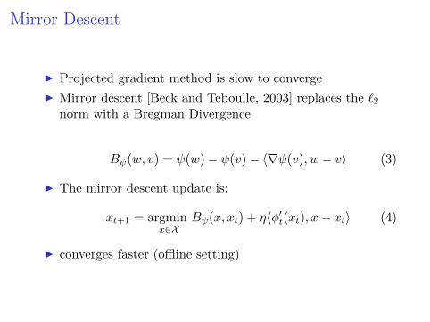
Mirror Descent
I Projected gradient method is slow to convergeI Mirror descent [Beck and Teboulle, 2003] replaces the `2
norm with a Bregman Divergence
Bψ(w, v) = ψ(w) − ψ(v) − 〈∇ψ(v), w − v〉 (3)
I The mirror descent update is:
xt+1 = argminx∈X
Bψ(x, xt) + η〈φ′t(xt), x− xt〉 (4)
I converges faster (offline setting)
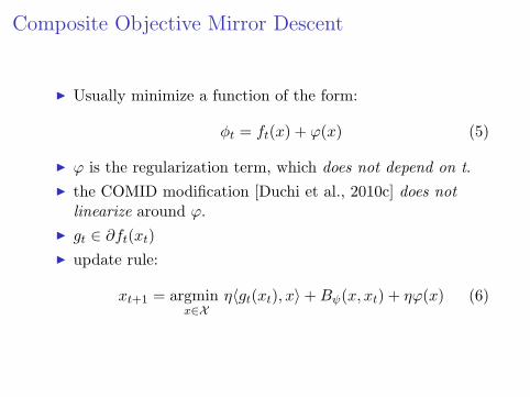
Composite Objective Mirror Descent
I Usually minimize a function of the form:
φt = ft(x) + ϕ(x) (5)
I ϕ is the regularization term, which does not depend on t.I the COMID modification [Duchi et al., 2010c] does not
linearize around ϕ.I gt ∈ ∂ft(xt)I update rule:
xt+1 = argminx∈X
η〈gt(xt), x〉 +Bψ(x, xt) + ηϕ(x) (6)
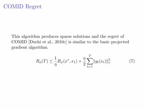
COMID Regret
This algorithm produces sparse solutions and the regret ofCOMID [Duchi et al., 2010c] is similar to the basic projectedgradient algorithm.
Rφ(T ) ≤ 1ηBψ(x∗, x1) +
η
2
T∑t=1
‖gt(xt)‖2∗ (7)

Outline
Online Convex Optimization
Composite Objective Mirror Descent
Regularized Dual Averaging
Adaptive Proximal Functions
Experiments
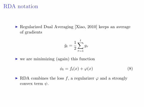
RDA notation
I Regularized Dual Averaging [Xiao, 2010] keeps an averageof gradients
gt =12
t∑τ=1
gτ
I we are minimizing (again) this function
φt = ft(x) + ϕ(x) (8)
I RDA combines the loss f , a regularizer ϕ and a stronglyconvex term ψ.
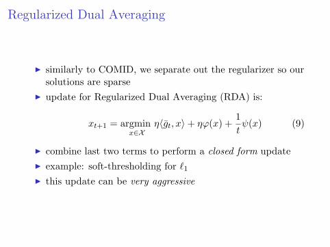
Regularized Dual Averaging
I similarly to COMID, we separate out the regularizer so oursolutions are sparse
I update for Regularized Dual Averaging (RDA) is:
xt+1 = argminx∈X
η〈gt, x〉 + ηϕ(x) +1tψ(x) (9)
I combine last two terms to perform a closed form updateI example: soft-thresholding for `1I this update can be very aggressive
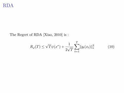
RDA
The Regret of RDA [Xiao, 2010] is :
Rϕ(T ) ≤√Tψ(x∗) +
12√T
T∑t=1
‖gt(xt)‖2∗ (10)

Outline
Online Convex Optimization
Composite Objective Mirror Descent
Regularized Dual Averaging
Adaptive Proximal Functions
Experiments
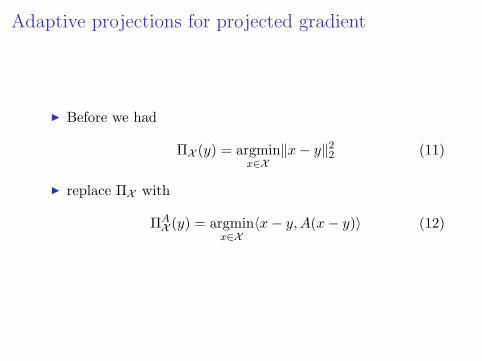
Adaptive projections for projected gradient
I Before we had
ΠX (y) = argminx∈X
‖x− y‖22 (11)
I replace ΠX with
ΠAX (y) = argmin
x∈X〈x− y,A(x− y)〉 (12)

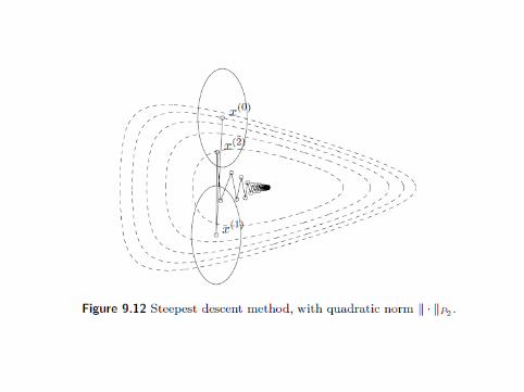
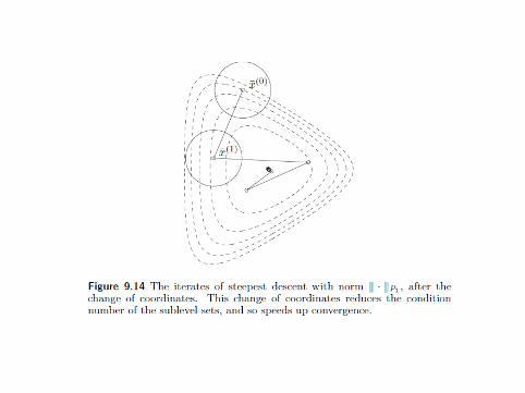
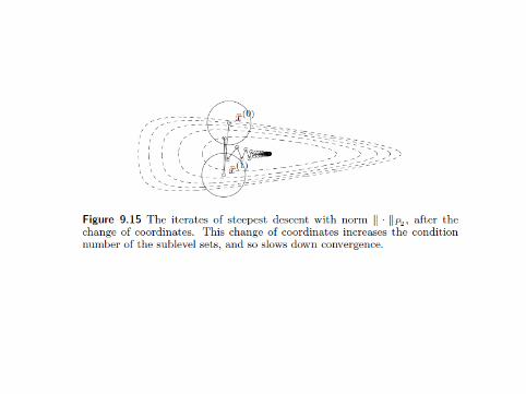
Why Change the Norm?
Slides are reproduced from [Boyd and Vandenberghe, 2004].
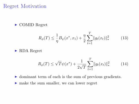
Regret Motivation
I COMID Regret
Rφ(T ) ≤ 1ηBψ(x∗, x1) +
η
2
T∑t=1
‖gt(xt)‖2∗ (13)
I RDA Regret
Rφ(T ) ≤√Tψ(x∗) +
12√T
T∑t=1
‖gt(xt)‖2∗ (14)
I dominant term of each is the sum of previous gradients.I make the sum smaller, we can lower regret
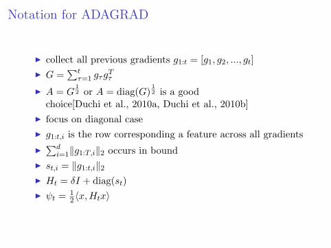
Notation for ADAGRAD
I collect all previous gradients g1:t = [g1, g2, ..., gt]I G =
∑tτ=1 gτg
Tτ
I A = G12 or A = diag(G)
12 is a good
choice[Duchi et al., 2010a, Duchi et al., 2010b]I focus on diagonal caseI g1:t,i is the row corresponding a feature across all gradientsI
∑di=1‖g1:T,i‖2 occurs in bound
I st,i = ‖g1:t,i‖2
I Ht = δI + diag(st)I ψt = 1
2〈x,Htx〉
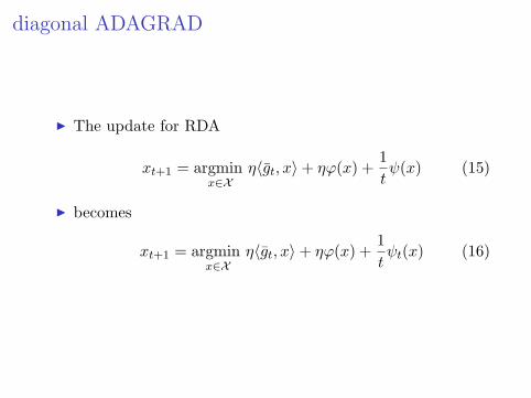
diagonal ADAGRAD
I The update for RDA
xt+1 = argminx∈X
η〈gt, x〉 + ηϕ(x) +1tψ(x) (15)
I becomes
xt+1 = argminx∈X
η〈gt, x〉 + ηϕ(x) +1tψt(x) (16)
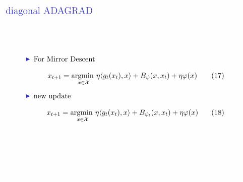
diagonal ADAGRAD
I For Mirror Descent
xt+1 = argminx∈X
η〈gt(xt), x〉 +Bψ(x, xt) + ηϕ(x) (17)
I new update
xt+1 = argminx∈X
η〈gt(xt), x〉 +Bψt(x, xt) + ηϕ(x) (18)
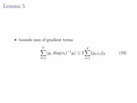
Lemma 5
I bounds sum of gradient terms
T∑t=1
〈gt,diag(st)−1gt〉 ≤ 2d∑i=1
‖g1:T,i‖2 (19)
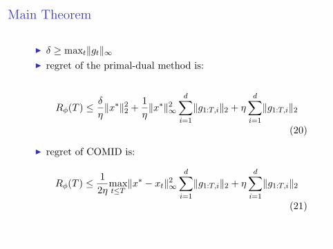
Main Theorem
I δ ≥ maxt‖gt‖∞I regret of the primal-dual method is:
Rφ(T ) ≤ δ
η‖x∗‖2
2 +1η‖x∗‖2
∞
d∑i=1
‖g1:T,i‖2 + η
d∑i=1
‖g1:T,i‖2
(20)
I regret of COMID is:
Rφ(T ) ≤ 12η
maxt≤T
‖x∗ − xt‖2∞
d∑i=1
‖g1:T,i‖2 + η
d∑i=1
‖g1:T,i‖2
(21)
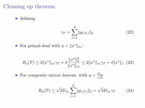
Cleaning up theorem
I defining
γT =d∑i=1
‖g1:T,i‖2 (22)
I For primal-dual with η = ‖x∗‖∞:
Rφ(T ) ≤ 2‖x∗‖∞γT + δ‖x∗‖2
2
‖x∗‖∞≤ 2‖x∗‖∞γT + δ‖x∗‖1 (23)
I For composite mirror descent, with η = D∞√2
Rφ(T ) ≤√
2D∞
d∑i=1
‖g1:T,i‖2 =√
2D∞γT (24)

Outline
Online Convex Optimization
Composite Objective Mirror Descent
Regularized Dual Averaging
Adaptive Proximal Functions
Experiments
Experiments
I comparisons are to Passive Aggressive and AROWalgorithms
I these are adaptive, but arise from mistake boundsI FOBOS is an earlier non-adaptive algorithm
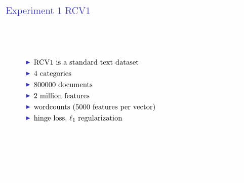
Experiment 1 RCV1
I RCV1 is a standard text datasetI 4 categoriesI 800000 documentsI 2 million featuresI wordcounts (5000 features per vector)I hinge loss, `1 regularization
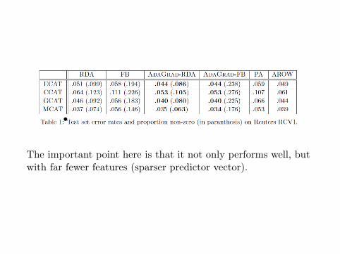
The important point here is that it not only performs well, butwith far fewer features (sparser predictor vector).
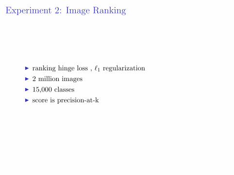
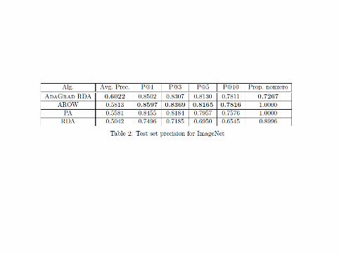
Experiment 2: Image Ranking
I ranking hinge loss , `1 regularizationI 2 million imagesI 15,000 classesI score is precision-at-k
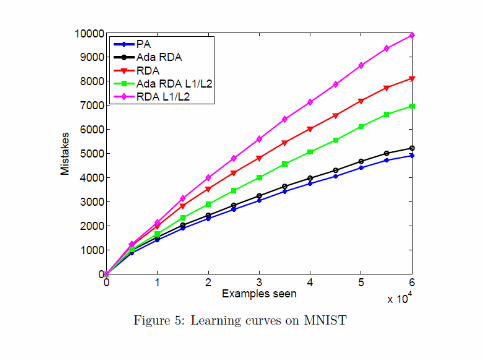
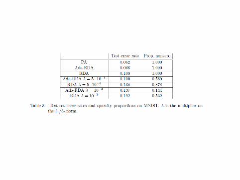
Experiment 3: MNIST
I MNIST is standard digit recognition taskI 60,000 examplesI 30,000 featuresI classifier is a Gaussian kernel machine
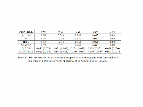
Experiment 4 Census
I UCI dataset, predict income level from features > $50000I 4001 features, binary featuresI 199,523 training samples
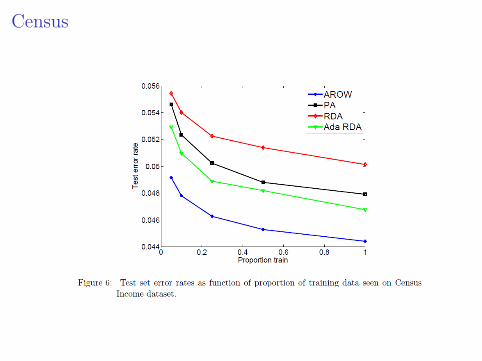
Census
Conclusions
I RDA and COMID exploit regularizer betterI can derive adaptive version of these algorithmsI can achieve low regretI good predictive accuracyI better sparsity than comparable algorithms
Not Covered
I lowering regret for strongly convex functionsI regret bounds and algorithm for full matrix algorithmI implementation details (Section 6 of tech report).
Abernethy, J., Bartlett, P., Rakhlin, A., and Tewari, A.(2008).Optimal strategies and minimax lower bounds for onlineconvex games.In Proceedings of the Nineteenth Annual Conference onComputational Learning Theory.
Beck, A. and Teboulle, M. (2003).Mirror descent and nonlinear projected subgradientmethods for convex optimization.Operations Research Letters, 31(3):167–175.
Boyd, S. and Vandenberghe, L. (2004).Convex optimization.Cambridge Univ Pr.
Duchi, J., Hazan, E., and Singer, Y. (2010a).Adaptive subgradient methods for online learning andstochastic optimization.UC Berkeley EECS Technical Report, 24:1–41.
Duchi, J., Hazan, E., and Singer, Y. (2010b).Adaptive subgradient methods for online learning andstochastic optimization .In Proceedings of the Twenty Third Annual Conference onComputational Learning Theory, number 1.
Duchi, J., Shalev-Shwartz, S., Singer, Y., Tewari, A., andChicago, T. (2010c).Composite objective mirror descent.In Proceedings of the Twenty Third Annual Conference onComputational Learning Theory, number 1.
Xiao, L. (2010).Dual Averaging Methods for Regularized StochasticLearning and Online Optimization.Journal of Machine Learning Research, 11:2543–2596.
Zinkevich, M. (2003).Online Convex Programming and Generalized InfinitesimalGradient Ascent.

In International Conference on Machine Learning, pages421–422.