Air Bearing Optimization

Jennifer Egolf Sumanth Swaminathan

Kyle Spence

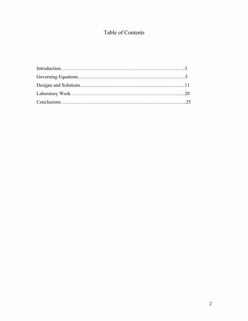
Table of Contents

Introduction…………………………………………………………………..3

Governing Equations…………………………………………………………5

Designs and Solutions………………………………………………………..11

Laboratory Work……………………………………………………………..20

Conclusions…………………………………………………………………...25

2

Introduction

Air bearings are non-contact bearings that utilize a thin film of pressurized air to

provide a frictionless interface between two surfaces. Applications of air bearings

include precision machine tools, semiconductor wafer-processing machines, and other

clean-room, high-speed, and precision positioning environments. The non-contact

principles of an air bearing provide clear advantages over traditional bearings since

problems such as wear are eliminated.

Figure A. Air bearing vs. roller bearing. It is noted the type of fluid bearing

examined in this document is of planar orientation rather than the rotational bearing

shown here.

The goal for this project is to optimize the lift of a planar circular air bearing.

Optimizing the bearing will maximize the load that the bearing can accommodate at an

applied pressure. The solution to this problem is valuable because it will increase the

efficiency of air bearings.

We will begin the optimization by investigating the effect of various patterns

etched onto the bottom surface of the bearing. We will start by taking a circular air

bearing of fixed dimensions with no etchings and suspending it over a fixed volume of

incompressible, constant density air. The bearing hovers over a flat surface due to

pressurized airflow introduced to the system. A simplified version of the Reynolds

equation will be used to develop a relationship between pressure and the gap height

between the bearing and the inlet surface. The height will be a function of the radius.

Ultimately, a design that produces optimum lift will be identified. We will also use

Newton’s Second Law to find a relationship between the pressure and the mass on top of

the bearing.

3

This document will build on theories of lubrication and fluid mechanics to

develop optimal designs for an air bearing. Important equations that define our problem

were identified through research of previous work in the lubrication field. An annotated

bibliography is found in appendix A. Key issues for this problem will be defining all the

parameters for optimization, defining the physical bounds of the system’s inlet pressure,

and developing a method for verification of models. We plan to use numerical methods

to observe how pressure is affected by different functions of gap height.

The problem will focus on circular air bearings. Figure B illustrates the basic

schematics for a circular air bearing. The bearing floats above the surface due to air

pressure through the gap height, h. The air beneath the bearing acts as a fluid and creates

a lubricant film. For this reason, equations of lubrication theory are relevant to this

problem. The goal of the project is to maximize the total pressure force under the air

bearing by creating channels that “capture” the higher inlet pressure.

Figure B: General schematics for an air bearing. The air bearing we will be discussing is

of planar orientation, similar to the idea of an air hockey puck hovering over the surface

of the table.

4

Governing Equations

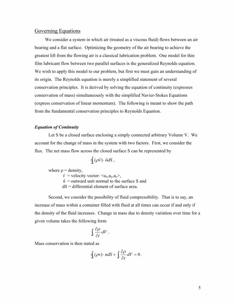
We consider a system in which air (treated as a viscous fluid) flows between an air

bearing and a flat surface. Optimizing the geometry of the air bearing to achieve the

greatest lift from the flowing air is a classical lubrication problem. One model for thin

film lubricant flow between two parallel surfaces is the generalized Reynolds equation.

We wish to apply this model to our problem, but first we must gain an understanding of

its origin. The Reynolds equation is merely a simplified statement of several

conservation principles. It is derived by solving the equation of continuity (expresses

conservation of mass) simultaneously with the simplified Navier-Stokes Equations

(express conservation of linear momentum). The following is meant to show the path

from the fundamental conservation principles to Reynolds Equation.

Equation of Continuity

Let S be a closed surface enclosing a simply connected arbitrary Volume V. We

account for the change of mass in the system with two factors. First, we consider the

flux. The net mass flow across the closed surface S can be represented by

dSnvS

ˆ)( ⋅∫rρ ,

where ρ = density, v = velocity vector: <ur

x,uy,uz>, n = outward unit normal to the surface S and ˆ dS = differential element of surface area. Second, we consider the possibility of fluid compressibility. That is to say, an

increase of mass within a container filled with fluid at all times can occur if and only if

the density of the fluid increases. Change in mass due to density variation over time for a

given volume takes the following form

∫ ∂∂

VdV

tρ .

Mass conservation is then stated as

0)( =∂∂

+⋅ ∫∫ VSdV

tndSv ρρ .

5

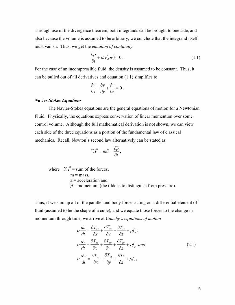
Through use of the divergence theorem, both integrands can be brought to one side, and

also because the volume is assumed to be arbitrary, we conclude that the integrand itself

must vanish. Thus, we get the equation of continuity

( ) 0=+∂∂ vdiv

tρρ . (1.1)

For the case of an incompressible fluid, the density is assumed to be constant. Thus, it

can be pulled out of all derivatives and equation (1.1) simplifies to

0=∂∂

+∂∂

+∂∂

zv

yv

xv .

Navier Stokes Equations

The Navier-Stokes equations are the general equations of motion for a Newtonian

Fluid. Physically, the equations express conservation of linear momentum over some

control volume. Although the full mathematical derivation is not shown, we can view

each side of the three equations as a portion of the fundamental law of classical

mechanics. Recall, Newton’s second law alternatively can be stated as

tpamF

∂∂

==∑~rr

,

where = sum of the forces, F

r∑

m = mass, a = acceleration and p~ = momentum (the tilde is to distinguish from pressure).

Thus, if we sum up all of the parallel and body forces acting on a differential element of

fluid (assumed to be the shape of a cube), and we equate those forces to the change in

momentum through time, we arrive at Cauchy’s equations of motion

,

,

,

zyzxz

yzyyyxy

xzxyxxx

fz

Tzy

Tx

Tdtdw

andfz

Ty

Tx

Tdtdv

fz

Ty

Tx

Tdtdu

ρρ

ρρ

ρρ

+∂

∂+

∂

∂+

∂∂

=

+∂

∂+

∂

∂+

∂

∂=

+∂

∂+

∂

∂+

∂∂

=

(2.1)

6

where: T = stress, ρ = density, u = velocity in x-direction, v = velocity in y-direction, w = velocity in z-direction and f = body forces. We then relate stress forces to the velocity by Newton’s viscosity relation which states

j

iji x

uT

∂∂

= µ, .

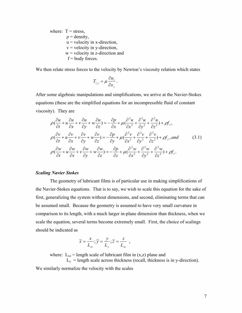
After some algebraic manipulations and simplifications, we arrive at the Navier-Stokes

equations (these are the simplified equations for an incompressible fluid of constant

viscosity). They are

.)()(

,)()(

,)()(

2

2

2

2

2

2

2

2

2

2

2

2

2

2

2

2

2

2

z

y

x

fzw

yw

xw

zp

zww

ywv

xwu

tw

andfzv

yv

xv

yp

zvw

yvv

xvu

tv

fzu

yu

xu

xp

zuw

yuv

xuu

tu

ρµρ

ρµρ

ρµρ

+∂∂

+∂∂

+∂∂

+∂∂

−=∂∂

+∂∂

+∂∂

+∂∂

+∂∂

+∂∂

+∂∂

+∂∂

−=∂∂

+∂∂

+∂∂

+∂∂

+∂∂

+∂∂

+∂∂

+∂∂

−=∂∂

+∂∂

+∂∂

+∂∂

(3.1)

Scaling Navier Stokes

The geometry of lubricant films is of particular use in making simplifications of

the Navier-Stokes equations. That is to say, we wish to scale this equation for the sake of

first, generalizing the system without dimensions, and second, eliminating terms that can

be assumed small. Because the geometry is assumed to have very small curvature in

comparison to its length, with a much larger in-plane dimension than thickness, when we

scale the equation, several terms become extremely small. First, the choice of scalings

should be indicated as

xzyxz Lzz

Lyy

Lxx === ~;~;~ ,

where: Lxz = length scale of lubricant film in (x,z) plane and Ly = length scale across thickness (recall, thickness is in y-direction).

We similarly normalize the velocity with the scales

7

***

~;~;~Uww

Vvv

Uuu === .

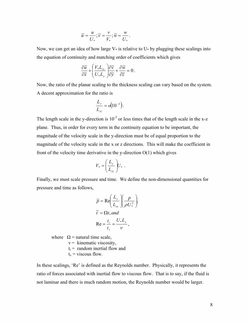
Now, we can get an idea of how large V* is relative to U* by plugging these scalings into

the equation of continuity and matching order of coefficients which gives

0~~

~~

~~

*

* =∂∂

+∂∂

+

∂∂

zw

yv

LULV

xu

y

xz .

Now, the ratio of the planar scaling to the thickness scaling can vary based on the system.

A decent approximation for the ratio is

( )310−= oLL

xz

y .

The length scale in the y-direction is 10-3 or less times that of the length scale in the x-z

plane. Thus, in order for every term in the continuity equation to be important, the

magnitude of the velocity scale in the y-direction must be of equal proportion to the

magnitude of the velocity scale in the x or z directions. This will make the coefficient in

front of the velocity time derivative in the y-direction O(1) which gives

** ULL

xz

y

=V .

Finally, we must scale pressure and time. We define the non-dimensional quantities for

pressure and time as follows,

,Re

,~

,Re~

*

2*

ν

ρ

y

v

i

xz

y

LUtt

andtt

Up

LL

p

==

Ω=

=

where Ω = natural time scale, ν = kinematic viscosity, ti = random inertial flow and tv = viscous flow. In these scalings, ‘Re’ is defined as the Reynolds number. Physically, it represents the

ratio of forces associated with inertial flow to viscous flow. That is to say, if the fluid is

not laminar and there is much random motion, the Reynolds number would be larger.

8

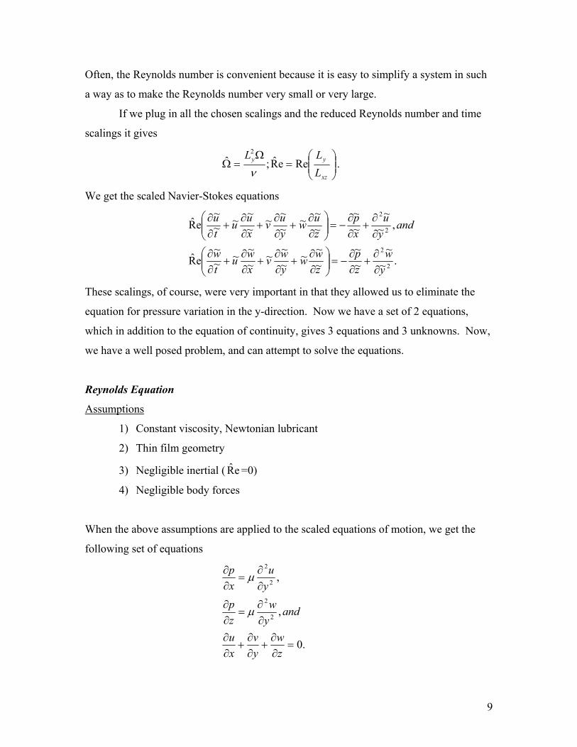
Often, the Reynolds number is convenient because it is easy to simplify a system in such

a way as to make the Reynolds number very small or very large.

If we plug in all the chosen scalings and the reduced Reynolds number and time

scalings it gives

=

Ω=Ω

xz

yy

LLL

ReeR;ˆ2

ν.

We get the scaled Navier-Stokes equations

.~

~~~

~~~

~~~

~~~

~~

eR

,~~

~~

~~~

~~~

~~~

~~

eR

2

2

2

2

yw

zp

zww

ywv

xwu

tw

andyu

xp

zuw

yuv

xuu

tu

∂∂

+∂∂

−=

∂∂

+∂∂

+∂∂

+∂∂

∂∂

+∂∂

−=

∂∂

+∂∂

+∂∂

+∂∂

These scalings, of course, were very important in that they allowed us to eliminate the

equation for pressure variation in the y-direction. Now we have a set of 2 equations,

which in addition to the equation of continuity, gives 3 equations and 3 unknowns. Now,

we have a well posed problem, and can attempt to solve the equations.

Reynolds Equation

Assumptions

1) Constant viscosity, Newtonian lubricant

2) Thin film geometry

3) Negligible inertial ( =0) eR

4) Negligible body forces

When the above assumptions are applied to the scaled equations of motion, we get the

following set of equations

.0

,

,

2

2

2

2

=∂∂

+∂∂

+∂∂

∂∂

=∂∂

∂∂

=∂∂

zw

yv

xu

andyw

zp

yu

xp

µ

µ

9

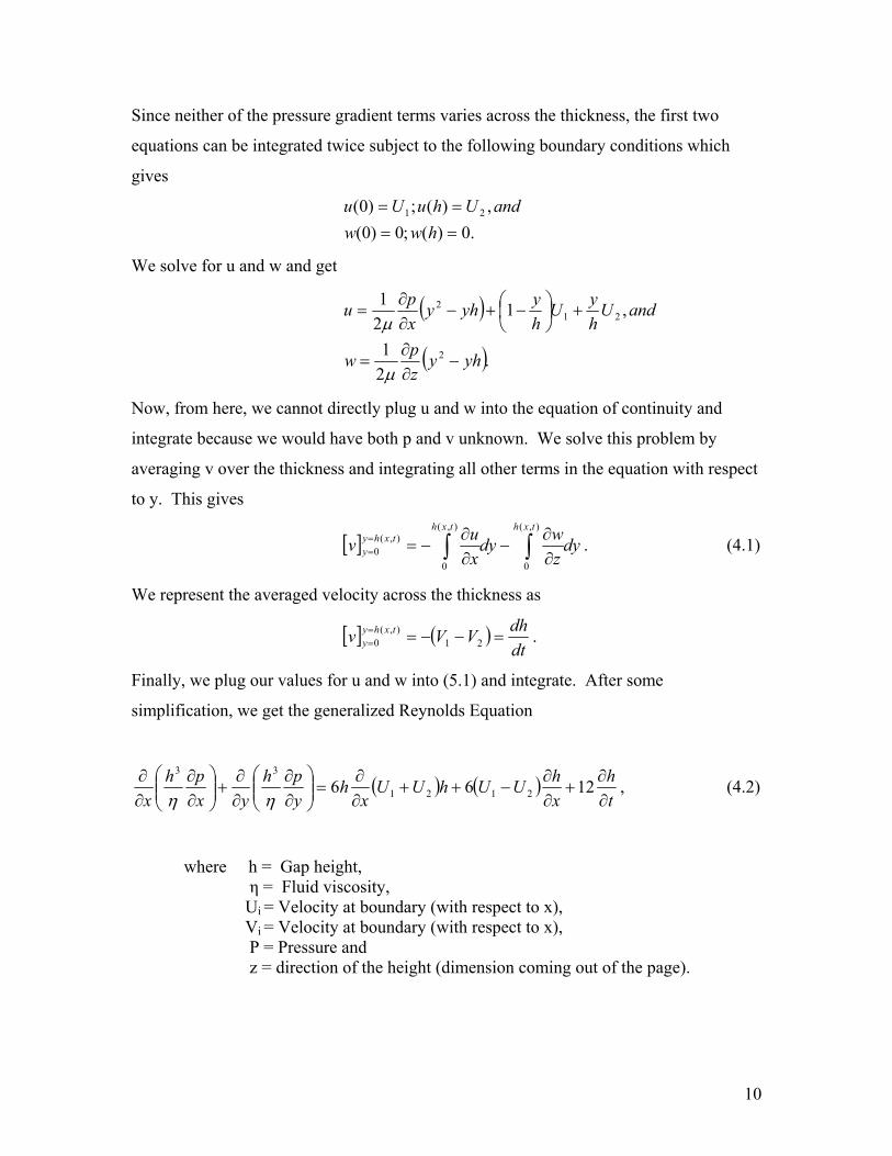
Since neither of the pressure gradient terms varies across the thickness, the first two

equations can be integrated twice subject to the following boundary conditions which

gives

.0)(;0)0(

,)(;)0( 21

====

hwwandUhuUu

We solve for u and w and get

( )

( ).21

,121

2

212

yhyzpw

andUhyU

hyyhy

xpu

−∂∂

=

+

−+−

∂∂

=

µ

µ

Now, from here, we cannot directly plug u and w into the equation of continuity and

integrate because we would have both p and v unknown. We solve this problem by

averaging v over the thickness and integrating all other terms in the equation with respect

to y. This gives

[ ] dyzwdy

xuv

txhtxhtxhy

y ∫∫ ∂∂

−∂∂

−===

),(

0

),(

0

),(0 . (4.1)

We represent the averaged velocity across the thickness as

[ ] ( )dtdhVVv txhy

y =−−=== 21

),(0 .

Finally, we plug our values for u and w into (5.1) and integrate. After some

simplification, we get the generalized Reynolds Equation

( ) ( )th

xhUUhUU

xh

yph

yxph

x ∂∂

+∂∂

−++∂∂

=

∂∂

∂∂

+

∂∂

∂∂ 1266 2121

33

ηη, (4.2)

where h = Gap height, η = Fluid viscosity, Ui = Velocity at boundary (with respect to x), Vi = Velocity at boundary (with respect to x), P = Pressure and z = direction of the height (dimension coming out of the page).

10

Reynolds equation in lubricant pressure is the mathematical statement of the

classical theory of lubrication. Physically, it can be thought of as an expression of

conservation principles for a system made up of lubricant flow between two parallel

surfaces. The terms on the left-hand side of the equation represent flow due to pressure

gradients across the domain, while the terms on the right hand side represent flows

induced by motions of the bounding surfaces and shear induced flow by the sliding

velocities U and V. For our purposes, we assume no such motions of the bounding

surfaces, and also no time dependence.

Designs & Solutions Manipulation of the Reynolds equation is quite difficult without knowledge of the

geometry of the system. The geometry of the system cannot be achieved without a

known design for the bearing. Thus, we will not be optimizing the design of the bearing

subject to the Reynolds equation; rather we will be using the Reynolds equation to find

the lift coefficient once a design has been chosen. The hope is that we can study and

optimize the lift coefficient once an analytical expression for it is found through the

Reynolds equation.

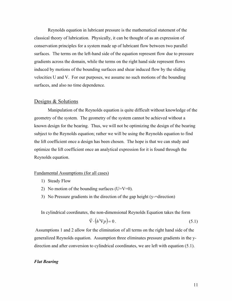
Fundamental Assumptions (for all cases)

1) Steady Flow

2) No motion of the bounding surfaces (U=V=0).

3) No Pressure gradients in the direction of the gap height (y-=direction)

In cylindrical coordinates, the non-dimensional Reynolds Equation takes the form

( ) 03 =∇⋅∇ phr

. (5.1)

Assumptions 1 and 2 allow for the elimination of all terms on the right hand side of the

generalized Reynolds equation. Assumption three eliminates pressure gradients in the y-

direction and after conversion to cylindrical coordinates, we are left with equation (5.1).

Flat Bearing

11

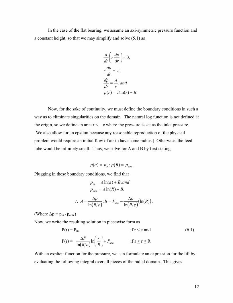
In the case of the flat bearing, we assume an axi-symmetric pressure function and

a constant height, so that we may simplify and solve (5.1) as

.)ln()(

,

,

,0

BrArp

andrA

drdp

Adrdp

drdpr

drd

+=

=

=

=

r

Now, for the sake of continuity, we must define the boundary conditions in such a

way as to eliminate singularities on the domain. The natural log function is not defined at

the origin, so we define an area r < ε where the pressure is set as the inlet pressure.

[We also allow for an epsilon because any reasonable reproduction of the physical

problem would require an initial flow of air to have some radius.] Otherwise, the feed

tube would be infinitely small. Thus, we solve for A and B by first stating

atmin pRppp == )(;)(ε .

Plugging in these boundary conditions, we find that

.)ln(

,)ln(BRApandBAp

atm

in

+=+= ε

( ) ( ) ( ))ln(ln

;ln

RRpPB

RpA atm εε

∆−=

∆=∴ .

(Where ∆p = pin - patm.)

Now, we write the resulting solution in piecewise form as

P(r) = Pin if r < ε and (6.1)

P(r) = ( ) atmPRr

RP

+

ln

ln ε∆ if ε < r < R.

With an explicit function for the pressure, we can formulate an expression for the lift by

evaluating the following integral over all pieces of the radial domain. This gives

12

. ( )∫∫Ω

−= dAprpL atm)(

For our case we have

( )

( ) ( ).ln2

1

,lnln

)(

22

2

0

2

0 0

εε

π

θε

θπ

ε

π ε

−∆

=

∆

+∆= ∫ ∫∫ ∫

RRpL

andrdrdRr

RprdrdpL

R

(6.2)

Finally, we relate pressure to the amount of applied weight by concluding that in

order for the bearing to hover at a constant height, the lift force associated with the

applied pressure must equal the force of weight pushing down. Newton’s second law

says: F=ma. Thus, we conclude that L=mg (for g = gravitational force). Substituting this

equation into our expression for the lift and solving for ∆P we find

( ) MR

Rgp)(

ln222 επε

−=∆ . (6.3)

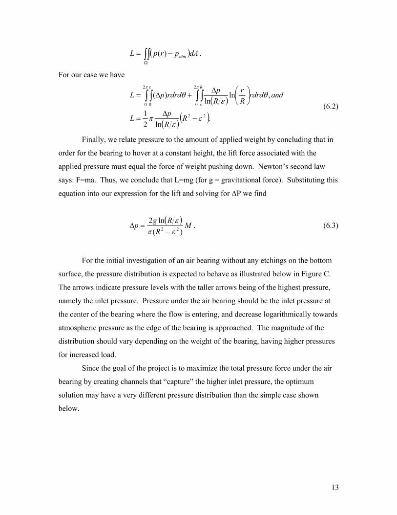
For the initial investigation of an air bearing without any etchings on the bottom

surface, the pressure distribution is expected to behave as illustrated below in Figure C.

The arrows indicate pressure levels with the taller arrows being of the highest pressure,

namely the inlet pressure. Pressure under the air bearing should be the inlet pressure at

the center of the bearing where the flow is entering, and decrease logarithmically towards

atmospheric pressure as the edge of the bearing is approached. The magnitude of the

distribution should vary depending on the weight of the bearing, having higher pressures

for increased load.

Since the goal of the project is to maximize the total pressure force under the air

bearing by creating channels that “capture” the higher inlet pressure, the optimum

solution may have a very different pressure distribution than the simple case shown

below.

13

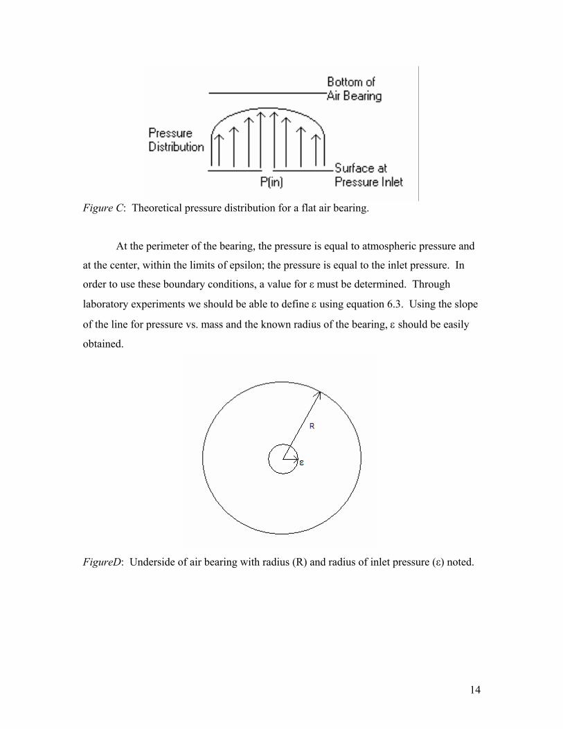
Figure C: Theoretical pressure distribution for a flat air bearing.

At the perimeter of the bearing, the pressure is equal to atmospheric pressure and

at the center, within the limits of epsilon; the pressure is equal to the inlet pressure. In

order to use these boundary conditions, a value for ε must be determined. Through

laboratory experiments we should be able to define ε using equation 6.3. Using the slope

of the line for pressure vs. mass and the known radius of the bearing, ε should be easily

obtained.

FigureD: Underside of air bearing with radius (R) and radius of inlet pressure (ε) noted.

14

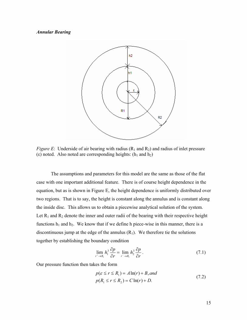
Annular Bearing

Figure E: Underside of air bearing with radius (R1 and R2) and radius of inlet pressure (ε) noted. Also noted are corresponding heights: (h1 and h2)

The assumptions and parameters for this model are the same as those of the flat

case with one important additional feature. There is of course height dependence in the

equation, but as is shown in Figure E, the height dependence is uniformly distributed over

two regions. That is to say, the height is constant along the annulus and is constant along

the inside disc. This allows us to obtain a piecewise analytical solution of the system.

Let R1 and R2 denote the inner and outer radii of the bearing with their respective height

functions h1 and h2. We know that if we define h piece-wise in this manner, there is a

discontinuous jump at the edge of the annulus (R1). We therefore tie the solutions

together by establishing the boundary condition

rph

rph

RrRr ∂∂

=∂∂

→→ −+

32

31

11

limlim . (7.1)

Our pressure function then takes the form

.)ln()(

,)ln()(

21

1

DrCRrRpandBrARrp

+=≤≤+=≤≤ε

(7.2)

15

Just as before, we let the inlet pressure be constant over a disc of radius ε(this disc

representing the area covered by the pipe head), and we let the pressure at the boundary

(r=R2) be atmospheric pressure. Plugging these boundary conditions into (7.2) and then

plugging that result into (7.1), we find that

,)ln(

,)ln(

2 atm

in

pDRCpBA=+

=+ε (7.3)

.

,

,

,

3

1

2

3

1

2

31

1

32

1

CAH

andhhH

AChh

hRAh

RC

=

=

=

=

Conditions of continuity across the underside of the bearing ensuring that there are no

singularities at r = R1 imply that

and).ln()ln()ln(

)ln()ln(

211

11

RCpRCBRA

DRCBRA

atm −+=+

+=+

We can then solve for the four coefficients which are

).ln(

,

ln

),ln(

,

ln

2

2

1

2

1

3

3

13

3

13

RCpD

and

R

R

PC

ApBR

R

PHA

atm

H

H

in

H

H

−=

∆

=

−=

∆

=

−

−−

−

−−

ε

ε

ε

Using these coefficients, we have a piece-wise analytical solution for p(r). That solution

is

16

.ln

ln

)(

,ln

ln

)(

,)(

2

)(2

)1(1

21

)(2

)1(1

3

1

3

3

3

3

atm

H

H

in

H

H

in

pRr

RR

pRrRp

andpr

RR

pHRrp

prp

+

∆

=≤≤

+

∆

=≤≤

=<

−

−

−

−

−

−

ε

εεε

ε

(7.4)

Integrating piece-wise and summing as with the flat bearing, we find that

( )[ ]221

22

3

)1(21

1

ln2

3

3ε

ε

π−+−

∆

=

−RRH

RR

pL

H

H. (7.5)

Finally, letting L = mg under the assumption that at equilibrium, the

bearing must exactly counteract the applied mass and its own mass, we find our

expression for the pressure drop under the bearing as

( )[ ]MRRH

RRg

pH

H

221

22

3

)1(21

1

ln2 3

3

επε

−+−

=∆

−

. (7.6)

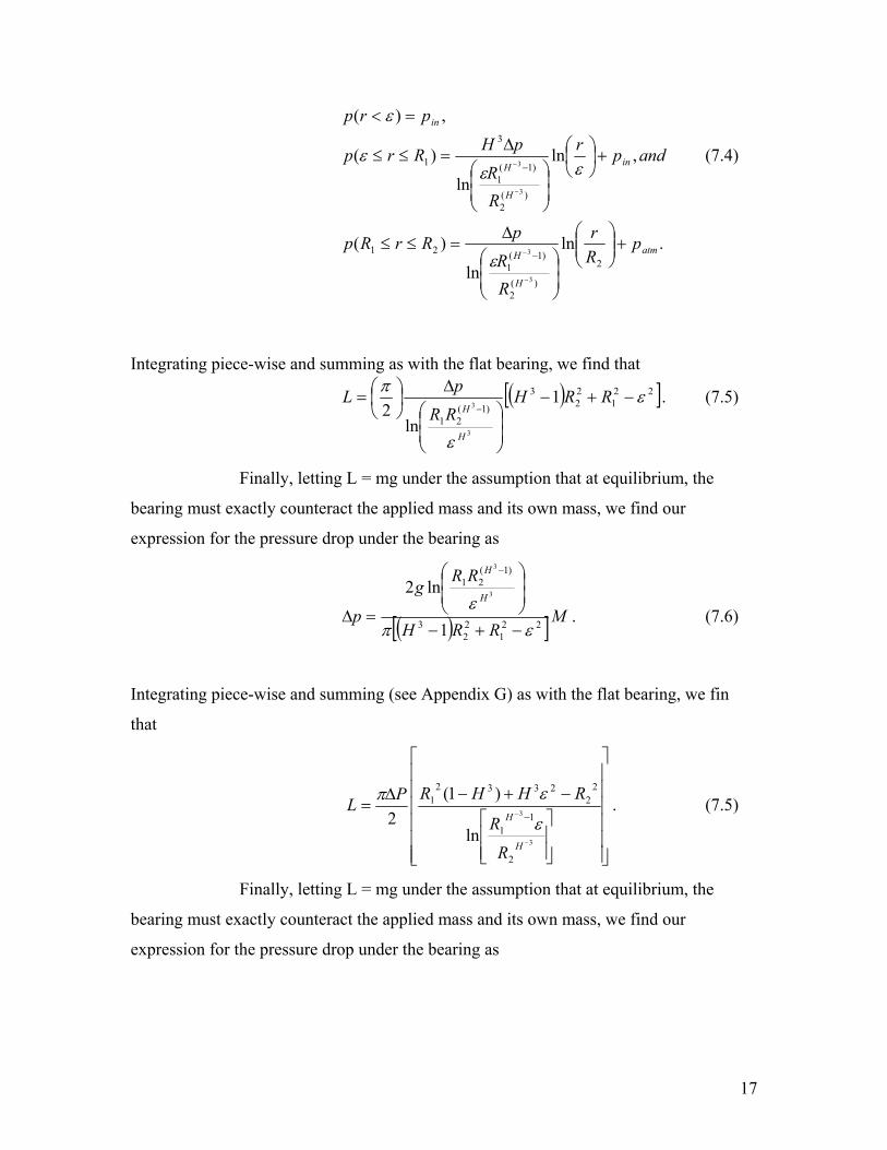
Integrating piece-wise and summing (see Appendix G) as with the flat bearing, we fin

that

−+−∆

−

− −

3

3

2

11

22

23321

ln

)1(2

H

H

R

R

RHHRP

ε

επ=L . (7.5)

Finally, letting L = mg under the assumption that at equilibrium, the

bearing must exactly counteract the applied mass and its own mass, we find our

expression for the pressure drop under the bearing as

17

−+−

=∆−

− −

22

23321

2

11

)1(

ln2

3

3

RHHRR

R

MgpH

H

ε

ε

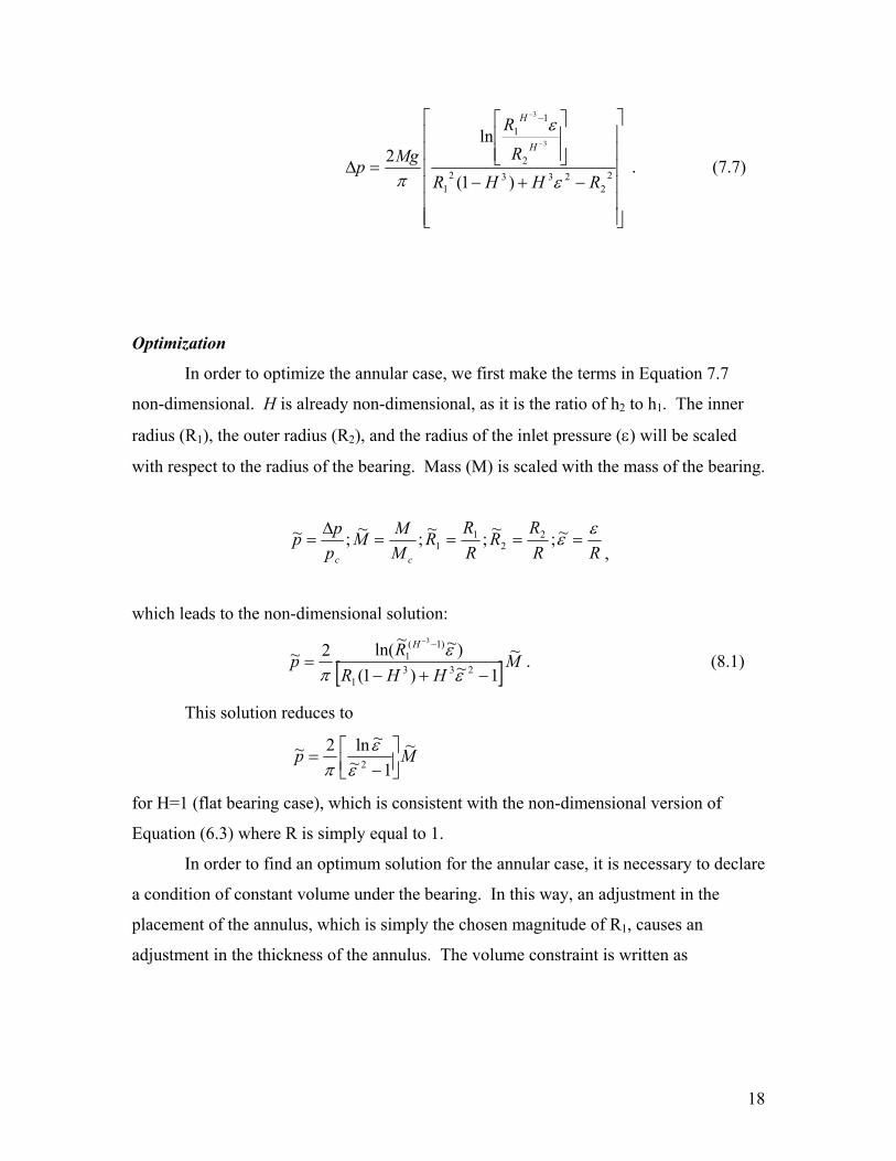
π . (7.7)

Optimization

In order to optimize the annular case, we first make the terms in Equation 7.7

non-dimensional. H is already non-dimensional, as it is the ratio of h2 to h1. The inner

radius (R1), the outer radius (R2), and the radius of the inlet pressure (ε) will be scaled

with respect to the radius of the bearing. Mass (M) is scaled with the mass of the bearing.

RRRR

RRR

MMM

ppp

cc

εε ====∆

= ~;~;~;~;~ 22

11 ,

which leads to the non-dimensional solution:

[ ]MHHR

Rp

H ~1~)1(

)~~ln(2~233

1

)1(1

3

−+−=

−−

εε

π. (8.1)

This solution reduces to

Mp ~1~

~ln2~2

−=

εε

π

for H=1 (flat bearing case), which is consistent with the non-dimensional version of

Equation (6.3) where R is simply equal to 1.

In order to find an optimum solution for the annular case, it is necessary to declare

a condition of constant volume under the bearing. In this way, an adjustment in the

placement of the annulus, which is simply the chosen magnitude of R1, causes an

adjustment in the thickness of the annulus. The volume constraint is written as

18

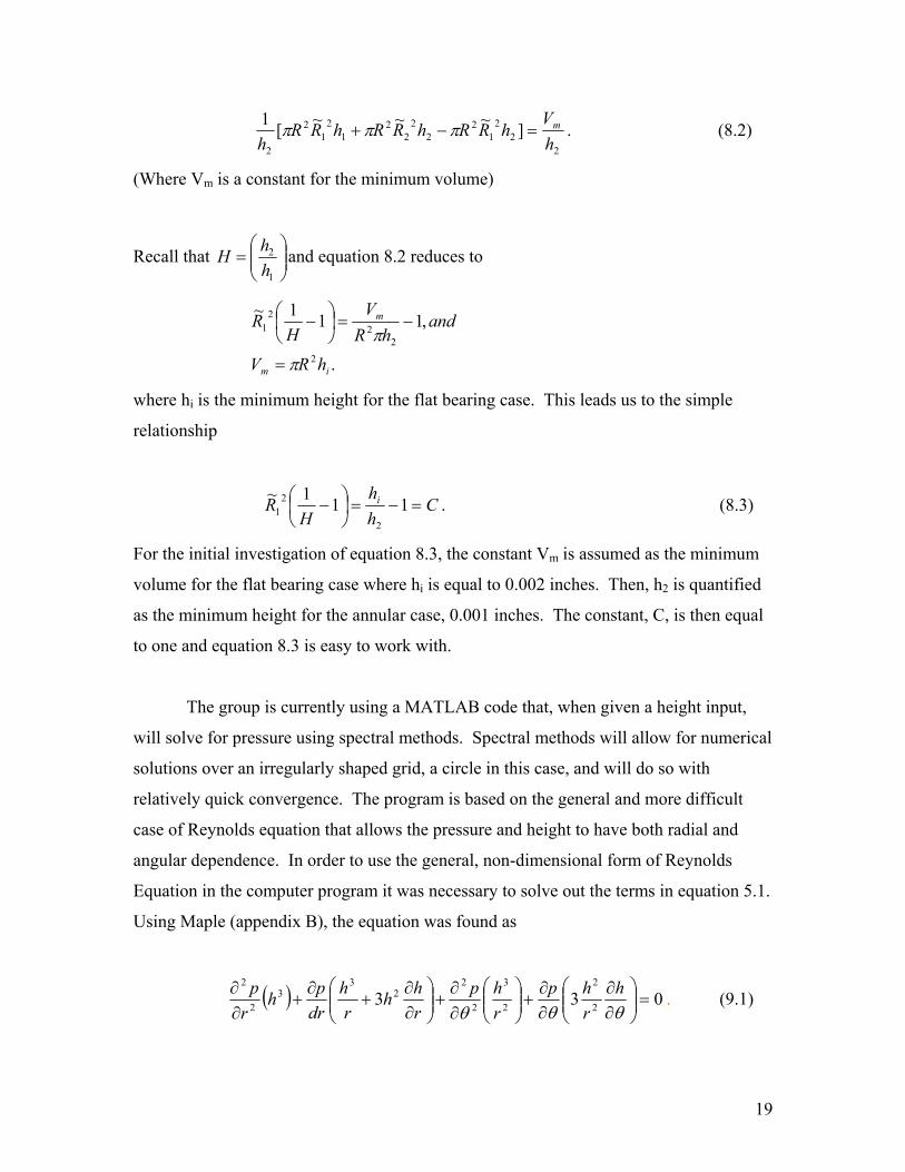
2

22

12

22

22

12

12

2

]~~~[1hV

hRRhRRhRRh

m=−+ πππ . (8.2)

(Where Vm is a constant for the minimum volume)

Recall that

=

1

2

hhH and equation 8.2 reduces to

.

,111~

22

22

1

im

m

hRV

andhR

VH

R

π

π

=

−=

−

where hi is the minimum height for the flat bearing case. This leads us to the simple

relationship

Chh

HR i =−=

− 111~

2

21 . (8.3)

For the initial investigation of equation 8.3, the constant Vm is assumed as the minimum

volume for the flat bearing case where hi is equal to 0.002 inches. Then, h2 is quantified

as the minimum height for the annular case, 0.001 inches. The constant, C, is then equal

to one and equation 8.3 is easy to work with.

The group is currently using a MATLAB code that, when given a height input,

will solve for pressure using spectral methods. Spectral methods will allow for numerical

solutions over an irregularly shaped grid, a circle in this case, and will do so with

relatively quick convergence. The program is based on the general and more difficult

case of Reynolds equation that allows the pressure and height to have both radial and

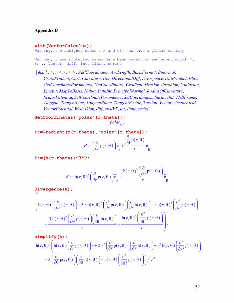
angular dependence. In order to use the general, non-dimensional form of Reynolds

Equation in the computer program it was necessary to solve out the terms in equation 5.1.

Using Maple (appendix B), the equation was found as

( ) 033 2

2

2

3

2

22

33

2

2

=

∂∂

∂∂

+

∂∂

+

∂∂

+∂

+∂∂

θθθh

rhp

rhp

rhh

rh

drph

rp . (9.1)

19

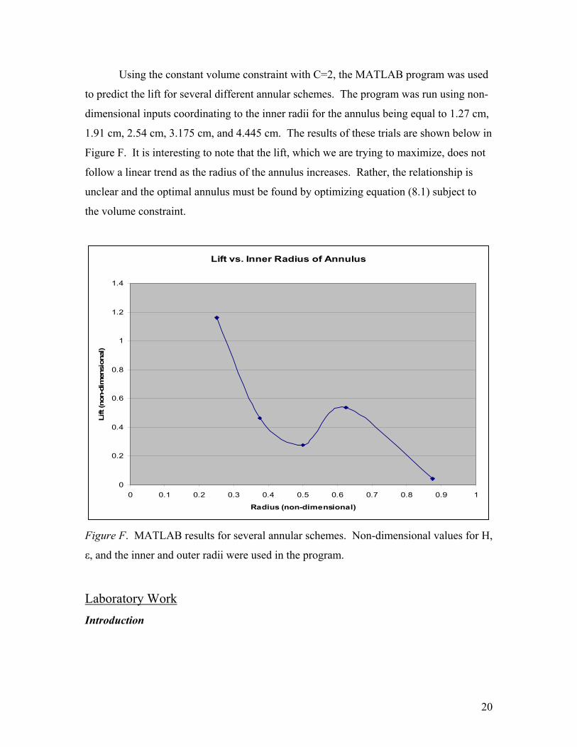
Using the constant volume constraint with C=2, the MATLAB program was used

to predict the lift for several different annular schemes. The program was run using non-

dimensional inputs coordinating to the inner radii for the annulus being equal to 1.27 cm,

1.91 cm, 2.54 cm, 3.175 cm, and 4.445 cm. The results of these trials are shown below in

Figure F. It is interesting to note that the lift, which we are trying to maximize, does not

follow a linear trend as the radius of the annulus increases. Rather, the relationship is

unclear and the optimal annulus must be found by optimizing equation (8.1) subject to

the volume constraint.

Lift vs. Inner Radius of Annulus

0

0.2

0.4

0.6

0.8

1

1.2

1.4

0 0.1 0.2 0.3 0.4 0.5 0.6 0.7 0.8 0.9 1

Radius (non-dimensional)

Lift

(non

-dim

ensi

onal

)

Figure F. MATLAB results for several annular schemes. Non-dimensional values for H,

ε, and the inner and outer radii were used in the program.

Laboratory Work Introduction

20

The purpose of our laboratory experiments is to give us a better understanding of

our problem and to assist us in solving it. In the experiments we test various bearings

with different etching patterns. We show that there is a linear relationship between

pressure and applied mass for any etching carved into the bottom of the air bearing. This

allows us to find better designs and predict the pressure for certain masses applied to an

air bearing. Essentially, the shallower the slope of the pressure vs. applied mass plot, the

better the design.

We ran into some difficulties when we first started our lab experiments. The

epoxy bond that held the pressure fitting to the flat surface leaked and then broke off.

This required that we refit our apparatus before we could proceed with our experiments.

Procedure

A pressure fitting forces air through a hole in a glass disk upon which the air

bearing floats. A pressure sensor is attached to the pressure valve and provides a reading

of the pressure under the bearing. Different bearing designs are made using four and six

inch glass bearings with shim stock applied to the bottom surfaces to simulate etchings.

The bearings are placed onto the pressure feeding surface and several small

masses are applied all at once. Then the pressure valve is opened and the data recording

program is run. The small masses are then removed one by one allowing a period of time

to pass between each loading case. Once all the masses are removed and data for the case

of no applied mass is recorded, a different bearing is then tested with the same masses

and same flow rate as was just used. This is repeated for all the bearings to be tested at

that time.

Results

Experiment 1

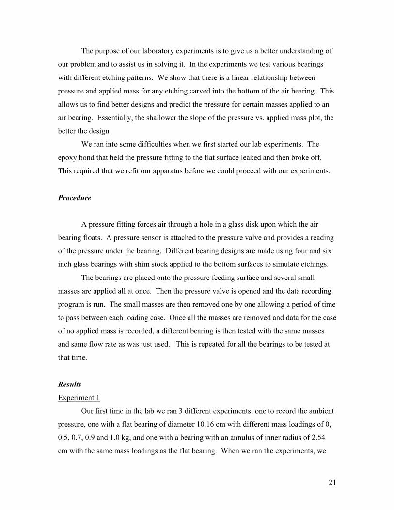
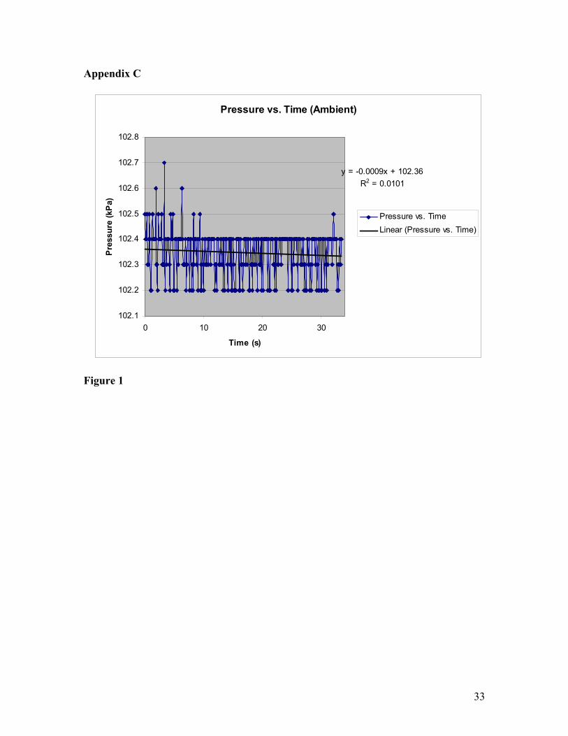
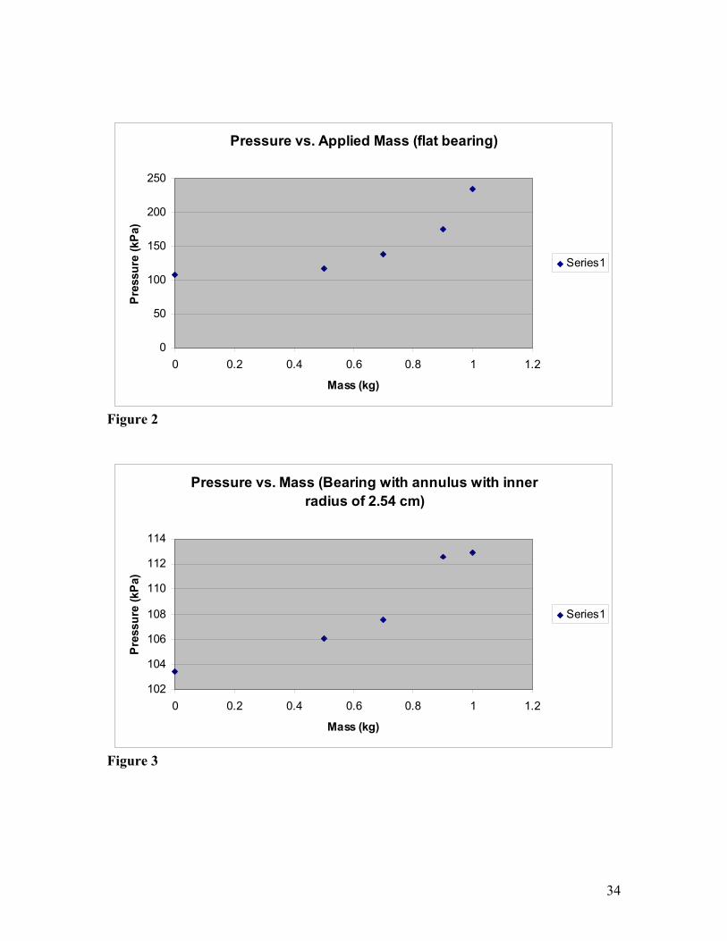
Our first time in the lab we ran 3 different experiments; one to record the ambient

pressure, one with a flat bearing of diameter 10.16 cm with different mass loadings of 0,

0.5, 0.7, 0.9 and 1.0 kg, and one with a bearing with an annulus of inner radius of 2.54

cm with the same mass loadings as the flat bearing. When we ran the experiments, we

21

tried to maintain the same gap height underneath the bearing during each experiment.

This was done by adjusting the pressure coming into the system. We recorded data for

each bearing in the form of pressure versus time. We then averaged the pressure for a

certain time with an applied mass and used that to construct a plot of pressure versus

mass. We hoped that this would show a linear relationship between pressure and mass.

However, the plots do not show a linear relationship very well, as can be seen in

Appendix C, Figures 2 and 3. This could be due to the fact that there were many sources

of error. For example, our instrument for measuring height allowed for very little

precision in our measurements. Furthermore, there could have been more leaks that we

missed.

Experiment 2

The second time in the lab we let the inlet pressure remain constant and the gap

height vary instead of adjusting the inlet pressure to keep the gap height constant. We

also used much lower applied masses on our bearings so that any unidentified leaks

would not be magnified.

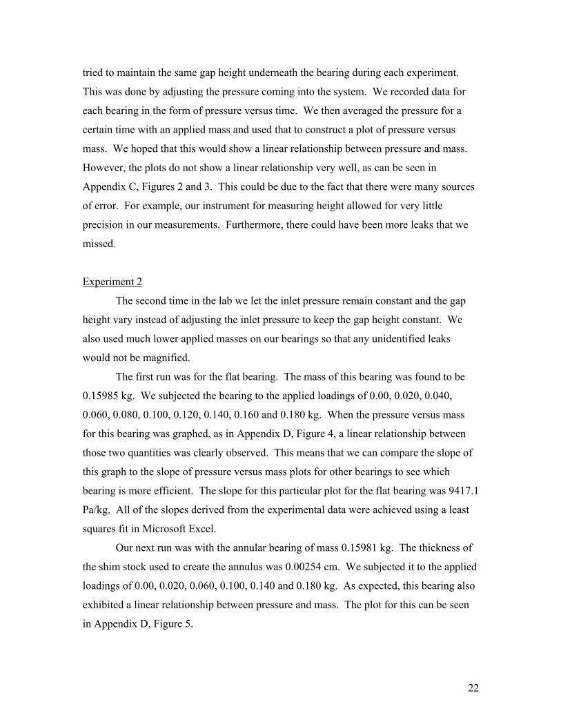
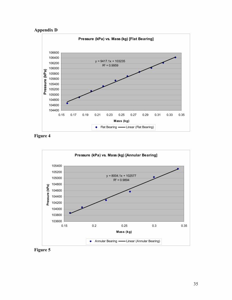
The first run was for the flat bearing. The mass of this bearing was found to be

0.15985 kg. We subjected the bearing to the applied loadings of 0.00, 0.020, 0.040,

0.060, 0.080, 0.100, 0.120, 0.140, 0.160 and 0.180 kg. When the pressure versus mass

for this bearing was graphed, as in Appendix D, Figure 4, a linear relationship between

those two quantities was clearly observed. This means that we can compare the slope of

this graph to the slope of pressure versus mass plots for other bearings to see which

bearing is more efficient. The slope for this particular plot for the flat bearing was 9417.1

Pa/kg. All of the slopes derived from the experimental data were achieved using a least

squares fit in Microsoft Excel.

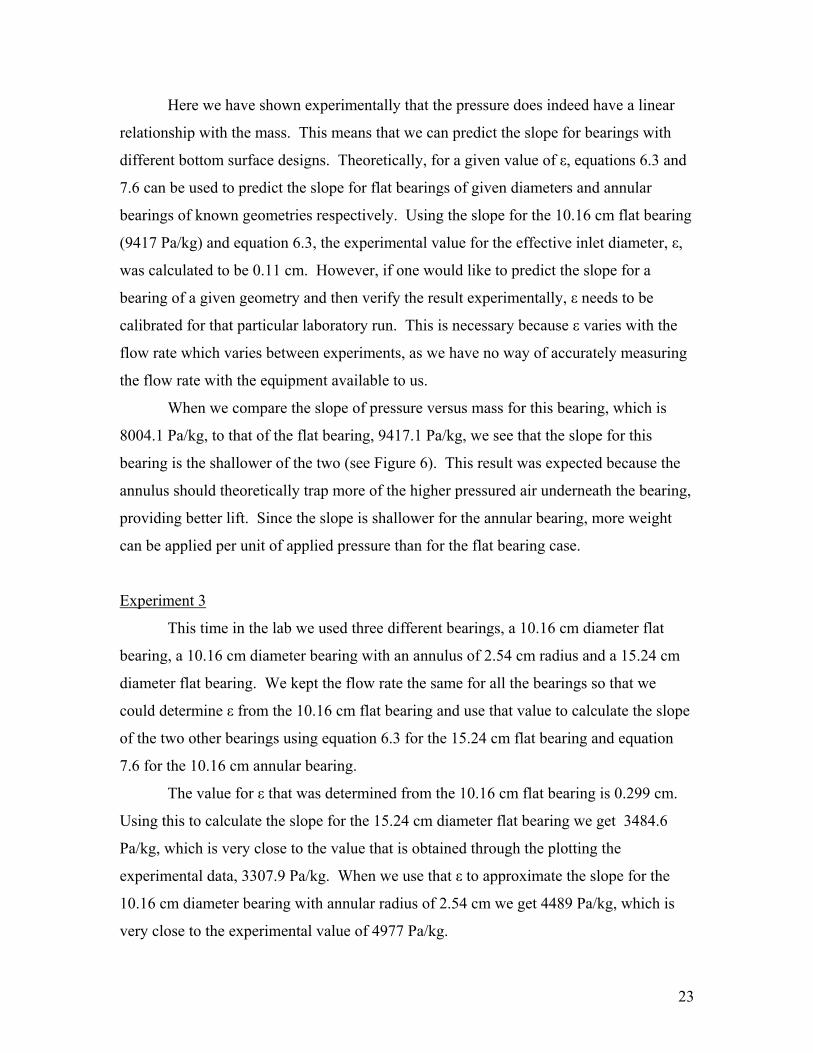
Our next run was with the annular bearing of mass 0.15981 kg. The thickness of

the shim stock used to create the annulus was 0.00254 cm. We subjected it to the applied

loadings of 0.00, 0.020, 0.060, 0.100, 0.140 and 0.180 kg. As expected, this bearing also

exhibited a linear relationship between pressure and mass. The plot for this can be seen

in Appendix D, Figure 5.

22

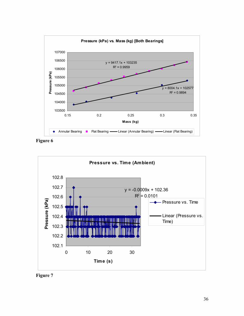
Here we have shown experimentally that the pressure does indeed have a linear

relationship with the mass. This means that we can predict the slope for bearings with

different bottom surface designs. Theoretically, for a given value of ε, equations 6.3 and

7.6 can be used to predict the slope for flat bearings of given diameters and annular

bearings of known geometries respectively. Using the slope for the 10.16 cm flat bearing

(9417 Pa/kg) and equation 6.3, the experimental value for the effective inlet diameter, ε,

was calculated to be 0.11 cm. However, if one would like to predict the slope for a

bearing of a given geometry and then verify the result experimentally, ε needs to be

calibrated for that particular laboratory run. This is necessary because ε varies with the

flow rate which varies between experiments, as we have no way of accurately measuring

the flow rate with the equipment available to us.

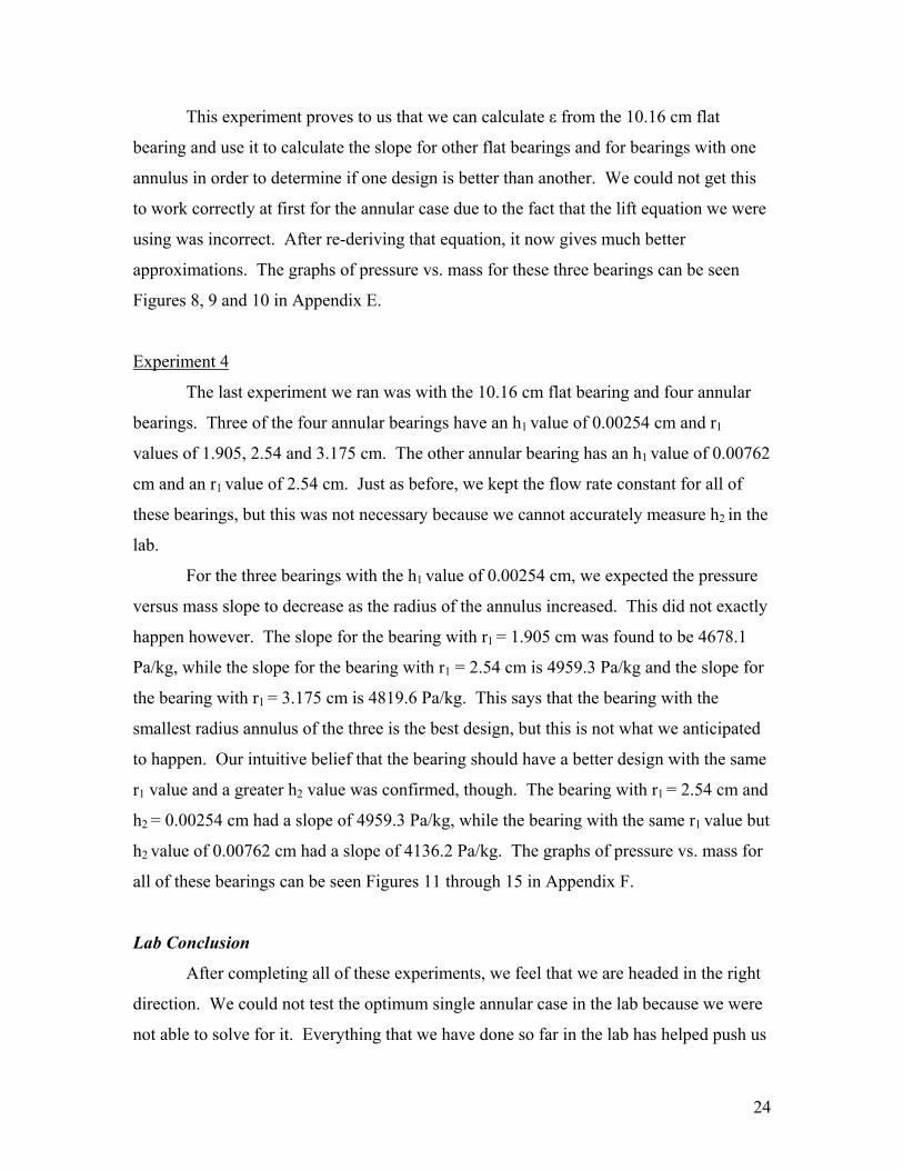
When we compare the slope of pressure versus mass for this bearing, which is

8004.1 Pa/kg, to that of the flat bearing, 9417.1 Pa/kg, we see that the slope for this

bearing is the shallower of the two (see Figure 6). This result was expected because the

annulus should theoretically trap more of the higher pressured air underneath the bearing,

providing better lift. Since the slope is shallower for the annular bearing, more weight

can be applied per unit of applied pressure than for the flat bearing case.

Experiment 3

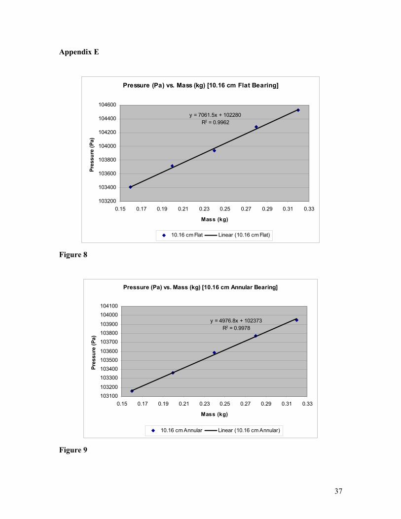
This time in the lab we used three different bearings, a 10.16 cm diameter flat

bearing, a 10.16 cm diameter bearing with an annulus of 2.54 cm radius and a 15.24 cm

diameter flat bearing. We kept the flow rate the same for all the bearings so that we

could determine ε from the 10.16 cm flat bearing and use that value to calculate the slope

of the two other bearings using equation 6.3 for the 15.24 cm flat bearing and equation

7.6 for the 10.16 cm annular bearing.

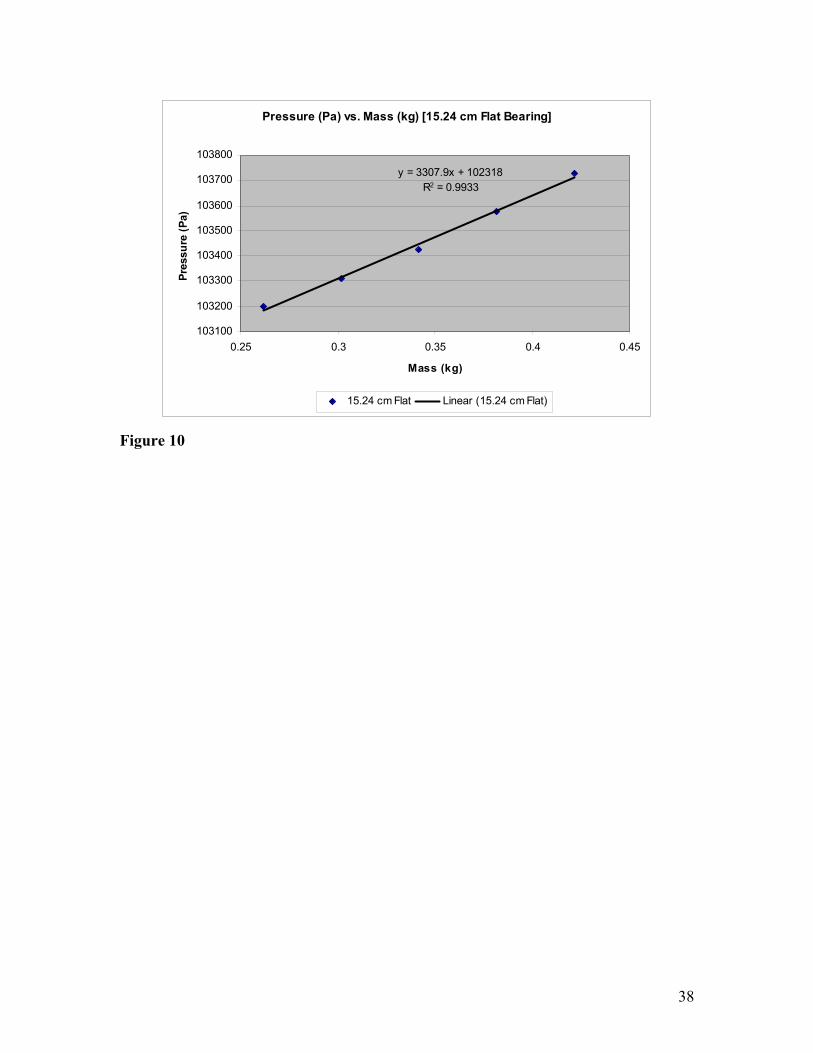
The value for ε that was determined from the 10.16 cm flat bearing is 0.299 cm.

Using this to calculate the slope for the 15.24 cm diameter flat bearing we get 3484.6

Pa/kg, which is very close to the value that is obtained through the plotting the

experimental data, 3307.9 Pa/kg. When we use that ε to approximate the slope for the

10.16 cm diameter bearing with annular radius of 2.54 cm we get 4489 Pa/kg, which is

very close to the experimental value of 4977 Pa/kg.

23

This experiment proves to us that we can calculate ε from the 10.16 cm flat

bearing and use it to calculate the slope for other flat bearings and for bearings with one

annulus in order to determine if one design is better than another. We could not get this

to work correctly at first for the annular case due to the fact that the lift equation we were

using was incorrect. After re-deriving that equation, it now gives much better

approximations. The graphs of pressure vs. mass for these three bearings can be seen

Figures 8, 9 and 10 in Appendix E.

Experiment 4

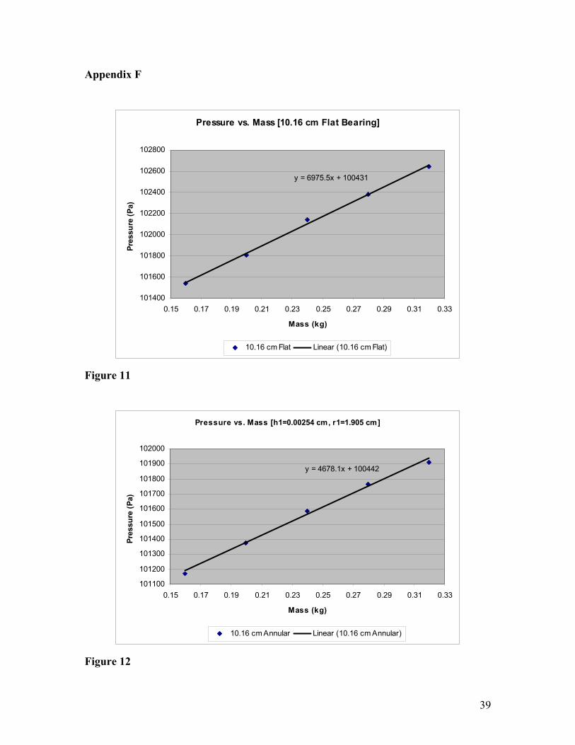
The last experiment we ran was with the 10.16 cm flat bearing and four annular

bearings. Three of the four annular bearings have an h1 value of 0.00254 cm and r1

values of 1.905, 2.54 and 3.175 cm. The other annular bearing has an h1 value of 0.00762

cm and an r1 value of 2.54 cm. Just as before, we kept the flow rate constant for all of

these bearings, but this was not necessary because we cannot accurately measure h2 in the

lab.

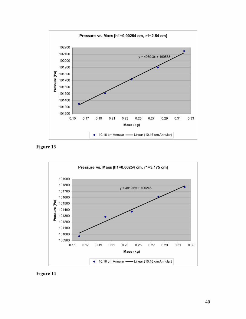
For the three bearings with the h1 value of 0.00254 cm, we expected the pressure

versus mass slope to decrease as the radius of the annulus increased. This did not exactly

happen however. The slope for the bearing with r1 = 1.905 cm was found to be 4678.1

Pa/kg, while the slope for the bearing with r1 = 2.54 cm is 4959.3 Pa/kg and the slope for

the bearing with r1 = 3.175 cm is 4819.6 Pa/kg. This says that the bearing with the

smallest radius annulus of the three is the best design, but this is not what we anticipated

to happen. Our intuitive belief that the bearing should have a better design with the same

r1 value and a greater h2 value was confirmed, though. The bearing with r1 = 2.54 cm and

h2 = 0.00254 cm had a slope of 4959.3 Pa/kg, while the bearing with the same r1 value but

h2 value of 0.00762 cm had a slope of 4136.2 Pa/kg. The graphs of pressure vs. mass for

all of these bearings can be seen Figures 11 through 15 in Appendix F.

Lab Conclusion

After completing all of these experiments, we feel that we are headed in the right

direction. We could not test the optimum single annular case in the lab because we were

not able to solve for it. Everything that we have done so far in the lab has helped push us

24

towards finding a solution for that case, but due to time constraints we did not get to that

point.

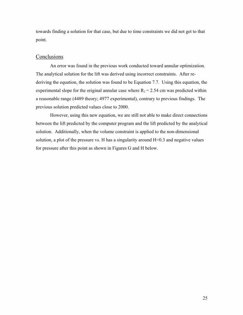
Conclusions An error was found in the previous work conducted toward annular optimization.

The analytical solution for the lift was derived using incorrect constraints. After re-

deriving the equation, the solution was found to be Equation 7.7. Using this equation, the

experimental slope for the original annular case where R1 = 2.54 cm was predicted within

a reasonable range (4489 theory; 4977 experimental), contrary to previous findings. The

previous solution predicted values close to 2000.

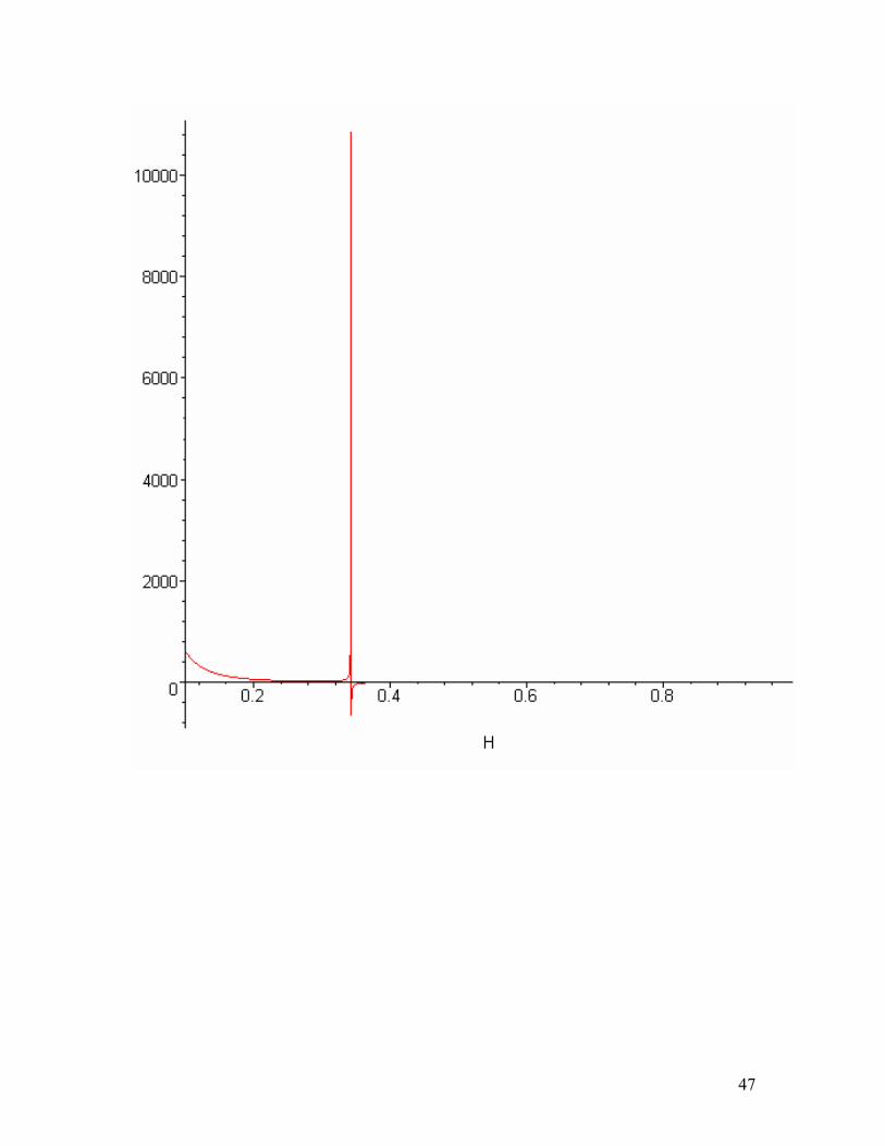
However, using this new equation, we are still not able to make direct connections

between the lift predicted by the computer program and the lift predicted by the analytical

solution. Additionally, when the volume constraint is applied to the non-dimensional

solution, a plot of the pressure vs. H has a singularity around H=0.3 and negative values

for pressure after this point as shown in Figures G and H below.

25

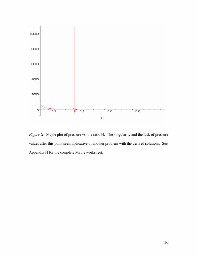
Figure G. Maple plot of pressure vs. the ratio H. The singularity and the lack of pressure

values after this point seem indicative of another problem with the derived solutions. See

Appendix H for the complete Maple worksheet.

26

Figure H. Maple plot of pressure for H=0.4 to 0.99. Note the negative values indicated

for pressure.

To move forward with this problem, the validity of the assumptions made should

be reconsidered. Additionally, the volume constraint should be critically analyzed.

27

Appendix A

Annotated Bibliography

1) Cameron. Basic Lubrication Theory, 2nd Edition. Ellis Horwood Limited,

England, 1976.

This book outlines basic mechanisms of lubrication. Reynolds equation is

derived and discussed in detail, which is of particular value for our

purposes. Oil is the primary mode of lubrication discussed in the book in

conjunction with several different types of bearings. Pressure equations

are discussed for most of the bearings that the book focuses on. These

equations may be good references as we develop our model further.

2) Szeri, Andras Z. Fluid Film Lubrication Theory & Design. Cambridge

University Press, New York, 1998.

This book primarily discusses various bearings and methods of

lubrication. The text does a good job of discussing the material from a

fluid mechanics standpoint. The Reynolds Equation is discussed, along

with Navier-Stokes Equations and the Equation of Continuity. Points of

interest in the text include some optimization discussion and flow stability.

The book also covers non-Newtonian fluids as well as gas lubrication,

either of which topics may be useful as model development and

refinement continues.

3) Grassam, N.S., Ed. and Powell, J.W., Ed. Gas Lubricated Bearings.

Butterworths, London, 1964.

Points of interest included in this reference are the design of aerodynamic

bearings, the design of externally pressurized bearings, and dynamic

characteristics of externally pressurized bearings. This book will be of

more use to the team as we refine the problem. The compressibility of gas

is taken into account for most of the applications of this book. At the

beginning stages of the model development we are assuming gas to be

28

incompressible. If we choose to alter this assumption at some point, this

reference may be of use.

4) Pinkus, Oscar and Sternlight, Beno. Theory of Hydrodynamic Lubrication.

McGraw-Hill Book Company, Inc., 1961.

Highlights in this book include basic differential equations, motion for

compressible and incompressible fluids, gas bearings, hydrodynamic

instability, non-Newtonian fluids, and experimental evidence. This

reference is heavy on mathematical theory and derivation, which will be of

use for the model development. Techniques for numerical analysis of

Reynolds equation are outlined which will prove very useful for the

project.

5) Chan, W.K. and Sun, Yuhong. “Analytical Modeling of Ultra-thin-film Bearings.”

Journal of Micromechanics and Microengineering 2003;13;463-473.

This journal article proposes an improved analytical model for ultra-thin-

film bearings based on the kinetic theory of gases. The model used in this

document, however, takes slip into account, whereas we are assuming no

slip in our model. The useful information from this article is the modified

Reynolds equations that are used and the fact that they look at flow rate

versus the inverse Knudsen number for a wide range of Knudsen numbers.

The Knudsen number is defined as the ratio of the mean free path to the

characteristic height. The flow rate at such a small gas thin-film thickness

has a very different behavior than that of macroscopic gas flow. This

digression is measured by the Knudsen number. We will have to take this

into account as our research and model development continues.

6) Galdi, Giovanni, Ed., Heywood, John, Ed., and Rannacher, Rolf, Ed.

Fundamental Directions in Mathematical Fluid Mechanics. Birkhauser Verlag,

Basel, 2000.

This book includes sections on Navier-Stokes initial-boundary value

problems, spectral approximations of Navier-Stokes equations, and finite

element methods for the incompressible Navier-Stokes equations. As the

Navier-Stokes equations are the equations of motion for an

29

incompressible, Newtonian fluid, the solver techniques this text provides

have great potential for use in this project. In particular, the section on

spectral methods may come of use when trying to solve for the finite

pressure distribution over a circular region as the optimization deals with.

7) Griebel, Micheal, Dornseifer, Thomas, and Neuhoeffer, Tilman. Numerical

Simulation in Fluid Dynamics: A Practical Introduction. SIAM, Philadelphia,

1998.

Useful aspects of this book are mathematical descriptions of flows,

numerical treatment of Navier-Stokes equations, and some example

applications. Again, at this phase in the project, there is some emphasis on

learning numerical techniques that can be applied to fluid mechanics and

dynamics.

8) Edwards, Dilwyn and Hamson, Mike. Guide to Mathematical Modeling. CRC

Press, Inc., Boca Raton, 1990.

This resource is not directly related to the problem at hand but rather helps

with the methodology of solving problems in general. The book discusses

the use of differential equations in modeling and provides some helpful

examples.

9) Bulirsch, R., Ed., Miele, A., Ed., Stoer, J., Ed., and Well, K.H., Ed. Optimal

Control: Calculus of Variations, Optimal Control Theory and Numerical

Methods. Birhauser Verlag, Basel,1993.

This book will become useful as optimization is further sought. Topics

include, optimality conditions and algorithms, numerical methods, and

analysis and synthesis of nonlinear systems. Also, there is a section

reserved for applications to mechanical and aerospace systems. The

examples within this section are optimizations for real-life applications

which will be useful in trying to optimize the real-life problem of the air

bearing.

30

10) Trefethen, Lloyd N. Spectral Methods in MATLAB. Society for Industrial and

Applied Mathematics, 2000.

This book is useful as we work towards using numerical methods to solve

the governing equations of our problem. It focuses on spectral methods

which can be applied to irregular geometries such as the circular geometry

relevant in the air bearing problem. The book is also full of MATLAB

code which we can build on and modify for our applications.

31

Appendix B with(VectorCalculus); Warning, the assigned names <,> and <|> now have a global binding Warning, these protected names have been redefined and unprotected: *, +, ., Vector, diff, int, limit, series

&x * + . <,> <|> AddCoordinates ArcLength BasisFormat Binormal, , , , , , , , , ,[CrossProduct Curl Curvature Del DirectionalDiff Divergence DotProduct Flux, , , , , , ,GetCoordinateParameters GetCoordinates Gradient Hessian Jacobian Laplacian, , , , ,LineInt MapToBasis Nabla PathInt PrincipalNormal RadiusOfCurvature, , , , , ,ScalarPotential SetCoordinateParameters SetCoordinates SurfaceInt TNBFrame, , , ,Tangen

,,

,t TangentLine TangentPlane TangentVector Torsion Vector VectorField, , , , , ,

VectorPotential Wronskian diff evalVF int limit series, , , , , , ],

SetCoordinates('polar'[r,theta]); polar ,r θ

P:=Gradient(p(r,theta),'polar'[r,theta]);

:= P +

∂

∂r ( )p ,r θ

re ∂

∂θ

( )p ,r θ

r θe

F:=(h(r,theta))^3*P;

:= F + ( )h ,r θ 3

∂

∂r ( )p ,r θ

re

( )h ,r θ 3

∂

∂θ

( )p ,r θ

r θe

Divergence(F);

( )h ,r θ 3

∂

∂r ( )p ,r θ 3 r ( )h ,r θ 2

∂

∂r ( )p ,r θ

∂

∂r ( )h ,r θ r ( )h ,r θ 3

∂

∂2

r2 ( )p ,r θ + +

3 ( )h ,r θ 2

∂

∂θ

( )p ,r θ

∂

∂θ

( )h ,r θ

r

( )h ,r θ 3

∂

∂2

θ2 ( )p ,r θ

r + + r

/

simplify(%);

( )h ,r θ 2 ( )h ,r θ

∂

∂r ( )p ,r θ r 3 r2

∂

∂r ( )p ,r θ

∂

∂r ( )h ,r θ r2 ( )h ,r θ

∂

∂2

r2 ( )p ,r θ + +

3

∂

∂θ

( )p ,r θ

∂

∂θ

( )h ,r θ ( )h ,r θ

∂

∂2

θ2 ( )p ,r θ + +

r2

32

Appendix C

Pressure vs. Time (Ambient)

y = -0.0009x + 102.36R2 = 0.0101

102.1

102.2

102.3

102.4

102.5

102.6

102.7

102.8

0 10 20 30

Time (s)

Pres

sure

(kPa

)

Pressure vs. TimeLinear (Pressure vs. Time)

Figure 1

33

Pressure vs. Applied Mass (flat bearing)

0

50

100

150

200

250

0 0.2 0.4 0.6 0.8 1 1.2

Mass (kg)

Pre

ssur

e (k

Pa)

Series1

Figure 2

Pressure vs. Mass (Bearing with annulus with inner radius of 2.54 cm)

102

104

106

108

110

112

114

0 0.2 0.4 0.6 0.8 1 1.2

Mass (kg)

Pre

ssur

e (k

Pa)

Series1

Figure 3

34

Appendix D

Pressure (kPa) vs. Mass (kg) [Flat Bearing]

y = 9417.1x + 103235R2 = 0.9959

104400104600

104800105000

105200105400

105600105800

106000106200

106400106600

0.15 0.17 0.19 0.21 0.23 0.25 0.27 0.29 0.31 0.33 0.35

Mass (kg)

Pre

ssur

e (k

Pa)

Flat Bearing Linear (Flat Bearing)

Figure 4

Pressure (kPa) vs. Mass (kg) [Annular Bearing]

y = 8004.1x + 102577R2 = 0.9894

103600

103800

104000

104200

104400

104600

104800

105000

105200

105400

0.15 0.2 0.25 0.3 0.35

Mass (kg)

Pres

sure

(kPa

)

Annular Bearing Linear (Annular Bearing)

Figure 5

35

Pressure (kPa) vs. Mass (kg) [Both Bearings]

y = 8004.1x + 102577R2 = 0.9894

y = 9417.1x + 103235R2 = 0.9959

103500

104000

104500

105000

105500

106000

106500

107000

0.15 0.2 0.25 0.3 0.35

Mass (kg)

Pres

sure

(kPa

)

Annular Bearing Flat Bearing Linear (Annular Bearing) Linear (Flat Bearing)

Figure 6

Pressure vs. Time (Ambient)

y = -0.0009x + 102.36R2 = 0.0101

102.1

102.2

102.3

102.4

102.5

102.6

102.7

102.8

0 10 20 30

Time (s)

Pres

sure

(kPa

)

Pressure vs. Time

Linear (Pressure vs.Time)

Figure 7

36

Appendix E

Pressure (Pa) vs. Mass (kg) [10.16 cm Flat Bearing]

y = 7061.5x + 102280R2 = 0.9962

103200

103400

103600

103800

104000

104200

104400

104600

0.15 0.17 0.19 0.21 0.23 0.25 0.27 0.29 0.31 0.33

Mass (kg)

Pres

sure

(Pa)

10.16 cm Flat Linear (10.16 cm Flat)

Figure 8

Pressure (Pa) vs. Mass (kg) [10.16 cm Annular Bearing]

y = 4976.8x + 102373R2 = 0.9978

103100103200

103300103400103500103600

103700103800103900

104000104100

0.15 0.17 0.19 0.21 0.23 0.25 0.27 0.29 0.31 0.33

Mass (kg)

Pres

sure

(Pa)

10.16 cm Annular Linear (10.16 cm Annular)

Figure 9

37

Pressure (Pa) vs. Mass (kg) [15.24 cm Flat Bearing]

y = 3307.9x + 102318R2 = 0.9933

103100

103200

103300

103400

103500

103600

103700

103800

0.25 0.3 0.35 0.4 0.45

Mass (kg)

Pres

sure

(Pa)

15.24 cm Flat Linear (15.24 cm Flat)

Figure 10

38

Appendix F

Pressure vs. Mass [10.16 cm Flat Bearing]

y = 6975.5x + 100431

101400

101600

101800

102000

102200

102400

102600

102800

0.15 0.17 0.19 0.21 0.23 0.25 0.27 0.29 0.31 0.33

Mass (kg)

Pres

sure

(Pa)

10.16 cm Flat Linear (10.16 cm Flat)

Figure 11

Pressure vs. Mass [h1=0.00254 cm, r1=1.905 cm]

y = 4678.1x + 100442

101100

101200

101300

101400

101500

101600

101700

101800

101900

102000

0.15 0.17 0.19 0.21 0.23 0.25 0.27 0.29 0.31 0.33

Mass (kg)

Pres

sure

(Pa)

10.16 cm Annular Linear (10.16 cm Annular)

Figure 12

39

Pressure vs. Mass [h1=0.00254 cm, r1=2.54 cm]

y = 4959.3x + 100538

101200

101300

101400

101500

101600

101700

101800

101900

102000

102100

102200

0.15 0.17 0.19 0.21 0.23 0.25 0.27 0.29 0.31 0.33

Mass (kg)

Pres

sure

(Pa)

10.16 cm Annular Linear (10.16 cm Annular)

Figure 13

Pressure vs. Mass [h1=0.00254 cm, r1=3.175 cm]

y = 4819.6x + 100245

100900

101000

101100

101200

101300

101400

101500

101600

101700

101800

101900

0.15 0.17 0.19 0.21 0.23 0.25 0.27 0.29 0.31 0.33

Mass (kg)

Pres

sure

(Pa)

10.16 cm Annular Linear (10.16 cm Annular)

Figure 14

40

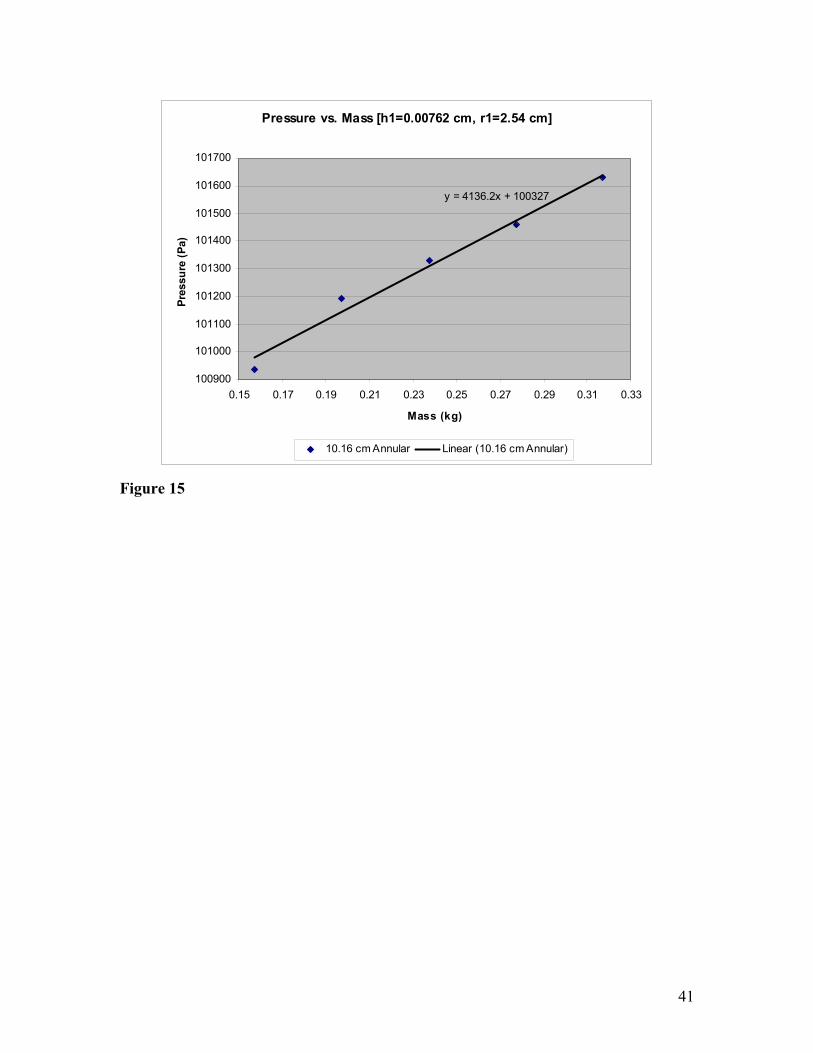
Pressure vs. Mass [h1=0.00762 cm, r1=2.54 cm]

y = 4136.2x + 100327

100900

101000

101100

101200

101300

101400

101500

101600

101700

0.15 0.17 0.19 0.21 0.23 0.25 0.27 0.29 0.31 0.33

Mass (kg)

Pres

sure

(Pa)

10.16 cm Annular Linear (10.16 cm Annular)

Figure 15

41

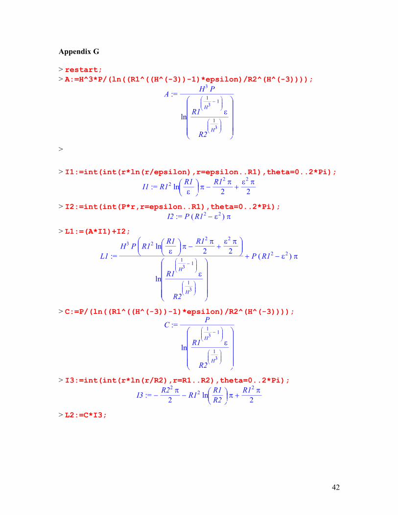
Appendix G > restart; > A:=H^3*P/(ln((R1^((H^(-3))-1)*epsilon)/R2^(H^(-3))));

:= A H3 P

ln R1

− 1

H31

ε

R2

1

H3

>

> I1:=int(int(r*ln(r/epsilon),r=epsilon..R1),theta=0..2*Pi);

:= I1 − + R12

ln

R1ε

πR12 π

2ε2 π

2

> I2:=int(int(P*r,r=epsilon..R1),theta=0..2*Pi); := I2 P ( ) − R12 ε2 π

> L1:=(A*I1)+I2;

:= L1 + H3 P

− + R12

ln R1

επ

R12 π2

ε2 π2

lnR1

− 1

H31

ε

R2

1

H3

P ( ) − R12 ε2 π

> C:=P/(ln((R1^((H^(-3))-1)*epsilon)/R2^(H^(-3))));

:= C P

ln R1

− 1

H3 1

ε

R2

1

H3

> I3:=int(int(r*ln(r/R2),r=R1..R2),theta=0..2*Pi);

:= I3 − − + R22 π

2 R12

ln

R1R2 π

R12 π2

> L2:=C*I3;

42

:= L2P

− − +

R22 π2 R12

ln R1

R2 πR12 π

2

ln R1

− 1

H3 1

ε

R2

1

H3

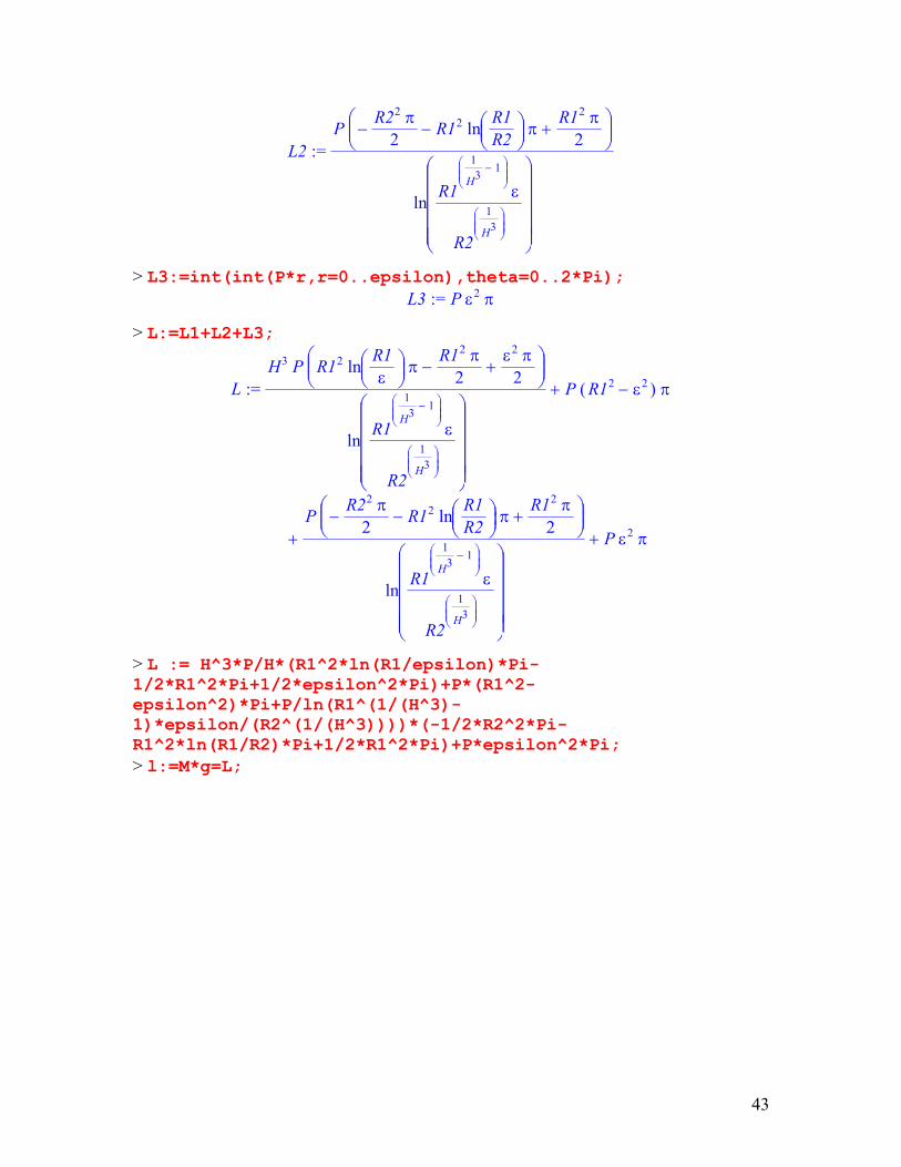
> L3:=int(int(P*r,r=0..epsilon),theta=0..2*Pi); := L3 P ε2 π

> L:=L1+L2+L3;

LH3 P

− + R12

ln R1

επ

R12 π2

ε2 π2

ln R1

− 1

H3 1

ε

R2

1

H3

P ( ) − R12 ε2 π + :=

P

− − +

R22 π2 R12

ln R1

R2 πR12 π

2

lnR1

− 1

H31

ε

R2

1

H3

P ε2 π + +

> L := H^3*P/H*(R1^2*ln(R1/epsilon)*Pi-1/2*R1^2*Pi+1/2*epsilon^2*Pi)+P*(R1^2-epsilon^2)*Pi+P/ln(R1^(1/(H^3)-1)*epsilon/(R2^(1/(H^3))))*(-1/2*R2^2*Pi-R1^2*ln(R1/R2)*Pi+1/2*R1^2*Pi)+P*epsilon^2*Pi; > l:=M*g=L;

43

l M gH3 P

− + R12

ln R1

επ

R12 π2

ε2 π2

lnR1

− 1

H31

ε

R2

1

H3

P ( ) − R12 ε2 π + = :=

P

− − +

R22 π2 R12

ln R1

R2 πR12 π

2

lnR1

− 1

H31

ε

R2

1

H3

P ε2 π + +

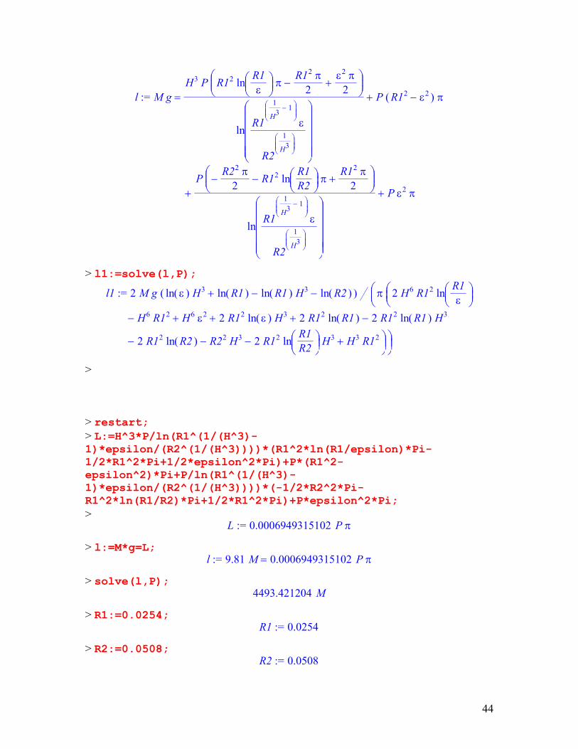
> l1:=solve(l,P);

l1 2 M g ( ) + − − ( )ln ε H3 ( )ln R1 ( )ln R1 H3 ( )ln R2 π 2 H6 R12

ln R1

ε

:=

H6 R12 H6 ε2 2 R12 ( )ln ε H3 2 R12 ( )ln R1 2 R12 ( )ln R1 H3 − + + + −

2 R12 ( )ln R2 R22 H3 2 R12

ln R1

R2 H3 H3 R12 − − − +

>

> restart; > L:=H^3*P/ln(R1^(1/(H^3)-1)*epsilon/(R2^(1/(H^3))))*(R1^2*ln(R1/epsilon)*Pi-1/2*R1^2*Pi+1/2*epsilon^2*Pi)+P*(R1^2-epsilon^2)*Pi+P/ln(R1^(1/(H^3)-1)*epsilon/(R2^(1/(H^3))))*(-1/2*R2^2*Pi-R1^2*ln(R1/R2)*Pi+1/2*R1^2*Pi)+P*epsilon^2*Pi; >

:= L 0.0006949315102 P π

> l:=M*g=L; := l = 9.81 M 0.0006949315102 P π

> solve(l,P); 4493.421204 M

> R1:=0.0254; := R1 0.0254

> R2:=0.0508; := R2 0.0508

44

> epsilon:=0.00287; := ε 0.00287

> H:=0.5; := H 0.5

> g:=9.81; := g 9.81

45

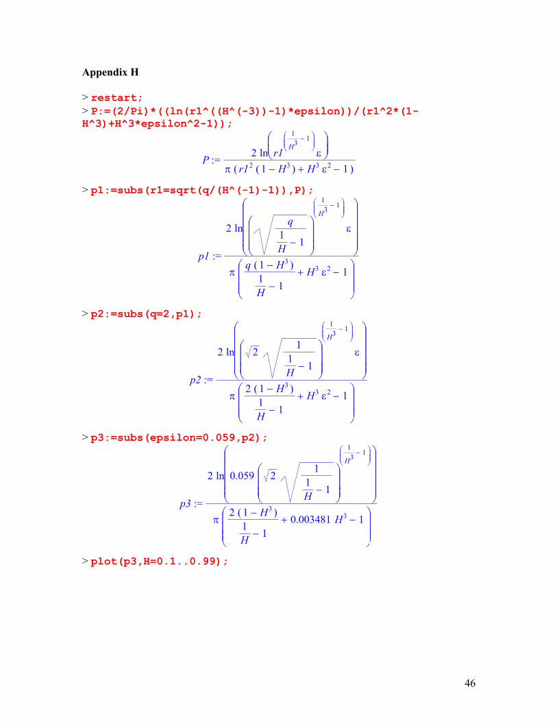
Appendix H > restart; > P:=(2/Pi)*((ln(r1^((H^(-3))-1)*epsilon))/(r1^2*(1-H^3)+H^3*epsilon^2-1));

:= P 2

ln r1

− 1

H31

επ ( ) + − r12 ( ) − 1 H3 H3 ε2 1

> p1:=subs(r1=sqrt(q/(H^(-1)-1)),P);

:= p1

2

ln

q

− 1H 1

− 1

H3 1

ε

π

+ − q ( ) − 1 H3

− 1H 1

H3 ε2 1

> p2:=subs(q=2,p1);

:= p2

2

ln

21

− 1H 1

− 1

H31

ε

π

+ − 2 ( ) − 1 H3

− 1H 1

H3 ε2 1

> p3:=subs(epsilon=0.059,p2);

:= p3

2

ln 0.059

21

− 1H 1

− 1

H31

π

+ − 2 ( ) − 1 H3

− 1H 1

0.003481 H3 1

> plot(p3,H=0.1..0.99);

46

47